Trace gas fluxes from tidal salt marsh soils: implications for carbon–sulfur biogeochemistry

Tidal salt marsh soils can be a dynamic source of greenhouse gases such as carbon dioxide (CO₂), methane (CH₄), and nitrous oxide (N₂O), as well as sulfur-based trace gases such as carbon disulfide (CS₂) and dimethylsulfide (DMS) which play roles in global climate and carbon–sulfur biogeochemistry. Due to the difficulty in measuring trace gases in coastal ecosystems (e.g., flooding, salinity), our current understanding is based on snapshot instantaneous measurements (e.g., performed during daytime low tide) which complicates our ability to assess the role of these ecosystems for natural climate solutions. We performed continuous, automated measurements of soil trace gas fluxes throughout the growing season to obtain high-temporal frequency data and to provide insights into magnitudes and temporal variability across rapidly changing conditions such as tidal cycles. We found that soil CO₂ fluxes did not show a consistent diel pattern, CH₄, N₂O, and CS₂ fluxes were highly variable with frequent pulse emissions (> 2500 %, > 10 000 %, and > 4500 % change, respectively), and DMS fluxes only occurred midday with changes > 185 000 %. When we compared continuous measurements with discrete temporal measurements (during daytime, at low tide), discrete measurements of soil CO₂ fluxes were comparable with those from continuous measurements but misrepresent the temporal variability and magnitudes of CH₄, N₂O, DMS, and CS₂. Discrepancies between the continuous and discrete measurement data result in differences for calculating the sustained global warming potential (SGWP), mainly by an overestimation of CH₄ fluxes when using discrete measurements. The high temporal variability of trace gas fluxes complicates the accurate calculation of budgets for use in blue carbon accounting and earth system models.

1 Introduction

Coastal vegetated ecosystems, such as tidal salt marshes, mangrove forests, and seagrass beds, provide a wide range of ecosystem services such as mitigating storm surge and providing nursery areas for fish species (Barbier et al., 2011; Möller et al., 2014). They also can potentially store large amounts of carbon at rates 40 times higher than tropical rainforests (Rosentreter et al., 2018; Duarte et al., 2005) and are referred to as “blue carbon” ecosystems. The importance of coastal vegetated ecosystems in climate change policies has been recognized by the Paris Agreement (UNFCCC, 2015). Prior to the Paris Agreement, there had been increasing interest in better quantifying the net balance between carbon storage and carbon release in coastal vegetated ecosystems for both scientific and carbon market purposes. For example, the Verified Carbon Standard developed a methodology to assess and verify the amount of carbon removed from the atmosphere in tidal wetland and seagrass restoration projects for carbon market purposes (Emmer et al., 2021). However, there are major knowledge gaps in assessing blue carbon in coastal vegetated ecosystems. Specifically, the high spatial and temporal variability of greenhouse gas (GHG) emissions, particularly for CH₄ and N₂O, in coastal vegetated ecosystems complicates blue carbon offset calculations (Rosentreter et al., 2021; Capooci et al., 2019; Al-Haj and Fulweiler, 2020; Murray et al., 2015). Thus, there is a need for developing measurement protocols to fully quantify the contribution of multiple GHGs in blue carbon ecosystems.

To improve our understanding of blue carbon ecosystems in global biogeochemical cycles we need to think beyond traditional GHG trace gases (i.e., CO₂, CH₄, N₂O). Tidal salt marshes produce sulfur-based trace gases due to the prevalence of sulfur cycling within their soils, which has implications for carbon–sulfur biogeochemistry and the global climate. While coastal areas are major sources of sulfur gases (Kellogg et al., 1972), there is large uncertainty in emission rates (Carroll et al., 1986; Andreae and Jaeschke, 1992; Brimblecombe, 2014). Dimethyl sulfide (DMS) is one of the dominant sulfur-based gases emitted from salt marshes (Hines, 1996) and is considered a climate cooling gas, in part due to its oxidation to SO₄ in the atmosphere (Thomas et al., 2010; Watts, 2000; Charlson et al., 1987). Dimethylsulfoniopropionate (DMSP), a DMS precursor, can be produced by salt marsh plant species Spartina alterniflora, S. anglica, and S. foliosa (Hines, 1996). DMS plays an important role in linking together carbon and sulfur biogeochemistry in salt marsh soils. It can be decomposed by not only sulfate-reducing bacteria, but can also act as a non-competitive substrate for methylotrophic methanogenesis (Kiene, 1988; Kiene and Visscher, 1987; Oremland et al., 1982) which allows methane production to occur in soils dominated by sulfate reduction (Seyfferth et al., 2020). Another sulfur-based trace gas released from tidal salt marshes is carbon disulfide (CS₂), which has an insignificant global warming potential and a short atmospheric lifetime (Brühl et al., 2012). However, CS₂ is a precursor to carbonyl sulfide (COS; Whelan et al., 2013). COS is the most abundant reduced sulfur compound in the atmosphere and can form sulfate aerosols that affect the earth's radiative properties by reflecting sunlight, thereby having a cooling effect on the climate (Watts, 2000; Taubman and Kasting, 1995). Despite sulfur-based trace gases playing a role in wetland soil biogeochemistry and in global climate, there is a need to quantify coastal wetland sulfur emissions and to connect those emissions to both the salt marsh sulfur cycle and to global budgets (DeLaune et al., 2002; Whelan et al., 2013).

Historically, both soil GHGs and S-based fluxes are measured using manual survey chambers, particularly during daytime low tide (e.g., De Mello et al., 1987) when soils are less likely to be submerged and are accessible to researchers. Measurements at high tide in salt marshes are difficult due to both reduced access to the marsh platform and reduced fluxes. Gases from the soil mix with the overlying water column and move more slowly through water compared with air, contributing to a decline in fluxes during high tide (Moffett et al., 2010). Manual measurements have a number of advantages, including the ability to sample over large areas over short periods of time (Moseman-Valtierra et al., 2016; Simpson et al., 2019), but these measurements are labor intensive and provide limited information regarding temporal variability (Koskinen et al., 2014; Savage et al., 2014; Vargas et al., 2011). On the other hand, recent advances in high temporal frequency soil efflux measurements (Capooci and Vargas, 2022a; Diefenderfer et al., 2018; Järveoja et al., 2018) have provided researchers with unprecedented temporal information to better understand diel and tidal patterns, as well as the influence of pulse events on trace gas emissions within salt marshes. While the use of automated systems is becoming more common in measuring salt marsh fluxes (Capooci and Vargas, 2022a; Diefenderfer et al., 2018; Trifunovic et al., 2020), their use is limited by high instrumentation costs, electricity requirements, and logistical challenges associated with installing these instruments in an environment prone to flooding and with high humidity. As automated systems become more prevalent, researchers are provided with the opportunity to evaluate data collected from manual measurements, such as daily means, that have been used to inform models and budgets, particularly for understudied trace gases such as N₂O, CS₂, and DMS.

The objective of this study is to characterize the spatial and temporal variability of trace gases from soils in a tidal salt marsh. Specifically, we focus on CO₂, CH₄, N₂O, CS₂, and DMS to assess the differences between measurements taken at a particular time of day (i.e., daytime low tide) and measurements with high temporal frequency (i.e., continuous hourly measurements for ∼ 72 h). Few studies have measured GHG fluxes from tidal salt marshes using continuous, automated measurements (Diefenderfer et al., 2018; Capooci and Vargas, 2022a), and this is a pioneering study that provides unprecedented information about the magnitudes and patterns of CS₂ and DMS fluxes via continuous measurements. Furthermore, this study tests whether traditional measurement protocols based on discrete temporal measurements provide similar information as data derived from continuous measurements, including the calculation of the sustained global warming potential (SGWP). Development of new technologies and incorporation of this information has important implications for calculating greenhouse and trace gas budgets, as well as the role salt marshes play in global biogeochemical cycles.

2 Materials and methods

2.1 Study site

The study was conducted at St Jones Reserve, the brackish estuarine component of the Delaware National Estuarine Research Reserve. The site is part of the Delaware Estuary and is tidally connected to the Delaware Bay via the St Jones River. St Jones is classified as a mesohaline tidal salt marsh (DNREC, 1999) and has silty clay loam soils (10 % sand, 61 % silt, 29 % loam; Capooci et al., 2019). The study was conducted in a section of the marsh dominated by Spartina alterniflora (= Sporobolus alterniflorus (Loisel.); Peterson et al., 2014) and will be referred to as “SS” as established in previous studies (Seyfferth et al., 2020; Capooci and Vargas, 2022a). This area is lower in elevation relative to the rest of the marsh, is characterized by sulfur reduction (Seyfferth et al., 2020), and covers ∼ 66 % of the salt marsh landscape (Vázquez-Lule and Vargas, 2021). The SS site rarely floods during high tide due to its distance from the tidal creek (∼ 50 m), as well as the presence of a berm located adjacent to the tidal creek (Seyfferth et., 2020; Hill et al., 2021).

2.2 Experimental setup

The experiment was performed over the course of six campaigns to cover a full growing season: greenup (G), maturity (M), senescence (S), and dormancy (D) as described by the canopy phenology of the study site (Hill et al., 2021). The campaigns began during the latter half of the 2020 growing season and continued into the beginning of the 2021 growing season (M1: 29 June to 2 July; M2: 31 July to 3 August; S1: 31 August to 3 September; S2: 28 September to 1 October; D1: 13 to 16 April; and G1: 31 May to 3 June) due to delays related to the COVID-19 pandemic. We installed six PVC collars (diameter: 20 cm), placed ∼ 1.2 m apart, 4 months prior to the beginning of the experiment in 2020. Collars were placed in a S. alterniflora area of the marsh near the boardwalk to minimize impacts to the marsh, as well as to easily access boardwalk power outlets. Any vegetation that grew inside these collars in between campaigns was carefully clipped at the base of the stem prior to each campaign. Vegetation was clipped on a frequent basis to minimize stem diameters and thereby reduced the effects of plant-mediated gas transport. These collars were used to set down six opaque automated chambers (LICOR 8100-104, Lincoln, NE, USA; volume: 4071.1 cm³) to measure trace gas fluxes as described below.

2.3 Trace gas flux measurements and QA/QC

The autochambers were coupled with a closed-path infrared gas analyzer (LI-8100A, LICOR, Lincoln, NE, USA) and a Fourier transform infrared spectrometer (DX4040, Gasmet Technologies Oy, Vantaa, Finland). The LI-8100A and the DX4040 were connected in parallel since the DX4040 has its own internal pump and flow rates. Trace gas fluxes were measured once per hour per chamber (i.e., all six chambers were measured within an hour). Measurements were 5 min long and each chamber was flushed for 5 min total (pre-purge and post-purge were both 2.5 min long) to help reduce the impacts of humidity on the instruments. Each campaign lasted approximately 72 h where approximately 416 measurements were recorded. Campaigns were short in length due to electrical power limitations and to minimize instrumentation damage due to the corrosive environmental conditions.

At the beginning of each campaign and every 24 h after, we performed a zero calibration on the DX4040 using ultra-pure 99.999 % N₂ gas. It is recommended that zero calibrations be performed every 24 h and when the ambient temperature changes by 10 ^∘C, so the experiment was paused for ∼ 30 min during the zero calibrations each day. Gas fluxes were calculated using Soil Flux Pro (v4.2.1, LICOR, Lincoln, NE, USA) and underwent standardized quality assurance and quality control (QA/QC) protocols as established in previous publications (Capooci et al., 2019; Petrakis et al., 2017). The QA/QC included several steps. First, all values due to instrumental errors, such as an insufficient chamber closure seal, were removed. These errors were identified by the SoilFluxPro software. Second, the R² for the linear and exponential fits of trace gas emissions were compared and the fit with the higher R² was chosen. Third, all fluxes that occurred when the R² of CO₂ was < 0.90 were removed. Low R² values indicate that the soil micrometeorological conditions were not stable during the measurement. Finally, all negative CO₂ fluxes were removed since they were likely erroneous.

2.4 Ancillary measurements

Meteorological (station: delsjmet-p) and water quality (station: Aspen Landing) data were obtained from the National Estuarine Research Reserve's Centralized Data Management Office (CDMO) and collected according to their protocol (System-wide Monitoring Program). Meteorological data were collected using a CR1000 Meteorological Monitoring Station (Campbell Scientific, Logan, UT, USA). Water quality data were measured using a YSI 6600 sonde (YSI Inc., OH, USA). Both datasets were cleaned and gap filled following the protocol established in Capooci et al. (2022a).

Phenological data were obtained from the PhenoCam network (site: stjones, Seyednasrollah et al., 2019) as described previously (Trifunovic et al., 2020; Hill et al., 2021). Briefly, a single midday photo (12:00:00 h) was selected for each of the days in the study period and was visually inspected to remove images with obvious distortions. Since the images included a variety of vegetation types, the region of interest delineated to only the area containing S. alterniflora, the main species at the study site. Then the phenopix R package (Filippa et al., 2020) was used to extract and calculate the greenness index, as well as delineate the phenophases for the study period (Hill et al., 2021).

2.5 Data analyses

Daily averages and associated standard deviations were calculated for meteorological and water quality data, except for the greenness index. Soil trace flux data were averaged into hourly and daily means and standard deviations. For heat maps, average hourly and campaign-length coefficients of variation were calculated.

We extracted measurements from the time series of the automated measurements to represent information collected from discrete temporal measurements conducted during daytime low tide. This approach aimed to represent a measurement protocol derived from manual (i.e., survey) measurements where most measurements are performed at daytime and low tide for logistical reasons. To identify and extract these measurements, we identified when low tide occurred during each day (between 09:00:00 and 17:00:00 h) of the campaigns from water level data obtained from the tidal creek. All automated measurements that fell between 1 h before and 1 h after low tide were extracted, averaged into a daily value, and classified as “discrete” measurements. For example, if low tide fell at 13:00:00 h, all continuous measurements that fell between 12:00:00 and 14:00:00 h were then extracted and averaged to obtain a daily mean. Daily means were also calculated for all automated measurements collected during the day and will be referred to as the “continuous” daily mean. Differences in the means and distributions of the continuous and discrete fluxes were assessed using a t test and a Kolmogorov–Smirnov test, respectively.

Sustained global warming potential was calculated for both the campaign-long and daytime low tide fluxes for CO₂, CH₄, and N₂O. The SGWP accounts for sustained gas emissions over time compared with the global warming potential which accounts for a pulse emission over time (Neubauer and Megonigal, 2019). To calculate the SGWP, data from days 2 and 3 of each campaign were used since measurements on days 1 and 4 did not always occur during daytime low tide. Fluxes were converted into g m⁻² and multiplied by the 20- and 100-year SGWP (Neubauer and Megonigal, 2019). The SGWP values were compared to see whether extrapolating SGWP from daily-averaged manual measurements done at low tide yielded values similar to those of hourly-averaged from high temporal frequency measurements.

3 Results

3.1 Meteorological and water quality

Air temperature and greenness index show traditional seasonal patterns of temperate salt marshes (Fig. 1). Daily mean air temperature ranged from −3.5 to 29.9^∘C, with an average daily temperature of 13.8 ± 9.1^∘C, while greenness index ranged from 0.30 to 0.42 with an average of 0.34 ± 0.04. Relative humidity, barometric pressure, water level, and salinity varied throughout the year. Relative humidity ranged from 32.6 % to 100 % with an average of 79.1 % ± 16.7 %. Barometric pressure was between 999.7 and 1036 mb with an average value of 1018.3 ± 6.8 mb. Daily water level ranged from −0.30 to 0.76 m with an average height of 0.25 ± 0.2 m, while salinity ranged from 1.1 to 20.4 ppt with an average of 8.0 ± 4.45 ppt.

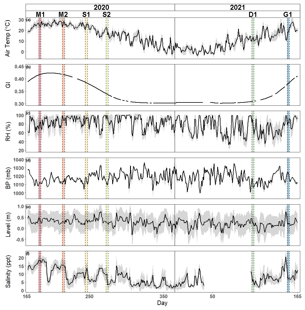
Figure 1 Time series of hourly mean ± SD gray shaded region of (a) air temperature, (b) greenness index, (c) relative humidity, (d) barometric pressure, (e) water level, and (f) salinity from 14 June 2020 to 14 June 2021. Vertical shaded areas correspond to each of the campaigns (M: maturity; S: senescence; D: dormancy; G: greenup).

3.2 Greenhouse gas and sulfur-based trace gas patterns and variability

Average CO₂ fluxes were significantly different in each campaign, with the highest average fluxes occurring during the G1 campaign and the lowest during the D1 campaign (Fig. 2a). During some campaigns, such as S1, CO₂ fluxes did not show similar temporal patterns between chambers, whereas during other campaigns, such as M2 and G1, all six chambers had similar patterns. While there is a seasonal pattern in CO₂ fluxes, with higher fluxes occurring during warmer months, diel patterns were not consistent between campaigns. One notable exception is the G1 campaign, during which a clear diel pattern was observed. CO₂ fluxes had consistent variability from one hour to the next during each of the six campaigns (Fig. 3a), with overall average variability ranging from 28.9 % during M2 to 49.6 % during Dl.

CH₄ fluxes were low most of the time, particularly during the G1 campaign (Fig. 2b). However, CH₄ pulses occurred during five out of the six campaigns, with S1 and S2 having the most frequent pulse emissions. S2 had the largest CH₄ pulse, 13 488 nmol m⁻² s⁻¹, which was 2599 % higher than the average flux. The highest average CH₄ fluxes also occurred during S1 and S2, while the highest hourly variability occurred in both S1 and S2, as well as in M2 (Fig. 3b). Mean CH₄ variability ranged from −108 % in M1 to 91.0 % in S1.

Most N₂O fluxes were near zero, with periodic pulses of emissions or uptake that ranged from −33.8 to 19.0 nmol m⁻² s⁻¹ (Fig. 2c), with a maximum percent change from the mean of 10 231 %. Of the six campaigns, four (M1, S2, D1, and G1) had net N₂O uptake, while two campaigns (M2, S1) had net N₂O fluxes. There were no significant differences between campaigns except for M1 and S1. Meanwhile, N₂O fluxes had very high hourly variability ranging from −106 964 % to 26 208 % (Fig. 3c). Consequently, average variability during each campaign was highly variable from −1032 % to 129 %.

Similarly to CH₄ and N₂O, CS₂ fluxes were low the majority of the time, with occasional pulses of emissions or uptake (Fig. 2d). CS₂ fluxes ranged from −386.9 to 306.2 nmol m⁻² s⁻¹, with a maximum percent change from the mean of 4785 %. All campaigns had net emissions despite periodic pulses of CS₂ uptake. CS₂ fluxes also had high hourly variability, with overall means for each campaign ranging from −70.2 % during D1 to 2254 % during M2 (Fig. 3d).

DMS emissions were zero for most of the campaigns (Fig. 2e). Pulses of emissions and uptake tended to occur during midday. DMS fluxes ranged from −158.5 to 230 nmol m⁻² s⁻¹, with a maximum percent change from the mean of 185 987 %. D1 and G1 had net uptake, while the other four campaigns had net emissions of DMS. During periods of emissions and uptake, hourly variability ranged from −870.5 % to 888.7 % (Fig. 2e). The extended periods of no DMS fluxes contributed to low overall mean variability during each campaign, ranging from −2.45 % in S2 to 35.7 % in M2.

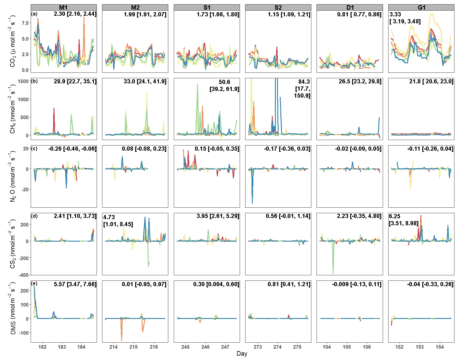
Figure 2 Time series of fluxes from each chamber during each campaign for (a) CO₂, (b) CH₄, (c) N₂O, (d) CS₂, and (e) DMS. Each color designates a different chamber. The campaign means [LCI = lower 95 % confidence interval, UCI = upper 95 % confidence interval] are listed on each panel. The y axis for CH₄ fluxes was shortened to show the variability. The full range of CH₄ fluxes during S2 can be seen in Fig. S1 in the Supplement.

Figure 3 Heat maps of hourly coefficient of variance (CV) for (a) CO₂, (b) CH₄, (c) N₂O, (d) CS₂, and (e) DMS during each campaign. Each pixel represents the average CV for that hour. The mean CV for each campaign is listed in the μ column. Grayed-out pixels represent NA. Note that the legend scale is different for each gas and campaigns start at 15:00:00 h on day 1 and end at 13:00:00 h on day 4.

3.3 Comparisons between continuous and discrete measurement scenarios

A subset of the continuous measurements that fall during daytime low tide was selected to represent data collected using traditional discrete, manual measurements which are commonly reported for tidal salt marshes. Information from continuous and discrete datasets are compared to elevate whether they provide similar distributions, daily means, flux–temperature relationships, and SGWP.

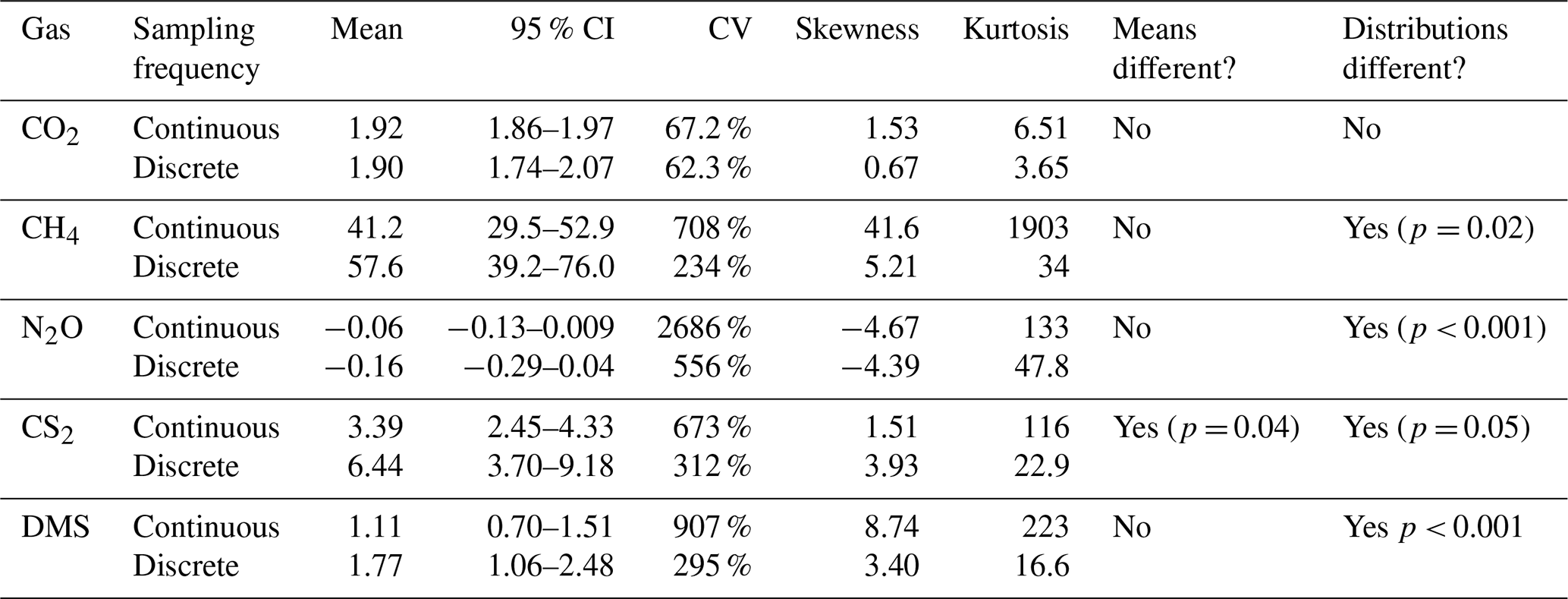
Continuous and discrete flux distributions can be seen via density plots (Fig. 4). While the distributions for continuous and discrete fluxes overlap for each of the five gases, four of the five gases have significantly different distributions of fluxes when comparing the continuous and the discrete datasets (Table 1). The only gas that had similar distributions between the two sampling intervals was CO₂ (Table 1). For all gases, the continuous distribution had higher kurtosis values and higher (coefficient of variance) CV than the discrete fluxes (Table 1). Of the five gases, CS₂ was the only one with a more skewed discrete data distribution and significantly different means between continuous and discrete measurement scenarios (Fig. 4b; Table 1).

For CS₂ and DMS, discrete measurements had higher overall daily mean fluxes (Fig. 5d, e), while the opposite occurred for CH₄ and N₂O (Fig. 5b, c). CO₂ fluxes from continuous and discrete measurements had nearly a 1:1 relationship (Fig. 5a). Both CO₂ and DMS had strong relationships between continuous and discrete daily means, with r² higher than 0.7, while N₂O and CS₂ had moderate relationships. CH₄ had a poor fit between continuous and discrete measurements.

Next, relationships between trace gas flux and air temperature were evaluated for each gas under continuous and discrete measurement scenarios. CO₂ and CH₄ fluxes had statistically significant relationships for both discrete and continuous measurements versus air temperature (Fig.  6a–d). Air temperature explained 38 % and 21 % of the variability for discrete and continuous measurements for CO₂, respectively (Fig. 6a, b), while air temperature explained 32 % and 7 % of the variability for discrete and continuous measurement for CH₄ (Fig. 6c, d). The slopes for both discrete and continuous CO₂ fluxes were not significantly different (95 % CI; 0.029–0.12, 0.037–0.054, respectively), as well as for CH₄ (95 % CI; 2.14–12.7 and 1.31–2.71, respectively). For N₂O, CS₂, and DMS, there were no significant relationships between discrete daily mean fluxes and air temperature, but there were significant relationships between continuous hourly mean fluxes and air temperature (Fig. 6e–j). Air temperature explained very little variability for N₂O, CS₂, and DMS.

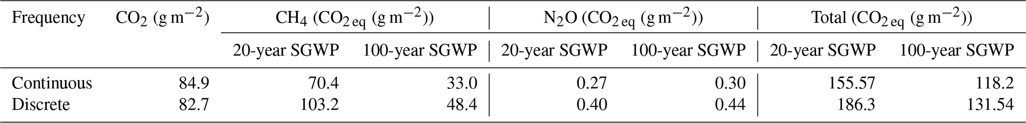
The discrete measurements had a higher SGWP potential than the continuous measurements (Table 2). While the discrete measurements had a slightly lower SGWP for CO₂ and a slightly higher SGWP for N₂O, the difference between continuous and discrete SGWP was driven by CH₄. The 20- and 100-year SGWP for discrete measurements of CH₄ were up to ∼ 38 % higher than the respective continuous measurements, contributing to an overall increase of ∼ 18 % and ∼ 11 % for the discrete measurement's 20- and 100-year SGWP.

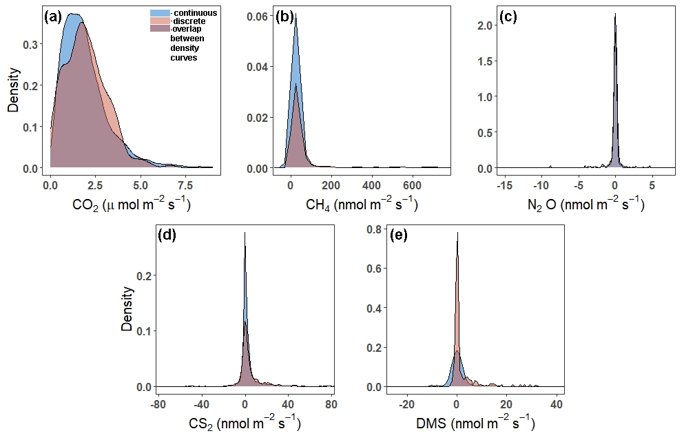
Figure 4 Density plots comparing the distribution of fluxes throughout all campaigns (continuous over ∼ 72 h) to those measured during daytime low tide (discrete, 1 h before and 1 h after daytime low tide) for (a) CO₂, (b) CH₄, (c) N₂O, (d) CS₂, and (e) DMS. Note that the scales on the x- and y axes are different. The tails have been cut off to better see the peaks for (b), (c), (d), and (e). For plots with full distributions, see Fig. S2.

Table 1 Summary of continuous (over ∼ 72 h) and discrete (one hour before and one hour after low tide) measurement data and distributions for each gas. An alpha of < 0.05 was used to determine significant differences between the means and the distributions. Note that the means for CO₂ are in µmol m⁻² s⁻¹, while the other gases are in nmol m⁻² s⁻¹.

4 Discussion

4.1 Measuring all the time: seasonal and diel patterns and hot moments of soil trace gases

Spatial variability between the individual chambers at SS were low, but CO₂ fluxes showed temporal variability that corresponded to changes in temperature. The relatively low spatial variability within our experimental setting contrasts with previously reported high spatial variability of CO₂ fluxes attributed to the presence of a hot spot (Capooci and Vargas, 2022a). However, previous CO₂ fluxes measured at the SS site ranged from 0–15 µmol m⁻² s⁻¹, with the bulk of the measurements between 0 and 5 µmol m⁻² s⁻¹, with higher fluxes associated with hot spots or warmer temperatures (Capooci and Vargas, 2022a; Seyfferth et al., 2020; Hill and Vargas, 2022). Therefore, location of measurements within a landscape could be influenced by hot spots, which complicates ecosystem scale calculations of soil CO₂ fluxes (Barba et al., 2018). In addition, there was a seasonal pattern evident in the CO₂ fluxes, with higher emissions during the growing season, as is typical in temperate ecosystems, as well as in the significant relationship between CO₂ and air temperature. Within salt marshes, soil organic matter decomposition into products such as CO₂ correlates with temperature due to the activation energy needed for organic matter breakdown (McTigue et al., 2021). Other studies at temperate wetland sites have found higher fluxes during the summer (Simpson et al., 2019; Yu et al., 2019; Bridgham and Richardson, 1992), as well as relationships between CO₂ fluxes and temperature (Capooci and Vargas, 2022a; Simpson et al., 2019; Xie et al., 2014) highlighting that CO₂ fluxes in temperate salt marshes exhibit a temperature dependency over seasonal scales, even in the presence of tides.

While CO₂ fluxes show seasonal patterns, there are no diel patterns that persist throughout the year. During G1, the peak of high tide coincided with peak daily temperature. This scenario also occurred during D1, but fluxes were too low to discern patterns. During all other campaigns, low tide and peak temperatures coincided. These results suggest that diel patterns may occur periodically under certain conditions. For example, at the SS site, it may be that diel patterns occur during high tide at the temperature peak. While we expected the highest fluxes during low tides due to increased oxygen exposure, there may be a lag between low tide in the creek and low water levels at the SS site, resulting in higher fluxes during high tide in the creek. However, these results can vary from site to site and with proximity to the tidal creek. More research using high temporal frequency measurements are needed to parse out the role of temperature and tides on CO₂ fluxes across salt marshes to properly represent the pattern in earth system models (Ward et al., 2020).

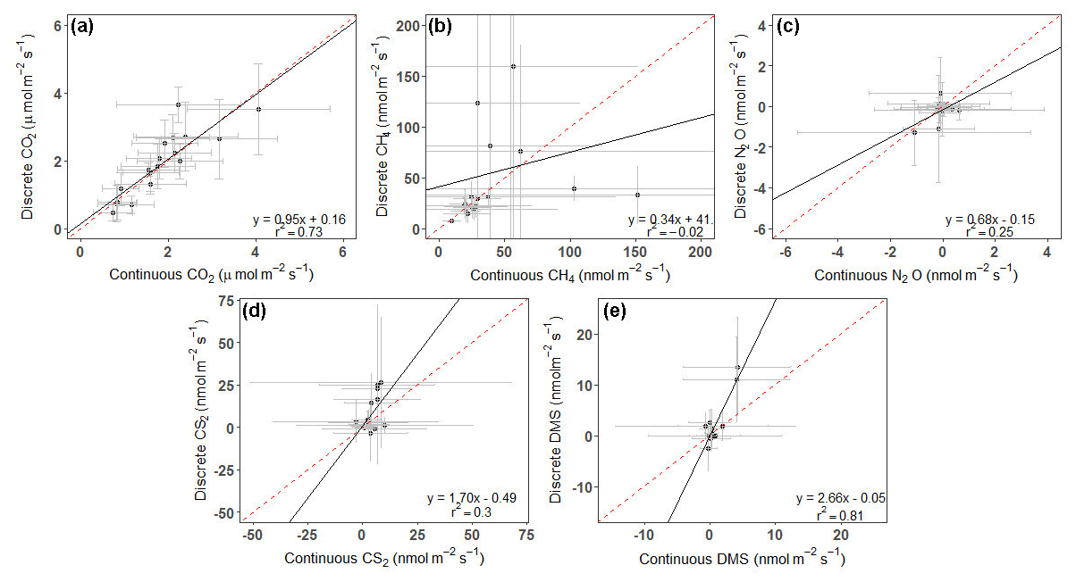
Figure 5 Plots comparing the daily average of continuous (over ∼ 72 h) to discrete (1 h before and 1 h after daytime low tide) measurements for (a) CO₂, (b) CH₄, (c) N₂O, (d) CS₂, and (e) DMS. Error bars represent the SD and have been cut off in panel (b) to show data better. See Fig. S3 for full error bars for panel (b). Dashed red line is the 1:1 line, while the solid black line is the trend line.

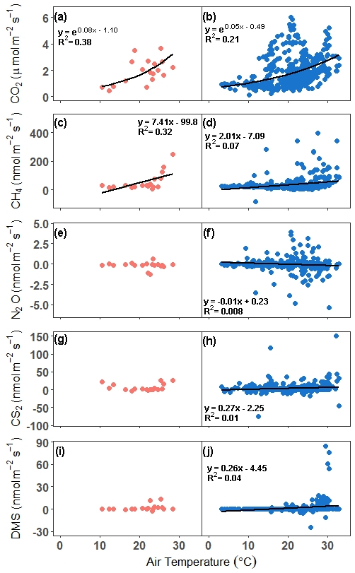
Figure 6 Comparison of fluxes versus air temperature for all campaigns. In panels (a), (c), (e), (g), and (i), the discrete (1 h before and 1 h after daytime low tide) daily mean is compared with the daily mean air temperature, while in panels (b), (d), (f), (h), and (j), the hourly continuous (over ∼ 72 h) mean is compared with the hourly air temperature. The trend lines for significant relationships at alpha < 0.05 are plotted. Note that in panel (d), the outlier hourly mean of 2275 nmol m⁻² s⁻¹ is not included in the trend line or in the graph.

Similarly to CO₂, CH₄ has a significant relationship with air temperature; however, it explains less variability in the fluxes. Several studies have found positive correlations between soil CH₄ fluxes and temperature (Bartlett et al., 1985; Emery and Fulweiler, 2014; Wang and Wang, 2017) in temperate salt marshes, while others have not (Wilson et al., 2015). It is important to note that while, in general, salt marsh CH₄ fluxes are positively related to temperature (Al-Haj and Fulweiler, 2020), the ability of temperature to explain CH₄ flux variability is low, compounded by many, often site-specific, factors that affect methane production and consumption, such as organic matter supply, microbial communities, and diffusion rates (Al-Haj and Fulweiler, 2020; Bartlett et al., 1985).

At our study site, CH₄ fluxes were highest and pulses were most frequent during senescence, agreeing with findings from ecosystem-scale measurements derived using the eddy covariance technique (Vázquez-Lule and Vargas, 2021). In most wetland ecosystems, including those in northern, temperate, and subtropical areas, the highest fluxes have been reported during the summer (Kim et al., 1998; Rinne et al., 2007; Van Der Nat and Middelburg, 2000; Livesley and Andrusiak, 2012; Turetsky et al., 2014), but we highlight that there is a lack of measurements during the winter (Al-Haj and Fulweiler, 2020). In S. alterniflora marshes, highest mean CH₄ fluxes have been found in both the summer and the fall (Bartlett et al., 1985; Emery and Fulweiler, 2014). At a site dominated by S. alterniflora, both high fluxes and pore water CH₄ concentrations were found in September (Zhang and Ding, 2011), indicating either a continual buildup of CH₄ in the pore water over the growing season and/or increased CH₄ production in the fall. For our site, it is likely that higher CH₄ emissions during senescence were due to an input of labile organic matter from plant die-off (Seyfferth et al., 2020). Furthermore, a recent study has shown that pore water DMS, a non-competitive substrate for methylotrophic methanogenesis that is produced from the breakdown of DMSP, a metabolite produced by S. alterniflora (Dacey et al., 1987), peaks during the fall (Tong et al., 2018). Therefore, we postulate that an influx of DMS may also contribute to higher CH₄ fluxes during senescence in marshes dominated by S. alterniflora. This finding highlights the importance of carbon–sulfur biogeochemistry and measuring fluxes during non-summer months, particularly in marshes that have plant communities that provide substrates used in methylotrophic methanogenesis (Seyfferth et al., 2020).

Table 2 Sustained global warming potential (SGWP) derived from continuous (over ∼ 72 h) and discrete (1 h before and 1 h after daytime low tide) temporal measurements in a tidal salt marsh.

On a diel timescale, pulse emissions of CH₄ from the soil tend to occur during the warmest time of the day, as well as during low and rising tides. There are very few studies that report high temporal frequency data of CH₄ emissions, most of which include plants within their scope (via transparent chambers or eddy covariance) or focus on tidal creeks, making it difficult to ascertain whether the diel patterns seen in this study are typical of tidal salt marsh soils. Of the studies that report high temporal frequency data of plant- or water-based CH₄ fluxes in coastal vegetated ecosystems, CH₄ emissions have been found to peak at various points in the day, from during the day (Yang et al., 2017, 2018; Tong et al., 2013), at night (Diefenderfer et al., 2018), or highly variable (Jha et al., 2014; Xu et al., 2017). At our site, CH₄ fluxes tended to peak at the confluence of peak daily temperature and low to rising tides, indicating that physical forcing may contribute to CH₄ pulses (Bahlmann et al., 2015; Middelburg et al., 1996). However, pulses did occur during other times throughout the day and within the tidal cycle. While some of the pulse emissions may be a result of ebullition, the majority are associated with high R² levels, indicating that they are sustained over the measurement period. Our results demonstrate the importance of conducting high temporal frequency CH₄ measurements in tidal salt marsh soils for several reasons, including the need for more data to better understand the drivers of CH₄ fluxes at diel scales and how that affects model predictions.

N₂O emissions and uptake loosely followed a seasonal pattern, likely driven by the canopy phenological stages. During the growing season, it has been shown that highly productive plants can compete with soil microbes for NO${}_{\mathrm{3}}^{-}$ and NH${}_{\mathrm{4}}^{-}$ (Cheng et al., 2007; Yu et al., 2012; Zhang et al., 2013; Granville et al., 2021; Xu et al., 2017), shifting denitrifiers into consuming N₂O and resulting in a net uptake during G1 and M1. As the plants reach peak maturity, the system shifts into net emission of N₂O during M2 and S1. One study found that nitrogen additions resulted in a pulse of N₂O in July when most of the plant growth had occurred, but no response in April, suggesting that the competition for NO${}_{\mathrm{3}}^{-}$ and NH${}_{\mathrm{3}}^{+}$ decreases when plant growth has slowed down (Moseman-Valtierra et al., 2011). Increased substrate availability combined with warm temperatures likely contributed to the marsh being a net source of N₂O during the later stages of the growing season. As temperatures drop, the system shifts back into net uptake, as seen during S2 and D1. Similar seasonal patterns have been seen in other studies, albeit shifted by a month or two depending on the local climate and phenophases (Granville et al., 2021; Emery and Fulweiler, 2014). These findings highlight balance between processes that produce N₂O (e.g., nitrification, denitrification, and nitrifier–denitrification) and consume N₂O (e.g., denitrification), as well as substrate availability and plant phenology in determining whether a marsh is a source or sink of N₂O at any given point.

As with seasonality, diel patterns of N₂O showed both emissions and uptake. Several studies have also reported both emissions and uptake during a 24 h period (Yang et al., 2017; Tong et al., 2013). We found that pulses of uptake and emissions occurred both during the day and at night, as well as during different phases of the tidal cycle. Studies have found higher fluxes during the day (Tong et al., 2013; Yang et al., 2017) and at night (Laursen and Seitzinger, 2002; Yang et al., 2017; Bauza et al., 2002). Generally, fluxes were slightly higher at night throughout the campaigns, perhaps as a result of increased availability of NH${}_{\mathrm{4}}^{+}$ at night due decreased competition from photosynthesizers (Bauza et al., 2002). Overall, N₂O fluxes were near zero with a < 0.50 nmol m⁻² s⁻¹ difference between daytime and nighttime mean fluxes, suggesting that N₂O fluxes do not play a major role in GHG emissions at this salt marsh.

Our automated measurements of sulfur-based trace gases show high variability in CS₂, with low fluxes punctuated by occasional pulse emissions. There are no previous studies with automated measurements to compare our findings, but previous studies have noted that CS₂ fluxes are highly variable (Steudler and Peterson, 1985; Hines, 1996), with periods of emission and uptake. However, fluxes at SS were, on average, an order of magnitude higher than values reported in the literature (Table S1 in the Supplement). There could be several reasons for the difference in magnitudes: (1) improvement in instrumentation to detect CS₂, (2) sampling technique differences, and/or (3) site-specific characteristics. Since the influx of sulfur-based trace gas measurements in the 1980s, instrumentation has advanced from using molecular sieves and cryotraps to store samples before measuring them on a gas chromatograph (e.g., Carroll et al., 1986; Cooper et al., 1987a; Steudler and Peterson, 1984) to using portable Fourier transform infrared (FTIR) spectrometers that measure trace gas concentrations in near real time. These instrumentation advances subsequently led to changes in sampling techniques. Traditionally, it was common to keep the chamber closed for upwards of 24 h, with samples being collected over hourly intervals throughout the day (Carroll et al., 1986; Goldan et al., 1987). Sweep air free of sulfur trace gases was also commonly used to avoid the need to take samples at both the inlet and outlets of the chambers (Goldan et al., 1987). However, others used ambient air because it more closely resembled in situ conditions (Steudler and Peterson, 1985). With recent advances, sampling techniques have changed to eliminate the need for very long closure times and reduce the effects the chambers have on micrometeorological conditions. Now, high temporal frequency, long-term data can be obtained, thereby capturing pulse emissions that otherwise may be missed. The third reason for difference in magnitude could be due to site-specific differences in CS₂ fluxes. While the mechanisms by which CS₂ is produced are poorly understood, there are several potential production pathways: OM degradation, photochemical production, and algal production (Xie and Moore, 1999). The most likely pathway for our site is the microbially mediated reaction between H₂S and organic matter due to high sulfur concentrations, anaerobic conditions, and a large pool of decaying organic matter. Finally, CS₂ is a short-lived sulfur gas, but the major product of CS₂ oxidation is COS; consequently, understanding CS₂ production and oxidation is important for recognizing the role of salt marshes in COS dynamics (Whelan et al., 2013).

The mean of measured DMS fluxes generally fall within those reported in the literature but with pulses higher than previously reported and different temporal patterns. We found that DMS fluxes only occurred during the middle of the day, near when air temperatures peaked. This is contrary to several studies that have found DMS fluxes during other times of the day (Morrison and Hines, 1990; Steudler and Peterson, 1985; DeLaune et al., 2002). Some studies have found diel patterns related to temperature (De Mello et al., 1987; Cooper et al., 1987b) and incoming tides (Morrison and Hines, 1990; Dacey et al., 1987; Goldan et al., 1987). Our results indicate that DMS fluxes from the SS site are associated with temperature and light-related processes, whether these variables influence microbial activity, plant physiology, or a combination of both. A study found that DMS fluxes peaked after a full daylight period in a Danish estuary (Jørgensen and Okholm-Hansen, 1985). However, there is no information on the diel patterns of DMS in the sediment pore water or its release from S. alterniflora plants. DMS is also produced by other pathways that occur under anoxic conditions, such as methylation of sulfide and methanethiol (Lomans et al., 2002; Sela-Adler et al., 2015), microbial reduction of dimethylsulfoxide (Capone and Kiene, 1988), and/or the incorporation of inorganic substrates (i.e., CO₂) and organic methylated compounds (Finster et al., 1990; Moran et al., 2008; Lin et al., 2010). To better understand DMS fluxes, more research into the dynamics between S. alterniflora, pore water DMS, and DMS fluxes is needed, as it plays an important role in carbon–sulfur biogeochemistry, particularly as a non-competitive substrate for methylotrophic methanogenesis (Seyfferth et al., 2020).

4.2 Continuous versus discrete measurements: Do we get the same information?

Our results show that discrete temporal measurements of CO₂ during daytime low tide throughout the year (including dormancy) may be sufficient to obtain a representative mean of the temporal variability of soil CO₂ flux. This has implications for calculating carbon budgets. Furthermore, the distribution of continuous and discrete CO₂ fluxes is similar, indicating that discrete measurements are capturing variability similar to that of continuous measurements. This observation is reinforced by the CO₂ ∼ air temperature relationships, which do not have significantly different slopes (discrete: 0.03–0.12; continuous: 0.04–0.05), providing further support for the utility of daytime low tide discrete measurements in evaluating potential drivers of CO₂ variability.

In contrast, high variability in CH₄ fluxes resulted in the means for discrete and continuous measurements to be similar but with significantly different distributions. In salt marshes, CH₄ fluxes are characterized by high variability (Rosentreter et al., 2021), making it difficult to assess the processes that control CH₄ fluxes (Vázquez-Lule and Vargas, 2021). While the means were not significantly different despite ∼ 33 % higher mean flux using discrete measurements, it is important to note that the 95 % confidence interval and the coefficient of variation are broad and very high, resulting in potential error cancellation for the calculation of the mean. We postulate that the discrete measurement approach can be used to calculate budgets with the caveat of large uncertainties and that they likely overestimate the mean CH₄ flux. Discrete measurements do not capture variability similar to that of continuous measurements and have a stronger air temperature-CH₄ flux relationship than continuous measurements, despite the overlap between their confidence intervals (2.14–12.7 and 1.31–2.71, respectively). However, continuous measurements provide a more accurate depiction of the patterns and magnitudes of CH₄ and can provide stronger insights into the interrelated drivers of CH₄ fluxes.

Regardless of the sampling interval, N₂O fluxes had means that were near zero. Due to fluxes consistently being near zero, the discrete and continuous measurements will likely get similar overall results due to error cancellation even if the distributions were significantly different. The continuous measurements capture a wider range of fluxes than the discrete measurements, as seen with their very high coefficient of variance and different distribution. However, the skewness between the two approaches is very similar, due to the bulk of the measurements falling around the same values as seen in the large amount of overlap in the density curves. It is important to note that this site is nitrogen limited, which constrains N₂O production. In marshes that are not nitrogen limited, sampling intervals will likely play a more important role since fluxes will be higher.

For CS₂, discrete and continuous measurements did not have similar means or distributions, likely due to the high variability found in these measurements. Previous studies using discrete measurements of CS₂ have noted its high variability (e.g., De Mello et al., 1987), with one highlighting the need for frequent measurements of sulfur-based trace gases during the day in order to obtain an accurate mean daily flux value (Steudler and Peterson, 1985). We found that discrete measurements taken during daytime low tide result in a daily mean that is nearly twice that of the daily mean from continuous measurements. The average CS₂ fluxes measured during our field campaigns were up to an order of magnitude higher than previously reported. We advocate for more measurements of CS₂ fluxes beyond focusing on low tide windows and during different canopy phenological phases across salt marshes to better understand the dynamics of this trace gas.

When measuring DMS fluxes during daytime low tide, the mean is similar to the continuous measurement mean, but the distributions are significantly different. However, caution should be taken in using discrete measurements of DMS to calculate daily means, particularly if those measurements fall during the warmest part of the day when DMS fluxes are the most active. This could result in overestimating the daily mean since extended periods of no fluxes are not accounted for. One approach to measuring DMS fluxes would be to use the strong relationship between discrete and continuous measurements to correct for the overestimation of discrete fluxes. However, this approach would still require the use of a continuous, automated system at different points throughout the year to establish a site-specific correction of discrete mean DMS fluxes, particularly if DMS fluxes are used to calculate DMS budgets.

5 Conclusion: what we may be missing and challenges

Discrete measurements have the clear advantage of capturing the spatial variability of soil trace gas fluxes across an ecosystem, but this approach is also used to describe the temporal variability. In contrast, continuous measurements using autochambers accurately describe temporal patterns (e.g., hourly measurements) but have limited spatial representation due to high instrumentation costs and limited spatial extent of the area where autochambers can be deployed (Vargas et al., 2011; Barba et al., 2018). Here we discuss the advantages and differences from discrete and continuous measurements derived from this study.

Discrete measurement campaigns are suitable for calculating budgets, particularly for CO₂ and N₂O since they capture comparable means. While we found that CH₄ and DMS means were not significantly different between the two approaches, there are caveats that must be considered when using discrete measurements. The high variability inherent in CH₄ fluxes can contribute to the lack of significant differences between the two approaches and result in discrete measurements overestimating the overall CH₄ fluxes from a tidal salt marsh. This has implications when calculating SGWP where differences in CH₄ means largely contribute to the differences in SGWP between the two approaches and can affect how scientists and policymakers view tidal salt marshes and blue carbon as a natural climate solution (Macreadie et al., 2021). For DMS, it is important to assess diel patterns to ensure that fluxes are representative, particularly at sites that have patterns similar to what is seen at our study site.

When evaluating variability or trying to parse out the processes that drive GHG and trace gas emissions from tidal salt marshes (e.g., functional relationships), using continuous, automated measurements would be the best approach. This is particularly important for CH₄, where pulse emissions are frequent during the growing season and can be very high. Using continuous measurements is also important in scenarios where discrete measurements do not capture a similar mean or distribution, as with CS₂ fluxes. We recognize that continuous measurements are expensive and difficult to implement across study sties, but we advocate for revisiting monitoring protocols and identifying potential biased interpretation of trace gas flux information from discrete measurements. Discrete measurements are more capable of representing spatial variability, and until we have a better understanding of which source of variability is higher, temporal or spatial, both techniques should be considered for ecosystem assessments.