the Creative Commons Attribution 4.0 License.
the Creative Commons Attribution 4.0 License.
 | 28 Jan 2022
Spatially varying relevance of hydrometeorological hazards for vegetation productivity extremes
Jasper M. C. Denissen
Mirco Migliavacca
Wantong Li
Anke Hildebrandt
Rene Orth
Vegetation plays a vital role in the Earth system by sequestering carbon, producing food and oxygen, and providing evaporative cooling. Vegetation productivity extremes have multi-faceted implications, for example on crop yields or the atmospheric CO2 concentration. Here, we focus on productivity extremes as possible impacts of coinciding, potentially extreme hydrometeorological anomalies. Using monthly global satellite-based Sun-induced chlorophyll fluorescence data as a proxy for vegetation productivity from 2007–2015, we show that vegetation productivity extremes are related to hydrometeorological hazards as characterized through ERA5-Land reanalysis data in approximately 50 % of our global study area. For the latter, we are considering sufficiently vegetated and cloud-free regions, and we refer to hydrometeorological hazards as water- or energy-related extremes inducing productivity extremes. The relevance of the different hazard types varies in space; temperature-related hazards dominate at higher latitudes with cold spells contributing to productivity minima and heat waves supporting productivity maxima, while water-related hazards are relevant in the (sub-)tropics with droughts being associated with productivity minima and wet spells with the maxima. Alongside single hazards compound events such as joint droughts and heat waves or joint wet and cold spells also play a role, particularly in dry and hot regions. Further, we detect regions where energy control transitions to water control between maxima and minima of vegetation productivity. Therefore, these areas represent hotspots of land–atmosphere coupling where vegetation efficiently translates soil moisture dynamics into surface fluxes such that the land affects near-surface weather. Overall, our results contribute to pinpointing how potential future changes in temperature and precipitation could propagate to shifting vegetation productivity extremes and related ecosystem services.
- Article
(7588 KB) - Full-text XML
-
Supplement
(15435 KB) - BibTeX
- EndNote


Vegetation is a crucial component of the Earth system because it provides ecosystem services like food and oxygen production, CO2 sequestration and evaporative cooling. Therefore, the effects of changes in vegetation productivity are diverse; it influences crop yields (Orth et al., 2020), cloud formation (Hong et al., 1995; Freedman et al., 2001), precipitation (Pielke et al., 2007), atmospheric pollution (Otu-Larbi et al., 2020) and heat wave intensity (J. Li et al., 2021).
Photosynthesis requires a sufficient water (soil moisture) and energy (incoming short-wave radiation) supply. In regions that are water-limited (energy-limited), plants usually benefit from water (energy) surpluses and suffer from respective deficits. Many studies confirm that, depending on the evaporative regime, vegetation productivity follows the temporal evolution of influential variables such as soil moisture or temperature which summarize the water or energy dynamics (Beer et al., 2010; Seddon et al., 2016; Madani et al., 2017; Orth, 2021; Denissen et al., 2020; Piao et al., 2020; W. Li et al., 2021).
Correspondingly, hydrometeorological hazards, such as temperature and precipitation extremes, have implications on vegetation productivity. Many studies investigated the influence of such hazards on vegetation productivity, highlighting their impact on the biosphere (Ciais et al., 2005; Zhao and Running, 2010; Zscheischler et al., 2013, 2014a, b; Flach et al., 2018; Wang et al., 2019; Zhang et al., 2019; Qiu et al., 2020). However, usually these studies focus on particular types of hydrometeorological hazards such as droughts or heat waves, or they use vegetation productivity data from models or other proxies rather than the recent satellite-derived Sun-induced chlorophyll fluorescence (SIF) data (Frankenberg et al., 2011; Joiner et al., 2013).
In this study, we re-visit the relationship between vegetation productivity and hydrometeorological hazards by analysing the implications of both single and compound hazards on vegetation productivity extremes, as has been highlighted before (Sun et al., 2015; Zhou et al., 2019). However, to our knowledge for the first time, we do so comprehensively by approximating variable importance during vegetation productivity extremes inferred from SIF data on a global scale. This analysis is done from an impact perspective; we first detect impacts (productivity extremes) before relating them to coinciding, potentially extreme hydrometeorological anomalies (Smith, 2011). Finally, we investigate where the full vegetation productivity range between minima and maxima involves transitions from energy to water controls. In regions where this occurs, the feedback of the land surface on the climate can be stronger, as the water-controlled vegetation translates soil moisture dynamics through its energy and water fluxes to affect the boundary layer and consequently also near-surface weather. Hence, our vegetation-based analysis can indicate hotspots of land–atmosphere coupling (Koster et al., 2004; Guo and Dirmeyer, 2013).
In Sect. 3.1 we investigate the co-occurrence of vegetation productivity extremes and hydrometeorological hazards. Further, we show the timing of such vegetation productivity extremes in Sect. 3.2. Additionally, we determine the main drivers of vegetation productivity extremes and assess the influence of underlying evaporative regimes in Sect. 3.3. We summarize our results across climate regimes in Sect. 3.4 and investigate regions with vegetation productivity controls switching between water and energy variables in Sect. 3.5.
In order to characterize vegetation behaviour, we use SIF and enhanced vegetation index (EVI) data in this study. SIF is used as a proxy for vegetation productivity. We employ satellite-observed SIF data retrieved from the Global Ozone Monitoring Experiment (GOME-2; Köhler et al., 2015). In the derivation of this SIF product, multiple corrections for varying solar zenith angles, differences in overpass times and cloud fraction have been applied to yield reliable SIF estimates. In addition to vegetation productivity, we also study changes related to vegetation greenness by using satellite-observed EVI data from the Moderate Resolution Imaging Spectroradiometer (MODIS; Didan, 2015).
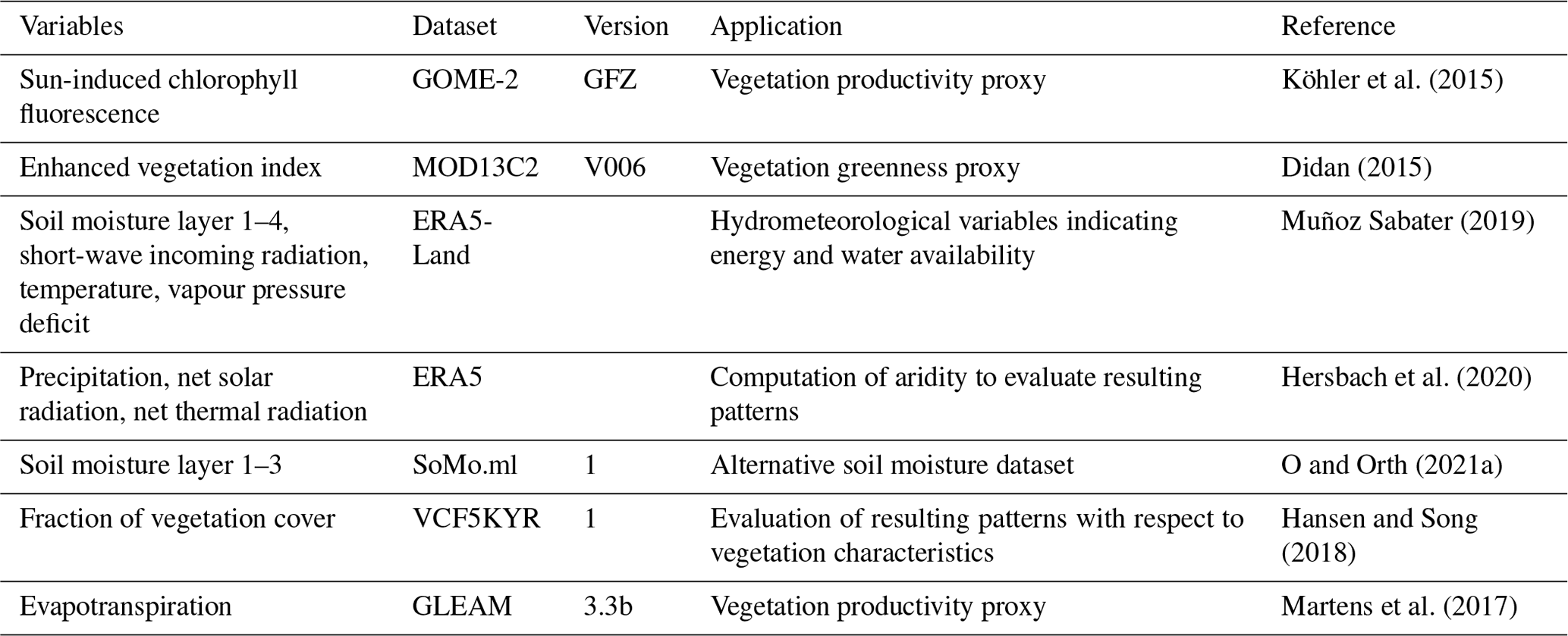
As for the hydrometeorological variables, representing energy and water availability, we consider 2 m temperature, short-wave incoming radiation, vapour pressure deficit, soil moisture from four layers (1: 0–7 cm, 2: 7–28 cm, 3: 28–100 cm and 4: 100–289 cm) and total precipitation, all from the ERA5-Land reanalysis data (Muñoz Sabater, 2019). In addition to this and to validate the robustness of our results, we use an alternative soil moisture product, SoMo.ml, which provides data for three layers (1: 0–10 cm, 2: 10–30 cm and 3: 30–50 cm) and which is derived through a machine learning approach that is trained with in situ soil moisture measurements from across the globe (O and Orth, 2021a). All datasets used in this study are summarized in Table 1.
Table 1Datasets used in this study. GLEAM: Global Livestock Environmental Assessment Model. GFZ: German Research Centre for Geosciences. VCF: vegetation continuous fields.
The workflow applied to these datasets is illustrated in Fig. 1. At first, all data are pre-processed for comparability by (i) aggregating it to monthly 0.5∘ spatial and temporal resolution and by (ii) focusing on the time period 2007–2015. Next, we compute anomalies by removing linear trends and the mean seasonal cycle from the data for both the vegetation and hydrometeorological variables. In each grid cell, we disregard months with an absolute SIF value below 0.5 mW m−2 sr−1 nm−1 to focus on times with sufficiently active vegetation (as in W. Li et al., 2021). Additionally, grid cells with a fractional vegetation cover < 5 % are excluded from the analysis. Finally, we assure the necessary data availability by considering only grid cells with > 15 monthly anomalies across the study period remaining after the filtering. Out of the identified suitable months in each grid cell, we determine the five strongest negative and five strongest positive monthly SIF anomalies. The sum of all grid cells for which five SIF maxima and minima can be detected is referred to as the total study area.
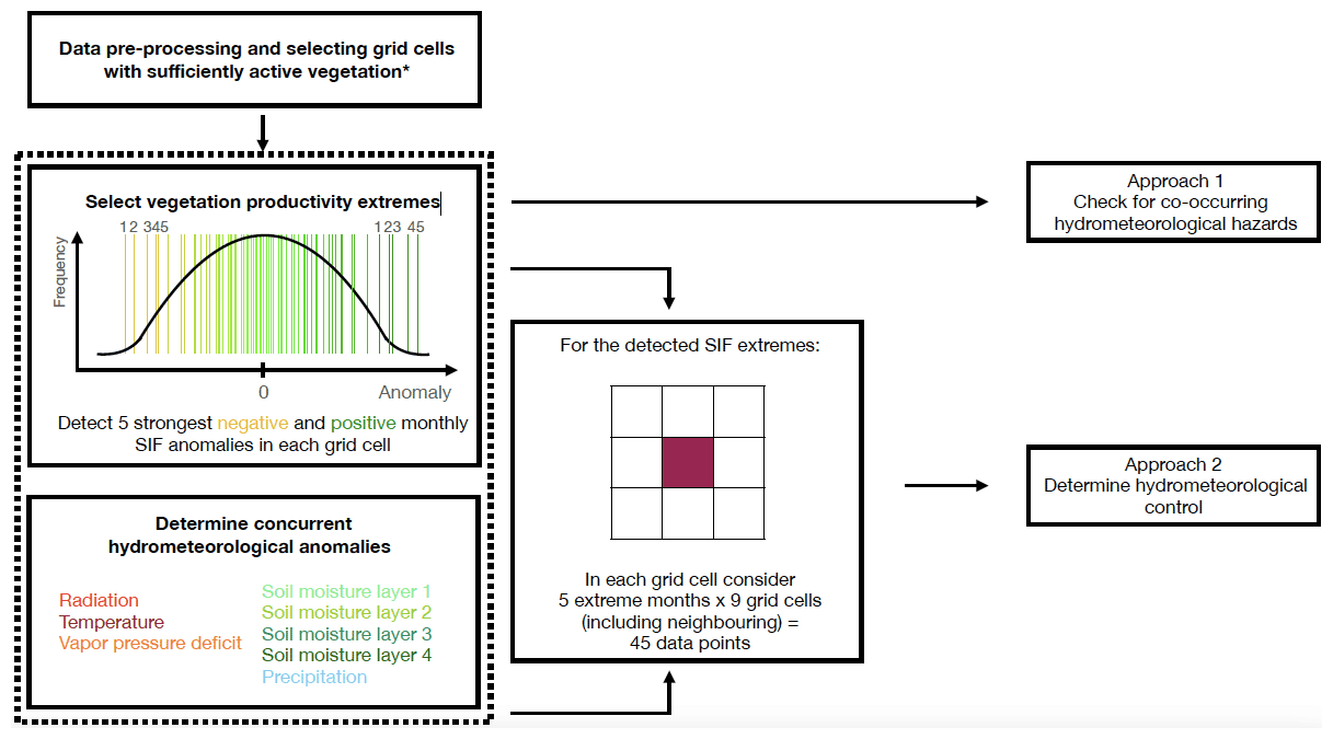
Figure 1Schematic representation of our methodological approach. * Filtering for sufficiently active vegetation is explained in Sect. 2.
After this filtering, we follow two approaches in our analysis. In the first approach, we check for hydrometeorological hazards coinciding with the determined extreme vegetation productivity events. Thereby, we consider air temperature and soil moisture layer 2, as these variables were previously found to be globally most relevant for vegetation productivity (W. Li et al., 2021). At first, we average the monthly temperature and soil moisture anomalies across the 5 months of maximum and minimum SIF anomalies. Then, a series of steps is taken to test if the coinciding hydrometeorological anomalies during SIF extremes are actually hazardous. (i) We randomly sample 5 months with sufficiently active vegetation and average the soil moisture and temperature anomalies, respectively, across them. (ii) We repeat this 100 times to obtain a distribution from which we determine the 10th and 90th percentile. (iii) A hydrometeorological hazard is detected if the actual, averaged temperature and/or soil moisture anomalies associated with the SIF extremes are below the 10th (cold spell or drought) or above the 90th percentile (heat wave or wet spell) of the distribution of randomly sampled averaged anomalies. Note that with this approach we can detect both single and compound hydrometeorological hazards.
Complementing this analysis, in the second approach we analyse the temporal co-variation between SIF extremes and hydrometeorological anomalies. For this purpose, we correlate the five SIF extreme anomalies with anomalies of all considered hydrometeorological variables in each grid cell. We include respective SIF and hydrometeorological data from the surrounding grid cells to yield a larger data sample consisting of data pairs. We disregard negative and insignificant (p value > 0.05) correlations, as we assume these do not indicate actual physical controls but rather represent the influence of noise or confounding effects such as low precipitation during times of high radiation. This also serves to deal with uncertainty in the SIF dataset. When systematic patterns emerge from either of the approaches with adequate significance, they are unlikely confounded by underlying SIF patterns: as we focus solely on either SIF maxima or minima, statistically significant relations only emerge when concurrent hydrometeorological anomalies of an appropriate magnitude exist. Finally, the hydrometeorological variable that yields the highest correlation coefficient with the extreme SIF anomalies is regarded as the main SIF-controlling variable during vegetation productivity maxima or minima.
3.1 Hydrometeorological hazards and vegetation productivity extremes
Figure 2 shows which hydrometeorological hazards are associated with SIF extremes as inferred with approach 1 described in Sect. 2 and in Fig. 1. In approximately 50 % of the global study area, we find that vegetation productivity extremes are associated with hydrometeorological hazards. This is in line with previous research (Zscheischler et al., 2014b). For both maximum and minimum vegetation productivity, we find spatially coherent patterns of associated hydrometeorological hazards. In the Northern Hemisphere, SIF maxima (minima) at high latitudes relate to heat waves (cold spells), where in mid latitudes they occur jointly with wet spells (droughts). This suggests that hydrometeorological hazards associated with SIF extremes vary systematically according to energy and water control of the local vegetation. Thereby, the boundary between both regimes and the respectively determined relevant hydrometeorological hazards is surprisingly sharp, for example in North America and in eastern Europe and Russia (Flach et al., 2018).

Figure 2Hydrometeorological hazards co-occurring with (a) SIF maxima and (b) SIF minima. Colours denote the type of hydrometeorological hazard. Bar plots indicate the area affected by each hazard type relative to the total study area.
Further, single hydrometeorological hazards (either an extreme temperature or soil moisture anomaly) are relevant in more areas than compound hazards (combination of extreme temperature and extreme soil moisture anomaly). Compound hazards seem to be particularly important in the sub-tropics on both hemispheres. Differences also exist between maximum and minimum vegetation productivity extremes, the latter being slightly more associated with compound hazards.
Overall, the most frequent hazards during vegetation productivity minima are droughts and cold spells. Previous studies have reported the relevance of drought in this context (Zscheischler et al., 2013, 2014a, b) even though for different vegetation productivity proxies. On the contrary, the importance of cold spells is not analysed, probably because vegetation productivity in boreal regions is comparably smaller than in e.g. tropical regions (Li and Xiao, 2020).
The results in Fig. 2 are based on averages of the 5 months with strongest SIF anomalies in each grid cell. Figure S1 in the Supplement shows co-occurring hydrometeorological hazards separately for each of the five SIF maxima and minima. The patterns are similar to those in Fig. 2; we consistently find temperature-related hazards to be relevant in energy-controlled regions and water-related hazards in water-controlled regions across all five individual SIF extremes. Weaker SIF extremes tend to be less associated with hydrometeorological hazards. This could be because the signal-to-noise ratio is decreased for weaker extremes, or other factors such as disturbances (fire or insect outbreaks) play a more prominent role for these productivity extremes. As mentioned, soil moisture layer 2 is used here to detect droughts and wet spells, but similar results are obtained with soil moisture layers 1 and 3, respectively (not shown).
3.2 Timing of strongest SIF extremes
To further understand the spatially varying relevance of hydrometeorological hazards, we show the months of the year associated with the strongest SIF extreme in each grid cell in Fig. 3. The spatial pattern is quite different from that in Fig. 2; for example the sharp transitions between regions with energy- and water-related hydrometeorological hazards are not present in Fig. 3. Hence, this transition is apparently not related to SIF extremes occurring in different seasons and might be rather related to different evaporative regimes which will be further investigated in Sect. 3.3. The spatial variability in Fig. 3 is lower at high latitudes compared with (sub-)tropical regions. At high latitudes the growing season is short and constrained by energy availability. In the tropics, we find an increased smaller-scale variability, presumably due to the weak seasonal cycle of hydrometeorological variables. Most SIF extremes in North America and Eurasia occur in the early growing season, presumably when either vegetation starts to grow or growing is limited due to energy or water control. While here we show the months of the year associated with the strongest SIF extreme, in Fig. S2 we show similar patterns in the timing of the second to fifth strongest SIF extremes, indicating that each of the remaining SIF extremes occurs in similar months of the year.
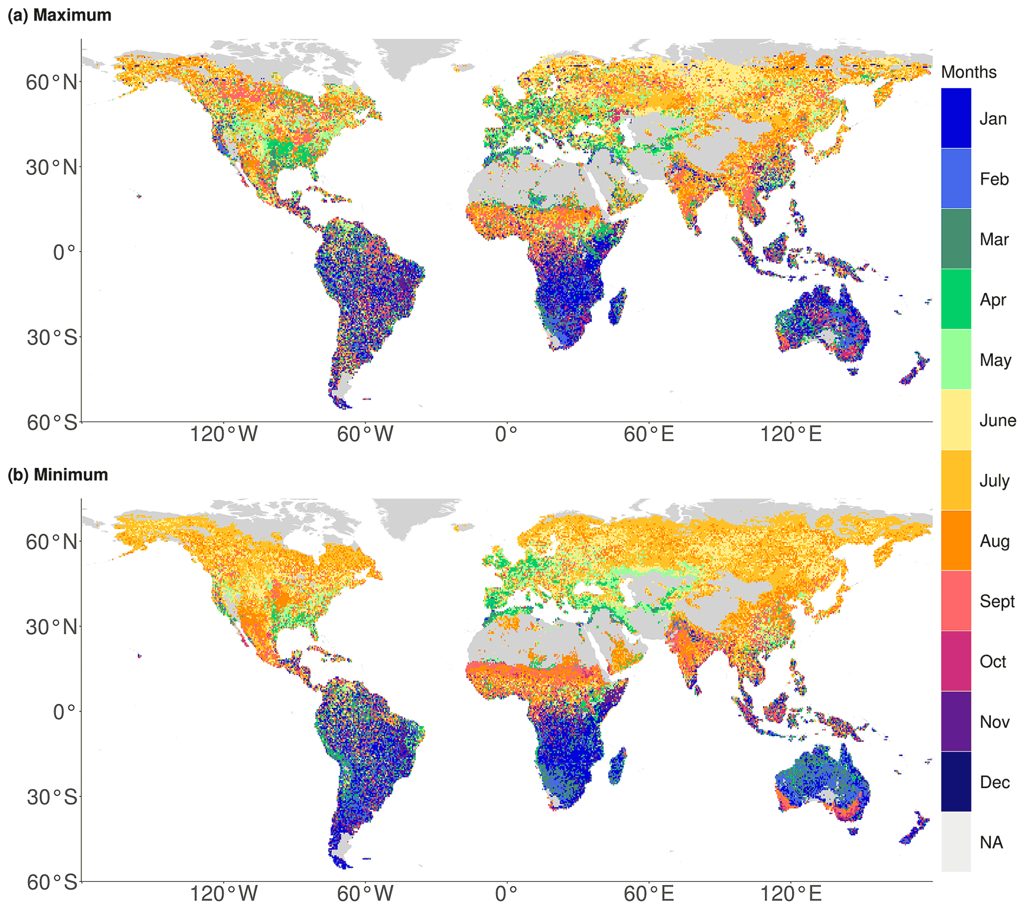
Figure 3Global distribution of the month of the year in which the strongest SIF (a) maximum and (b) minimum anomaly occur. Data gaps (grey) are caused by filtering for active vegetation and excluding insignificant and negative correlations.
3.3 Hydrometeorological drivers of vegetation productivity extremes
After showing the co-occurrence of hydrometeorological hazards with SIF extremes, we apply a correlation analysis (approach 2 in Sect. 2) to characterize the co-variability between extreme SIF anomalies and concurrent hydrometeorological anomalies. Figure 4 shows the hydrometeorological variable that correlates strongest with SIF during months of extreme vegetation productivity, indicating respective controls. At high latitudes and in the tropics SIF extremes are generally energy-controlled, while in the mid latitudes and sub-tropics they are water-controlled. Overall, we find similar spatial patterns as in Fig. 2, demonstrating consistent results across the co-occurrence and co-variability of SIF extremes and hydrometeorological hazards. This coherence suggests that hydrometeorological hazards play a key role in inducing SIF extremes.

Figure 4Global distribution of hydrometeorological controls of Sun-induced chlorophyll fluorescence (SIF) (a) maxima and (b) minima in respective colours, as assessed from the strongest correlations. The inset bar plot indicates the area controlled by each variable relative to the total study area. Dark-grey colour denotes the study area in which correlations are negative/insignificant.
The bar plot insets in Fig. 3 indicate that SIF maxima are equally controlled by energy and water variables, while SIF minima are overall more water-controlled. Even though weaker, this shift is also present in Fig. 2. This difference can be explained with transitional regions, which have energy-controlled SIF maxima but water-controlled SIF minima. This is illustrated for example by the northward shift of the transition between energy and water control in Russia when comparing the results for maximum and minimum SIF. These transitional regions will be further investigated in Sect. 3.5.
We repeated this analysis with SoMo.ml soil moisture and found similar spatial patterns of energy- and water-controlled regions (Fig. S3), underlining that our results are robust with respect to the choice of the soil moisture product. Furthermore, we repeat our co-variability analysis for EVI instead of SIF in Fig. S4, which allows us to contrast to some extent the behaviour of vegetation physiology (SIF) and vegetation structure (EVI). Similar to the spatial patterns of energy- and water-controlled vegetation in Fig. 4, EVI shows predominant energy control at high latitudes, while the mid latitudes are largely water-controlled. Further, as in Fig. 4 for SIF, EVI minima are more associated with water variables than EVI maxima.
However, the overall extent of water-controlled areas is clearly larger in the case of EVI compared with the SIF results. This could (i) be partly related to the fact that EVI, being less dynamic than SIF because it is more related to vegetation greenness and structure, tends to vary at timescales more in line with that of soil moisture (Turner et al., 2020), which can support stronger correlations, or (ii) be due to confounding effects of the changing soil/vegetation colour between dry and wet states on the EVI signal.
3.4 Hydrometeorological controls across climate regimes
In addition to analysing the spatial variation of the main drivers of vegetation productivity extremes, we attempt to further understand the large-scale patterns along temperature and aridity gradients. To this end, we bin grid cells by their climate characteristics as denoted by long-term mean temperature and aridity (the ratio between unit-adjusted net radiation and precipitation). The results in Fig. 5 illustrate which hydrometeorological variable most often has the highest correlation with SIF anomalies in each climate regime.
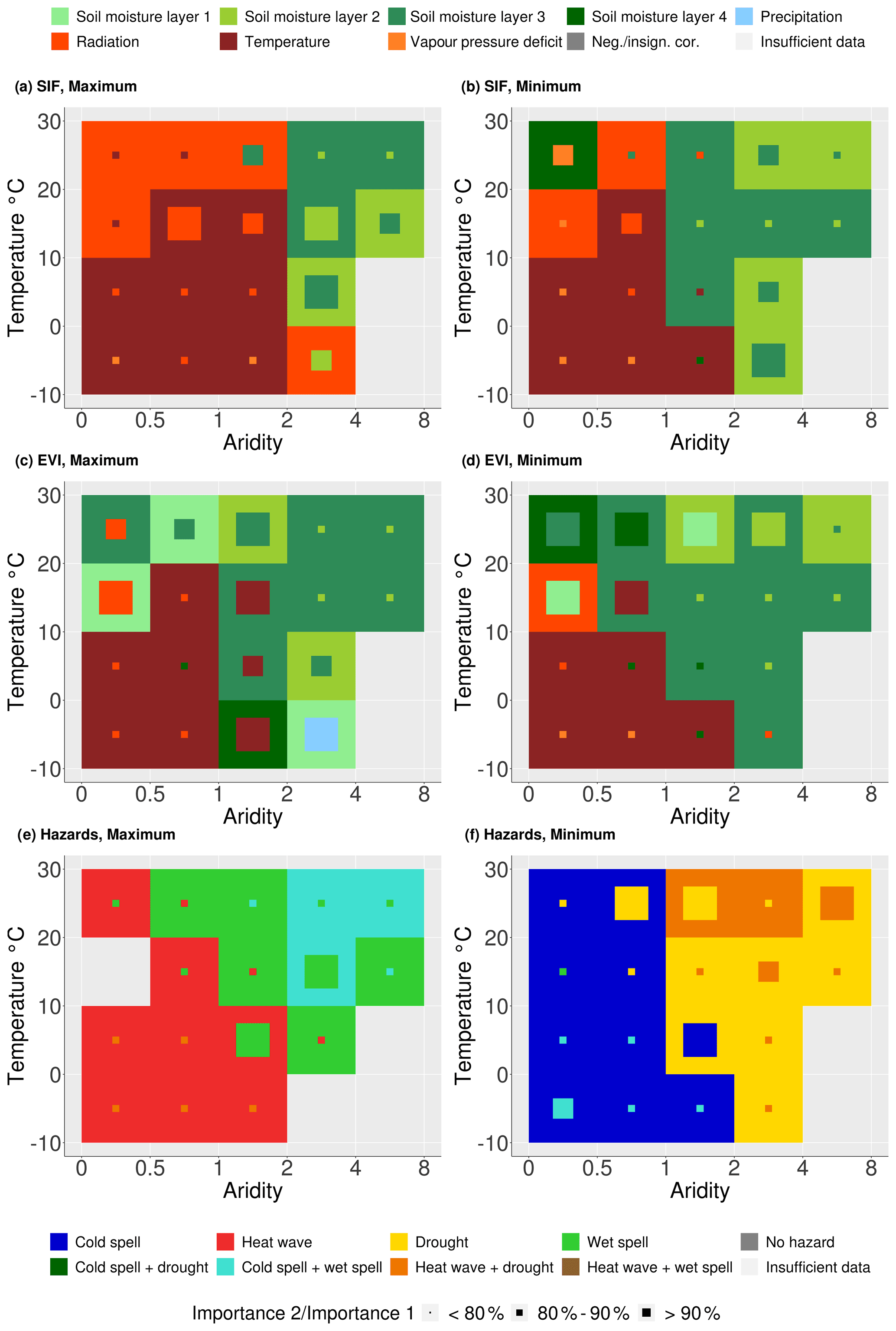
Figure 5Hydrometeorological controls of vegetation productivity extremes summarized across climate regimes: (a, b) Sun-induced chlorophyll fluorescence (SIF) extremes and (c, d) enhanced vegetation index (EVI) extremes. (e, f) Hydrometeorological hazards co-occurring with the SIF extremes. Box colour denotes the main controlling hydrometeorological variable; the second most important variable is indicated in the smaller squares' colour, while its size represents the ratio between the highest and second highest number of grid cells.
Figure 5a and b show that vegetation productivity extremes in humid regions (aridity < 1; Budyko, 1974) are mostly energy-controlled, with temperature controlling in cold regions (long-term average temperature < 10 ∘C) and radiation controlling in warm regions (long-term temperature > 10 ∘C). In contrast, productivity extremes in arid regions (aridity > 2; Budyko, 1974) are mainly water-controlled, with soil moisture layers 2 and 3 as the most important water controls. The main difference between maximum and minimum SIF results is detectable in semi-arid regions (1 < aridity < 2). While for maximum SIF those climate regimes show mostly energy control, SIF minima in these regimes are largely water-controlled. From this, we deduce that semi-arid regions represent the transitional regime, as the main drivers change from energy to water variables from SIF maximum to SIF minimum.
Figure S5 indicates that hydrometeorological anomalies do elicit not only immediate but also lagged vegetation responses. A clear difference between water- and energy-controlled conditions is already visible when correlating hydrometeorological anomalies of the preceding month with the respective SIF extreme. Energy and water surpluses and deficits establish over time, which is most clearly evidenced in arid regions, where precipitation and shallow soil moisture of the preceding month is found to be the most important variable. With time, deeper soil moisture becomes more important (Fig. 5a–b), as in the case of SIF maxima, where precipitation needs time to infiltrate the soil, and in the case of SIF minima, where the soil dries most rapidly from the top down.
The results for EVI show similar patterns despite an increased overall water control as seen earlier in the global maps (Fig. S4). For example, where in humid regions SIF extremes are mainly energy-controlled, EVI extremes are more often water-controlled, which is also reflected in the global maps in Fig. S4.
Figure S6 illustrates similar controlling hydrometeorological variables for SIF and evapotranspiration (ET) extremes. This suggests that carbon and water cycles are sensitive to similar hazards, which in turn enhances their impact on the land climate system via both carbon and water pathways. This further demonstrates the usefulness of SIF observations for reflecting plant transpiration (Jonard et al., 2020). Further, Fig. S6 shows that GLEAM ET extremes relate much more strongly to surface soil moisture than GOME-2 SIF extremes. This could be due to the part of ET that partitions into an unproductive part, bare-soil evaporation, which evaporates water from the surface layer directly, and a productive part, which is connected to carbon uptake and therefore SIF. Surface soil moisture affects the unproductive part while overall enhancing the role of surface soil moisture for ET.
Figure 5e and f show the results of Fig. 2 binned according to their long-term climate characteristics. In humid regions, both SIF extremes are co-occurring with temperature hazards. In contrast, in arid regions water-related hazards co-occur with maximum and minimum SIF. Thereby, Fig. 5 underlines once more the similarity of the results obtained with approaches 1 (Fig. 2) and 2 (Fig. 4).
To additionally explore the influence of different vegetation types and their respective plant physiological differences on the main controls of vegetation productivity, we bin the grid cell results by the respective fraction of tree cover of the entire vegetation cover and by aridity in Fig. S7. We find that the radiation control of SIF extremes in humid regions is mostly associated with forests and that the water control in semi-arid regions largely occurs for shorter vegetation, with presumably more shallow root systems, while productivity extremes in more forested semi-arid regions tend to be energy-controlled. In very strong droughts, tall trees with deep rooting systems are particularly prone to suffer hydraulic failure (Brum et al., 2019). However, in our analysis we consider five events in a 15-year time period such that we likely do not exclusively capture very strong droughts that might results in tree mortality. Generally, hardly any changes in the most important variables can be seen with variations in tree cover, suggesting that on a global scale plant physiological differences only have a limited effect on determining the most important control for SIF extremes. As in Fig. 5, similar patterns are found for EVI extremes with an overall increased relevance of water variables particularly in short vegetation-dominated regions.
3.5 Switching hydrometeorological controls between SIF maxima and minima
In a final step, we focus on shifts between energy and water control when moving from SIF maxima to SIF minima. The respective transitional regions represent hotspots of land–atmosphere coupling such that (i) in these regions the land surface (soil moisture) affects near-surface weather at least during productivity minima (therefore also influencing transpiration) and (ii) this effect can be significant, as transpiration (variability) is relatively high compared with drier regions where vegetation productivity would be water-limited across its entire range from minimum to maximum. The results are depicted in Fig. 6, which illustrates these emerging transitions from water to energy control (yellow) and vice versa (blue, denoting land–atmosphere hotspots). Grid cells that stay within water or energy control, even with a change between the water or energy variables, respectively, are shown in black, indicating no transition. Figure 6a reveals many regions with no transition. Transitions are found mostly in northern Eurasia and North America. Globally, a change from energy control during maximum SIF to water control during minimum SIF occurs more often (7 % of the study area) than the opposite transition (4 %).
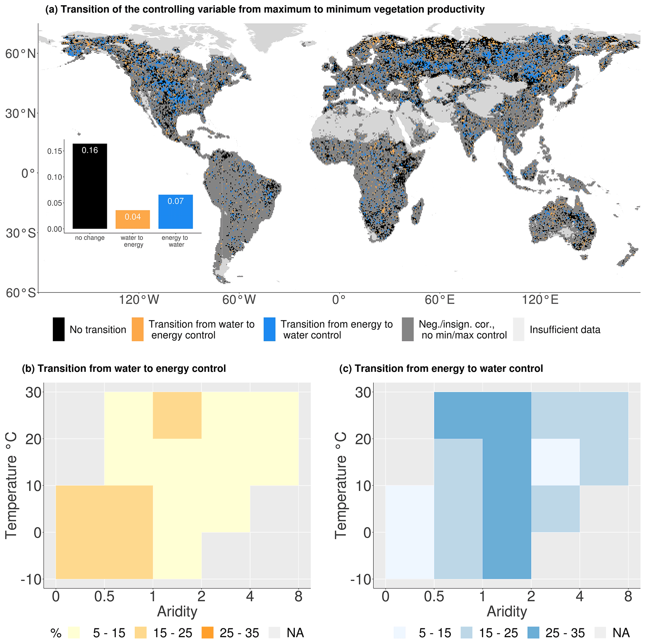
Figure 6Changing hydrometeorological controls between vegetation productivity maxima and minima. (a) Global distribution of changing controls: in panels (b) and (c) grid cells are binned by their long-term climate characteristics. Panel (b) indicates the percentage of grid cells in each climate regime switching from water to energy control; panel (c) denotes the percentage of grid cells changing from an energy-controlled maxima to a water-controlled minima.
Figure 6b and c display the percentage of grid cells in each climate regime changing from water to energy control and vice versa with grid cells binned with respect to long-term climate conditions, similar to Fig. 5. The highest fraction of grid cells in each climate regime would show no change, but as we focus on transitioning grid cells, only they are displayed. Transitions from water to energy control between SIF maxima and SIF minima happen most often in cold, humid regions. This deviates from the prevailing energy control in these climate regimes and is probably related to local-scale features and/or micro-meteorological conditions. Figure 6c indicates that changes from energy control during maximum SIF to water control during minimum SIF most frequently occur in the semi-arid transitional regions. These are land–atmosphere coupling hotspots as described above. The transition from energy to water limitation could be caused by energy-controlled maxima in spring, when presumably soil water resources are available after being replenished during autumn and winter. With sufficient water supply, energy surpluses could induce vegetation productivity maxima. During summer, soil moisture could be depleted for example by the high vegetation demand and therefore take over the SIF control of photosynthesis that is reflected into the SIF dynamics.
3.6 Limitations
Our results are obtained at and valid for relatively large spatial (0.5∘) and temporal (monthly) scales. Previous studies have shown differences in the vegetation–climate coupling across scales (Linscheid et al., 2020), suggesting it would be worthwhile to repeat our analysis for different spatiotemporal scales in the future, possibly with new satellite data products. In this context it should be noted, however, that while the relationship between SIF and gross primary productivity (GPP) as actual vegetation productivity is strong for large spatiotemporal scales (Frankenberg et al., 2011; Guanter et al., 2012; Joiner et al., 2013), it can deteriorate towards smaller scales (He et al., 2020; Magney et al., 2020; Maguire et al., 2020; Marrs et al., 2020; Wohlfahrt et al., 2018). The spatiotemporal range within which there is an acceptable SIF–GPP relationship is not entirely clear yet.
As a second source of uncertainty, SIF data with their relatively large spatial footprint are more vulnerable to cloud contamination compared to finer-scale satellite products (Joiner et al., 2013). Also, especially across South America the SIF data quality is decreased to additional noise (Joiner et al., 2013; Köhler et al., 2015). In our study, many grid cells in these regions and other tropical, cloud-dominated regions exhibit insignificant or negative correlations between SIF and hydrometeorological anomalies, which is why no hydrometeorological controls can be determined there (Fig. 4). Confirming the validity of our results for the tropical grid cells where results can be obtained, we find mostly consistent and physically meaningful results, e.g. radiation being a main driver of vegetation productivity, as the cloud cover limits radiation (reported similarly for non-extreme conditions by Green et al., 2020, and W. Li et al., 2021).
Next to the SIF data, there is also noteworthy uncertainty in the soil moisture data from ERA5. While data quality of surface soil moisture benefits from (satellite) data assimilation, the soil moisture dynamics in deeper layers are more model-based, which somewhat contradicts the observational character of our study. Therefore, we use soil moisture data from SoMo.ml as an independent dataset, which is not based on physical modelling and the related assumptions and parameterizations, as it is derived with machine learning applied to in situ measurements from different depths. Overall, the similar results obtained with ERA5-Land and SoMo.ml soil moisture confirm the robustness of our results despite uncertainties in the soil moisture data.
Finally, the use of correlation methods for inferring causal relations is potentially insufficient and under debate (Krich et al., 2020). We want to emphasize that in our study when referring to “drivers” or “controls” of vegetation productivity, we simply base this on correlation and do not imply causality. Nevertheless, we try to filter out confounding effects by disregarding negative and insignificant correlations. Additionally, testing our methodology (approach 2) for non-anomalous vegetation productivity (Fig. S8), which allows for comparing results with those of W. Li et al. (2021), reveals similar results, while they use a different methodology based on random forests and Shapley Additive Explanations (SHAP) values, which are more robust against confounding effects. Next to this, in our study we apply two different methodologies in approaches 1 and 2 and find similar results, further underlining the robustness of our conclusions.
In this observation-based study, we quantify that vegetation productivity extremes are related to hydrometeorological hazards in about 50 % of the global land area that is sufficiently vegetated and cloud-free. The most relevant hazards for vegetation productivity extremes vary along climate gradients. For vegetation productivity maxima the most relevant hydrometeorological extremes are heat waves in northern latitudes above 50∘ N and wet spells in latitudes below 50∘ N. For productivity minima, drought and cold spells are globally most detrimental to large-scale photosynthesis and carbon uptake. The results of our impact-centric analysis are similar to and complement more traditional climate-centric studies (Ciais et al., 2005; Flach et al., 2018; Qiu et al., 2020). Compound extremes also play a role in 15 %–20 % of our study area; they are somewhat more relevant for productivity minima than for the maxima, with joint drought–heat extremes being most important. Semi-arid, grass-dominated ecosystems tend to transition between water and energy control within the range of their productivity variability. This results in a sensitivity to both water- and energy-related hazards. Thereby, we illustrate how global land–atmosphere coupling hotspots (Koster et al., 2004), where the land surface affects near-surface weather, can be verified using novel vegetation productivity data.
Overall, this study highlights the profound role of (compound) hydrometeorological hazards for global vegetation productivity extremes. Understanding these complex, climate-dependent relationships with present-day observational data is a starting point to more reliably foresee respective changes in a changing future climate with e.g. fewer cold spells but probably more droughts.
All the code used for this analysis is available from the corresponding author upon reasonable request.
The details of all the data used in this study are summarized in Table 1. SIF data are available from GOME-2 (ftp://ftp.gfz-potsdam.de/home/mefe/GlobFluo/GOME-2/gridded, Köhler et al., 2015). EVI (Didan, 2015) and VCF (Hansen and Song, 2018) data can be obtained freely from the NASA EOSDIS Land Processes DAAC (https://doi.org/10.5067/MODIS/MOD13C1.006 and https://doi.org/10.5067/MEaSUREs/VCF/VCF5KYR.001). ERA5-Land soil moisture layers 1–4, short-wave incoming radiation, temperature and vapour pressure deficit and ERA5 precipitation, net solar radiation and net thermal radiation described by Hersbach et al. (2020) are freely available from the Copernicus Climate Change Service (C3S) Climate Data Store (CDS) (ERA5-Land: https://doi.org/10.24381/cds.68d2bb30, Muñoz Sabater, 2019; ERA5: https://doi.org/10.24381/cds.f17050d7, Hersbach et al., 2019). The SoMo.ml dataset as described by O and Orth (2021a) is accessible at https://doi.org/10.6084/m9.figshare.c.5142185.v1 (O and Orth, 2021b). ET data from GLEAM can be obtained from https://www.gleam.eu/#downloads (Martens et al., 2017).
The supplement related to this article is available online at: https://doi.org/10.5194/bg-19-477-2022-supplement.
RO, JMCD and JK jointly designed the study. JK and JMCD performed the analysis. All authors contributed to the writing of the paper, the discussion and interpretation of the results.
The contact author has declared that neither they nor their co-authors have any competing interests.
Publisher’s note: Copernicus Publications remains neutral with regard to jurisdictional claims in published maps and institutional affiliations.
The authors thank Ulrich Weber for help with obtaining and processing the data. Wantong Li acknowledges funding from a PhD scholarship from the China Scholarship Council. Jasper M. C. Denissen, Josephin Kroll and Rene Orth acknowledge funding by the German Research Foundation (Emmy Noether grant no. 391059971).
This research has been supported by the Deutsche Forschungsgemeinschaft (grant no. 391059971).
The article processing charges for this open-access publication were covered by the Max Planck Society.
This paper was edited by Ivonne Trebs and reviewed by two anonymous referees.
Beer, C., Reichstein, M., Tomelleri, E., Ciais, P., Jung, M., Carvalhais, N., Rödenbeck, C., Altaf Arain, M., Baldocchi, D., Bonan, G. B., Bondeau, A., Cescatti, A., Lasslop, G., Lindroth, A., Lomas, M., Luyssaert, S., Margolis, H., Oleson, K. W., Roupsard, O., Veenendaal, E., Viovy, N., Williams, C., Woodward, F. I., and Papale, D.: Terrestrial gross carbon dioxide uptake: global distribution and covariation with climate, Science, 329, 834–838, https://doi.org/10.1126/science.1184984, 2010.
Brum, M., Vadeboncoeur, M. A., Ivanov, V. Asbjornsen, H. Saleska, S., Alves, L. F., Penha, D., Dias, J. D., Aragão, L. E. O. C., Barros, F., Bittencourt, P., Pereira, L., and Oliveira, R. S.: Hydrological niche segregation defines forest structure and drought tolerance strategies in a seasonal Amazon forest, J. Ecol., 107, 318–333, https://doi.org/10.1111/1365-2745.13022, 2019.
Budyko, M. I.: Climate and life, Academic Press, New York, p. 508, 1974.
Ciais, P., Reichstein, M., Viovy, N., Granier, A., Ogée, J., Allard, V., Aubinet, M., Buchmann, N., Bernhofer, Chr., Carrara, A., De Noblet, N., Friend, A. D., Friedlingstein, P., Grünwald, T., Heinesch, B., Keronen, P., Knohl, A., Krinner, G., Loustau, D., Manca, G., Matteucci, G., Miglietta, F., Ourcival, J. M., Papale, D., Pilegaard, K., Rambal, S., Seufert, G., Soussana, J. F., Sanz, M. J., Schulze, E. D., Vesala, T., and Valentini, R.: Europe-wide reduction in primary productivity caused by the heat and drought in 2003, Nature, 437, 529–533, https://doi.org/10.1038/nature03972, 2005.
Denissen, J. M., Teuling, A. J., Reichstein, M., and Orth, R.: Critical soil moisture derived from satellite observations over Europe, J. Geophys. Res.-Atmos., 125, e2019JD031672, https://doi.org/10.1029/2019JD031672, 2020.
Didan, K.: MOD13C1 MODIS/terra vegetation indices 16-day L3 global 0.05 Deg CMG V006, LP DAAC – MOD13C1 [data set], https://doi.org/10.5067/MODIS/MOD13C1.006, 2015.
Flach, M., Sippel, S., Gans, F., Bastos, A., Brenning, A., Reichstein, M., and Mahecha, M. D.: Contrasting biosphere responses to hydrometeorological extremes: revisiting the 2010 western Russian heatwave, Biogeosciences, 15, 6067–6085, https://doi.org/10.5194/bg-15-6067-2018, 2018.
Frankenberg, C., Fisher, J. B., Worden, J., Badgley, G., Saatchi, S. S., Lee, J. E., Toon, G. C., Butz, A., Jung, M., Kuze, A., and Yokota, T.: New global observations of the terrestrial carbon cycle from GOSAT: Patterns of plant fluorescence with gross primary productivity, Geophys. Res. Lett., 38, L17706, https://doi.org/10.1029/2011GL048738, 2011.
Freedman, J. M., Fitzjarrald, D. R., Moore, K. E., and Sakai, R. K.: Boundary layer clouds and vegetation–atmosphere feedbacks, J. Climate, 14, 180–197, https://doi.org/10.1175/1520-0442(2001)013<0180:BLCAVA>2.0.CO;2, 2001.
Green, J. K., Berry, J., Ciais, P., Zhang, Y., and Gentine, P.: Amazon rainforest photosynthesis increases in response to atmospheric dryness, Sci. Adv., 6, eabb7232, https://doi.org/10.1126/sciadv.abb7232, 2020.
Guanter, L., Frankenberg, C., Dudhia, A., Lewis, P. E., Gómez-Dans, J., Kuze, A., Suto, H., and Grainger, R. G.: Retrieval and global assessment of terrestrial chlorophyll fluorescence from GOSAT space measurements, Remote Sens. Environ., 121, 236–251, https://doi.org/10.1016/j.rse.2012.02.006, 2012.
Guo, Z. and Dirmeyer, P. A.: Interannual variability of land–atmosphere coupling strength, J. Hyrdrometeorol., 14, 1636–1646, https://doi.org/10.1175/JHM-D-12-0171.1, 2013.
Hansen, M. and Song, X. P.: Vegetation continuous fields (VCF) yearly global 0.05 deg. NASA EOSDIS Land Processes DAAC, 645, LP DAAC – VCF5KYR [data set], https://doi.org/10.5067/MEaSUREs/VCF/VCF5KYR.001, 2018.
He, L., Magney, T., Dutta, D., Yin, Y., Köhler, P., Grossmann, K., Stutz, J., Dold, C., Hatfield, J., Guan, K., Peng, B., and Frankenberg, C.: From the ground to space: Using solar-induced chlorophyll fluorescence to estimate crop productivity, Geophys. Res. Lett., 47, e2020GL087474, https://doi.org/10.1029/2020GL087474, 2020.
Hersbach, H., Bell, B., Berrisford, P., Biavati, G., Horányi, A., Muñoz Sabater, J., Nicolas, J., Peubey, C., Radu, R., Rozum, I., Schepers, D., Simmons, A., Soci, C., Dee, D., and Thépaut, J.-N.: ERA5 monthly averaged data on single levels from 1979 to present, Copernicus Climate Change Service (C3S) Climate Data Store (CDS) [data set], https://doi.org/10.24381/cds.f17050d7, 2019.
Hersbach, H., Bell, B., Berrisford, P., Hirahara, S., Horányi, A., Muñoz Sabater, J., Nicolas, J., Peubey, C., Radu, R., Schepers, D., Simmons, A., Soci, C., Abdalla, S., Abellan, X., Balsamo, G., Bechtold, P., Biavati, G., Bidlot, J., Bonavita, M., De Chiara, G., Dahlgren, P., Dee, D., Diamantakis, M., Dragani, R., Flemming, J., Forbes, R., Fuentes, M., Geer, A., Haimberger, L., Healy, S., Hogan, R. J., Hólm, E., Janisková, M., Keeley, S., Laloyaux, P., Lopez, P., Lupu, C., Radnoti, G., de Rosnay, P., Rozum, I., Vamborg, F., Villaume, S., and Thépaut, J.-N.: The ERA5 global reanalysis, Q. J. Roy. Meteor. Soc., 146, 1999–2049, https://doi.org/10.1002/qj.3803, 2020.
Hong, X., Leach, M. J., and Raman, S.: A sensitivity study of convective cloud formation by vegetation forcing with different atmospheric conditions, J. Appl. Meteorol. Clim., 34, 2008–2028, https://doi.org/10.1175/1520-0450(1995)034<2008:ASSOCC>2.0.CO;2, 1995.
Joiner, J., Guanter, L., Lindstrot, R., Voigt, M., Vasilkov, A. P., Middleton, E. M., Huemmrich, K. F., Yoshida, Y., and Frankenberg, C.: Global monitoring of terrestrial chlorophyll fluorescence from moderate-spectral-resolution near-infrared satellite measurements: methodology, simulations, and application to GOME-2, Atmos. Meas. Tech., 6, 2803–2823, https://doi.org/10.5194/amt-6-2803-2013, 2013.
Jonard, F., De Cannière, S., Brüggemann, N., Gentine, P., Short Gianotti, D. J., Lobet, G., Miralles, D. G., Montzka, C., Pagán, B. R., Rascher, U., and Vereecken, H.: Value of sun-induced chlorophyll fluorescence for quantifying hydrological states and fluxes: Current status and challenges, Agr. Forest Meteorol., 291, 108088, https://doi.org/10.1016/j.agrformet.2020.108088, 2020.
Köhler, P., Guanter, L., and Joiner, J.: A linear method for the retrieval of sun-induced chlorophyll fluorescence from GOME-2 and SCIAMACHY data, Atmos. Meas. Tech., 8, 2589–2608, https://doi.org/10.5194/amt-8-2589-2015, 2015 (data available at: ftp://ftp.gfz-potsdam.de/home/mefe/GlobFluo/GOME-2/gridded, last access: 6 July 2018).
Koster, R. D., Dirmeyer, P. A., Guo, Z., Bonan, G., Chan, E., Cox, P., Gordon, C. T., Kanae, S., Kowalczyk, E., Lawrence, D., Liu, P., Lu, C.-H., Malyshev, S., Mcavaney, B., Mitchell, K., Mocko, D., Oki, T., Oleson, K., Pitman, A., Sud, Y. C., Taylor, C. M., Verseghy, D., Vasic, R., Xue, Y., and Yamada, T.: Regions of strong coupling between soil moisture and precipitation, Science, 305, 1138–1140, https://doi.org/10.1126/science.1100217, 2004.
Krich, C., Runge, J., Miralles, D. G., Migliavacca, M., Perez-Priego, O., El-Madany, T., Carrara, A., and Mahecha, M. D.: Estimating causal networks in biosphere–atmosphere interaction with the PCMCI approach, Biogeosciences, 17, 1033–1061, https://doi.org/10.5194/bg-17-1033-2020, 2020.
Li, J., Tam, C. Y., Tai, A. P., and Lau, N. C.: Vegetation-heatwave correlations and contrasting energy exchange responses of different vegetation types to summer heatwaves in the Northern Hemisphere during the 1982–2011 period, Agr. Forest Meteorol., 296, https://doi.org/10.1016/j.agrformet.2020.108208, 2021.
Li, W., Migliavacca, M., Forkel, M., Walther, S., Reichstein, M., and Orth, R.: Revisiting Global Vegetation Controls Using Multi-Layer Soil Moisture, Geophys. Res. Lett., 48, e2021GL092856, https://doi.org/10.1029/2021GL092856, 2021.
Li, X. and Xiao, J.: Global climatic controls on interannual variability of ecosystem productivity: Similarities and differences inferred from solar-induced chlorophyll fluorescence and enhanced vegetation index, Agr. Forest Meteorol., 288–289, 108018, https://doi.org/10.1016/j.agrformet.2020.108018, 2020.
Linscheid, N., Estupinan-Suarez, L. M., Brenning, A., Carvalhais, N., Cremer, F., Gans, F., Rammig, A., Reichstein, M., Sierra, C. A., and Mahecha, M. D.: Towards a global understanding of vegetation–climate dynamics at multiple timescales, Biogeosciences, 17, 945–962, https://doi.org/10.5194/bg-17-945-2020, 2020.
Madani, N., Kimball, J. S., Jones, L. A., Parazoo, N. C., and Guan, K.: Global analysis of bioclimatic controls on ecosystem productivity using satellite observations of solar-induced chlorophyll fluorescence, Remote Sens.-Basel, 9, 530, https://doi.org/10.3390/rs9060530, 2017.
Magney, T. S., Barnes, M. L., and Yang, X.: On the covariation of chlorophyll fluorescence and photosynthesis across scales, Geophys. Res. Lett., 47, e2020GL091098, https://doi.org/10.1029/2020GL091098, 2020.
Maguire, A. J., Eitel, J. U. H., Griffin, K. L., Magney, T. S., Long, R. A., Vierling, L. A., Schmiege, S. C., Jennewein, J. S., Weygint, W. A., Boelman, N. T., and Bruner, S. G.: On the functional relationship between fluorescence and photochemical yields in complex evergreen needleleaf canopies, Geophys. Res. Lett., 47, e2020GL087858, https://doi.org/10.1029/2020GL087858, 2020.
Marrs, J. K., Reblin, J. S., Logan, B. A., Allen, D. W., Reinmann, A. B., Bombard, D. M., Tabachnik, D., and Hutyra, L. R.: Solar-induced fluorescence does not track photosynthetic carbon assimilation following induced stomatal closure, Geophys. Res. Lett., 47, e2020GL087956, https://doi.org/10.1029/2020GL087956, 2020.
Martens, B., Miralles, D. G., Lievens, H., van der Schalie, R., de Jeu, R. A. M., Fernández-Prieto, D., Beck, H. E., Dorigo, W. A., and Verhoest, N. E. C.: GLEAM v3: satellite-based land evaporation and root-zone soil moisture, Geosci. Model Dev., 10, 1903–1925, https://doi.org/10.5194/gmd-10-1903-2017, 2017 (data available at: https://www.gleam.eu/#downloads, last access: 10 May 2019).
Muñoz Sabater, J.: ERA5-Land monthly averaged data from 1981 to present, Copernicus Climate Change Service (C3S) Climate Data Store (CDS) [data set], https://doi.org/10.24381/cds.68d2bb30, 2019.
O, S. and Orth, R.: Global soil moisture data derived through machine learning trained with in-situ measurements, Scientific Data, 8, 1–14, https://doi.org/10.1038/s41597-021-00964-1, 2021a.
O, S. and Orth, R.: Global soil moisture from in situ measurements using machine learning – SoMo.ml, figshare [data set], https://doi.org/10.6084/m9.figshare.c.5142185.v1, 2021b.
Orth, R.: When the land surface shifts gears, AGU Advances, 2, e2021AV000414, https://doi.org/10.1029/2021AV000414, 2021.
Orth, R., Destouni, G., Jung, M., and Reichstein, M.: Large-scale biospheric drought response intensifies linearly with drought duration in arid regions, Biogeosciences, 17, 2647–2656, https://doi.org/10.5194/bg-17-2647-2020, 2020.
Otu-Larbi, F., Bolas, C. G., Ferracci, V., Staniaszek, Z., Jones, R. L., Malhi, Y., Harris, N. R. P., Wild, O., and Ashworth, K.: Modelling the effect of the 2018 summer heatwave and drought on isoprene emissions in a UK woodland, Glob. Change Biol., 26, 2320–2335, https://doi.org/10.1111/gcb.14963, 2020.
Piao, S., Wang, X., Wang, K., Li, X., Bastos, A., Canadell, J. G., Ciaias, P., Friendlingstein, P., and Sitch, S.: Interannual variation of terrestrial carbon cycle: Issues and perspectives, Glob. Change Biol., 26, 300–318, https://doi.org/10.1111/gcb.14884, 2020.
Pielke Sr., R. A., Adegoke, J., BeltraáN-Przekurat, A., Hiemstra, C. A., Lin, J., Nair, U. S., Niyogi, D., and Nobis, T. E.: An overview of regional land-use and land-cover impacts on rainfall, Tellus B, 59, 587–601, https://doi.org/10.1111/j.1600-0889.2007.00251.x, 2007.
Qiu, B., Ge, J., Guo, W., Pitman, A. J., and Mu, M.: Responses of Australian dryland vegetation to the 2019 heat wave at a subdaily scale, Geophys. Res. Lett., 47, e2019GL086569, https://doi.org/10.1029/2019GL086569, 2020.
Seddon, A. W., Macias-Fauria, M., Long, P. R., Benz, D., and Willis, K. J.: Sensitivity of global terrestrial ecosystems to climate variability, Nature, 531, 229–232, https://doi.org/10.1038/nature16986, 2016.
Smith, M. D.: An ecological perspective on extreme climatic events: a synthetic definition and framework to guide future research, J. Ecol., 99, 656–663, https://doi.org/10.1111/j.1365-2745.2011.01798.x, 2011.
Sun, Y., Fu, R., Dickinson, R., Joiner, J., Frankenberg, C., Gu, L., Xia, Y., and Fernando, N.: Drought onset mechanisms revealed by satellite solar-induced chlorophyll fluorescence: Insights from two contrasting extreme events, J. Geophys. Res.-Biogeo., 120, 2427–2440, https://doi.org/10.1002/2015JG003150, 2015.
Turner, A. J., Köhler, P., Magney, T. S., Frankenberg, C., Fung, I., and Cohen, R. C.: A double peak in the seasonality of California's photosynthesis as observed from space, Biogeosciences, 17, 405–422, https://doi.org/10.5194/bg-17-405-2020, 2020.
Wang, X., Qiu, B., Li, W., and Zhang, Q.: Impacts of drought and heatwave on the terrestrial ecosystem in China as revealed by satellite solar-induced chlorophyll fluorescence, Sci. Total Environ., 693, 133627, https://doi.org/10.1016/j.scitotenv.2019.133627, 2019.
Wohlfahrt, G., Gerdel, K., Migliavacca, M., Rotenberg, E., Tatarinov, F., Müller, J., Hammerle, A., Julitta, T., Spielmann, F. M., and Yakir, D.: Sun-induced fluorescence and gross primary productivity during a heat wave, Sci. Rep.-UK, 8, 14169, https://doi.org/10.1038/s41598-018-32602-z, 2018.
Zhang, L., Qiao, N., Huang, C., and Wang, S.: Monitoring drought effects on vegetation productivity using satellite solar-induced chlorophyll fluorescence, Remote Sens.-Basel, 11, 378, https://doi.org/10.3390/rs11040378, 2019.
Zhao, M. and Running, S. W.: Drought-induced reduction in global terrestrial net primary production from 2000 through 2009, Science, 329, 940–943, https://doi.org/10.1126/science.1192666, 2010.
Zhou, S., Zhang, Y., Williams, A. P., and Gentine, P.: Projected increases in intensity, frequency, and terrestrial carbon costs of compound drought and aridity events, Sci. Adv., 5, eaau5740, https://doi.org/10.1126/sciadv.aau5740, 2019.
Zscheischler, J., Mahecha, M. D., Harmeling, S., and Reichstein, M.: Detection and attribution of large spatiotemporal extreme events in Earth observation data, Ecol. Inform., 15, 66–73, https://doi.org/10.1016/j.ecoinf.2013.03.004, 2013.
Zscheischler, J., Mahecha, M. D., Von Buttlar, J., Harmeling, S., Jung, M., Rammig, A., Randerson, J. T., Schölkopf, B., Senerviratne, S. I., Tomelleri, E., Zaehle, S., and Reichstein, M.: A few extreme events dominate global interannual variability in gross primary production, Environ. Res. Lett., 9, 035001, https://doi.org/10.1088/1748-9326/9/3/035001, 2014a.
Zscheischler, J., Reichstein, M., Harmeling, S., Rammig, A., Tomelleri, E., and Mahecha, M. D.: Extreme events in gross primary production: a characterization across continents, Biogeosciences, 11, 2909–2924, https://doi.org/10.5194/bg-11-2909-2014, 2014b.