the Creative Commons Attribution 4.0 License.
the Creative Commons Attribution 4.0 License.
 | 19 Oct 2022
Physiological flexibility of phytoplankton impacts modelled chlorophyll and primary production across the North Pacific Ocean
Sherwood Lan Smith
Eko Siswanto
Hideharu Sasaki
Masami Nonaka
Phytoplankton growth, and hence biomass, responds to variations in light and nutrient availability in the near-surface ocean. A wide variety of models have been developed to capture variable chlorophyll : carbon ratios due to photoacclimation, i.e. the dynamic physiological response of phytoplankton to varying light and nutrient availability. Although photoacclimation models have been developed and tested mostly against laboratory results, their application and testing against the observed flexible response of phytoplankton communities remains limited. Hence, the biogeochemical implications of photoacclimation in combination with ocean circulation have yet to be fully explored. We compare modelled chlorophyll and primary production from an inflexible phytoplankton functional type model (InFlexPFT), which assumes fixed carbon (C) : nitrogen (N) : chlorophyll (Chl) ratios, to that from a recently developed flexible phytoplankton functional type model (FlexPFT), which incorporates photoacclimation and variable C : N : Chl ratios. We couple each plankton model with a 3-D eddy-resolving ocean circulation model of the North Pacific and evaluate their respective performance versus observations (e.g. satellite imagery and vertical profiles of in situ observations) of Chl and primary production. These two models yield different horizontal and vertical distributions of Chl and primary production. The FlexPFT reproduces observed subsurface Chl maxima in the subtropical gyre, although it overestimates Chl concentrations. In the subtropical gyre (where light is sufficient), even at low nutrient concentrations, the FlexPFT yields higher chlorophyll concentrations and faster growth rates, which result in higher primary production in the subsurface, compared to the InFlexPFT. Compared to the FlexPFT, the InFlexPFT yields slower growth rates and lower Chl and primary production. In the subpolar gyre, the FlexPFT also predicts faster growth rates near the surface, where light and nutrient conditions are most favourable. Compared to the InFlexPFT, the key differences that allow the FlexPFT to better reproduce the observed patterns are its assumption of variable, rather than fixed, C : N : Chl ratios and interdependent, rather than strictly multiplicative, effects of light limitation (photoacclimation) and nutrient limitation (uptake). Our results suggest that incorporating these processes has the potential to improve chlorophyll and primary production patterns in the near-surface ocean in future biogeochemical models.
- Article
(13897 KB) - Full-text XML
- BibTeX
- EndNote


Marine phytoplankton carry out approximately half of global primary production (Field et al., 1998) and sustain the marine food web. Much effort has therefore been expended to understand and develop predictive models of phytoplankton growth and associated marine ecosystem processes and biogeochemistry. Phytoplankton models have, for decades, been constructed by combining various empirically based formulations for different physiological processes, such as photosynthesis as a function of irradiance, growth as a function of nutrient availability, and the regulation of chlorophyll (Chl) content and cellular composition, which is termed photoacclimation (e.g. Platt and Jassby, 1976; Droop, 1983; Geider et al., 1998; Baklouti et al., 2006). Various formulations, typically for the response of a single key process (e.g. nutrient uptake or growth rate) to one or a few key environmental variables (e.g. nutrient concentration, light intensity, temperature), have been derived from laboratory experiments and in situ observations. Global ocean biogeochemical models require that multiple processes are combined with sufficient generality to allow them to be applied over a wide range of environmental conditions. This formidable challenge can be approached in various ways, which are still debated (e.g. Flynn, 2003, 2010; Franks, 2009; Anderson, 2010; D'Alelio et al., 2016). For example, some models include numerous phytoplankton and zooplankton types (Ward et al., 2013); others resolve complexity selectively for specific trophic levels (Follows et al., 2007; Göthlich and Oschlies, 2012); and others incorporate physiological trade-offs into ecological parameterizations (Smith et al., 2016; Pahlow et al., 2020).
Most phytoplankton models used in global ocean biogeochemical models (e.g. Follows et al., 2007; Totterdell, 2019) apply the Monod equation (Monod, 1949) for phytoplankton growth as a function of ambient nutrient concentration and assume a fixed stoichiometry between carbon and nutrients in phytoplankton and organic matter (Redfield et al., 1963). However, the actual elemental composition of phytoplankton and organic matter varies depending on the environmental conditions (e.g. Smith et al., 1992; Martiny et al., 2013; Garcia et al., 2018b; Liefer et al., 2019). In general, phytoplankton can sustain relatively high growth rates even when nutrient uptake rates are severely substrate limited by producing biomass containing less of whichever of the required elements are in short supply (Flynn, 2010). Phytoplankton grow with carbon, C : nitrogen, N ratios higher than the Redfield ratio when N is limiting and lower than the Redfield ratio when light is limiting (e.g. Goldman et al., 1979; Falkowski et al., 1985; Smith et al., 1992). The inability of the Monod equation to adequately describe laboratory experiments and in situ observations of the dependence of growth rate on nutrient concentration led to the development of the Droop quota model (Droop, 1968, 1983). The Droop quota model for growth explicitly accounts for flexible stoichiometry by including independent state variables for carbon and nutrient biomasses along with separate functions for acquiring each element (Caperon, 1968; Droop, 1968). Because the flexible stoichiometry of phytoplankton links phytoplankton growth to biogeochemical cycles, the model has been applied to one-dimensional (1-D) and three-dimensional (3-D) ocean biogeochemical models, and has proved useful for accounting for observations of the composition of phytoplankton and organic matter (e.g. Moore et al., 2001; Vichi et al., 2007; Ayata et al., 2013; Ward et al., 2013). However, the application of such detailed models at the global scale has been restricted by both practical considerations of their computational requirements and scientific concerns about increased complexity (e.g. a greater number of parameter values and processes) relative to simpler fixed-stoichiometry models.
Recently, as a potential solution to this problem, Smith et al. (2016) derived a computationally efficient instantaneous acclimation (IA) approach, which represents a flexible phytoplankton composition, similar to the Droop quota model, but without introducing additional state variables for each element or pigment considered. This “flexible phytoplankton functional type” (FlexPFT) model accounts for the acclimative response to changing light and nutrient conditions in terms of two trade-offs for the allocation of intracellular response: (i) carbon versus nitrogen assimilation (Pahlow and Oschlies, 2013) and (ii) affinity for nutrient versus maximum uptake rate (Pahlow, 2005; Smith et al., 2009). Smith et al. (2016) applied the FlexPFT model in a 0-D setup and assessed its performance in terms of phytoplankton seasonality, including variable composition in response to changing light and nutrient conditions, at two observation sites (station K2 (47∘ N, 160∘ E) and station S1 (30∘ N, 145∘ E)) in the North Pacific. Ward (2017) further tested this approach and suggested that it has promise for incorporating flexible stoichiometry into global ocean biogeochemical models. Kerimoglu et al. (2021) further assessed the performance of the IA approach, as compared to the typical assumption of fixed stoichiometry, in an idealized setup capturing typical seasonal variations of environmental conditions in a 1-D water column, accounting for the coupling of phytoplankton growth and biogeochemistry with physical transport by advection and diffusion. Anugerahanti et al. (2021) assessed the performance of the IA approach favourably compared to a suite of models of differing complexity, based on comparisons of 1-D model performance against extensive time-series observations from subtropical stations: ALOHA (A Long term Oligotrophic Habitat Assessment; 22.45∘ N, 158∘ W) in the North Pacific and BATS (Bermuda Atlantic Time Series; 31.67∘ N, 64.167∘ W) in the North Atlantic. Masuda et al. (2021) applied the FlexPFT model in a global 3-D setup and showed that it could reproduce the global distribution of observed subsurface chlorophyll maxima (SCM). However, for 3-D applications, especially with global ocean biogeochemical models and earth system models, the challenge remains to reproduce the large-scale ocean conditions with computational efficiency and minimal tuning of model parameters (e.g. Masuda et al., 2021; Matsumoto et al., 2021). In this context, only limited tests have so far been conducted against oceanic observations. Here we explore the biogeochemical implications of the IA approach and the eco-physiological assumptions underlying the FlexPFT model in combination with large-scale ocean circulation.
Most biogeochemical models have a similar structure, with nitrogen as the main currency for a simplified food web, which generally includes phytoplankton and zooplankton, and a regeneration network with detritus, dissolved organic nitrogen, and various nutrients (e.g. Fasham et al., 1990). Whereas the more complex biogeochemical models have become more common (e.g. Follows et al., 2007; Totterdell, 2019), simple phytoplankton growth (fixed stoichiometry without photoacclimation) models are still applied widely. In this study, we focus on the acclimative growth response of phytoplankton as incorporated into these models. To evaluate the performance and implications of this acclimative response of phytoplankton growth to varying light and nutrient conditions across the North Pacific Ocean, we compare modelled chlorophyll and primary production from an “inflexible phytoplankton functional type” (InFlexPFT) model, which assumes fixed C : N : Chl ratios (fixed stoichiometry), to a recently developed phytoplankton model (FlexPFT, Smith et al., 2016) which incorporates photoacclimation and variable C : N : Chl ratios. We apply these two phytoplankton models in a 3-D eddy-resolving ocean circulation model of the North Pacific to assess each model's performance compared to observations of chlorophyll and primary production.
2.1 The coupled physical-biological model
We used a coupled physical-biological model of the North Pacific, consisting of a physical ocean model, which is an eddy-resolving (∘) OFES2 (Ocean general circulation model For the Earth Simulator) that includes sea ice (Masumoto et al., 2004; Komori et al., 2005; Sasaki et al., 2020), coupled with a simple nitrogen-based Nitrate–Phytoplankton–Zooplankton–Detritus (NPZD) pelagic model (Sasai et al., 2006, 2010, 2016). The OFES2 domain extends from 20∘ S in the South Pacific to 68∘ N in the North Pacific and from 100∘ E to 70∘ W. The OFES2 has ∘ horizontal resolution with 105 vertical levels ranging from 5 m thickness at the surface to 300 m thickness at the maximum depth of 7500 m. The physical fields were spun up for 50 years under climatological forcing data (wind stresses, heat flux, and freshwater flux) from the Japanese 55-year Reanalysis (JRA55-do) (Tsujino et al., 2018) and from the initial conditions of the observed climatological fields of temperature and salinity (World Ocean Atlas 2009, WOA09) (Antonov et al., 2010; Locarnini et al., 2010) without motion for 50 years. After 50 years of spin-up integration, the OFES2 was forced by 3-hourly JRA55-do from 1958 to 1979. The last day of 1979 was used for the initial physical fields when performing the coupled physical-biological model simulation.
In the OFES2, an advection–diffusion equation, Eq. (A1) (Appendix A), is used to calculate the evolution of four biological tracer concentrations (nitrogen-based units, mmol N m−3): nitrogen, N; phytoplankton, P; zooplankton, Z; and detritus, D. The source and sink terms represent the biological activity (Eqs. A2–A5) as described by Sasai et al. (2006), Sasai et al. (2010), and Sasai et al. (2016). In this study, to examine how the physiological flexibility of phytoplankton impacts the modelled chlorophyll and primary production (PP), two phytoplankton models (InFlexPFT and FlexPFT) are applied for the phytoplankton growth term, μP, in Eq. (A2). The remaining biological activity equations and biological parameters (e.g. grazing, mortalities of P and Z, and decomposition of D) are the same for both models (Appendix A) because we focus on the phytoplankton growth response and ignore other processes (e.g. interactions between grazers and phytoplanktons, export and recycling). The initial N (mmol N m−3) field is taken from the observed annual climatological values of WOA09 (Garcia et al., 2010). The initial N concentration ranges from 5 to 20 (mmol N m−3) in the subpolar surface and from 0.1 to 5 (mmol N m−3) in the subtropical surface. The initial phytoplankton and zooplankton concentrations are set to 0.2 mmol N m−3 at the sea surface and decrease exponentially with an e-folding scale depth of 100 m. Detritus is initialized to 0.1 mmol N m−3 everywhere. These initial P, Z, and D values are taken from Sasai et al. (2006, 2010, 2016). Two NPZD models are incorporated with the physical fields in the OFES2 after the last day of 1979. The two coupled physical-biological models are forced by 3-hourly JRA55-do from 1980 to 2019.
2.2 Formulations of phytoplankton growth in the biological model
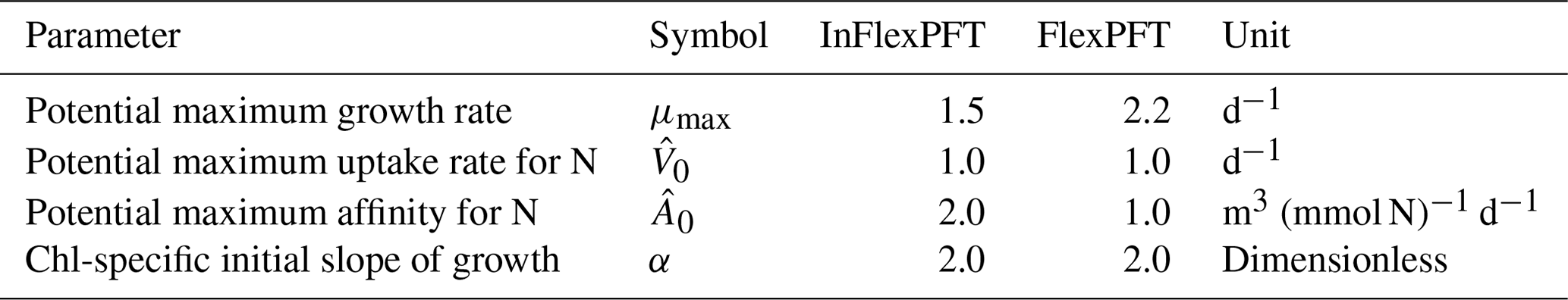
Here, we briefly describe the two phytoplankton growth rate equations, InFlexPFT and FlexPFT, used in this study, which appear in the first term of the right-hand side, μP, in Eq. (A2). In both models, the phytoplankton growth rate, μ (d−1), depends on the irradiance, I, which is the intensity of photosynthetically active radiation calculated from the daily mean short-wave radiation (W m−2) of JRA55-do, the nitrogen, N (mmol N m−3), and the temperature, T (∘C). The phytoplankton growth rate equation is expressed by multiplying the N uptake, I limitation, and T limitation. N and T are taken from the coupled physical-biological models' output. The InFlexPFT for growth rate, μIFL () (d−1), is based on the optimal uptake kinetics equation (Smith et al., 2009):
where μmax is the potential maximum growth rate (d−1), is the potential maximum uptake rate for N (d−1), and is the potential maximum affinity for N (m3 (mmol N)−1 d−1), following the optimal uptake equation (Table 1). Compared to the Monod equation for growth as a function of ambient nutrient concentration, as typically applied in fixed-composition models, this equation yields a similar response but with a slightly flatter shape (Smith et al., 2009). S(I,T) specifies the dependence on I (Pahlow et al., 2013), and F(T) is the Arrhenius-type temperature dependence. S(I,T) and F(T) are respectively defined as
Here, α is the Chl-specific initial slope of growth versus light intensity (dimensionless, Table 1), and is the Chl : C ratio (g chl (mol C)−1) of the chloroplast, as described by Pahlow et al. (2013). In the InFlexPFT, the Chl : C ratio is set to a constant value (), assuming fixed stoichiometry without photoacclimation. Ea is the activation energy (4.8×10⁴ J mol−1), which is set to a constant value corresponding to a doubling of growth rate for a 10 ∘C increase in temperature (i.e. Q10=2.0), which is a typical empirically based value for the temperature sensitivity of phytoplankton growth rates (Eppley, 1972; Bissinger et al., 2008), R is the gas constant (8.3145 J (mol K)−1), and Tref is the reference temperature (taken as 20 ∘C).
The FlexPFT assumes a photoacclimation theory based optimal resources allocation trade-off between light and nutrients (Pahlow et al., 2013; Smith et al., 2016). The growth rate, (d−1) (Smith et al., 2016), is
where Qs is the structural minimum cell quota (mol N (mol C)−1), given as a fixed parameter (, where Q0(=0.039) is the minimum cell quota, Edwards et al., 2012); Q is the nitrogen cell quota, i.e. the intracellular N content per unit carbon biomass (mol N (mol C)−1) as a function of I, N, and T; and fV is the fractional allocation of intracellular resources to nutrient uptake (dimensionless) as defined by Pahlow et al. (2013). The cell quota, , is
where is the potential nutrient uptake rate (mol N (mol C)−1 d−1), and ζN is the energetic respiratory cost of assimilating inorganic nitrogen (0.6 mol C (mol N)−1, Pahlow and Oschlies, 2013). The potential nutrient uptake rate, , is
The fractional allocation of intracellular resources to nutrient uptake, , as defined by Pahlow et al. (2013) is
The differences between the two models are the trade-off between light and nutrient acquisition (Eqs. 5, and 7) and the variable Chl : C ratio () in the light limitation term of Eq. 2, which are only included in the FlexPFT (Eq. 4) to account for the flexible response of phytoplankton growth to changing light and nutrient conditions (Eqs. 2, 5, 6, and 7). The optimal value of the Chl : C ratio in the FlexPFT is applied when the irradiance I exceeds the threshold irradiance, below which the respiratory cost outweighs the benefits of producing chlorophyll (Pahlow et al., 2013; Smith et al., 2016). The InFlexPFT has the same nutrient uptake response as the FlexPFT (Eqs. 1 and 6), and the Chl : C ratio in the light limitation term (Eq. 2) is set to a constant value. The same temperature dependence, F(T), is assumed in both models (Eq. 3). The parameter values , and α (Table 1) used in Eqs. 1 to 7 for the phytoplankton growth rate were tuned, separately for each coupled model, to confirm the reproducibility of the climatological seasonal variability of observed N and the Chl patterns in the near-surface of the North Pacific. In this study, we have chosen to apply different parameter values, based on the separate tuning of each coupled model (Table 1), in order to make a fair comparison of each model's ability to reproduce the climatological seasonal and spatial variability of N and Chl. Applying the same parameter values for both models would not be meaningful, given their different meanings within the different growth equations. For example, the potential maximum growth rate, μmax, is 1.5 (d−1) for the InFlexPFT, compared to 2.2 (d−1) for the FlexPFT. Increasing the potential maximum growth rate decreases the surface N concentration in the subpolar gyre, to the point of depleting nutrients during summer, while increasing the surface Chl concentration across the whole gyre.
Compared to the InFlexPFT, the FlexPFT model yields different growth rates because it instantaneously optimizes both the allocation factor, (Eq. 7), and the Chl : C ratio of the chloroplast, , which appears in the light limitation term, S(I,T) (Eq. 2). Therefore, it is possible to understand the modelled patterns of Chl (mg m−3) and PP (mgC m−3 d−1) over the North Pacific Ocean by comparing the models in terms of their expressions for growth rate, μ, as a function of I, N, and T. Results are presented for simulated years 2000 to 2019 with verifiable observation data. For the InFlexPFT, the Chl concentration (mg m−3) is P (mmol N m−3) × the constant Chl : N ratio (1.59 g Chl (mol N)−1), and PP (mgC m−3 d−1) is μIFLP (mmol N m−3 d−1, Eq. 1) × the fixed C : N ratio (Redfield ratio = 106 : 16 mol C (mol N)−1). In the FlexPFT, the Chl concentration (mg m−3, ) is the phytoplankton concentration P (mmol N m−3) × the variable Chl : N ratio (g Chl (mol N)−1, ), and the primary production, PP (mgC m−3 d−1), is μFLP (mmol N m−3 d−1, Eq. 4) × the variable C : N ratio (mol C (mol N)−1), ) (Eq. 5 and Smith et al., 2016).
2.3 Observational data
The average model results for the last 20 years (2000–2019) were compared with satellite data, in situ observations, and the climatological data (Chl, nitrate, and temperature) to investigate the large-scale variation over the North Pacific. Although the model and observation periods differ somewhat, using the satellite and in situ observation data observed during the simulation period (the 2000s), we compare whether the horizontal and vertical patterns of climatological seasonal variations can reproduce the patterns captured by the satellite and the snapshot observations. We focused especially on the Chl and PP patterns, which strongly reflect effects of the different assumptions about how growth rates depend on light and nutrients. Sea-surface Chl satellite imagery is derived from the Moderate Resolution Imaging Spectroradiometer (MODIS) aboard Aqua (https://oceancolor.gsfc.nasa.gov/data/10.5067/AQUA/MODIS/L3M/CHL/2022/, last access: 1 March 2022) using the seasonal climatological data (averaged from 2003 to 2019) of the level-3 global browser. Ship-observed Chl data along the two sections (north–south and east–west) in the North Pacific are available from the websites of the Japan Meteorological Agency, JMA (https://www.data.jma.go.jp, last access: 1 March 2022), and the Japan Oceanographic Data Center, JODC (https://www.jodc.go.jp, last access: 1 March 2022), respectively. Along the north–south section (165∘ E) in the western North Pacific, JMA research vessels have observed regularly from 2005 to the present. Along the east–west section (around 35∘ N) in the central North Pacific, observations were conducted in summer 2002 to 2003 and published by the JODC. Seasonal climatological nitrate and temperature distributions are acquired from the World Ocean Atlas 2018 (WOA18) (Garcia et al., 2018a; Locarnini et al., 2018). The PP data sets are available at three time-series stations: stations K2 (47∘ N, 160∘ E) and S1 (30∘ N, 145∘ E) in the western North Pacific, as implemented by the K2S1 project (Matsumoto et al., 2014, 2016; Honda et al., 2017) (https://www.jamstec.go.jp/egcr/e/oal/k2s1.html, last access: 1 March 2022), and station ALOHA (22.45∘ N, 158∘ W) in the central North Pacific, as operated under the Hawaii Ocean Time series (HOT) program (Karl et al., 1996, 2021) (https://hahana.soest.hawaii.edu/hot/, last access: 1 March 2022).
This section assesses the models' performance and examines the impact of physiological flexibility on the modelled Chl and PP by comparing the results of two coupled physical-biological (InFlexPFT and FlexPFT) models against MODIS-Aqua imagery and vertical profiles of in situ observations (JMA and JODC ship observation lines). Modelled phytoplankton is controlled by various ecological processes (e.g. grazing, mortality, export, and recycling), but in this study, we focus on the implications of specific assumptions about how the phytoplankton growth rate depends on light, nutrients, and temperature. The eddy-resolving ocean circulation model (OFES2) has fine horizontal resolution (∘, about 10 km) and reproduces the western boundary current, the Kuroshio, the observed variability in the Kuroshio Extension region between the subtropical and subpolar gyres, mesoscale eddies, and upwelling events (e.g. Masumoto et al., 2004; Sasai et al., 2010; Sasaki et al., 2020). In addition, the seasonal variability of the T and N fields in the near-surface over the North Pacific are also well reproduced (not shown). These physical processes directly or indirectly affect the nutrient and light environments and biogeochemical processes (e.g. Oschiles, 2002; Gruber et al., 2011; Levy et al., 2014; Sasai et al., 2010, 2019), and are important for supplying the nutrients needed by phytoplankton, especially in the coastal upwelling regions and the oligotrophic subtropical gyre. Here we focus on the different assumptions about how phytoplankton growth rate depends on ambient nitrogen concentration and light intensity. First, the reproducibility of the seasonal and horizontal Chl distributions is described. As the Chl concentration in the FlexPFT is calculated from , and reflects the changes in and Q, we examine how variations in C : N : Chl ratios impact the surface Chl pattern. Next, we compare the results of the two coupled physical-biological models in terms of Chl and PP along two vertical transects (north–south and east–west, respectively) in the North Pacific, and discuss the reasons for the differences, especially the role of photoacclimation in the formation of SCM and the role of the growth rate in the variable C : N : Chl ratios of phytoplankton. Finally, the difference in the PP calculated by these two models over the North Pacific and the comparison with the limited PP vertical profiles are discussed. The extent to which the different growth rates (InFlexPFT vs. FlexPFT) affect the estimated PP is described.
3.1 Comparison of surface Chl patterns
Figure 1 shows the surface Chl distributions as simulated over the North Pacific by the two models, which are compared with MODIS-Aqua imagery to assess the two models' performance. Overall, using an eddy-resolving (∘) OFES2, the two models reproduce the climatological seasonal variations of the surface Chl pattern between the subtropical (< 0.2 mg m−3, blue shaded) and subpolar (> 0.2 mg m−3, green and yellow shaded) gyres, as captured by the MODIS-Aqua imagery. In particular, the contrast between the two gyres and the coastal upwelling region is seen more clearly when using the OFES2 than lower-resolution (e.g. 1∘, about 100 km) models (e.g. Moore et al., 2001; Vichi et al., 2007; Follows et al., 2007; Göthlich and Oschlies, 2012). In addition, both models reproduce the boundary (0.2 mg m−3) between the subtropical and subpolar gyres, its seasonal variations, and the high concentrations (> 0.4 mg m−3) in the coastal upwelling regions (California coast) seen in the MODIS-Aqua imagery. Compared to the InFlexPFT, the FlexPFT model produces greater variations and steeper horizontal gradients of Chl concentration. Especially in the open ocean north of 30∘ N, coastal upwelling regions off the western coast of North America, the Sea of Okhotsk, and the Bering Sea, the FlexPFT produces higher surface Chl (> 0.4 mg m−3) than the InFlexPFT, but it underestimates Chl in the subtropical gyre (south of 30∘ N, < 0.1 mg m−3). The FlexPFT also reproduces greater seasonal variation of surface Chl in the subpolar gyre, similar to the pattern in the MODIS-Aqua imagery. On the other hand, in the subtropical gyre, the InFlexPFT is more similar to the MODIS-Aqua imagery. These differences in the spatial and seasonal distributions of surface Chl result from the different phytoplankton growth rate equations (Eqs. 1 and 4). The Chl : N ratio is calculated from (photoacclimation) and Q (nitrogen cell quota, Eq. 5), and the models differ in that the FlexPFT has a variable Chl : N ratio (0.1–3.0) whereas the InFlexPFT has a fixed Chl : N ratio of 1.59. In the subtropical gyre, the FlexPFT’s Chl : N ratio is low (< 0.6), and the Chl concentration is underestimated compared with the MODIS-Aqua imagery. In the subpolar gyre and coastal upwelling regions, the FlexPFT's Chl : N ratio is high (> 1.0), and the Chl concentration is close to that in the MODIS-Aqua imagery.
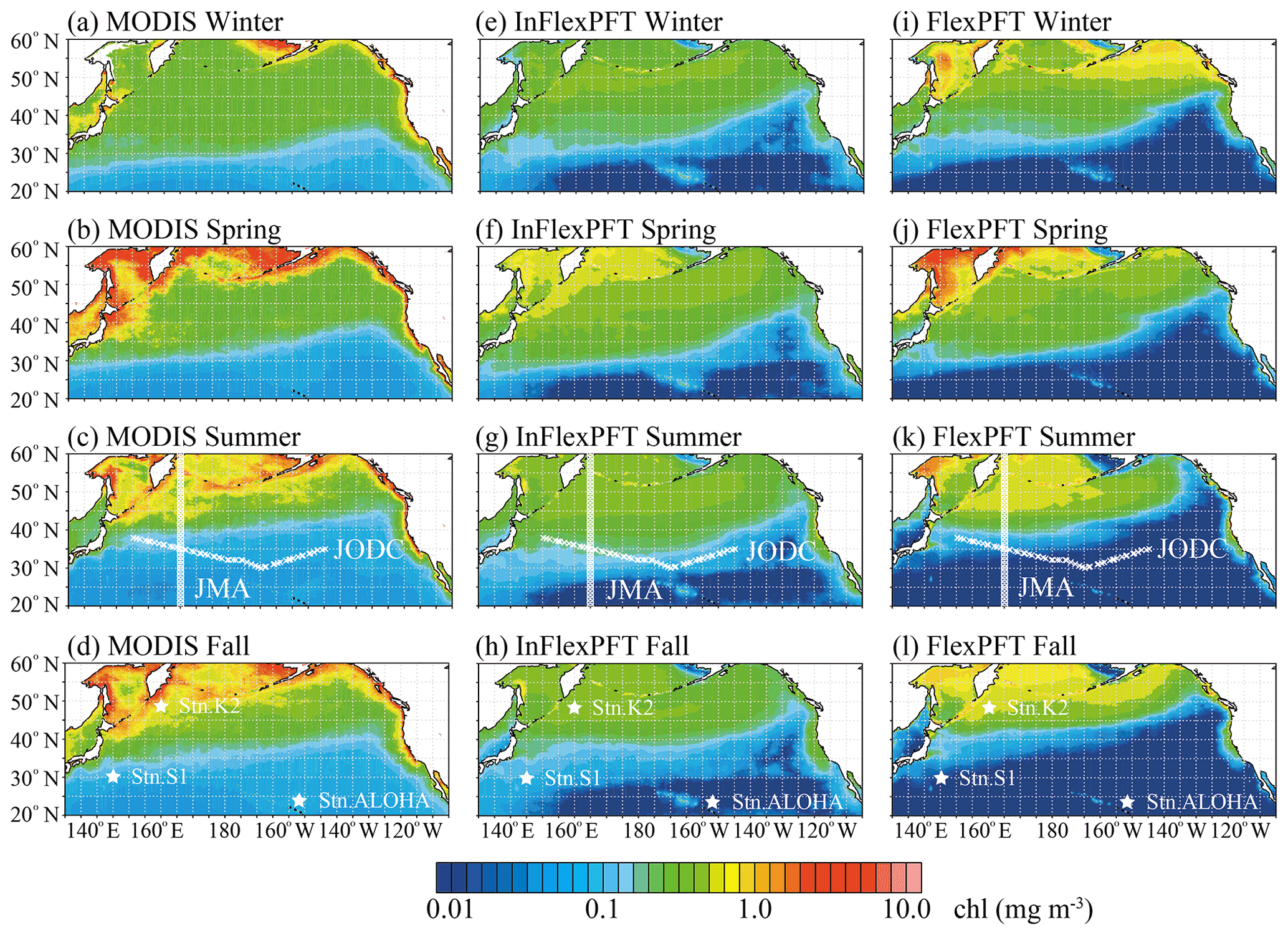
Figure 1Climatological seasonal variations of surface Chl concentration (mg m−3) from (a)–(d) MODIS-Aqua imagery and (e)–(i) two models. MODIS-Aqua imagery is averaged from 2003 to 2019 for each season. The results from each model are the season average for the period 2000–2019 for the 20 m layer closest to the surface. White circles and crosses in (c), (g), and (k) show two observation lines (the circles are the locations of the JMA data and the crosses are the locations of the JODC data). The three stars in (d), (h), and (l) show the stations that provide observed time series (station K2, station S1, and station ALOHA).
3.2 Comparison of vertical distributions of Chl and PP along the two transect lines
The limited data available from observations made by research vessels do capture key spatial and temporal distributions. Here, the reproducibility of the vertical distribution of Chl along two observation lines over the North Pacific Ocean – a north–south section along 165∘ E shown in Fig. 2, and an east-west section around 35∘ N shown in Fig. 3 – is discussed for each model. In particular, we focus on the SCM formed in summer, and discuss the effects of different assumptions about how the phytoplankton growth rate (Eqs. 1 and 4) depends on N concentration and light intensity, I, as well as their effects in combination with the temperature, T (Figs. 4, 5, 6, and 7).
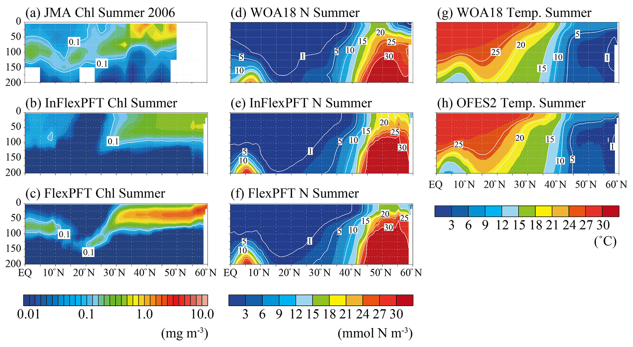
Figure 2Comparison of the vertical distributions of (a)–(c) summer (June, July and August) Chl concentration (mg m−3), (d)–(f) summer N concentration (mmol N m−3), and (g)–(h) summer T (∘C) along 165∘ E (north–south section; white circles in Fig. 1). Panel (a) shows in situ observation data from the summer of 2006 taken by the JMA research vessel. Panels (d) and (g) show data for the climatological summer from WOA18. Panels (b), (c), (e), (f), and (h) show the models' average values for the summer during the 2000–2019 period. The white area in (a) represents missing data.
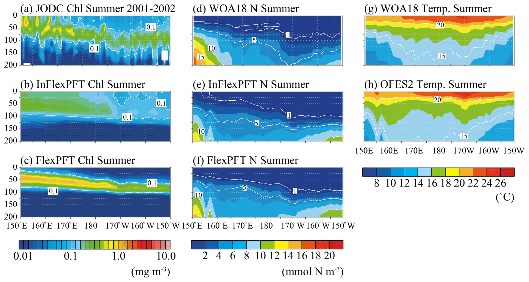
Figure 3Comparison of the vertical distributions of (a)–(c) summer (June, July and August) Chl concentration (mg m−3), (d)–(f) summer N concentration (mmol N m−3), and (g)–(h) summer T (∘C) along the location of the white crosses (east–west section) in Fig. 1. Panel (a) shows in situ observation data collected by the JODC in the summer in 2001–2002. Panels (d) and (g) show data for the climatological summer from WOA18. (b), (c), (e), (f), and (h) show the models' average values for the summer during the 2000–2019 period. The white area in (a) represents missing data.
JMA research vessels have made observations on the north–south line along 165∘ E regularly since 1997, with good seasonal coverage. The best data coverage for vertical Chl profiles is available for the summer of 2006. The observed SCM (> 0.1 mg m−3) depth varies from 50 m near the Equator to 150 m in subtropical regions, and the FlexPFT clearly reproduces the observed pattern of SCM near the nutricline (close to 1 mmol N m−3) along the 165∘ E line (Fig. 2), with simulated values close to the observed SCM (Fig. 2a and c). However, the FlexPFT underestimates near-surface Chl (< 0.02 mg m−3, dark blue shaded). By contrast, the InFlexPFT (Fig. 2b) cannot reproduce the observed SCM, even though its modelled distributions of N and T are similar to the corresponding observations (Fig. 2d, e, f, g, and h). The N and T distributions reproduced in the OFES2 are mainly controlled by the physical processes, and the difference in vertical Chl distributions is influenced by the difference in the response of the phytoplankton growth to the light and nutrient conditions (Eqs. 1 and 4). The FlexPFT, which incorporates the photoacclimation and the trade-off between light and nutrient acquisition, reproduces the observed vertical Chl distributions much better than the InFlexPFT, especially the depth and structure of SCM.
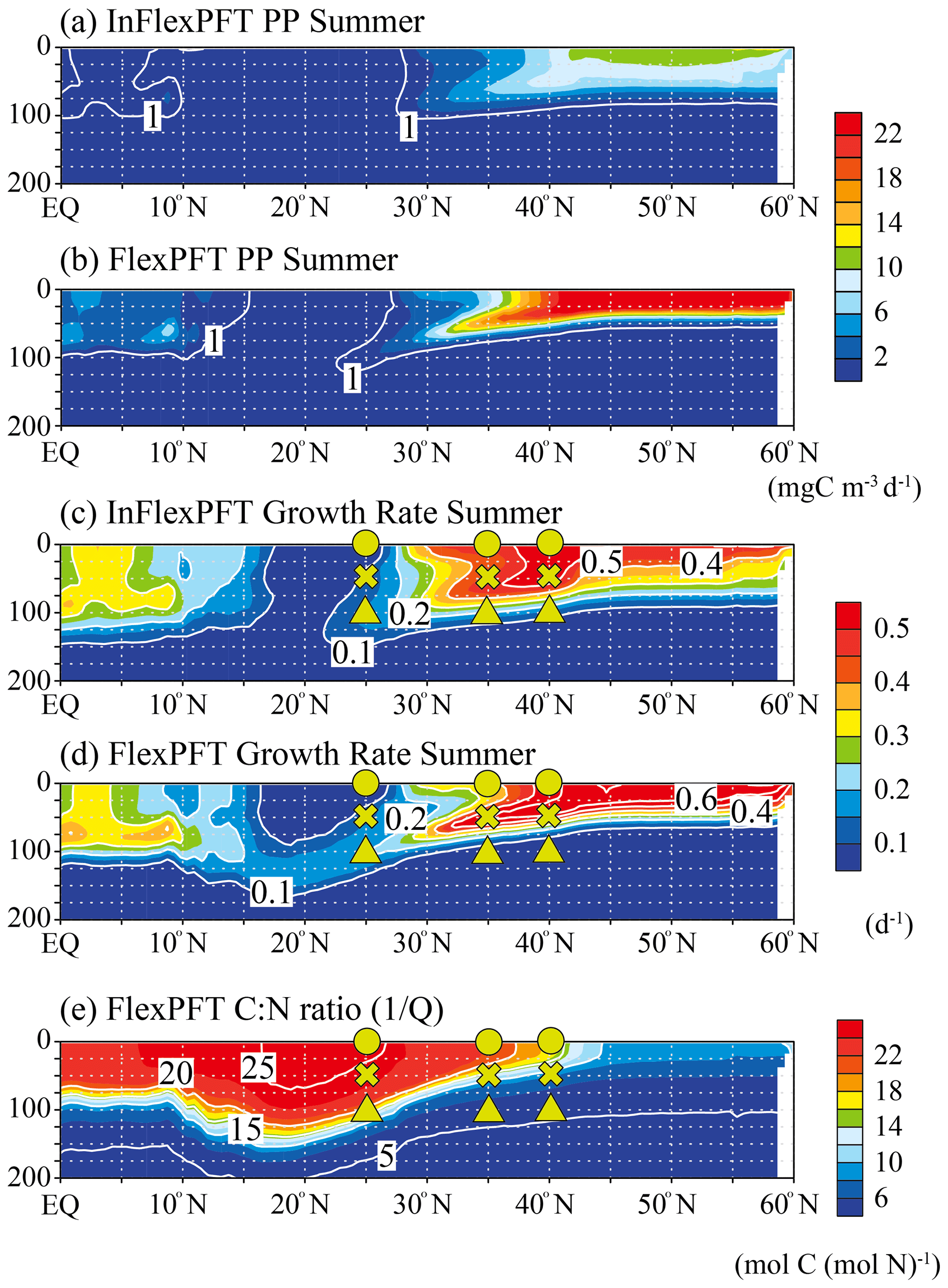
Figure 4Comparison of the vertical distributions of (a)–(b) summer primary production (mg C m−3 d−1) and (c)–(d) summer phytoplankton growth rate (d−1) between the two models, and (e) the vertical distribution of the summer C : N ratio in the FlexPFT along 165∘ E (north–south section; shown by white circles in in Fig. 1). These figures show the average values for the summer during the 2000–2019 period.
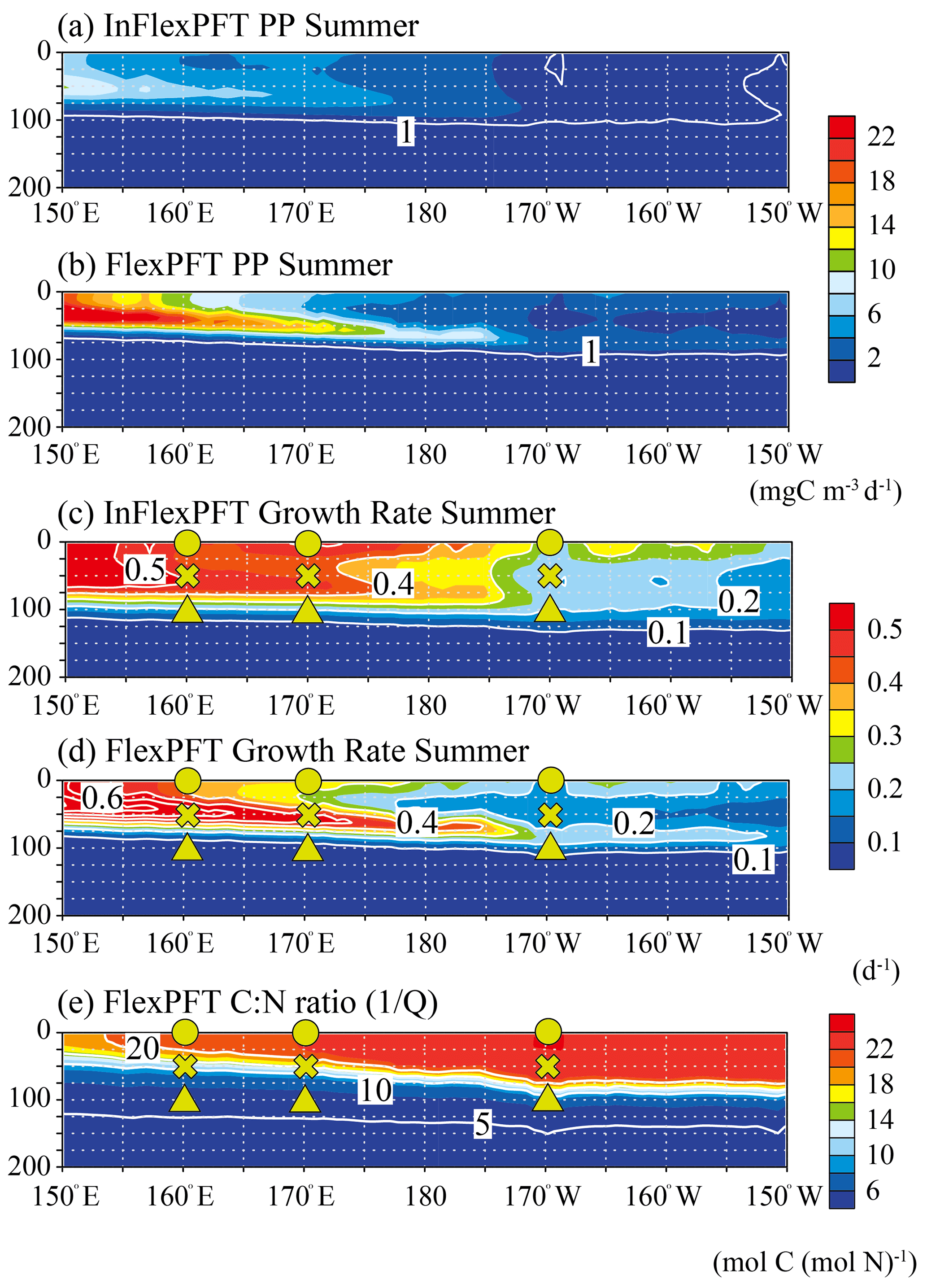
Figure 5Comparison of the vertical distributions of (a)–(b) summer primary production (mg C m−3 d−1) and (c)–(d) summer phytoplankton growth rate (d−1) between the two models, and (e) the vertical distribution of summer C : N ratio in the FlexPFT, along the location of white crosses (east–west section) in Fig. 1. These figures show the average values for the summer during the 2000–2019 period.
The vertical distribution of Chl also varies with longitude along the east–west transect around the boundary (35∘ N) between the subpolar and subtropical gyres (Fig. 3). The limited JODC Chl observations (summer 2001–2002) span the east and west of the North Pacific. The observed SCM (> 0.1 mg m−3) appear between 50 and 150 m depth and deepens to the east (Fig. 3a), following the distribution of nutricline depths (close to 1 mmol N m−3) (Fig. 3d). Compared to the north–south transect, here the near-surface T gradient is not as steep (Figs. 2 and 3), with T near the surface decreasing from the centre to the east and west (Fig. 3g). The model reproduces the observed T distribution, and the modelled N distribution is similar to the observed data (Fig. 3e, f, and h). The FlexPFT clearly reproduces the observed SCM around the nutricline depth (Fig. 3c and f) from east to west, whereas the InFlex does not (Fig. 3b). On the eastern side of the North Pacific, both models have a deep nutricline depth, and the FlexPFT underestimates the observed Chl (Fig. 3a and c) and N (Fig. 3d and f).
To clarify the mechanistic reasons for differences in the vertical distributions of Chl between the two models (Figs. 2 and 3), the vertical distributions of the models' PP (mgC m−3 d−1), the related phytoplankton growth rate (d−1) from Eqs. (1) and (4), and the variable C : N ratio (the reciprocal of the N to C ratio of phytoplankton, , Eq. 5) in the FlexPFT are shown in Figs. 4 and 5. The PP was calculated from the phytoplankton growth rate and the C : N ratio, which is variable for the FlexPFT (Figs. 4e and 5e), whereas it is constant for the InFlexPFT. In summer (Figs. 2 and 3), the SCM are clearly formed in the subsurface layer, except for the subpolar gyre (north of 40∘ N). The vertical distributions of the PP and phytoplankton growth rate form maxima along the nutricline depth. Both models predict high PP (> 10 mgC m−3 d−1) near the surface in the subpolar regions along 165∘ E, along with minimal PP (< 1 mgC m−3 d−1) near the bottom of the euphotic layer, which is close to 100 m depth (Fig. 4a and b). Overall, compared to the InFlexPFT, the FlexPFT produces greater PP, with profiles extending deeper into the subsurface (100 m depth) to the south of 30∘ N. Both models produce fast growth rates in the subpolar surface layers (> 0.5 d−1) and the subtropical subsurface layers (> 0.2 d−1) (Fig. 4c and d). Especially in the subtropical subsurface layers, the FlexPFT predicts much faster growth than the InFlexPFT, and this difference in phytoplankton growth rate is reflected in the vertical distributions of Chl (Fig. 2b and c) and PP (Fig. 4a and b). The variable C : N ratio in the FlexPFT (Fig. 4e) also contributes substantially to its greater PP values (Fig. 4d) compared to the constant C : N ratio in the InFlexPFT (Fig. 4c). In Fig. 4e, the C : N ratio in the FlexPFT is high (> 20) near the surface around the Equator and subtropical regions, and near the Redfield ratio (106 : 16 = 6.625) elsewhere in the subpolar region and below the euphotic layer (below 100 m depth). Our results show that, compared to the assumption of constant C : N : Chl ratios, as done in the InFlexPFT, accounting explicitly for variable C : N ratios (4.0 to 25.0 in Fig. 4e) and the acclimated growth response of phytoplankton, as done in the FlexPFT, yields substantially better reproduction of the Chl and PP profiles within the euphotic layer.
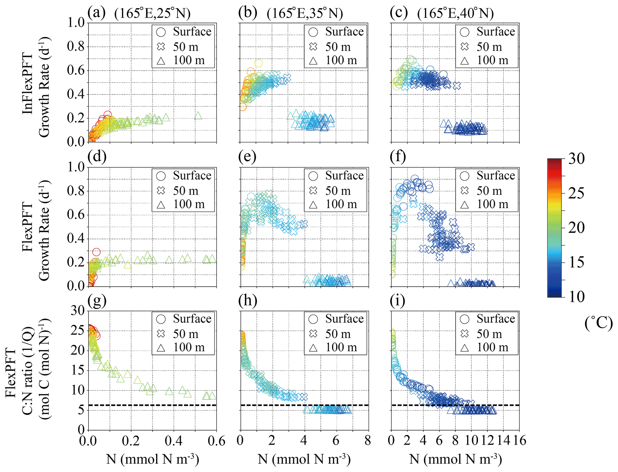
Figure 6(a)–(f) Monthly mean phytoplankton growth rate (d−1) in summer in 2000–2019 from Fig. 4c and d versus summer monthly mean N concentration (mmol N m−3) from Fig. 2e and f for each depth (circles: surface, crosses: 50 m depth, triangles: 100 m depth in Fig. 4c and d) and each model, and (g)–(i) summer monthly mean C : N ratio versus summer monthly mean N concentration in the FlexPFT model. The colour in each figure represents the summer monthly mean T (∘C) in Fig. 2h. Dashed lines in (g), (h), and (i) represent a constant C : N (106 : 16 = 6.625) ratio value.
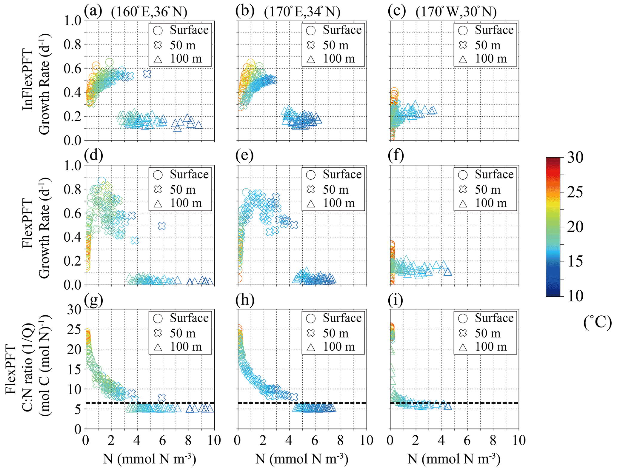
Figure 7(a)–(f) Monthly mean growth rate (d−1) in summer in 2000–2019 from Fig. 5c and d versus summer monthly mean N concentration (mmol N m−3) from Fig. 3e and f for each depth (circles: surface, crosses: 50 m depth, triangles: 100 m depth in Fig. 5c and d) and each model, and (g)–(i) summer monthly mean C : N ratio versus summer monthly mean N concentration in the FlexPFT model. The colour in each figure represents the summer monthly mean T (∘C) in Fig. 3h. Dashed lines in (g), (h), and (i) represent a constant C : N (106 : 16 = 6.625) ratio value.
As in Fig. 4, the vertical distributions of modelled PP (mgC m−3), the related phytoplankton growth rate (d−1) from Eqs. (1) and (4), and the variable C : N ratio in the FlexPFT (Eq. 5) are shown in Fig. 5, but for the east–west section. Both models predict high PP (> 8 mgC m−3 d−1) between 50 and 100 m, with shallower distributions on the west side and deeper ones toward the east (Fig. 5a and b). Compared to the InFlexPFT, the FlexPFT predicts higher PP (> 10 mgC m−3 d−1), especially in the subsurface (near 50 m depth). Although both models predict faster growth on the west side (> 0.5 d−1), decreasing towards the east (< 0.2 d−1), their patterns differ (Fig. 5c and d). In the InFlexPFT, the phytoplankton growth rate is fastest near the surface and decreases with depth. On the other hand, the FlexPFT predicts increasing growth rate with depth from the surface to intermediate depths. Both models produce subsurface maxima in PP (Fig. 5a and b), with a stronger pattern for the FlexPFT model. The FlexPFT predicts an even stronger subsurface maximum in the vertical distribution of Chl (Fig. 3c). This results from the FlexPFT's combination of photoacclimation and variable C : N ratio, which is consistently high (> 10) in the euphotic layer (0–100 m) (Fig. 5e). Below the euphotic layer and to the west side, the FlexPFT's C : N ratio approaches the Redfield ratio (106 : 16 = 6.625), and therefore the modelled Chl and PP differ less between the two models.
To examine the interdependent impacts of N concentration and light intensity, I, on the phytoplankton growth rate in the FlexPFT, as compared with their simple multiplicative dependencies in the InFlexPFT, Figs. 6 and 7 show scatter diagrams of modelled phytoplankton growth rate and variable C : N ratio () versus N concentration (mmol N m−3) at the three locations indicated along 165∘ E in Fig. 4 and around 35∘ N in Fig. 5. The different depths (0, 50, and 100 m) correspond to different light intensities at each location (strong at the surface and weaker at 100 m depth). Compared to the InFlexPFT, the FlexPFT maintains faster growth, as either light or nutrients become limiting everywhere. The phytoplankton growth rate equations (Eqs. 1 and 4) also depend on the temperature, T (Eq. 3), as shown by the colours. The explicitly formulated temperature dependence of the growth rate is the same in both models. In general, I and T both depend on latitude, and both decrease with increasing depth. At 25∘ N latitude (Fig. 6a and d), in the subtropical gyre, both models predict phytoplankton growth rates exceeding 0.2 (d−1) near the surface, despite the low N concentrations (< 0.1 mmol N m−3), as high I and T enhance the growth rate. Compared to the InFlexPFT, the FlexPFT maintains faster growth rates at the surface and 50 m because it dynamically allocates intracellular resources to cope with variations in N concentration and I (Smith et al., 2016, and Eq. 4). At the boundary between the subtropical and subpolar gyres, which lies approximately between 35 and 40∘ N latitude, the two models predict clearly different patterns of phytoplankton growth rate compared to those at 25∘ N (Fig. 6b, c, e, and f). At the gyre boundary and in the subarctic, both models tend to produce faster growth rates at 50 m, where the availability of light and nutrients is better balanced to support phytoplankton growth, compared to the surface and 100 m depth. Compared to temperature, nutrient and light limitation exert greater control over the modelled growth rates with both models, but more so for the FlexPFT. Nutrient limitation is the strongest determinant of growth rates at the surface and intermediate (50 m) depth, whereas light limitation strongly suppresses growth rates (and their range of variability) at 100 m depth.
Similar to Fig. 6, Fig. 7 shows modelled phytoplankton growth rates at three selected locations along the 35∘ N latitude transect (Fig. 5). The two locations (160∘ E, 36∘ N, and 170∘ E, 34∘ N) on the west side of the North Pacific are close to (165∘ E, 35∘ N) in Fig. 6, and have similar characteristics. At these locations, near the boundary of the subtropical and subpolar gyres, the nutricline depth is shallower than on the eastern side. The InFlexPFT at the surface and 50 m depth shows two curves of phytoplankton growth rate versus N concentration, I, and T (Fig. 7a and b), similar to Fig. 6b. Again, the InFlexPFT predicts the fastest growth rates at the high T (> 20∘C), despite low N concentrations. On the other hand, the FlexPFT's growth rates are more clearly related to the ambient N concentration and have a less apparent relationship to T, despite assuming the same T dependence in both models (Fig. 7d and e). As in Fig. 6, compared to the InFlexPFT, the FlexPFT predicts faster phytoplankton growth rates, with maximal growth at intermediate N concentrations (despite the lower T compared to the surface), and a wider variation of growth rate. At the eastern-most location (170∘W, 30∘ N), as shown in the right-most column of Fig. 7c and f, the patterns are more similar to those for the subtropical area shown in the left-most column of Fig. 6a and d, albeit with somewhat greater variability of growth rate for both models near the surface, where temperatures are high and nutrients scarce. Just as at the subtropical location (25∘ N latitude) shown in the left-most column of Fig. 6, the InFlexPFT also exhibits a stronger apparent temperature sensitivity (and hence a wider range of growth rates) than the FlexPFT at this location, but only near the surface here. Neither model shows a strong apparent relationship between growth rate and N concentration at this location, indicating that light, nutrients, and temperature all substantially limit the growth here.
Compared to the InFlexPFT, the FlexPFT produces higher PP because its variable C : N ratio (4.0 to 25.0) substantially exceeds the Redfield ratio (106 : 16 = 6.625), with a consistent increase in C : N ratio from intermediate depths to the surface obtained everywhere (Figs. 6 and 7). At 35 and 40∘ N, where the phytoplankton growth rate reaches its maximal values, the C : N ratios are between 10 and 15 (Figs. 6h, i, 7g, and h), which enhances PP (Figs. 4b and 5b). Along the east–west transect as well (Fig. 7), the FlexPFT again predicts maximal C : N ratios near the surface (> 20), where nutrient concentrations are lowest and light (and temperature) levels are highest, with a similar range of C : N ratios to that obtained along the north–south transect (Fig. 6). On the west side, the C : N ratio in the FlexPFT (Fig. 7g and h) exceeds the Redfield ratio (> 6.625) except below the euphotic layer, and growth rates are maximal at intermediate nutrient concentrations and light intensities. On the other hand, on the east side, where ambient nutrient concentrations are consistently low despite the high C : N ratio in the FlexPFT (> 20 in Fig. 7i), modelled growth rates differ little between the two models.
Overall, at the surface and 50 m depth, the modelled patterns of growth rate versus N concentration are more clearly separated with the FlexPFT model, which produces a steeper and more consistent increase in growth rate from low to intermediate N concentrations compared to the InFlexPFT. These variations in the locally realized maximum growth rate result from the FlexPFT's growth optimization scheme, which re-allocates intracellular resources, resulting in an interdependent response to I and N availability (Fig. 3 of Smith et al., 2016, and Eq. 4). By contrast, the InFlexPFT’s simple multiplicative dependencies on I and N concentration result in a steeper decrease in growth rate as either resource becomes limiting. Despite the assumption of the same inherent T sensitivity in both models, the optimal resource allocation thus results in a weaker apparent relationship between modelled growth rates and ambient T in the FlexPFT model, which predicts the fastest growth rates at intermediate N concentrations despite the lower T than at the surface. By contrast, the InFlexPFT model, because of its weaker dependence on nutrient concentration and light, predicts the fastest growth rates at the highest temperatures, along with a stronger apparent relationship between growth rate and ambient temperature.
3.3 Vertical profiles of PP at three stations and PP patterns
Figure 8 shows a direct comparison of the modelled daily mean and observed vertical profiles of PP for three time-series stations in the North Pacific: station K2 in the western subpolar gyre and stations S1 and ALOHA in the western and eastern subtropical gyres, respectively. At station K2, observed PP is more variable above 25 m depth and less variable below 25 m depth (Fig. 8a). Overall, compared to the FlexPFT (8 to 50 mg C m−3 d−1), the InFlexPFT predicts less temporal variability of PP (5 to 15 mg C m−3 d−1), except below 50 m depth at station K2, where the FlexPFT predicts faster growth than the InFlexPFT (Fig. 4c and d). At station S1, the temporal variation of observed PP is greater above 50 m depth, with less variability below 50 m depth (Fig. 8b). Compared to station K2 (subpolar gyre), the highest PP occurs deeper at station S1 (subtropical gyre), where light limitation is more substantial, which suggests that PP could be enhanced by an increase in light levels, despite the relatively low N concentrations. Compared to the InFlexPFT (1 to 8 mg C m−3 d−1), the FlexPFT shows greater temporal variation of PP above 75 m depth (3 to 50 mg C m−3 d−1). This difference depends on whether the phytoplankton growth ratio calculated by the model reflects the optimal N and light environment (FlexPFT) or not (InFlexPFT). Unlike the two stations in the western North Pacific, at station ALOHA, both models underestimate the observed PP (Fig. 8c). The observed PP from the surface to 100 m depth is large, and the PP near the surface is about the same as at the western station S1. The FlexPFT underestimates the mean PP (2 mg C m−3 d−1), but the temporal variation (1 to 10 mg C m−3 d−1) is closer to the observed variability than that obtained with the InFlexPFT (< 1 mg C m−3 d−1). Overall, compared to the InFlexPFT, the FlexPFT agrees better with the observed vertical PP profiles and their temporal variability.

Figure 8Comparison of vertical primary production (mg C m−3 d−1) between observed station data and data from the two models at (a) station K2 (47∘ N, 160∘ E), (b) station S1 (30∘ N, 145∘ E), and (c) station ALOHA (22.45∘ N, 158∘ W) in Fig. 1. The observed data (crosses) are from 2010–2019 for station K2, 2010–2013 for station S1, and 2000–2019 for station ALOHA. The mean (solid line), maximum (dashed line), and minimum (dotted line) primary production in 2000–2019 are shown for the two models. Blue lines are for InFlexPFT and red lines are for FlexPFT. The stations are shown as three stars in Fig. 1.
The vertical distribution of PP differs along the two transect lines (north–south and east–west, respectively) (Figs. 4 and 5). To investigate the models' PP variations within the euphotic layer, Fig. 9 shows the seasonal variations of vertically integrated PP from the surface to 100 m depth for the two models. The InFlexPFT produces weak seasonality for PP (Fig. 9a, b, c, and d), with maximal values in spring (> 800 mg C m−2 d−1) at the boundary between the subtropical and subpolar gyres (Fig.9b), because the spring bloom occurs both horizontally and vertically (e.g. Fig. 1f). At the gyre boundary, in addition to the surface, primary production is greater compared to other regions. In this region, the nutricline depth (close to the base of the euphotic layer) and the light intensity are optimal for spring production. Along the east–west transect, from 30 to 40∘ N, PP varies with N concentration, which is high on the west side and low on the east side (Fig. 3d, e, and f). In summer and fall, when the N concentration in the subtropical gyre decreases in the euphotic layer, even where the light intensity, I, is sufficient, N availability limits the phytoplankton growth rate (Eq. 1), so that PP (< 400 mg C m−2 d−1) does not increase (Fig. 9c and d). On the other hand, in the subpolar gyre, PP (> 400 mg C m−2 d−1) increases with N in winter, summer, and fall (Fig. 9a, c, and d). In the coastal upwelling regions, N supplied from below the euphotic layer sustains a higher PP (> 800 mg C m−2 d−1) compared to the open ocean. The FlexPFT predicts wider seasonal variations of PP across the North Pacific (Fig. 9e, f, g, and h), which are especially noticeable at the boundary between the subtropical and subpolar gyres, along the Kuroshio Current flowing south of Japan, and in the coastal upwelling region off California. Compared with the seasonal variations of PP in the InFlexPFT, the FlexPFT's growth rate and the variable C : N ratio have a great influence on the spatiotemporal variations of PP (Figs. 4, 5, and 8). The FlexPFT's springtime PP reaches twice (> 1600 mg C m−2 d−1) that of the InFlexPFT (Fig. 9b and f). In the subtropical gyre, where the light intensity in the euphotic layer is sufficient for phytoplankton growth (Eq. 4), the N concentration in winter is higher than in summer and fall, and as a result, PP values are relatively high (> 800 mg C m−2 d−1), although still lower than during spring (Fig. 9e). In the subpolar gyre, where N concentrations are high, PP increases (> 1000 mg C m−2 d−1) within the euphotic layer as the light environment improves from winter to summer (Fig. 9g and h). In the coastal upwelling regions and the Kuroshio Extension, the FlexPFT, because of its optimal resource allocation, predicts much greater PP (> 1600 mg C m−2 d−1) than the InFlexPFT.
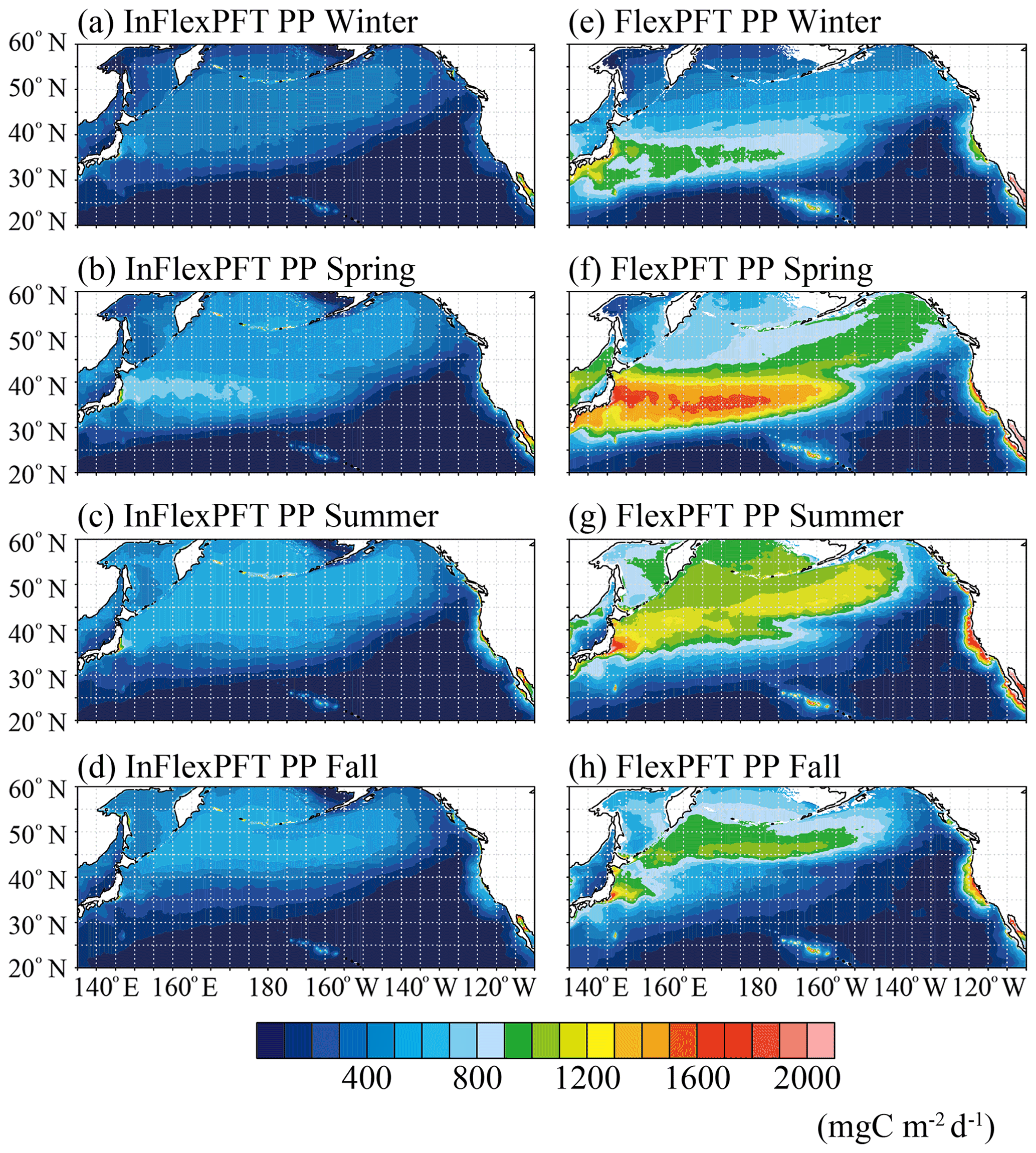
Figure 9Climatological seasonal variations of primary production vertically integrated from the surface to 100 m depth (mg C m−3 d−1) from (a)–(d) the InFlexPFT and (e)–(h) the FlexPFT. The two models are averaged from 2000 to 2019 for each season.
The difference in phytoplankton growth rate between the two models is also reflected in the spatiotemporal distribution of PP (Figs. 8 and 9), similar to the Chl distribution (Figs. 1, 2, and 3). These differences are greatest in the boundary region between the subpolar and subtropical gyres, the subpolar gyre, and the coastal upwelling region. Compared to the observed time series stations, the FlexPFT reproduces greater temporal variations than the InFlexPFT, which is more consistent with the observed variability. These results indicate that the FlexPFT (which incorporates photoacclimation and variable C : N : Chl ratios) better captures seasonal changes within the euphotic layer and near the nutricline than the InFlexPFT. From Fig. 9, the estimated primary production in the North Pacific basin (20–60∘ N, 130∘ E–110∘ W) with the FlexPFT is 5.0–5.6 PgC yr−1 and that with the InFlexPFT is 2.3–2.5 PgC yr−1 over the simulated period of 2000–2019, so the FlexPFT's estimate is about twice that of the InFlexPFT. Although not directly comparable to our estimates, the global primary production as estimated by the satellite and global biogeochemical models remains large: 38.8–42.1 PgC yr−1 over the period of 1998–2018 (Kulk et al., 2020) and 38–79 PgC yr−1 (Carr et al., 2006).
These spatial and seasonal differences in modelled chlorophyll and primary production patterns result from the different underlying assumptions about how phytoplankton respond to changing conditions. As found in previous studies (Anugerahanti et al., 2021; Kerimoglu et al., 2021; Masuda et al., 2021), our results show that photoacclimation and variable C : N : Chl ratios, as represented by the FlexPFT, are important for capturing observed distributions of PP and, especially, the SCM. Capturing the unimodal distribution of Chl : C ratio with depth is particularly important for reproducing the latter (Chen and Smith, 2018; Kerimoglu et al., 2021).
As a characteristic vertical profile, the SCM vary seasonally and across ocean regions (Cullen, 1982), driven by different light attenuation levels and nutricline depths. Various mechanisms are known and purported to contribute to SCM formation, as reviewed by Cullen (2015). These mechanisms include variations in phytoplankton growth rate along the vertical gradients of light and nutrient availability, physiologically controlled behaviours such as swimming or buoyancy regulation, and photoacclimation of pigment content. It is impossible to capture the vertical profiles of Chl with satellite observations, and it is therefore important to verify the SCM field reproduced by the model using in situ observations (e.g. Shulenberger and Reid, 1981; Furuya, 1990). Using a 3-D biogeochemical ocean model coupled with the same FlexPFT model, Masuda et al. (2021) showed that the observed global-scale SCM distribution can be reproduced by incorporating photoacclimation in response to varying nutrient and light conditions. Various mechanisms likely contribute differently in different oceanic regimes, and other mechanisms are important for reproducing specific features of SCM (e.g. Moeller et al., 2019; Wirtz and Smith, 2020). Moeller et al. (2019) proposed a new mechanism for SCM formation: light-dependent grazing by microzooplankton reduces phytoplankton biomass near the surface but allows accumulation at depth. Furthermore, vertical migration by phytoplankton can explain the occurrence of SCM consistently above the nutricline depth, which photoacclimation alone cannot (Wirtz and Smith, 2020). Wirtz et al. (2022) also suggested that phytoplankton vertical migration fuels up to 40 % (> 28 tg yr−1 N) of new production and directly contributes 25 % of the total oceanic net primary production, which their modelling study estimated at 56 PgC yr−1.
Observed elemental ratios of phytoplankton and particulate organic matter in surface layers deviate substantially from the Redfield ratio (e.g. Goldman et al., 1979; Garcia et al., 2018b; Liefer et al., 2019). Molar C : N ratios of phytoplankton vary from 4 to 60 (mol C : mol N) between phylogenetic groups. However, our current implementation of the FlexPFT model includes only one phytoplankton type, which varies its C : N ratio as it acclimates to the varying light, nutrient, and temperature levels. Sauterey and Ward (2022) found that nitrogen and temperature mostly determined variations in the C : N ratio of phytoplankton, with variable contributions from other factors across the North Atlantic. By contrast, upon applying the FlexPFT model to the North Pacific, we find that nitrogen and light levels are the primary determinants of C : N : Chl ratios, with temperature playing a lesser role. Accurate modelling of Chl and PP patterns requires that these dependencies are accounted for in order to resolve the variable elemental composition and pigment content of phytoplankton. This may be important with respect to food quality effects (e.g. Kwiatkowski et al., 2018; Matsumoto et al., 2020). That is, variations in the C : N ratio of phytoplankton are likely to impact trophic transfer and production by higher trophic levels. Although we do not address this here, it could make a good suggestion for future work.
We have focused on different formulations for the phytoplankton growth response as represented in the biogeochemical models, and investigated the acclimation of phytoplankton growth to changing light, nutrient, and temperature conditions over the North Pacific using two physical-biological models. We compared modelled Chl and primary production from a recently developed phytoplankton model, FlexPFT (Smith et al., 2016), which incorporates photoacclimation and variable C : N : Chl ratios for changing light and nutrient conditions, to those from the InFlexPFT, which lacks photoacclimation and assumes constant C : N : Chl ratios (fixed stoichiometry). Our comparison of model results against summertime observations from the North Pacific revealed that, compared to the InFlexPFT, the incorporation of photoacclimation and variable C : N : Chl ratios for changing light, nutrient, and temperature conditions in the FlexPFT yields improved reproduction of observed Chl and primary production distributions in the near-surface ocean. The assumption of instantaneous acclimation (IA) allowed computationally efficient modelling of flexible phytoplankton composition and growth response in our basin-scale model, and IA is likely to be of even greater benefit for global-scale biogeochemical models. In the future, we plan to assess model performance for other seasons, years, and decadal variations, and to apply this approach in a global ocean biogeochemical model in order to examine the response of Chl and primary production to climate change. In addition, we will proceed with research on introducing flexible physiology to the growth of multiple phytoplankton, associated food quality effects on predation by zooplankton, and the uncertainty of other biological processes, such as nitrification, grazing, mortality, export, and recycling.
The NPZD model in the OFES2 is defined as nitrogen, N, phytoplankton, P, zooplankton, Z, and detritus, D, based on Sasai et al. (2006, 2010, 2016). The evolution of the biological tracer concentration, Bi, is governed by an advective–diffusive–reactive equation:
where u is the velocity vector of OFES2, Kh is the lateral diffusion coefficient and Kz is the vertical diffusion coefficient in the OFES2, and sms(Bi) is the source-minus-sink (sms) term due to the biological activity rate (mmol N m−3 d−1) in the NPZD model. For the individual tracers (P, Z, D, and N), the sms terms are given by
where the five terms on the right-hand side of the equation for sms(P) are the phytoplankton growth rate, μ (which is or , see Sect. 2.2), the respiration of P (rP is the respiration rate for P, 0.12 d−1), the mortality of P (δP is the mortality rate for P, 0.24 d−1), the extracellular excretion of P (λ is the extracellular excretion rate of P, 0.135, no dim. (no dimension)), and the grazing of P by Z (G(P) is the grazing rate equation of Sasai et al., 2016).
where GRmax is the maximum grazing rate (1.4 d−1), λP is the zooplankton Ivlev constant (1.4 mmol N m−3), and P2Z is the zooplankton threshold value for grazing (0.04 mmol N m−3). In this study, we adopt two different formulations of phytoplankton growth (InFlexPFT and FlexPFT, see Sect. 2.2), μ, in the first term on the right-hand side of Eq. (A2). The four terms of the equation for sms(Z) are the grazing of P by Z, the excretion of Z (γ1 is the assimilation efficiency of Z (0.7, dimensionless) and γ2 is the growth efficiency of Z (0.3, dimensionless)), the egestion of Z, and the mortality of Z (δZ is the mortality rate for Z, 0.12 d−1). The six terms of the equation for sms(D) are the mortality of P, the egestion of Z, the mortality of Z, the decomposition from D to N (δD is the decomposition rate from D to N, 0.3 d−1), and the sinking of D (Ws is the sinking velocity, which is 30 m d−1 in the upper 1000 m and 300 m d−1 below 1000 m). The five terms of the equation for sms(N) are the phytoplankton growth, the respiration of P, the extracellular excretion of P, the excretion of Z, and the decomposition from D to N. More details about the biological parameters are described in Sasai et al. (2006), Sasai et al. (2010), and Sasai et al. (2016).
The OFES2-coupled NPZD model simulations are available upon request. Observed data used in this study are available at the following sites: the surface Chl satellite imagery of MODIS-Aqua data is available for download at https://oceancolor.gsfc.nasa.gov/data/10.5067/AQUA/MODIS/L3M/CHL/2022/ (NASA Goddard Space Flight Center, 2022); the vertical observed Chl data are available for download at the Japan Meteorological Agency (https://www.data.jma.go.jp, Japan Meteorological Agency, 2022) and the Japan Oceanographic Data Center (https://www.jodc.go.jp, Hydrographic and Oceanography Department, Japan Coast Guard, 2022); and WOA09 and WOA18 are available at https://www.ncei.noaa.gov (last access: 1 March 2022, Antonov et al., 2010; Garcia et al., 2010; Locarnini et al., 2010; Garcia et al., 2018a; Locarnini et al., 2018). The primary production data sets at stations K2 and S1 and station ALOHA are available for download at https://www.jamstec.go.jp/egcr/e/oal/k2s1.html (last access: 1 March 2022, Matsumoto et al., 2014, 2016; Honda et al., 2017) and https://hahana.soest.hawaii.edu/hot/ (last access: 1 March 2022, Karl et al., 1996, 2021), respectively.
YS, SLS, HS, and MN designed the study and YS simulated the two coupled physical-biological models. SLS also developed the FlexPFT model. ES prepared the satellite and observation data for comparison with the model results. All authors contributed significantly to the writing of the paper.
The contact author has declared that none of the authors has any competing interests.
Publisher’s note: Copernicus Publications remains neutral with regard to jurisdictional claims in published maps and institutional affiliations.
OFES2 simulations were conducted on the Earth Simulator under the support of the Japan Agency for Marine-Earth Science and Technology (JAMSTEC).
This research has been supported by the Japan Society for the Promotion of Science (grant nos. JP17K05665, JP19H05701, JP20K04075, and JRPs-LEAD with DFG).
This paper was edited by Koji Suzuki and reviewed by three anonymous referees.
Anderson, T. R.: Progress in marine ecosystem modelling and the “unreasonable effectiveness of mathematics”, J. Mar. Syst., 81, 4–11, https://doi.org/10.1016/j.jmarsys.2009.12.015, 2010. a
Antonov, J. I., Seidov, D., Boyer, T. P., Locarnini, R. A., Mishonov, A. V., Garcia, H. E., Baranova, O. K., Zweng, M. M., and Johnson, D. R.: World Ocean Atlas 2009, Vol. 2, Salinity, edited by: Levitus, S., NOAA Atlas NESDIS 69, U.S. Government Printing Office, Washington, D.C., 184 pp., 2010. a, b
Anugerahanti, P., Kerimoglu, O., and Smith, S. L.: Enhancing ocean biogeochemical models with phytoplankton variable composition, Front. Mar. Sci., 8, 675428, https://doi.org/10.3389/fmars.2021.675428, 2021. a, b
Ayata, S.-D., Lévy, M., Aumont, O., Sciandra, A., Sainte-Marie, J., Tagliabue, A., and Bernard, O.: Phytoplankton growth formulation in marine ecosystem models: Should we take into account photo-acclimation and variable stoichiometry in oligotrophic areas?, J. Mar. Syst., 125, 29–40, 2013. a
Baklouti, M., Diaz, F., Pinazo, C., Faure, V., and Quéguiner, B.: Investigation of mechanistic formulations depicting phytoplankton dynamics for models of marine pelagic ecosystems and description of a new model, Prog. Oceanogr., 71, 1–33, https://doi.org/10.1016/j.pocean.2006.05.002, 2006. a
Bissinger, J. E., Montagnes, D. J., harples, J., and Atkinson, D.: Predicting marine phytoplankton maximum growth rates from temperature: Improving on the Eppley curve using quantile regression, Limnol. Oceanogr., 53, 487–493, https://doi.org/10.4319/lo.2008.53.2.0487, 2008. a
Caperon, J.: Population growth response of Isochrysis galbana to nitrate variation at limiting concentrations, Ecology, 49, 866–872, https://doi.org/10.2307/1936538, 1968. a
Carr, M.-E., Friedrichs, M. A. M., Schmeiz, M., Aita, M. N., Antoine, D., Arrigo, K. R., Asanuma, I., Aumont, O., Barber, R., Behrenfeld, M., Bidigare, R., Buitenhuis, E. T., Campbell, J., Ciotti, A., Dierssen, H., Dowell, M., Dunne, J., Esaias, W., Gentili, B., Gregg, W., Groom, S., Hoepffner, N., Ishizaka, J., Kameda, T., Quéré, C. L., Lohrenz, S., Marra, J., Mélin F., Moore, K., Morel, A., Reddy, T. E., Ryan, J., Scardi, M., Smyth, T., Turpie, K., Tilstone, G., Waters, K., and Yamanaka, Y.: A comparison of global estimates of marine primary production from ocean color, Deep-Sea Res. Pt. II, 53, 741–770, https://doi.org/10.1016/j.dsr2.2006.01.028, 2006. a
Chen, B., and Smith, S. L.: Optimality-based approach for computationally efficient modeling of phytoplankton growth, chlorophyll-to-carbon, and nitrogen-to-carbon ratios, Ecol. Modell., 385, 197–212, https://doi.org/10.1016/j.ecolmodel.2018.08.001, 2018. a
Cullen, J. J.: The deep chlorophyll maximum: Comparing vertical profiles of chlorophyll a, Can. J. Fish. Aquat. Sci., 39, 791–803, https://doi.org/10.1139/f82-108, 1982. a
Cullen, J. J.: Subsurface chlorophyll maximum layers: Enduring enigma or mystery solved?, Annu. Rev. Mar. Sci., 7, 207–239, https://doi.org/10.1146/annurev-marine-010213-135111, 2015. a
D'Alelio, D., Montresor, M., Mazzocchi, M. G., Margiotta, F., Sarmo, D., and d'Alcalà, M. R.: Plankton food-webs: to what extent can they be simplified?, Adv. Oceanogr. Limnol., 7, 1, https://doi.org/10.4081/aiol.2016.5646, 2016. a
Droop, M. R.: Vitamin B12 and marine ecology, IV. The kinetics of uptake, growth and inhibition in Monochrysis Iutheri, J. Mar. Biol. Assoc. UK, 48, 689–733, https://doi.org/10.1017/S0025315400019238, 1968. a, b
Droop, M. R.: 25 years of algal growth kinetics, Bot. Mar., 26, 99–112 , https://doi.org/10.1515/botm.1983.26.3.99, 1983. a, b
Edwards, K. F., Thomas, M. K., Klausmeier, C. A., and Litchman, E.: Allometric scaling and taxonomic variation in nutrient utilization traits and maximum growth rate of phytoplankton, Limnol. Oceaonogr., 57, 554–566, https://doi.org/10.4319/lo.2012.57.2.0554, 2012. a
Eppley, R. W.: Temperature and phytoplankton growth in the sea, Fish. Bull., 70, 1063–1085, 1972. a
Falkowski P. G., Dubinsky, Z., and Wyman, K.: Growth-irradiance relationships in phytoplankton, Limnol. Oceanogr., 30, 311–332, https://doi.org/10.4319/lo.1985.30.2.0311, 1985. a
Fasham, M. J. R., Ducklow, H. W., and Mckelvie, S. M.: A nitrogen-based model of plankton dynamics in the ocean mixed layer, J. Mar. Res., 49, 591–639, https://doi.org/10.1357/002224090784984678, 1990. a
Field, C. B., Behrenfeld, M. J., Randerson, J. T., and Falkowski, P.: Primary production of the biosphere: integrating terrestrial and oceanic components, Science, 281, 237–240, 1998. a
Flynn, K. J.: Do we need complex mechanistic photoacclimation models for phytoplankton?, Limnol. Oceanogr., 48, 2243–2249, https://doi.org/10.4319/lo.2003.48.6.2243, 2003. a
Flynn, K. J.: Ecological modelling in a sea of variable stoichiometry: Dysfunctionality and the legacy of Redfield and Monod, Prog. Oceanogr., 84, 52–65, https://doi.org/10.1016/j.pocean.2009.09.006, 2010. a, b
Follows, M. J., Dutkiewicz, S., Grant, S., and Chisholm, S. W.: Emergent biogeography of microbial communities in a model ocean, Science, 315, 1843–1846, https://doi.org/10.1126/science.1138544, 2007. a, b, c, d
Franks, P. J. S.: Planktonic ecosystem models: Perplexing parameterizations and a failure to fail, J. Plankton Res., 31, 1299–1306, https://doi.org/10.1093/plankt/fbp069, 2009. a
Furuya, K.: Subsurface chlorophyll maximum in the tropical and subtropical western Pacific Ocean: Vertical profiles of phytoplankton biomass and its relationship with chlorophyll a and particulate organic carbon, Mar. Biol., 107, 529–539, https://doi.org/10.1007/BF01313438, 1990. a
Garcia, H. E., Locarnini, R. A., Boyer, T. P., Antonov, J. I., Zweng, M. M., Baranova, O. K., and D. R. Johnson, D. R.: World Ocean Atlas 2009, Vol. 4, Nutrients (phosphate, nitrate, silicate), edited by: Levitus, S., NOAA Atlas NESDIS 71, U.S. Government Printing Office, Washington, D.C., 398 pp., 2010. a, b
Garcia, H. E., Weathers, K., Paver, C. R., Smolyar, I., Boyer, T. P., Locarnini, R. A., Zweng, M. M., Mishonov, A. V., Baranova, O. K., Seidov, D., and Reagan, J. R.: World Ocean Atlas 2018, Vol. 4, Dissolved Inorganic Nutrients (phosphate, nitrate and nitrate+nitrite, silicate), A. Mishonov Technical Ed.; NOAA Atlas NESDIS 84, 35 pp., 2018a. a, b
Garcia, N. S., Sexton, J., Riggins, T., Brown, J., Lomas, M. W., and Martiny, A. C.: High variability in cellular stoichiometry of carbon, nitrogen, and phosphorus within classes of marine eukaryotic phytoplankton under sufficient nutrient conditions, Front. Microbiol., 9, 543, https://doi.org/10.3389/fmicb.2018.00543, 2018b. a, b
Geider, R. J., Maclntyre, H. L., and Kana, T. M.: A dynamic regulatory model of phytoplanktonic acclimation to light, nutrients, and temperature, Limnol. Oceanogr., 43, 679–694, https://doi.org/10.4319/lo.1998.43.4.0679, 1998. a
Goldman, J. C., McCarthy, J. J., and Peavey, D. G.: Growth rate influence on the chemical composition of phytoplankton in oceanic waters, Nature, 279, 210–215, 1979. a, b
Göthlich, L. and Oschlies, A.: Phytoplankton niche generation by interspecific stoichiometric variation, Global Biogeochem. Cy., 26, GB2010, https://doi.org/10.1029/2011GB004042, 2012. a, b
Gruber, N., Lachkar, Z., Frenzei, H., Marchesiello, P., Münnich, M., McWilliams, J. C., Nagai, T., and Plattner, G-K.: Eddy-induced reduction of biological production in eastern boundary upwelling systems, Nat. Geosci., 4, 787–792, https://doi.org/10.1038/ngeo1273, 2011. a
Honda, M. C., Wakita, M., Matsumoto, K., Fujiki, T., Siswanto, E., Sasaoka, K., Kawakami, H., Mino, Y., Sukigara, C., Kitamura, M., Sasai, Y., Smith, S. L., Hashioka, T., Yoshikawa, C., Kimoto, K., Watanabe, S., Kobari, T., Nagata, T., Hamasaki, K., Kaneko, R., Uchimiya, M., Fukuda, H., Abe, O., and Saino, T.: Comparison of carbon cycle between the western Pacific subarctic and subtropical time-series stations: highlights of the K2S1 project, J. Oceanogr., 73, 647–667, https://doi.org/10.1007/s10872-017-0423-3, 2017. a, b
Hydrographic and Oceanography Department, Japan Coast Guard: Japan Oceanographic Data Center (JODC), https://www.jodc.go.jp/jodcweb/index.html, last access: 1 March 2022. a
Japan Meteorological Agency: Marine and marine meteorological observation data by the marine meteorological observation ship, https://www.data.jma.go.jp, last access: 1 March 2022. a
Karl, D. M., Christian, J. R., Dore, J. E., Hebel, D. V., Letelier, R. M., Tupas, L. M., and Winn, C. D.: Seasonal and interannual variability in primary production and particle flux at Station ALOHA, Deep-Sea Res. Pt. II, 43, 539–568, https://doi.org/10.1016/0967-0645(96)00002-1, 1996. a, b
Karl, D. M., Letelier, R. M., Bidigare, R. R., Björkman, K. M., Church, M. J., Dore, J. E., and White, A. E.: Seasonal-to-decadal scale variability in primary production and particulate matter export at Station ALOHA, Prog. Oceanogr., 195, 102563, https://doi.org/10.1016/j.pocean.2021.102563, 2021. a, b
Kerimoglu, O., Anugerahanti, P., and Smith, S. L.: FABM-NflexPD 1.0: assessing an instantaneous acclimation approach for modeling phytoplankton grwoth, Geosci. Model Dev., 14, 6025–6041, https://doi.org/10.5194/gmd-14-6025-2021, 2021. a, b, c
Komori, N., Takahashi, K., Komine, K., Motoi, T., Zhang, X., and Sagawa, G.: Description of sea-ice compartment of coupled ocean-sea-ice model for the Earth Simulator (OIFES), J. Earth Simulator, 4, 31–45, 2005. a
Kulk, G., Platte, T., Dingle, J., Jackson, T., Jönsson, B. F., Bouman, H. A., Babin, M., Brewin, R. J. W., Doblin, M., Estrada, M., Figueiras, F. G., Furuya, K., González-Benítez, N., Gudfinnsson, H. G., Gudmundsson, K., Huang, B., Isada, T., Kovaě, Ž., Lutz, V. A., Marañón, E., Raman, M., Richardson, K., Rozema, F. D., van de Poll, W. H., Segura, V., Tilstone, G. H., Uitz, J., van Dongen-Vogels, V., Yoshikawa, T., and Sathyendranath, S.: Primary production, an index of climate change in the ocean: Satellite-based estimatets over two decades, Remote Sens., 12, 826, https://doi.org/10.3990/rsl2050826, 2020. a
Kwiatkowski, L., Aumont, O., Bopp, L., and Ciais, P.: The impact of variable phytoplankton stoichiometry on projections of primary production, food quality, and carbon uptake in the global ocean, Global Biogeochem. Cy., 32, 516–528, https://doi.org/10.1002/2017GB005799, 2018. a
Levy, M., Resplandy, L., and Lengaigne, M.: Oceanic mesoscale turbulence drives large biogeochemical interannual variability at middle and high latitude, Geophys. Res. Lett., 41, 2467–2474, https://doi.org/10.1002/2014GL059608, 2014. a
Liefer, J. D., Garg, A., Fyfe, M. H., Irwin, A. J., Benner, I., Brown, C. M., Follows, M. J., Omta, A. W., and Finkel, Z. V.: The macromolecular basis of phytoplankton C : N:P under nitrogen starvation, Front. Microbial., 10, 763, https://doi.org/10.3389/fmicb.2019.00763, 2019. a, b
Locarnini, R. A., Mishonov, A. V., Antonov, J. I., Boyer, T. P., Garcia, H. E., Baranova, O. K., Zweng, M. M., and Johnson, D. R.: World Ocean Atlas 2009, Vol. 1, Temperature, edited by: Levitus, S., NOAA Atlas NESDIS 68, U.S. Government Printing Office, Washington, D.C., 184 pp., 2010. a, b
Locarnini, R. A., Mishonov, A. V., Baranova, O. K., Boyer, T. P., Zweng, M. M., Garcia, H. E., Reagan, J. R., Seidov, D., Weathers, K., Paver, C. R., and Smolyar, I.: World Ocean Atlas 2018, Volume 1: Temperature. A. Mishonov Technical Ed.; NOAA Atlas NESDIS 81, 52pp., 2018. a, b
Martiny, A. C., Pham, C. T. A., Primeau, F. W., Vrugt, J. A., Moore, J. K., Levin, S. A., and Lomas, M. W.: Strong latitudinal patterns in the elemental ratios of marine plankton and organic matter, Nat. Geosci., 6, 279–283, https://doi.org/10.1038/ngeo1757, 2013. a
Masuda, Y., Yamanaka, Y., Smith, S. L., Hirata, T., Nakano, H., Oka, A., and Sumata, H.: Photoacclimation by phytoplankton determines the distribution of global subsurface chlorophyll maxima in the ocean, Commun. Earth Environ., 2, 128, https:/doi.org/10.1038/s43247-021-00201-y, 2021. a, b, c, d
Masumoto, Y., Sasaki, H., Kagimoto, T., Komori, K., Ishida, A., Sasai, Y., Miyama, T., Motoi, T., Mitsudera, H., Takahashi, K., Sakuma, H., and Yamagata, T.: A fifty-year eddy-resolving simulation of the world ocean – Preliminary outcomes of OFES (OGCM for the Earth Simulator), J. Earth Simul., 1, 35–56, 2004. a, b
Matsumoto, K., Honda, M. C., Sasaoka, K., Wakita, M., Kawakami, H., and Watanabe, S.: Seasonal variability of primary production and phytoplankton biomass in the western Pacific subarctic gyre: Control by light availability within the mixed layer, J. Geophys. Res.-Ocean., 119, 6523–6354, https://doi.org/10.1002/2014JC009982, 2014. a, b
Matsumoto, K., Abe, O., Fujiki, T., Sukigara, C., and Mino, Y.: Primary productivity at the time-series stations in the northwestern Pacific Ocean: is the subtropical station unproductive?, J. Oceanogr., 72, 359–371, https://doi.org/10.1007/s10872-016-0354-4, 2016. a, b
Matsumoto, K., Tanioka, T., and Rickaby, R.: Linkages between dynamic phytoplankton C : N : P and the ocean carbon cycle under climate change, Oceanography, 33, 44–52, 2020. a
Matsumoto, K., Tanioka, T., and Zahn, J.: MEMO 3: Flexible phytoplankton stoichiometry and refractory dissolved organic matter, Geosci. Model Dev., 14, 2265–2288, https://doi.org/10.5194/gmd-14-2265-2021, 2021. a
Moeller, H. V., Laufkötter, C., Sweeney E. M., and Johnson, M. D.: Light-dependent grazing can drive formation and deepening of deep chlorophyll maxima, Nat. Commun., 10, 1978, https://doi.org/10.1038/s41467-019-095912-2, 2019. a, b
Monod, J.: The growth of bacterial cultures, Annu. Rev. Microbiol., 3, 371–394, 1949. a
Moore, J. K., Doney, S. C., Kleypes, J. A., Glover, D. M., and Fung, I. Y.: An intermediate complexity marine ecosystem model for the global domain, Deep-Sea Res. Pt. II, 49, 403–462, 2001. a, b
NASA Goddard Space Flight Center: Ocean Ecology Laboratory, Ocean Biology Processing Group. Moderate-resolution Imaging Spectroradiometer (MODIS) Aqua Chlorophyll Data; 2022 Reprocessing, NASA OB.DAAC, Greenbelt, MD, USA, [data set], https://oceancolor.gsfc.nasa.gov/data/10.5067/AQUA/MODIS/L3M/CHL/2022/, last access: 10 July 2022. a
Oschlies, A.: Can eddies make ocean deserts bloom? Global Biogeochem. Cy., 16, 1106, https://doi.org/10.1029/2001GB001830, 2002. a
Pahlow, M.: Linking chlorophyll-nutrient dynamics to the Redfield N : C ratio with a model of optimal phytoplankton growth, Mar. Ecol. Prog. Ser., 287, 33–43, https://doi.org/10.3354/meps287033, 2005. a
Pahlow, M. and Oschlies, A.: Optimal allocation backs Droop's cell-quota model, Mar. Ecol. Prog. Ser., 473, 1–5, https://doi.org/10.3354/meps10181, 2013. a, b
Pahlow, M., Dietz, H., and Oschlies, A.: Optimal-based model of phytoplankton growth and diazotrophy, Mar. Ecol. Prog. Ser., 489, 1–16, https://doi.org/10.3354/meps10449, 2013. a, b, c, d, e, f
Pahlow, M., Chien, C.-T., Arteaga, L. A., and Oschlies, A.: Optimal-based non-Redfield plankton-ecosystem model (OPEM v1.1) in UVic-ESCM 2.9 – Part 1: Implication and model behaviour, Geosci. Model Dev., 13, 4663–4690, https://doi.org/10.5194/gmd-13-4663-2020, 2020. a
Platt, T. and Jassby, A. D.: The relationship between photosynthesis and light for natural assemblages of coastal marine phytoplankton, J. Phycol., 12, 421–430, 1976. a
Redfield, A. C., Ketchum, B. H., and Richards, F. A.: The influence organisms on the composition of sea water, in: The Sea, edited by: Hill, H. M., Wiley, New York, PP, 26–77, 1963. a
Sasai,Y., Ishida, A., Sasaki, H., Kawahara, S., Uehara, H., and Yamanaka, Y.: A global eddy-resolving coupled physical-biological model: Physical influences on a marine ecosystem in the North Pacific, Simulation, 82, 467–474, 2006. a, b, c, d, e
Sasai, Y., Richards, K. J., Ishida, A., and Sasaki, H.: Effects of cyclonic eddies on the marine ecosystem in the Kuroshio Extension region using an eddy-resolving coupled physical-biological model, Ocean Dynam., 60, 693–704, https://doi.org/10.1007/s10236-010-0264-8, 2010. a, b, c, d, e, f, g
Sasai, Y., Yoshikawa, C., Smith, S. L., Hashioka, T., Matsumoto, K., Wakita, M., Sasaoka, K., and Honda, M. C.: Coupled 1-D physical-biological model study of phytoplankton production at two contrasting time-series stations in the western North Pacific, J. Ocenogr., 72, 509–526, https://doi.org/10.1007/s10872-015-0341-1, 2016. a, b, c, d, e, f
Sasai, Y., Honda, M. C., Siswanto, E., Kato, S., Uehara, K., Sasaki, H., and Nonaka, M.: Impact of ocean physics on marine ecosystems in the Kuroshio and Kuroshio Extension regions: A high-resolution coupled physical-biological model study, in: Kuroshio Current: Physical, Biogeochemical and Ecosystem Dynamics, edited by: Nagai, T., Saito, H., Suzuki, K., and Takahashi, M., AGU Geophysical Monograph Series, AGU-Wiley, 175–188, 10 April 2019, https://doi.org/10.1002/9781119428428.ch11, 2019. a
Sasaki, H., Kida, S., Furue, R., Aiki, H., Komori, N., Masumoto, Y., Miyama, T., Nonaka, M., Sasai, Y., and Taguchi, B.: A global eddying hindcast ocean simulation with OFES2, Geosci. Model Dev., 13, 3319–3336, https://doi.org/10.5194/gmd-13-3319-2020, 2020. a, b
Sauterey, B. and Ward, B. A.: Environmental control of marine phytoplankton stoichiometry in the North Atlantic Ocean, P. Natl. Acad. Sci. USA, 119, e2114602118, https://doi.org/10.1073/pnas.211460218, 2022. a
Shulenberger, E. and Reid, J. L.: The Pacific shallow oxygen maximum, deep chlorophyll maximum, and primary productivity, reconsidered, Deep-Sea Res., 28, 901–919, https://doi.org/10.1016/0198-0149(81)90009-1, 1981. a
Smith, G. J., Ziimmerman, R. C., and Alberte, R. S.: Molecular and physiological responses of diatoms to variable levels of irradiance and nitrogen availability: Growth of Skeletonema costatum in simulated upwelling conditions, Limnol. Oceanogr., 37, 989–1007, https://doi.org/10.4319/lo.1992.37.5.0989, 1992. a, b
Smith, S. L., Yamanaka, Y., Pahlow, M., and Oschlies, A.: Optimal uptake kinetics: physiological acclimation explains the observed pattern of nitrate uptake by phytoplankton in the ocean, Mar. Ecol. Prog. Ser., 384, 1–12, https://doi.org/10.3354/meps08022, 2009. a, b, c
Smith S. L., Yoshie, N, and Yamanaka, Y.: Physiological acclimation by phytoplankton explains observed changes in Si and N uptake rates during the SERIES iron-enrichment experiment. Deep-Sea Res. Pt. I, 57, 394–408, https://doi.org/10.1016/j.dsr.2009.09.009, 2010.
Smith, S. L., Pahlow, M., Merico, A., A.-Trejos, E., Sasai, Y., Yoshikawa, C., Sasaoka, K., Fujiki, T., Matsumoto, K., and Honda, M. C.: Flexible Phytoplankton Functional Type (FlexPFT) model: size-scaling of traits and optimal growth, J. Plankton Res., 38, 977–992, https://doi.org/10.1093/plankt/fbv038, 2016. a, b, c, d, e, f, g, h, i, j, k
Tsujino, H., Urakawa, S., Nakano, H., Small, R. J., Kim, W. M., Yeager, S. G., Danabasoglu, G., Suzuki, T., Bamber, J. L., Bentsen, M., Böning, C. W., Bozec, A., Chassignet, E. P., Curchitser, E., Dias, F. B., Durack, P. J., Griffes, S. M., Harada, Y., Ilicak, M., Josey, S. A., Kobashi, C., Kobayashi, S., Komuro, Y., Large, W. G., Sommer, J. L., Marsland, S. J., Masina, S., Scheinert, M., Tomita, H., Valdivieso, M., and Yamazaki, D.: JRA-55 based surface dataset for driving ocean-sea-ice models (JRA55-do), Ocean Model., 130, 79–139, https://doi.org/10.1016/j.ocemod.2018.07.002, 2018. a
Totterdell, I. J.: Description and evaluation of the Diat-HadOCC model v1.0: the ocean biogeochemical component of HadGEMS2-ES, Geosci. Model Dev., 12, 4497-4549, https://doi.org/10.5194/gmd-12-4497-2019, 2019. a, b
Vichi, M., Pinardi, N., and Masina, S.: A generalized model of pelagic biogeochemistry for global ocean ecosystem, Part I: Theory, J. Mar. Syst., 64, 89–109, https://doi.org/10.1016/j.jmarsys.2006.03.006, 2007. a, b
Ward, B. A.: Assessing an efficient “Instant Acclimation” approximation of dynamic phytoplankton stoichiometry, J. Plankton Res., 39, 803–814, https://doi.org/10.1093/plankt/fbt040, 2017. a
Ward, B. A., Dutkiewicz, S., and Follows, M. J.: Modelling spatial and temporal patters in size-structured marine planktonic communities: top-down and bottom-up controls, J. Plankton Res., 36, 31–47, https://doi.org/10.1093/plankt/fbt097, 2013. a, b
Wirtz, K. and Smith, S. L.: Vertical migration by bulk phytoplankton sustains biodiversity and nutrient input to the surface ocean, Sci. Rep., 10, 1142, https://doi.org/10.1038/s41598-020-57890-2, 2020. a, b
Wirtz, K., Smith, S. L., Mathis, M., and Taucher, J.: Vertically migrating phytoplankton fuel high oceanic primary production, Nat. Clim. Change, 12, 750–756, https://doi.org/10.1038/s41558-022-01430-5, 2022. a