the Creative Commons Attribution 4.0 License.
the Creative Commons Attribution 4.0 License.
 | 19 Oct 2022
Upper-ocean flux of biogenic calcite produced by the Arctic planktonic foraminifera Neogloboquadrina pachyderma
Lukas Jonkers
Julie Meilland
Michal Kucera
With ongoing warming and sea ice loss, the Arctic Ocean and its marginal seas as a habitat for pelagic calcifiers are changing, possibly resulting in modifications of the regional carbonate cycle and the composition of the seafloor sediment. A substantial part of the pelagic carbonate production in the Arctic is due to the calcification of the dominant planktonic foraminifera species Neogloboquadrina pachyderma. To quantify carbonate production and loss in the upper water layer by this important Arctic calcifier, we compile and analyse data from vertical profiles in the upper water column of shell number concentration, sizes and weights of this species across the Arctic region during summer. Our data are inconclusive on whether the species performs ontogenetic vertical migration throughout its life cycle or whether individual specimens calcify at a fixed depth within the vertical habitat. The base of the productive zone of the species is on average located below 100 m and at maximum at 300 m and is regionally highly variable. The calcite flux immediately below the productive zone (export flux) is on average 8 mg CaCO3 m−2 d−1, and we observe that this flux is attenuated until at least 300 m below the base of the productive zone by a mean rate of 6.6 % per 100 m. Regionally, the summer export flux of N. pachyderma calcite varies by more than 2 orders of magnitude, and the estimated mean export flux below the twilight zone is sufficient to account for about a quarter of the total pelagic carbonate flux in the region. These results indicate that estimates of the Arctic pelagic carbonate budget will have to account for large regional differences in the export flux of the major pelagic calcifiers and confirm that substantial attenuation of the export flux occurs in the twilight zone.
- Article
(5909 KB) - Full-text XML
- BibTeX
- EndNote


The world's oceans play an important role in the global carbon cycle, which is at present strongly influenced by anthropogenic carbon emissions (Friedlingstein et al., 2019). The solubility of CO2 in water is dependent on temperature, being higher at lower water temperatures. Therefore, on a global basis, the oceanic take-up of atmospheric CO2 is especially high in the colder Arctic Ocean (Steinacher et al., 2009; Miller et al., 2014). Next to the redistribution of dissolved CO2 by ocean circulation, the surface-ocean carbon is also removed and sequestered in the deep ocean and ocean sediments by the two major carbon pumps: the biological carbon pump and the so-called “counter pump”. The biological carbon pump transports particulate organic carbon that is fixed by photosynthesis into the deep ocean where a small part of it can be buried in the sediments (Riebesell et al., 2009; Henehan et al., 2017). In contrast, the CaCO3 counter pump exports biogenic carbonate produced by calcifying organisms such as pteropods, coccolithophores and planktonic foraminifera from the productive zone. Initially, CO2 is released during calcification, but on longer timescales, a large part of the carbon fixed in biogenic carbonate is buried in the sediments and stored on geological timescales (Zeebe, 2012; Bauerfeind et al., 2014; Salter et al., 2014; Schiebel et al., 2018).
From among the pelagic calcifiers, planktonic foraminifera, calcite shell-building marine protists, are globally responsible for an estimated CaCO3 sedimentation at the sea floor of 0.71 Gt yr−1, accounting for more than a quarter of the global pelagic calcite flux (Schiebel, 2002). Their contribution is likely even higher in the high-latitude oceans, where the main pelagic calcite producers, the Coccolithophoridae, are less abundant (Baumann et al., 2000; Daniels et al., 2016). For example, at the northern Svalbard margin, summertime calcite fluxes inferred from standing stocks of planktonic foraminifera at 100 m depth form about 4 %–34 % of total CaCO3 fluxes in that area (Anglada-Ortiz et al., 2021).
With ongoing global warming, the Arctic habitat is changing, becoming more hospitable for subpolar species (Wassmann et al., 2015). Pelagic calcifiers, including foraminifera, react sensitively to the ongoing transformation of their pelagic habitat (e.g. Field et al., 2006; Jonkers et al., 2019; Schiebel et al., 2018) and show increasing standing stocks in the North Atlantic (Beaugrand et al., 2013). Therefore, it is likely that continued warming and associated ecological transformation of the Arctic Ocean and its adjacent seas will also lead to changes in the carbonate counter pump and the biological carbon pump. This could have consequences for the capacity of the Arctic to take up atmospheric carbon dioxide, as well for the seawater chemistry including the nature of the sediments and thus the habitat for benthic life in this region.
In many parts of the ocean, a considerable portion of the biogenic carbonate is dissolved in the upper layer of the ocean because of processes like digestion by predators or dissolution by metabolic CO2 released during microbial degradation of biomass surrounding the biomineral (Sulpis et al., 2021). Therefore, estimates of carbonate production and export require observations from the water column, immediately below the zone where the production occurs. Moored sediment traps provide direct observations on the seasonal cycle of biogenic carbonate flux. However, they intercept export fluxes towards the ocean floor and are typically anchored deeper than the productive zone (Wolfteich, 1994; Jensen, 1998; Jonkers et al., 2010), and hence they record a potentially attenuated export flux. Also, sediment trap records are too scarce in the Arctic (Soltwedel et al., 2005) to resolve the large spatial variability in planktonic foraminifera abundances and thus calcite fluxes (Volkmann, 2000b; Greco et al., 2019). Next to observations from sediment traps, planktonic foraminifera calcite fluxes can also be estimated from vertically resolved net tow profiles of standing stocks in the upper water column (Schiebel and Hemleben, 2000). Vertical profiles provide only a snapshot of the flux at the time of sampling. Also, due to the extensive sea ice cover, the time of sampling by research vessels in the Arctic is almost completely restricted to the summer season (Greco et al., 2019). However, vertically resolved net tow profiles of shell number concentration in the water column allow us to characterize the zone in the upper water layer where carbonate production occurs and thus to quantify the new production and export production, as well as the rate of loss beneath it (Sulpis et al., 2021), provided that the profiles extend to below the productive zone.
The dominant planktonic foraminifera species in the Arctic Ocean is Neogloboquadrina pachyderma (Carstens et al., 1997; Volkmann, 2000b; Schiebel et al., 2017; Anglada-Ortiz et al., 2021). Like all extant planktonic foraminifera, the species builds its shell by sequential addition of increasingly larger chambers such that the largest amount of calcification occurs during the final stages of its life. In addition, this species is known to often add at the end of its life cycle a calcite crust that covers all chambers of the last whorl (Kohfeld et al., 1996; Bauch et al., 1997) which can be so thick that it accounts for most of the mass of the shell (Stangeew, 2001). Encrusted specimens dominate sedimentary assemblages (Vilks, 1975; Kohfeld et al., 1996; Volkmann, 2000a), as encrusted shells are more resistant to dissolution.
These observations imply that understanding and quantifying the carbonate production and loss in the upper water layer by this dominant Arctic foraminifera require understanding its vertical habitat. Many extant species of planktonic foraminifera, including N. pachyderma, have been suggested to perform ontogenetic vertical migration (OVM; Hemleben et al., 1989), with juvenile specimens inhabiting surface waters and slowly sinking as they mature until the depth at which the last chambers or crusts are formed. Such ontogenetic migration may cause the depth where most calcification takes place to be below the main depth habitat. It is therefore imperative to also consider the vertical pattern of calcification. Cytoplasm-bearing specimens of N. pachyderma occur from the surface down to about 300 m water depth, with typically an abundance maximum around 100 m (Volkmann, 2000b; Stangeew, 2001; Greco et al., 2019). The variability of the preferred depth habitat depends on the local environmental conditions like presence of sea ice and productivity (Greco at al., 2019)
Previous work is inconclusive as to whether N. pachyderma performs OVM. Some studies provide evidence for an extensive OVM with the majority of calcite addition occurring towards the deep end of the habitat (Arikawa, 1983; Stangeew, 2001; Manno and Pavlov, 2014), while other studies are inconclusive (Pados et al., 2015) or indicate that calcification up to the terminal stage may occur at any depth within the habitat (Kohfeld et al., 1996; Simstich, 1999; Volkmann and Mensch, 2001). Here we make use of a large collection of vertically resolved abundance profiles of N. pachyderma in the Arctic and Subarctic, combining published data with new observations, to (i) resolve the calcification behaviour of the species, (ii) estimate its summertime calcite export flux, and (iii) estimate its attenuation below the production zone. To distinguish the production and export zones and to determine the average depth of calcification of N. pachyderma, we analyse vertical profiles of the abundance of cytoplasm-bearing and empty shells, shell size spectra, and mean shell weights. The results allow us to constrain the spatial variability in the calcite production of N. pachyderma in the Arctic Ocean during summer periods and quantify the shell dissolution within the upper water column.
2.1 Planktonic foraminifera samples
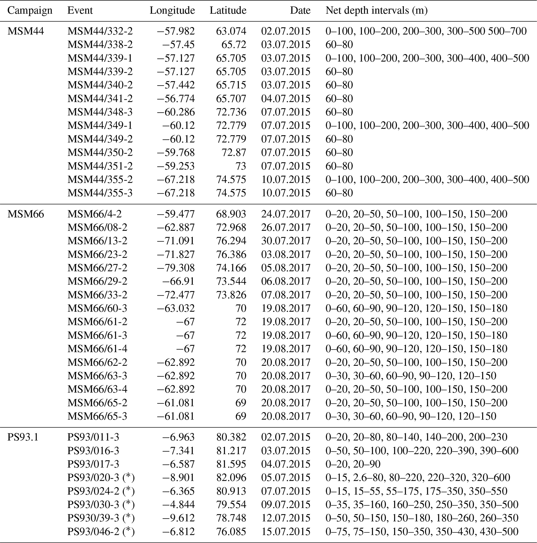
This study is based on a combination of existing and new data from vertically resolved profiles of plankton net samples from the Arctic Ocean and adjacent seas (Table 1; Fig. 1). We used all data from the studies by Kohfeld et al. (1996), Bauch et al. (1997), Kohfeld (1998), Volkmann (2000b), Stangeew (2001), Schiebel (2002), Simstich et al. (2003), Pados and Spielhagen (2014), and Greco et al. (2019), containing information on at least one of the three parameters, abundance, shell size or weight : size ratio of the planktonic foraminifera N. pachyderma, resulting in a dataset of 112 depth profiles. As data on shell size and weight, which are important for estimates of calcite mass flux, are scarce in existing publications, we have extended the dataset by 36 new vertical profiles taken during expeditions in Baffin Bay (MSM44, July 2015, and MSM66, July 2017) and in the Fram Strait (PS93.1, July 2015) (Table 2, Fig. 1). All of the new profiles consist of samples from five depth intervals (Table 3), sampled with a multiple closing plankton net (Hydro-Bios, Kiel) with an opening of 0.25 m2 and a mesh size of 100 µm during the MSM44 and MSM66 cruises and 55 µm during PS93.1. Shell number concentrations of various planktonic foraminifera species from five depth profiles from PS93.1 are published in Greco et al. (2021b). Here we recounted the number of shells of N. pachyderma in those profiles, generated new counts from three further profiles in the same expedition (PS93/011-3, PS93/016-3, PS93/017-3), and added measurements on shell size and weight on shells from all eight profiles.

Figure 1Overview of the research area with different regions (circled in red) sampled during different research cruises. Published data (orange) and new data (red) used in this study, as well as the sampling periods (symbols), are marked. Land and glacier polygons from Natural Earth Data (CC0) and bathymetry from Amante and Eakins (2009), using ggOceanMaps in R (Vihtakari, 2021).
Table 1Overview of the used samples of vertical plankton net data of N. pachyderma. At M21/4 and M21/5, the profile numbers in brackets indicate the number of individually labelled and taken profiles, which were combined into fewer profiles due to sampling at the same position at different depth intervals, as indicated by the number before the brackets. (Last access for all PANGAEA links is 30 May and 30 April 2022.)
Samples from Baffin Bay were either processed on board or stored at −80 ∘C until processed onshore. All foraminifera were manually removed from each sample and counted. The counts were made separately for cytoplasm-bearing shells and empty shells, differentiated during the processing of the wet samples. As recently deceased foraminifera can still contain cytoplasm, this leads to a bias in the numbers in favour of individuals interpreted as being alive upon sampling. Shell size (maximum diameter) was measured with the software ImageJ on pictures taken through a SteREO Discovery.V8 microscope.
Samples from the Fram Strait were stained using a Rose Bengal and ethanol (96 %) mixture to enable the differentiation of empty and cytoplasm-bearing shells. The samples were stored at 4 ∘C until processing. They were then washed over a 250 and 63 µm sieve. The residues were dried on filter paper, and the foraminifera were separated from the dried residues. In accordance with data from earlier studies, white or transparent shells were classified as empty (e.g. Fig. 2e) and all other (pink) shells as cytoplasm-bearing (e.g. Fig. 2f), assumed to represent specimens that were alive during retrieval. As rose Bengal might be staining recently dead specimens because of remaining cytoplasm in the shells (Schönfeld et al., 2013), there is a possible bias towards numbers of cytoplasm-bearing shells that are too high. Maximum shell diameter, perimeter and area of the two-dimensional cross-section of each individual in the umbilical view were measured with a KEYENCE VHX-6000 digital microscope. As heavily calcified shells of N. pachyderma tend to be less lobate than non-encrusted specimens, the ratio of perimeter and area can indicate the foraminifera shell shape (Fig. 2e–g): the more calcified the shell, the lower the ratio. The total weight of all shells was determined for each sample separately for shells that were considered empty and those that were considered cytoplasm-bearing, using a Sartorius SE2 ultra-micro balance (nominal resolution of 0.1 µg). The ratio between the total weight and the mean maximum diameter (size) is here used as an indicator of the mean calcification intensity. Upon sampling, no direct differentiation between shells with or without a crust was done. Encrusted shells are identified by their larger weight than non-encrusted shells, different shell texture and less lobate shape (Fig. 2g).
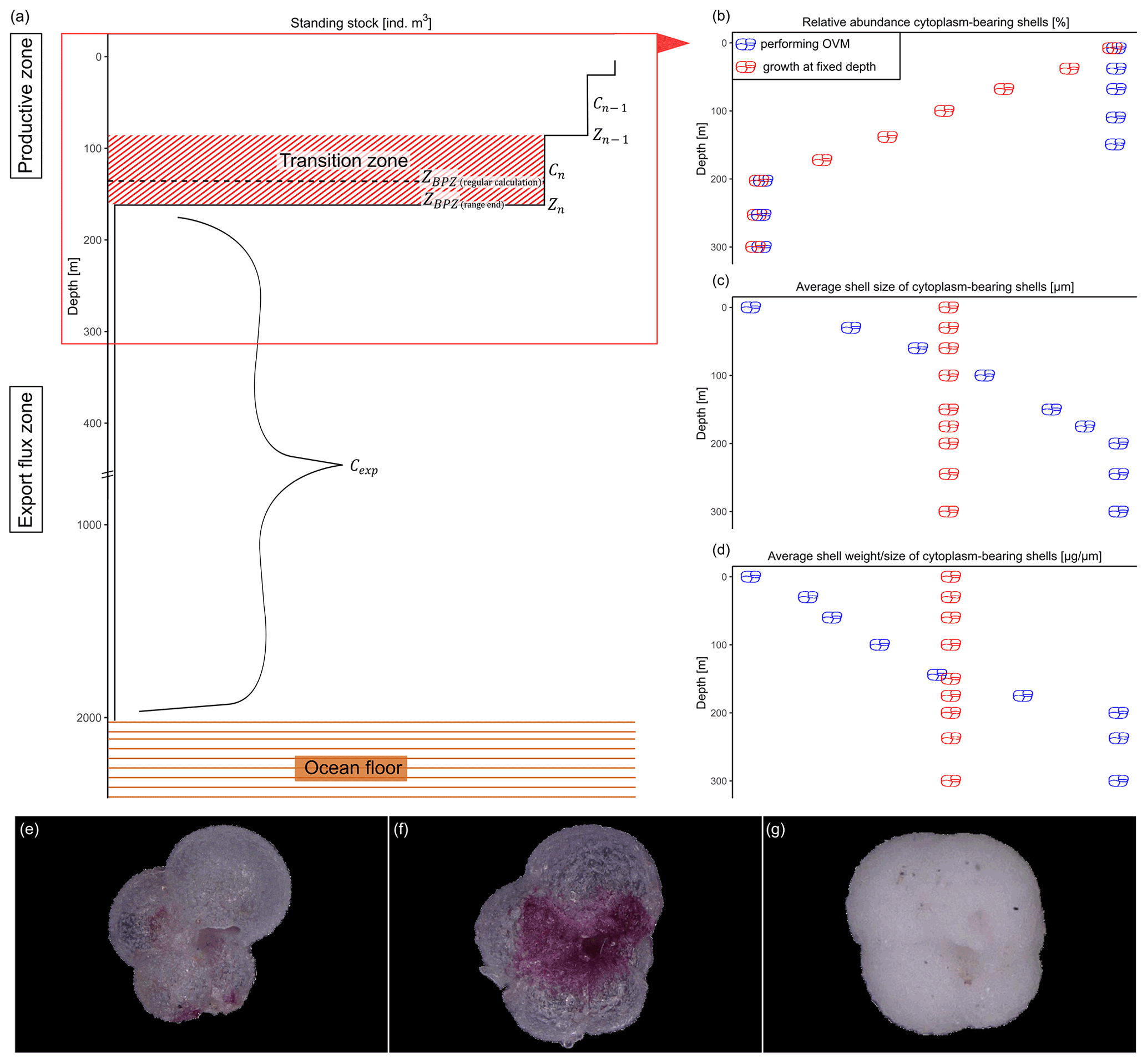
Figure 2Schematic overview of the studied shell parameter. Shown values are constructed numbers to represent the concept of the study and unmeasured values. (a) Change in standing stock of planktonic foraminifera with increasing depth. The parameters used to calculate the base of the export zone (ZBPZ) after Lončarić et al. (2006) are shown: the transition zone represents the area in which the foraminifera shell abundance (Cn) rapidly changes, with rather stable abundances in the area below (Cexp). Zn and Zn−1 represent the start and end depths of the transition zone, in which the calculated BPZ is located. For details on the calculation, see Sect. 2.2. Panels (b), (c) and (d) show the change in average (b) relative abundance of cytoplasm-bearing shells, (c) average shell size and (d) average calcification intensity (shell weight size) of cytoplasm-bearing shells with increasing water depth within the productive zone. Blue symbols represent the ideal situation if N. pachyderma performs ontogenetic vertical migration (OVM) throughout its life cycle, while red shell symbols indicate the expected trend when individual specimens grow their shell at a fixed depth. Panels (e), (f) and (g) show different types of encrustation of N. pachyderma, with (e) representing a non-encrusted shell, (f) the beginning of encrustation and (g) thick encrustation with a clearly different and more rounded shape.
2.2 Productive zone
To determine the depth range where shell calcification occurred and below which the export began, the base of the productive zone (BPZ) of N. pachyderma was defined for each profile by considering the changes in shell abundance with depth. Following the concept of Peeters and Brummer (2002), the BPZ is the depth where the shell abundance begins to substantially decline. It was calculated after Lončarić et al. (2006):
where Cn is the concentration of shell numbers within the transition zone (i.e. the last depth interval before the rapid decline in shell abundance), which was defined visually for every profile as exemplarily shown in Fig. 2a, Cexp is the average shell abundance, weighted by the thickness of the sampled depth interval at all depths below Cn, and Cn−1 is the foraminifera abundance in the depth interval above Cn. Zn represents the top of sampling depth of the transition zone and Zn−1 its bottom.
The equation applies to cases where the shell number concentration decreases with depth. Where this is not the case (such as where there is a distinct subsurface maximum), the equation cannot be used, as the estimated BPZ would appear to lie below the depth interval of the transition zone. This was the case in 37 out of 126 profiles. In addition, in three profiles, the transition zone corresponded to the uppermost sampling layer, and the equation could not be applied. For those 40 profiles, the BPZ was defined as the bottom depth of the transition zone (Fig. 2a, ZBPZ (range end)). This can result in a bias towards the estimated BPZ being located below the actual position. This bias is restricted by the overall sampling interval (median: 50 m) and has no effect on our flux estimates which are based on average shell abundances below the BPZ. In 10 profiles, calculation of the BPZ was not possible as no clear transition zone was present within the sample range, including two profiles in which the abundance was zero at the total station. The maximum sampling depth of those profiles was between 180 and 300 m, implying that the transition zone either occurred in the bottom interval or was not yet reached. Because of this ambiguity, these profiles were not used for the BPZ analysis. For profiles where abundance data were available for only one or two depth intervals at the surface (nine profiles), estimation of the BPZ was not possible either. In total, the BPZ was determined in 126 profiles, and the different methods to define BPZ were separated in the interpretation. For an overview of the number of profiles that were available for the different calculations, see Table 2.
Table 2Overview of the numbers of depth profiles used in the study, with varying numbers depending on the studied parameter.

The above definition of the BPZ does not rely on the separation of living (cytoplasm-bearing) and dead (empty) shells during sampling, a parameter that was not systematically recorded. The separation is ambiguous, as cytoplasm decomposition takes time after death, and individuals already dead could still be considered as living due to the presence of residual cytoplasm (Schiebel et al., 1995). This ambiguity is larger at greater depth, where the probability of finding living specimens becomes smaller. Nevertheless, where available, we used the proportion of cytoplasm-bearing and empty shells as another indicator of the maximum extent of the productive zone.
To investigate at which depth of the productive zone the calcification of N. pachyderma occurred and if the species performed OVM, we considered the vertical profiles of the following parameters: (i) relative abundance of empty shells, (ii) shell size and (iii) mean calcification intensity expressed as the shell weight : size ratio. The reason for using those parameters is that if N. pachyderma performed OVM and premature mortality were zero, empty shells would only be present at the bottom of the productive zone, where the specimens would reach their maturity, while the abundance of cytoplasm-bearing shells would be 100 % at all depths above (Fig. 2b). At the same time, shell size and calcification intensity would increase constantly with increasing depth, reaching maximum values only at the base of the productive zone. In contrast, if individual specimens did not migrate during their life cycle, the fraction of the population dying would be equal across the productive zone. Assuming that empty shells only sink, this would lead to a linear decrease in relative abundance of cytoplasm-bearing shells. Because foraminifera of any life stage would be present in equal proportions at all depths, the average shell size and weight of cytoplasm-bearing specimens should stay constant with increasing depth (Fig. 2b–d).
Table 3Overview of the sampled depth intervals from the stations of MSM44, MSM66 and PS93.1. Abundances of N. pachyderma of profiles marked with (*) are also published in Greco et al. (2021b), but counts presented in the studies were done independently from that publication.
2.3 Export flux zone
When the bottom of the productive zone is known (or estimated), the abundance of shells below that depth can be used to estimate the export flux by taking the sinking velocity into account (Schiebel and Hemleben, 2000). Assuming that the organic matter content of foraminifera is negligible, the calcite flux can subsequently be calculated using (average) shell weight:
where shell weight is the measured average weight of shells below the productive zone, as these are representative of the export flux. Whenever possible, the measured average shell weight was used, but for samples where no weight data are available, we used regional mean values. In regions where some weight data were available (Fram Strait, Labrador Sea, Greenland Sea, Norwegian Sea), average weights were calculated from samples of those regions alone. In all other regions, the overall mean weights from our data were used. This method is likely to underestimate present variability. To evaluate possible effects on mass flux from distinct shell types, fluxes based on average weights of either only encrusted and empty or non-encrusted and cytoplasm-bearing shells from below the productive zone were calculated as well. Shell abundance was calculated as the number of shells, divided by the sampled depth range and multiplied by the area of the net opening (as an estimate for the volume of sampled water). Sinking velocity was calculated after Takahashi and Bé (1984):
using the same (average) weights as described above.
The residence time of N. pachyderma in the productive zone was then estimated based on the standing stock within the productive zone (individuals per square metre: ind. m−2) divided by the shell flux (ind. m−2 d−1).
2.4 Statistical analysis
Statistical analyses were performed using R v. 3.6.1 (R Core Team, 2018). To compare measured parameters between cytoplasm-bearing and empty shells, Welch's t test was performed. The analysis of trends within the productive zone was done within the range calculated individually beforehand of the productive zone of the stations. Linear regression models were used to detect the effects of depth and sampling location on the different parameters. As the data of shell size and calcification intensity are not normally distributed, they were log-transformed before these analyses. Since the depth of the BPZ varies among the profiles, analyses were performed using tow intervals standardized to the depth of the productive zone. Some intervals extend to below the BPZ. In these cases, the tow interval represents > 100 % of the depth of the productive zone.
3.1 Shell abundances and the productive zone
The average shell abundance of N. pachyderma in our dataset is 25 ind. m−3 (Table 4). Shell abundances show a maximum either within the upper 50 m or in the depth zone below, reaching down to 150 m (example shown in Fig. A1). Those distinct patterns are distributed rather equally among all profiles and regions. Below the depth of maximum shell abundance, there is a rapid decrease in all profiles until the abundances stabilize above 300 m water depth.
Empty shells of N. pachyderma are present across the entire sampled depth range (Fig. 3a). In the majority of the profiles, the BPZ is located between 100 and 150 m (Fig. 3b). Based on the calculation after Lončarić et al. (2006), the median BPZ is situated at 124 m water depth. At stations where the BPZ could only be defined as the end of the depth range of the transition zone, its median depth is 136 m. Irrespective of how calculated, the BPZ varies among different stations and regions, with the lowest median water depth of 100 m in Baffin Bay and the highest median value of 160 m in the Barents Sea (Table 4), with variability within the regions being as large as among the regions. The minimum calculated BPZ is 15 m in a profile from the Fram Strait (PS93/020-3), and the minimum BPZ determined by the end of the net range is 20 m in a profile from Baffin Bay (MSM09/2 466-2). The deepest BPZs reach 300 m and correspond to the pattern visible in the relative abundance of empty shells (Fig. 3a). Within the productive zone, the average shell number concentration of N. pachyderma is 42.27 ind. m−3; below the productive zone, it is 6.52 ind. m−3 (Table 4).
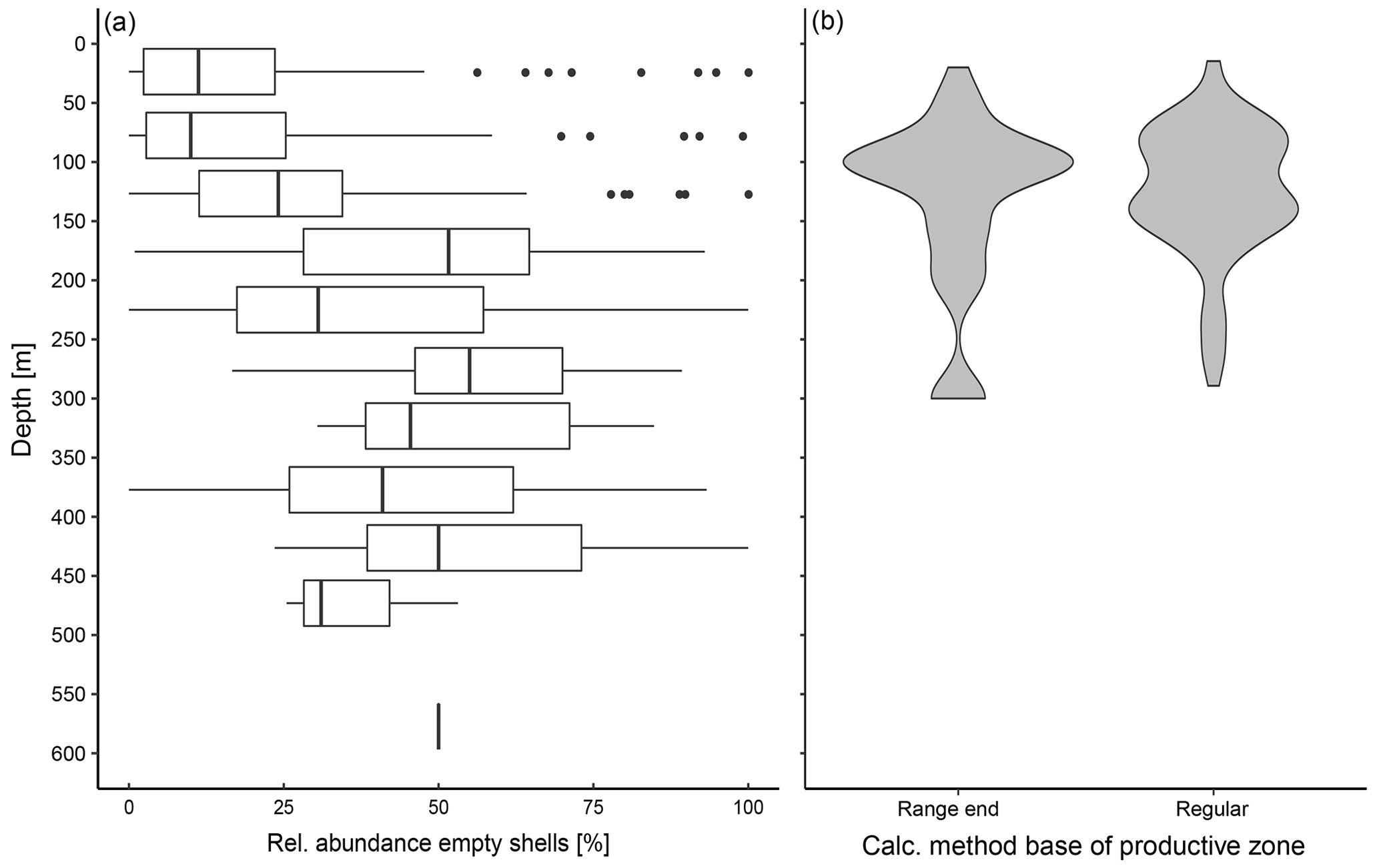
Figure 3(a) Vertical profile of relative abundance of empty shells at all stations of the study in which empty and filled shells were distinguished. The boxes represent the interquartile range (IQR) of the relative abundance at the given depth, and the vertical bar represents the median. Outliers, shown as points, are values beyond 1.5 × IQR of each site of the box, and lines represent the range within 1.5 × IQR. The line at 600 m depth represents the abundance of empty shells in one single sample, as sampling in all other stations did not reach to that depth. (b) Range of the base of the productive zone (BPZ), divided by the way they were determined: “range end” shows all samples in which the maximum depth of the net of the transition zone was defined as the BPZ, while “regular” shows all samples in which the equation from Lončarić et al. (2006) to estimate BPZ could be applied, as described in Sect. 2.2.
Table 4Overview of measurements on different shell parameters from the different sampling areas of the study. Next to each indicated value, the 95 % confidence interval (CI) is given in italics. It is calculated assuming normal distribution, and the number of samples (n) used to calculate each parameter is given in brackets.
3.2 Shell sizes
The average maximum diameter of N. pachyderma in our samples is 150 µm (Table 4). Shells from Baffin Bay with a mean size of 146.5 µm (sampling mesh size: 100 µm) are smaller than shells from the Fram Strait (only data from PS93.1) that have a mean size of 180 µm (sieving size: 63 µm; Table 4, Fig. 4). Welch's t test shows that this difference is significant (p < 0.001). Cytoplasm-bearing shells within the estimated productive zone of each station in samples from PS93.1 are on average bigger than empty ones (mean sizes of 188.2 and 166.2 µm, respectively; Fig. 4a). Welch's t test shows that this difference is significant in 8 of 14 individual samples (p ≤ 0.006). At station PS93/024-2 in the topmost net (0–15 m), empty shells were significantly bigger (p = 0.035) than cytoplasm-bearing ones. Below the productive zone, 2 of 16 individual sampling positions contain empty shells that are on average significantly bigger than those filled with cytoplasm (p < 0.01). In all other samples, the differences were not statistically significant. In both regions, shells below the productive zone are significantly, if only slightly, bigger than within the productive zone (Welch's t test: p < 0.001), with averages of 150 and 153 µm, respectively (Fig. 4b). Statistical analysis indicates that there is no significant linear increase in average size within the productive zone (Fig. 5; Baffin Bay: p = 0.399; Fram Strait empty: p = 0.199; Fram Strait cytoplasm-bearing: p = 0.627). We find no evidence for lunar periodicity in the shell size of N. pachyderma in our samples.
Figure 4Overview of shell sizes of N. pachyderma from the Fram Strait (blue) and Baffin Bay (orange), contrasting empty, cytoplasm-bearing and non-determined shells (a) within the productive zone and (b) in the export flux zone. Shell types are also not distinguished in (b) in samples from the Fram Strait, as we assume all shells collected below the productive zone to represent specimens that were dead during retrieval. The boxes and bars represent the interquartile range as explained in the caption of Fig. 3.
3.3 Shell calcification intensity
Across both new data and literature data, the mean shell weight of N. pachyderma per sample ranges from 0.1 µg (potentially referring to fragments of shells from the Fram Strait, data from Kohfeld, 1998) to 20.8 µg (shells from the Labrador Sea, data from Stangeew, 2001). The overall average weight is 3.4 µg (median: 2.3 µg; Table 4) and the average calcification intensity (weight size) 0.013 µg µm−1 (median: 0.010 µg µm−1). Shell weight and calcification intensity of non-encrusted shells are lower than of (heavily) encrusted shells. Similarly, cytoplasm-bearing shells are lighter and have a lower calcification intensity than empty shells (Fig. 6). The differences become smaller below the productive zone. Welch's t test shows that the difference between the calcification intensity of cytoplasm-bearing and empty shells from PS93.1 is significant, both within (p < 0.001) and below (p = 0.004) the productive zone, with empty shells being always stronger calcified.
Figure 5Mean of difference in mean shell size at the individual station and depth and the overall mean of the station, plotted against the percentage of the depth interval on the overall depth of the productive zone. 100 % equals the total depth of the productive zone and 50 % half of the depth of the productive zone. More than 100 % is reached where the sampling interval ends below the BPZ. The plot is divided into different types of shells (undetermined, empty, cytoplasm-bearing) and the two regions from which size measurements are present (Baffin Bay, Fram Strait). Consider that the samples do not represent all samples from the region shown in Fig. 1 but only those from (a) MSM44 and MSM66 and (b, c) PS93.1. The red line indicates the position at which no difference between the mean of the depth and the overall station exists. Only the depth interval within the estimated productive zone of each station is shown. The p values show the effect of the increasing proportion of the productive zone on shell size.
Figure 6Overview of (a) average shell weight and (b) calcification intensity (weight size) from shells with a different status. In this study (1), differentiation was made between cytoplasm-bearing and empty shells on shells ≥ 63 µm, while Kohfeld (1998; shells ≥ 150 µm; (2)) and Stangeew (2001; shells ≥ 63 µm; (3)) distinguished between (heavily) encrusted and non-encrusted shells. Besides, different sampling regions are distinguished. Blue boxes show the parameter within the productive zone of each station and orange boxes the values from samples taken below the estimated productive zone of each station. The boxes and bars represent the interquartile range as explained in the caption of Fig. 3.
Shell size parameters can be used to infer the presence of crust by a less lobate periphery (Fig. 2e–g) in samples where it has not been checked visually: lower perimeter : area ratios indicate rounder, likely more encrusted shells. Indeed, both within and below the productive zone, empty shells from PS93.1 are significantly rounder than cytoplasm-bearing shells (Welch t test, p < 0.001), suggesting that empty shells are more encrusted than cytoplasm-bearing shells (Fig. A2). We observe no statistically significant difference in the roundness of shells between cytoplasm-bearing shells within and below the productive zone (p = 0.9), but empty shells from below the productive zone are significantly rounder than those within the productive zone (p < 0.001; Fig. A2). While differences within samples from the Fram Strait could be partly due to differences in sampling methods among the different studies and authors, large regional differences between the Fram Strait, the Greenland Sea and the Labrador Sea (Fig. 6) are likely reflecting real variability because many of the involved studies used the same methodology.
A total of 10 out of 18 profiles show a clear tendency towards higher calcification intensity with depth (Fig. 7). In seven profiles, no clear trend with depth can be detected in calcification intensity. Those profiles are all from the samples of PS93.1: four of them of empty and three of cytoplasm-bearing shells. One profile of non-encrusted shells from the Fram Strait shows lower calcification intensity at deeper depth. The involved sample size is too small to allow statistical analysis.
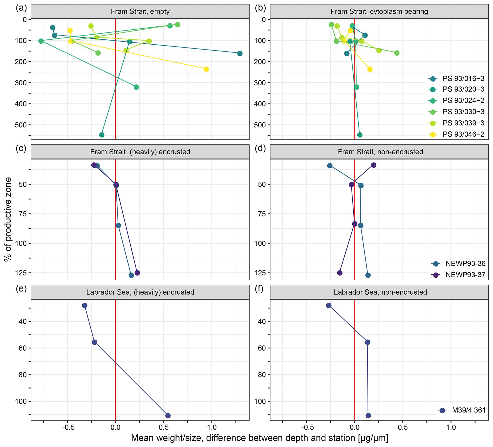
Figure 7Mean of the difference in average calcification intensity (weight size) at individual stations and depths and the overall weighted mean of each station within the productive zone, plotted against the percentage of the depth interval on the overall depth of the productive zone. 100 % equals the total depth of the productive zone and 50 % half of the depth of the productive zone. More than 100 % is reached where the sampling interval ends below the BPZ. Differentiation of shell types is done between cytoplasm-bearing and empty shells from Fram Strait samples of this study (a, b), while Kohfeld et al. (1998) (c, d) and Stangeew (2001) (e, f) distinguished between (heavily) encrusted and non-encrusted shells in samples from the Fram Strait and the Labrador Sea. The red line indicates the position at which no difference between the mean of the depth and the overall station exists, and different colours are used to make the shape of change in individual profiles visible.
3.4 Shell mass flux
The overall mean calcite mass flux of shells of N. pachyderma below the BPZ in each profile based on actual weights or, where not measured, average weight of shells from below the productive zone is 8.0 mg CaCO3 m−2 d−1 (20.1 mg CaCO3 m−2 d−1 based on weights of encrusted and empty shells only; 4.5 mg CaCO3 m−2 d−1 based on weights of non-encrusted and filled shells only; in the following, those two values will always be given in brackets without further stating this specification). Although in some profiles, the flux seems to increase further below the BPZ, the majority of the profiles shows almost no change or a decrease in mass flux (Fig. 8). When calculated for shell number concentrations at the deepest net of each profile, the average calcite mass flux is further reduced by a half to 4.4 mg CaCO3 m−2 d−1 (10.7; 2.4 mg CaCO3 m−2 d−1). The average loss rate in fluxes of CaCO3 from the net below the base of the productive zone and the deepest sampling position of each profile is 6.6 % per 100 m (8.9 % per 100 m; 9.5 % per 100 m), the median loss is 9.1 % per 100 m (19.4 % per 100 m; 19.4 % per 100 m). The highest variations and most extreme values of changes with depth are present in Baffin Bay, the Fram Strait and the Labrador Sea (Fig. A3). Scaling the calcite mass loss for every pair of depth intervals below the BPZ (Fig. 9b) reveals that high values (and high variability of values) are limited to the 300 m depth interval below the BPZ, with both mean values and variability decreasing with depth. Weight measurements from the profiles of PS93.1 indicate that this loss is both driven by a decrease in shell mass and shell number concentration (Fig. 9a).
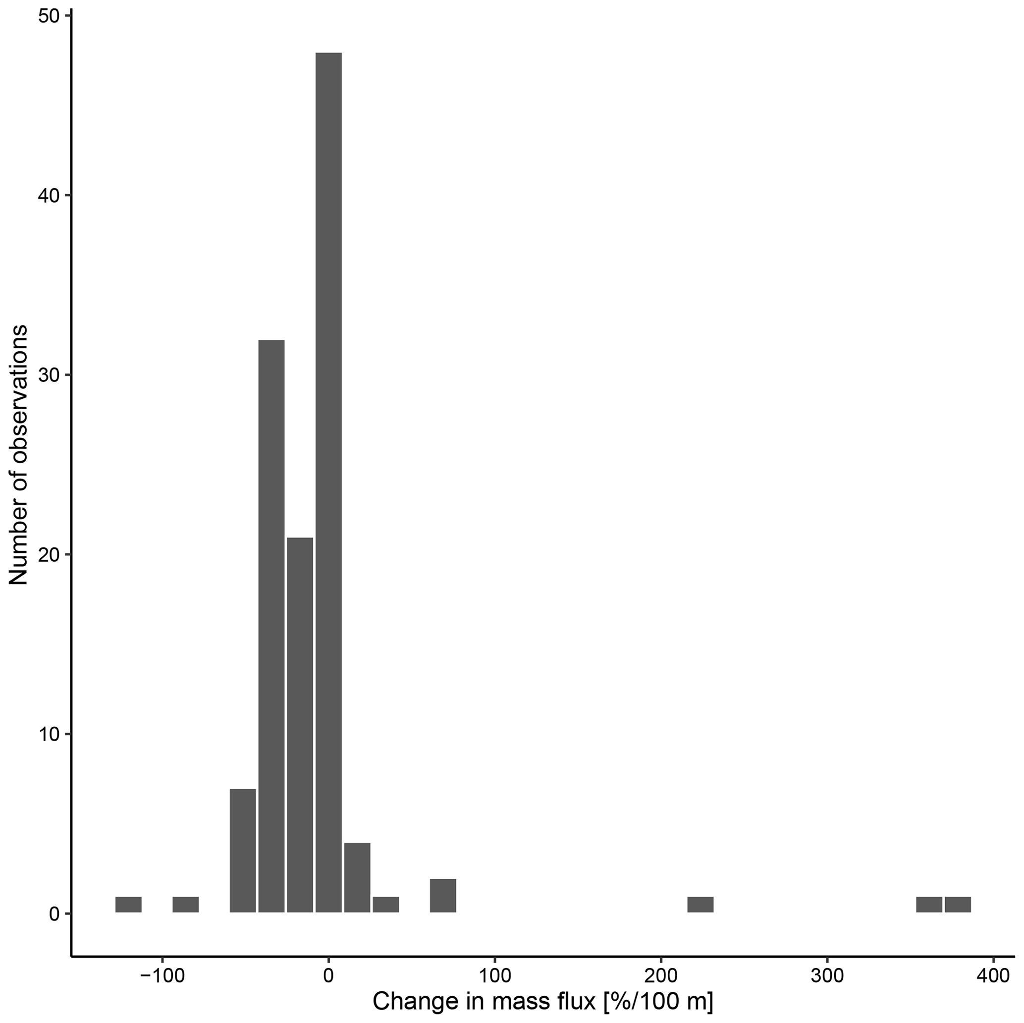
Figure 8Change in mass flux between the net directly below the calculated base of the productive zone and the deepest net of sampling of each station.
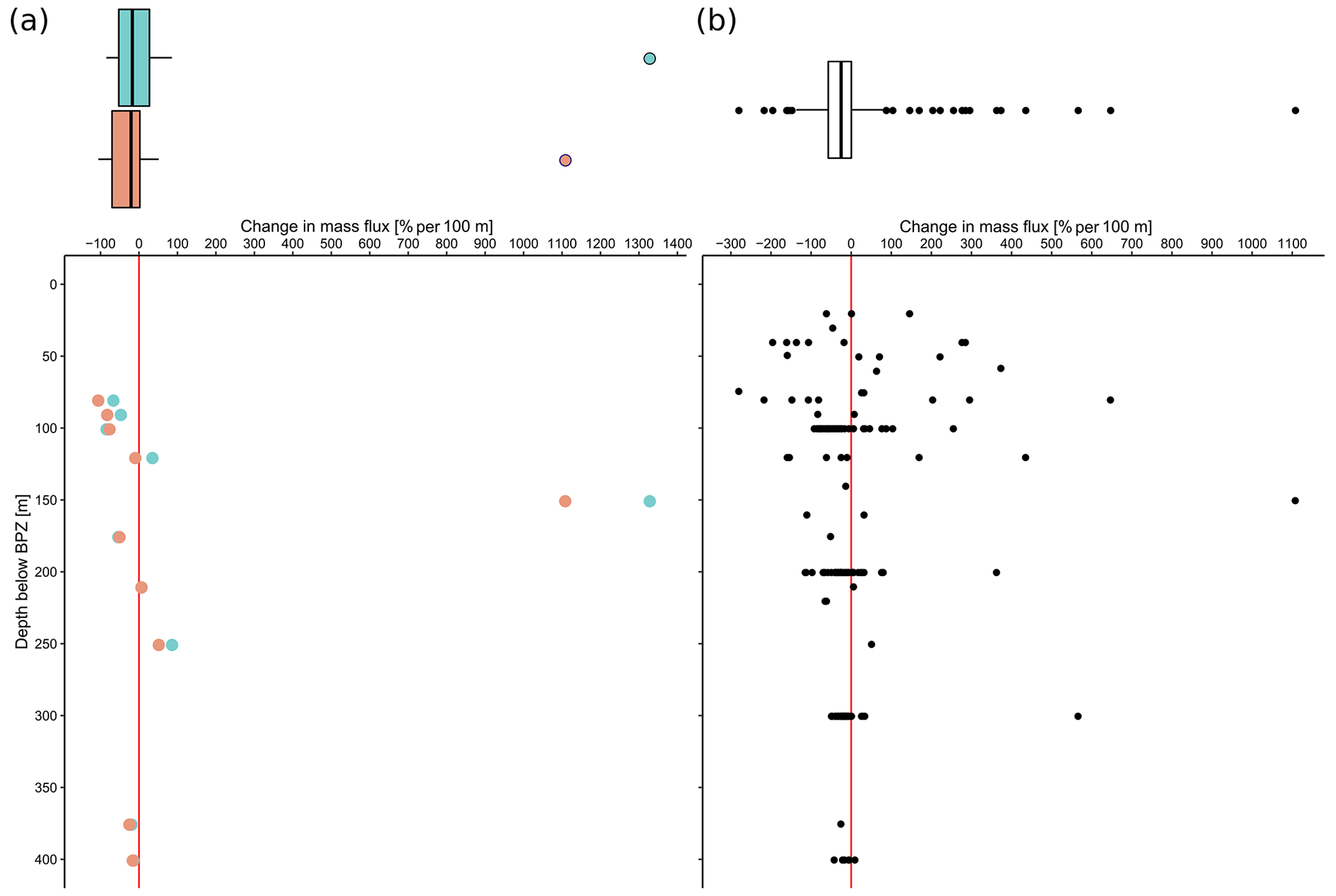
Figure 9Flux loss with depth per 100 m (in %), calculated between different sampling intervals located below the interval including the base of productive zone, plotted against the distance between the maximum sampling depth of the individual interval and the end of the net including the base of the productive zone. Panel (a) is a comparison of loss in shell number concentration (blue) and shell mass (orange) in PS93.1 samples from the Fram Strait, and (b) shows the loss in mass flux of all samples, estimated based on average shell weight and shell number concentration. The boxes and bars on top of the plots represent the interquartile range as explained in the caption of Fig. 3 and are plotted against the same x axis as the plot below.
Irrespective of how (at which depth) the flux was calculated, the estimated mass fluxes varied among the 147 profiles by more than 3 orders of magnitude (Fig. 10). This variability has some regional components: the highest flux below the productive zone (156.9, 398.6, 83.4 mg CaCO3 m−2 d−1) was determined for a station in the central Baffin Bay (Fig. 11a). In the Greenland Sea, some stations also show high values (fluxes with a maximum of 66.64 mg CaCO3 m−2 d−1 based on individual measurements). Those two regions have the highest average fluxes (both about 20 mg CaCO3 m−2 d−1 at the base of the productive zone based on individual measurements). In comparison, average fluxes are low in the Barents Sea, Fram Strait, Labrador Sea, Laptev Sea and Norwegian Sea (< 5 mg CaCO3 m−2 d−1; Table 4).
3.5 Residence time
The calculated residence time of N. pachyderma based on standing stock within and shell fluxes below the productive zone ranges from < 1 to 79 d, excluding three extreme values of 182 (MSM09/2 455-7, Baffin Bay), 373 (M21/4 MSN697 and MSN698, Norwegian Sea) and 655 d (M39/4 366, Labrador Sea) (Fig. 12). The median residence time is 4 d (1.8 d using average weights of encrusted and empty shells; 3.1 d using average weights of non-encrusted and cytoplasm-bearing average weights for the calculation of shell flux, in which sinking velocity based on shell mass is incorporated). The 95 % confidence interval ranges from 3 to 5.1 d (1.2 to 2 d (encrusted and empty); 2.2 to 3.5 d (non-encrusted and cytoplasm-bearing)), with a geometric mean of 3.9 d (1.5 d (encrusted and empty) 2.8 d (non-encrusted and cytoplasm-bearing)).
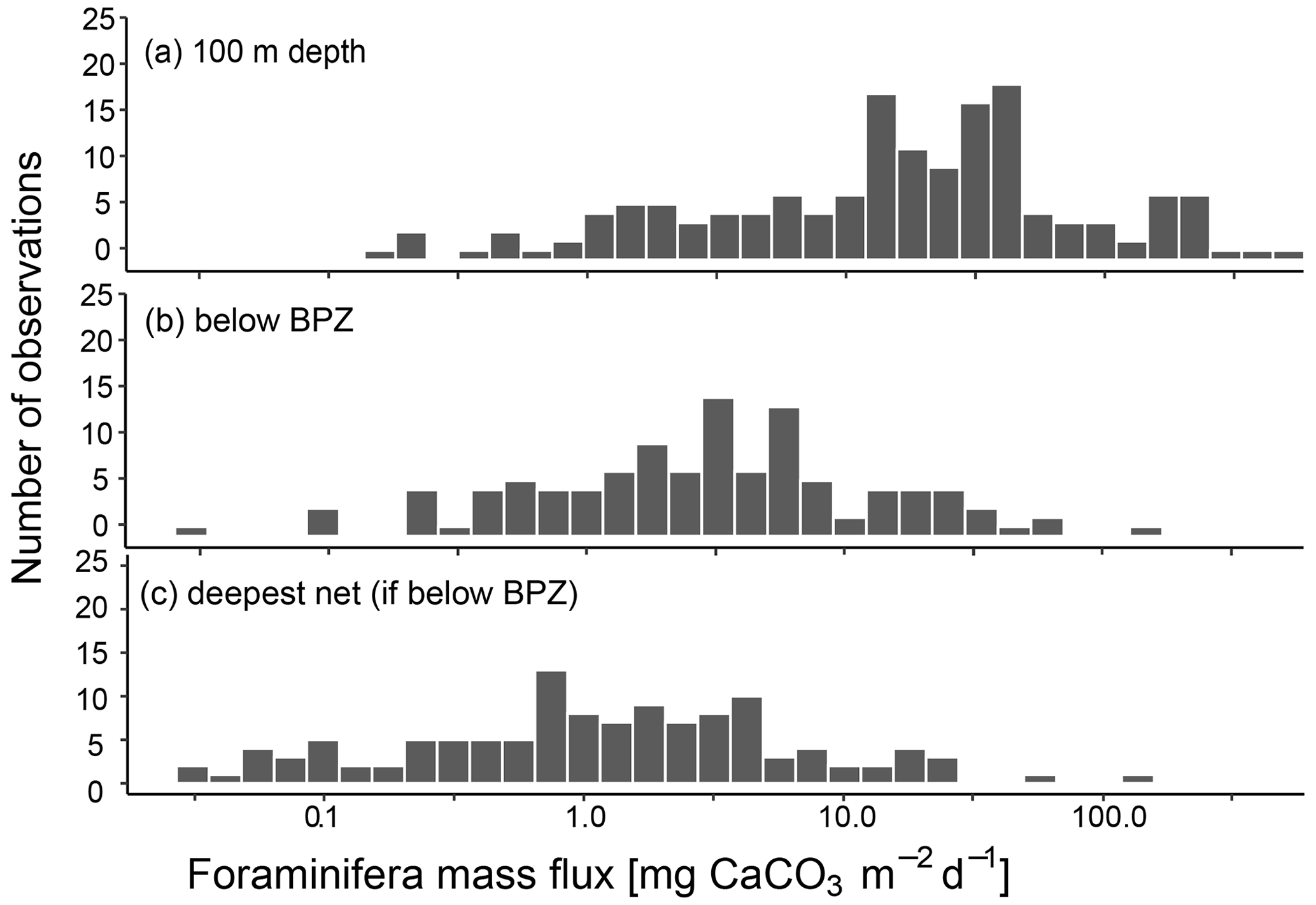
Figure 10CaCO3 mass flux of planktonic foraminifera N. pachyderma, calculated based on shell weights of individual samples and, where no weight measurements are present, based on average weights from the region or all samples included in this study. Consider the logarithmic scale of the x axis. Panel (a) shows the fluxes at around 100 m depth (maximum sampling depths of nets: 75–100 m), (b) the flux in the net below the calculated base of productive zone (BPZ) of the individual stations and (c) at the deepest net of each station including all stations where that is located below the BPZ. The exact width of sampling intervals differs between individual sampling locations. Details on this are shown in Table 3 for profiles added in the study and in the references listed in Table 1.
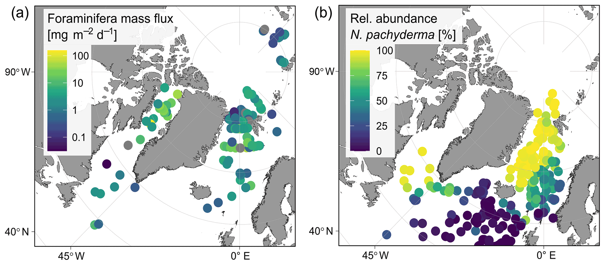
Figure 11Regional overview of (a) foraminifera CaCO3 mass flux of planktonic foraminifera N. pachyderma during summer (sampling period from June to September, varies among stations as shown in Fig. 1) below the estimated productive zone. Fluxes were calculated based on shell abundances determined in plankton net samples. Shell weights are either from direct measurements or based on average weights from the region of sampling. Consider that values are plotted on a logarithmic scale to visualize the huge regional variability. Panel (b) shows the relative abundance of the species N. pachyderma found in sediment cores (data from ForCenS dataset, Siccha and Kucera, 2017).
4.1 Productive zone and export flux zone
Our analysis of observations from plankton net samples indicates that the productive zone of N. pachyderma in the Arctic and Subarctic realm reaches down to about 113 m water depth (median of all samples: 125 m for where the calculation after Lončarić et al. (2006) was possible and 136 m where it was defined as the range end). Greco et al. (2019) have shown that the habitat depth of N. pachyderma varies substantially. A variation in the depth interval of maximum abundances of N. pachyderma is also presented by Carstens and Wefer (1992) and Carstens et al. (1997), where a connection between distinct water masses and temperature regimes is drawn. Our dataset corroborates these observations and indicates that the base of the productive zone of N. pachyderma is also highly variable and reflects the habitat depth (vertical distribution of living specimens). Like Greco et al. (2019), we observe that even if there would be a general pattern of habitat depth and BPZ position being driven by environmental factors, as also proposed by Carstens et al. (1997), it is overlain by considerable variability, even among profiles collected in the same region and around the same time. This means that the observed BPZ variability cannot be driven by the water-column structure alone.
Some of the variability in the BPZ estimates may reflect patchiness in the distribution of planktonic foraminifera populations (Siccha et al., 2012). Meilland et al. (2019) observed that a patchy distribution is mainly present on a horizontal scale, with vertical distribution remaining rather stable. Nonetheless, a horizontally patchy distribution could affect the calculated BPZ in samples from the same region: in profiles with very low shell abundances (< 10 ind. m−3, sometimes even < 1 ind. m−3), the estimate of the BPZ position may be affected by non-representative estimates of population density. Thus, large abundance differences, caused by a patchy distribution, which has been reported to be best developed for species occurring with high abundances in the Arctic (Meilland et al., 2020), could cause large differences in estimated BPZ and display a variability in the results which may not be representative of the actual situation.
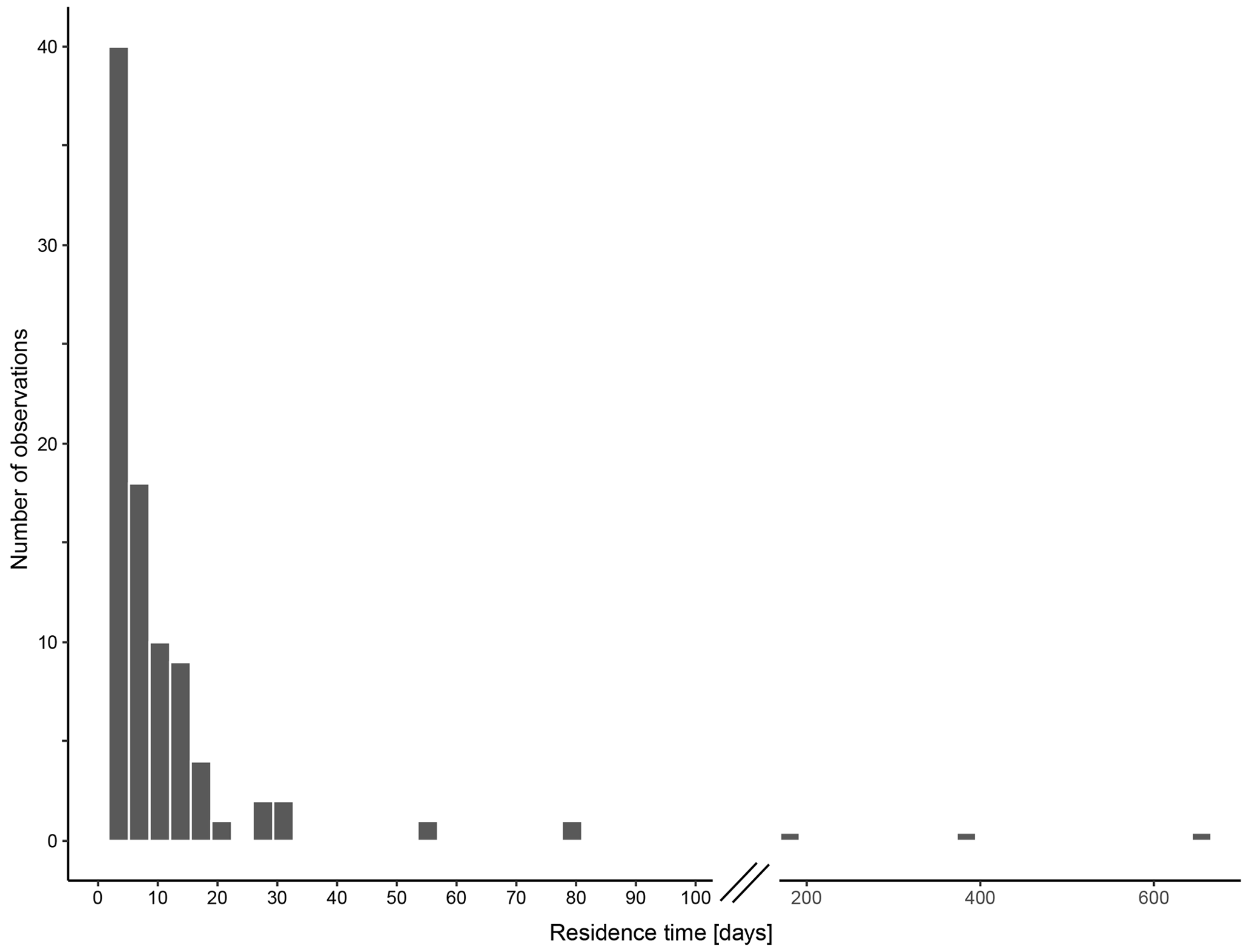
Figure 12Residence time of empty shells of N. pachyderma within the productive zone in days, calculated based on the standing stock within the productive zone and the shell flux below the base of the productive zone, calculated with average shall masses below the productive zone. Consider the break in the x axis between 100 and 200 d.
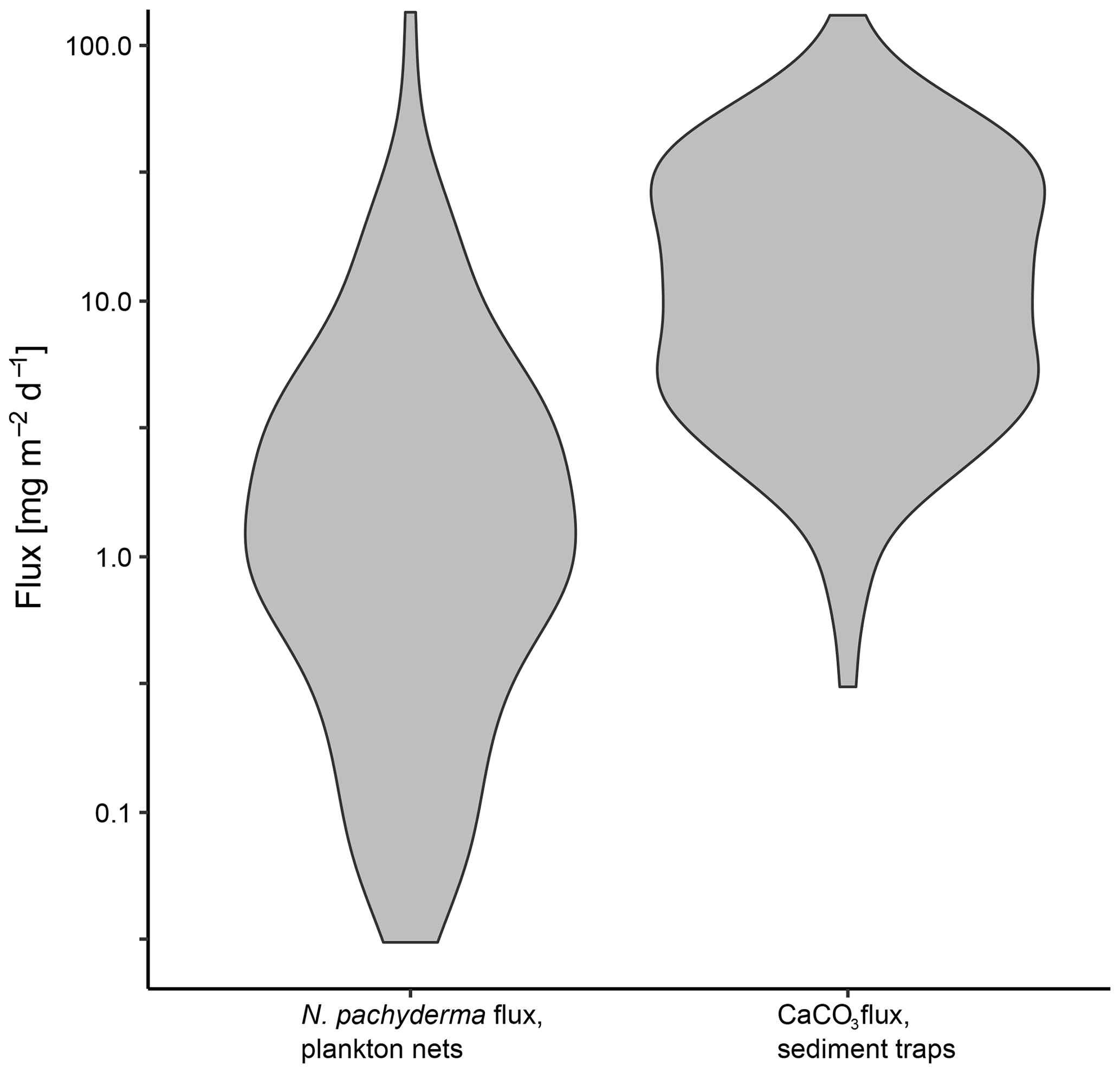
Figure 13Comparison of daily mass flux of N. pachyderma in plankton nets and CaCO3 in sediment traps plotted on a logarithmic scale. Sediment trap data are from sediment traps in the Fram Strait (Hebbeln, 2000; Bauerfeind et al., 2009), the Greenland Basin (von Bodungen et al., 1995) and the Lomonosov Ridge (Fahl and Nöthig, 2007).
In addition, the vertical resolution of the compiled plankton net profiles (15 to 175 m within the upper 300 m depth; Table 3) has a marked impact on the precision of the estimated position of the BPZ. Thus, some of the variability in the BPZ position could arise from differences in sampling methods. The BPZ estimate is also affected by the shape of the pattern of change in shell abundance with depth. Where the transition between the productive and the export zone is too gradual, the estimated depth of the BPZ is associated with larger uncertainty.
Some profiles show a pattern of an apparent gain in foraminifera mass flux below the inferred BPZ (Fig. 9). Our analysis of PS93.1 samples indicates that both higher shell abundances and shell weight below the productive zone are present at some of the stations. Higher shell weight could be explained by the loss of lighter, thinner shells due to dissolution, leading to a higher bulk weight at deeper depth. Gains in fluxes due to higher shell number concentrations are poorly constrained at depths below the BPZ, as the number of shells present in deeper nets is very low (Fig. A1a–e). A high percentage gain in flux might in some cases only represent a difference of a few shells, which is not related to an actual higher flux but to methodological uncertainties of sampling, and hence is not significant.
In summary, the calculated BPZ in each profile is associated with some uncertainty. However, the spatial variability in the position of the BPZ is larger than the uncertainty and hence a real characteristic of the ecology of N. pachyderma. The location of the BPZ below 100 m in many profiles and never below 300 m is robust considering the range in vertical sampling resolution (Fig. A1). Explicitly considering the variability in the depth of the BPZ increases the leads to improved estimates of the shell flux of N. pachyderma from plankton net samples.
4.2 Calcification depth
While empty shells are already present in the sampling intervals close to the surface and the relative abundance of empty shells tends to increase with increasing depth in the productive zone (Fig. 3), shell size does not systematically change with depth (Fig. 5). These observations speak against the presence of extensive OVM by N. pachyderma in the studied area (Fig. 2). This is consistent with observations of no clear change in shell sizes of the species with increasing depth in the Barents Sea presented by Ofstad et al. (2020). In contrast, Stangeew (2001) and Manno and Pavlov (2014) described higher abundances of small-sized shells in the upper water column close to the surface in N. pachyderma from the Fram Strait. However, even in those two studies, some large shells were present in surface samples. Plankton net data from the Nansen Basin from Carstens and Wefer (1992) show higher abundances of small-sized shells below 100 m depth, which the authors linked to the impact of different water masses in the area. Thus, different conditions at different water depths and/or within different water masses can influence both the abundances of planktonic foraminifera (Carstens et al., 1997) and their assemblage size distribution, which could lead to size differences at different depths. The lack of any pattern in shell size in our data does not provide an indication of OVM, and trends in size visible in other studies could in fact be driven by distinct water conditions and not or not alone by the performance of OVM. Our data also do not present a strong systematic change in size with lunar day, as was detected in previous studies (Schiebel et al., 2017). However, our shell size data do not cover the entire lunar cycle, preventing drawing firm conclusions on the influence of the lunar cycle on the shell size of N. pachyderma.
The likely important role of local environmental parameters on the terminal shell size is also reflected in the differences in shell size between empty and cytoplasm-bearing shells. Empty shells should be representative of specimens that have completed their life cycle. Therefore, shell growth at a constant depth throughout the life cycle of an individual should result in on average larger empty than cytoplasm-bearing shells at all depths. However, we only find such a difference in 1 of 14 samples, and on the contrary, significantly bigger cytoplasm-bearing shells occurred in 8 of 14 samples. On the other hand, the calcification intensity of empty shells is significantly higher than for shells bearing cytoplasm in all but one sample, and their shape is significantly more rounded, further indicating strong calcification. This shows that at least in the case of the studied N. pachyderma, shell size measured as the maximum diameter of the shell is not an ideal indicator for maturity but a highly variable parameter among individual specimens that might reflect variation in environmental conditions during the life cycle of the individual foraminifera. In contrast, the consistently observed stronger calcification intensity of empty shells at all depths and their distinct shape rule out that empty shells in the upper water column only represent specimens affected by premature death, i.e. before reproduction. The stronger calcification compared to cytoplasm-bearing shells is a clear indicator for a completed life cycle, as this species is known to often be associated with the development of a thick terminal calcite layer or crust (Bé, 1960; Kohfeld et al., 1996). In Stangeew (2001), where the presence of OVM is concluded based on shell sizes, the area of occurrence of strongly encrusted shells was observed to range from surface to 300 m depth, suggesting reproduction occurred across this whole depth range and not only at its base.
A total of 10 out of 18 of the profiles studied here indicate an increase in calcification intensity with increasing depth within the productive zone (Fig. 7), which would speak in favour of OVM. However, with the other half of the profiles not displaying any trend with depth, we must conclude that there is no clear signal for OVM being present or absent. If OVM would be present across all specimens of N. pachyderma in the Arctic and Subarctic realm, it would need to be very limited in the depth range to not be clearly visible in our data. In regions where the productive zone ranges from about 50 to 120 m water depth, the resolution of the studied vertical profiles might be not sufficient to detect it.
The occurrence of heavily calcified empty shells at all depths indicates that many specimens of N. pachyderma reach the final stage in their life cycle, building their final thicker crust, at all depths within their depth habitat. The same conclusion was also favoured by Kohfeld et al. (1996). These authors in addition hypothesized that the local conditions at a given depth not only affect the final size but also calcification intensity. Indeed, like size, calcification intensity in planktonic foraminifera has been shown to reflect parameters like temperature, productivity and optimum growth conditions (e.g. Weinkauf et al., 2016). Those parameters could also cause trends in the calcification intensity with depth, without necessarily being driven by strict OVM.
The sampling period of our data has to be considered when evaluating changes in size and calcification intensity with depth: depending on the life span of N. pachyderma, which could be longer than 1 or 2 months (Carstens and Wefer, 1992; Kohfeld et al., 1996), it is possible that the samples contain individuals from multiple generations that were produced during different environmental conditions. Furthermore, sinking shells of N. pachyderma can be transported over considerable distances, as, for example, shown by von Gyldenfeldt et al. (2000), whose results would indicate a transport of 25–50 km in the upper 1000 m, resulting in the possibility of some of the encountered specimens being advected from areas with a different hydrography. Because environmental conditions can have an impact on shell size and calcification intensity (e.g. Weinkauf et al., 2016), advection could blur signs of OVM if the life span of N. pachyderma is long relative to the speed of advection. Even though the residence time is not a direct measure of life span, since it only reflects the average time that foraminifera > 90 µm spent alive in the productive zone and hence excludes the time it takes to reach maturity, it can provide a first-order approximation. The majority of the estimated residence times are below 10 d. Longer estimates are likely due to lack of precision at low shell counts, but we note that they are not inconsistent with the life span observed in culture (Spindler, 1996). Thus, the median calculated residence time of about 4 d in our data suggests that the life span of the sampled N. pachyderma is either too short to be strongly affected by environmental variability or that the population size is constant at short timescales and hence unlikely to be influenced by changes in environmental conditions. Therefore, we conclude that the possible blurring of signs of OVM would be rather small, and the lack of a clear trend indicating OVM at all stations can be seen as a reliable result.
In summary, our data on the presence of OVM are inconclusive. The occurrence of empty shells and those with high calcification intensity at all depths of the productive zone indicates that N. pachyderma does not seem to change its depth habitat during life, while increasing shell calcification could indicate the performance of OVM. Since it seems unlikely that the entire population of the species participates in OVM, we speculate that only a small portion of the specimens follow this behaviour. Indeed, Meilland et al. (2021) suggested such performance of OVM only by a fraction of all specimens within a population for several tropical species in the central Atlantic, and our data would appear to indicate a similar mode of population dynamics for the Arctic N. pachyderma. Although our data can neither confirm nor rule out the performance of OVM in N. pachyderma in the research area, we can define the calcification zone as the entire upper 300 m of the water column, based on the estimates of the BPZ and the fact that strongly calcified shells can be found within the whole water column above the BPZ.
4.3 CaCO3 shell mass flux
Knowing the position and variability of the productive zone of N. pachyderma in the Arctic, we use data on shell abundances below the productive zone and average shell weights to estimate the calcite flux of N. pachyderma in each profile. Estimates of calcite fluxes based on observations from plankton nets are based on two major components that affect the calculations: (i) the (average) shell weight that is used for calculating calcite mass fluxes from shell fluxes and the sinking speed of the shells and (ii) the depth for which the export fluxes are calculated.
Shell weight varies strongly between different shell types (non-encrusted vs. encrusted) and regions. The shell weight is also influenced by shell size, and the estimates for samples that lack weight measurements are therefore uncertain. Next to possible regional differences in shell sizes, a further source of uncertainty arises from different mesh sizes across the compiled datasets, with higher average shell weights at coarser mesh sizes. Since we determined and considered weight measurements on samples from the smallest (63 µm) and coarsest (150 µm) mesh sizes, the average that is used in this study is likely representative for most of the samples in the analysed dataset, where the majority of the profiles are based on sampling with mesh sizes of 100 to 125 µm (Table 1).
Using weights of encrusted, empty shells results in calcite fluxes that are 3 to 5 times higher (average of 10.7 mg CaCO3 m−2 d−1) than estimates based on overall average weights (average of 4.4 mg CaCO3 m−2 d−1) or weights of non-encrusted, cytoplasm-bearing shells (average of 2.4 mg CaCO3 m−2 d−1). However, our observations indicate that not all specimens build a thick crust before reproducing or dying, and some still contain remainders of cytoplasm while already sinking. Therefore, flux calculations based on averages of all shell types should be more realistic then only using weights of encrusted, empty shells.
The highest estimated calcite fluxes in our dataset are present in Baffin Bay (average of 13.7 mg CaCO3 m−2 d−1; Table 4) and the Greenland Sea (average of 8.0 mg CaCO3 m−2 d−1; Table 4). We do not have any weight measurements from Baffin Bay and hence use overall averages to calculate fluxes for data from there, as explained in the method section (Sect. 2.3). Our data on shell sizes from Baffin Bay indicate that the shells are systematically smaller than those from the Fram Strait, from where a large number of samples on which weights were measured are taken. Therefore, the calculated calcite fluxes in Baffin Bay could be overestimated. As we also see variability in shell weights in samples of similar sizes when sampled in different regions, it would also be hard to establish any size–weight relationship that would be accurate for a region where we lack data. Greenland Sea samples are based on the average weights of samples from the same region, but weight measurements are done on a larger minimum shell size (150 µm) than other counts from the region (mainly using 100 µm mesh size), which could also cause some overestimation.
Interestingly, large differences in flux estimates also emerge from calculations on different depth intervals. We show that flux estimates based on an export flux level of 100 m, as done in previous estimates (e.g. Schiebel, 2002), are overestimating the export because a large part of the population below 100 m down to 300 m is still alive. Calcite mass fluxes based on shell number concentration immediately below the BPZ indicate values that are about 5 times smaller (8.0 mg CaCO3 m−2 d−1 below BPZ in contrast to 40.8 mg CaCO3 m−2 d−1 at 100 m depth; Table 4), indicating that the commonly used level of 100 m (Schiebel, 2002) would not be appropriate for the whole Arctic. Next, we observe that the export flux is attenuated below the BPZ (Fig. 9), and average mass fluxes at the deepest sampled net are reduced by a half compared to fluxes directly below the BPZ (average of 4.4 mg CaCO3 m−2 d−1 at the deepest net). The vertical distribution and amount of this calcite flux loss are similar to observations in other parts of the ocean (Schiebel et al., 2007; Sulpis et al., 2021). Thus, our estimated BPZ seems to be consistent. Sulpis et al. (2021) and Schiebel et al. (2007) ascribe high losses in CaCO3 in the upper water column to indiscriminate digestion by large plankton feeders or CO2 release due to degradation of residual cytoplasm in the shells or in particles to which empty shells may be attached during sinking. Indeed, Greco et al. (2021a) hypothesized that N. pachyderma is during life associated with sinking aggregates, which would lead to a situation where even after the foraminiferal cytoplasm is released during reproduction, the empty shell may remain in contact with organic matter. Our data indicate that flux attenuation is driven by a reduction both in shell mass and in shell number concentration (Fig. 9a). Dissolution can result in both of these losses, as both a reduction in weight of strongly calcified shells and a total dissolution of thinner shells are possible due to this process.
Notwithstanding the exact mechanisms, our results indicate a substantial attenuation of calcite flux of Arctic N. pachyderma below the productive zone, with an average loss of about 6.6 % per 100 m. In contrast to other regions, the strong limitation of fluxes in the Arctic to the summer period has to be considered (Bauerfeind et al., 2009; Jonkers et al., 2010). It has been shown that pulsed high fluxes are less prone to dissolution in the upper water column (Klaas and Archer, 2002; Schiebel, 2002; Sulpis et al., 2021). Therefore, the loss of planktonic foraminifera CaCO3 in the upper water column of the Arctic ocean might be lower than in regions with the same mean annual flux distributed throughout the year.
Based on a compilation of plankton tow data and taking 100 m as the BPZ, Schiebel (2002) reported total planktonic foraminifera calcite flux estimates in the North Atlantic of about 100 mg CaCO3 m−2 d−1. This value is more than 3 times higher than the average calcite export flux by N. pachyderma in our dataset at that depth (29.5 mg CaCO3 m−2 d−1, averaging over regional averages to account for all regions equally). The difference could be explained by foraminifera building a thicker shell in the North Atlantic or simply by higher shell abundances. Lower shell abundances in our data already result from methodological effects: by sampling N. pachyderma only, we underestimate the total flux of planktonic foraminifera in all regions where abundances of other species are also relevant, like the Greenland Sea and the Norwegian Sea (Fig. 11b). Besides, coarser mesh sizes can underestimate shell number concentrations and hence lead to lower flux values. A comparison of abundances of N. pachyderma in our compilation derived from the same region, but sampled with different mesh sizes, shows that its abundance is on average 27 % lower when a mesh size coarser than 63 µm (100, 125, 150 µm) is used because small shells are not sampled. These observed estimates of a reduction in the abundances is comparable to the results by Carstens et al. (1997), who detected a reduction in foraminifera abundances of 7 % to 40 % with increasing mesh size. The flux given by Schiebel (2002) is based on data from sampling with a 100 µm mesh size. Our data from the western Fram Strait indicate that in this region, the abundance of larger (> 125, > 150 µm) shells is on average 56 % lower than what is sampled with a mesh size of 100 µm. With 49 out of 148 stations in our dataset having a mesh size coarser than 100 µm, the lower flux estimates in our compilation are likely at least partly underestimated compared to fluxes consistently based on sampling with a mesh size of 100 µm, but the difference is unlikely to be larger than one-third.
Besides, different BPZs at the distinct research areas could lead to different values at 100 m depth. We show that 100 m can be too shallow to estimate the fluxes in the Arctic but cannot judge the effect of a possibly deeper or varying productive zone in the North Atlantic (Schiebel et al., 1995) on flux estimates. Taking all possible biases in our flux estimation, as well as effects on the flux from Schiebel (2002), into account, our estimates cannot be considered as substantially deviating from his flux estimates for the North Atlantic.
An opportunity to further validate our calcite flux estimates is given by a recent study from the northern Svalbard margin by Anglada-Ortiz et al. (2021), who reported total foraminifera calcite fluxes of 2.3 to 7.9 mg CaCO3 m−2 d−1 based on data from living planktonic foraminifera in the upper 100 m of the water column. It has to be considered that this might not represent the export flux zone, as at least two of the studied profiles show increasing shell abundance below 100 m. Nevertheless, considering that the planktonic foraminifera assemblages reported by those authors contained only about 50 % N. pachyderma, their minimum reported flux is similar to the range of the estimates in our dataset for the Barents Sea at 100 m (0.39 to 1.86 mg CaCO3 m−2 d−1 using different weight averages for the calculation). The fact that our estimates are still slightly below those from Anglada-Ortiz et al. (2021), taking the abundance of N. pachyderma into account, could be explained by the different mesh sizes: Anglada-Ortiz et al. (2021) sampled with a mesh size of 90 µm, while sampling was done with a mesh size of 125 µm in our data from that region (Table 1). Moreover, the samples analysed in our study were taken in June, while those from Anglada-Ortiz et al. (2021) represent fluxes in August, which often represents the most productive period of planktonic foraminifera in the Arctic Ocean (Jensen, 1998). Overall, this comparison confirms the high local and seasonal variability in fluxes of N. pachyderma in the (Sub-)Arctic realm (Fig. 11a) and suggests that the estimated flux values in our study are broadly in line with earlier individual observations.
To set the estimated flux of N. pachyderma in relation to total CaCO3 fluxes of both aragonite and calcite, we compare our results with data from sediment traps in the Greenland Basin (von Bodungen et al., 1995), the Fram Strait (Hebbeln, 2000; Bauerfeind et al., 2009) and the Lomonosov Ridge (Fahl and Nöthig, 2007). As all of our data originate from the summer season and the shell flux in the Arctic and Subarctic is highly seasonal (Jensen, 1998), we compare our data with daily CaCO3 fluxes from June to September only. The total range of CaCO3 fluxes is similar to the flux we observe in N. pachyderma in plankton nets, with fluxes of N. pachyderma being mostly located at the lower end (Fig. 13). Using a mean daily mass flux of N. pachyderma at the greatest sampled depths of each net of 4.43 mg CaCO3 m−2 d−1, the species would make up about 23 % of total CaCO3 flux (18.89 mg CaCO3 m−2 d−1) measured in the sediment traps. This is in line with global estimates from Schiebel et al. (2007) giving a contribution of planktonic foraminifera to overall CaCO3 fluxes of about 25 %. Our result is further in line with an estimated contribution of planktonic foraminifera to total calcite fluxes in the Atlantic Ocean of 19 % by Kiss et al. (2021) but lower than estimates from Salmon et al. (2015) of a contribution of up to 40 % to total CaCO3 fluxes. For the Southern Ocean, higher contributions (34 %–49 %) have been estimated (Salter et al., 2014).
A direct comparison of fluxes of planktonic foraminifera from samples from within the same region with total CaCO3 fluxes in the region indicates a lower contribution of planktonic foraminifera in the eastern (> 0∘ E) Fram Strait (10 %) and a higher contribution in the western part (< 0∘ E) of the Greenland Sea (50 %) to total CaCO3 fluxes. For this comparison, we subdivided the regions by longitude to account for the different influences of Atlantic and Arctic waters, which play an important role for the abundances and habitats of planktonic foraminifera in this region (Pados and Spielhagen, 2014). The contribution of 10 % of planktonic foraminifera CaCO3 fluxes to total CaCO3 fluxes in the Fram Strait is in line with the lower end of the estimated contribution of planktonic foraminifera to total CaCO3 fluxes at the northern Svalbard margin (4 %–34 %; Anglada-Ortiz et al., 2021). The higher contribution of planktonic foraminifera CaCO3 fluxes to total CaCO3 fluxes in the Greenland Sea is in the range of the estimates from Salter et al. (2014) from the Crozet Plateau in the southern Indian Ocean, indicating that it falls within globally realistic ranges. The previously described possible effect of coarser mesh size decreasing flux estimates has to be considered, meaning that the values of planktonic foraminifera CaCO3 fluxes from our dataset provide a minimum range.
Overall, our data indicate that the production of CaCO3 by planktonic foraminifera in the Arctic Ocean has a similar share to total fluxes as in other regions. We also see large variability with some Arctic regions showing a much lower contribution than in other oceans and the global average. It has to be stressed, however, that our estimates are only for a single (albeit often the most abundant) species, and the total flux of planktonic foraminifera in the studied region must be higher. The contribution of planktonic foraminifera to the Arctic carbonate budget may therefore be larger than the numbers given here. Moreover, even though the aragonite-producing pteropods are abundant in the Arctic and their shells are preserved in sediment trap samples (Bauerfeind et al., 2014; Busch et al., 2015), most of the aragonite flux dissolves prior to burial in the sediment because the majority of the Arctic seafloor is located below the aragonite compensation depth (Jutterström and Anderson, 2005). Our calculation of an apparent 23 % contribution of planktonic foraminifera to the summertime export flux of carbonate is thus likely translated into a larger share of the burial flux, making the calcite flux by planktonic foraminifera highly relevant for the Arctic oceanic carbon cycle.
Our compilation of vertically resolved data on the dominant Arctic planktonic foraminifera N. pachyderma reveals that the base of the productive zone of this species is on median located at about 113 m depth but shows large regional variability and locally reaches down to 300 m. Our analyses show that it is important to constrain the base of the productive zone to estimate fluxes in the export flux below: using a constant 100 m depth to estimate fluxes leads to a 5-fold flux overestimation in contrast to the flux at the top of the export zone. We can conclude that in the absence of knowledge on the position of the BPZ, using 300 m depth should provide a conservative, yet more realistic estimate of the N. pachyderma export flux in the Arctic realm than using the formerly often used depth of 100 m. Within the productive zone, our data are inconclusive whether N. pachyderma performs ontogenetic vertical migration throughout its life cycle. We observe empty and strongly encrusted shells, hence specimens that have completed their life cycle, at the whole depth range and do not see any pattern of increasing shell size. Nevertheless, as a systematic increase in calcification intensity with depth is present at some stations, we speculate that OVM is performed by at least a small part of the community.
The overall average calcite mass flux of N. pachyderma based on measured average shell weights (average of 3.4 µg) and shell number concentrations (average of 25 ind. m−3) is estimated to be 8 mg CaCO3 m−2 d−1 directly below the base of the productive zone in the Subarctic and Arctic Ocean. Below the base of the productive zone, the flux is on average attenuated at a rate of 6.6 % per 100 m at least within the following 300 m depth. This attenuation is driven by a reduction in shell number concentration and in weight, which is probably mainly driven by dissolution of thinner, less calcified shells.
Notwithstanding uncertainties in flux estimates due to high regional variability, coarser mesh sizes with underrepresentation of total shell abundance and the lack of weight measurements in some regions, our estimates are in line with previous global studies and local studies from adjacent areas. Comparison with data from sediment traps shows that N. pachyderma is on average responsible for 23 % of total pelagic carbonate fluxes in the Subarctic and Arctic realm, with a regional variability of 10 % to 50 %, indicating an even bigger share of total planktonic foraminifera especially in Subarctic regions, where N. pachyderma only makes up 50 % of the total population.
Figure A1Example of vertical profiles of abundances of N. pachyderma at five different sampling locations from different parts of the Arctic Ocean. Panels (a)–(e) show absolute shell number concentration (ind. m−3) of N. pachyderma and (f)–(j) relative abundance of cytoplasm-bearing shells of N. pachyderma.
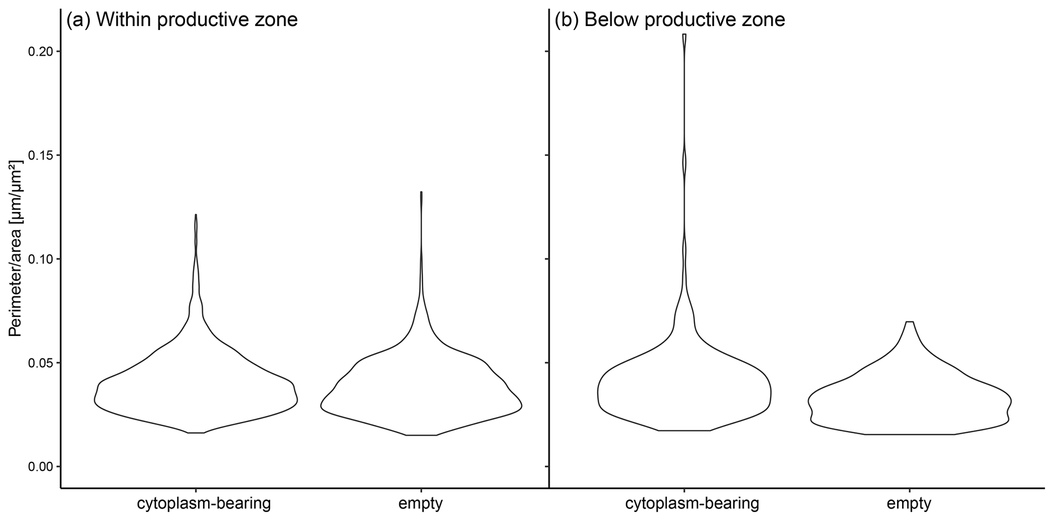
Figure A2The ratio of perimeter to area in individual shells of N. pachyderma in samples from PS 93.1 divided by the status (cytoplasm-bearing and empty). Panel (a) represents the shells from within the calculated productive zone of the individual stations and (b) those from below the productive zone.
Figure A3Change in mass flux between the net directly below the calculated base of the productive zone and the deepest net of sampling of each station divided by the different regions of sampling.
All data created for this study, including calculations made on published data, are available on PANGEA (https://doi.pangaea.de/10.1594/PANGAEA.941250, Tell, 2022). The data sources of abundances from published data are also listed in Table 1, and shell weights from the M39/4 expedition are listed as PANGEA references.
The study was designed by all authors. FT carried out the laboratory work with help from JM and the data analysis with help from LJ. All authors contributed to the interpretation and discussion of the results. FT wrote the paper with contributions from MK, LJ and JM.
The contact author has declared that none of the authors has any competing interests.
Publisher’s note: Copernicus Publications remains neutral with regard to jurisdictional claims in published maps and institutional affiliations.
The master and crew of R/V Polarstern and R/V Maria S. Merian are gratefully acknowledged for support of the work during the PS93, MSM44 and MSM66 cruises. We are very grateful to Birgit Lübben for conducting the size measurements on the MSM44 and MSM66 samples. We want to thank Mattia Greco for helping with access to samples and data. We further appreciate that Kirstin Werner gave us the possibility to work on the PS93.1 samples.
This research has been supported by the Deutsche Forschungsgemeinschaft (DFG) through the International Research Training Group “Processes and
impacts of climate change in the North Atlantic Ocean and the Canadian
Arctic” (grant no. IRTG 1904).
The article processing charges for this open-access publication were covered by the University of Bremen.
This paper was edited by Carolin Löscher and reviewed by Robert F. Spielhagen and Ralf Schiebel.
Amante, C. and Eakins, B. W.: ETOPO1 1 Arc-Minute Global Relief Model: Procedures, Data Sources and Analysis, NOAA Technical Memorandum NESDIS NGDC-24, National Geophysical Data Center, NOAA [data set], https://doi.org/10.7289/V5C8276M, 2009.
Anglada-Ortiz, G., Zamelczyk, K., Meilland, J., Ziveri, P., Chierici, M., Fransson, A., and Rasmussen, T. L.: Planktic Foraminiferal and Pteropod Contributions to Carbon Dynamics in the Arctic Ocean (North Svalbard Margin), Front. Mar. Sci., 8, 661158, https://doi.org/10.3389/fmars.2021.661158, 2021.
Arikawa, R.: Distribution and taxonomy of globigerina pachyderma (Ehrenberg) off the Sanriku coast, northeast Honshu, Japan, Tohoku Uiv., Sci. Rep., 2nd series (Geol.), 53, 103–157, 1983.
Bauch, D., Carstens, J., and Wefer, G.: Oxygen isotope composition of living Neogloboquadrina pachyderma (sin.) in the Arctic Ocean, Earth Planet. Sc. Lett., 146, 47–58, https://doi.org/10.1016/S0012-821X(96)00211-7, 1997.
Bauerfeind, E., Nöthig, E.-M., Beszczynska, A., Fahl, K., Kaleschke, L., Kreker, K., Klages, M., Soltwedel, T., Lorenzen, C., and Wegner, J.: Particle sedimentation patterns in the eastern Fram Strait during 2000–2005: Results from the Arctic long-term observatory HAUSGARTEN, Deep-Sea Res. Pt. I, 56, 1471–1487, https://doi.org/10.1016/j.dsr.2009.04.011, 2009.
Bauerfeind, E., Nöthig, E.-M., Pauls, B., Kraft, A., and Beszczynska-Möller, A.: Variability in pteropod sedimentation and corresponding aragonite flux at the Arctic deep-sea long-term observatory HAUSGARTEN in the eastern Fram Strait from 2000 to 2009, J. Mar. Syst., 132, 95–105, https://doi.org/10.1016/j.jmarsys.2013.12.006, 2014.
Baumann, K.-H., Andruleit, H., and Samtleben, C.: Coccolithophores in the Nordic Seas: comparison of living communities with surface sediment assemblages, Deep-Sea Res. Pt. II, 47, 1743–1772, https://doi.org/10.1016/S0967-0645(00)00005-9, 2000.
Bé, A. W.: Some observations on Arctic planktonic foraminifera, Contrib. Cushman Found, Foraminiferal Res., 11, 64–68, 1960.
Beaugrand, G., McQuatters-Gollop, A., Edwards, M., and Goberville, E.: Long-term responses of North Atlantic calcifying plankton to climate change, Nat. Clim. Change, 3, 263–267, https://doi.org/10.1038/nclimate1753, 2013.
Busch, K., Bauerfeind, E., and Nöthig, E.-M.: Pteropod sedimentation patterns in different water depths observed with moored sediment traps over a 4-year period at the LTER station HAUSGARTEN in eastern Fram Strait, Polar Biol., 38, 845–859, https://doi.org/10.1007/s00300-015-1644-9, 2015.
Carstens, J. and Wefer, G.: Recent distribution of planktonic foraminifera in the Nansen Basin, Arctic Ocean, Deep-Sea Res. Pt. A, 39, 507–524, https://doi.org/10.1016/S0198-0149(06)80018-X, 1992.
Carstens, J., Hebbeln, D., and Wefer, G.: Distribution of planktic foraminifera at the ice margin in the Arctic (Fram Strait), Mar. Micropaleontol., 29, 257–269, https://doi.org/10.1016/S0377-8398(96)00014-X, 1997.
Daniels, C., Poulton, A., Young, J., Esposito, M., Humphreys, M., Ribas-Ribas, M., Tynan, E., and Tyrrell, T.: Species-specific calcite production reveals Coccolithus pelagicus as the key calcifier in the Arctic Ocean, Mar. Ecol. Prog. Ser., 555, 29–47, https://doi.org/10.3354/meps11820, 2016.
Fahl, K. and Nöthig, E.-M.: Lithogenic and biogenic particle fluxes on the Lomonosov Ridge (central Arctic Ocean) and their relevance for sediment accumulation: Vertical vs. lateral transport, Deep-Sea Res. Pt. I, 54, 1256–1272, https://doi.org/10.1016/j.dsr.2007.04.014, 2007.
Field, D. B., Baumgartner, T. R., Charles, C. D., Ferreira-Bartrina, V., and Ohman, M. D.: Planktonic Foraminifera of the California Current Reflect 20th-Century Warming, Science, 311, 63–66, https://doi.org/10.1126/science.1116220, 2006.
Friedlingstein, P., Jones, M. W., O'Sullivan, M., Andrew, R. M., Hauck, J., Peters, G. P., Peters, W., Pongratz, J., Sitch, S., Le Quéré, C., Bakker, D. C. E., Canadell, J. G., Ciais, P., Jackson, R. B., Anthoni, P., Barbero, L., Bastos, A., Bastrikov, V., Becker, M., Bopp, L., Buitenhuis, E., Chandra, N., Chevallier, F., Chini, L. P., Currie, K. I., Feely, R. A., Gehlen, M., Gilfillan, D., Gkritzalis, T., Goll, D. S., Gruber, N., Gutekunst, S., Harris, I., Haverd, V., Houghton, R. A., Hurtt, G., Ilyina, T., Jain, A. K., Joetzjer, E., Kaplan, J. O., Kato, E., Klein Goldewijk, K., Korsbakken, J. I., Landschützer, P., Lauvset, S. K., Lefèvre, N., Lenton, A., Lienert, S., Lombardozzi, D., Marland, G., McGuire, P. C., Melton, J. R., Metzl, N., Munro, D. R., Nabel, J. E. M. S., Nakaoka, S.-I., Neill, C., Omar, A. M., Ono, T., Peregon, A., Pierrot, D., Poulter, B., Rehder, G., Resplandy, L., Robertson, E., Rödenbeck, C., Séférian, R., Schwinger, J., Smith, N., Tans, P. P., Tian, H., Tilbrook, B., Tubiello, F. N., van der Werf, G. R., Wiltshire, A. J., and Zaehle, S.: Global Carbon Budget 2019, Earth Syst. Sci. Data, 11, 1783–1838, https://doi.org/10.5194/essd-11-1783-2019, 2019.
Greco, M., Jonkers, L., Kretschmer, K., Bijma, J., and Kucera, M.: Depth habitat of the planktonic foraminifera Neogloboquadrina pachyderma in the northern high latitudes explained by sea-ice and chlorophyll concentrations, Biogeosciences, 16, 3425–3437, https://doi.org/10.5194/bg-16-3425-2019, 2019.
Greco, M., Morard, R., and Kucera, M.: Single-cell metabarcoding reveals biotic interactions of the Arctic calcifier Neogloboquadrina pachyderma with the eukaryotic pelagic community, J. Plank. Res., 43, 113–125, https://doi.org/10.1093/plankt/fbab015, 2021a.
Greco, M., Werner, K., Zamelczyk, K., Rasmussen, T. L., and Kucera, M.: Decadal trend of plankton community change and habitat shoaling in the Arctic gateway recorded by planktonic foraminifera, Glob. Change Biol., 28, 1798–1808, https://doi.org/10.1111/gcb.16037, 2021b.
Hebbeln, D.: Flux of ice-rafted detritus from sea ice in the Fram Strait, Deep-Sea Res. Pt. II, 47, 1773–1790, https://doi.org/10.1016/S0967-0645(00)00006-0, 2000.
Hemleben, C., Spindler, M., and Anderson, O. R.: Modern planktonic foraminifera, Springer Science & Business Media, ISBN 1-4612-3544-8, 1989.
Henehan, M. J., Evans, D., Shankle, M., Burke, J. E., Foster, G. L., Anagnostou, E., Chalk, T. B., Stewart, J. A., Alt, C. H., and Durrant, J.: Size-dependent response of foraminiferal calcification to seawater carbonate chemistry, Biogeosciences, 14, 3287–3308, https://doi.org/10.5194/bg-14-3287-2017, 2017.
Jensen, S.: Planktische Foraminiferen im Europäischen Nordmeer: Verbreitung und Vertikalfluss sowie ihre Entwicklung während der letzten 15000 Jahre, Ph.D. thesis, Christian-Albrechts-Universität Kiel, Kiel, Germany, Berichte aus dem Sonderforschungsbereich 313, Veränderungen der Umwelt – Der Nördliche Nordatlantik, 75, 105 pp., 1998.
Jonkers, L., Brummer, G.-J. A., Peeters, F. J. C., van Aken, H. M., and De Jong, M. F.: Seasonal stratification, shell flux, and oxygen isotope dynamics of left-coiling N. pachyderma and T. quinqueloba in the western subpolar North Atlantic, Paleoceanography, 25, PA2204, https://doi.org/10.1029/2009PA001849, 2010.
Jonkers, L., Hillebrand, H., and Kucera, M.: Global change drives modern plankton communities away from the pre-industrial state, Nature, 570, 372–375, https://doi.org/10.1038/s41586-019-1230-3, 2019.
Jutterström, S. and Anderson, L. G.: The saturation of calcite and aragonite in the Arctic Ocean, Mar. Chem., 94, 101–110, https://doi.org/10.1016/j.marchem.2004.08.010, 2005.
Kiss, P., Jonkers, L., Hudáčková, N., Reuter, R. T., Donner, B., Fischer, G., and Kučera, M.: Determinants of Planktonic Foraminifera Calcite Flux: Implications for the Prediction of Intra-and Interannual Pelagic Carbonate Budgets, Global Biogeochem. Cy., 35, 9, https://doi.org/10.1029/2020GB006748, 2021.
Klaas, C. and Archer, D. E.: Association of sinking organic matter with various types of mineral ballast in the deep sea: Implications for the rain ratio, Ocean Carbon-Mineral Flux Association, Global Biogeochem. Cy., 16, 63-1–63-14, https://doi.org/10.1029/2001GB001765, 2002.
Kohfeld, K. E.: Geochemistry and ecology of polar planktonic foraminifera, and applications to paleoceanographic reconstructions, Ph.D. thesis, Columbia University, UnitedStates, 250 pp., 1998.
Kohfeld, K. E., Fairbanks, R. G., Smith, S. L., and Walsh, I. D.: Neogloboquadrina pachyderma (sinistral coiling) as paleoceanographic tracers in polar oceans: Evidence from Northeast Water Polynya plankton tows, sediment traps, and surface sediments, Paleoceanography, 11, 679–699, https://doi.org/10.1029/96PA02617, 1996.
Lončarić, N., Peeters, F. J. C., Kroon, D., and Brummer, G.-J. A.: Oxygen isotope ecology of recent planktic foraminifera at the central Walvis Ridge (SE Atlantic), Palaeoceanography, 21, PA3009, https://doi.org/10.1029/2005PA001207, 2006.
Manno, C. and Pavlov, A. K.: Living planktonic foraminifera in the Fram Strait (Arctic): absence of diel vertical migration during the midnight sun, Hydrobiologia, 721, 285–295, https://doi.org/10.1007/s10750-013-1669-4, 2014.
Meilland, J., Siccha, M., Weinkauf, M. F. G., Jonkers, L., Morard, R., Baranowski, U., Baumeister, A., Bertlich, J., Brummer, G.-J., Debray, P., Fritz-Endres, T., Groeneveld, J., Magerl, L., Munz, P., Rillo, M. C., Schmidt, C., Takagi, H., Theara, G., and Kucera, M.: Highly replicated sampling reveals no diurnal vertical migration but stable species-specific vertical habitats in planktonic foraminifera, J. Plank. Res., 41, 127–141, https://doi.org/10.1093/plankt/fbz002, 2019.
Meilland, J., Howa, H., Hulot, V., Demangel, I., Salaün, J., and Garlan, T.: Population dynamics of modern planktonic foraminifera in the western Barents Sea, Biogeosciences, 17, 1437–1450, https://doi.org/10.5194/bg-17-1437-2020, 2020.
Meilland, J., Siccha, M., Kaffenberger, M., Bijma, J., and Kucera, M.: Population dynamics and reproduction strategies of planktonic foraminifera in the open ocean, Biogeosciences, 20, 5789–5809, https://doi.org/10.5194/bg-2021-141, 2021.
Miller, L. A., Macdonald, R. W., McLaughlin, F., Mucci, A., Yamamoto-Kawai, M., Giesbrecht, K. E., and Williams, W. J.: Changes in the marine carbonate system of the western Arctic: patterns in a rescued data set, Polar Res., 33, 20577, https://doi.org/10.3402/polar.v33.20577, 2014.
Ofstad, S., Meilland, J., Zamelczyk, K., Chierici, M., Fransson, A., Gründger, F., and Rasmussen, T. L.: Development, productivity and seasonality of living planktonic foraminiferal faunas and Limacina helicina in an area of intense methane seepage in the Barents Sea, J. Geophys. Res.-Biogeo., 125, 2, https://doi.org/10.1029/2019JG005387, 2020.
Pados, T. and Spielhagen, R. F.: Species distribution and depth habitat of recent planktic foraminifera in Fram Strait, Arctic Ocean, Polar Res., 33, 22483, https://doi.org/10.3402/polar.v33.22483, 2014.
Pados, T., Spielhagen, R. F., Bauch, D., Meyer, H., and Segl, M.: Oxygen and carbon isotope composition of modern planktic foraminifera and near-surface waters in the Fram Strait (Arctic Ocean) – a case study, Biogeosciences, 12, 1733–1752, https://doi.org/10.5194/bg-12-1733-2015, 2015.
Peeters, F. J. C. and Brummer, G.-J. A.: The seasonal and vertical distribution of living planktic foraminifera in the NW Arabian Sea, Geol. Soc. Lond. Special Publ., 195, 463–497, https://doi.org/10.1144/GSL.SP.2002.195.01.26, 2002.
R Core Team: R: A Language and Environment for Statistical Computing, https://www.r-project.org (last access: 15 April 2022), 2018.
Riebesell, U., Kortzinger, A., and Oschlies, A.: Sensitivities of marine carbon fluxes to ocean change, P. Natl. Acad. Sci. USA, 106, 20602–20609, https://doi.org/10.1073/pnas.0813291106, 2009.
Salmon, K. H., Anand, P., Sexton, P. F., and Conte, M.: Upper ocean mixing controls the seasonality of planktonic foraminifer fluxes and associated strength of the carbonate pump in the oligotrophic North Atlantic, Biogeosciences, 12, 223–235, https://doi.org/10.5194/bg-12-223-2015, 2015.
Salter, I., Schiebel, R., Ziveri, P., Movellan, A., Lampitt, R., and Wolff, G. A.: Carbonate counter pump stimulated by natural iron fertilization in the Polar Frontal Zone, Nat. Geosci., 7, 885–889, https://doi.org/10.1038/ngeo2285, 2014.
Schiebel, R.: Planktic foraminiferal sedimentation and the marine calcite budget, Global Biogeochem. Cy., 16, 3-1–3-21, https://doi.org/10.1029/2001GB001459, 2002.
Schiebel, R. and Hemleben, C.: Interannual variability of planktic foraminiferal populations and test flux in the eastern North Atlantic Ocean (JGOFS), Deep-Sea Res. Pt. II, 47, 1809–1852, https://doi.org/10.1016/S0967-0645(00)00008-4, 2000.
Schiebel, R., Hiller, B., and Hemleben, C.: Impacts of storms on recent planktic foraminiferal test production and CaCO3 flux in the North Atlantic at 47∘ N, 20∘ W (JGOFS), Mar. Micropaleontol., 26, 115–129, https://doi.org/10.1016/0377-8398(95)00035-6, 1995.
Schiebel, R., Barker, S., Lendt, R., Thomas, H., and Bollmann, J.: Planktic foraminiferal dissolution in the twilight zone, Deep-Sea Res. Pt. II, 54, 676–686, https://doi.org/10.1016/j.dsr2.2007.01.009, 2007.
Schiebel, R., Spielhagen, R. F., Garnier, J., Hagemann, J., Howa, H., Jentzen, A., Martínez-Garcia, A., Meilland, J., Michel, E., Repschläger, J., Salter, I., Yamasaki, M., and Haug, G.: Modern planktic foraminifers in the high-latitude ocean, Mar. Micropaleontol., 136, 1–13, https://doi.org/10.1016/j.marmicro.2017.08.004, 2017.
Schiebel, R., Smart, S. M., Jentzen, A., Jonkers, L., Morard, R., Meilland, J., Michel, E., Coxall, H. K., Hull, P. M., de Garidel-Thoron, T., Aze, T., Quillévéré, F., Ren, H., Sigman, D. M., Vonhof, H. B., Martínez-García, A., Kučera, M., Bijma, J., Spero, H. J., and Haug, G. H.: Advances in planktonic foraminifer research: New perspectives for paleoceanography, Revue Micropaléontol., 61, 113–138, https://doi.org/10.1016/j.revmic.2018.10.001, 2018.
Schönfeld, J., Golikova, E., Korsun, S., and Spezzaferri, S.: The Helgoland Experiment – assessing the influence of methodologies on Recent benthic foraminiferal assemblage composition, J. Micropalaeontol., 32, 161–182, https://doi.org/10.1144/jmpaleo2012-022, 2013.
Siccha, M. and Kucera, M.: ForCenS, a curated database of planktonic foraminifera census counts in marine surface sediment samples, Sci. Data, 4, 170109, https://doi.org/10.1038/sdata.2017.109, 2017.
Siccha, M., Schiebel, R., Schmidt, S., and Howa, H.: Short-term and small-scale variability in planktic foraminifera test flux in the Bay of Biscay, Deep-Sea Res. Pt. I, 64, 146–156, https://doi.org/10.1016/j.dsr.2012.02.004, 2012.
Simstich, J.: Die ozeanische Deckschicht des Europäischen Nordmeers im Abbild stabiler Isotope von Kalkgehäusen unterschiedlicher Planktonforaminiferenarten, Ph.D. thesis, Berichte – Reports 2, Institut für Geowissenschaften, Christian-Albrechts-Universität, Kiel, Germany, 96 pp., 1999.
Simstich, J., Sarnthein, M., and Erlenkeuser, H.: Paired δ18O signals of Neogloboquadrina pachyderma (s) and Turborotalita quinqueloba show thermal stratification structure in Nordic Seas, Mar. Micropaleontol., 48, 107–125, https://doi.org/10.1016/S0377-8398(02)00165-2, 2003.
Soltwedel, T., Bauerfeind, E., Bergmann, M., Budaeva, N., Hoste, E., Jaeckisch, N., von Juterzenka, K., Matthießen, J., Mokievsky, V., and Nöthig, E.-M.: HAUSGARTEN: multidisciplinary investigations at a deep-sea, long-term observatory in the Arctic Ocean, Oceanography, 18, 46–61, https://doi.org/10.5670/oceanog.2005.24, 2005.
Spindler, M.: On the salinity tolerance of the planktonic foraminifer Neogloboquadrina pachyderma from Antarctic sea ice, Proc. NIPR Symp., Polar Biol., 9, 85–91, 1996.
Stangeew, E.: Distribution and Isotopic Composition of Living Planktonic Foraminifera N. pachyderma (sinistral) and T. quinqueloba in the High Latitude North Atlantic, PhD Thesis, Christian-Albrechts Universität zu Kiel, Germany, 90 pp., M39/4_361CTD-18, https://doi.pangaea.de/10.1594/PANGAEA.62182, M39/4_402CTD-55, https://doi.pangaea.de/10.1594/PANGAEA.62183, 2001.
Steinacher, M., Joos, F., Frölicher, T. L., Plattner, G.-K., and Doney, S. C.: Imminent ocean acidification in the Arctic projected with the NCAR global coupled carbon cycle-climate model, Biogeosciences, 6, 515–533, https://doi.org/10.5194/bg-6-515-2009, 2009.
Sulpis, O., Jeansson, E., Dinauer, A., Lauvset, S. K., and Middelburg, J. J.: Calcium carbonate dissolution patterns in the ocean, Nat. Geosci., 14, 423–428, https://doi.org/10.1038/s41561-021-00743-y, 2021.
Takahashi, K. and Bé, A. W. H.: Planktonic foraminifera: factors controlling sinking speeds, Deep-Sea Res. Pt. A, 31, 1477–1500, https://doi.org/10.1016/0198-0149(84)90083-9, 1984.
Tell, F.: Neogloboquadrina pachyderma compiled data from vertical profiles in the Arctic Ocean, PANGAEA [data set], https://doi.pangaea.de/10.1594/PANGAEA.941250, last access: 15 February 2022.
Vihtakari, M.: ggOceanMaps: Plot Data on Oceanographic Maps using “ggplot2”, R package version 1.1.19, Zenodo [code], https://doi.org/10.5281/zenodo.4554714, 2021 (available at: https://github.com/MikkoVihtakari/ggOceanMaps, last access: 15 February 2022).
Vilks, G.: Comparison of Globorotalia pachyderma (Ehrenberg) in the water column and sediments of the Canadian Arctic, J. Foramin. Res., 5, 313–325, https://doi.org/10.2113/gsjfr.5.4.313, 1975.
Volkmann, R.: Planktic foraminifer ecology and stable isotope geochemistry in the Arctic Ocean: implications from water column and sediment surface studies for quantitative reconstructions of oceanic parameters, Ph. D. thesis, Berichte zur Polarforschung (Reports on Polar Research), 361, Alfred-Wegener-Institute, Bremerhaven, Germany, 100 pp., https://doi.org/10.2312/BzP_0361_2000, 2000a.
Volkmann, R.: Planktic foraminifers in the outer Laptev Sea and the Fram Strait – modern distribution and ecology, J. Foramin. Res., 30, 157–176, https://doi.org/10.2113/0300157, 2000b.
Volkmann, R. and Mensch, M.: Stable isotope composition (δ18O, δ13C) of living planktic foraminifers in the outer Laptev Sea and the Fram Strait, Mar. Micropaleontol., 26, 163–188, https://doi.org/10.1016/S0377-8398(01)00018-4, 2001.
von Bodungen, B., Antia, A., Bauerfeind, E., Haupt, O., Koeve, W., Machado, E., Peeken, I., Peinert, R., Reitmeier, S., Thomsen, C., Voss, M., Wunsch, M., Zeller, U., and Zeitzschel, B.: Pelagic processes and vertical flux of particles: an overview of a long-term comparative study in the Norwegian Sea and Greenland Sea, Geol. Rundsch., 84, 11–27, https://doi.org/10.1007/BF00192239, 1995.
von Gyldenfeldt, A.-B., Carstens, J., and Meincke, J.: Estimation of the catchment area of a sediment trap by means of current meters and foraminiferal tests, Deep-Sea Res. Pt. II, 47, 1701–1717, https://doi.org/10.1016/S0967-0645(00)00004-7, 2000.
Wassmann, P., Kosobokova, K. N., Slagstad, D., Drinkwater, K. F., Hopcroft, R. R., Moore, S. E., Ellingsen, I., Nelson, R. J., Carmack, E., Popova, E., and Berge, J.: The contiguous domains of Arctic Ocean advection: Trails of life and death, Prog. Oceanogr., 139, 42–65, https://doi.org/10.1016/j.pocean.2015.06.011, 2015.
Weinkauf, M. F. G., Kunze, J. G., Waniek, J. J., and Kučera, M.: Seasonal Variation in Shell Calcification of Planktonic Foraminifera in the NE Atlantic Reveals Species-Specific Response to Temperature, Productivity, and Optimum Growth Conditions, PLOS ONE, 33, 11, https://doi.org/10.1371/journal.pone.0148363, 2016.
Wolfteich, C. M.: Satellite-derived sea surface temperature, mesoscale variability, and foraminiferal production in the North Atlantic, M.S. thesis, Massachusetts Institute of Technology and Woods Hole Oceanographic Institution, Woods Hole, Massachusetts, USA, https://doi.org/10.1575/1912/5556, 1994.
Zeebe, R. E.: History of Seawater Carbonate Chemistry, Atmospheric CO2, and Ocean Acidification, Annu. Rev. Earth Planet. Sci., 40, 141–165, https://doi.org/10.1146/annurev-earth-042711-105521, 2012.