the Creative Commons Attribution 4.0 License.
the Creative Commons Attribution 4.0 License.
 | 10 Nov 2022
Management-induced changes in soil organic carbon on global croplands
Kristine Karstens
Benjamin Leon Bodirsky
Jan Philipp Dietrich
Marta Dondini
Jens Heinke
Matthias Kuhnert
Christoph Müller
Susanne Rolinski
Pete Smith
Isabelle Weindl
Hermann Lotze-Campen
Alexander Popp
Soil organic carbon (SOC), one of the largest terrestrial carbon (C) stocks on Earth, has been depleted by anthropogenic land cover change and agricultural management. However, the latter has so far not been well represented in global C stock assessments. While SOC models often simulate detailed biochemical processes that lead to the accumulation and decay of SOC, the management decisions driving these biophysical processes are still little investigated at the global scale. Here we develop a spatially explicit data set for agricultural management on cropland, considering crop production levels, residue returning rates, manure application, and the adoption of irrigation and tillage practices. We combine it with a reduced-complexity model based on the Intergovernmental Panel on Climate Change (IPCC) tier 2 method to create a half-degree resolution data set of SOC stocks and SOC stock changes for the first 30 cm of mineral soils. We estimate that, due to arable farming, soils have lost around 34.6 GtC relative to a counterfactual hypothetical natural state in 1975. Within the period 1975–2010, this SOC debt continued to expand by 5 GtC (0.14 GtC yr−1) to around 39.6 GtC. However, accounting for historical management led to 2.1 GtC fewer (0.06 GtC yr−1) emissions than under the assumption of constant management. We also find that management decisions have influenced the historical SOC trajectory most strongly by residue returning, indicating that SOC enhancement by biomass retention may be a promising negative emissions technique. The reduced-complexity SOC model may allow us to simulate management-induced SOC enhancement – also within computationally demanding integrated (land use) assessment modeling.
- Article
(6386 KB) - Full-text XML
- BibTeX
- EndNote


Soil organic carbon (SOC), the amount of organic carbon stored in the Earth's soil, exceeds the carbon in the atmospheric and vegetation pools by multiple times (Batjes, 1996). Even small changes in processes affecting SOC lead, therefore, to substantial shifts in the terrestrial carbon cycle and influence the amount of CO2 in the atmosphere (Friedlingstein et al., 2020; Minasny et al., 2017). The specific amount of carbon stored in soils globally is quantified with estimates ranging from 1500 to 2400 GtC for the first meter of the soil profile (Batjes, 1996; Sanderman et al., 2017).
Natural properties like climatic, biophysical, and landscape characteristics clearly play the most important roles in determining SOC variations over space and time. Recent studies have focused on the evaluation of total SOC stocks of the world and on the spatial disaggregation of soil properties such as SOC content (Batjes, 2016; Hengl et al., 2017; FAO, 2019). However, these studies often do not include human intervention, like land cover change and agricultural management, in their analysis. Compared to climatic and geological driving forces, human interventions alter terrestrial carbon pools over much shorter timescales and are currently one of the most dominant drivers of SOC changes on managed land (Hansis et al., 2015; Bastos et al., 2021).
The anthropogenic impact can be measured by the SOC debt (also referred to as the SOC component of land use change emissions; see Pongratz et al., 2014), which is the amount of organic carbon soils have lost under cultivation compared to a hypothetical potential natural vegetation state. Sanderman et al. (2017) identified the anthropogenic SOC debt for the first meter of the soil profile due to land cover change at around 116 GtC (37 GtC for the first 30 cm), compared to previous estimates of 60–130 GtC for the first meter (Lal, 2001).
Global assessments of the carbon cycle via dynamic global vegetation models (DGVMs), Earth system models (ESMs), or bookkeeping models (BKMs) have analyzed SOC losses as part of a comprehensive evaluation of the global carbon budget and land use change (LUC) emissions (Friedlingstein et al., 2020). While providing estimates of the magnitude of SOC losses due to land cover change, most models lack a detailed representation of agricultural management. Earlier DGVM- and ESM-based assessments only considered changes in land cover but ignored the removal of biomass at harvest (Strassmann et al., 2008; Betts et al., 2015). BKMs are designed to estimate LUC-related emissions and have largely been improved in the estimation of additional emissions from wood harvest and shifting cultivation. However, state-of-the-art models do not consider impacts of varying agricultural management (Friedlingstein et al., 2020; Houghton et al., 2012; Hansis et al., 2015; Bastos et al., 2021).
Managed agricultural systems were introduced in greater detail to DGVMs and ESMs to improve the assessment of the terrestrial carbon balance (e.g., Bondeau et al., 2007; Lindeskog et al., 2013). Pugh et al. (2015) explicitly consider agricultural management in the form of tillage, irrigation, and biomass extraction at harvest but worked with uniform scenario assumptions on management rather than with historical management data. They also showed the importance of accounting for the land use history, as many carbon emissions from agricultural soils are caused by historical LUC and the slow decline of SOC under cropland before a new equilibrium is reached.
In global-scale carbon cycle assessments, management systems are typically represented as spatially explicit patterns that are static in time (e.g., for growing seasons in Portmann et al., 2010, multiple cropping systems in Waha et al., 2020, and irrigation systems in Jägermeyr et al., 2015) or as stylized (in the sense of uniform management assumptions) scenarios (e.g., Pugh et al., 2015; Lutz et al., 2019). Herzfeld et al. (2021) account for historical changes in fertilizer and manure inputs, residue removal rates, and tillage systems and report SOC losses from cropland expansion over the period from 1700–2018 of 215 GtC. Within their stylized future management scenarios under future climate change, they find that none of the management aspects considered (residue management and no tillage) can create a positive SOC stock change on current cropland areas that counteracts the still-continuing legacy flux from the initial land use change.
More data sets on spatially explicit agricultural management time series with global coverage are becoming available (e.g., on tillage systems; see Porwollik et al., 2019 and Prestele et al., 2018), and modeling approaches are increasingly being developed to project the dynamics of management systems into the future (e.g., Iizumi et al., 2019; Minoli et al., 2019), but have – to our knowledge – not yet found their way into comprehensive assessments of the terrestrial carbon cycle in DGVMs and BKMs.
Field-scale models (Del Grosso et al., 2001; Coleman et al., 1997; Smith et al., 2010; Taghizadeh-Toosi et al., 2014) are able to better account for historical agricultural management if detailed information on crop yield levels, fertilizer inputs, and various other on-farm measures are available for the studied sites. However, due to the lack of comprehensive global management data as input to these models, scaling up to the global domain remains a complex challenge (Morais et al., 2019).
Managed soils have been increasingly studied not only for their carbon emitting behavior but also because of their capacity to restore carbon (soil carbon sequestration (SCS) techniques). However, assessing SCS dynamically, considering the interdependency with environmental, social, and economic sustainability targets, has been difficult so far, as integrated assessment models (IAMs; Popp et al., 2016; Rogelj et al., 2018; Forster et al., 2018) have not integrated soil management into their mitigation pathways. More detailed process-based models are typically computationally too demanding to be integrated into optimization-based IAMs. Better accounting for soil carbon management in IAMs thus requires a lightweight model suitable for iterative modeling with detailed options to represent agricultural soil management.
The objectives of our study are (1) to develop a reduced-complexity SOC model able to account for SCS in IAM frameworks, (2) to create a comprehensive data set of the global gridded management time series, including crop production levels, residue input rates, manure amendments, and the adoption of irrigation and tillage practices, and (3) to provide global and spatially explicit SOC and SOC debt estimates that consider spatially explicit and time-variant agricultural management. We decompose the contribution of different management activities through a scenario analysis, identifying the management decisions impacting SOC development the most. Moreover, we compare our model performance against other SOC stock and SOC emission estimates to evaluate the suitability of this reduced-complexity approach for integration into IAM modeling.
In Sect. 2.1, we introduce the basic concept of SOC dynamics as applied in this study and explained in more detail in the refinement of the Intergovernmental Panel on Climate Change (IPCC) guidelines vol. 4, chap. 5 on “Cropland” (IPCC, 2019). We additionally describe how we configured and extended the tier 2 modeling approach (for the model code, see Karstens and Dietrich, 2022). In Sect. 2.2, we briefly refer to the concept of stock change factors, as outlined in the tier 1 approach of the IPCC guidelines (IPCC, 2006, 2019). Section 2.3 provides a detailed description of the global, gridded management data used to drive the model, including crop production levels, residue input rates, manure amendments, and the adoption of irrigation and tillage practices (for the model code, see Bodirsky et al., 2022a). In Sect. 2.4, we define the management scenarios used to analyze the role of different management aspects in historical cropland SOC dynamics.
2.1 SOC stocks and stock changes following the tier 2 modeling approach
Following the tier 2 modeling approach of the refinement of the IPCC guidelines vol. 4, chap. 5 on “Cropland” (IPCC, 2019), which is referred to as the tier 2 modeling approach in the following, we estimate SOC stocks and their change over time for cropland at a half-degree resolution from 1975 to 2010. We restrict our analysis to the first 0–30 cm of the soil profile. Moreover, we assume the current SOC state converges towards a steady state, which itself depends on biophysical, climatic, and agronomic conditions. Therefore, we take the following three steps for each year of our simulation period:
-
We calculate annual land-use-type-specific steady states and decay rates for SOC stocks (Sect. 2.1.1).
-
We account for land conversion by transferring SOC from and to natural vegetation (Sect. 2.1.2).
-
We estimate SOC stocks and changes based on the stocks of the previous time step, the steady-state stocks, and the decay rate (Sect. 2.1.3).
To initialize the first year of our simulation period, we use a spin-up period of 465 years (Sect. 2.1.4).
2.1.1 Steady-state SOC stocks and decay rates
In a simple first-order kinetic approach, the steady-state soil organic carbon stocks SOCeq are given by the following:
with Cin being the carbon inputs to the soil, and k denotes the soil organic carbon decay rate. This equation is valid for all grid cells i and all years t. We use the tier 2 modeling approach for our calculations, which assumes three soil carbon sub-pools (sub; active, slow, and passive) and the interactions between them, following the approach in the CENTURY model (Parton et al., 1987). Annual carbon inflow to each sub-pool and annual decay rates of each sub-pool are land-use-type (lu) specific. We distinguish two land use types, i.e., cropland and uncropped land under potential natural vegetation as representative for all other land use types, including forestry and grasslands (referred to as natural vegetation in the following). Forage crops are included within cropland, whereas pastures (including mowed meadows (perennials) and rangelands) are assigned to natural vegetation. Carbon flows connected to livestock are only considered in this study when they originate from cropland feed sources, while the manure originating from pasture biomass is disregarded, implicitly assuming that this manure is excreted or applied to pastures.
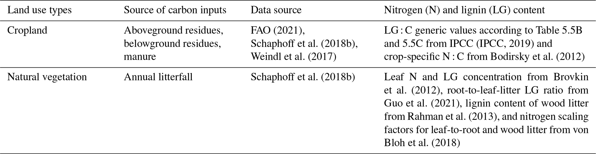
Carbon inputs for cropland are below- and aboveground crop residues left or returned to the field (see Sect. 2.3.2) and manure inputs (see Sect. 2.3.3); for natural vegetation, litterfall, including fine root turnover (Schaphoff et al., 2018b), is the only source of carbon inflow to the soil. Following the IPCC guidelines (IPCC, 2019, chap. 5), carbon inputs are disaggregated into metabolic and structural components, depending on their lignin and nitrogen content. For each component, the sum of all carbon input sources is allocated to the respective SOC sub-pools via transfer coefficients. This implies that both the amount of carbon and its structural composition determine the effective inflow into the different pools.
Whereas residue and manure default lignin and nitrogen fractions are given by the IPCC guidelines (IPCC, 2019, chap. 5), we use plant-functional-type and plant-organ-specific parameterization for the natural litterfall. The global distribution of plant functional types is given by Schaphoff et al. (2018b) and includes the separation of litter into leaf, fine root, and wood litter compartments, while excluding litter biomass burned in wild fires. Leaf litter parameters are given by Brovkin et al. (2012), the fine-root-to-leaf-litter lignin ratio by Guo et al. (2021), the lignin content of wood litter by Rahman et al. (2013), and the nitrogen content scaling factors for leaves to fine roots and leaf to wood litter by von Bloh et al. (2018). Data sources for all considered carbon inputs and for lignin and nitrogen parameterization are listed in Table 1.
FAO (2021)Schaphoff et al. (2018b)Weindl et al. (2017)(IPCC, 2019)Bodirsky et al. (2012)Schaphoff et al. (2018b)Brovkin et al. (2012)Guo et al. (2021)Rahman et al. (2013)von Bloh et al. (2018)Table 1Type and data sources for carbon inputs and parameterization to different land use types.
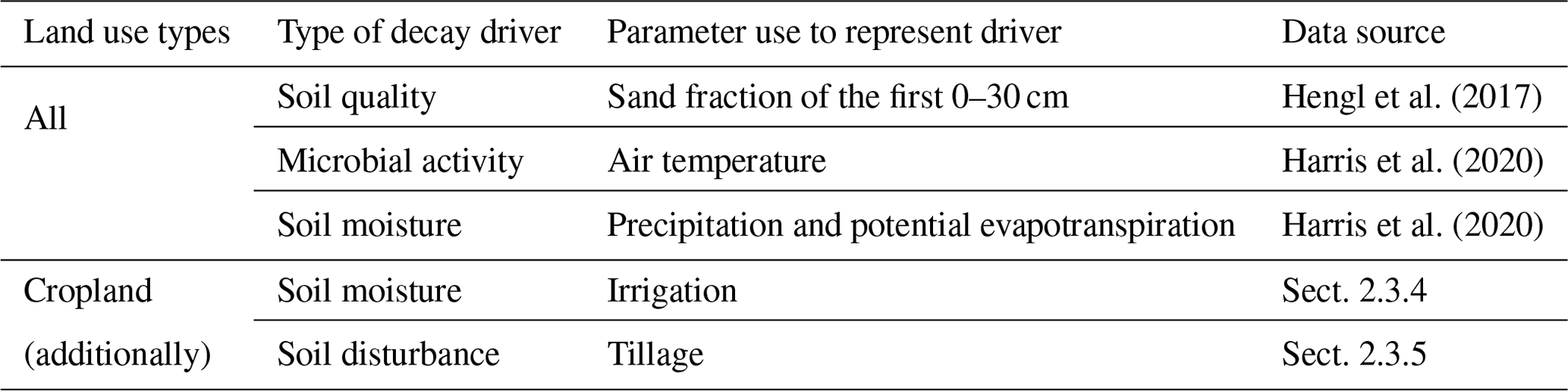
The sub-pool-specific decay rates ksub are influenced by climatic conditions, biophysical and biochemical soil properties, and management factors that all vary over space i and time t. Following the tier 2 modeling approach (IPCC, 2019, chap. 5), we consider temperature (temp), water (wat), sand fraction (sf), and tillage (till) effects to account for spatial and temporal variation in decay rates. Thus, ksub rates are given by the following:
For natural vegetation, we assume rainfed and non-tilled conditions, whereas for cropland, we distinguish the effect of different tillage (see Sect. 2.3.5) and irrigation (see Sect. 2.3.4) practices on decay rates. We calculate area-weighted means for till and wat on cropland for each grid cell, using area shares for the different tillage and irrigation practices. Data sources and used parameters for the different decay drivers for all land use types are listed in Table 2; equations are based on Eqs. (5.0B)–(5.0F) in IPCC (2019).
Hengl et al. (2017)Harris et al. (2020)Harris et al. (2020)Table 2Type and data sources for carbon inputs to different land use types.
2.1.2 SOC transfer between land use types
We calculate SOC stocks based on the area shares of land use types (lu) within our grid cells i. If land is converted from one land use type into the other , then a respective share of the SOC is reallocated within our budget. We do not distinguish between newly converted and existing cropland but can work with the average carbon content, as the relative decay of SOC is proportional to the SOC stock (see Fig. 1). We account for land conversion at the beginning of each time step t by calculating a preliminary stock SOC via the following:
with Alu being the land use type specific areas, ARlu the area reduction, and AElu the area expansion of the two land use types. Data sources and methodology on land use states and changes are described in Sect. 2.3.1.
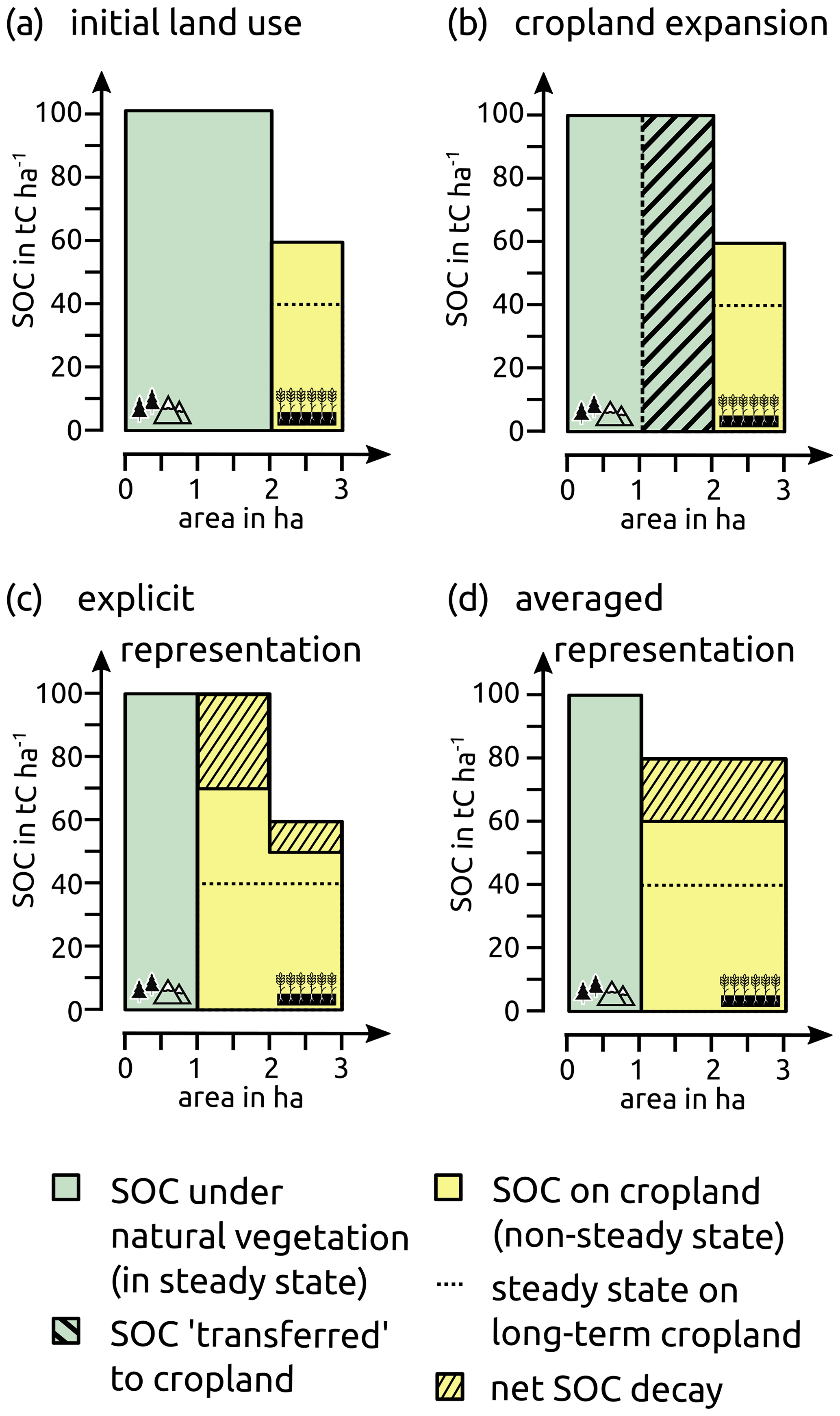
Figure 1Scheme of the land use transition representation. Given an initial land use pattern (as in this example, with 2 ha land under natural vegetation and 1 ha of cropland), there are separate SOC stocks for natural vegetation and cropland. While, in this example, we assume SOC under natural vegetation to be in a steady state, the cropland SOC stock approaches its steady state without having reached it yet (a). Upon cropland expansion (in this example, half of the natural vegetation is cleared to be used as cropland), SOC stocks on cropland increase due to a transfer of land from natural vegetation (b). Explicitly representing newly converted cropland and existing cropland to account for SOC dynamics (c) leads to the same weighted mean value as averaging SOC stocks (d), due to the linearity of Eq. 4 and cropland age-independent decay rates (see Eq. 2).
2.1.3 Total SOC stocks and stock changes
SOC converges towards the calculated steady-state stock SOCeq for each grid cell i, each annual time step t, each land use type lu, and each sub-pool sub, in the following:
Note that the decay rates have to be multiplied by 1 year (1 a) to form a dimensionless factor. Reformulating this equation, we obtain a mass balance equation as follows:
The global SOC stock for each time step t can then be calculated via the following:
According to the IPCC guidelines, SOC changes can be expressed as the difference of 2 consecutive years (see Eq. 5.0A in IPCC, 2019). This, however, will also include naturally occurring changes due to climatic variation over time. For our study, we define the absolute and relative SOC changes in relation to a potential natural-state SOCpnv under the same climatic conditions in grid cell i at time t that is based on the natural vegetation SOC calculations, as defined above, without accounting for land conversion from cropland at any time. The absolute changes ΔSOC and relative changes FSCF are thus given by the following:
Note that the absolute changes ΔSOC can also be interpreted as the SOC debt (Sanderman et al., 2017) due to human cropping activities, whereas relative changes FSCF can be considered to be stock change factors, as defined within the IPCC guidelines of 2006 (IPCC, 2006). Moreover, ΔSOC is equivalent to the negated cumulative SOC component of human land use change emissions (Pugh et al., 2015).
2.1.4 Initialization of SOC pools
The initialization of SOC pools is very important and has to include the proper accounting for the land use history, as many CO2 emissions from agricultural soils are caused by historical land use change (LUC) and the slow decline of SOC under crop cultivation before it reaches a new equilibrium. We initialize our SOC sub-pools using a three-step approach, since the input data availability is limited for climate and litter estimates (starting only in 1901) and for agricultural management data (starting only in 1965).
First, in order to account for the impacts of legacy fluxes from land use changes long before the time horizon of interest, we consider land use change from 1510 onwards. In 1510, we assume all SOC pools to be in natural steady state, implying that all land use change prior to that time occurs in 1510. We assume that, by 1901, all cropland converted in 1510 has reached its new steady state, so that it is not necessary to explicitly account for even older land conversion. Model inputs for 1901–1930 for climate and natural vegetation litterfall are repeated for 1510–1900 to mimic constant climate conditions for this first initializing period. Similarly, agricultural management data are held constant at the level of 1965 until 1965. We acknowledge that this introduces a bias, as agricultural management changed prior to 1965, but this approach follows others studies on the effects of land use change and management (e.g., Schaphoff et al., 2018a; Herzfeld et al., 2021) and is limited by the data availability on harvest statistics (and other management effects).
Second, with the availability of transient climate data after 1901, we account not only for land use change but also for historical climate change and, consequently, natural litter inputs to the soil from 1901 to 1965, while still considering constant agricultural input data, which are not available prior to 1965.
Third, we run the model for 10 years, from 1965 to 1975, with historical dynamic data on agricultural management and start analyzing results from 1975 onward. This is in line with the IPCC guidelines vol. 4, chap. 5, method suggestion to have a 5–20-year spin-up period (IPCC, 2019).
With transient climate considered after 1901, decay rates ksub become dynamic in time. As the decay rates are also affected by irrigation and tillage (see Sect. 2.1.1), we also account for transient changes in irrigated areas after 1901. Data on no-tillage practices are only available after 1974, and we assume conventional tillage on all cropland prior to 1975.
2.2 SOC stocks and stock changes following tier 1
Additional to the tier 2 modeling approach (IPCC, 2019) and the detailed analysis of management data it brings, SOC changes can be estimated using the IPCC tier 1 approach of the IPCC guidelines (IPCC, 2006, 2019). Here, stocks are calculated via stock change factors (FSCF) given by the IPCC for the topsoil (0–30 cm) and based on observational data. Note that IPCC factors are derived under the assumption that there is a linear change between steady states over 20 years. Estimates of FSCF are differentiated by crops, management, and input systems (here summarized under m) reflecting different dynamics under changed in- and outflows without explicitly tracking these flows. Moreover, estimates of FSCF vary for different climatic zones (c) specified by the IPCC (see Fig. A1). The actual SOC stocks are thus calculated based on a given reference stock SOCref by the following:
with Tc,i being the translation matrix for grid cells i into corresponding climate zones c. For this analysis, we use the default FSCF from the tier 1 method of IPCC (2006) and IPCC (2019) as a comparison and consistency check for our more detailed tier 2 steady-state approach.
2.3 Agricultural management data at 0.5∘ resolution
We compile the country-specific Food and Agriculture Organization (FAO) production and cropland statistics (FAO, 2021) to a harmonized and consistent data set. The data are prepared in 5-year time steps, from 1965 to 2010, which restricts our analysis to the time span from 1975 to 2010 (after a spin-up phase from 1510–1974). For all the following data, if not declared differently, we interpolate values linearly between the time steps and keep them constant before 1965.
2.3.1 Land use and land use change
Land use patterns are based on the Land Use Harmonization 2 (Hurtt et al., 2020) data set (hereafter LUH2), which we sum up from a quarter-degree to half-degree resolution. We disaggregate the physical area (given as total land area in 106 ha) of the five different cropland subcategories (c3ann – C3 annual crops; c3per – C3 perennial crops; c4ann – C4 annual crops; c4per – C4 perennial crops; c3nfx – C3 nitrogen-fixing crops) of LUH2 into our 17 crop groups (see Table FAO2LUH2MAG_croptypes.csv in Karstens, 2022) by applying the relative shares for each grid cell based on the country- and year-specific area harvested shares of FAOSTAT data (FAO, 2021). By calculating country-specific multicropping factors (MCFs) using FAOSTAT data, we are able to compute the crop-group-specific area harvested on grid cell level. Land use transitions are calculated as net area differences of the land use data at a half-degree resolution, considering no split into crop-group-specific areas but only total cropland and natural vegetation areas.
2.3.2 Crop and crop residues production
Crop production patterns are compiled into specific crop groups using half-degree yield data from LPJmL (Lund-Potsdam-Jena managed Land; Schaphoff et al., 2018b) and half-degree cropland patterns (see Sect. 2.3.1). We calibrate cellular yields with a country-level calibration factor for each crop group to meet historical FAOSTAT production (FAO, 2021). By using physical cropland areas in combination with harvested areas, we account for multiple cropping systems and for fallow land.
Crop residue production and management is based on a revised methodology of Bodirsky et al. (2012), and key aspects are explained, as they play a central role in soil carbon modeling. Starting from crop yield estimates Y and respective physical crop area (CA), we estimate total aboveground (AGR) and belowground (BGR) residue biomass (in tonnes) using crop-group-specific (cg) ratios for aboveground residues to harvested biomass in (tDM ha−1) (tDM ha−1)−1 aboveground residues to harvested area in tDM ha−1 and belowground residues to aboveground biomass in tDM tDM−1, as follows:
Following the IPCC guidelines, we split the aboveground residue calculations into a yield-dependent slope (rag,prod) and a positive intercept (rag,area) fraction (IPCC, 2019, chap. 11). Residual biomass therefore increases under-proportionally with rising yields, reflecting a shifting harvest index of higher-yielding breeds. Deviating from Bodirsky et al. (2012), we use the harvested crop area instead of the physical crop area (denoted in Eq. 9 by MCF described in Sect. 2.3.1) to account for increased residue biomass due to multiple cropping (multiple harvests with each lower yields) and decreased residue amounts due to fallow land. We assume that all BGR are left in the soil, whereas AGR can be burned or harvested for other purposes, such as feeding animals (Weindl et al., 2017), fuel, or for material use.
A country-specific fixed share of the AGR is assumed to be burned on the field, depending on the per capita income of the country. Following Smil (1999b), we assume a burn share of 25 % for low-income countries, according to World Bank definitions (< USD 10 000 yr−1 per capita), and 15 % for high-income (> USD 10 000 yr−1 per capita) and linearly interpolate shares for all middle-income countries, depending on their per capita income for the periods before 1995. After 1995, we estimate a linear decline in burn shares to 10 % for low-income countries and 0 % for high-income countries until 2025 to account for the recent increases in air pollution regulation. The estimated trends show good agreement with fire-satellite-image-derived estimates by the Global Fire Database (van der Werf et al., 2017). Depending on the crop group, 80 %–90 % of the carbon in the crop residues burned in the fields is lost within the combustion process (IPCC, 2006).
From our 17 crop groups, we compile four residue groups (straw, high- and low-lignin residues, and residues without dual use), of which the first three are taken away from the field for other purposes (see mappingCrop2Residue.csv in Bodirsky et al., 2022a). Residue feed demand for five different livestock groups is based on country-specific feed baskets (see Weindl et al., 2017) that differentiate between the residue groups and take available AGR biomass and livestock productivity into account. We estimate a material use share for the straw residue group of 5 % and a fuel share of 10 % for all used residue groups in low-income countries. For high-income countries, no withdrawal for material or fuel use is assumed, and the use shares of middle-income countries are linearly interpolated, based on per capita income, following the same rationale as for the share of burned residues described above. The remaining AGR and all BGR are expected to be left on the field. We limit high-residue return rates to, at most, 10 tC ha−1 in order to correct for outliers.
To transform dry matter estimates into carbon and nitrogen, we compiled crop-group- and plant-part-specific carbon and nitrogen to dry matter ratios (see Table A1).
2.3.3 Livestock distribution and manure excretion
Manure, especially from ruminants, is often excreted at pastures and rangelands, but due to the intensification of livestock systems, a lot of the manure has to be stored and can be applied on cropland. We assume that manure is applied in close proximity to its excretion, so that the distribution of livestock is the driving factor for the spatial pattern of manure application.
To disaggregate country-level FAOSTAT livestock production data to a half-degree resolution, we use the following rule-based assumptions, drawing from the approach of Robinson et al. (2014) and applying feed basket assumptions based on a revised methodology from Weindl et al. (2017). We differentiate between ruminant and monogastric systems and extensive and intensive systems. Due to the high feed demand of ruminants, we assume that ruminant livestock is located where the production of feed occurs to minimize transport of feed. We distinguish between grazed pasture, which is converted into livestock products in extensive systems, and primary crop feed stuff, which we consider to be consumed in intensive systems. For poultry, egg, and monogastric meat production, we use the per capita income of the country to distinguish between intensive and extensive production systems. For low-income countries, we assume only extensive production systems. We locate them according to the share of built-up areas, based on the assumption that these animals are held in subsistence or smallholder farming systems with a high labor-to-animal ratio. Intensive production associated with high-income countries is distributed within a country using the share of primary crop production, assuming that feed availability is the most determining factor for livestock location. For middle-income countries, we split the livestock production into extensive and intensive systems based on the per capita income.
Manure production and management is based on a revised methodology of Bodirsky et al. (2012) and is presented here due to its central role in soil carbon modeling. Based on the gridded livestock distribution, we calculate spatially explicit excretion by estimating the nitrogen balance of the livestock systems on the basis of comprehensive livestock feed baskets (Weindl et al., 2017), assuming that all nitrogen in protein feed intake, minus the nitrogen in the slaughter mass, is excreted. Carbon in excreted manure is estimated by applying fixed C : N ratios, which range from 10 for poultry up to 19 for beef cattle (for full details, see IPCC, 2019, chap. 5). Depending on the feed system, we assume that the manure is handled in four different ways. All manure originating from pasture feed intake is excreted directly onto pastures and rangelands (pasture grazing), less the manure collected as fuel. For low-income countries, we adopt a share of 25 % of crop residues in feed intake directly consumed and excreted onto crop fields (stubble grazing), but we do not consider any stubble grazing in high-income countries; middle-income countries see linearly interpolated shares, depending on their per capita income. For all other feed items, we assume that the manure is stored in animal waste management systems associated with livestock housing. To estimate the carbon actually returned to the soil, we account for carbon losses during storage, where return shares depend on different animal waste management and grazing systems. While we assume no losses for pasture and stubble grazing, we consider that the manure collected as fuel is not returned to the fields. For manure stored in different animal waste management systems, we compiled carbon loss rates (see calcClossConfinement.R in Bodirsky et al., 2022a, for more details), depending on the different systems, and the associated nitrogen loss rates, as specified in Bodirsky et al. (2012). We limit high-application shares at 10 tC ha−1 to correct for outliers that can occur due to inconsistencies between FAO production and 0.5∘ land use data.
2.3.4 Irrigation
The LUH2v2 (Hurtt et al., 2020) data set provides irrigated fractions for its cropland subcategories. We sum up irrigation area shares for all crop groups within a grid cell and calculate the water effect coefficient (wat) on decay rates, using these shares to compute the weighted mean between rainfed and irrigated wat factors. As a result, wat is the same for all crop groups within a grid cell. Furthermore, we suppose the irrigation effect to be present for all 12 months of a year, since we do not have consistent crop-group-specific growing periods available. This will lead to an overestimation of the irrigation effect. We expect, however, that water limitations will be a minor problem during the off-season in temperature-limited cropping regions, causing our assumption to not dramatically overestimate the moisture effects. In tropical, water-limited cropping areas, irrigated growing periods might even span the whole year.
2.3.5 Tillage
In order to derive a spatial distribution of the three different tillage types specified by the IPCC – full tillage, reduced tillage, and no tillage – we assume that all natural land and pastures are not tilled, whereas annual crops are under full tillage and perennials under reduced tillage by default. Furthermore, we assume no tillage in cropland cells specified as no-tillage cells, based on the historical global gridded tillage data set from Porwollik et al. (2019). This data set is extended to the period of 1975–2010 by combining the country-level data of areas under conservation agriculture from FAO (2020) and half-degree resolution physical crop areas from Hurtt et al. (2020) and applying the methodology of Porwollik et al. (2019) to identify potential no-tillage grid cells.
2.4 Scenario definitions
To highlight the impact of changing management effects and to assess the sensitivity of the model towards different initialization choices, we perform a set of scenario runs. In the following section, we outline name and idea of these scenarios (for technical implementation see Karstens and Dietrich, 2022).
To single out the impact of tillage practices, residue, and manure inputs, we defined scenarios with constant values for these three drivers. In the constTillage scenario, the adoption of no-tillage practices are neglected (adoption starts in 1974, according to the available data set). The constResidues and the constManure scenarios assume constant input rates from residues and manure, respectively (in t ha−1), at the level of 1975 onward. Within the constResidue scenario, different effects overlay each other, i.e., yields and, with them, residue biomass increase due to productivity gains, rates of residue left or returned to fields are rising, and shifts of cropping pattern change the amount of residue biomass due to crop-group-specific harvest index values. The constManagement scenario combines all three scenarios of constTillage, constResidues, and constManure.
As outlined in Sect. 2.1.4, we assume that we start in steady-state SOC stocks for the start year of the spin-up in 1510, followed by a long spin-up period (Initial-spinup1510). As some SOC compartments decay over very long timescales, the initialization setting might strongly affect the overall outcome of SOC stocks and changes. Thus, we conduct two counterfactual scenarios, Initial-natveg and Initial-eq. While in Initial-natveg we assume SOC stocks to be in a steady-state SOC under potential natural vegetation for all land use types in 1901, SOC stocks start in their land-use-type-specific steady state in 1901 for the Initial-eq scenario. In that way, the two scenarios mark the two extreme cases. In Initial-eq, all legacy fluxes already appeared in 1901, whereas in Initial-natveg, all legacy fluxes before 1901 still have to appear. We additionally combined the counterfactual scenarios with the constManagement scenario.
Detailed results for the spatially explicit global SOC budget, including intermediate results on input data from manure and residues and SOC stock results for all scenario runs, can be found in the data repository of Karstens (2022). In the following, the most important results (see Karstens et al., 2022, for the post-processing scripts) are summarized.
3.1 SOC distribution and depletion
The global SOC debt has increased by about 14 % in the period between 1975 and 2010, from 34.6 to 39.6 GtC (Fig. 2a). This corresponds to an average loss rate of 0.14 GtC yr−1 in comparison to a hypothetical potential natural vegetation (PNV) state. Considering our estimate of the global SOC stock of around 705 GtC in the upper 30 cm in 1975, global SOC decreased by 0.2 per 1000 per year for the period between 1975 and 2010, in comparison to the PNV state. The speed of this SOC loss has decreased towards the end of the modeling period. Note that the SOC stock itself – without comparing it to a PNV state – increases during the period between 1975 and 2010, from 705 GtC to 712 GtC, which corresponds to overall SOC stock increase of 0.2 GtC yr−1.
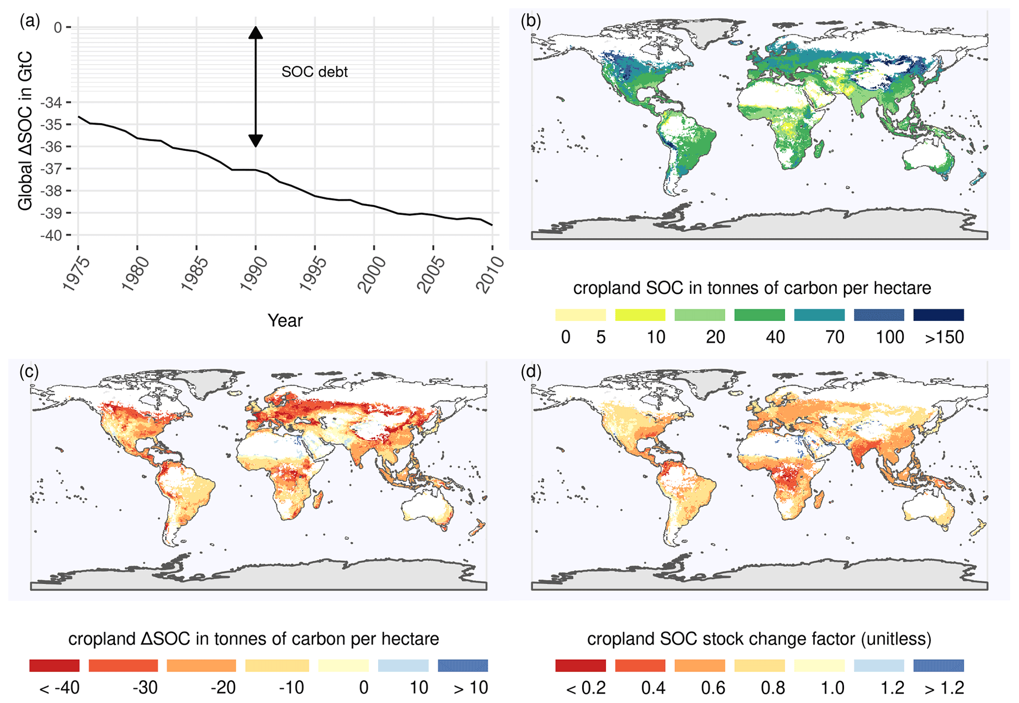
Figure 2Global SOC stocks and SOC stock changes on cropland for the first 30 cm of the soil profile, considering historical management data. Panel (a) shows global ΔSOC between historical land use and potential natural vegetation (PNV). The distribution of total global SOC stocks for the first 30 cm on cropland for the year 2010 is depicted in panel (b). Absolute (c) and relative (d) SOC stocks changes for the year 2010 are compared to a potential natural state to identify different hotspots of SOC losses and gains.
In Fig. 2b, we provide a world map of SOC stock estimates for the first 30 cm on, cropland considering historical management data for the year 2010. Values range between over 100 t ha−1 in northern temperate cropland to less than 5 t ha−1 for arid and semiarid cropland. Our spatially explicit results show hotspots of SOC losses and gains compared to SOC under PNV in the following two complementary ways:
-
Absolute SOC changes ΔSOC (Fig. 2c) indicate areas with high importance for the global SOC loss. They can be driven by large relative changes (e.g., in central Africa) or by a high natural stock from which even small relative deviations could lead to substantial absolute losses (e.g., northeast Asia).
-
Relative SOC changes measured as stock change factors FSCF (Fig. 2d) are a helpful metric to analyze the impact of human cropping activities. They indicate areas with large differences in carbon inflows or SOC decay compared to natural vegetation that may have the potential to be overcome by improved agricultural practices. Large parts of tropical cropland seem to suffer from strongly reduced relative stocks, indicating SOC degradation. Conversely, irrigated cropland at the border of dry, unsuitable areas worldwide shows a strong relative increase in SOC stocks.

Figure 3Global total ΔSOC and ΔSOC change for the first 30 cm of the soil profile. Panel (a) shows global ΔSOC as the difference between SOC under historical land use and SOC under potential natural vegetation (PNV) in the year 2010 summed over all land use types. Computing the difference between the ΔSOC estimate for 2010 and for 1975 (b1) depicts areas of SOC depletion (SOC debt increase; red) and SOC accumulation (SOC debt decline; blue). Panel (b2) shows the land use change (LUC)-induced change in ΔSOC between 1975 and 2010, whereas (b3) depicts the change due to changing agricultural management (MAN).
The spatial distribution of the total ΔSOC summed over all land use types (Fig. 3a), and its change from 1975 to 2010 (Fig. 3b1), reveals areas of SOC debt decline and increase. Regions with large cropland expansion (e.g., Brazil, Southeast Asia, and Canada) continue to lose SOC, whereas regions with cropland reduction (and thus SOC restoration) or with accumulating cropland SOC can be found, e.g., in highly productive areas of Europe and central USA.
3.2 Carbon flows in the cropland system
Carbon is removed from the atmosphere via plant growth and allocated to different plant parts, which we aggregate to three pools (harvested organ and above- and belowground residues). Whereas harvested organs and aboveground residues are taken (partially) from the field to be used for other purposes, belowground residues (729 MtC in 2010) are directly returned to the field. We divide crop biomass usage into feed usage and aggregate all other usage types (e.g., food, bioenergy, and material) into a human demand category. Livestock feed demand for crop organ harvest and aboveground residues of 1136 MtC is roughly equal to the human demand of 1129 MtC. Whereas large parts of feed intake are returned to the soils via manure (C input from manure at 384 MtC), we assume that the carbon demanded from humans (ending up as, e.g., compost, night soil, and sewage) is not returned to soils. Besides manure C and belowground residues, aboveground residues form the largest C input to the soil, with 1350 MtC returned to the fields in the year 2010. However, around 60 % of this organic C decomposes before it is integrated into soils. Due to the different composition of organic C, proportionally more C enters the slow pool from manure than from crop residue. According to our model results, land use change dynamics led to a C transfer from natural vegetation to cropland of 257 MtC in 2010. The cropland system receives 4585 MtC assimilated by crop plants and releases 3554 MtC mostly through respiration. Accounting for SOC transfer and decomposition, the net SOC decrease in global cropland is around 33 MtC for the year 2010.
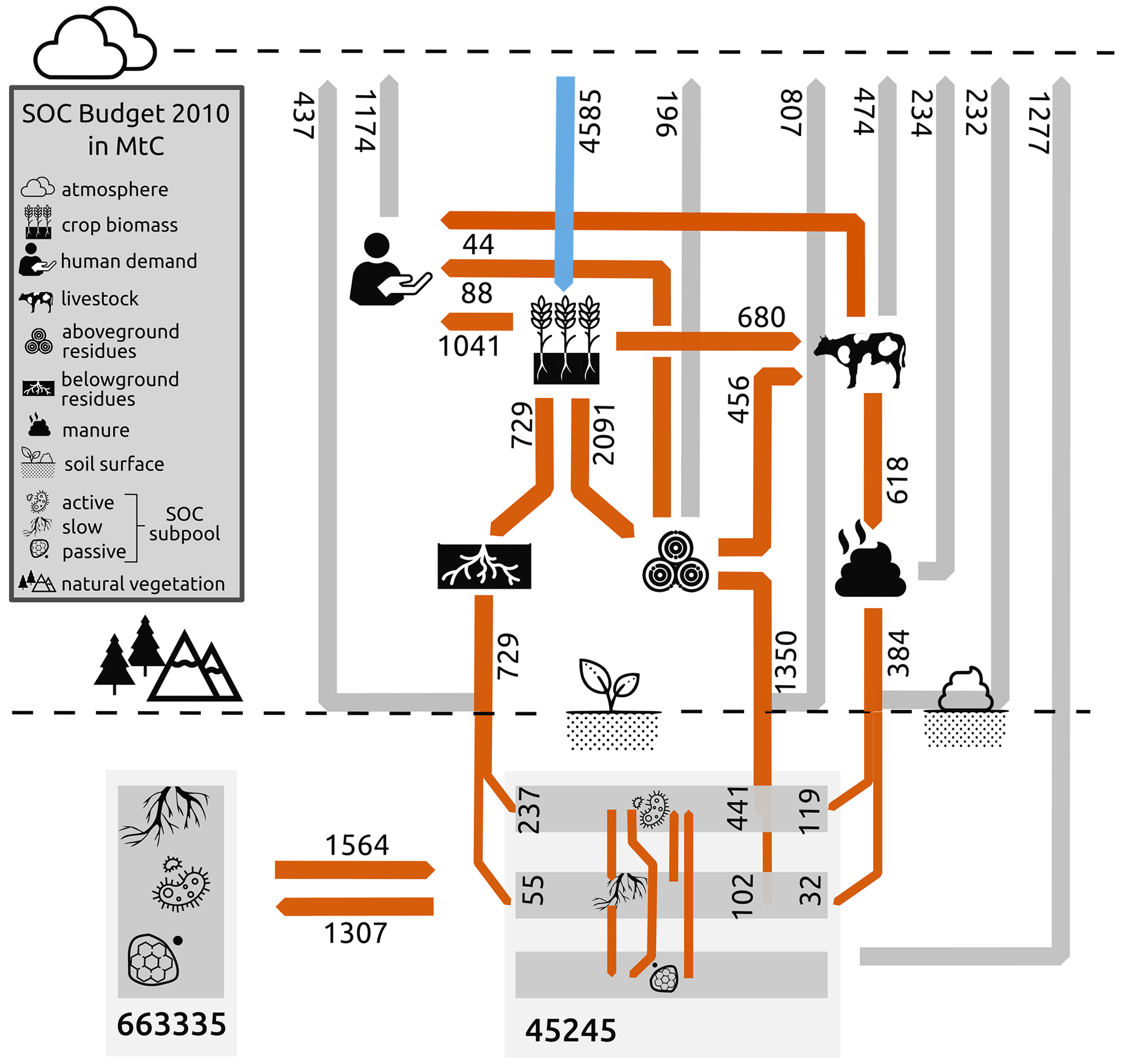
Figure 4Global carbon flows within the cropland system for the year 2010 (in MtC). Carbon is first photosynthesized by crop plants and then used for livestock feed and various other usages subsumed under human demand. After accounting for losses within the cropland system, there are three major C inputs to cropland SOC, i.e., manure and above- and belowground residues. Large parts of C, however, are mineralized on the field before entering the soil. Additionally, C is transferred to and from global cropland soil stock via land use change between cropland and natural vegetation. Finally, SOC is mineralized and flows back to the atmosphere.
3.3 Agricultural management effects on SOC debt
We analyze the relative impact of different management practices by comparing the actual historical management scenario with counterfactual scenarios, where individual management practices (residues in constResidues, manure in constManure, tillage practices in constTillage, and all three in constManagement) are kept static at the 1975 values (Fig. 5a). As shown by the difference between the constResidues scenario and the other counterfactuals, changes in residue return rates dominate the management effects. Without the historical increase in C inputs from residues to agricultural soils, the global ΔSOC would decrease to 41.7 GtC at a rate of 0.20 GtC yr−1 – a 35 % increase compared to 0.14 GtC yr−1 for the historical agricultural management (histManagement estimates). Both the constManure and constTillage scenarios show only small deviations from the historical agricultural management values, with 0.15 GtC yr−1. The effect of no tillage only becomes discernible from 2000 onwards. The large contribution of residues relative to manure also becomes visible when considering the annual C inputs of residues and manure to soils over a period of 35 years (Fig. 5b).
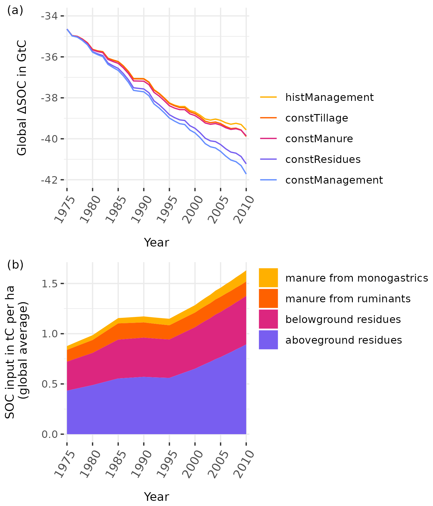
Figure 5(a) Global ΔSOC (in GtC) for different management scenarios. The stylized scenarios deviate from historical agricultural management patterns (histManagement) by holding the effects of carbon inflows from residues (constResidues) or manure (constManure) constant at the 1975 level or neglecting adoption of no-tillage practices over time (constTillage). The scenario of constManagement combines all three modifications. Note that ΔSOC is defined as the difference in SOC under land use compared to a hypothetical natural vegetation state. Panel (b) shows the carbon inflows from crop residue and manure.
Using the constManagement results that only include land use change (LUC)-related changes in the SOC debt between 1975 and 2010, we are able to subtract the LUC effect from the overall SOC debt change within the histManagement results. The remaining effect can be attributed to the changing agricultural management (MAN), as other drivers such as climatic effects have been already canceled out by taking the difference to a PNV reference state when calculating ΔSOC. The increasing SOC debt on global cropland are primarily caused by LUC (red areas in Fig. 3b2). Deteriorating management also contributed to increasing SOC debt in parts of sub-Saharan Africa and central Asia. In contrast, agricultural management has led to an decrease in SOC debt in the USA, Europe, and in parts of China and India (blue areas in Fig. 3b3), which is not visible in the total ΔSOC change, as LUC was happening at the same time.
Our sensitivity analysis shows that the management impact is robust to the initialization of SOC stocks (see Fig. A2 and Sect. 2.4), with around 2.15 GtC difference in SOC debt between the histManagement and the constManagement scenarios. However, the SOC debt and SOC debt change vary with the different initialization choices. Whereas the default assumption (Initial-spinup1510) shows a ΔSOC of 39.6 GtC for the year 2010, the Initial-natveg scenario with high legacy fluxes to come only has a ΔSOC of 33.3 GtC, and the Initial-eq scenarios with only a few legacy fluxes already left a ΔSOC of 50.7 GtC.
3.4 Model evaluation
To evaluate our model results against reference data, we (1) compare our stock change factors (see Sect. 2.2) to IPCC default assumptions (chap. 5 in IPCC, 2006, 2019), (2) compare our global (and climate-zone-specific) total SOC stocks to other literature estimates, and (3) compare our results to point measurements. To evaluate the representation of our natural SOC stocks, we (4) correlated LPJmL4 SOC stocks for PNV with our natural state SOC results on grid level and (5) did a similar correlation analysis for our modeled actual SOC stocks in comparison to the results of SoilGrids 2.0 (Poggio et al., 2021), which accounts for actual land use too.
3.4.1 Stock change factors compared to IPCC assumptions
To evaluate our modeled SOC stocks and stock changes under agricultural management, we compare our results to the default IPCC stock change factors FSCF of 2006 (IPCC, 2006, chap. 5) and their refinements in 2019 (IPCC, 2019, chap. 5). Both estimates are based on measurement data for cropland (see Fig. 6). To allow for comparison, we aggregate our stock change factors weighted by grid-level cropland area to derive median factors for the four IPCC climate zones (Fig. A1 in Appendix A). Note that IPCC tier 1 factors are derived under the assumption that there is a linear change between steady states over 20 years, whereas our aggregated factors just reflect the relative change compared to a given potential natural vegetation reference stock without specifically tracking the age of the cropland.
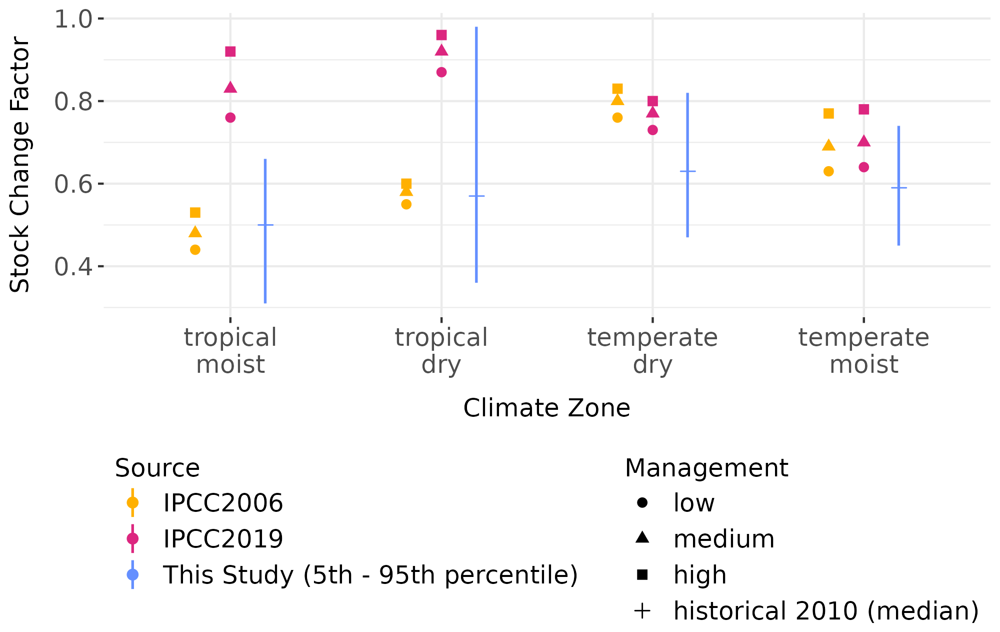
Figure 6FSCF in comparison to IPCC tier 1 default factors from the guidelines in 2006 (IPCC, 2006, chap. 5) and the update in 2019 (IPCC, 2019, chap. 5). IPCC factors vary a bit with different types of management (low, medium, and high). The results of the study span over a wide range – indicated by the span between the 5th and 95th percentile – but do not overlap with the IPCC 2019 factors for tropical moist regions. The median for most regions is considerably lower than the IPCC factors.
Stock change factors for the temperate climate zones of this study are lower than the default values of the IPCC. For the tropical regions, the IPCC factors increased notably from the guidelines in 2006 (IPCC, 2006, chap. 5) to the update in 2019 (IPCC, 2019, chap. 5) due to the inclusion of more data points. Our results span over a broad range due to the different ages of the cropland but also due to different agricultural management practices within climate regions.
3.4.2 Global SOC stocks comparison
We compare our global SOC stocks with a wide range of global SOC stock estimates for the first 30 cm of the soil profile, using data from WISE (Batjes, 2016), SoilGrids (Hengl et al., 2017), GSOC (FAO, 2019), LPJmL4 (Schaphoff et al., 2018a), SoilGrids 2.0 (Poggio et al., 2021), and SOCDebtPaper (Sanderman et al., 2017) in Fig. 7.
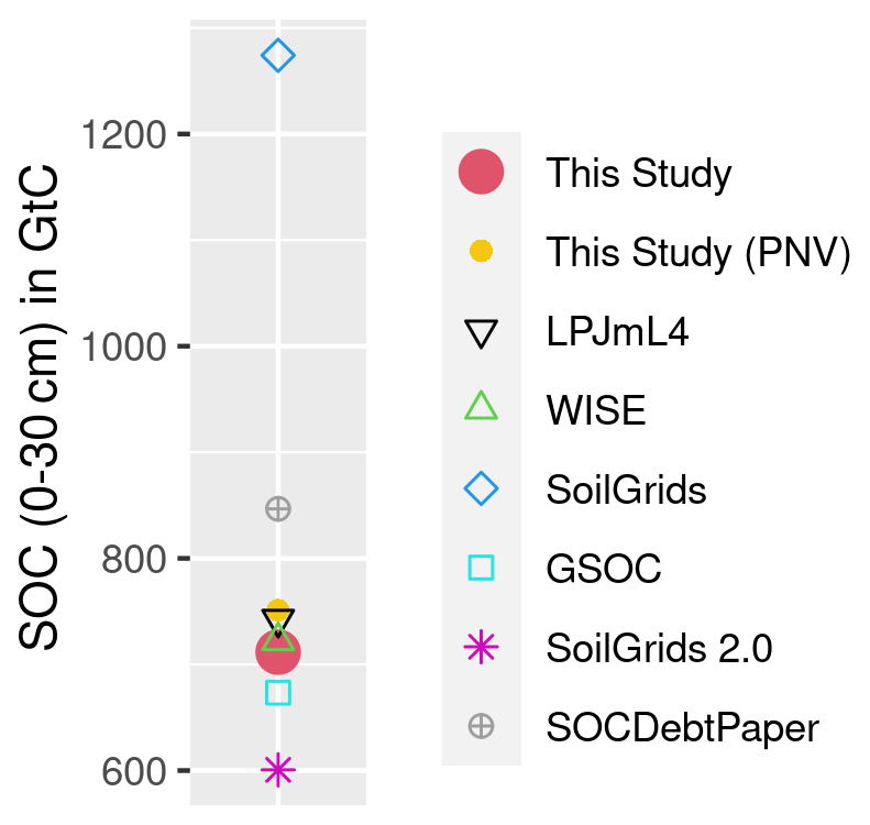
Figure 7Modeled and observation-based estimates for global SOC stock (in GtC) for the first 30 cm of soil aggregated over all land areas. The comparison against observation-based data (SoilGrids, SoilGrids 2.0, GSOC, and WISE) is supplemented by modeled data from LPJmL4 (Schaphoff et al., 2018a) and estimates from Sanderman et al. (2017). We show values of this study for the year 2010, accounting for the historical land use dynamics and for a hypothetical PNV.
The global estimates of the total SOC stock of the upper 30 cm from this study are in the middle of the wide range of other modeled or observation-based estimates. Regional results (Fig. A3) show that our estimates are well within the range of other estimates for most regions but at the lower end for tropical moist and tropical wet areas. SoilGrids (Hengl et al., 2017) especially stands out with its high estimate, since this model includes the litter horizon on top of the soil that might dominate especially polar and boreal soils. SoilGrids 2.0 (Poggio et al., 2021), however, excludes litter C and thus marks the lower end particularly for northern regions. For the same reason, it is also more comparable to our results, which also do not account for litter C.
3.4.3 Point-based evaluation
In Fig. A4, we correlate our SOC results for natural vegetation and cropland in 2010 with the literature values of point measurements (for the database, see the Appendix in Sanderman et al., 2017). The goodness of the fit is very low, with an R2 of 0.13. Individually, the correlations are even lower, with a R2 of 0.09 for cropland and 0.08 for areas of natural vegetation. This points to the fact that differences between land use type SOC stocks could be better matched than the spatial pattern of the rather small point measurement database. Due to the low number of small-scale measurements, statistical properties of the point data variability are not derived and, thus, could not be used to improve the point-to-grid-cell comparison (see Rammig et al., 2018).
3.4.4 Natural SOC stock comparison with LPJmL4
Estimates of SOC stocks under natural vegetation influence our modeled results for cropland, which has been converted from natural vegetation at some point in time. As the tier 2 modeling approach (IPCC, 2019, chap. 5) is not specifically parameterized for natural vegetation, it is important to evaluate its suitability for producing reasonable results in that domain that are at least comparable to other modeling approaches. We therefore also compare our modeled results for SOC under natural vegetation (derived using the litterfall of LPJmL4) against estimates of SOC by LPJmL4 for a PNV simulation (see Fig. A5). Both models are driven by the same climate conditions and the same natural litterfall and just differ in the representation of SOC and litter dynamics. With our focus on cropland SOC dynamics, we compare only cells with more than 1000 ha of cropland (capturing 99.9 % of global cropland area). Spatial correlations of PNV SOC stock values are high (global R2=0.81), especially for dry climate zones (Fig. A5). For temperate and tropical moist areas, estimates of this study tend to be a bit lower compared to the LPJmL4 results.
3.4.5 Actual SOC stock comparison with SoilGrids 2.0
SoilGrids 2.0 (Poggio et al., 2021) is a digital soil mapping approach that uses over 240 000 soil profile observations to produce high-resolution soil maps, including SOC stocks and estimates of their uncertainties. To evaluate the performance of our model at the global scale, we correlate SoilGrids 2.0 SOC stock values, which were aggregated to 0.5∘ resolution, to our estimates for the year 2010 in Fig. 8. To focus our comparison on cropland areas, we mask out grid cells with fewer than 1000 ha of cropland. The spatial correlation is moderate for tropical climate zones, whereas it is low for temperate moist areas. In tropical dry and temperate dry areas, we also simulate very low SOC values (below 10 tC ha−1), which is not found in SoilGrids 2.0, whereas our modeled SOC stocks can be substantially higher than those reported by SoilGrids 2.0 in temperate moist areas. Additionally, we use the uncertainty estimates from SoilGrids 2.0 in Fig. 9 to identify areas where our modeled SOC stocks are below the 5th or above the 95th percentile of the SoilGrids 2.0 data. For the vast majority of grid cells, our model results are between the 5th and 95th percentile of SoilGrids 2.0 estimates. We underestimate SOC stocks, especially in dry areas (e.g., close to the Sahara). Overestimated stocks are often situated in mountainous regions.

Figure 8Correlation between modeled SOC stocks of this study and projected values from SoilGrids 2.0.
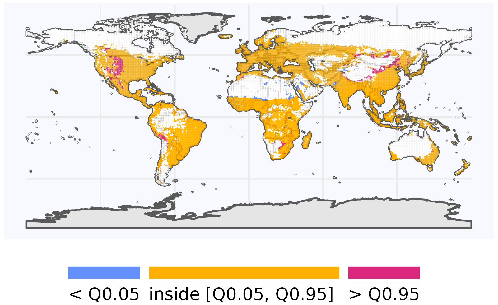
Figure 9Global map on SOC results compared to uncertainty estimates from SoilGrids 2.0 (Q0.05 – 5th percentile; Q0.95 – 95th percentile).
We have (1) developed a reduced-complexity model and (2) compiled a spatially explicit time series data set of agricultural management data in order to (3) analyze the role of agricultural management in historical cropland SOC dynamics. Our study shows that information on agricultural management alters estimates of the SOC debt and slows down the loss of SOC compared to the often-used constant management assumptions.
It is important to evaluate the validity of our results, as modeling management effects on SOC dynamics at the global scale come with large uncertainties. The model includes a large number of parameters, and for most of these, the uncertainty distributions have not been quantified so far. Moreover, we think that, beyond parameter uncertainty, the structural uncertainty of the model design is high. The management data itself are prone to uncertainties as well, as most of the data are only indirectly calculated from reported data.
In the following, we give a qualitative assessment of the uncertainties and limitations of this study and discuss our three study objectives and results against the existing literature.
4.1 Comprehensive historical agricultural management data set
Our spatially explicit time series data set of agricultural management is based on country-specific FAO production and cropland statistics (FAO, 2021) and 0.5∘ land use data from LUH2 (Hurtt et al., 2020). Starting from these two sources, we derive a harmonized and consistent data set for the major C flows within the cropping system (Fig. 4) using a mass balance approach from the IPCC guidelines vol. 4 (IPCC, 2006, 2019) and other auxiliary data sets (e.g., Porwollik et al., 2019).
For some of the aspects covered in our data set, for example, livestock distribution (Robinson et al., 2014) or manure production and application (Zhang et al., 2017), well-compiled data sets in high resolution exist that capture real-world conditions much better than our estimates. However, they often come with the caveats of either being static in time, demanding large sets of auxiliary data, or being inconsistent with each other.
For most of the parameters used in our management estimates, no uncertainty estimates exist. This is why, in our view, a large part of the uncertainty with respect to the impact of SOC management – next to the parametric and structural uncertainty of the soil model – is included in the management data itself. This is especially the case for the residue and manure production and application numbers, as these are only indirectly derived from crop and livestock production, feed data, and area data (FAO, 2021; Weindl et al., 2017). The uncertainty of recycling shares adds, on top of the uncertain total, numbers of manure and residue biomass. Previous modeling studies of SOC carbon on cropland often only used stylized scenarios of management practices (Pugh et al., 2015; Lutz et al., 2019) rather than trying to estimate real management.
While our data set includes crop residues and manure, which are likely the largest carbon inputs to soils, it does not account for a list of minor carbon inputs from cover crops, agroforestry, green manure, weed biomass and the application of human excreta, sewage sludge, processing wastes, forestry residues, or biochar. Including these sources would correct our estimates upwards and bring our estimates closer to the IPCC stock change factors (see Sect. 3.4.1). Unfortunately, data on the quantity of these inputs are very scarce and do not exist with global coverage.
SOC inputs from aboveground residues had the strongest management effect on SOC debt dynamics on cropland (see Fig. 5). As pointed out by Keel et al. (2017) and Smith et al. (2020), carbon input calculations are highly sensitive to the choice of allometric functions determining below- and aboveground residue estimates from harvested quantities (see Table A1 in Appendix A, for coefficients used in this study). Keel et al. (2017) question whether belowground residues might increase with a fixed root-to-shoot ratio rather than being independent of productivity gains. Moreover, the study pointed out that plant breeding shifts allometries, which might not be reflected in outdated data sources. While our study considers a dynamic harvest index with rising yields for several crops, we may still overestimate residue biomass, in particular for belowground biomass.
4.2 Reduced complexity SOC model
Our reduced-complexity SOC model is based on a tier 2 modeling approach. This reduces the computational and data demand of the model in comparison to DGVMs, while still allowing for the explicit representation of agricultural management practices. Along with the effects of various C inputs, the impacts of water supply from rainfall and irrigation and tillage systems can also be accounted for in the computation of SOC decay rates. As such, the model can reflect the spatial and temporal heterogeneity in both management and biophysical conditions.
The substantial impact of changing management practices through time is indicated by the development of our estimated stock change factors (see Fig. 6) and by the time trend of the SOC debt (see Fig. 2a). Residue management has changed over the last few decades, especially with the phasing out of residue burning practices in several regions and increased general productivity, showing a clear impact on SOC dynamics and underlining the importance of accounting for these effects in soil carbon modeling.
The tier 2 approach (IPCC, 2019, chap. 5) used here is explicitly designed for agricultural soils, whereas we also apply it to soils under PNV. This is necessary in order to represent SOC losses under land use change in a dynamic way, as this is an important driver of SOC dynamics. The comparison of simulated PNV data with LPJmL4 shows the model's capability in reproducing PNV SOC stocks (Fig. A5). Concurrently, the point data comparison (see Fig. A4) shows low correlation for PNV and also for cropland sites. This might point to the fact that SOC stocks can vary considerably at field and local scales and thus a very high number of point data is needed to derive statistical properties that could improve the point-to-grid-cell comparison (see Rammig et al., 2018).
Using litterfall estimates from LPJmL4, we have been able to estimate the total SOC stocks of the world which are dominated by SOC under natural vegetation. However, as the world's SOC stock is highly uncertain, which is seen in the wide range of global SOC stock estimates for the first 30 cm of the soil profile (Batjes, 2016; Hengl et al., 2017; FAO, 2019; Schaphoff et al., 2018a; Poggio et al., 2021; Sanderman et al., 2017) in Fig. 7, the only conclusion we can draw from this is that our result is within a plausible range.
Additionally, we find our 0.2 GtC yr−1 SOC stock change within the period between 1975 and 2010 for the first 30 cm of the soil profile at the upper end of estimates when comparing it to estimates by Ito et al. (2020) of 0.18 ± 0.41 GtC yr−1 within the period between 1850 and 2014 for whole soil profile. This might be unsurprising, as the CO2 effect is most likely stronger and the land use change effects weaker within our later and shorter modeling period compared to a mean value of the period between 1850 and 2014. The large uncertainty within the estimates of SOC stock and its changes (Ito et al., 2020) again points to the large structural uncertainty within SOC modeling.
To avoid a strong impact of natural land representation and its uncertainties on our results, we focus on SOC changes on cropland. Pristine natural vegetated areas (like permafrost and rain forests) without human land management drop out in our calculation of SOC debt and stock change factors. Natural SOC estimates only influence results when natural land is converted to cropland. Moreover, the temporal dynamic of the SOC debt and stock change factors is not (or is only to a small degree) altered by climatic or atmospheric effects on SOC stocks, as they are canceled out by taking the difference (for the SOC debt) and ratio (for the stock change factors) of cropland SOC and SOC under hypothetical PNV conditions.
The initialization of SOC stocks, however, is important for the size of the SOC debt and its change over time, since the presence and size of legacy fluxes affect these values strongly (see Fig. A2). According to our sensitivity analysis, the SOC debt varies between 33.3 and 50.7 GtC, depending on the initialization choice, with our best guess at 39.6 GtC. Concurrently, our results indicate that the impact of the dynamic agricultural management is robust to the initialization of SOC stocks.
Comparing the geographic SOC patterns to SoilGrids 2.0 (Poggio et al., 2021, see Fig. 9), we find that our model estimates values of SOC stocks that are greater than the estimated confidence intervals in SoilGrids 2.0 for some mountainous regions across the globe. This could indicate that we are not capable of capturing specific processes that would reduce the vegetation's productivity (such as erosion on steep slopes or shallow soils; Borrelli et al., 2017). A large swathe of eastern North America was heavily affected by a dust bowl event, with wind erosion removing large parts of the topsoil, a process not considered in our model. Similarly, we likely overestimate SOC stocks for the loess soils in northern China and the Altiplano in Latin America; in both cases, erosion is a likely reason. In contrast, we estimate lower SOC stocks at the edges of the Sahara, where uncertain local water availability and artificial irrigation may dominate spatial SOC patterns.
In our model, erosion might, however, only affect the spatial pattern but not the aggregate SOC pool. As pointed out by Doetterl et al. (2016), the final fate of leached or eroded carbon is uncertain and might even offset LUC emissions (Wang et al., 2017). Concurrently, other studies have claimed erosion moves SOC into aquatic reservoirs (Zhang et al., 2020), thus changing the total global terrestrial SOC stock. Whereas SOC displacement might play an important role for soil quality analysis, in this budget approach, focused especially on the SOC debt, displaced but not emitted SOC can be treated as SOC that remains on the cropland. Erosion and degradation impacts on yields and therefore on soil C inputs are captured by our method, as we base them on FAO statistics of actual production. Yet the distribution of production below the country level – which we allocate proportional to LPJmL production potentials that do not reflect erosion feedback to yields – will overestimate yields and therefore biomass inputs to eroded soils.
In comparison with default stock change factors of the IPCC guidelines, our model estimates a stronger decline in SOC stocks (Fig. 6) for almost all regions. Tropical soils might suffer from low C input rates due to large yield gaps (Global Yield Gap Atlas (GYGA); https://www.yieldgap.org, last access: 3 January 2022) and high shares of residue removal and burning in lower-income countries (Smil, 1999a; Williams et al., 1997; Jain et al., 2014). Yet, even when comparing our estimates to the low-input stock change factors of the IPCC, our SOC loss is roughly twice as large as the revised 2019 IPCC default values (IPCC, 2019, chap. 5), while it shows good agreement with the older default values from IPCC (2006, chap. 5). However, the revised estimates of the IPCC included many more and more recent data points, calling for a closer look at causes of the large deviations between our results and the refined tier 1 factors. On the one hand, our approach does not account for unharvested carbon inputs from weeds or biomass cover on short-term fallows. Shifting agriculture with fallow periods might be prominent in tropical regions. While long-term fallow land (>4 years) is excluded from FAOSTAT as cropland, short-term fallow is not. Thus, our carbon inputs for these areas might be underestimated, leading to too low stock change factors. On the other hand, older studies by Don et al. (2011) estimated SOC losses for tropical soils of around 25 % on average, corresponding to a stock change factor of 0.75, but also reported a wide range of measured SOC changes from −80 % to +58 %. Fujisaki et al. (2015), however, found much lower loss rates of around 9 %, attributing the difference to the different time period lengths since the conversion to cropland. As our results do not specifically account for cropland age, and most of the cropland is older than 20 years (as assumed for the default IPCC tier 1 stock change factors), our stock change factors have to be lower by definition, following the steady-state assumption that cropland will continue to approach a new equilibrium. For the same reason, our estimates for temperate regions might be lower than those default values of both IPCC (2006, chap. 5) and IPCC (2019, chap. 5). With the production-increasing impact of irrigation and fertilization on carbon-poor dryland soils, SOC under cropland can also be higher than under PNV with stock change factors above 1 (see Fig. 2d), but these areas are much smaller than where the stock change factors are well below unity.
Generally, limiting the analysis to the first 30 cm of the soil profile follows the IPCC guidelines (IPCC, 2006, 2019) and assumes that most of the SOC dynamics happen in the topsoil. In this regard, several aspects are strongly simplified within our approach. First, the distribution of carbon inputs into different soil layers are neglected, and all carbon inputs are allocated to the topsoil. This particularly overestimates SOC stocks in the first 30 cm of soil below deeper rooting vegetation, which is certainly the case for most of the woody natural vegetated areas. Second, changes to the subsoil are neglected, which is most important for tillage effects. Other management practices might be more equally affecting topsoil and subsoil, as they do not directly the relocates carbon vertically. As Powlson et al. (2014) have shown, the subsoil can be make a large difference in the evaluation of total SOC losses or gains for no-tillage systems. No-tillage effects may seem larger than they actually are if only topsoil is considered. SOC transfers to deeper soil layers under tillage might enhance subsoil SOC compared to no-till practices. However, the effect of no till on the subsoil and its overall importance as a SCS measure is still debated (Ogle et al., 2019). Finally, organic soils (like peatlands and wetlands) and drained cropland areas are not explicitly considered, and emissions from these cropland areas are thus likely substantially underestimated.
4.3 SOC debt and SOC drivers
The analysis of SOC stock gains and losses is complex and has several dimensions as climatic and anthropogenic effects overlap. There is broad consensus that land conversion to cropland has caused substantial C emissions over the historical period (e.g., Friedlingstein et al., 2020). There is uncertainty with respect to the overall size of these emissions from different methods and reference points and with respect to the contribution of cropland and agricultural management to these emissions. In order to mitigate greenhouse gas emissions, it is essential to stop the decline of SOC stocks or even transform cropland management to sequester atmospheric C in cropland soils (Minasny et al., 2017). Defining the SOC debt of 1975 as the baseline, and measuring land use emissions on cropland as the difference between a potential natural state and the state under human interventions (see Pugh et al., 2015), we find that global cropland has acted as an emissions source since 1975. Comparing our SOC loss rate (the change in SOC debt) of 0.14 GtC yr−1 to estimates of land-use-change-induced emissions of 2.0 ± 1.0 GtC yr−1 (sum of bookkeeping land use and land cover change (LULCC) emissions and loss of additional sink capacity for the years 2009–2018 in Gasser et al., 2020), we find SOC emissions of the first 30 cm of the soil profile to be a minor contributor to overall land-use-change-induced emissions. Annual C loss rates of 0.2 per 1000 C still have the opposite trend to the promoted 4 per 1000 C sequestration rate target (Minasny et al., 2017). Dedicated efforts to increase cropland SOC are thus necessary, as management improvements at historical rates are not enough to counteract ongoing SOC degradation on cropland. Yet our study also shows the substantial impact of changing management on the development of SOC debt (Figs. 3 and 5).
According to Sanderman et al. (2017), the SOC debt since the beginning of human cropping activities has been at around 37 GtC for the first 30 cm of the soil, with half of it attributed to SOC depletion on grasslands. Our estimate of 39.6 GtC in 2010 for cropland debt is thus twice as high as their estimate. However, there are large uncertainties in modeling SOC at the global scale, and Sanderman et al. (2017) pointed out that their results might be conservatively low compared to experimental results.
Furthermore, Sanderman et al. (2017) modeled historical trends based on agricultural land expansion without considering SOC variations due to time-variant agricultural management. Pugh et al. (2015) considered management effects like tillage and the incorporation of residues in stylized and static scenarios only so that they could not account for the historical management effects on SOC dynamics. Their study, moreover, concludes that yield gains (by 18 % in their simulations) do not lead to a substantial decline in SOC debt (less than 1 % SOC increase). Historical yield increases, however, are estimated to be well above 50 % (Pellegrini and Fernández, 2018; Ray et al., 2012; Rudel et al., 2009) and often lead to an increase in below- and aboveground residue biomass inputs to the soil. While we find substantially larger SOC increases in response to productivity gains than the 1 % reported by Pugh et al. (2015), this is not sufficient to compensate SOC losses from the global cropland expansion of around 11 % between 1974 and 2010.
The effects of agricultural productivity on cropland SOC dynamics, including historical yield trends and associated increases in residue inputs, can be directly accounted for in our modeling approach. In contrast, process-based studies (Pugh et al., 2015; Herzfeld et al., 2021) often lack data on relevant management aspects that drive production increases. Herzfeld et al. (2021) also consider historical management trends for fertilizer and manure inputs and on residue removal rates and tillage systems but cannot reproduce the substantial increase in agricultural productivity over the last few decades. Still, they find that, compared to no-tillage systems, residue management has much larger potential to affect the strength of their projected future global cropland SOC decline. This is consistent with our finding that increasing SOC inputs from aboveground residues had the strongest effect on the slowing down of the SOC debt increase (Fig. 5). In line with this, Dangal et al. (2022) find that no tillage has only minor impacts on SOC dynamics across parts of the USA.
Elliott et al. (2018) show that yield trends in the USA can be reproduced by models but require information on inputs that are not available at the global scale, such as annual data on sowing dates, planting densities, and genetic traits such as kernel number and radiation use efficiency. As such, it will remain challenging for process-based DGVMs to capture the trend of agricultural productivity on cropland SOC dynamics.
Our study emphasizes again that the expansion of cropland is still a major source of CO2 emissions – not only through the removal of vegetation but also by a slow depletion of C stocks in soils. Our estimates indicate a SOC debt of 39.6 GtC in 2010, and every additional deforested hectare adds to this debt. Avoided deforestation and other environmental regulation leads to an intensification on existing cropland (Humpenöder et al., 2018), and our results show that such an intensification could lead to increased cropland SOC if residues are returned to the soil, amplifying the C sequestration potential of avoided deforestation.
There is also ample potential for further improved SOC management. As shown in Fig. 4, the annual SOC respiration (1.3 GtC yr−1) is slightly above one-quarter of the total annual net C uptake by crops (4.6 GtC yr−1). C compounds have to be respired by soil organisms to maintain basic soil functions and regulate the nutrient cycle, which often leaves limited options to decrease C losses via SOC respiration (Janzen, 2006). However, similar C losses occur at the end of the food supply chain (1.2 GtC yr−1), at the soil surface (1.5 GtC yr−1), and are smaller but still considerable during residue burning (0.2 GtC yr−1) and within animal waste management systems (0.2 GtC yr−1). Improved management could include, first, a circular flow from the food supply chain back to soils. Waste composting or excreta recycling could represent a major additional C input to cropland soils (Brenzinger et al., 2018). Second, soil carbon sequestration techniques (Smith, 2016), deep plowing (Alcántara et al., 2016), or the transformation of C inputs to more recalcitrant biochar (Woolf et al., 2010) may transfer larger parts of the biomass at the litter soil barrier into permanent soil pools. Third, reducing the share of residue burning and improved manure recycling could further increase C inputs. Finally, other carbon accumulating practices, such as the cultivation of cover crops (Poeplau and Don, 2015; Porwollik et al., 2022) and agroforestry (Lorenz and Lal, 2014), could increase total C sequestration on cropland.
We have compiled a spatially explicit and time-variant data set on agricultural management aspects relevant for cropland SOC dynamics. We have also developed a reduced-complexity SOC model that is able to be applied in optimization-based IAM frameworks, for which detailed process-based models are computationally too expensive. Making use of these data and this model, we are able to estimate spatially explicit SOC stocks, SOC debts, and stock change factors considering agricultural management. It is – to our knowledge – the first study that analyzes the role of time-variant and spatially explicit historical agricultural management for global SOC dynamics.
Our results demonstrate that historical changes in agricultural management have shaped the SOC debt on cropland. It is thus necessary to explicitly consider agricultural management in a dynamic manner in global carbon assessments and models, especially when exploring climate mitigation pathways with so-called land-based solutions (e.g., Popp et al., 2016). That also implies that we not only need better monitoring of agricultural practices to create these data but also better accessibility of existing data. Our open-source model (Karstens and Dietrich, 2022), published data set (Karstens, 2022), and the flexible data processing with the MADRaT package (Dietrich et al., 2022) constitute a starting point for building comprehensive data sets on agricultural management aspects.
With the reduced-complexity SOC model, we are able to account for agricultural management effects on cropland SOC dynamics within optimization-based IAM frameworks. Reduced input data requirements such as accounting for changes in productivity rather than reproducing the processes that lead to such changes in productivity (Elliott et al., 2018) will help us to explore the role of agricultural management in sustainable development pathway analyses (Sörgel et al., 2021). However, we clearly see that increases in agricultural productivity are not sufficient to create positive net SOC sequestration in cropland soils. More management options that explicitly target the sequestration of C in cropland soils need to be considered. Our open-source model can be expanded to account for additional management options for carbon farming, such as cover crops, agroforestry, or biochar applications.
A1 Methods

Figure A1Climate zone map adapted from IPCC. The climate zone classification is based on the classification scheme of the IPCC guidelines (IPCC, 2006) and has been reimplemented by Carre et al. (2010), which is the source of these data. Note that the reduced set, used for the comparison of stock change factors, is included in the color code, with temperate moist in light blue, temperate dry in dark violet, tropical moist in red, and tropical dry in orange.
Table A1Parameterization of harvested organs and their corresponding residues parts and allometric coefficients. This table is mainly based on Bodirsky et al. (2012), together with simple carbon to dry matter assumptions. Allometric coefficients are used, as described in IPCC (2006), with HIprod being slope(T), HIarea intercept(T), and RS RBG-BIO.

– nitrogen-to-dry-matter ratio; – wet-matter-to-dry-matter ratio; – carbon-to-dry-matter ratio; HIarea – harvest index per area; HIprod – harvest index per production; RS – root : shoot ratio.
A2 Results
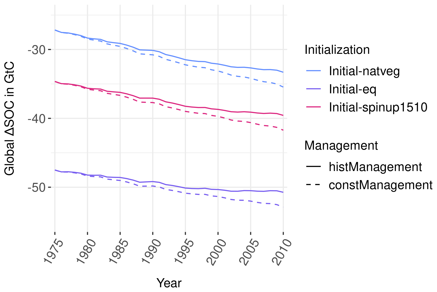
Figure A2Global ΔSOC for different SOC initialization choices in the start year of 1901. Starting in 1901 with steady-state SOC under vegetation for all land use types without any human cropping activities (Initial-natveg) leads to a smaller ΔSOC in 1975 and a steeper increase until 2010, as compared to initializing with steady-state SOC stocks under historic land use (Initial-spinup1510). On the other hand, assuming all SOC to be in a land-use-specific steady state already in 1901 (Initial-eq) leads to the opposite effect of an already higher ΔSOC in 1975 and a less steeper increase until 2010. However, the difference between the dynamic historical management assumption (histManagement) compared to constant management assumption from 1975 onward (constManagement) is of a similar size for all initialization choices.
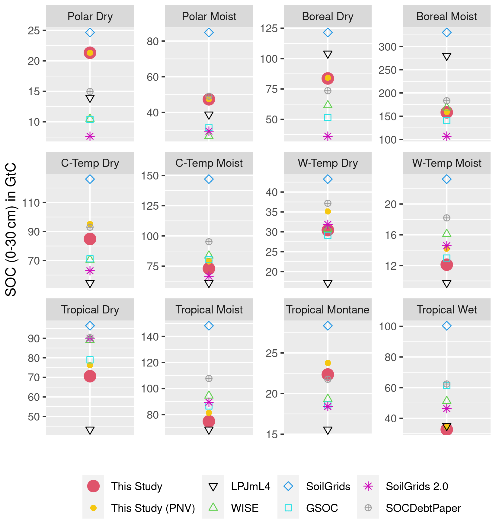
Figure A3Modeled and data-based estimation for climate-zone-specific SOC stock (in GtC) for the first 30 cm of soil aggregated over all land areas. SoilGrids, GSOC, and WISE do not consider changes over time and rely on soil profile data gathered over a long period of time, which makes it hard to pinpoint a specific year for these SOC estimations. In this context, they will be compared to modeled data (LPJmL4; this study) for the year 2010. PNV denotes the potential natural vegetation state, without considering human cropping activities, calculated as reference stock within our model. We use the climate zone specification of the IPCC (IPCC, 2006).
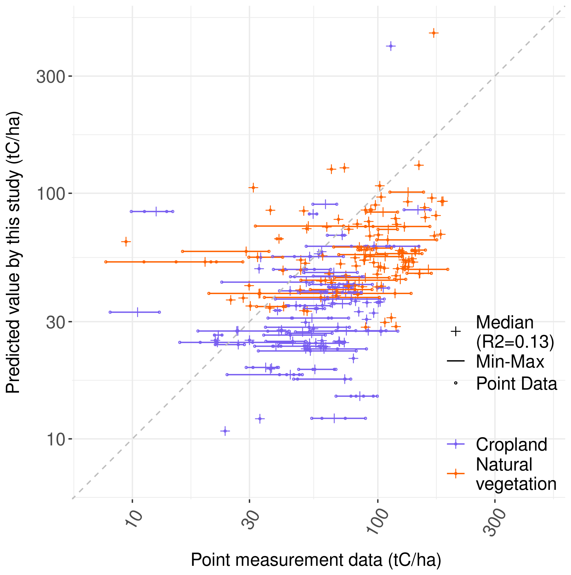
Figure A4Correlation between modeled and measured SOC stocks. Given the wide span between minimum and maximum measured SOC stocks within in a given cell, we correlated the median values with our modeled results. Both cropland (R2=0.09) and areas with natural vegetation (R2=0.08) tend to be lower in our results than in the point measurements.

Figure A5Correlation between modeled SOC stocks of LPJmL4 and this study for a hypothetical potential natural state (PNV) for the year 2010. The gray lines indicate the 1 : 1 line.
We compiled our calculations as open-source R packages that are available at https://doi.org/10.5281/zenodo.7234094 (Bodirsky et al., 2022a), for the management-related functions, https://doi.org/10.5281/zenodo.6330155 (Karstens and Dietrich, 2022), for soil dynamic related functions, and https://doi.org/10.5281/zenodo.7234083 (Bodirsky et al., 2022b), for validation data. All libraries are based on the MADRaT package available at https://doi.org/10.5281/zenodo.7234107 (Dietrich et al., 2022), a framework which aims to improve the reproducibility and transparency in data processing. Model results, including C input data, are accessible at https://doi.org/10.5281/zenodo.4320663 (Karstens, 2022). The software code for the paper and result preparation can be found under https://doi.org/10.5281/zenodo.7234651.
KK, BLB, AP, and HLC designed the study and the model idea. KK wrote the code built on work of BLB and IW. JPD revised and improved the model code. CM, JH, and SR provided the LPJmL simulation data. MK, MD, PS, JH, and CM provided feedback on the soil modeling part. KK wrote the paper, with important contributions from BLB and CM. MK, JS, SR, and IW provided extensive feedback to the outline of the study. All authors discussed the results and commented on the paper.
The contact author has declared that none of the authors has any competing interests.
Publisher’s note: Copernicus Publications remains neutral with regard to jurisdictional claims in published maps and institutional affiliations.
Thanks to Vera Porwollik, for contributing the time-resolved tillage data set based on her previous work. Additional thanks go to the article contributors, for providing an R Markdown template. The authors are grateful for the data provided by FAOSTAT and LUH2v2.
The work of Kristine Karstens has been funded by the DFG Priority Program “Climate Engineering: Risks, Challenges, Opportunities?” (SPP 1689), specifically the CEMICS2 project (grant no. ED78/3-2), and by the CDRSynTra project (grant no. 01LS2101G) funded by the German Federal Ministry of Education and Research (BMBF). The research leading to these results has received funding for Benjamin Leon Bodirsky from the European Union's Horizon 2020 Research And Innovation Programme (grant nos. 776479 (COACCH) and 821010 (CASCADES)). Benjamin Leon Bodirsky acknowledges support by the project ABCDR (grant no. 01LS2105A) funded by the BMBF. The work of Susanne Rolinski, Jens Heinke, and Isabelle Weindl has also been supported by CLIMASTEPPE (grant no. 01DJ8012), EXIMO (grant no. 01LP1903D), and FOCUS (grant no. 031B0787B), all funded by the BMBF. The input of Pete Smith, Matthias Kuhnert, and Marta Dondini contributes to the Soils-R-GGREAT project (grant no. NE/P019455/1) and CIRCASA (EU H2020; grant no. 774378).
This paper was edited by Sönke Zaehle and reviewed by Jonathan Sanderman and two anonymous referees.
Alcántara, V., Don, A., Well, R., and Nieder, R.: Deep Ploughing Increases Agricultural Soil Organic Matter Stocks, Glob. Change Biol., 22, 2939–2956, https://doi.org/10.1111/gcb.13289, 2016. a
Bastos, A., Hartung, K., Nützel, T. B., Nabel, J. E. M. S., Houghton, R. A., and Pongratz, J.: Comparison of uncertainties in land-use change fluxes from bookkeeping model parameterisation, Earth Syst. Dynam., 12, 745–762, https://doi.org/10.5194/esd-12-745-2021, 2021. a, b
Batjes, N.: Total Carbon and Nitrogen in the Soils of the World, Eur. J. Soil Sci., 47, 151–163, https://doi.org/10.1111/j.1365-2389.1996.tb01386.x, 1996. a, b
Batjes, N. H.: Harmonized Soil Property Values for Broad-Scale Modelling (WISE30sec) with Estimates of Global Soil Carbon Stocks, Geoderma, 269, 61–68, https://doi.org/10.1016/j.geoderma.2016.01.034, 2016. a, b, c
Betts, R. A., Golding, N., Gonzalez, P., Gornall, J., Kahana, R., Kay, G., Mitchell, L., and Wiltshire, A.: Climate and land use change impacts on global terrestrial ecosystems and river flows in the HadGEM2-ES Earth system model using the representative concentration pathways, Biogeosciences, 12, 1317–1338, https://doi.org/10.5194/bg-12-1317-2015, 2015. a
Bodirsky, B. L., Popp, A., Weindl, I., Dietrich, J. P., Rolinski, S., Scheiffele, L., Schmitz, C., and Lotze-Campen, H.: N2O emissions from the global agricultural nitrogen cycle – current state and future scenarios, Biogeosciences, 9, 4169–4197, https://doi.org/10.5194/bg-9-4169-2012, 2012. a, b, c, d, e, f
Bodirsky, B. L., Karstens, K., Baumstark, L., Weindl, I., Wang, X., Mishra, A., Wirth, S., Stevanovic, M., Steinmetz, N., Kreidenweis, U., Rodrigues, R., Popov, R., Humpenoeder, F., Giannousakis, A., Levesque, A., Klein, D., Araujo, E., Beier, F., Oeser, J., Pehl, M., Leip, D., Crawford, M., Molina Bacca, E., von Jeetze, P., Martinelli, E., Schreyer, F., Soergel, B., Führlich, P., and Dietrich, J. P.: mrcommons: MadRat commons Input Data Library (1.7.14), Zenodo [code], https://doi.org/10.5281/zenodo.7234094, 2022a. a, b, c, d
Bodirsky, B. L., Wirth, S., Karstens, K., Humpenoeder, F., Stevanovic, M., Mishra, A., Biewald, A., Weindl, I., Beier, F., Chen, D., Crawford, M., Molina Bacca, E., Kreidenweis, U., W. Yalew, A. W., Humpenoeder, F., von Jeetze, P., Wang, X., Dietrich, J. P., and Alves, M.: mrvalidation: madrat data preparation for validation purposes (2.36.8), Zenodo [code], https://doi.org/10.5281/zenodo.7234083, 2022b. a
Bondeau, A., Smith, P. C., Zaehle, S., Schaphoff, S., Lucht, W., Cramer, W., Gerten, D., Lotze-Campen, H., Müller, C., Reichstein, M., and Smith, B.: Modelling the Role of Agriculture for the 20th Century Global Terrestrial Carbon Balance, Glob. Change Biol., 13, 679–706, https://doi.org/10.1111/j.1365-2486.2006.01305.x, 2007. a
Borrelli, P., Robinson, D. A., Fleischer, L. R., Lugato, E., Ballabio, C., Alewell, C., Meusburger, K., Modugno, S., Schütt, B., Ferro, V., Bagarello, V., Oost, K. V., Montanarella, L., and Panagos, P.: An assessment of the global impact of 21st century land use change on soil erosion, Nat. Commun., 8, 2013, https://doi.org/10.1038/s41467-017-02142-7, 2017. a
Brenzinger, K., Drost, S. M., Korthals, G., and Bodelier, P. L. E.: Organic Residue Amendments to Modulate Greenhouse Gas Emissions From Agricultural Soils, Front. Microbiol., 9, 3035, https://doi.org/10.3389/fmicb.2018.03035, 2018. a
Brovkin, V., van Bodegom, P. M., Kleinen, T., Wirth, C., Cornwell, W. K., Cornelissen, J. H. C., and Kattge, J.: Plant-driven variation in decomposition rates improves projections of global litter stock distribution, Biogeosciences, 9, 565–576, https://doi.org/10.5194/bg-9-565-2012, 2012. a, b
Carre, F., Hiederer, R., Blujdea, V., and Koeble, R.: Background Guide for the Calculation of Land Carbon Stocks in the Biofuels Sustainability Scheme : Drawing on the 2006 IPCC Guidelines for National Greenhouse Gas Inventories., Reference reports, Publications Office of the European Union, https://doi.org/10.2788/34463, 2010. a
Coleman, K., Jenkinson, D. S., Crocker, G. J., Grace, P. R., Klír, J., Körschens, M., Poulton, P. R., and Richter, D. D.: Simulating Trends in Soil Organic Carbon in Long-Term Experiments Using RothC-26.3, Geoderma, 81, 29–44, https://doi.org/10.1016/S0016-7061(97)00079-7, 1997. a
Dangal, S. R. S., Schwalm, C., Cavigelli, M. A., Gollany, H. T., Jin, V. L., and Sanderman, J.: Improving Soil Carbon Estimates by Linking Conceptual Pools Against Measurable Carbon Fractions in the DAYCENT Model Version 4.5, J. Adv. Model. Earth Sy., 14, e2021MS002622, https://doi.org/10.1029/2021MS002622, 2022. a
Del Grosso, S., Parton, W., Mosier, A., Hartman, M., Brenner, J., Ojima, D., and Schimel, D.: Simulated Interaction of Carbon Dynamics and Nitrogen Trace Gas Fluxes Using the DAYCENT Model, CRC Press, 303–332, https://doi.org/10.1201/9780367801373, 2001. a
Dietrich, J. P., Baumstark, L., Wirth, S., Giannousakis, A., Rodrigues, R., Bodirsky, B. L., Kreidenweis, U., Klein, D., and Führlich, P.: madrat: May All Data be Reproducible and Transparent (MADRaT)* (1.17.11), Zenodo [code], https://doi.org/10.5281/zenodo.7234107, 2022. a, b
Doetterl, S., Berhe, A. A., Nadeu, E., Wang, Z., Sommer, M., and Fiener, P.: Erosion, Deposition and Soil Carbon: A Review of Process-Level Controls, Experimental Tools and Models to Address C Cycling in Dynamic Landscapes, Earth-Sci. Rev., 154, 102–122, https://doi.org/10.1016/j.earscirev.2015.12.005, 2016. a
Don, A., Schumacher, J., and Freibauer, A.: Impact of Tropical Land-Use Change on Soil Organic Carbon Stocks – a Meta-Analysis, Glob. Change Biol., 17, 1658–1670, https://doi.org/10.1111/j.1365-2486.2010.02336.x, 2011. a
Elliott, J., Glotter, M., Ruane, A. C., Boote, K. J., Hatfield, J. L., Jones, J. W., Rosenzweig, C., Smith, L. A., and Foster, I.: Characterizing agricultural impacts of recent large-scale US droughts and changing technology and management, Agr. Syst., 159, 275–281, https://doi.org/10.1016/j.agsy.2017.07.012, 2018. a, b
FAO: GSOCmap, http://54.229.242.119/GSOCmap/, last access: 3 April 2019. a, b, c
FAO: AQUASTAT Core Database, Food and Agriculture Organization of the United Nations, https://www.fao.org/aquastat/en/databases/maindatabase/, last access: 14 January 2020. a
FAO: FAOSTAT, https://www.fao.org/faostat/en/#data, last access: 26 March 2021. a, b, c, d, e, f
Forster, P., Huppmann, D., Kriegler, E., Mundaca, L., Smith, C., Rogelj, J., and Séférian, R.: Mitigation Pathways Compatible with 1.5 ∘C in the Context of Sustainable Development Supplementary Material, in: Global Warming of 1.5 ∘C. An IPCC Special Report on the impacts of global warming of 1.5 ∘C above pre-industrial levels and related global greenhouse gas emission pathways, in the context of strengthening the global response to the threat of climate change, sustainable development, and efforts to eradicate poverty, edited by: Masson-Delmotte, V., Zhai, P., Pörtner, H.-O., Roberts, D., Skea, J., Shukla, P. R., Pirani, A., Moufouma-Okia, W., Péan, C., Pidcock, R., Connors, S., Matthews, J. B. R., Chen, Y., Zhou, X., Gomis, M. I., Lonnoy, E., Maycock, T., Tignor, M., and Waterfield, T., https://www.ipcc.ch/sr15 (last access: 21 October 2022), 2018. a
Friedlingstein, P., O'Sullivan, M., Jones, M. W., Andrew, R. M., Hauck, J., Olsen, A., Peters, G. P., Peters, W., Pongratz, J., Sitch, S., Le Quéré, C., Canadell, J. G., Ciais, P., Jackson, R. B., Alin, S., Aragão, L. E. O. C., Arneth, A., Arora, V., Bates, N. R., Becker, M., Benoit-Cattin, A., Bittig, H. C., Bopp, L., Bultan, S., Chandra, N., Chevallier, F., Chini, L. P., Evans, W., Florentie, L., Forster, P. M., Gasser, T., Gehlen, M., Gilfillan, D., Gkritzalis, T., Gregor, L., Gruber, N., Harris, I., Hartung, K., Haverd, V., Houghton, R. A., Ilyina, T., Jain, A. K., Joetzjer, E., Kadono, K., Kato, E., Kitidis, V., Korsbakken, J. I., Landschützer, P., Lefèvre, N., Lenton, A., Lienert, S., Liu, Z., Lombardozzi, D., Marland, G., Metzl, N., Munro, D. R., Nabel, J. E. M. S., Nakaoka, S.-I., Niwa, Y., O'Brien, K., Ono, T., Palmer, P. I., Pierrot, D., Poulter, B., Resplandy, L., Robertson, E., Rödenbeck, C., Schwinger, J., Séférian, R., Skjelvan, I., Smith, A. J. P., Sutton, A. J., Tanhua, T., Tans, P. P., Tian, H., Tilbrook, B., van der Werf, G., Vuichard, N., Walker, A. P., Wanninkhof, R., Watson, A. J., Willis, D., Wiltshire, A. J., Yuan, W., Yue, X., and Zaehle, S.: Global Carbon Budget 2020, Earth Syst. Sci. Data, 12, 3269–3340, https://doi.org/10.5194/essd-12-3269-2020, 2020. a, b, c, d
Fujisaki, K., Perrin, A.-S., Desjardins, T., Bernoux, M., Balbino, L. C., and Brossard, M.: From Forest to Cropland and Pasture Systems: A Critical Review of Soil Organic Carbon Stocks Changes in Amazonia, Glob. Change Biol., 21, 2773–2786, https://doi.org/10.1111/gcb.12906, 2015. a
Gasser, T., Crepin, L., Quilcaille, Y., Houghton, R. A., Ciais, P., and Obersteiner, M.: Historical CO2 emissions from land use and land cover change and their uncertainty, Biogeosciences, 17, 4075–4101, https://doi.org/10.5194/bg-17-4075-2020, 2020. a
Guo, L., Deng, M., Yang, S., Liu, W., Wang, X., Wang, J., and Liu, L.: The coordination between leaf and fine root litter decomposition and the difference in their controlling factors, Global Ecol. Biogeogr., 30, 2286–2296, https://doi.org/10.1111/geb.13384, 2021. a, b
Hansis, E., Davis, S. J., and Pongratz, J.: Relevance of Methodological Choices for Accounting of Land Use Change Carbon Fluxes, Global Biogeochem. Cy., 29, 1230–1246, https://doi.org/10.1002/2014GB004997, 2015. a, b
Harris, I., Osborn, T. J., Jones, P., and Lister, D.: Version 4 of the CRU TS Monthly High-Resolution Gridded Multivariate Climate Dataset, Sci. Data, 7, 109, https://doi.org/10.1038/s41597-020-0453-3, 2020. a, b
Hengl, T., de Jesus, J. M., Heuvelink, G. B. M., Gonzalez, M. R., Kilibarda, M., Blagotic, A., Shangguan, W., Wright, M. N., Geng, X., Bauer-Marschallinger, B., Guevara, M. A., Vargas, R., MacMillan, R. A., Batjes, N. H., Leenaars, J. G. B., Ribeiro, E., Wheeler, I., Mantel, S., and Kempen, B.: SoilGrids250m: Global Gridded Soil Information Based on Machine Learning, Plos One, 12, e0169748, https://doi.org/10.1371/journal.pone.0169748, 2017. a, b, c, d, e
Herzfeld, T., Heinke, J., Rolinski, S., and Müller, C.: Soil organic carbon dynamics from agricultural management practices under climate change, Earth Syst. Dynam., 12, 1037–1055, https://doi.org/10.5194/esd-12-1037-2021, 2021. a, b, c, d
Houghton, R. A., House, J. I., Pongratz, J., van der Werf, G. R., DeFries, R. S., Hansen, M. C., Le Quéré, C., and Ramankutty, N.: Carbon emissions from land use and land-cover change, Biogeosciences, 9, 5125–5142, https://doi.org/10.5194/bg-9-5125-2012, 2012. a
Humpenöder, F., Popp, A., Bodirsky, B. L., Weindl, I., Biewald, A., Lotze-Campen, H., Dietrich, J. P., Klein, D., Kreidenweis, U., Müller, C., Rolinski, S., and Stevanovic, M.: Large-Scale Bioenergy Production: How to Resolve Sustainability Trade-Offs?, Environ. Res. Lett., 13, 024011, https://doi.org/10.1088/1748-9326/aa9e3b, 2018. a
Hurtt, G. C., Chini, L., Sahajpal, R., Frolking, S., Bodirsky, B. L., Calvin, K., Doelman, J. C., Fisk, J., Fujimori, S., Klein Goldewijk, K., Hasegawa, T., Havlik, P., Heinimann, A., Humpenöder, F., Jungclaus, J., Kaplan, J. O., Kennedy, J., Krisztin, T., Lawrence, D., Lawrence, P., Ma, L., Mertz, O., Pongratz, J., Popp, A., Poulter, B., Riahi, K., Shevliakova, E., Stehfest, E., Thornton, P., Tubiello, F. N., van Vuuren, D. P., and Zhang, X.: Harmonization of global land use change and management for the period 850–2100 (LUH2) for CMIP6, Geosci. Model Dev., 13, 5425–5464, https://doi.org/10.5194/gmd-13-5425-2020, 2020. a, b, c, d
Iizumi, T., Kim, W., and Nishimori, M.: Modeling the Global Sowing and Harvesting Windows of Major Crops Around the Year 2000, J. Adv. Model. Earth Sy., 11, 99–112, https://doi.org/10.1029/2018MS001477, 2019. a
IPCC: 2006 IPCC Guidelines for National Greenhouse Gas Inventories, prepared by the National Greenhouse Gas Inventories Programme, edited by: Eggleston, H. S., Buendia, L., Miwa, K., Ngara, T., and Tanabe, K., IGES, Japan, 2006. a, b, c, d, e, f, g, h, i, j, k, l, m, n, o, p
IPCC: 2019 Refinement to the 2006 IPCC Guidelines for National Greenhouse Gas Inventories, edited by: Calvo Buendia, E., Tanabe, K., Kranjc, A., Baasansuren, J., Fukuda, M., Ngarize, S., Osako, A., Pyrozhenko, Y., Shermanau, P., and Federici, S., IPCC, Switzerland, 2019. a, b, c, d, e, f, g, h, i, j, k, l, m, n, o, p, q, r, s, t, u, v, w, x, y
Ito, A., Hajima, T., Lawrence, D. M., Brovkin, V., Delire, C., Guenet, B., Jones, C. D., Malyshev, S., Materia, S., McDermid, S. P., Peano, D., Pongratz, J., Robertson, E., Shevliakova, E., Vuichard, N., Wårlind, D., Wiltshire, A., and Ziehn, T.: Soil carbon sequestration simulated in CMIP6-LUMIP models: implications for climatic mitigation, Environ. Res. Lett., 15, 124061, https://doi.org/10.1088/1748-9326/abc912, 2020. a, b
Jägermeyr, J., Gerten, D., Heinke, J., Schaphoff, S., Kummu, M., and Lucht, W.: Water savings potentials of irrigation systems: global simulation of processes and linkages, Hydrol. Earth Syst. Sci., 19, 3073–3091, https://doi.org/10.5194/hess-19-3073-2015, 2015. a
Jain, N., Bhatia, A., and Pathak, H.: Emission of Air Pollutants from Crop Residue Burning in India, Aerosol Air Qual. Res., 14, 422–430, https://doi.org/10.4209/aaqr.2013.01.0031, 2014. a
Janzen, H. H.: The Soil Carbon Dilemma: Shall We Hoard It or Use It?, Soil Biol. Biochem., 38, 419–424, https://doi.org/10.1016/j.soilbio.2005.10.008, 2006. a
Karstens, K.: Model output data of the paper: “Management induced changes of soil organic carbon on global croplands”, Zenodo [data set], https://doi.org/10.5281/zenodo.6330102, 2022. a, b, c, d
Karstens, K. and Dietrich, J. P.: mrsoil: MadRat Soil Organic Carbon Budget Library (1.17.11), Zenodo [code], https://doi.org/10.5281/zenodo.6330155, 2022. a, b, c, d
Karstens, K., Bodirsky, B. L., Dietrich, J. P., Dondini, M., Heinke, J., Kuhnert, M., Müller, C., Rolinski, S., Smith, P., Weindl, I., Lotze-Campen, H., and Popp, A.: Manuscript and output processing of the paper: “Management-induced changes in soil organic carbon on global croplands”, Zenodo [code], https://doi.org/10.5281/zenodo.7234651, 2022. a
Keel, S. G., Leifeld, J., Mayer, J., Taghizadeh-Toosi, A., and Olesen, J. E.: Large Uncertainty in Soil Carbon Modelling Related to Method of Calculation of Plant Carbon Input in Agricultural Systems, Eur. J. Soil Sci., 68, 953–963, https://doi.org/10.1111/ejss.12454, 2017. a, b
Lal, R.: World Cropland Soils as a Source or Sink for Atmospheric Carbon, Adv. Agron., 71, 145–191, https://doi.org/10.1016/S0065-2113(01)71014-0, 2001. a
Lindeskog, M., Arneth, A., Bondeau, A., Waha, K., Seaquist, J., Olin, S., and Smith, B.: Implications of accounting for land use in simulations of ecosystem carbon cycling in Africa, Earth Syst. Dynam., 4, 385–407, https://doi.org/10.5194/esd-4-385-2013, 2013. a
Lorenz, K. and Lal, R.: Soil Organic Carbon Sequestration in Agroforestry Systems. A Review, Agron. Sustain. Dev., 34, 443–454, https://doi.org/10.1007/s13593-014-0212-y, 2014. a
Lutz, F., Herzfeld, T., Heinke, J., Rolinski, S., Schaphoff, S., von Bloh, W., Stoorvogel, J. J., and Müller, C.: Simulating the effect of tillage practices with the global ecosystem model LPJmL (version 5.0-tillage), Geosci. Model Dev., 12, 2419–2440, https://doi.org/10.5194/gmd-12-2419-2019, 2019. a, b
Minasny, B., Malone, B. P., McBratney, A. B., Angers, D. A., Arrouays, D., Chambers, A., Chaplot, V., Chen, Z.-S., Cheng, K., Das, B. S., Field, D. J., Gimona, A., Hedley, C. B., Hong, S. Y., Mandal, B., Marchant, B. P., Martin, M., McConkey, B. G., Mulder, V. L., O'Rourke, S., Richer-de-Forges, A. C., Odeh, I., Padarian, J., Paustian, K., Pan, G., Poggio, L., Savin, I., Stolbovoy, V., Stockmann, U., Sulaeman, Y., Tsui, C.-C., Vågen, T.-G., van Wesemael, B., and Winowiecki, L.: Soil Carbon 4 per Mille, Geoderma, 292, 59–86, https://doi.org/10.1016/j.geoderma.2017.01.002, 2017. a, b, c
Minoli, S., Egli, D. B., Rolinski, S., and Müller, C.: Modelling Cropping Periods of Grain Crops at the Global Scale, Global Planet. Change, 174, 35–46, https://doi.org/10.1016/j.gloplacha.2018.12.013, 2019. a
Morais, T. G., Teixeira, R. F. M., and Domingos, T.: Detailed Global Modelling of Soil Organic Carbon in Cropland, Grassland and Forest Soils, Plos One, 14, e0222604, https://doi.org/10.1371/journal.pone.0222604, 2019. a
Ogle, S. M., Alsaker, C., Baldock, J., Bernoux, M., Breidt, F. J., McConkey, B., Regina, K., and Vazquez-Amabile, G. G.: Climate and Soil Characteristics Determine Where No-Till Management Can Store Carbon in Soils and Mitigate Greenhouse Gas Emissions, Sci. Rep.-UK, 9, 11665, https://doi.org/10.1038/s41598-019-47861-7, 2019. a
Parton, W., Schimel, D., Cole, C., and Ojima, D.: Analysis of Factors Controlling Soil Organic-Matter Levels in Great-Plains Grasslands, Soil Sci. Soc. Am. J., 51, 1173–1179, https://doi.org/10.2136/sssaj1987.03615995005100050015x, 1987. a
Pellegrini, P. and Fernández, R. J.: Crop Intensification, Land Use, and on-Farm Energy-Use Efficiency during the Worldwide Spread of the Green Revolution, P. Natl. Acad. Sci. USA, 115, 2335–2340, https://doi.org/10.1073/pnas.1717072115, 2018. a
Poeplau, C. and Don, A.: Carbon Sequestration in Agricultural Soils via Cultivation of Cover Crops – A Meta-Analysis, Agr. Ecosyst. Environ., 200, 33–41, https://doi.org/10.1016/j.agee.2014.10.024, 2015. a
Poggio, L., de Sousa, L. M., Batjes, N. H., Heuvelink, G. B. M., Kempen, B., Ribeiro, E., and Rossiter, D.: SoilGrids 2.0: producing soil information for the globe with quantified spatial uncertainty, SOIL, 7, 217–240, https://doi.org/10.5194/soil-7-217-2021, 2021. a, b, c, d, e, f
Pongratz, J., Reick, C. H., Houghton, R. A., and House, J. I.: Terminology as a key uncertainty in net land use and land cover change carbon flux estimates, Earth Syst. Dynam., 5, 177–195, https://doi.org/10.5194/esd-5-177-2014, 2014. a
Popp, A., Calvin, K., Fujimori, S., Havlik, P., Humpenöder, F., Stehfest, E., Bodirsky, B. L., Dietrich, J. P., Doelmann, J. C., Gusti, M., Hasegawa, T., Kyle, P., Obersteiner, M., Tabeau, A., Takahashi, K., Valin, H., Waldhoff, S., Weindl, I., Wise, M., Kriegler, E., Lotze-Campen, H., Fricko, O., Riahi, K., and van Vuuren, D. P.: Land-Use Futures in the Shared Socio-Economic Pathways, Glob. Environ. Change, 42, 331–345, https://doi.org/10.1016/j.gloenvcha.2016.10.002, 2016. a, b
Portmann, F. T., Siebert, S., and Döll, P.: MIRCA2000 – Global Monthly Irrigated and Rainfed Crop Areas around the Year 2000: A New High-Resolution Data Set for Agricultural and Hydrological Modeling, Global Biogeochem. Cy., 24, GB1011, https://doi.org/10.1029/2008GB003435, 2010. a
Porwollik, V., Rolinski, S., Heinke, J., and Müller, C.: Generating a rule-based global gridded tillage dataset, Earth Syst. Sci. Data, 11, 823–843, https://doi.org/10.5194/essd-11-823-2019, 2019. a, b, c, d
Porwollik, V., Rolinski, S., Heinke, J., von Bloh, W., Schaphoff, S., and Müller, C.: The role of cover crops for cropland soil carbon, nitrogen leaching, and agricultural yields – a global simulation study with LPJmL (V. 5.0-tillage-cc), Biogeosciences, 19, 957–977, https://doi.org/10.5194/bg-19-957-2022, 2022. a
Powlson, D. S., Stirling, C. M., Jat, M. L., Gerard, B. G., Palm, C. A., Sanchez, P. A., and Cassman, K. G.: Limited Potential of No-till Agriculture for Climate Change Mitigation, Nat. Clim. Change, 4, 678–683, https://doi.org/10.1038/NCLIMATE2292, 2014. a
Prestele, R., Hirsch, A. L., Davin, E. L., Seneviratne, S. I., and Verburg, P. H.: A Spatially Explicit Representation of Conservation Agriculture for Application in Global Change Studies, Glob. Change Biol., 24, 4038–4053, https://doi.org/10.1111/gcb.14307, 2018. a
Pugh, T. A. M., Arneth, A., Olin, S., Ahlström, A., Bayer, A. D., Goldewijk, K. K., Lindeskog, M., and Schurgers, G.: Simulated Carbon Emissions from Land-Use Change Are Substantially Enhanced by Accounting for Agricultural Management, Environ. Res. Lett., 10, 124008, https://doi.org/10.1088/1748-9326/10/12/124008, 2015. a, b, c, d, e, f, g, h
Rahman, M. M., Tsukamoto, J., Rahman, M. M., Yoneyama, A., and Mostafa, K. M.: Lignin and its effects on litter decomposition in forest ecosystems, Chem. Ecol., 29, 540–553, https://doi.org/10.1080/02757540.2013.790380, 2013. a, b
Rammig, A., Heinke, J., Hofhansl, F., Verbeeck, H., Baker, T. R., Christoffersen, B., Ciais, P., De Deurwaerder, H., Fleischer, K., Galbraith, D., Guimberteau, M., Huth, A., Johnson, M., Krujit, B., Langerwisch, F., Meir, P., Papastefanou, P., Sampaio, G., Thonicke, K., von Randow, C., Zang, C., and Rödig, E.: A generic pixel-to-point comparison for simulated large-scale ecosystem properties and ground-based observations: an example from the Amazon region, Geosci. Model Dev., 11, 5203–5215, https://doi.org/10.5194/gmd-11-5203-2018, 2018. a, b
Ray, D. K., Ramankutty, N., Mueller, N. D., West, P. C., and Foley, J. A.: Recent Patterns of Crop Yield Growth and Stagnation, Nat. Commun., 3, 1293, https://doi.org/10.1038/ncomms2296, 2012. a
Robinson, T. P., Wint, G. R. W., Conchedda, G., Boeckel, T. P. V., Ercoli, V., Palamara, E., Cinardi, G., D'Aietti, L., Hay, S. I., and Gilbert, M.: Mapping the Global Distribution of Livestock, Plos One, 9, e96084, https://doi.org/10.1371/journal.pone.0096084, 2014. a, b
Rogelj, J., Popp, A., Calvin, K. V., Luderer, G., Emmerling, J., Gernaat, D., Fujimori, S., Strefler, J., Hasegawa, T., Marangoni, G., Krey, V., Kriegler, E., Riahi, K., van Vuuren, D. P., Doelman, J., Drouet, L., Edmonds, J., Fricko, O., Harmsen, M., Havlík, P., Humpenöder, F., Stehfest, E., and Tavoni, M.: Scenarios towards Limiting Global Mean Temperature Increase below 1.5 ∘C, Nat. Clim. Change, 8, 325–332, https://doi.org/10.1038/s41558-018-0091-3, 2018. a
Rudel, T. K., Schneider, L., Uriarte, M., Turner, B. L., DeFries, R., Lawrence, D., Geoghegan, J., Hecht, S., Ickowitz, A., Lambin, E. F., Birkenholtz, T., Baptista, S., and Grau, R.: Agricultural Intensification and Changes in Cultivated Areas, 1970–2005, P. Natl. Acad. Sci. USA, 106, 20675–20680, https://doi.org/10.1073/pnas.0812540106, 2009. a
Sanderman, J., Hengl, T., and Fiske, G. J.: Soil Carbon Debt of 12,000 Years of Human Land Use, P. Natl. Acad. Sci. USA, 114, 9575–9580, https://doi.org/10.1073/pnas.1706103114, 2017. a, b, c, d, e, f, g, h, i, j
Schaphoff, S., Forkel, M., Müller, C., Knauer, J., von Bloh, W., Gerten, D., Jägermeyr, J., Lucht, W., Rammig, A., Thonicke, K., and Waha, K.: LPJmL4 – a dynamic global vegetation model with managed land – Part 2: Model evaluation, Geosci. Model Dev., 11, 1377–1403, https://doi.org/10.5194/gmd-11-1377-2018, 2018a. a, b, c, d
Schaphoff, S., von Bloh, W., Rammig, A., Thonicke, K., Biemans, H., Forkel, M., Gerten, D., Heinke, J., Jägermeyr, J., Knauer, J., Langerwisch, F., Lucht, W., Müller, C., Rolinski, S., and Waha, K.: LPJmL4 – a dynamic global vegetation model with managed land – Part 1: Model description, Geosci. Model Dev., 11, 1343–1375, https://doi.org/10.5194/gmd-11-1343-2018, 2018b. a, b, c, d, e
Smil, V.: Crop Residues: Agriculture's Largest Harvest: Crop Residues Incorporate More than Half of the World's Agricultural Phytomass, BioScience, 49, 299–308, https://doi.org/10.2307/1313613, 1999a. a
Smil, V.: Nitrogen in Crop Production: An Account of Global Flows, Global Biogeochem. Cy., 13, 647–662, https://doi.org/10.1029/1999GB900015, 1999b. a
Smith, J., Gottschalk, P., Bellarby, J., Chapman, S., Lilly, A., Towers, W., Bell, J., Coleman, K., Nayak, D., Richards, M., Hillier, J., Flynn, H., Wattenbach, M., Aitkenhead, M., Yeluripati, J., Farmer, J., Milne, R., Thomson, A., Evans, C., Whitmore, A., Falloon, P., and Smith, P.: Estimating Changes in Scottish Soil Carbon Stocks Using ECOSSE. I. Model Description and Uncertainties, Clim. Res., 45, 179–192, https://doi.org/10.3354/cr00899, 2010. a
Smith, P.: Soil Carbon Sequestration and Biochar as Negative Emission Technologies, Glob. Change Biol., 22, 1315–1324, https://doi.org/10.1111/gcb.13178, 2016. a
Smith, P., Soussana, J.-F., Angers, D., Schipper, L., Chenu, C., Rasse, D. P., Batjes, N. H., van Egmond, F., McNeill, S., Kuhnert, M., Arias-Navarro, C., Olesen, J. E., Chirinda, N., Fornara, D., Wollenberg, E., Alvaro-Fuentes, J., Sanz-Cobena, A., and Klumpp, K.: How to Measure, Report and Verify Soil Carbon Change to Realize the Potential of Soil Carbon Sequestration for Atmospheric Greenhouse Gas Removal, Glob. Change Biol., 26, 219–241, https://doi.org/10.1111/gcb.14815, 2020. a
Soergel, B., Kriegler, E., Weindl, I., Rauner, S., Dirnaichner, A., Ruhe, C., Hofmann, M., Bauer, N., Bertram, C., Bodirsky, B. L., Leimbach, M., Leininger, J., Levesque, A., Luderer, G., Pehl, M., Wingens, C., Baumstark, L., Beier, F., Dietrich, J. P., Humpenoeder, F., von Jeetze, P., Klein, D., Koch, J., Pietzcker, R., Strefler, J., Lotze-Campen, H., and Popp, A.: A sustainable development pathway for climate action within the UN 2030 Agenda, Nat. Clim. Change, 11, 656–664, https://doi.org/10.1038/s41558-021-01098-3, 2021. a
Strassmann, K. M., Joos, F., and Fischer, G.: Simulating Effects of Land Use Changes on Carbon Fluxes: Past Contributions to Atmospheric CO2 Increases and Future Commitments Due to Losses of Terrestrial Sink Capacity, Tellus B, 60, 583–603, https://doi.org/10.1111/j.1600-0889.2008.00340.x, 2008. a
Taghizadeh-Toosi, A., Christensen, B. T., Hutchings, N. J., Vejlin, J., Kätterer, T., Glendining, M., and Olesen, J. E.: C-TOOL: A Simple Model for Simulating Whole-Profile Carbon Storage in Temperate Agricultural Soils, Ecol. Model., 292, 11–25, https://doi.org/10.1016/j.ecolmodel.2014.08.016, 2014. a
van der Werf, G. R., Randerson, J. T., Giglio, L., van Leeuwen, T. T., Chen, Y., Rogers, B. M., Mu, M., van Marle, M. J. E., Morton, D. C., Collatz, G. J., Yokelson, R. J., and Kasibhatla, P. S.: Global fire emissions estimates during 1997–2016, Earth Syst. Sci. Data, 9, 697–720, https://doi.org/10.5194/essd-9-697-2017, 2017. a
von Bloh, W., Schaphoff, S., Müller, C., Rolinski, S., Waha, K., and Zaehle, S.: Implementing the nitrogen cycle into the dynamic global vegetation, hydrology, and crop growth model LPJmL (version 5.0), Geosci. Model Dev., 11, 2789–2812, https://doi.org/10.5194/gmd-11-2789-2018, 2018. a, b
Waha, K., Dietrich, J. P., Portmann, F. T., Siebert, S., Thornton, P. K., Bondeau, A., and Herrero, M.: Multiple Cropping Systems of the World and the Potential for Increasing Cropping Intensity, Global Environ. Change, 64, 102131, https://doi.org/10.1016/j.gloenvcha.2020.102131, 2020. a
Wang, Z., Hoffmann, T., Six, J., Kaplan, J., Govers, G., Doetterl, S., and Oost, K.: Human-Induced Erosion Has Offset One-Third of Carbon Emissions from Land Cover Change, Nat. Clim. Change, 7, 345–349, https://doi.org/10.1038/nclimate3263, 2017. a
Weindl, I., Popp, A., Bodirsky, B. L., Rolinski, S., Lotze-Campen, H., Biewald, A., Humpenöder, F., Dietrich, J. P., and Stevanović, M.: Livestock and Human Use of Land: Productivity Trends and Dietary Choices as Drivers of Future Land and Carbon Dynamics, Global Planet. Change, 159, 1–10, https://doi.org/10.1016/j.gloplacha.2017.10.002, 2017. a, b, c, d, e, f
Williams, T. O., Fernández-Rivera, S., and Kelley, T. G.: The Influence of Socioeconomic Factors on the Availability and Utilization of Crop Residues as Animal Feeds, CAB International in association with the ICRISAT and ILRI, http://oar.icrisat.org/8754 (last access: 24 October 2022), 1997. a
Woolf, D., Amonette, J. E., Street-Perrott, F. A., Lehmann, J., and Joseph, S.: Sustainable Biochar to Mitigate Global Climate Change, Nat. Commun., 1, 56, https://doi.org/10.1038/ncomms1053, 2010. a
Zhang, B., Tian, H., Lu, C., Dangal, S. R. S., Yang, J., and Pan, S.: Global manure nitrogen production and application in cropland during 1860–2014: a 5 arcmin gridded global dataset for Earth system modeling, Earth Syst. Sci. Data, 9, 667–678, https://doi.org/10.5194/essd-9-667-2017, 2017. a
Zhang, H., Lauerwald, R., Regnier, P., Ciais, P., Yuan, W., Naipal, V., Guenet, B., Van Oost, K., and Camino-Serrano, M.: Simulating Erosion-Induced Soil and Carbon Delivery From Uplands to Rivers in a Global Land Surface Model, J. Adv. Model. Earth Sy., 12, e2020MS002121, https://doi.org/10.1029/2020MS002121, 2020. a