Metabolic alkalinity release from large port facilities (Hamburg, Germany) and impact on coastal carbon storage

Metabolic activities in estuaries, especially these of large rivers, profoundly affect the downstream coastal biogeochemistry. Here, we unravel the impacts of large industrial port facilities, showing that elevated metabolic activity in the Hamburg port (Germany) increases total alkalinity (TA) and dissolved inorganic carbon (DIC) runoff to the North Sea. The imports of particulate inorganic carbon, particulate organic carbon, and particulate organic nitrogen (PIC, POC, and PON) from the upstream Elbe River can fuel up to 90 % of the TA generated in the entire estuary via calcium carbonate (CaCO₃) dissolution. The remaining at least 10 % of TA generation can be attributed to anaerobic metabolic processes such as denitrification of remineralized PON or other pathways. The Elbe Estuary as a whole adds approximately 15 % to the overall DIC and TA runoff. Both the magnitude and partitioning among these processes appear to be sensitive to climatic and anthropogenic changes. Thus, with increased TA loads, the coastal ocean (in particular) would act as a stronger CO₂ sink, resulting in changes to the overall coastal system's capacity to store CO₂.

1 Introduction

Anthropogenic activities have increased nutrient and organic matter (OM) fluxes to the coastal ocean (e.g., Howarth et al., 1996). Capable of retaining part of the nitrogen flux through denitrification pathways, estuaries play an important role as regulators of the coastal ocean system (Frankignoulle et al., 1998; Howarth et al., 2011; Seitzinger, 1988; Smith and Hollibaugh, 1993). With intense biogeochemical cycling, estuaries can typically be divided geographically; the outer estuary acts as a sink of CO₂, while the inner estuary often acts as a source (Borges et al., 2006; Cai and Wang, 1998; Frankignoulle et al., 1998).

Deep estuaries and semi-enclosed seas, such as the Gulf of St. Lawrence or the Baltic Sea, are mostly permanently stratified. This means that they have a strong memory effect due to ventilation timescales of the subsurface waters that are beyond the annual scale. Due to the long ventilation time, these waterbodies have a high storage capacity for carbon species such as dissolved inorganic carbon (DIC) and nutrients, e.g., phosphorus, and may hold oxygen deficits (Gilbert et al., 2005; Mucci et al., 2011) leading to high N retention (De Jonge et al., 1994). In contrast to deep estuaries, shallow ones like the Elbe Estuary, are usually well ventilated (Abril et al., 2002; Pein et al., 2021). This enables them to have a strong benthic–pelagic coupling due to vertical exchange, which causes direct responses within these areas to seasonal forcing.

The increased flux of OM during eutrophication (e.g., from agricultural fertilizers and wastewater) can generate phytoplankton blooms in both rivers and the coastal zone (Hardenbicker et al., 2016; Van Beusekom et al., 2019). This can lead to higher rates of oxygen consumption (Schöl et al., 2014; Spieckermann et al., 2021), which can drive hypoxia in stratified bodies of water, such as estuaries and the coastal ocean (Frankignoulle et al., 1996; Gilbert et al., 2005; Große et al., 2016; Howarth et al., 2011; Mucci et al., 2011; Nixon, 1995; Rabalais et al., 2001, 2002; Thomas et al., 2009). A hotspot of organic matter turnover exists in and downstream of the Hamburg port (Pein et al., 2021; Sanders et al., 2018; Schöl et al., 2014), where dredging activities have increased the depth from around 5 m (upstream of the port) to about 20 m to guarantee the accessibility of large seagoing vessels. By increasing the depths, seasonal stratification in the Hamburg port is favored, resulting in the formation of oxygen-poor or even hypoxic sedimental zones (Kerner, 2007; Pein et al., 2021). These sediment structures are essential for anaerobic metabolic processes that use terminal electron acceptors other than O₂ (e.g., NO${}_{\mathrm{3}}^{-}$, Fe³⁺, Mn⁴⁺, SO${}_{\mathrm{4}}^{\mathrm{2}-}$) to respire organic matter, which are of particular interest as they release alkalinity in varying stoichiometry (Brewer and Goldman, 1976; Chen and Wang, 1999; Hu and Cai, 2011; Wolf-Gladrow et al., 2007). The resulting reduced products (e.g., N₂, H₂S, Fe²⁺) can be transported back into the water column, but if the reduced products, with the exception of N₂, can be reoxidized in the water column, any increase in alkalinity from the generation will be consumed. The reduced products can escape two ways: (I) reoxidation via permanent burial (e.g., FeS₂ (pyrite)) or (II) via escape to the atmosphere (e.g., N₂). In addition to anaerobic processes, the dissolution of calcium carbonate (CaCO₃) also generates alkalinity in a TA : DIC ratio of 2:1, which can be reversed by precipitation (Chen and Wang, 1999). Earlier studies (Francescangeli et al., 2021; Kempe, 1982) state that the hydro-chemical conditions favor CaCO₃ dissolution in the lower Elbe Estuary. Thus, for the purpose of this paper, we consider CaCO₃ dissolution as a metabolic process favored by lower pH, e.g., bacterial degradation of organic matter, leading to the generation of alkalinity.

By combining observational and modeling techniques (Schwichtenberg et al., 2020), this study sheds light on the biogeochemical cycling of TA, DIC, and in particular nitrate. From this, this study aims to answer the following questions: (a) how much metabolic alkalinity is released from the Elbe Estuary into downstream coastal waters of the North Sea and (b) how does the North Sea's CO₂ uptake change under altered metabolic alkalinity inputs as a consequence of climatic and anthropogenic changes?

2 Methods

2.1 Study site

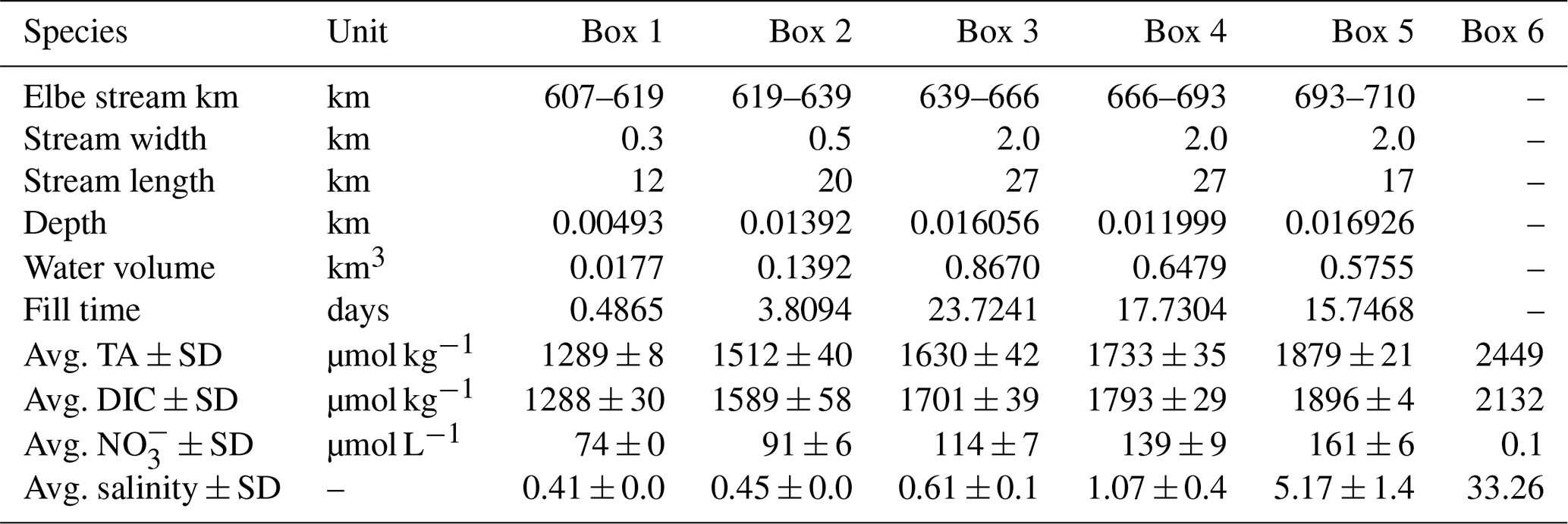
Located in the northern part of Germany, the Elbe Estuary extends approximately 140 km (Fig. 1), encompasses an area that begins at the weir in Geesthacht (Elbe stream km 586), crosses the port of Hamburg (Elbe stream km 623), and discharges near Cuxhaven (Elbe stream km 727) into the North Sea. The North Sea is a semi-enclosed shelf sea of the eastern North Atlantic that influences the estuary with its strong tidal cycles. This results in a semi-diurnal tidal range of 3.6 m in the port of Hamburg (Amann et al., 2012), the third largest port in Europe, and provides a continuous exchange of freshwater and marine water. The Elbe has an average annual long-term discharge of 704 m³ s⁻¹, measured at the last tide-free long-term sampling station in Neu Darchau (Elbe stream km 536) (Amann et al., 2012). Water depth in the Elbe Estuary is around 15–20 m but sharply decreases to 5 m upstream of Elbe stream km 620 (Hamburg port). For mass balance calculations, we separated the Elbe Estuary in six boxes, indicated by the lines in Fig. 1, of which box 1 (upstream of the Hamburg port) and box 6 (North Sea) act as boundary conditions.

Figure 1 Study site. The Elbe Estuary with sampling stations in June 2019 (dots) and the spatial separation of the estuary for the mass balance calculation (lines), whereby box 2 indicates the port of Hamburg in the upper estuary, box 3 and box 4 the middle estuary, and box 5 the lower estuary.

2.2 Sampling

This study is based on samples that we collected during a cruise (LP20190603) on RV Ludwig Prandtl on 2 consecutive days in June 2019 during ebb tide. We sampled from the German Bight around the island of Scharhörn upstream of Oortkaten situated in the riverine part of the estuary (Fig. 1). Discrete surface water (1.2 m depth) samples were collected every 20 min from a bypass of the flow-through FerryBox system (Petersen et al., 2011). Concurrently, the FerryBox provided the required physical parameters such as salinity, temperature, and oxygen.

First, water samples for total alkalinity (TA) and dissolved inorganic carbon (DIC) measurements were filled into 300 mL BOD (biological oxygen demand) bottles and preserved with 300 µL saturated mercury chloride (HgCl₂) to stop biological activity. The bottles, which are free of air bubbles, were then sealed with ground-glass stoppers coated in Apiezon^® type M grease and protected against opening by plastic caps. Samples were stored in a cool place in the dark until measured.

Samples for nutrients and stable isotopes of nitrate (NO${}_{\mathrm{3}}^{-}$) were collected to measure the concentration and the isotopic composition of nitrate, respectively. We collected three 15 mL Falcon tubes for triplicate nutrient measurement, and one 100 mL PE bottle (acid-washed overnight with 10 % HCl) for stable isotope analysis. Samples were filtered through pre-combusted GF/F filters and then frozen for onshore analyses.

We used pre-combusted (4 h, 450 ^∘C) GF/F filters to sample for particulate inorganic carbon (PIC) and particulate organic carbon and nitrogen (POC, PON) concentrations that we stored frozen until onshore analysis.

2.3 Analytical procedures

2.3.1 TA and DIC

We performed the TA and DIC measurements at Helmholtz-Zentrum Hereon using a VINDTA 3C (Versatile INstrument for the Determination of Total dissolved inorganic carbon and Alkalinity; MARIANDA – marine analytics and data). VINDTA 3C measures TA by potentiometric titration and DIC by coulometric titration (Shadwick et al., 2011). We used Certified Reference Material (CRM batch # 187) provided by Andrew G. Dickson (Scripps Institution of Oceanography) to calibrate TA and DIC measurements and ensured a precision of ± 2 µmol kg⁻¹.

2.3.2 Nutrients and stable nitrate isotopes

In order to determine nutrients, we used a continuous flow automated nutrient analyzer (AA3, SEAL Analytical) with a standard colorimetric technique (Hansen and Koroleff, 2007) to measure concentrations of dissolved nitrate (NO${}_{\mathrm{3}}^{-}$), nitrite (NO${}_{\mathrm{2}}^{-}$), and phosphate (PO${}_{\mathrm{4}}^{\mathrm{3}-}$). In order to measure ammonium (NH${}_{\mathrm{4}}^{+}$), we used a fluorometric method (Kérouel and Aminot, 1997). All samples were measured in triplicate.

We applied the denitrifier method (Casciotti et al., 2002; Sigman et al., 2001) to determine the stable isotope ratios of δ¹⁵N and δ¹⁸O of nitrate. By using denitrifying Pseudomonas aureofaciens (ATCC#13985), which lacks nitrous oxide reductase activity to reduce nitrate and nitrite in the filtered water sample to nitrous oxide (N₂O), we were able to measure the produced N₂O by a GasBench II coupled to an isotope mass spectrometer (Delta Plus XP, Fisher Scientific). Concurrently, we used two international standards (USGS34, δ¹⁵N-NO${}_{\mathrm{3}}^{-}=-\mathrm{1.8}$ ‰, δ¹⁸O-NO${}_{\mathrm{3}}^{-}=-\mathrm{27.9}$ ‰; IAEA, δ¹⁵N-NO${}_{\mathrm{3}}^{-}=+\mathrm{4.7}$ ‰, δ¹⁸O-NO${}_{\mathrm{3}}^{-}=+\mathrm{25.6}$ ‰) and one internal standard (δ¹⁵N-NO${}_{\mathrm{3}}^{-}=+\mathrm{7.6}$ ‰, δ¹⁸O-NO${}_{\mathrm{3}}^{-}=+\mathrm{24.4}$ ‰) for data correction in each run. The standard deviation for standards and samples was < 0.2 ‰ (n=4) for δ¹⁵N-NO${}_{\mathrm{3}}^{-}$ and < 0.5 ‰ (n=4) δ¹⁸O-NO${}_{\mathrm{3}}^{-}$. The nitrite concentration of the samples was usually less than 5 %, but when it exceeded this threshold, nitrite in the samples was removed with sulfamic acid (4 % sulfamic acid in 10 % HCl) prior to analysis (Granger and Sigman, 2009).

Variations in the natural abundance of stable isotopes are represented as relative differences in isotope ratios. The isotope ratio R is the ratio of heavy to light isotopes. Since isotope differences are very small, the delta-δ notation is used to describe the isotopic composition of samples (Eq. 1). Therefore, the isotopic ratio of a sample (R_sample) is given relative to the ratio of an internationally accepted reference material (R_reference). For this study, atmospheric N₂ and Vienna Standard Mean Ocean Water (VSMOW) are the reference materials for nitrogen and oxygen, respectively. The delta-δ notation is calculated as follows:

$$\begin{array}{}\text{(1)}& \mathit{\delta }\left(\mathrm{‰}\right)=\left({\displaystyle \frac{R_{\mathrm{sample}}-R_{\mathrm{reference}}}{R_{\mathrm{reference}}}}\right)\times \mathrm{1000}.\end{array}$$

We identified the nitrate sources upstream from the minimum isotope values at Elbe stream km 705 using Eq. (2). Here, we focused on the upper freshwater part of the estuary to identify the isotope values and the source of the additional nitrate (δ_ad) added to the estuary between Elbe stream km 609 and km 705. To investigate this further, we employed a simple mixing model (Sanders et al., 2018) with the δ¹⁵N and δ¹⁸O values and associated nitrate concentrations (C):

$$\begin{array}{}\text{(2)}& {\mathit{\delta }}_{\mathrm{ad}}={\displaystyle \frac{\left(\left({\mathit{\delta }}_{\mathrm{705}}x{C}_{\mathrm{705}}\right)-\left({\mathit{\delta }}_{\mathrm{609}}x{C}_{\mathrm{609}}\right)\right)}{\left(C_{\mathrm{705}}-C_{\mathrm{609}}\right)}}.\end{array}$$

2.3.3 Ancillary parameters

In order to determine POC and PON, the filters were measured for total carbon (TC) as a bulk sample first. Then, the filters were acidified three times with 1 N HCl and measured again for POC. The particulate inorganic carbon (PIC) was derived from the difference in carbon (C) content of the unacidified and acidified filters (TC-POC). The filters were measured with a CHN-elemental analyzer (Eurovector EA 3000, HEKAtech GmbH) in the Institute of Geology, University Hamburg, where the measurements were calibrated against the standards sulfanilamide (C=41.84 %, N=16.27 %) and acetanilide (C=71.09 %, N=10.36 %).

We directly measured the oxygen content with the FerryBox O₂ optode (Optode 3830, Aanderaa Instruments AS, Norway) (Petersen et al., 2011) and calibrated it with reference to parallel samples analyzed using the Winkler method.

The water depths that we used for the mass balances (see below) were measured during the cruise with the onboard acoustic Doppler current profiler (WorkHorse Broadband ADCP 1200 kHz, firmware version 51.40.) (Cysewski et al., 2018).

2.4 Gas flux calculation

As an input function for the mass balances (see below), we estimated CO₂ and O₂ gas exchange (F) between the atmosphere and water. We used the following equation:

$$\begin{array}{}\text{(3)}& F_{\mathrm{gas}}=k_{\mathrm{gas}}\times {\mathrm{\Delta }}_{\mathrm{gas}},\end{array}$$

where k_gas is the transfer velocity of the gases (O₂ and CO₂), and Δ_gas is the difference between the atmospheric and aquatic concentration, calculated as follows:

$$\begin{array}{}\text{(4)}& {\mathrm{\Delta }}_{\mathrm{gas}}={\left[\mathrm{gas}\right]}_{\mathrm{at}\mathrm{100}\mathrm{\%}\mathrm{saturation}}-{\left[\mathrm{gas}\right]}_{\mathrm{observed}}.\end{array}$$

The CO₂ concentration of the sample (observed) was computed from DIC, TA, salinity, and temperature using the CO₂SYS program by Lewis and Wallace (1998) and the dissociation constants for freshwater by Millero (1979). The CO₂ concentration of the sample corresponds to the mentioned pCO₂. The CO₂ concentration (at 100 % saturation) was obtained from TA and the global atmospheric CO₂ saturation of 416±0.13 µatm (Dlugokencky and Tans, 2021) by using the same previously mentioned program and constants.

We calculated the transfer velocity after Wanninkhof (2014) as follows:

$$\begin{array}{}\text{(5)}& k_{\mathrm{gas}}={\displaystyle \frac{\mathrm{0.251}\times {\left(U_{\mathrm{10}}\right)}^{\mathrm{2}}}{{\left(\frac{\mathit{\text{Sc}}}{{\mathit{\text{Sc}}}_{\mathrm{ref}}}\right)}^{-\mathrm{0.5}}}},\end{array}$$

where 0.251 is the coefficient of gas transfer, U₁₀ is the wind speed (in m s⁻¹) measured in situ at 10 m height by the federal authority Deutscher Wetterdienst (DWD) (provided by DWD, 2020), Sc is the Schmidt number, the kinematic viscosity of water divided by the diffusion coefficient of the gas (Wanninkhof, 2014), and Sc_ref is the Sc value relative to the reference conditions of the gas at 20 ^∘C in freshwater, which is 510 for O₂ and 600 for CO₂. The uncertainty of the flux calculation has been estimated to 20 % (Wanninkhof, 2014; Watson et al., 2009).

2.5 Mass balances

2.5.1 Box model approach

Based on our observations, we used a box model approach to balance the net dissolved budgets of TA, DIC, NO${}_{\mathrm{3}}^{-}$, and O₂ in the Elbe Estuary (Fig. 2). The box model approach allowed us to distinguish the conservative contributions from the marine and freshwater end-members based on salinity (i.e., baseline), the input and output values as advected transport, and the atmospheric gas exchange (O₂ and CO₂) of the observed parameters TA, DIC, NO${}_{\mathrm{3}}^{-}$, and O₂ between and within boxes. The resulting differences are the closing terms given as net dissolved budgets and referred to here as metabolic gains. To attribute the potential processes affecting metabolic generation, we distinguished between pelagic generation, which is associated with aerobic conditions – i.e., nitrification, which consumes TA – and benthic generation, which corresponds to anaerobic conditions, where anaerobic metabolic processes generate TA. We defined six boxes based on spatial and salinity considerations, with box 1 representing the freshwater (upstream of the Hamburg port) and box 6 the coastal ocean (North Sea) (Table 1). Both boxes 1 and 6 determined the start and end, were not balanced, and acted as boundary conditions. Calculation and end-member properties are shown in Table 1. Discharge per box was calculated using the observed depths, in combination with an average river discharge value (provided by FGG, 2021) measured from the last tide-free area at the long-term monitoring station Neu Darchau (Elbe stream km 536). Accordingly, we computed the fill time or, in other words, the freshwater flushing time of each box, as box volume divided by discharge (Table 1).

We used the following equation to calculate the metabolic gains by assuming a steady state:

$$\begin{array}{}\text{(6)}& \begin{array}{rl}{\displaystyle \frac{\mathit{\delta }\mathrm{C}}{\mathit{\delta }t}}& =\mathrm{0}=F_{\mathrm{Input}}+F_{\mathrm{Output}}+F_{\mathrm{Baseline}}\\ & +F_{\mathrm{ASF}\left({\mathrm{O}}_{\mathrm{2}},{\mathrm{CO}}_{\mathrm{2}}\right)}+F_{\mathrm{Metabolic}},\end{array}\end{array}$$

where F_Input is the input value, F_Output the output value, F_Baseline the salinity-corrected baseline value, $F_{\mathrm{ASF}({\mathrm{O}}_{\mathrm{2}},{\mathrm{CO}}_{\mathrm{2}})}$ the air–sea flux of O₂ and CO₂, respectively, and F_Metabolic the metabolic gain as the closing term.

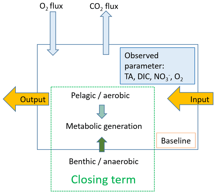
Figure 2 Schematic mass balance approach. We used a box model to balance the net dissolved budgets along the Elbe Estuary. The observed parameters are shown in light blue, and the closing term is set as metabolic generation (green), which is fueled by pelagic, i.e., aerobic, and benthic, i.e., anaerobic, processes but without allocating how much of what is generated where. The input and output is shown in yellow, and the latter acts as the input for the downstream box. To complete DIC and O₂, we included the atmospheric gas exchange. The baseline is calculated assuming conservative mixing of fresh and marine end-members.

Table 1 Elbe Estuary data for the mass balance calculation. The water depths were from an acoustic Doppler current profiler (ADCP) on board of RV Ludwig Prandtl, and the river length is based on the Elbe stream kilometer. The river width is based on measurements with Google Maps^®, while a standardized river width of 2 km was used for boxes 3, 4, and 5. The average river discharge on our sampling days was 423 m³ s⁻¹ (provided by FGG, 2021) measured at the last tide-free long-term sampling station in Neu Darchau (Elbe stream km 536). Average box values are given for total alkalinity (TA), dissolved inorganic carbon (DIC), nitrate (NO${}_{\mathrm{3}}^{-}$), and salinity. For the outer boundary conditions (box 6), we used a maximum salinity of 33.26, and respective TA (2449 µmol kg⁻¹), DIC (2132 µmol kg⁻¹), and NO${}_{\mathrm{3}}^{-}$ (0.1 µmol L⁻¹) values were taken on cruise HE541 (54.062456^∘ N, 8.015919^∘ E), which took place 2 months later in September 2019 and represent average summertime values for the German Bight. Standard deviation ± SD as spatial variability is given when possible.

The uncertainty of the closing term has been estimated by using the analytical measurement precision of 2 µmol kg⁻¹ for DIC and TA, 0.5 µmol L⁻¹ for NO${}_{\mathrm{3}}^{-}$, and 5 % for O₂ (Petersen et al., 2011). The gas exchange was considered with an uncertainty of 20 % (Wanninkhof, 2014; Watson et al., 2009). The river discharge uncertainty was 5 % (Léonard et al., 2000) and was added to the error in the end. The analytical measurement precision of POC and PON was 0.05 % and 0.005 %, respectively (Gaye et al., 2022), calculated from the average box 1 values. We calculated the analytical errors with the following equation per parameter and box:

$$\begin{array}{}\text{(7)}& X={\left({\sum }_{\mathrm{i}}{x}_{\mathrm{i}}^{\mathrm{2}}\right)}^{\mathrm{0.5}},\end{array}$$

where X is the combined error, and x_i are the errors of the individual observations.

2.5.2 TA source attribution

In order to assess the TA gains throughout Elbe Estuary, we compared the mass balance gains with the measured riverine particulate organic matter (POM) properties. Therefore, we used the riverine PIC and POC concentrations that were imported to the Hamburg port, where they can be converted into DIC and other molecules due to various processes. PIC mainly consists of CaCO₃. Depending on the ambient saturation, it is converted into DIC and Ca²⁺ by dissolution or vice versa by precipitation.

By using the imported riverine PIC and POC, we derived the maximum amount of TA fueled by CaCO₃ dissolution as the source and estimated the remaining amount of PIC transported downstream.

In order to estimate the TA gain that can be fueled by CaCO₃ dissolution, we considered the observed metabolic DIC, the average imported PIC : TC (particulate inorganic carbon : total carbon) ratio (0.29 ± 0.05), and the TA : DIC ratio for CaCO₃ dissolution (2) (Chen and Wang, 1999). To get the remaining DIC generated by, for example, organic matter respiration (POC), we multiplied the metabolic DIC gain by 0.71 (1–0.29 = 0.71). To arrive at the corresponding TA that was not fueled by CaCO₃ dissolution, we subtracted the TA fueled by CaCO₃ dissolution from the entire metabolic TA gain. We performed all calculations per box.

To estimate the amount of PIC that is transported through the estuary but not used for TA generation by CaCO₃ dissolution, we used the imported PIC (multiplied by the ratio of 2) and subtracted the previously calculated corresponding TA. The following boxes then do not refer to the imported PIC but to the product of the previous box that corresponds to the unused transported PIC. In the case of negative values such as in box 4, we set the transported PIC in the following calculation to 0.

For the coupling of carbon and nitrogen, we used the imported PON to estimate the amount that is transported, unused, through the Elbe Estuary and to estimate whether or not riverine PON import is sufficient to generate NO${}_{\mathrm{3}}^{-}$ and TA.

For estimating the TA generation fueled by denitrification (that we attribute here to imported riverine PON), we calculated the amount of PON that is available for denitrification by subtracting the nitrified PON (i.e., entire estuarine metabolic NO${}_{\mathrm{3}}^{-}$ gain) of the imported PON (box 1). With the calculated PON available for denitrification, the ratio of TA : DIC resulting from denitrification (0.9) (Chen and Wang, 1999), and the entire TA gain that is not fueled by PIC, we calculated the possible TA gain from PON that could be generated in the estuary without the occurrence of nitrification.

To estimate the amount of PON that can be transported downstream, we used the imported PON, the sum of the NO${}_{\mathrm{3}}^{-}$ gain of the mass balances, the previously calculated TA gain that was not fueled by PIC, and the TA : DIC ratio (0.9) for denitrification. The following boxes then do not refer to the imported PON but to the product of the previous box. In the case of negative values such as in box 4, we set the transported PON in the following calculation to 0.

2.6 Biogeochemical simulations

For estimating the effects of metabolic-produced alkalinity in the estuary on the North Sea and the continental shelf, we applied the 3D-ECOHAM model (Schwichtenberg et al., 2020). Pätsch and Kühn (2008) first described the ECOHAM model domain for this study (see their Fig. 1). Meteorological forcing for both models was derived from the ERA5 reanalysis data set (Hersbach et al., 2020).

The physical parameters temperature, salinity, horizontal and vertical advection, and turbulent mixing were calculated using the hydrodynamic model HAMSOM (Backhaus, 1985). This is a baroclinic primitive equation model using the hydrostatic and Boussinesq approximations. Details are described by Backhaus and Hainbucher (1987) and Pohlmann (1996). We ran the hydrodynamic model prior to the biogeochemical part. We saved the daily result fields and ran the biogeochemical model in offline mode.

The relevant biogeochemical processes and their parameterizations have been detailed in Lorkowski et al. (2012). TA and DIC are computed prognostically. The pelagic biogeochemical part is driven by planktonic production and respiration, calcite formation and dissolution, pelagic and benthic degradation and remineralization, and also by atmospheric deposition of reactive nitrogen. All of these processes affect TA. The air–sea flux of CO₂ was calculated for the North Sea region between 51 and 59.5^∘ N according to Wanninkhof (2014).

We extracted the year 2001 from the simulation run 1979–2014 for the analysis in this paper. Four different scenarios (50 %, 86 %, 100 %, and 150 % TA load) were run, with the 100 % scenario being the reference scenario with full riverine TA and DIC input. In comparison, the 86 % scenario reflects river input without the metabolic alkalinity generation corresponding to our calculated metabolic TA generation of 14 % throughout the Elbe Estuary. We ran two other scenarios, one with a reduced TA load (50 %) and one with an increased TA load (150 %), for a broader comparison. We used daily data of freshwater fluxes from 254 rivers discharging into the North Sea (Große et al., 2017). We applied corresponding river load data of nutrients, organic matter, DIC, and TA.

3 Results and discussion

3.1 Salinity, TA, DIC, and nutrient distribution along the estuary

Along the Elbe Estuary transect, the salinity varied from 0.40 in the freshwater part (Elbe stream km 609–680) to 27.84 in marine waters in the German Bight. The strongest salinity gradient was observed between Elbe stream km 683 and km 715 (box 5, tidal front) with an increase of 10 (Fig. 3a). The limited influence of salinity in the freshwater part, visible in Fig. 3a, limited the clear subdivision of boxes 1 to 3 in Fig. 3b.

TA and DIC increased from the upper estuary (Elbe stream km 609) to the mouth of the estuary (Fig. 3a), where the lowest concentrations were found in Oortkaten (1281 µmol TA kg⁻¹ and 1256 µmol DIC kg⁻¹ at 0.41 salinity), and the highest were found around Scharhörn (2272 µmol TA kg⁻¹ and 2016 µmol DIC kg⁻¹ at 27.84 salinity). In marine and brackish waters of the Elbe Estuary, TA was higher than DIC, while in the freshwater part of the estuary, DIC was higher than TA. At a salinity of 6.96, TA and DIC were equal with 1922 µmol kg⁻¹. The strongest increase in TA was observed in the freshwater part, between Elbe stream km 609 and km 670 (Fig. 3a), while in the outer estuary, TA and DIC increased almost proportional to the salinity gradient without obvious biological impact (Fig. 3a, b).

Nitrate (NO${}_{\mathrm{3}}^{-}$) concentrations increased from 73 µmol NO${}_{\mathrm{3}}^{-}$ L⁻¹ near Oortkaten to a maximum of 165 µmol NO${}_{\mathrm{3}}^{-}$ L⁻¹ in the lower estuary at a salinity of 5.08 (Elbe stream km 705, box 5) (Fig. 3a), which is downstream of the maximum turbidity zone (MTZ is located between Elbe stream km 664–670, not shown). Further downstream, nitrate mixed conservatively with low-NO${}_{\mathrm{3}}^{-}$ seawater to 15 µmol NO${}_{\mathrm{3}}^{-}$ L⁻¹ at km 750.

Ammonium (NH${}_{\mathrm{4}}^{+}$) reached a pronounced maximum of 15 µmol NH${}_{\mathrm{4}}^{+}$ L⁻¹ in the Hamburg port area, located upstream of the NO${}_{\mathrm{3}}^{-}$ maximum, while varying in a range around 1 µmol NH${}_{\mathrm{4}}^{+}$ L⁻¹ in the remainder of the estuary (Fig. 3a). This maximum coincides with the strongest gradients in DIC and TA and can be attributed to high remineralization rates in the port area, as is also evident by the high apparent oxygen utilization (AOU) (Fig. 3a).

Phosphate (PO${}_{\mathrm{4}}^{\mathrm{3}-}$) trends are comparable to nitrate, where a sharp increase in concentration is seen in the Hamburg port area and a maximum concentration of 2 µmol PO${}_{\mathrm{4}}^{\mathrm{3}-}$ L⁻¹ in the lower estuary (box 5), coinciding with the TA and DIC trend.

The δ¹⁵N-NO${}_{\mathrm{3}}^{-}$ and δ¹⁸O-NO${}_{\mathrm{3}}^{-}$ isotopic values were found to be higher in the upper estuary and decreased downstream to their respective minima at km 705, coinciding with the NO${}_{\mathrm{3}}^{-}$ maximum. In the freshwater part, the δ¹⁵N and δ¹⁸O values ranged from 12.4 ‰ to 17.1 ‰ and from 5.1 ‰ to 9.1 ‰, respectively.

The δ¹⁵N values of suspended particulate matter (SPM) (δ¹⁵N_p) showed a pronounced increase from 6 ‰ to 10 ‰ in box 2, indicating an enrichment of heavy isotopes in the particulate matter due to the degradation of POM. This strong increase coincides with the ammonium peak and the declining δ¹⁵N-NO${}_{\mathrm{3}}^{-}$.

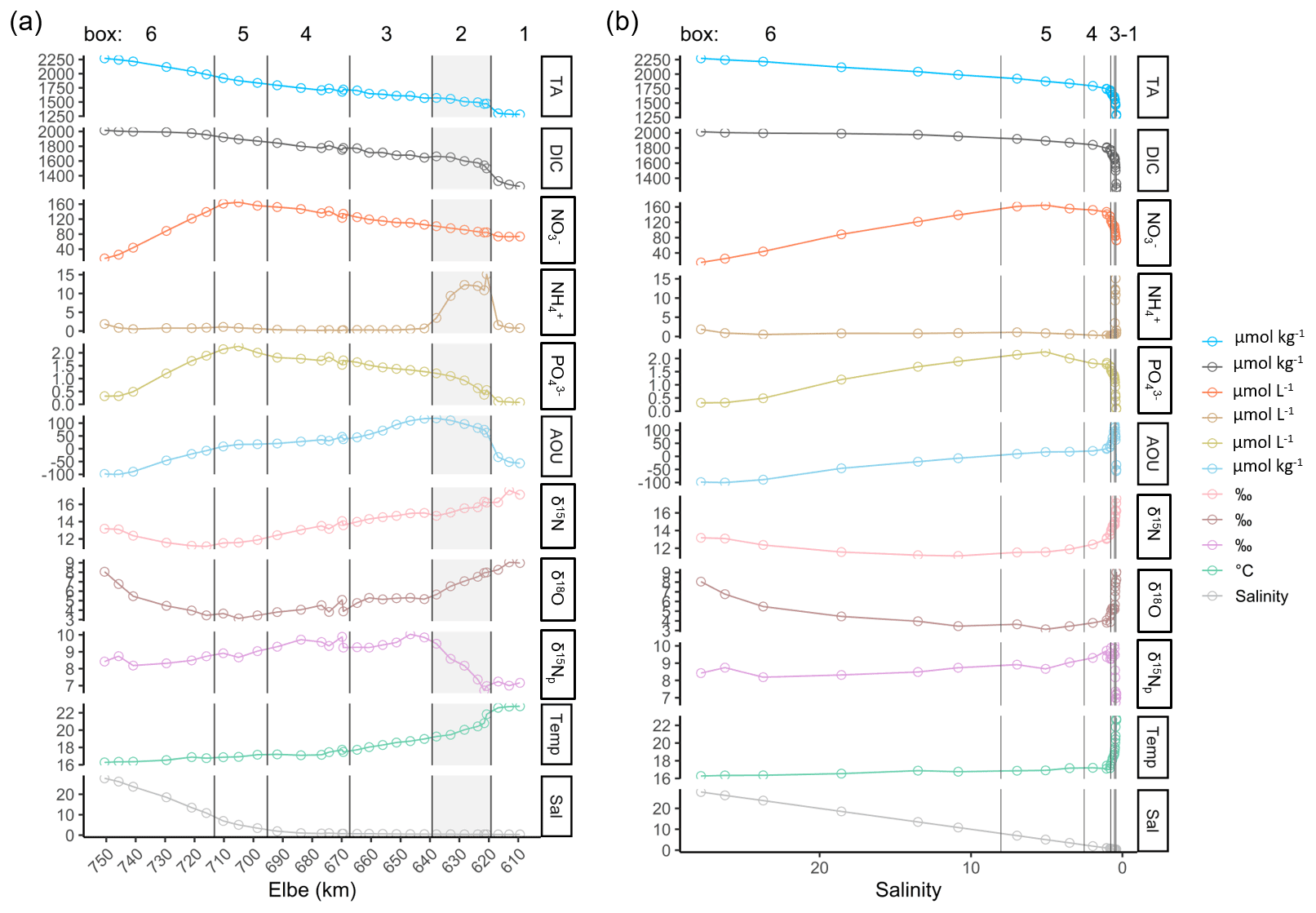
Figure 3 Spatial- and salinity-dependent observed parameter distribution along the Elbe Estuary. The data are from 2 d in June 2019. (a) Spatial observed parameter distribution from the inner estuary (Elbe stream km 609, right side) to the German Bight around the island of Scharhörn (computed Elbe stream km 750, left side). Total alkalinity (TA), dissolved inorganic carbon (DIC), nitrate (NO${}_{\mathrm{3}}^{-})$, ammonium (NH${}_{\mathrm{4}}^{+})$, phosphate (PO${}_{\mathrm{4}}^{\mathrm{3}-})$, apparent oxygen utilization (AOU), and delta values of nitrate isotopes (δ¹⁵N, δ¹⁸O), of filtered water, and of suspended particulate matter (δ¹⁵N_p), as well as temperature (Temp; in ^∘C) and salinity (Sal), are shown. The vertical lines indicate the designated boxes for the mass balance calculation, in which the inner boundary (box 1) is on the right side of the plot, followed by the shaded box 2 with the Hamburg port area (upper estuary), boxes 3 and 4 (middle estuary), box 5 (lower estuary), and the outer marine boundary (box 6) on the left side of the plot. (b) Salinity-dependent observed parameter distribution. Note the different y-axis scales within the different panels of both plots.

3.2 Metabolic activity in the port

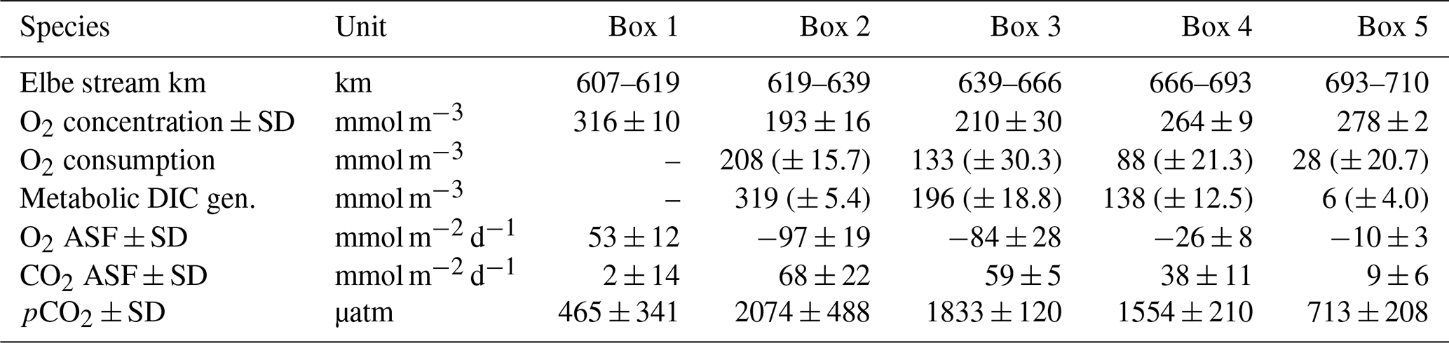
The North Sea's carbonate system is affected by the surrounding coastal areas (Schwichtenberg et al., 2020), necessitating a specific investigation of estuarine-based TA generation and an estimation of its impact on the oceanic CO₂ uptake capacity. In order to determine the TA-, DIC-, and O₂-related metabolic activity in the Elbe Estuary, we estimated the air–sea gas exchange of CO₂ and O₂, as these are non-advective processes along the Elbe Estuary (Fig. 4a, Table 2). Upstream of the port of Hamburg, the pCO₂ was slightly supersaturated (465 µatm) relative to the atmosphere (416 µatm). Within the Hamburg port, the highest pCO₂ values (2074 µatm) were recorded, indicating strong CO₂ degassing, while further downstream, the pCO₂ decreased again (Table 2). In other European estuaries a similar pCO₂ pattern has been recorded (Frankignoulle et al., 1998). Lastly, taking into account the pO₂, which mirrored the pCO₂ evolution along the estuary, we could estimate respective sea to air (in the case of CO₂) and air to sea (in the case of O₂) fluxes (Fig. 4a).

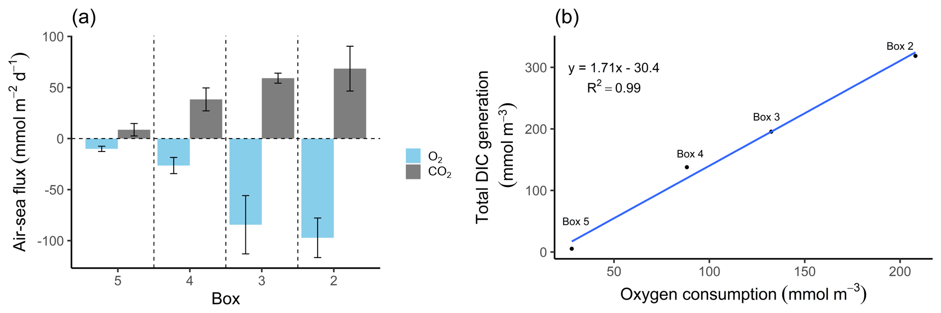
Figure 4 O₂ and CO₂ characteristics. (a) Air–sea fluxes (ASFs) of oxygen (O₂) and carbon dioxide (CO₂) per box. The O₂ ASFs were calculated from pO₂ and observed oxygen concentrations, and the CO₂ ASFs were calculated from pCO₂ values and observed TA (Table 2). Values are shown with standard deviation represented as spatial variability (error bars). Positive values indicate outgassing, while negative values indicate a gas uptake into the water. The Hamburg port area is located in box 2 and the lower estuary in box 5. (b) Relationship between metabolic DIC generation and O₂ consumption along the estuary in concentration (mmol m⁻³). Please note the different parameters in the panels.

Table 2 Average calculated gas values per box. O₂ concentration is the observed oxygen. O₂ consumption is the amount of oxygen consumed (i.e., AOU + oxygen uptake). Metabolic DIC gen. is the generated DIC. O₂ ASF is the oxygen, and CO₂ ASF is the carbon dioxide air–sea flux along the surface. Positive flux values indicate outgassing, while negative values indicate an absorption into the water. pCO₂ is the partial pressure of carbon dioxide and corresponds to the CO₂ concentration in the water. The standard deviation ± SD as spatial variability is given when possible. An uncertainty estimation including the uncertainties of the analytical measurements, the air–sea flux estimation, and the river discharge is given as (± absolute errors) by an error propagation (Methods).

The highest metabolic DIC generation and O₂ consumption (Fig. 4a, b, Table 2) occurred in the port of Hamburg, where most of the CO₂ produced remained dissolved, with only a moderate amount being emitted to the atmosphere. The strong metabolic activity is also reflected by the high oxygen influx, driven by low-oxygen conditions in the port of Hamburg (Table 2; see, for example, Amann et al., 2012; Schöl et al., 2014). In Fig. 4b, the high slope of 1.71 of DIC and O₂ exceeds the ratio of 0.5 to 1 (e.g., Thomas, 2002), indicating anaerobic or particulate inorganic DIC sources. This therefore suggests that the remnants of the high metabolic activity in box 2 are transported further downstream, eventually approaching an equilibrium within the lower estuary (box 5; Fig. 4a, b). Accordingly, there the observed metabolic values obtained for DIC (Fig. 5) and O₂ (AOU; Fig. 3) are to a large degree advected signals. Using the mass balances, we calculated the net dissolved budgets of TA, DIC, and NO${}_{\mathrm{3}}^{-}$, where only the net gains were represented but there is no indication of what processes were responsible for it. The highest metabolic gains of both TA and DIC were found in the Hamburg port area (box 2), identifying this area as having the highest metabolic activity (Fig. 5), almost an order of magnitude larger than that found in the downstream boxes. Accordingly, very high metabolic fluxes, i.e., area- and time-normalized values, of TA (808 mmol m⁻² d⁻¹) and DIC (1164 mmol m⁻² d⁻¹) were obtained for the Hamburg port area (box 2) (Fig. 5, Table 3). Downstream of the Hamburg port, values below 150 mmol m⁻² d⁻¹ and decreasing toward the North Sea were found, with negligible values in box 5. Similarly, the contribution of metabolically generated DIC is higher in the port area than downstream, where CO₂ equilibration with the atmosphere gains (relative) importance. Compared to the metabolic gains, the air–sea flux (ASF) constitutes only a minor fraction of the metabolic fluxes (Fig. 5). The high release of DIC relative to TA (Fig. 5) is in line with our above result of high pCO₂ in box 2 (Fig. 4a).

In contrast to TA and DIC, the metabolic NO${}_{\mathrm{3}}^{-}$ fluxes have a similar magnitude along the estuary, with the highest fluxes (63 mmol m⁻² d⁻¹) in the port of Hamburg and lower fluxes (between 16 and 21 mmol m⁻² d⁻¹) in the downstream parts of the estuary. Nevertheless, compared to TA and DIC, the relative difference between box 2 and the downstream boxes is much smaller for NO${}_{\mathrm{3}}^{-}$ (Fig. 5).

For the entire Elbe Estuary, we estimated the total dissolved metabolic DIC and TA loads from all boxes released into the North Sea (excluding the air–sea fluxes). Our calculations yield annual metabolic loads of 5.6 Gmol yr⁻¹ for TA and 6.5 Gmol yr⁻¹ for DIC. In relation to the most recent data from 2017 (Pätsch and Lenhart, 2019), these metabolic loads represent 16 % of the overall Elbe DIC (39.6 Gmol DIC yr¹) and 14 % of the overall TA (40.3 Gmol TA yr¹) loads.

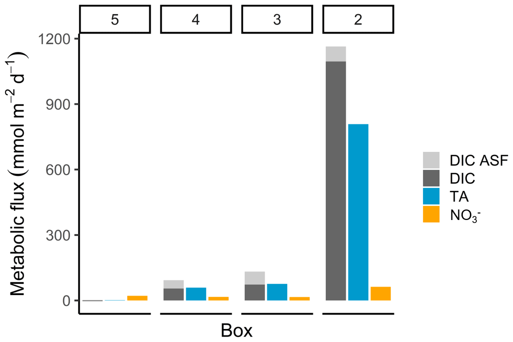
Figure 5 Metabolic fluxes of total alkalinity, dissolved inorganic carbon, and nitrate. The metabolic fluxes of TA (blue), DIC (dark grey), and NO${}_{\mathrm{3}}^{-}$ (orange; in mmol m⁻² d⁻¹) are shown, with the additional visualization of the air–sea flux (ASF) contribution to DIC (light grey) to demonstrate the entire generation and their relative magnitude.

3.3 Carbon-based constraints on TA generation

In order to explain the net total alkalinity gains generated in the Elbe Estuary that were identified with the mass balances, we compared them to imported riverine particulate organic matter (POM) properties from samples taken simultaneously to our Elbe transect (Table 3). Natural variability, such as seasonality, may change the imports and lead to modified amounts of TA generation by the different processes.

Here, we used imported riverine particulate inorganic and organic carbon (PIC, POC) properties to attribute the TA gain fueled by calcium carbonate (CaCO₃) dissolution and to estimate the remaining PIC amount that is transported downstream to identify a possible CaCO₃ deficit along the estuary.

We obtained TA generation from CaCO₃ dissolution referring to the metabolic, i.e., POM-driven, DIC generation multiplied by the observed PIC : TC ratio of 0.29 ± 0.05 (average of entire estuary) of the imported POM. We assumed spontaneous, i.e., maximum, dissolution of CaCO₃, which integrated over the estuary, can contribute up to 90 % of the TA generation and can be considered as an upper bound. This result can be supported by the studies of Kempe (1982) and Francescangeli et al. (2021), who report undersaturated calcite saturation states (Ω) in the upper estuary and at their most freshwater station in the middle estuary.

Our estimate should be considered an upper bound, since other anaerobic metabolic processes must provide the remaining at least 10 % of the generated TA we observed. However, our data set does not allow us to directly identify or even quantify any of these processes, nor does it allow us to exclude them.

In order to estimate the contribution of denitrification as a source for TA generation in the Elbe Estuary and to shed further light on the coupling between TA and nitrogen cycles, we related imported riverine particulate organic nitrogen (PON) to metabolically released NO${}_{\mathrm{3}}^{-}$.

Without NO${}_{\mathrm{3}}^{-}$ generation by nitrification, we could explain TA generation by denitrification with around 9 % of the overall metabolic TA gain. However, under consideration of both processes occurring in the estuary, we were unable to further attribute denitrification as the entire source for the TA generation in the Elbe Estuary. We identified a nitrogen deficit of riverine-imported PON to fuel both NO${}_{\mathrm{3}}^{-}$ generation (i.e., by nitrification) and TA generation (i.e., by denitrification) in boxes 4 and 5 (Table 3) that affects the balance of the entire estuary. This in turn means that lateral NO${}_{\mathrm{3}}^{-}$ sources need to be inferred to balance the nitrogen budget. Similarly, there is fairly constant NO${}_{\mathrm{3}}^{-}$ gain along the estuary (Fig. 5), but both decreasing O₂ consumption and DIC generation downstream (Figs. 4b, 5) imply a surplus of nitrate in the downstream part, thus a decoupling between carbon and nitrogen cycling.

To provide further evidence for lateral NO${}_{\mathrm{3}}^{-}$ sources (Kendall et al., 2007; Middelburg and Nieuwenhuize, 2001; Sigman et al., 2001), we employed nitrate stable isotope (δ¹⁵N, δ¹⁸O) signatures. Similar to Dähnke et al. (2008), minimum δ¹⁵N and δ¹⁸O values were found in the section with maximum observed NO${}_{\mathrm{3}}^{-}$ concentrations (box 5). The minima were lower than would be expected based on conservative mixing of North Sea and riverine end-members, as well as from nitrification processes, during the 10–30 d downstream transport of waters (see, for example, Spieckermann et al., 2021) (Fig. 3a). Nitrification preferentially releases lighter nitrate, depending on the sources for nitrification as evidenced by both decreasing δ¹⁵N values in NO${}_{\mathrm{3}}^{-}$ and increasing δ¹⁵N values in SPM (Fig. 3a), but cannot explain the observed local minimum alone. The minimum in isotopic signature is in line with assumed delta values of the added nitrate (Eq. 2) of 7.1 ‰ for δ¹⁵N-NO${}_{\mathrm{3}}^{-}$ and −1.6 ‰ for δ¹⁸O-NO${}_{\mathrm{3}}^{-}$ (Table 4), which in turn points to an allochthonous, lateral nitrate source. Such can be fueled by soil ammonium oxidation, manure, and septic waste (Kendall et al., 2007), which can be identified as nitrogen sources with sufficiently light δ¹⁵N and δ¹⁸O characteristics. Although our study implies a lateral NO${}_{\mathrm{3}}^{-}$ source, in contrast to earlier studies (Dähnke et al., 2008; Sanders et al., 2018), we cannot elucidate the corresponding source processes and regions in the context of this study.

Within the entire estuary, the spatial distributions of NO${}_{\mathrm{3}}^{-}$ gain on one hand and the O₂ consumption and metabolic DIC generation on the other hand show incoherent patterns. We found a decoupling of carbon, nitrogen, and oxygen in the middle and lower estuary, with a fairly constant NO${}_{\mathrm{3}}^{-}$ gain along the estuary (Fig. 5) but both decreasing O₂ consumption and DIC generation river downstream (Figs. 4b, 5). Thus, neither O₂ nor DIC reflects the NO${}_{\mathrm{3}}^{-}$ gain, suggesting additional nitrate sources in the downstream freshwater part of the estuary.

Accordingly, estuarine ecosystems appear to be highly susceptible to nutrient management actions that affect the balance of the various metabolic processes that generate TA by controlling NO${}_{\mathrm{3}}^{-}$ availability, as organic carbon and oxygen supply appear in excess or steady, respectively. One could speculate that the reduced organic carbon supply would reduce the importance of anaerobic processes in favor of a relative increase in aerobic respiration. On the other hand, a reduction in NO${}_{\mathrm{3}}^{-}$ for a given organic carbon content would trigger other anaerobic processes (e.g., iron or sulfate reduction) that have a higher TA gain per unit of carbon respired than denitrification does (Chen and Wang, 1999).

Table 3 Mass balance results and POM properties. The mass balance results are shown as metabolic generation (i.e., gains) in concentrations (mmol m⁻³), in fluxes of total alkalinity (TA), dissolved inorganic carbon (DIC), and nitrate (NO${}_{\mathrm{3}}^{-}$), respectively (metabolic fluxes are also visualized in Fig. 5), and in kilomoles per day (kmol d⁻¹). The average carbon : nitrogen (C : N) and particulate inorganic carbon : total carbon (PIC : TC) ratios of suspended particulate matter (SPM) are given per box. The observed imported POC and particulate organic nitrogen (PON) values based on sampled filters in box 1, as well as the calculated transported values for PON in the other boxes (2–5) (Sect. 2.3), are shown. Imported PIC for box 1 was calculated based on imported POC, and transported PIC values were calculated for the other boxes (2–5) (Sect. 2.3). DIC fueled by PIC and TA fueled by PIC give the amount of each that can be fueled by imported and transported PIC. DIC not fueled by PIC and TA not fueled by PIC give the amount of each that is remaining and not fueled by imported PIC, i.e., CaCO₃ dissolution. The standard deviation ± SD as spatial variability is given when possible. An uncertainty estimation for analytical measurements, the air–sea flux estimation, and the river discharge is given as (± absolute errors) by an error propagation (Sect. 2.3). Imported POC, PIC, and PON to the estuary were estimated using measured average POC (596 ± 52 µmol L⁻¹) and PON (91 ± 8 µmol L⁻¹) concentrations of SPM (47 ± 5 mg L⁻¹), all determined for box 1. PIC is here a synonym for CaCO₃ dissolution as source.

Table 4 Added nitrate values. The initial values and the changes in the nitrate concentration (µmol L⁻¹) and the associated stable isotopes (δ values in ‰) between Elbe stream km 609 and km 705 are shown.

3.4 Estuarine carbon release and estimated impact on coastal carbon storage

The impacts of anthropogenic and management activities on estuarine and coastal carbon cycling, as well as CO₂ uptake, have frequently been discussed from an aerobic perspective, as, for example, by Borges and Gypens (2010) for the southern North Sea. Here we attempt to complement this perspective by considering anaerobic processes. We employed a biogeochemical simulation approach (Schwichtenberg et al., 2020) to estimate the impacts of estuarine metabolic TA gains on the carbon cycle and CO₂ uptake capacity in the North Sea. We used this simulation approach to highlight the effect of changing DIC : TA ratios, e.g., due to anthropogenic-induced changes, on the carbon storage in coastal oceans. Conceptually, the simulations reflect the relative balance between aerobic and anaerobic respiration of a given amount of organic carbon such that any reduced alkalinity scenario returns a preference for aerobic processes, and the increased alkalinity scenarios in turn imply a preference of anaerobic processes releasing a given amount of DIC. We applied four scenarios in which we changed the TA loads as the input variable and compared the resulting CO₂ uptake by the North Sea at three different distances from coast. For the first scenario, the reference run (i.e., normal conditions), we used the full riverine TA and DIC load that corresponds to a TA load of 100 %. For the second scenario, we reduced the TA load to 86 % reflecting the above contribution (14 %) of metabolic alkalinity to the overall alkalinity release by the Elbe Estuary. For further comparisons, we ran scenarios with a reduced TA load to 50 % and an increased TA load to 150 %. We extrapolated these scenarios to 254 rivers that discharge into the North Sea. Especially the major rivers and estuaries are either associated with a major port (e.g., Antwerp, Rotterdam, London, or Bremerhaven) or generally characterized as a highly turbid and heavily used waterway (e.g., Ems) that, like the Elbe Estuary, provide ideal conditions for anaerobic metabolic pathways.

Under reference conditions (100 % TA), the open North Sea (>200 km distance from the coastline) absorbs more atmospheric CO₂, with carbon transported in the deeper zones via the continental shelf pump (Thomas et al., 2004), than the coastal zones (100 km distance) (Fig. 6, absolute ASF indicated by bars). This spatial distribution is also visible in the scenarios with reduced TA loads. Assuming a remaining TA load of 50 % and 86 %, we modeled less CO₂ uptake due to reduced metabolic alkalinity generations.

Compared to the reduced TA scenarios, the increased TA scenario (150 %) also has higher CO₂ uptake within each distance but, in spatial distribution, higher CO₂ uptake in coastal areas than in the open North Sea. This indicates that in the 150 % scenario the open North Sea no longer represents the area of strongest CO₂ uptake.

The differences in CO₂ uptake in the North Sea (Fig. 6, difference ASF indicated by lines) between the scenarios with reduced TA (50 % and 86 %) and the reference scenario (100 %) decreased with increasing distance from the coast. This change is also reflected in the difference in CO₂ uptake between the scenario with increased TA load (150 %) and the reference scenario, where the difference in CO₂ uptake is higher in the coastal area than in the open ocean. This phenomenon can be partly explained by mixing, as the signal is more diluted further off shore. Furthermore, CO₂ equilibration continues as waters are transported offshore (e.g., Burt et al., 2014), i.e., away from the TA source. The larger differences in CO₂ uptake in coastal areas suggest that the effects of TA input from metabolic processes in rivers are similar in magnitude to the simulated (Fig. 6) and observed (Thomas et al., 2004) air–sea flux itself. Similar evidence has been presented by Burt et al. (2016), who report that benthic sediment release in the southern North Sea shapes, if not dominates, the seasonal variability in the TA system (see also Thomas et al., 2009).

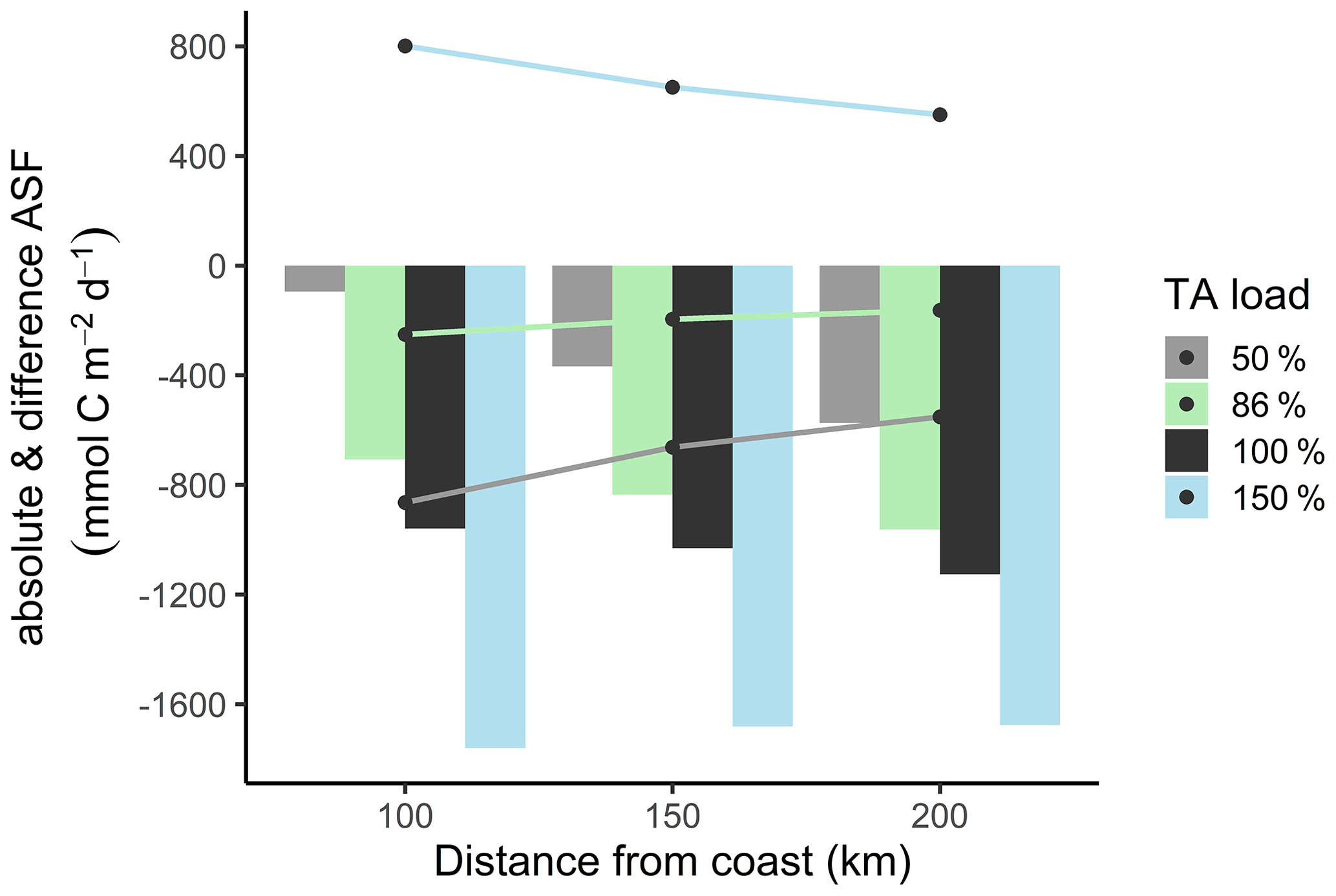
Figure 6 Biogeochemical CO₂ air–sea flux (ASF) simulations at distance from coast. The bars show the annual absolute CO₂ uptake in the water under reduced (50 %, grey; 86 %, green), normal (100 %, black), and increased (150 %, blue) TA load. The lines visualize the CO₂ uptake difference between the 50 %, 86 %, and 150 % scenarios and the reference scenario (100 %).

Next to CO₂ air–sea fluxes, the metabolic TA release from the Hamburg port area could also affect calcifying organisms such as foraminifera that occur in the lower Elbe Estuary. In a recent study, Francescangeli et al. (2021) observed the change in calcite saturation state (Ω_Ca) from under- to supersaturation around Elbe km 685 (approx.). Without the respective TA generation, the supersaturated range and thus the habitat of the foraminifera would clearly be further downstream, if not restricted to the North Sea. For example, at their most saline station (Francescangeli et al., 2021, see their Fig. 2f), corresponding to Elbe stream km 730 in our study, the observed Ω_Ca is ∼ 3.3, whereas it would be strongly undersaturated (Ω_Ca ∼ 0.2) without benthic TA release.

4 Conclusions

We observed clear regional differences in the biogeochemistry of the Elbe Estuary. While conservative mixing prevails in the salinity gradient of the lower estuary, metabolic processes dominate the upper, freshwater part within the port of Hamburg. We observed a strong increase of several hundred micromoles per kilogram of TA and DIC in the Hamburg port (Fig. 3) with diminishing values downstream and calculated an annual metabolic TA load of about 14 % of the total TA runoff from the Elbe River to the coastal ocean.

Mass balances suggest that up to 90 % of the generated TA of the entire estuary could be fueled by imported PIC, i.e., through CaCO₃ dissolution and that the remaining at least 10 % of the generated TA may be due to anaerobic metabolic processes such as denitrification, iron, manganese, or sulfate reduction. Nevertheless, the uncertainty of natural variabilities such as seasonality or extreme weather (e.g., dry or rain events) may exert control over relative and absolute occurrence of the above processes.

However, the interplay of the various metabolic processes governs both the release of reduced products and the carbonate system properties in the estuary. For example, the former controls the balance of released gases such as N₂, N₂O, and H₂S, which in turn can have negative effects on the entire estuarine biodiversity, leading to losses in reproduction and habitats of, for example, local fish species (Breitburg et al., 2009; Breitburg, 2002; Janas and Szaniawska, 1996; Wu, 2009). The carbonate system properties regulate the habitable range of, for example, benthic foraminifera (Francescangeli et al., 2021). We show that the metabolic TA release increases the capacity and CO₂ absorption in the German Bight. Compared to the open ocean, the coastal ocean would act as a stronger CO₂ sink with increased TA loads. We postulate that this result may be transferable to other global rivers or estuarine systems, particularly those with large port facilities, and that it could have tangible implications for the ocean's CO₂ uptake capacity on a global scale.