Using atmospheric observations to quantify annual biogenic carbon dioxide fluxes on the Alaska North Slope

The continued warming of the Arctic could release vast stores of carbon into the atmosphere from high-latitude ecosystems, especially from thawing permafrost. Increasing uptake of carbon dioxide (CO₂) by vegetation during longer growing seasons may partially offset such release of carbon. However, evidence of significant net annual release of carbon from site-level observations and model simulations across tundra ecosystems has been inconclusive. To address this knowledge gap, we combined top-down observations of atmospheric CO₂ concentration enhancements from aircraft and a tall tower, which integrate ecosystem exchange over large regions, with bottom-up observed CO₂ fluxes from tundra environments and found that the Alaska North Slope is not a consistent net source nor net sink of CO₂ to the atmosphere (ranging from −6 to +6 Tg C yr⁻¹ for 2012–2017). Our analysis suggests that significant biogenic CO₂ fluxes from unfrozen terrestrial soils, and likely inland waters, during the early cold season (September–December) are major factors in determining the net annual carbon balance of the North Slope, implying strong sensitivity to the rapidly warming freeze-up period. At the regional level, we find no evidence of the previously reported large late-cold-season (January–April) CO₂ emissions to the atmosphere during the study period. Despite the importance of the cold-season CO₂ emissions to the annual total, the interannual variability in the net CO₂ flux is driven by the variability in growing season fluxes. During the growing season, the regional net CO₂ flux is also highly sensitive to the distribution of tundra vegetation types throughout the North Slope. This study shows that quantification and characterization of year-round CO₂ fluxes from the heterogeneous terrestrial and aquatic ecosystems in the Arctic using both site-level and atmospheric observations are important to accurately project the Earth system response to future warming.

1 Introduction

The Arctic surface air temperature is warming at twice the rate of the global average (Box et al., 2019; Meredith et al., 2019). Continued thawing of Arctic permafrost has the potential to release vast stores of carbon into the atmosphere, thereby further accelerating warming (Schuur et al., 2015; Hugelius et al., 2014). In the biosphere, the net CO₂ flux is the balance between the uptake of CO₂ by vegetation through photosynthesis (negative net CO₂ flux indicates removal from the atmosphere) and the release of CO₂ into the atmosphere by plant and microbial respiration (positive net CO₂ flux indicates a source to the atmosphere). Arctic growing seasons are short (∼3 months), and the long cold season dominates the seasonal cycle. The transition between the growing and cold seasons is marked by the soil zero-curtain period, when belowground temperatures of the active layer above frozen permafrost remain near freezing; the active layer is insulated by snow and ice at the surface and warmed by the latent heat release of freezing water (Outcalt et al., 1990). During the zero-curtain period, soil respiration can remain active in deeper soils for weeks to months after the end of the growing season (Zona et al., 2016; Romanovsky and Osterkamp, 2000). As the climate warms, the active layer above permafrost deepens, thawed soils become wetter, a larger volume of soil remains unfrozen for a longer period of time, and the duration of the zero-curtain period plays an increasingly important role in determining the net carbon exchange in Arctic ecosystems (Kim et al., 2012; Arndt et al., 2019). Recent work has shown a significant cold-season source of CO₂ from Arctic ecosystems, including more than a 70 % increase in October–December CO₂ concentration enhancements in the past 40 years, consistent with an increase in cold-season respiration, which is not well represented in Earth system models (Commane et al., 2017; Natali and Watts et al., 2019). Neglecting these processes could lead to a large underestimation of CO₂ emissions, biassing current and future climate projections.

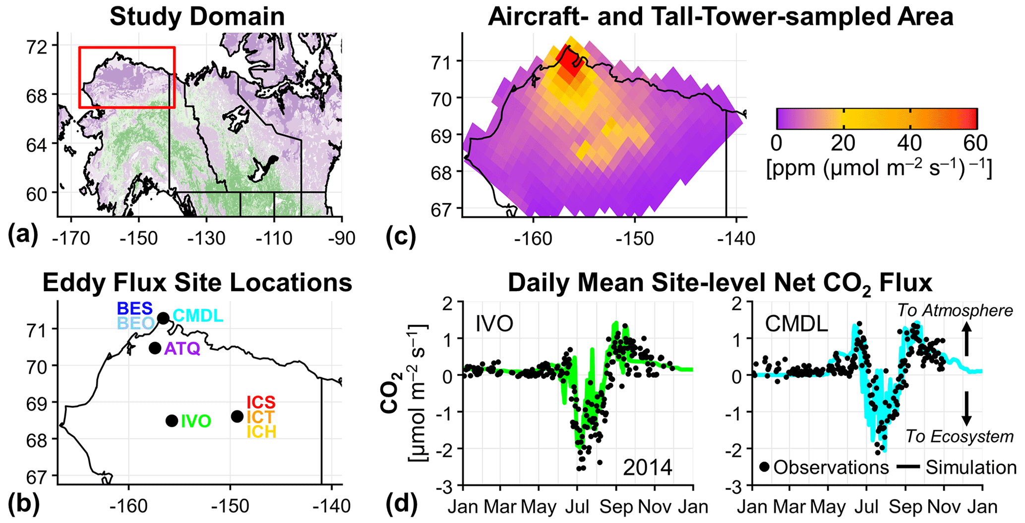
Figure 1 Alaska North Slope study region, eddy flux site locations, area sampled by aircraft and the tower, and example results from the eddy flux site measurement–model comparison. (a) North Slope region (red box) within Alaska and northwestern Canada; tundra areas are shown in purple, and boreal forest areas are shown in green (Luus et al., 2017). (b) Location of eddy flux measurement sites on the Alaska North Slope used in this analysis. (c) The 10 d WRF-STILT (Weather Research and Forecasting–Stochastic Time-Inverted Lagrangian Transport) footprints used to sample CO₂ flux models, summed for all aircraft and tall-tower CO₂ observations used in this analysis; colors represent values greater than 0 and are saturated at 60 $\mathrm{ppm}(\mathrm{\mu }\mathrm{mol}{\mathrm{m}}^{-\mathrm{2}}{\mathrm{s}}^{-\mathrm{1}}{)}^{-\mathrm{1}}$, and the maximum value near Utqiaġvik, Alaska, is 324 $\mathrm{ppm}(\mathrm{\mu }\mathrm{mol}{\mathrm{m}}^{-\mathrm{2}}{\mathrm{s}}^{-\mathrm{1}}{)}^{-\mathrm{1}}$. (d) Time series of the observed (black dots) and simulated (colored lines) site-level daily mean net CO₂ flux for 2014 at the Ivotuk (IVO; left) and Climate Monitoring and Diagnostics Laboratory (CMDL; right) eddy flux measurement sites, where site-level Tundra Vegetation Photosynthesis and Respiration Model (TVPRM) net CO₂ flux simulations are driven by North American Regional Reanalysis (NARR) meteorology and the solar-induced chlorophyll fluorescence (SIF) product from the contiguous SIF (CSIF) dataset. Positive net CO₂ flux values indicate CO₂ fluxes into the atmosphere throughout this study. A comparison for all eight eddy flux sites is provided in Fig. S1 in the Supplement.

Tundra ecosystems, characterized by frozen soils covered in low shrubs, sedges, grasses, and mosses, make up approximately 50 % of the Arctic landscape (Raynolds et al., 2019). Due to the lack of trees, the magnitude of net CO₂ uptake in tundra during the growing season is relatively small and may be offset by emissions from respiration that can continue well into the cold season (Watts et al., 2021). In the past, year-round CO₂ flux measurements from tundra ecosystems were rare due to difficulties in maintaining instrumentation under remote and extreme cold conditions (Euskirchen et al., 2017; Kittler et al., 2017; Goodrich et al., 2016). Long-term year-round CO₂ concentration measurements have been made in the Arctic at a small number of tall towers, which have been situated to sample clean marine air off the ocean (Jeong et al., 2018; Worthy et al., 2009). While aircraft provide greater spatial coverage over land than these towers, they tend to operate for short durations, and their temporal coverage is limited by weather and visibility during the cold season (Chang et al., 2014; Commane et al., 2017; Miller et al., 2016). However, the recent increase in the availability of observations of gas fluxes and concentrations within a particular tundra region, the Alaska North Slope (Fig. 1a), is making it possible to better conduct year-round multi-scale assessments of tundra ecosystems, with the aim of improving our understanding of CO₂ sink/source activity and carbon budgets in these environments.

Currently, observations and models do not agree on the sign of the annual net CO₂ flux across the Alaska North Slope region. Site-level measurements and atmospheric observations suggest that this region is a net CO₂ source (Commane et al., 2017; Oechel et al., 2014; Euskirchen et al., 2017). However, a comparison of process-based models of the North Slope found large variability in the sign and magnitude of the net CO₂ flux with an approximately neutral regional annual net CO₂ flux multi-model mean of $-\mathrm{3.5}\pm \mathrm{67}$ Tg C yr⁻¹ (Fisher et al., 2014). In a more recent study, Tao et al. (2021) found an annual net CO₂ flux range of −9 to 12 Tg C yr⁻¹ for the years 2010–2016, with only 2014 being an annual net CO₂ source. Extrapolating from site-level CO₂ flux measurements to regional budgets is difficult due to the extreme heterogeneity of tundra ecosystems in the North Slope region as well as a lack of spatial and seasonal representativeness by existing flux monitoring sites (Pallandt et al., 2022).

In this study, we compare bottom-up flux estimates with top-down atmospheric observations from aircraft and a tall tower using an integrated modeling approach to quantify the CO₂ budget sign and magnitude of the Alaska North Slope. Our framework first applies a bottom-up approach to understand Arctic tundra ecosystem CO₂ fluxes, constrained by site-level observations, using an empirical model ensemble of CO₂ fluxes derived from eddy flux measurements representing varied tundra ecosystems within the region. We then apply top-down information gained from regional CO₂ concentration enhancement observations measured by a tall tower and aircraft, which sample the atmosphere–biosphere exchange throughout the Alaska North Slope, to evaluate the range of potential CO₂ fluxes identified by the bottom-up model ensemble for 2012–2017. This evaluation also identifies the ecosystem parameterizations, vegetation distributions, and environmental drivers that best characterize the observed spatial and temporal distribution of biogenic CO₂ in the atmosphere across the region. By developing regional CO₂ budgets constrained by both atmospheric observations and ecosystem environmental responses, we can better project how Arctic tundra ecosystems will respond to climate change on annual and decadal timescales.

2 Materials and methods

2.1 Observed CO₂ concentrations and fluxes on the Alaska North Slope

2.1.1 Atmospheric CO₂ concentration observations

We use a suite of CO₂ concentration observations from various sources on the North Slope for our analysis. The United States (US) National Oceanic and Atmospheric Administration (NOAA) Barrow Atmospheric Baseline Observatory (BRW) tall tower near Utqiaġvik, Alaska, has made continuous in situ CO₂ concentration measurements since 1973 (Sweeney et al., 2016). The US Department of Energy (DOE) Atmospheric Radiation Measurement Climate Research Facility Airborne Carbon Measurements V (ARM-ACME V) airborne campaign measured CO₂ concentrations sub-weekly from June to September 2015 over the North Slope (Biraud et al., 2016; Tadić et al., 2021). The US National Aeronautics and Space Administration (NASA) Arctic-Boreal Vulnerability Experiment (ABoVE) Arctic Carbon Atmospheric Profiles (Arctic-CAP) airborne campaign flew throughout Alaska and northwestern Canada approximately every month from May to November 2017 (Sweeney and McKain, 2019; Sweeney et al., 2022). Carbon dioxide concentration observations from the NASA Carbon in Arctic Reservoirs Vulnerability Experiment (CARVE) flights for 2012–2014 are incorporated into the Commane et al. (2017) optimized CO₂ fluxes used in our analysis below. The NOAA/US Coast Guard collaborative Alaska Coast Guard (ACG) flights have also made aircraft CO₂ concentration measurements in the region, but these coastal flights observe only limited spatial coverage of the North Slope, and we do not use them here.

For the NOAA BRW tower, we use hourly CO₂ concentration observations with wind direction from the land (135–202.5^∘ clockwise with respect to north) and ocean sectors (0–45^∘), avoiding Utqiaġvik anthropogenic activity, with wind speeds > 2.5 m s⁻¹ (Fig. S2) (Commane et al., 2017; Sweeney et al., 2016). We only use land-sector observations from the cold season (defined here as September–April) because seasonal wind patterns do not favor transport from those directions during the growing season (defined here as May–August). For the ARM-ACME V and ABoVE Arctic-CAP aircraft campaign observations, we group averaged sampling points into 50 m vertical bins after removing data influenced by combustion sources such as anthropogenic activity and biomass burning events. These combustion sources of CO₂ are expected to be small (<1 Tg C yr⁻¹ on the North Slope; see Table S1 in the Supplement) during our study period. They are not accounted for in biogenic CO₂ flux models, however, and must be removed from our analysis when observed. We remove time periods with an elevated carbon monoxide (CO) concentration (above 150 ppb), as in Chang et al. (2014) and Commane et al. (2017), which indicates local combustion sources. Time periods with highly variable CO concentrations (ΔCO >40 ppb) indicate complex mixing of more remote combustion sources and are also removed (Chang et al., 2014). The remaining grouped sampling points correspond to the available Weather Research and Forecasting–Stochastic Time-Inverted Lagrangian Transport (WRF-STILT) modeling system simulations (Henderson et al., 2015; see below): ARM-ACME V points are calculated every 50 m vertically below 1 km, every 100 m vertically above 1 km, and every 10 km horizontally from 1 s observations, and ABoVE Arctic-CAP points are matched every 20 s from averaged 10 s observations. To ensure these points observe the Alaska North Slope, we only use points with at least 70 % of the total 10 d WRF-STILT-simulated surface influence occurring in our regional domain.

2.1.2 Eddy covariance CO₂ flux tower observations

We also use up to 5 years (2013–2017) of year-round observations of net CO₂ flux from eight eddy covariance tower sites (for 32 total site-years) representing an array of tundra ecosystems throughout the Alaska North Slope (Figs. 1b, S1; Table S2). These half-hourly eddy flux measurements of net CO₂ flux are not gap filled to avoid introducing additional uncertainties. Three of the sites are located near Imnavait Creek along a wetness gradient from valley to hilltop: wet sedge tundra (Imnavait Creek sedge – ICS), moist acidic tussock tundra (Imnavait Creek tussock – ICT), and dry heath tundra (Imnavait Creek heath – ICH) (Euskirchen et al., 2017, 2012). The other sites include tussock tundra at Ivotuk (IVO), wet polygonized tundra at Atqasuk (ATQ), and three sites near Utqiaġvik: wetland tundra (Biocomplexity Experiment, South – BES), wet polygonized tundra (Barrow Environmental Observatory – BEO), and moist tundra (Climate Monitoring and Diagnostics Laboratory – CMDL) (Zona et al., 2016; Arndt et al., 2020).

2.2 Observed atmospheric CO₂ concentration enhancement calculation

We calculate the observed top-down atmospheric CO₂ concentration enhancement (ΔCO₂) for the North Slope region for every land-sector hour at the NOAA BRW tower and for every 50 m of vertical distance transited during the airborne campaigns (ARM-ACME V and ABoVE Arctic-CAP). The observed ΔCO₂ (in units of ppm) generated by the North Slope ecosystem is calculated relative to the background concentration without influence from this region such that

$$\begin{array}{}\text{(1)}& \text{observed }\mathrm{\Delta }{\mathrm{CO}}_{\mathrm{2}}=\text{observed }\left[{\mathrm{CO}}_{\mathrm{2}}\right]-\text{background }\left[{\mathrm{CO}}_{\mathrm{2}}\right]\end{array}$$

following previous work (Sweeney et al., 2016; Commane et al., 2017; Jeong et al., 2018).

The background CO₂ concentrations at the NOAA BRW tower are determined by smoothing the 10 d mean of the observed ocean-sector concentrations using spline fitting to produce a daily CO₂ background concentration. We calculate the uncertainty of these background concentrations by both (1) varying the starting hour of the 10 d mean calculation prior to spline fitting and (2) randomly sub-selecting 50 % of the ocean-sector concentrations 1000 times. The interval that contains 95 % of these 240 000 fits represents our daily background uncertainty. Figure S2 shows the ocean-sector concentrations, the resulting background concentration, and the uncertainty described here.

To determine the background CO₂ concentrations for the ARM-ACME V and ABoVE Arctic-CAP aircraft campaigns, we isolate aircraft observations without surface influence from the North Slope using the WRF-STILT footprints, as done for larger regions in Chang et al. (2014) and Commane et al. (2017). These observed CO₂ concentrations represent the state of the air before it interacts with the surface in the study region. The regional backgrounds vary by the direction from which the air enters the domain. For example, the backgrounds from the south and from over land generally experience CO₂ drawdown prior to those from over the Arctic Ocean. The time- and direction-dependent backgrounds that we use are shown in Fig. S3. We apply the uncertainty from the NOAA BRW tower background to the aircraft backgrounds as a reasonable representation of the variability associated with available background CO₂ concentration data.

2.3 Simulated atmospheric CO₂ concentration enhancement calculation

To understand how landscape interactions with the atmosphere (through CO₂ flux) influenced the observed CO₂ concentrations across space and time, we calculate the corresponding simulated ΔCO₂ (in units of ppm) by transporting bottom-up biogenic CO₂ fluxes to each observation site such that

$$\begin{array}{}\text{(2)}& \begin{array}{rl}\text{simulated }\mathrm{\Delta }{\mathrm{CO}}_{\mathrm{2}}=& \text{simulated }{\mathrm{CO}}_{\mathrm{2}}\text{ flux }\\ & \times \text{ simulated footprint}.\end{array}\end{array}$$

In this calculation, we multiply the hourly simulated CO₂ flux (in units of $\mathrm{\mu }\mathrm{mol}{\mathrm{CO}}_{\mathrm{2}}{\mathrm{m}}^{-\mathrm{2}}{\mathrm{s}}^{-\mathrm{1}}$) by the footprint (in units of $\mathrm{ppm}(\mathrm{\mu }\mathrm{mol}{\mathrm{CO}}_{\mathrm{2}}{\mathrm{m}}^{-\mathrm{2}}{\mathrm{s}}^{-\mathrm{1}}{)}^{-\mathrm{1}}$) for that hour starting at the observation point, backward in time for each hour up to 10 d, where the footprint quantifies the influence of the land surface on the concentration observed at a measurement point. The simulated ΔCO₂ is then the sum of these hours.

We use expected CO₂ fluxes based on a variety of bottom-up model approaches which represent North Slope ecosystems. Year-round bottom-up estimates of net CO₂ fluxes (defined by the models as net ecosystem exchange, NEE) are obtained from the Tundra Vegetation Photosynthesis and Respiration Model (TVPRM) ensemble as well as from existing model output from Luus et al. (2017) and Commane et al. (2017). Independent bottom-up estimates of belowground CO₂ emissions (equal to the NEE) for the cold season (net CO₂ uptake = 0) were obtained from Natali and Watts et al. (2019) and Watts et al. (2021). The TVPRM model ensemble development process is described in Sect. 2.4, and the other CO₂ flux models, including their native spatial and temporal resolutions, are listed in Table S3.

The footprints are generated by the WRF-STILT atmospheric transport modeling system (Henderson et al., 2015). In this system, WRF meteorological fields are first generated for the study region and time period (v3.5.1 for ARM-ACME V and NOAA BRW tower footprints used here, and v3.9.1 for ABoVE Arctic-CAP footprints). STILT then uses the WRF meteorology to estimate the contribution of surface fluxes to the atmospheric concentration at a specified time and place, called a receptor, by calculating the amount of time that air (represented by a distribution of particles) spends in the lower half of the boundary layer at a given location. The WRF-STILT model configurations from Henderson et al. (2015) have been extensively employed in numerous previous papers to study greenhouse gas fluxes using observations from aircraft and towers in Alaska, including on the North Slope (e.g., Chang et al., 2014; Miller et al., 2016; Zona et al., 2016; Commane et al., 2017; Karion et al., 2015; Hartery et al., 2018). An evaluation by Henderson et al. (2015) for WRF v.3.4.1 and v3.5.1 showed that their polar WRF configuration performs well against surface observations of air temperature and wind speed in Alaska and that WRF-STILT can capture the shape and approximate depth of greenhouse gases in the column. Zona et al. (2016) note that WRF planetary boundary layer ventilation rates may be biased in the fall (and winter) when heat fluxes are low, but this error is difficult to assess quantitatively. For this study, we use receptors set to correspond to the tower and aircraft CO₂ concentration observations. The footprints (and their corresponding measurements) for these receptors sample air from throughout the North Slope but are concentrated more heavily toward the area around the NOAA BRW tower (Fig. 1c).

For calculating simulated ΔCO₂ from the TVPRM ensemble, we grid the distribution of WRF-STILT particles and their corresponding surface influence to the spatial resolution of the meteorological reanalysis products driving the model. The CO₂ flux models used for comparison to the TVPRM ensemble are similarly treated using 0.5^∘ gridded 10 d WRF-STILT footprints, which are available on a circumpolar grid poleward of 30^∘ N. The simulated CO₂ fluxes from Luus et al. (2017), Natali and Watts et al. (2019), and Watts et al. (2021) are regridded to a 0.5^∘ spatial resolution. For the models by Natali and Watts et al. (2019) and Watts et al. (2021), which only estimate monthly CO₂ fluxes, we apply a constant flux for that month. As the ends of our defined cold season (September–April) include transitional periods when some biogenic plant activity does occur (hence belowground CO₂ emissions ≠ NEE), we add in estimates of photosynthesis and plant respiration fluxes from the TVPRM ensemble for April and September for the Natali and Watts et al. (2019) and Watts et al. (2021) bottom-up scenarios.

2.4 Empirically simulated biogenic CO₂ fluxes from tundra ecosystems

We develop the TVPRM as an ensemble of ecosystem-resolved models that represent a more extensive range of potential tundra ecosystem functional relationships, environmental drivers, and scaling assumptions than available from other CO₂ flux models. For this study, TVPRM generates a set of spatially and temporally varying CO₂ flux maps for a 6-year period (2012–2017) at a 30 km × 30 km spatial and a 1 h temporal resolution for the Alaska North Slope.

TVPRM is driven by parameterized functional relationships for soil respiration (R_soil), plant respiration (R_plant), and photosynthesis (gross primary productivity, GPP), which are described by the following respective equations:

$$\begin{array}{}\text{(3)}& {\displaystyle }{R}_{\text{soil}}={\mathit{\alpha }}_{\mathrm{s}}\times T_{\mathrm{s}}+{\mathit{\beta }}_{\mathrm{s}};\text{(4)}& {\displaystyle }{R}_{\text{plant}}={\mathit{\alpha }}_{\mathrm{a}}\times T_{\mathrm{a}}+{\mathit{\beta }}_{\mathrm{a}};\text{(5)}& {\displaystyle }\text{GPP}=\mathit{\lambda }\times T_{\text{scale}}\times \text{SIF}\times \text{PAR}\times {\displaystyle \frac{\mathrm{1}}{\mathrm{1}+\frac{\text{PAR}}{{\text{PAR}}_{\mathrm{0}}}}};\text{(6)}& {\displaystyle }{T}_{\text{scale}}={\displaystyle \frac{(T_{\mathrm{a}}-T_{\text{min}})(T_{\mathrm{a}}-T_{\text{max}})}{(T_{\mathrm{a}}-T_{\text{min}})(T_{\mathrm{a}}-T_{\text{max}})-(T_{\mathrm{a}}-T_{\text{opt}}{)}^{\mathrm{2}}}}.\end{array}$$

The simulated hourly CO₂ fluxes (in units of $\mathrm{\mu }\mathrm{mol}{\mathrm{CO}}_{\mathrm{2}}{\mathrm{m}}^{-\mathrm{2}}{\mathrm{s}}^{-\mathrm{1}}$) are determined as responses to light and heat: R_soil is a function of near-surface soil temperature (T_s; ^∘C); R_plant is a function of air temperature (T_a; ^∘C); and GPP is a function of a temperature scalar (T_scale) and photosynthetically active radiation (PAR; $\mathrm{\mu }\mathrm{mol}\mathrm{photon}{\mathrm{m}}^{-\mathrm{2}}{\mathrm{s}}^{-\mathrm{1}}$), with solar-induced chlorophyll fluorescence (SIF; $\mathrm{mW}{\mathrm{m}}^{-\mathrm{2}}{\mathrm{nm}}^{-\mathrm{1}}{\mathrm{sr}}^{-\mathrm{1}}$) used to define the seasonal cycle of photosynthetic capacity. T_s depths are determined by reanalysis product and listed in Table S4. T_scale ranges from zero to one based on the position of T_a on the continuum between minimum temperature (T_min = 0 ^∘C), maximum temperature (T_max = 40 ^∘C), and optimal temperature (T_opt = 15 ^∘C). NEE is then calculated as

$$\begin{array}{}\text{(7)}& \text{NEE}=R_{\text{soil}}+R_{\text{plant}}-\text{GPP}.\end{array}$$

Positive NEE values indicate a net source of CO₂ into the atmosphere, and negative NEE values indicate net movement of CO₂ into the biosphere. We use NEE to be synonymous with net CO₂ flux. Using SIF, which correlates to photosynthetic activity (Porcar-Castell et al., 2014; Yang et al., 2015), in the modeling framework provides an advantage over indices such as the enhanced vegetation index (EVI) due to the limited canopy and evergreen nature of tundra ecosystems (Luus et al., 2017).

The parameter values (α_s, β_s, α_a, β_a, λ, and PAR₀) for the site-level relationships used by TVPRM are determined first using the observed net CO₂ fluxes from the eddy flux sites (see Sect. S1 in the Supplement). We determine the site-level parameters separately for each combination of reanalysis product (North American Regional Reanalysis – NARR, Mesinger et al., 2006, and the fifth-generation European Centre for Medium-Range Weather Forecasts atmospheric reanalysis – ERA5, Hersbach et al., 2020), which provide T_a, T_s, and PAR, and the SIF product (Global Ozone Monitoring Experiment-2 – GOME-2, Joiner et al., 2016; Global OCO-2, where OCO-2 is the Orbiting Carbon Observatory-2, SIF – GOSIF, Li and Xiao, 2019; and contiguous SIF – CSIF, Zhang et al., 2018) that will later be used to generate the regional TVPRM ensemble (Tables S4 and S5; see Sects. S2 and S3). Additional α_s and β_s parameters are determined using T_s from the remote-sensing-driven permafrost model (RS-PM; Yi et al., 2019, 2018) to test its implementation in TVPRM. RS-PM uses tailored input for Alaska permafrost zones, such as downscaled snow depth and aircraft-observed soil dielectric constants, and was developed and tested using T_s and active-layer thickness measurements from the North Slope. RS-PM also produces T_s at a higher vertical resolution in the near-surface region than the reanalysis products in order to capture subsurface heterogeneity in unfrozen soil, which is important to represent the zero-curtain throughout the freezing and thawing periods in Alaska.

Using the median parameter value sets for each site, we simulate the TVPRM net CO₂ flux for our study period at every site location to perform a cross-site evaluation (Fig. S1). These simulated net CO₂ fluxes perform well against the net CO₂ flux observations at their corresponding sites (Figs. 1d, S4; see Sect. S4). This process also identifies two distinct ecosystem groups – “inland”, predominately graminoid and shrub tundra (ICS, ICT, ICH, and IVO), and “coastal”, predominately wetland tundra (ATQ, BES, BEO, and CMDL) – based on the similar simulated CO₂ flux responses to the meteorology- and SIF-determined functional relationships within each group demonstrated by the cross-site evaluation (Fig. S1).

The net CO₂ flux for each meteorological grid box in our study domain is then calculated using the site-level functional relationships for both tundra groups. These fluxes are weighted by the spatial distribution of inland and coastal tundra from three different vegetation maps (Circumpolar Arctic Vegetation Map – CAVM, Walker et al., 2005; Raster Circumpolar Arctic Vegetation Map – RasterCAVM, Raynolds et al., 2019; and ABoVE land cover – ABoVE LC, Wang et al., 2020; the reader is also referred to Fig. S5, Table S6, and Sect. S5 in the Supplement) to produce the regionally scaled TVPRM net CO₂ flux. By varying the choice of representative inland and coastal tundra sites, meteorological reanalysis product, vegetation map, and SIF product, we generate 288 different simulations (members) of net CO₂ flux (referred to here as the unconstrained TVPRM ensemble) for each grid box across the region for each of the 6 study years. Monthly and annual regional net CO₂ flux values are calculated as the area-weighted sum of all grid boxes simulated in our domain. Notable changes since the previous iteration of this empirical CO₂ flux model (Commane et al., 2017; Luus et al., 2017) include the expansion of the model to include multiple ensemble members to account for variability and uncertainty in model formulation, the use of additional site-years of CO₂ flux observations (with increased data coverage over the cold season), more inclusive data filtering methods, and much higher temporal (1, 4, and 8 d rather than monthly) and spatial (0.01^∘ and 0.05^∘ rather than 0.5^∘) resolution SIF datasets. We compare TVPRM to the previous model version by Luus et al. (2017) and its CARVE-informed optimization by Commane et al. (2017) in Sect. 3.3.

2.5 Evaluation framework

We use the atmospheric CO₂ concentration observations to evaluate the many tundra ecosystem parameterizations, vegetation distributions, and environmental drivers that represent the net CO₂ flux on the North Slope over various spatial and temporal scales. For this assessment, we compare the observed ΔCO₂ values, which are the observed CO₂ concentration changes driven by regional CO₂ fluxes, with the simulated ΔCO₂ values determined by combining the regional biogenic CO₂ flux models with the atmospheric transport model.

To compare the regional observed ΔCO₂ and simulated ΔCO₂, we calculated the coefficient of determination (R²) as the square of the Pearson correlation coefficient for all points. The slope is determined by ordinary least squares using the median of each 10 % bin of ordered observed and corresponding simulated net CO₂ flux. The normalized mean bias (NMB) of all points is defined as $\frac{\sum (\text{simulated}-\text{observed})}{\sum \text{observed}}$. The root-mean-square error (RMSE) of all points is defined as $\sqrt{(\text{simulated}-\text{observed}{)}^{\mathrm{2}}}$.

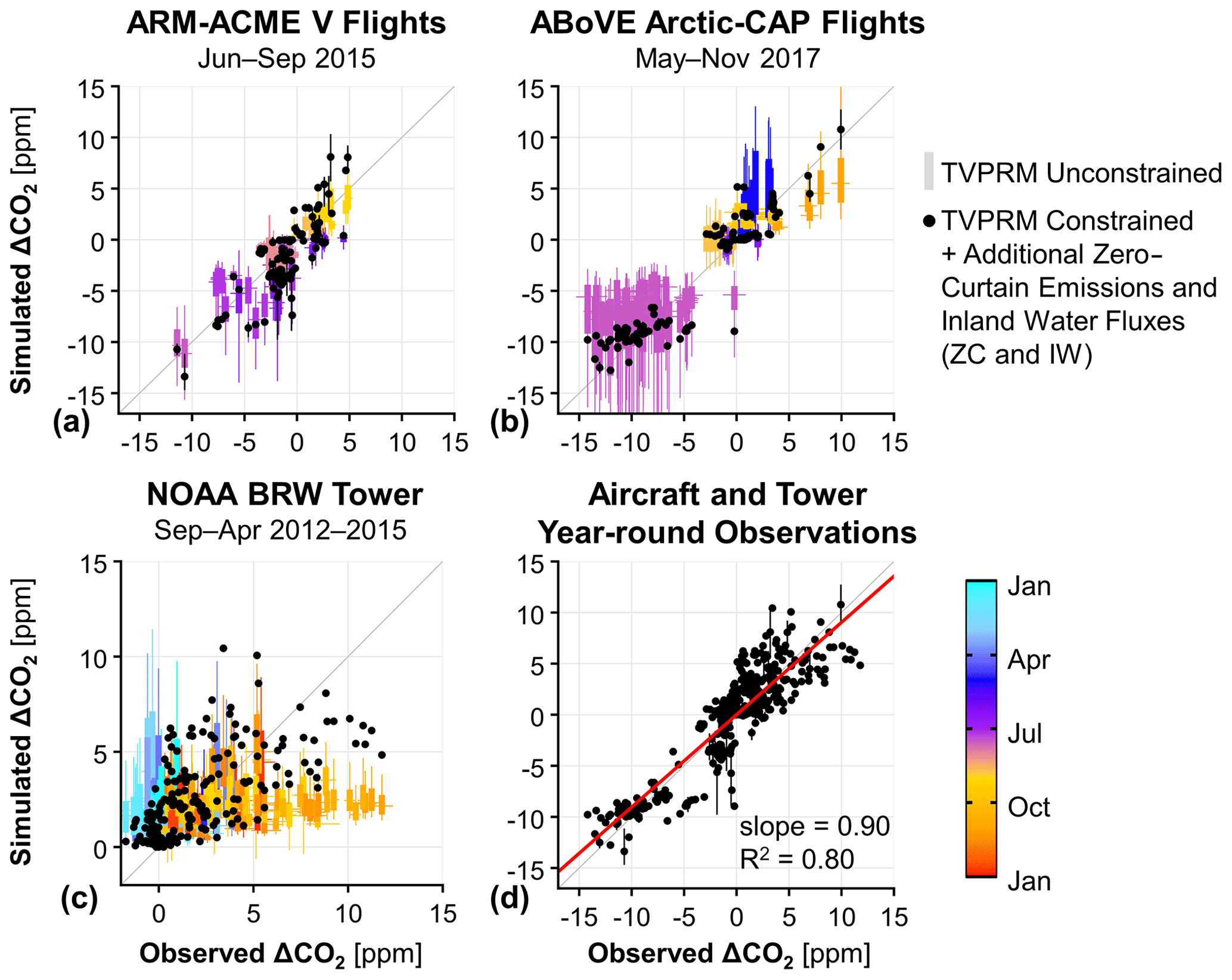
Figure 2 Aircraft and tower CO₂ concentration measurements constrain year-round simulated CO₂ fluxes on the Alaska North Slope. (a–c) Comparison of observed and simulated ΔCO₂ during the ARM-ACME V flight campaign (a), during the ABoVE Arctic-CAP flight campaign (b), and at the NOAA BRW tower (c) for air over the Alaska North Slope. Horizontal lines indicate the range of uncertainty in the NOAA BRW tower ocean-sector background calculation. Vertical boxes colored by month of the year represent 50 % and whiskers represent 95 % of the ΔCO₂ values from all members of the unconstrained TVPRM ensemble (see Sect. 2.4) from all binned points. Black points show values from the constrained TVPRM member with additional zero-curtain (ZC) emissions and inland water (IW) fluxes (see Sect. 3.4). For panels (a) and (b), observed values are vertically binned medians, and vertical lines contain the middle 95 % of ΔCO₂ values from all binned points for the constrained TVPRM member + ZC and IW. (d) Combined comparison of observed and simulated ΔCO₂ for all aircraft and tower points using the constrained TVPRM member + ZC and IW. The linear best fit (red line), the slope determined by ordinary least squares, and the coefficient of determination (R²) of all points (n=455) are shown. The 1:1 is line shown in dark gray.

These comparisons enable us to constrain the regional net CO₂ flux on the Alaska North Slope. First, we identify the year-round empirically driven net CO₂ fluxes from the TVPRM ensemble (TVPRM Unconstrained) which are most consistent with the CO₂ concentration observations from the two aircraft campaigns and at the tower (TVPRM Constrained) (Sect. 3.1 and 3.2). Then, noting the large range of potential cold-season CO₂ fluxes, we compare our constrained TVPRM member with CO₂ fluxes from previous studies (Sect. 3.3). Finally, we suggest and quantify sources of the missing CO₂ flux observed during the early cold season (defined here as September–December) and incorporate those fluxes into our net CO₂ budget (TVPRM Constrained + Additional Zero-Curtain Emissions and Inland Water Fluxes) (Sect. 3.4). This analysis provides a unique regional net CO₂ flux quantification for the North Slope that is verified using atmospheric observations and can also be explained from an ecological and physical perspective.

3 Results

3.1 Evaluation of the unconstrained empirical net CO₂ flux model ensemble

3.1.1 Using aircraft-observed CO₂ enhancements

The observed ΔCO₂ during the ARM-ACME V (June–September 2015) and ABoVE Arctic-CAP (May–November 2017) airborne campaigns show a strong seasonal uptake pattern throughout the growing season (Fig. 2a, b). The frequent flights during ARM-ACME V (multiple flights per week) observe the transition from early to peak growing season uptake (observed ΔCO₂ = −11 ppm) and on into cold-season respiration, which results in net CO₂ source conditions in September (+5 ppm). While less frequent, the ABoVE Arctic-CAP flights begin at the end of the cold season, extend later into following cold season, and cover a larger area of the North Slope. Peak growing season uptake observed by the ABoVE Arctic-CAP flights (−14 ppm) is slightly stronger than for during ARM-ACME V, and the ABoVE Arctic-CAP flights observe a strong CO₂ source throughout the North Slope (+10 ppm) by November. The difference in observed ΔCO₂ during peak growing season uptake between 2015 and 2017 is likely similar to the uncertainty in the respective values and could be due to differences in areas of the North Slope sampled between years.

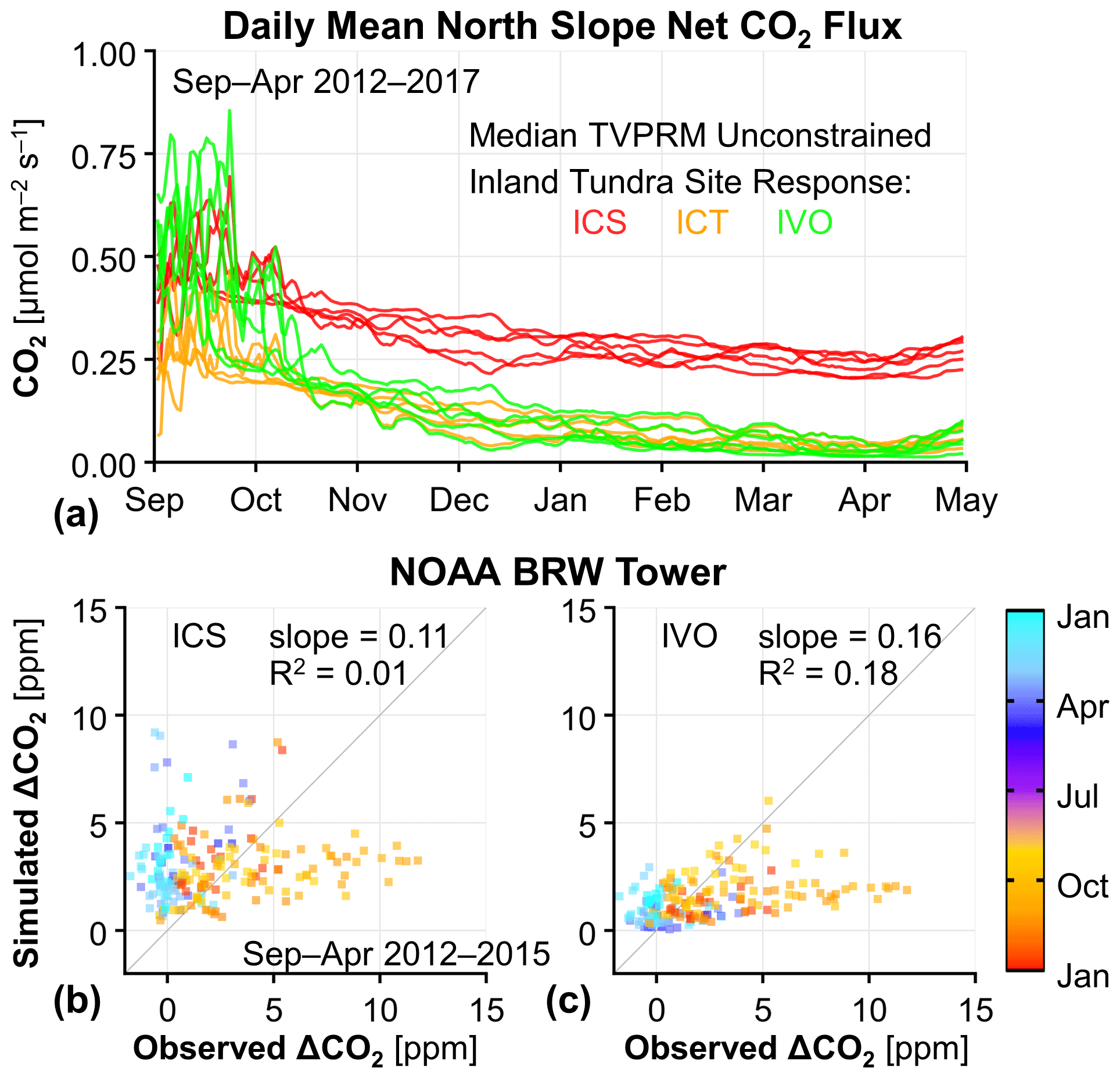
Figure 3 Cold-season CO₂ emissions for the inland tundra site parameterizations and comparison to tower observations. (a) Time series of simulated daily mean Alaska North Slope net CO₂ flux for the median of all unconstrained TVPRM ensemble members using each of the three inland tundra site parameterizations: ICS (red), ICT (orange), and IVO (green). Yearly colored lines shown for September–April beginning in September 2012 and ending in April 2017. The same is shown for all eight eddy flux sites in Fig. S9. (b, c) Comparison of observed and simulated ΔCO₂ at the NOAA BRW tower for air over the North Slope using the median of all unconstrained TVPRM ensemble members for the inland tundra site parameterizations at ICS (b) and IVO (c). All points are colored by day of year. The slope determined by ordinary least squares and the coefficient of determination (R²) of all points (n=191) are shown. The 1:1 line is also shown in dark gray.

The magnitude and timing of the observed net CO₂ uptake throughout the growing season is generally well represented by the empirical net CO₂ flux model ensemble (TVPRM Unconstrained; Figs. 2a, b, and S6). The median coefficients of determination (R²) and ordinary least squares slopes between the observed and simulated ΔCO₂ for this time are 0.54 and 0.41 for ARM-ACME V and 0.82 and 0.72 for ABoVE Arctic-CAP, respectively. Only for the July observations during the ABoVE Arctic-CAP campaign do many members of the CO₂ flux trend toward an underestimate of net CO₂ uptake, with all points showing a much larger range of simulated values compared to ARM-ACME V. The net CO₂ release tends to be overestimated by the TVPRM ensemble during the ABoVE Arctic-CAP seasonal transitions in May and September, but the observed R_soil is consistently underestimated during November.

Given the large range of unconstrained representations of the regional CO₂ flux, the accuracy in simulating the aircraft-observed ΔCO₂ varies between TVPRM ensemble members. For example, members using the RasterCAVM vegetation map, which places less coastal tundra area cover in the south (Fig. S5), produce a smaller mean July net CO₂ uptake flux (by ∼ 1 $\mathrm{\mu }\mathrm{mol}{\mathrm{m}}^{-\mathrm{2}}{\mathrm{s}}^{-\mathrm{1}}$, Fig. S7a) throughout the southern North Slope than members using other vegetation maps (CAVM and ABoVE LC), and this placement consistently underestimates the net ΔCO₂ uptake during the growing season by 5–10 ppm compared with the aircraft observations (Fig. S8). Also, members driven by SIF products that integrate additional remote sensing and/or meteorological data (GOSIF and CSIF) better reflect the timing and magnitude of the peak season carbon uptake in tundra ecosystems than members produced by interpolated SIF retrievals (GOME-2 SIF product), which underestimate the observed CO₂ uptake during July (Fig. S8).

Using these comparisons, we identify less-representative ensemble members that generally underestimate the observed ΔCO₂ uptake during the growing season (RasterCAVM vegetation map and GOME-2 SIF product members). Removing these members from the TVPRM ensemble improves the collective performance of the remaining members during the growing season (Fig. S6), brings the median slope of agreement closer to 1 for both campaigns (improves from 0.53 to 0.64 and from 0.71 to 0.94 for ARM-ACME V and ABoVE Arctic-CAP, respectively), and reduces the median NMB (−0.34 to −0.03) and median RMSE (3.12 to 2.73) for ABoVE Arctic-CAP.

3.1.2 Using tower-observed CO₂ enhancements

As seen with the September–November aircraft data, the observed ΔCO₂ at the NOAA BRW tower (Fig. 2c) indicate that the CO₂ source to the atmosphere increases substantially from September to peak in October and November (+12 ppm) before decreasing to near zero throughout the late cold season (January–April).

Most of the TVPRM ensemble members substantially underestimate the observed ΔCO₂ in the early cold season (September–December) as the soils freeze, and some simulations produce too much CO₂ in the late cold season when the soils are frozen (Fig. 2c). The cold-season CO₂ flux differs greatest in magnitude and spatial extent between the ensemble members parameterized for the ICS and ICT inland tundra sites (Figs. 3a, S9, S10), with a net CO₂ flux difference of ∼ 0.2 $\mathrm{\mu }\mathrm{mol}{\mathrm{m}}^{-\mathrm{2}}{\mathrm{s}}^{-\mathrm{1}}$ throughout the region (Fig. S7b).

While the magnitude of CO₂ flux from ICS members better matches the observed ΔCO₂ in the early cold season than that from other sites (Figs. 3b, c, and S11), the response to T_s at ICS shows only a modest decrease in CO₂ flux between the early and late cold season (32 % decrease between October and March; Fig. 3a), resulting in an overestimate of the regional ΔCO₂ in the late cold season. The CO₂ flux response to T_s for ICT members is similar to that for ICS but lower in magnitude, and the simulated ΔCO₂ from members of neither site performs well against the observations in both the early and late cold season. Therefore, ICS and ICT inland tundra responses to T_s are not representative of the regional ΔCO₂ observed at the NOAA BRW tower throughout the entire cold season, and we remove those members from our TVPRM ensemble.

The observed net CO₂ fluxes at the IVO inland tundra and CMDL coastal tundra sites both show prolonged zero-curtain emissions (Fig. S1) and respond strongly to T_s in the early cold season (Fig. S9). The stronger response of CO₂ fluxes to T_s from the early to late cold season at IVO (70 % decrease by January; Fig. 3a) compared with at the Imnavait Creek sites produces TVPRM members that better represent the large regional decrease in ΔCO₂ observed on the North Slope (Fig. 3c). While all coastal tundra sites respond similarly to T_s during the cold season, we determine that the CO₂ flux magnitude at CMDL is most consistent with the regional observations (Fig. S11). T_s values from ERA5 remain warmer throughout the late cold season compared with those from NARR, which causes simulations using ERA5 T_s to overestimate CO₂ release during that time (Fig. S11). Unlike during the growing season, cold-season CO₂ fluxes are not sensitive to the vegetation distribution nor the SIF products.

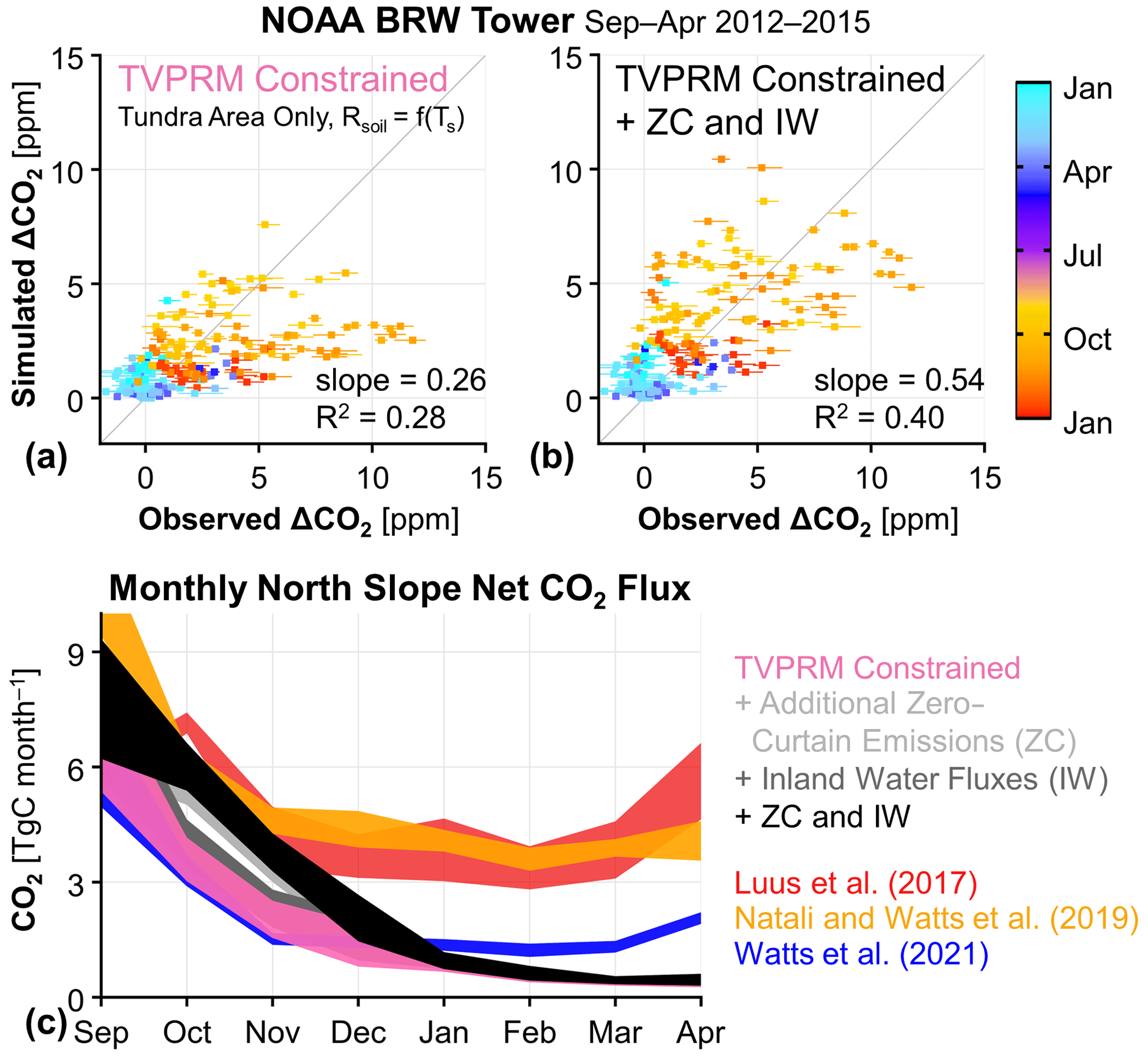
Figure 4 Tall-tower atmospheric observations of the Alaska North Slope support early-cold-season emissions not driven by soil temperature (T_s) and present no evidence of elevated late-cold-season emissions. (a, b) Comparison of hourly cold-season (September–April) observed and simulated ΔCO₂ at the NOAA BRW tower for the constrained TVPRM member, where soil respiration (R_soil) is determined only by T_s (a) and for the constrained TVPRM member + additional zero-curtain (ZC) emissions and inland water (IW) fluxes (b). Horizontal segments indicate the range of uncertainty in the NOAA BRW tower ocean-sector background calculation. The slope determined by ordinary least squares and the coefficient of determination (R²) of all points (n=191) are shown. The 1:1 line is also shown in dark gray. (c) Monthly cold-season total Alaska North Slope net CO₂ fluxes for various CO₂ flux models. TVPRM-based simulations and Natali and Watts et al. (2019) show values for 2012–2017, Luus et al. (2017) show 2012–2014, and Watts et al. (2021) show September 2016–April 2017. Ribbons represent the range of all years, where applicable. The area of the North Slope domain used to calculate regional totals is 3.537×10⁵ km².

Finally, we identify the TVPRM member that best matches the observed ΔCO₂: parameterized by IVO inland tundra and CMDL coastal tundra site responses, distributed by the ABoVE LC vegetation map, and driven by NARR reanalysis and the CSIF SIF product (referred to here as TVPRM Constrained; Figs. S6, S12). This constrained simulation estimates a mean regional CO₂ flux of 0.05 $\mathrm{\mu }\mathrm{mol}{\mathrm{m}}^{-\mathrm{2}}{\mathrm{s}}^{-\mathrm{1}}$ for the late cold season in 2012–2015 and reproduces the observed ΔCO₂ during this time well (Fig. 4a). The late-cold-season NMB and RMSE against the observations at the NOAA BRW tower are reduced from 4.91 to 2.04 and from 1.94 to 1.30, respectively, for the constrained simulation compared with the median of the entire TVPRM ensemble (Fig. S12). However, the early-cold-season CO₂ emissions, with a mean regional CO₂ flux of 0.25 $\mathrm{\mu }\mathrm{mol}{\mathrm{m}}^{-\mathrm{2}}{\mathrm{s}}^{-\mathrm{1}}$ for September–December (Fig. S13a), are still underestimated, with the simulated ΔCO₂ lower than the observed ΔCO₂ by ∼5 ppm (Fig. 4a).

3.2 Alternative T_s products and R_soil parameterizations

To test the impact of reanalysis T_s on the early-cold-season CO₂ fluxes, we implement T_s values that are more specifically developed to represent Alaska tundra permafrost soils during freeze–thaw processes than the reanalysis products driving our constrained TVPRM member. A single layer of T_s at 8 cm depth from RS-PM (Fig. S14a) captures the magnitude and temporal behavior of the observed early-cold-season CO₂ fluxes slightly better than the constrained member (Figs. 4a, S12), which uses NARR reanalysis T_s and does not incorporate permafrost-model-derived T_s. The RS-PM T_s extends CO₂ emission fluxes further into the cold season by up to a month, which is consistent with a better representation of the zero-curtain period; however, emissions remain higher throughout the late cold season than our atmospheric-observation-constrained CO₂ fluxes (Fig. S15). We also test the implementation of a multilayer fit driven by soil column temperature from RS-PM, but neither of these instances of remote-sensing-informed T_s substantially improve the agreement of the ΔCO₂ at the NOAA BRW tower during the early cold season. Attempts to use alternative R_soil formulations based on T_s, including Q₁₀ relationships, also fail to reproduce the observed elevated CO₂ fluxes during the cold season.

3.3 Evaluation of other CO₂ flux models during the cold season

More early-cold-season (September–December) CO₂ flux into the atmosphere is observed at the NOAA BRW tower than is emitted by our constrained empirical simulation member, and these observations also indicate low late-cold-season (January–April) CO₂ emissions. We compare our constrained CO₂ fluxes to several other representations of gridded CO₂ flux on the North Slope (Table S3) and find that difficulty in simulating the magnitude and timing of the observed ΔCO₂ throughout the cold season is not unique to the constrained fluxes from our study.

The net CO₂ fluxes from Luus et al. (2017) are similar to the constrained TVPRM member during the growing season (Fig. S16) but release more than 3 times as much CO₂ into the atmosphere throughout the late cold season (Fig. 4c). This large late-cold-season CO₂ flux leads to a large overestimate compared with the observed ΔCO₂ (Fig. S14b). The optimization employed by Commane et al. (2017) increases the September–October CO₂ flux to a range that matches our observations at the NOAA BRW tower. However, Commane et al. (2017) did not optimize the cold-season fluxes from November to March, instead reverting to Luus et al. (2017) fluxes during this time, and thus produced late-cold-season fluxes that are too large. Overall, Commane et al. (2017) projected a regional total cold-season CO₂ source of 37–40 Tg C for 2012–2014, which is more than twice as high as our constrained TVPRM member CO₂ flux (15–18 Tg C) for those years.

Carbon dioxide fluxes from work by Natali and Watts et al. (2019), a cold-season model developed for the global high-latitude permafrost region, are similar to our constrained TVPRM member in September, but the fluxes remain high throughout the cold season (Fig. 4c), similarly to Luus et al. (2017), for a range of total cold-season CO₂ flux of 40–43 Tg C for 2012–2017. This sustained CO₂ release also leads to an overestimation in the ΔCO₂ in the late cold season for this region (Fig. S14c). Tao et al. (2021) also show that the cold-season CO₂ fluxes of Natali and Watts et al. (2019) are high compared with their model. More recent work by Watts et al. (2021), using observations from new Soil Respiration Station monitoring sites in Alaska, produces cold-season CO₂ fluxes more similar to our constrained CO₂ fluxes, with an underestimate in the simulated ΔCO₂ during the early cold season (Fig. S14d), for a total cold-season CO₂ flux of 18 Tg C for September 2016 to April 2017.

3.4 Sources of missing CO₂ fluxes

None of the flux products discussed above, including our TVPRM ensemble, account for any potential CO₂ fluxes during the zero-curtain period that are not driven by T_s or are from areas on the terrestrial–aquatic interface. To account for these processes, we first add an additional CO₂ flux with zero-curtain timing to our constrained CO₂ flux (TVPRM) member from both inland and coastal tundra areas that consists of 0.25 $\mathrm{\mu }\mathrm{mol}{\mathrm{m}}^{-\mathrm{2}}{\mathrm{s}}^{-\mathrm{1}}$ for October with a reduction to 0 by the end of December. This peak additional CO₂ flux is within the daily variability in the observed CO₂ flux at the IVO and CMDL eddy flux sites during the zero-curtain period (Fig. S9), and the reduction into December is consistent with these observations. The additional zero-curtain flux improves the ability of the model to reproduce the observed ΔCO₂ at the NOAA BRW tower (slope = 0.46, R² = 0.41). We also apply the coastal tundra site ecosystem parameterization used in our constrained TVPRM member to all areas of inland water on the North Slope, which account for 4 % of the domain according to the ABoVE LC map (Fig. S5) and were previously set to zero CO₂ flux. Representing these aquatic areas with biogenic CO₂ fluxes consistent with coastal tundra ecosystems is one simple way to bridge the terrestrial–aquatic gap in tundra ecosystem models, where portions of aquatic systems on the land–water gradient (i.e., the edges) may be more likely to respond to the environment as coastal tundra than with the zero-flux assumed by water area. The ice phenology for areas of inland water producing CO₂ flux is then considered to be similar to that of the freeze–thaw timing in coastal tundra soils. Adding these coastal tundra fluxes to inland water areas also improves the performance of our model (slope = 0.32 and R² = 0.29 against NOAA BRW tower observations). The magnitude of additional zero-curtain flux suggested here and the portion of inland water represented with coastal tundra site parameterizations produce the best statistical comparison for a range of choices tested (Fig. S17).

Together, adding these zero-curtain (ZC) and inland water (IW) CO₂ fluxes to our constrained simulation (referred to as TVPRM Constrained + ZC and IW) increases the mean regional CO₂ flux in the early cold season by 70 % (0.18 $\mathrm{\mu }\mathrm{mol}{\mathrm{m}}^{-\mathrm{2}}{\mathrm{s}}^{-\mathrm{1}}$; Fig. S13b) and results in a large improvement to our comparison of ΔCO₂ at the NOAA BRW tower (slope =0.54, R²=0.40; Figs. 4b, S12) and across the region using airborne data, especially during the November ABoVE Arctic-CAP flights (Figs. 2, S6). The year-round comparison using all available aircraft and tower observations shows that these net CO₂ fluxes are now representative of the region (slope =0.90, R²=0.80; Fig. 2d). As a result, the North Slope regional total cold-season CO₂ flux increases by 6 Tg C (∼38 %) to 20–24 Tg C for 2012–2017 compared with the constrained empirical CO₂ flux model member.

3.5 Alaska North Slope annual net CO₂ flux

The median Alaska North Slope annual net CO₂ flux from the TVPRM ensemble (−5 Tg C yr⁻¹) for 2012–2017 is consistent with the previous multi-model comparison (Fisher et al., 2014), but we find a much smaller range of regional CO₂ flux values (26 to −29 Tg C yr⁻¹ for 95 % of TVPRM members; Fig. S18). The largest contribution to this ensemble range comes from the difference in parameterizations determined for the ICS and ICT inland tundra sites, with TVPRM members using ICS trending toward a net CO₂ source, while ICT trends toward net CO₂ uptake. The distribution of inland and coastal tundra throughout the region represented by the vegetation maps also has a noticeable impact on the sign of the net CO₂ flux, with members using the RasterCAVM more likely to release net CO₂ into the atmosphere than members using the other maps. There is also little interannual variability in the unconstrained TVPRM ensemble, with only 2014 moving toward a net CO₂ source, consistent with Tao et al. (2021) for these years.

Figure 5 Annual and seasonal Alaska North Slope net CO₂ flux constrained by aircraft and tower observations. (a) Annual, (b) late-cold-season (January–April), (c) growing-season (May–August), and (d) early-cold-season (September–December) total Alaska North Slope net CO₂ fluxes for various CO₂ flux models for 2012–2017, as in Fig. 4. Purple squares indicate the middle 95 % of all TVPRM ensemble members.

Our best quantification of the annual net CO₂ flux for the North Slope informed by atmospheric observations, TVPRM Constrained + ZC and IW, indicates that the region is a small net sink for 2013 (−5 Tg C yr⁻¹) and 2015 (−6 Tg C yr⁻¹) and a small net source for 2012 (+6 Tg C yr⁻¹), 2014 (+6 Tg C yr⁻¹), 2016 (+2 Tg C yr⁻¹), and 2017 (+2 Tg C yr⁻¹) (Fig. 5a). We estimate a 10 % uncertainty in the net annual CO₂ flux based on the slope from our final comparison with the year-round observations (Fig. 2d). The year-round net CO₂ fluxes from Luus et al. (2017) (driven with NARR meteorology, monthly GOME-2 SIF, and the CAVM vegetation map) indicate the North Slope to be a strong annual net CO₂ source for 2012–2014 (+9 to +15 Tg C yr⁻¹; Fig. S18) and are inconsistent with our results. Our results are more consistent with Tao et al. (2021), but we find a smaller range in the magnitude of net CO₂ flux over the same years and more years trending toward a net CO₂ source.

We find that the regional net growing season CO₂ uptake and the cold-season emissions on the North Slope are comparable in magnitude, so the net balance could depend on small perturbations in either flux. However, the regional cold-season CO₂ emissions for these years were relatively similar from year to year: 18–21 Tg C for the early cold season (Fig. 5d), diminishing to only 2–3 Tg C for the late cold season (Fig. 5b). Therefore, the interannual variability in the regional carbon balance is largely driven by fluctuating net growing season CO₂ fluxes during these years: greater net growing season uptake in 2013 and 2015 than in 2012, 2014, 2016, and 2017 (Fig. 5c).

4 Discussion

4.1 Tundra ecosystem growing season net CO₂ fluxes

The good performance of the TVPRM ensemble against the atmospheric observations during the growing season indicates that the tundra ecosystems of the Alaska North Slope respond to light and heat, as quantified by PAR, T_s, and T_a, and that the net CO₂ flux is largely controlled by the simple R_soil, R_plant, and GPP relationships in the empirical model over this time.

The growing season of each year determines the sign of the regional annual net CO₂ flux during our study period, with 2013 and 2015 being strong net sinks and 2014 being the strongest net source. The relative magnitude of each component of the net CO₂ flux during the growing season (i.e., R_soil, R_plant, and GPP) varies from year to year (Table S7) and helps explain the interannual variability in the net source or sink status of the North Slope. The growing season in 2015 was very warm, dry, and sunny in Alaska and resulted in extreme biomass burning activity outside of the North Slope (Table S1). High regional mean T_a and PAR (Table S8) and low accumulated precipitation (Table S9) in NARR confirm this was the case for North Slope as well, with high T_a and PAR contributing to a very high GPP. The growing season SIF signal from the CSIF product, which determines the seasonal cycle and relative magnitude of photosynthetic activity, is also large in 2015 (Table S8), further enhancing GPP. This year and others with a larger GPP component of NEE correspond to growing seasons with stronger SIF signals, which is an indicator of increased productivity and consistent with previous studies (e.g., Magney et al., 2019; Sun et al., 2017). While fairly high T_a and T_s in 2015 also result in high R_soil and R_plant, respectively, this elevated respiration is not enough to offset the very high GPP and results in a large net CO₂ sink. In contrast, the summer of 2014 was cool, wet, and cloudy, and the North Slope experienced a very low T_a, PAR, and SIF signal, producing very low GPP. Lower-than-normal T_a also results in very low R_plant, but (as for 2015) this is not enough to offset the extremely low uptake, resulting in a large net CO₂ source for 2014. In 2013, the other growing season with a strong net CO₂ sink, moderately high GPP combines with moderately low R_plant and very low R_soil. Extremely low T_s causes this very low R_soil, which, relative to moderate T_a and PAR, is likely a result of an above-average lingering snowpack into May (Table S9). This lingering snowpack is perhaps surprising given that the mean snowpack for the proceeding cold season was not particularly deep. The important impact that snow cover and the timing of snowmelt has on T_s and carbon response in tundra ecosystems has recently been emphasized (e.g., Kim et al., 2021) and is also supported by our work, which shows that the prevalence of snow in the spring may determine the sign of the regional net CO₂ for an entire year.

The regional net CO₂ flux is highly sensitive, however, to the distribution of tundra vegetation types (upland vs. coastal) throughout the North Slope during the growing season. Coastal tundra takes up more CO₂ for a given unit PAR compared with inland tundra, based on the relationships between observed site-level net CO₂ flux and PAR in this study (TVPRM parameters; Fig. S1), which could be evidence of an adaptation to lower light levels. This difference is consistent with Luus et al. (2017), who calculated greater uptake at “wetland” sites like Atqasuk and Barrow than at “graminoid tundra” sites like Ivotuk and Imnavait when all driver inputs are constant, and with Mbufong et al. (2014), who also found that peak growing season net uptake for constant light is greater at Barrow than at Ivotuk. The stronger CO₂ uptake response of coastal tundra to light is important to consider due to the fact that the vegetation distributions assessed here, with more coastal tundra to the south (CAVM, Walker et al., 2005; ABoVE LC, Wang et al., 2020), better agree with the atmospheric observations. When considering the ability of coastal tundra to take up CO₂ when moved toward the south, Patankar et al. (2013) saw that tundra plants exposed to additional intense light did not respond with additional uptake. Therefore, while the ecosystem response of the southern North Slope is more consistent with coastal ecosystems, it seems possible that these areas are misclassified in either our simplified two-tundra-type scheme or in the vegetation maps themselves. The large variability in net CO₂ flux calculated using the different maps supports the importance of accurate ecosystem type locations in upscaling eddy flux measurements and highlights the need for improved vegetation mapping and classification schemes in the Arctic ecology research community.

4.2 Regional-scale cold-season CO₂ emissions

Observations across scales, at the in situ eddy flux towers, the NOAA BRW tower, and from aircraft, consistently show signs of large early-cold-season CO₂ emissions from ecosystems on the Alaska North Slope. However, there is no evidence of widespread elevated emissions in this region during the late cold season, contrary to other studies (Commane et al., 2017; Natali and Watts et al., 2019). The TVPRM ensemble parameterizations using terrestrial eddy flux sites and the fluxes from other terrestrial CO₂ models cannot reproduce both the observed magnitude and across-season timing of these cold-season CO₂ emissions.

The largest differences in the net CO₂ flux between TVPRM ensemble members result from the contrasting site conditions driving the ICS and ICT R_soil parameterizations during the cold season. When taken separately by cold-season segment, ICS members perform quite well against observations at the NOAA BRW tower for the early cold season and ICT members perform well for the late cold season. The contrasting performance between site parameterizations is due to the topographic and hydrologic conditions, which are quite heterogeneous over a short distance and influence the plant communities and carbon storage, at each site. The ecosystems sampled by the ICS tower are seasonally inundated and retain a deep layer of organic soil that can be respired in greater amounts longer into the early cold season, whereas the well-drained hillslope at ICT does not allow for the accumulation of organic matter in the same way (Euskirchen et al., 2017; Larson et al., 2021). While varying topography and soil inundation throughout the North Slope means that each of these site relationships is likely to be representative of many other locations in the region with similar conditions, the early- to late-cold-season reduction in CO₂ fluxes at these sites is not consistent with the observed regional atmospheric trend, and we remove the members parameterized by them from the ensemble. Individual eddy flux site parameterizations may reproduce regional CO₂ fluxes for a given season, but it is important to consider their response to drivers across multiple seasons when scaling from the site-level to regional domains.

The observed cold-season CO₂ flux pattern on the North Slope may be unique to tundra ecosystems of this region. For example, the CO₂ fluxes from Natali and Watts et al. (2019) and Watts et al. (2021) both incorporate measurements from the North Slope. However, Natali and Watts et al. (2019) used boosted regression trees trained on belowground respiration measurements from across the pan-Arctic tundra and boreal zones, which may not be representative of our study region. The fluxes from Watts et al. (2021) are based on respiration measurements from throughout only Alaska and northwest Canada and conform better to local conditions. The evaluation of these CO₂ fluxes against atmospheric CO₂ measurements also produces results that are more consistent with our TVPRM ensemble determined by North Slope eddy flux tower measurements.

We find that the atmospheric observations are best matched by biogenic CO₂ fluxes that include an additional CO₂ source from tundra ecosystems during the zero-curtain period that are independent of T_s variability and year-round net CO₂ fluxes from areas of inland water. The additional zero-curtain flux represents large-scale emission events that are not directly timed to microbial activity and root respiration controlled by T_s but that could be related to the delayed physical release of previously produced CO₂ from soil through the snowpack as the soil layers remain unfrozen (Bowling and Massman, 2011). The Alaska North Slope also has many waterbodies distributed throughout the coastal tundra region, and the extent to which carbon cycles between small, shallow ponds and their surrounding terrestrial components is unclear (Magnússon et al., 2020). The biogenic CO₂ fluxes in these areas are likely driven by ecosystem-scale CO₂ fluxes from both coastal tundra and small ponds (Holgerson and Raymond, 2016; Tan et al., 2017), and their impact on the regional net CO₂ flux, via both emissions and uptake, may be significant (Elder et al., 2018; Beckebanze et al., 2022). Only by adding fluxes that match observed zero-curtain CO₂ emission pulses and by approximating net CO₂ fluxes in aquatic areas can we reproduce the observed ΔCO₂ magnitude in both the early and late cold season. The resulting seasonal change between the early and late cold season is consistent with the extended duration of the observed regional-scale zero curtain. The simplistic approximations suggested here are not inconsistent with the existing uncertainties in tundra CO₂ flux modeling and demonstrate the importance of considering these additional CO₂ fluxes and their mechanisms for future study.

4.3 Future state of net CO₂ flux on the Alaska North Slope

As the Arctic warms rapidly, the competition between the growing and cold-season Arctic CO₂ fluxes will determine the net biogenic CO₂ flux into the atmosphere. Warming T_a warms soils, thaws permafrost, increases the active-layer thickness, and has extended the duration of the zero curtain from weeks to over 100 d (Romanovsky and Osterkamp, 2000; Schuur et al., 2015; Zona et al., 2016), all of which increase cold-season CO₂ emissions. The warming may also increase net growing season uptake, but the severe light limitation at high northern latitudes limits the extent of the growing season, especially on the North Slope (Zhang et al., 2020). The future of CO₂ fluxes from inland waters and wetlands in the Arctic is uncertain, but some studies suggest CO₂ emissions from lakes may increase (Bayer et al., 2019). The culmination of these effects will likely push the North Slope into being a consistent net source in the future. However, observations at the NOAA BRW tower during our study period do not show elevated late-cold-season CO₂ emissions; therefore, the North Slope was not a consistent net source through 2017. Accordingly, care must be taken to accurately represent CO₂ fluxes from Arctic ecosystems during both the early and late cold season when calculating the annual net CO₂ budget. TVPRM could be used with projections of meteorology and SIF to calculate the future net CO₂ balance for this region, but we caution against overuse of the model using current parameters, as the flux–driver relationships in the rapidly warming Arctic ecosystems are changing so quickly that we would not assume accuracy into the future. While we can constrain the annual net CO₂ budget with existing data, the Arctic is rapidly changing and needs constant monitoring. The following recommendations would provide more detailed spatial and seasonal constraints and up-to-date information on the processes driving CO₂ fluxes across the region.

4.3.1 Future observation efforts

Our results motivate the need for a more extensive network of CO₂ eddy flux towers operating year-round, alongside sensors for soil moisture and T_s profiles throughout the active layer to better understand the mechanisms driving year-round and especially early-cold-season CO₂ fluxes. Noting that automated or semiautomated monitoring systems for aquatic environments currently do not exist for the North Slope or other high-latitude regions, this sensor network should be distributed throughout poorly sampled ecosystem types, particularly along wetness gradients that span mixed terrestrial–aquatic environments. The results of this study also support the need for additional continuous CO₂ concentration measurements at tall towers across the North Slope (including away from the coast) to increase coverage of observed ΔCO₂ during all seasons and to better constrain the regional background. Airborne measurements of both CO₂ concentrations and CO₂ fluxes remain valuable to sample areas less accessible via ground-based measurements, but a large-scale flight campaign in the region has not occurred since 2017. Any additional flights should be targeted as early before, and as late after, the growing season as possible. Satellites that rely on reflected sunlight to detect CO₂ have increasingly been used to constrain CO₂ budgets in the northern latitudes (e.g., Byrne et al., 2022), but data are very limited in the cold season, especially in far northern regions like the North Slope.

4.3.2 Future modeling efforts

The large initial range of potential regional net CO₂ flux values that we found for the Alaska North Slope indicates a large sensitivity to the choices and assumptions made when scaling eddy flux observations from the site to the regional scale. The most important of these choices are the representation of the upland tundra, particularly for the response of R_soil to T_s during the cold season, and the distribution of vegetation types throughout the domain. Future tundra CO₂ modeling efforts should focus on using site-level data that are the most consistent with regional-scale fluxes, rather than incorporating data from all available sites. Consistency and accuracy in classification schemes used in vegetation maps must also be addressed. As we have shown with the atmospheric observations, not all model scenarios have equal likelihood to be true, and the mean of the model ensemble is not necessarily the most likely or most consistent with the atmosphere. Using these atmospheric observations is uncertain, however, due to potential errors in the transport modeling, which are difficult to quantify. Atmospheric modeling of remote areas such as the Alaska North Slope requires further evaluation and improvement. Moreover, increasing the model temporal resolution should be considered, as the importance of the zero-curtain and snow cover to the net CO₂ flux of tundra ecosystems is recognized, both of which vary on the order of days and weeks, rather than months.

5 Conclusions

Observed atmospheric concentrations from aircraft and towers are a powerful tool that provide a regional constraint on the many combinations of possible CO₂ flux parameterizations and distributions of tundra ecosystems on the North Slope of Alaska. We find that the annual regional net CO₂ flux on the North Slope in not a consistent net source nor sink but instead varies between −6 and +6 Tg C yr⁻¹ for 2012–2017. We can also identify ecosystem relationships and driver combinations that best represent both local CO₂ flux patterns and regional atmospheric CO₂ enhancements. The simulated regional net CO₂ flux is highly sensitive to the assumptions made while scaling up eddy flux observations, especially the ecosystem response to T_s of tundra during the cold season and the spatial distribution of tundra types across the North Slope. Additionally, scaling methods that average observations from multiple eddy covariance flux sites should consider which sites are most representative of the regional impact of the biosphere on the atmosphere using integrative top-down observations.

This work shows that year-round measurements of atmospheric CO₂ concentrations and fluxes across heterogeneous terrestrial and aquatic ecosystems are needed to represent the drivers of CO₂ fluxes from Arctic regions. Arctic ecosystems have the potential to accelerate warming if vast stores of carbon are released or to buffer warming if increasing carbon uptake from vegetation occurs. All components of Arctic tundra ecosystems must be fully incorporated into Earth system models to improve projections of future climate warming and associated carbon cycle feedbacks.