The representation of alkalinity and the carbonate pump from CMIP5 to CMIP6 Earth system models and implications for the carbon cycle

Ocean alkalinity is critical to the uptake of atmospheric carbon in surface waters and provides buffering capacity towards the associated acidification. However, unlike dissolved inorganic carbon (DIC), alkalinity is not directly impacted by anthropogenic carbon emissions. Within the context of projections of future ocean carbon uptake and potential ecosystem impacts, especially through Coupled Model Intercomparison Projects (CMIPs), the representation of alkalinity and the main driver of its distribution in the ocean interior, the calcium carbonate cycle, have often been overlooked. Here we track the changes from CMIP5 to CMIP6 with respect to the Earth system model (ESM) representation of alkalinity and the carbonate pump which depletes the surface ocean in alkalinity through biological production of calcium carbonate and releases it at depth through export and dissolution. We report an improvement in the representation of alkalinity in CMIP6 ESMs relative to those in CMIP5, with CMIP6 ESMs simulating lower surface alkalinity concentrations, an increased meridional surface gradient and an enhanced global vertical gradient. This improvement can be explained in part by an increase in calcium carbonate (CaCO₃) production for some ESMs, which redistributes alkalinity at the surface and strengthens its vertical gradient in the water column. We were able to constrain a particulate inorganic carbon (PIC) export estimate of 44–55 Tmol yr⁻¹ at 100 m for the ESMs to match the observed vertical gradient of alkalinity. Reviewing the representation of the CaCO₃ cycle across CMIP5/6, we find a substantial range of parameterizations. While all biogeochemical models currently represent pelagic calcification, they do so implicitly, and they do not represent benthic calcification. In addition, most models simulate marine calcite but not aragonite. In CMIP6, certain model groups have increased the complexity of simulated CaCO₃ production, sinking, dissolution and sedimentation. However, this is insufficient to explain the overall improvement in the alkalinity representation, which is therefore likely a result of marine biogeochemistry model tuning or ad hoc parameterizations. Although modellers aim to balance the global alkalinity budget in ESMs in order to limit drift in ocean carbon uptake under pre-industrial conditions, varying assumptions related to the closure of the budget and/or the alkalinity initialization procedure have the potential to influence projections of future carbon uptake. For instance, in many models, carbonate production, dissolution and burial are independent of the seawater saturation state, and when considered, the range of sensitivities is substantial. As such, the future impact of ocean acidification on the carbonate pump, and in turn ocean carbon uptake, is potentially underestimated in current ESMs and is insufficiently constrained.

1 Introduction

The ocean is a major carbon sink, absorbing a quarter of anthropogenic carbon emissions each year (Friedlingstein et al., 2022), limiting atmospheric CO₂ growth rate and hence anthropogenic warming. The cumulative ocean carbon sink is estimated at 170 ± 35 GtC over 1850–2020 (Friedlingstein et al., 2022), rising to 290 ± 30 GtC under the emission scenario SSP1–2.6 (shared socio-economic pathway) and to 520 ± 40 GtC under SSP5–8.5 by 2100 (Liddicoat et al., 2021; Canadell et al., 2021). Carbon uptake by the ocean is not without consequences for marine ecosystems, as it leads to seawater acidification (Doney et al., 2009; Gattuso and Hansson, 2011), which poses a threat to many marine organisms (e.g. Dutkiewicz et al., 2015; Mostofa et al., 2016), particularly calcifying species (Ilyina et al., 2009; Ridgwell et al., 2009; Lohbeck et al., 2012; Meyer and Riebesell, 2015). In surface waters, the global average pH has already decreased by about 0.1 units since the beginning of the industrial era (Bindoff et al., 2019). Depending on future emission scenarios, projected acidification would result in global-mean surface-ocean pH decreasing by 0.16 to 0.44 in 2080–2099 compared to pre-industrial values (Kwiatkowski et al., 2020).

The absorption of anthropogenic carbon emissions by the ocean is primarily driven by the increasing atmospheric CO₂ concentration and the resulting gradient of CO₂ partial pressure (pCO₂) across the air–sea interface. However, in the surface ocean, pCO₂ is controlled by the total amount of dissolved inorganic carbon (DIC) in seawater, but also by sea surface temperature, salinity, and alkalinity, which control CO₂ solubility and the partitioning of DIC between dissolved CO₂, bicarbonate, and carbonate ions. Total alkalinity (Alk), defined as the excess of proton acceptors over proton donors (Dickson, 1981; essentially the sum of the carbonate, borate, water, phosphoric, silicic, and fluoride alkalinity components), is a central concept in the ocean sciences. Despite multiple definitions that have undoubtedly led to some confusion (Dickson, 1992; Zeebe and Wolf-Gladrow, 2001; Middelburg et al., 2020), Alk has remained a key quantity for studying the ocean carbon cycle, primarily because it (i) is measurable, (ii) is conservative, and (iii) is used to solve the ocean CO₂ system. (i) Alk has been extensively measured by titration methods (Thompson and Anderson, 1940) since the pioneering work of Tornøe (1880) and Dittmar (1884). Today, the Global Ocean Data Analysis Project (GLODAP) compiles Alk measurements from more than 1.3 million water samples collected on almost 1000 cruises covering the global ocean (Lauvset et al., 2021). (ii) Alk is conservative, i.e. unchanged with respect to modifications of temperature and pressure and conserved during mixing of water masses of different properties. It is thus used in oceanic models of the carbon cycle as a prognostic variable (Zeebe and Wolf-Gladrow, 2001; Wolf-Gladrow et al., 2007). (iii) Knowing Alk in combination with any of the variables DIC, pCO₂, or [H⁺] (Dickson et al., 2007) allows one to compute the entire ocean CO₂ system – i.e. the respective concentrations of CO₂, HCO${}_{\mathrm{3}}^{-}$, CO${}_{\mathrm{3}}^{\mathrm{2}-}$, DIC as well as pH.

Alk is dependent on multiple physical and biogeochemical processes, the interpretation of which is not always straightforward. At the ocean surface, it is mainly affected by freshwater fluxes (precipitation, evaporation, sea-ice formation or melting, and riverine discharge) through dilution or concentration. As a result, the surface distribution of Alk shows a strong salinity dependence (Friis et al., 2003) with higher surface Alk values in regions of net evaporation (e.g. sub-tropical gyres) and lower surface Alk in regions of net precipitation (e.g. near the Equator). In the ocean interior, the Alk distribution is mainly driven by the biological pump, associated with the consumption of DIC and Alk at the ocean surface through biological production, and the remineralization or dissolution of the biogenic material at depth after sinking (Hain et al., 2014). It is predominately the carbonate pump, also called the hard-tissue pump, that drives the Alk distribution in the water column through (1) biotic calcification in the upper ocean, (2) sinking of biogenic calcium carbonate particles, (3) dissolution, and (4) burial of part of this particulate inorganic carbon (PIC) at the seafloor (Fig. 1). Calcification acts as a biological Alk sink in the upper ocean, while dissolution at depth acts as a source. In contrast, the soft-tissue pump – associated with the production, export, and remineralization of organic matter – has much less influence (per mol of organic $/$ inorganic C) on the vertical distribution of Alk through the consumption and release of nutrients, essentially nitrates (Sarmiento and Gruber, 2006; Wolf-Gladrow et al., 2007). However, the much higher production and export of particulate organic carbon (POC) than PIC mean that it is a major driver of the relative concentrations of Alk and DIC in surface and sub-surface waters and consequently the carbonate ion concentration. By affecting the balance of proton acceptors over proton donors, nitrogen reactions (nitrification and denitrification) can also affect Alk in the water column (Wolf-Gladrow et al., 2007). Finally, ocean circulation also plays a major role in the distribution of Alk, with typically higher surface values in regions of upwelling. On centennial timescales, the global ocean inventory of Alk is thought to be roughly in steady state (Revelle and Suess, 1957) – estimated at about 3150 Pmol (Sarmiento and Gruber, 2006) – but potential variations are difficult to estimate due to the influence of processes at the ocean boundaries (Middelburg et al., 2020; see Fig. 1). In particular, in addition to freshwater fluxes at the ocean surface, rivers act as an Alk source due to the natural weathering of silicate and carbonate minerals on land, whereas sediment burial and dissolution at the seafloor can act as both a sink and a source (Middelburg et al., 2020).

Preliminary work by Revelle and Suess (1957) to determine how carbon dioxide is partitioned between the atmosphere and the ocean initiated a sustained series of modelling efforts to represent the ocean carbon cycle and its coupling with increasing atmospheric CO₂. Early modelling studies, using either box models (Siegenthaler and Sarmiento, 1993) or ocean general circulation models (Maier-Reimer and Hasselmann, 1987; Sarmiento et al., 1992), assumed a spatially homogeneous surface Alk to calculate ocean carbon uptake. Sarmiento et al. (1992), for example, used a constant surface Alk of 2300 µeq kg⁻¹ (where “eq” refers to molar equivalent since Alk is a charge balance), recognizing that inclusion of variable Alk would require a model with biology. Some later studies updated the uniform Alk approach by imposing a local surface Alk that varies proportionally with salinity (e.g. the Princeton solubility model, involved in the first phase of the Ocean Carbon Cycle Model Intercomparison Project, OCMIP-1, Sarmiento et al., 2000). In 1990, the pioneering work of Bacastow and Maier-Reimer (1990) introduced an explicit representation of Alk and calcium carbonate cycling in a three-dimensional ocean general circulation model. In this approach, Alk is included as a three-dimensional state variable, and calcium carbonate (CaCO₃) formation in the surface ocean is related to the rate of POC production with a spatially and temporally constant rain ratio – defined as the ratio between the export of PIC and POC. The downward flux of CaCO₃ is assumed to decrease exponentially with depth, and all CaCO₃ reaching the seafloor dissolves instantaneously. In a later publication, this approach was updated by Maier-Reimer (1993), with the description of the HAMOCC3 biogeochemical model, in which Alk is also represented as a three-dimensional state variable but with a non-constant rain ratio, a fixed CaCO₃ penetration depth of 2 km, and explicit interactions with the sediment. In the second phase of OCMIP (OCMIP-2, Doney et al., 2004; Orr et al., 2005), the 13 modelling groups adopted a common biogeochemical framework and followed the approach of Yamanaka and Tajika (1996) based on Bacastow and Maier-Reimer (1990), with explicit Alk and a spatially homogeneous rain ratio. Later developments in the modelling of the global ocean carbon cycle included the implicit incorporation of aragonite in addition to calcite (Gangstø et al., 2008; Dunne et al., 2013) and the recent representation of calcifying plankton functional groups (Buitenhuis et al., 2019; Krumhardt et al., 2019).

The development of marine biogeochemical models that resolve the carbonate pump and, consequently better represent the distribution of Alk in the ocean, has furthered our understanding of the evolution of the carbonate pump and possible feedbacks on ocean carbon uptake and acidification (e.g. Gehlen et al., 2007; Gangstø et al., 2011; Yool et al., 2013a). Representing Alk and CaCO₃ cycling in Earth system models (ESMs) requires marine biogeochemistry modellers to balance the complexity required to evaluate specific processes alongside computational efficiency within the wider context of representing the Earth system, and particularly the carbon cycle response to anthropogenic emissions.

The objectives of this study are (1) to document how the processes affecting Alk are represented in the latest generation of ESMs, and (2) to evaluate the Alk distribution simulated by each of these models against observations. To do this, we use the latest generation of ESMs (from the sixth phase of the Coupled Model Intercomparison Project, CMIP6) and compare these models to those from the previous phase (fifth phase, CMIP5).

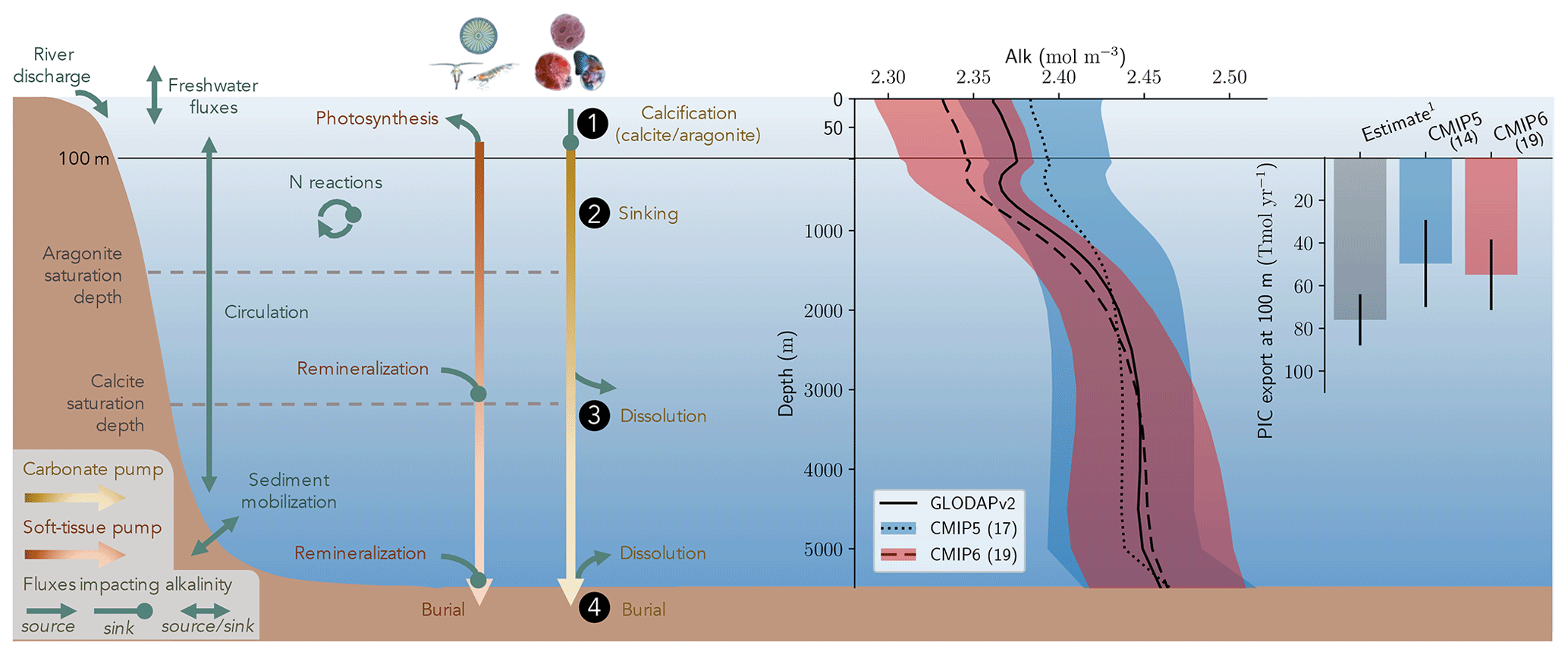
Figure 1 Schematic illustration of the processes affecting alkalinity (Alk) in the ocean highlighting the key steps of the carbonate pump addressed in this study (1, calcification, 2, sinking, 3, dissolution and 4, burial). For the CMIP5 and CMIP6 ensembles, the global-mean Alk profile and a bar chart of the total particulate inorganic carbon (PIC) export at 100 m are also presented with their associated standard deviation. Also shown are observations from GLODAPv2 for the Alk profile and the observationally derived estimate of PIC export from Sulpis et al. (2021; ¹assessment at 300 m).

2 Methodology

2.1 CMIP ESMs and their marine biogeochemical models

2.1.1 CMIP ESMs

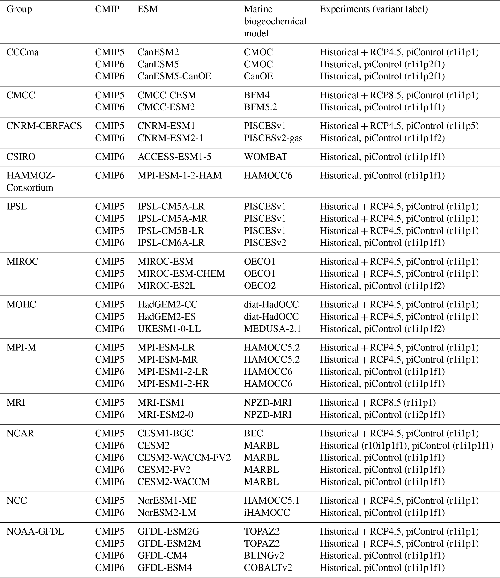
We assess 36 ESMs from 13 different climate modelling centres (CCCma, CMCC, CNRM-CERFACS, CSIRO, HAMMOZ-Consortium, IPSL, MIROC, MOHC, MPI-M, MRI, NCAR, NCC, and NOAA-GFDL), which took part in the fifth and/or sixth phases of the Climate Model Intercomparison Project (CMIP5, Taylor et al., 2012; CMIP6, Eyring et al., 2016). We only consider ESMs for which Alk is not prescribed but determined by physical and biogeochemical processes represented in the models (e.g. calcification and dissolution, or also primary production and remineralization). This leads us to include 17 ESMs for CMIP5 and 19 for CMIP6 (Table 1). In this study, we use “[ESM_name] (CMIP[number])” to refer to a given ESM, indicating whether it was used for CMIP5 or CMIP6, but we also refer to modelling centres or to the specificities of the marine biogeochemical components of the given ESMs.

In total, this ESM intercomparison encompasses 15 marine biogeochemical models (CMOC, CanOE, BFM, PISCES, WOMBAT, OECO, diat-HadOCC, MEDUSA, HAMOCC, NPZD-MRI, BEC, MARBL, TOPAZ, BLING, COBALT) with different versions and/or configurations depending on the CMIP and the modelling group. All the ESMs considered in this study represent the carbonate pump, with the exception of CMCC-CESM (CMIP5), which we include in our analysis to highlight the effect of implementing such a pump. NASA-GISS ESMs were not included as they prescribe Alk.

Table 1 Summary of the CMIP ESMs, their coupled marine biogeochemical models and the experiments assessed in this intercomparison.

2.1.2 Review of the marine biogeochemical models

We review the key properties of marine biogeochemical models simulating Alk, seeking to share an in-depth overview of the representation of the Alk tracer in these models as well as its main interior driver, the carbonate pump. Specifically, we have collected a wide range of information from the different groups, both for CMIP5 and CMIP6, regarding the protocols followed (e.g. spin-up, initialization), the model boundary conditions (e.g. river discharge, Alk restoration), and the biological complexity and representation of explicit or implicit mechanisms (e.g. CaCO₃ production, dissolution, sedimentation). In addition, we also report the nitrogen reactions taken into account by the different models, but we do not explore their effects on the Alk distribution, which can be complex under low-oxygen conditions (e.g. Stock et al., 2020). Finally, it should be noted that we were unable to collect comparable information for all models, notably the HAMMOZ-Consortium group, which is assumed to be identical to MPI-M for CMIP6 in terms of marine biogeochemistry modelling (Table 1).

2.2 ESM data and processing

2.2.1 ESM data

For the different ESMs, we systematically processed the CMIP piControl (pre-industrial control) and Historical (covering the recent past) experiments. For CMIP5, where the historical simulation covers only the time period up to 2005, we concatenated the Historical experiments with RCP4.5 (or RCP8.5 if not available) from 2005 to 2014 to allow for data averaging over 1992–2012, for consistency with observations (see Sect. 2.3). Finally, we analyse only one ensemble member per ESM (Table 1), such that we do not address the role of internal variability in the emergence of climate-related changes in the key marine biogeochemistry variables we consider in this analysis.

The following variables were processed when available: (i) two-dimensional (2D) variables: “epc100” (sinking flux of organic matter at 100 m, mol m⁻² s⁻¹), “epcalc100” (sinking flux of calcite at 100 m, mol m⁻² s⁻¹), “eparag100” (sinking flux of aragonite at 100 m, mol m⁻² s⁻¹); (ii) three-dimensional (3D) variables: “talk” (total alkalinity, mol m⁻³), “dissic” (dissolved inorganic carbon, mol m⁻³), “no3” (nitrate concentration, mol m⁻³), “po4” (phosphate concentration, mol m⁻³), “so” (salinity, g kg⁻¹), “thetao” (potential temperature, K for CMIP5 and ^∘C for CMIP6). Export values at 100 m were extracted from 3D export fields when 2D exports at 100 m were not provided using “expc” (sinking flux of organic matter, mol m⁻² s⁻¹), “expcalc” (sinking flux of calcite, mol m⁻² s⁻¹), and “exparag” (sinking flux of aragonite, mol m⁻² s⁻¹). Although modelled, export data were not available for MIROC-ESM and MIROC-ESM-CHEM (CMIP5).

2.2.2 Background processing

To facilitate the ESM intercomparison, we used Climate Data Operator (CDO) functions to regrid ESM outputs and observations. Specifically, we used distance-weighted average remapping “remapdis” to regrid the data on a regular $\mathrm{1}{}^{\circ }\times \mathrm{1}{}^{\circ }$ grid and linear-level interpolation with extrapolation “intlevelx” to regrid to the World Ocean Atlas (WOA) vertical grid with 33 depth levels up to 5500 m (even though 5500 m is not accessible for some of the CMIP5 ESMs). The mid-point of the uppermost level, which we refer to as the surface hereafter, was set to 5 m, given this is the deepest upper-ocean level among the ESMs considered. The analysis was performed in Python with the use of the Gibbs SeaWater (gsw) oceanographic toolbox for ocean property conversions. We also used mocsy 2.0 (Orr and Epitalon, 2015) to compute the ocean carbonate system over our averaging period (1992–2012) with the use of (i) Alk, DIC, phosphate (or nitrate divided by a Redfield ratio, $r_{\mathrm{N}:\mathrm{P}}=\mathrm{16}$, if not available), salinity and temperature from ESM outputs, (ii) silicate from GLODAPv2 observations (Olsen et al., 2020) as it is not included in many ESMs, and (iii) the seawater equilibrium constants recommended for best practices (Dickson et al., 2007; Orr and Epitalon, 2015). Quality control of ESM outputs led us to (i) exclude “po4” for CMCC-CESM (CMIP5) due to anomalously high values and long-term drift, and to (ii) exclude certain values at high latitudes given at 5500 m for MIROC ESMs in CMIP5 because they were not plausible and were likely affected by an error in model output processing before outputs were shared. Finally, each model is weighted in the calculation of CMIP5 and CMIP6 statistical values (mean, standard deviation, quartiles, and linear regressions) such that each modelling group has the same total contribution. Further 3D assessment of simulated variables by basin was performed through profiles, sections, and maps. Although beyond the scope of this study, these figures are provided online: https://doi.org/10.5281/zenodo.7637538.

2.2.3 Drift assessment

We did not correct for potential drift in the ESM outputs in order to maintain consistency between the internal mechanisms of the ESMs. However, the piControl simulations were assessed for drift and are discussed in Sect. 4.2.1. Using the piControl data coincident with the Historical simulation and the RCP (Representative Concentration Pathway) for CMIP5 simulations or SSP for CMIP6 simulations (250-year-long piControl simulations), we were able to assess whether the ESMs had reached a quasi steady state prior to the Historical simulation. We assessed the drift of the vertical gradients of Alk, DIC, nitrate, and phosphate between the surface and deep ocean, considering the difference between the first and last 20 years of the piControl simulations. Similarly, we also estimated the drift in surface salinity and temperature as well as the spatially integrated exports of PIC and POC at 100 m. Drift assessment was not possible for MRI-ESM1 (CMIP5) due to a lack of piControl outputs and was only carried out for DIC and Alk for CanESM2 (CMIP5) as nitrate data were unavailable.

2.2.4 Open-ocean mask

Our analysis focuses on the representation of Alk and the carbonate pump in the open ocean. Thus, most of the analysis and the associated figures consider the open ocean (defined in Appendix A) rather than the entire ocean. Indeed, our aim was to exclude coastal regions due to the coarse ESM resolution, but particularly to avoid inclusion of river discharge effects on Alk (see Sect. 2.4). The entire ocean was considered when values were integrated to compare with observationally based estimates (e.g. PIC and POC exports at 100 m). Unless otherwise specified, differences between consideration of the open ocean and the entire ocean were negligible.

2.3 Data products

We use the gridded data from the Global Ocean Data Analysis Project (GLODAP) to evaluate model performance. This database is built with bias-corrected water column bottle data – merged with CTD data for salinity – from the ocean surface to the bottom (Olsen et al., 2020). In particular, we made use of the second update of the second version of the gridded product (GLODAPv2.2020, Olsen et al. 2020), with an improved and extended coverage compared to the original second version (Lauvset et al., 2016) and the first version (Key et al., 2004), especially in the Arctic. GLODAPv2.2020 – referred to as GLODAPv2 hereafter – it contains data from 946 cruises, covering the global ocean from 1972 to 2019 with two quality controls, and adjustments to minimize severe biases. Note that we use the GLODAPv2 product that was normalized to the year 2002 for DIC to avoid biases due to the accumulation of anthropogenic carbon over the observational period. For consistency, we use nutrient fields from GLODAPv2 rather than those given by WOA, maintaining the same method for mapping the nutrients as for DIC and Alk (Lauvset et al., 2016). As modelling groups have internal protocols for sharing volumetric concentrations of their outputs (e.g. for Alk and DIC, mol m⁻³), and as most ESMs apply the incompressibility assumption for the ocean, we convert GLODAPv2 observations from gravimetric to volumetric units using a constant density of 1026 kg m⁻³ (approximately mean surface density).

To evaluate the simulated export of CaCO₃ from the upper ocean, we use the latest estimate of Sulpis et al. (2021) – although referenced to 300 m –, which is consistent with another recent estimate from Battaglia et al. (2016). While Battaglia et al. (2016) is an observationally constrained probabilistic evaluation, Sulpis et al. (2021) is an assessment from seawater chemistry and water-age data. These estimates seem to mark a point of agreement (76.0 ± 12.0 Tmol yr⁻¹ for the former and 75.0 [60.0; 87.5] Tmol yr⁻¹ for the latter) in the evaluations carried out since the late 1980s, which range from about 45 to 150 Tmol yr⁻¹ (Sulpis et al., 2021). This reflects both the sparsity and collection biases of in situ data from sediment-trap measurements and the difficulty in evaluating the contribution of CaCO₃ to the Alk budget with interpolated observations and numerical tools. To evaluate the simulated export of POC at 100 m, we compare the models to the observationally derived estimate of 558 Tmol yr⁻¹ from DeVries and Weber (2017). For simplicity, we chose to use the latest estimates in our analysis as data reference values, although large uncertainties remain for PIC and POC export from the surface ocean (∼ 50 to ∼ 150 Tmol yr⁻¹ and ∼ 300 to ∼ 1200 Tmol yr⁻¹ respectively), as discussed by Sulpis et al. (2021) and DeVries and Weber (2017). The observation-based rain ratio is 0.14 and was computed from integrated PIC and POC export values from Sulpis et al. (2021) and DeVries and Weber (2017) respectively.

2.4 Salinity normalization

As Alk is highly correlated with salinity in the upper ocean due to freshwater fluxes (e.g. precipitation, evaporation, and river discharge; Friis et al., 2003), salinity normalization is required to assess the influence of biogeochemical processes. We use the canonical normalization approach of dividing Alk and DIC values by the coincident salinity and multiplying this by a reference salinity value of 35 g kg⁻¹:

$$\begin{array}{}\text{(1)}& \left\{\begin{array}{l}\mathrm{sAlk}=\mathrm{35}\cdot \frac{\mathrm{Alk}}{S},\\ \mathrm{sDIC}=\mathrm{35}\cdot \frac{\mathrm{DIC}}{S},\end{array}\right.\end{array}$$

which gives the Alk and DIC that the considered fluid parcel would have at a salinity of 35 g kg⁻¹ (e.g. Sarmiento and Gruber, 2006; Fry et al., 2015). This approach was deemed appropriate given that our analysis is focused on the global open ocean, and therefore near-zero salinity values simulated by certain ESMs in the coastal ocean or closed seas are not taken into account. Hereafter, salinity-normalized Alk and DIC are referred to as sAlk and sDIC respectively. The influence of alternative salinity normalization techniques (Robbins, 2001; Friis et al., 2003; Carter et al., 2014; Koeve et al., 2014; Sulpis et al., 2021) on our results was assessed and found to be limited (see Appendix B).

2.5 Estimating the biological pump and related quantities

The expression and quantification of the biological carbon pump are essential to understanding the influence of biological processes on the distribution of Alk. The biological pump can be split into a soft-tissue pump associated with the production and remineralization of organic matter and the carbonate pump associated with the production and dissolution of CaCO₃. Here we define the pumps relative to the surface following Sarmiento and Gruber (2006). This is broadly equivalent to the TA^* method developed by Feely et al. (2002), which uses apparent oxygen utilization (AOU) instead of nitrate and/or phosphate concentrations. Our choice of method here was influenced by the direct availability of the nitrate and phosphate fields simulated by the ESMs (unlike AOU). Thus, we express the soft-tissue pump (δC_soft) and carbonate pump (δC_carb) as

$$\begin{array}{}\text{(2)}& {\displaystyle }\mathit{\delta }{\mathrm{C}}_{\mathrm{soft}}=r_{\mathrm{C}:\mathrm{P}}\cdot \mathit{\delta }{\mathrm{PO}}_{\mathrm{4}}^{\mathrm{3}-}=r_{\mathrm{C}:\mathrm{N}}\cdot \mathit{\delta }{\mathrm{NO}}_{\mathrm{3}}^{-},\text{(3)}& {\displaystyle }\begin{array}{rl}\mathit{\delta }{\mathrm{C}}_{\mathrm{carb}}& ={\displaystyle \frac{\mathrm{1}}{\mathrm{2}}}\left[\mathit{\delta }\mathrm{Alk}+r_{\mathrm{Nut}:\mathrm{P}}\cdot \mathit{\delta }{\mathrm{PO}}_{\mathrm{4}}^{\mathrm{3}-}\right]\\ & ={\displaystyle \frac{\mathrm{1}}{\mathrm{2}}}\left[\mathit{\delta }\mathrm{Alk}+{\displaystyle \frac{r_{\mathrm{Nut}:\mathrm{P}}}{r_{\mathrm{N}:\mathrm{P}}}}\cdot \mathit{\delta }{\mathrm{NO}}_{\mathrm{3}}^{-}\right],\end{array}\end{array}$$

where NO${}_{\mathrm{3}}^{-}$ and PO${}_{\mathrm{4}}^{\mathrm{3}-}$ respectively refer to the nitrate and phosphate concentrations, and for each tracer τ, δτ=ττ^surf is the difference between a tracer concentration and its surface value. r_C:P, r_C:N, and r_N:P are C:P, C:N, and N:P ratios, and r_Nut:P is a nutrient-to-phosphorus ratio with regards to the effect of the soft-tissue pump on Alk. The C:P ratio is model-dependent in our analysis ($r_{\mathrm{C}:\mathrm{P}}=\mathrm{106}$ for GLODAPv2 and the CMIP5/6 ensemble mean), whereas the N:P ratio is fixed ($r_{\mathrm{N}:\mathrm{P}}=\mathrm{16}$) and $r_{\mathrm{P}:\mathrm{P}}=\mathrm{1}$ by definition. We can thus infer $r_{\mathrm{Nut}:\mathrm{P}}=r_{\mathrm{N}:\mathrm{P}}+r_{\mathrm{P}:\mathrm{P}}+\mathrm{2}\cdot r_{\mathrm{S}:\mathrm{P}}=\mathrm{21.8}$, where we assume the S:P ratio at $r_{\mathrm{S}:\mathrm{P}}=\mathrm{2.4}$ for the observations (Wolf-Gladrow et al., 2007). Since the effect of sulfur is not taken into account in models, we use $r_{\mathrm{Nut}:\mathrm{P}}=r_{\mathrm{N}:\mathrm{P}}+r_{\mathrm{P}:\mathrm{P}}=\mathrm{17}$ for the ESMs (e.g. Brewer et al., 1975; Sarmiento and Gruber, 2006). This definition of the biological pump does not take into account the influence of ocean circulation. As a consequence, we limit the consideration of these pumps to horizontally averaged open-ocean regions, and the calculation with phosphate is preferred in the analysis when possible. Indeed, very low nitrate concentrations can be observed at the ocean surface in locations where significant phosphate remains. Our restriction of this calculation to open-ocean regions also reflects concerns that nutrient inputs from the ocean boundaries may also bias estimates of the pumps in coastal regions (Sarmiento and Gruber, 2006). We use the same decomposition approach for all ESMs and GLODAPv2, neglecting that (i) the soft-tissue pump has no impact on Alk in BFM4 and MEDUSA-2.0, (ii) CMCC ESMs, NOAA-GFDL ESMs (excluding GFDL-CESM4), and NCAR ESMs involved in CMIP6 have variable or various r_N:P and/or r_C:P, and (iii) CMCC for CMIP5 had no representation of the carbonate pump (see Supplement Table S1).

From this definition, it is important to highlight the dependency of the carbonate pump on the soft-tissue pump, combining Eqs. (2) and (3):

$$\begin{array}{}\text{(4)}& \mathit{\delta }{\mathrm{C}}_{\mathrm{carb}}={\displaystyle \frac{\mathrm{1}}{\mathrm{2}}}\left[\mathit{\delta }\mathrm{Alk}+{\displaystyle \frac{r_{\mathrm{Nut}:\mathrm{P}}}{r_{\mathrm{C}:\mathrm{P}}}}\cdot \mathit{\delta }{\mathrm{C}}_{\mathrm{soft}}\right].\end{array}$$

A positive soft-tissue pump value refers to net remineralization at a given depth compared to the surface and a negative value to net organic matter production. Similarly, a positive carbonate pump corresponds to net dissolution relative to the surface, while a negative value corresponds to net calcification. Net remineralization compared to the surface results in positive values for both the soft tissue and carbonate pumps, whereas net dissolution compared to the reference level results in positive values only for the carbonate pump. As highlighted by Sarmiento and Gruber (2006), δC_soft and δC_carb are “potential” pumps as they reveal the biological processes that drive the distribution of sAlk within the ocean but fail to account for the indirect effect of biology on air–sea CO₂ fluxes.

Alk and the carbonate cycle are closely linked due to the effect of calcification and dissolution, but the soft-tissue pump also impacts Alk. To estimate the drivers of ESM sAlk vertical profile biases in the open ocean, we decompose sAlk. We start by differentiating sAlk:

$$\begin{array}{}\text{(5)}& \mathrm{ds}\mathrm{Alk}=\mathrm{35}\cdot {\displaystyle \frac{\mathrm{dAlk}\cdot S-\mathrm{Alk}\cdot \mathrm{d}S}{S^{\mathrm{2}}}}.\end{array}$$

Rewriting Eqs. (3) and (4), δAlk can be expressed in terms of the carbonate and soft-tissue pumps:

$$\begin{array}{}\text{(6)}& \begin{array}{rl}\mathit{\delta }\mathrm{Alk}& =\mathrm{2}\cdot \mathit{\delta }{\mathrm{C}}_{\mathrm{carb}}-r_{\mathrm{Nut}:\mathrm{P}}\cdot \mathit{\delta }{\mathrm{PO}}_{\mathrm{4}}^{\mathrm{3}-}\\ & =\mathrm{2}\cdot \mathit{\delta }{\mathrm{C}}_{\mathrm{carb}}-{\displaystyle \frac{r_{\mathrm{Nut}:\mathrm{P}}}{r_{\mathrm{C}:\mathrm{P}}}}\cdot \mathit{\delta }{\mathrm{C}}_{\mathrm{soft}}.\end{array}\end{array}$$

This means that, at a given depth z, Alk can be expressed as follows:

$$\begin{array}{}\text{(7)}& \mathrm{Alk}\left(z\right)={\mathrm{Alk}}^{\mathrm{surf}}+\mathrm{2}\cdot \mathit{\delta }{\mathrm{C}}_{\mathrm{carb}}\left(z\right)-{\displaystyle \frac{r_{\mathrm{Nut}:\mathrm{P}}}{r_{\mathrm{C}:\mathrm{P}}}}\cdot \mathit{\delta }{\mathrm{C}}_{\mathrm{soft}}\left(z\right),\end{array}$$

where Alk^surf refers to the surface Alk. Combining Eqs. (7) and (5), this results in

$$\begin{array}{}\text{(8)}& \begin{array}{rl}\mathrm{ds}\mathrm{Alk}& =\mathrm{35}\cdot [{\displaystyle \frac{\mathrm{1}}{S}}\cdot {\mathrm{dAlk}}^{\mathrm{surf}}-{\displaystyle \frac{\mathrm{Alk}}{S^{\mathrm{2}}}}\cdot \mathrm{d}S+{\displaystyle \frac{\mathrm{1}}{S}}\cdot \mathrm{2}\cdot \mathrm{d}\mathit{\delta }{\mathrm{C}}_{\mathrm{carb}}\\ & -{\displaystyle \frac{\mathrm{1}}{S}}\cdot {\displaystyle \frac{r_{\mathrm{Nut}:\mathrm{P}}}{r_{\mathrm{C}:\mathrm{P}}}}\cdot \mathrm{d}\mathit{\delta }{\mathrm{C}}_{\mathrm{soft}}],\end{array}\end{array}$$

distinguishing four terms related to the role of surface Alk, salinity, and both the carbonate and soft-tissue pumps. Using the operator Δ defined on a tracer τ by $\mathrm{\Delta }\mathit{\tau }={\mathit{\tau }}^{\mathrm{Simu}}-{\mathit{\tau }}^{\mathrm{Obs}}$, we can express, as a first approximation, from Eq. (8), the difference in sAlk at a given depth z between the ESMs and the observations from GLODAPv2 using a reference value at the surface:

$$\begin{array}{}\text{(9)}& \begin{array}{rl}\mathrm{\Delta }\mathrm{sAlk}\left(z\right)& ={\displaystyle \frac{\mathrm{35}}{\stackrel{\mathrm{‾}}{S}}}\cdot \mathrm{\Delta }{\mathrm{Alk}}^{\mathrm{surf}}-\mathrm{35}\cdot \left({\displaystyle \frac{\stackrel{\mathrm{‾}}{\mathrm{Alk}}}{S^{\mathrm{2}}}}\right)\cdot \mathrm{\Delta }S\left(z\right)\\ & +{\displaystyle \frac{\mathrm{70}}{\stackrel{\mathrm{‾}}{S}}}\cdot \mathrm{\Delta }\left(\mathit{\delta }{\mathrm{C}}_{\mathrm{carb}}\right)\left(z\right)-{\displaystyle \frac{\mathrm{35}}{\stackrel{\mathrm{‾}}{S}}}\cdot {\displaystyle \frac{r_{\mathrm{Nut}:\mathrm{P}}}{r_{\mathrm{C}:\mathrm{P}}}}\\ & \cdot \mathrm{\Delta }\left(\mathit{\delta }{\mathrm{C}}_{\mathrm{soft}}\right)\left(z\right),\end{array}\end{array}$$

where the overbar corresponds to the mean bias between the simulations and the observations. In this way, we compute a relative decomposition – since components are not fully independent (e.g. the carbonate pump is computed from the soft-tissue pump) – to compare the different terms with the observations. Although another approach was proposed by Oka (2020), our intention here is to isolate the role of the surface Alk bias, which is key in driving carbon fluxes.

3 Results

3.1 Survey of relevant model parameterizations

Our review of the representation of Alk and the carbonate pump in the ESMs leads us to share a synthesis, which allows us to compare the different models and their evolution from CMIP5 to CMIP6 (Fig. 2). Here we document the key features we have identified regarding the carbonate pump and the global Alk budget. Additional model information is provided in Fig. C1 and in Appendix C, including specific model equations and parameters. A detailed overview of the modelling schemes used by the different groups is provided in Supplement Table S1. While CMIP models generally represent the carbonate pump in a limited number of formulations, the specific details of these often vary between models.

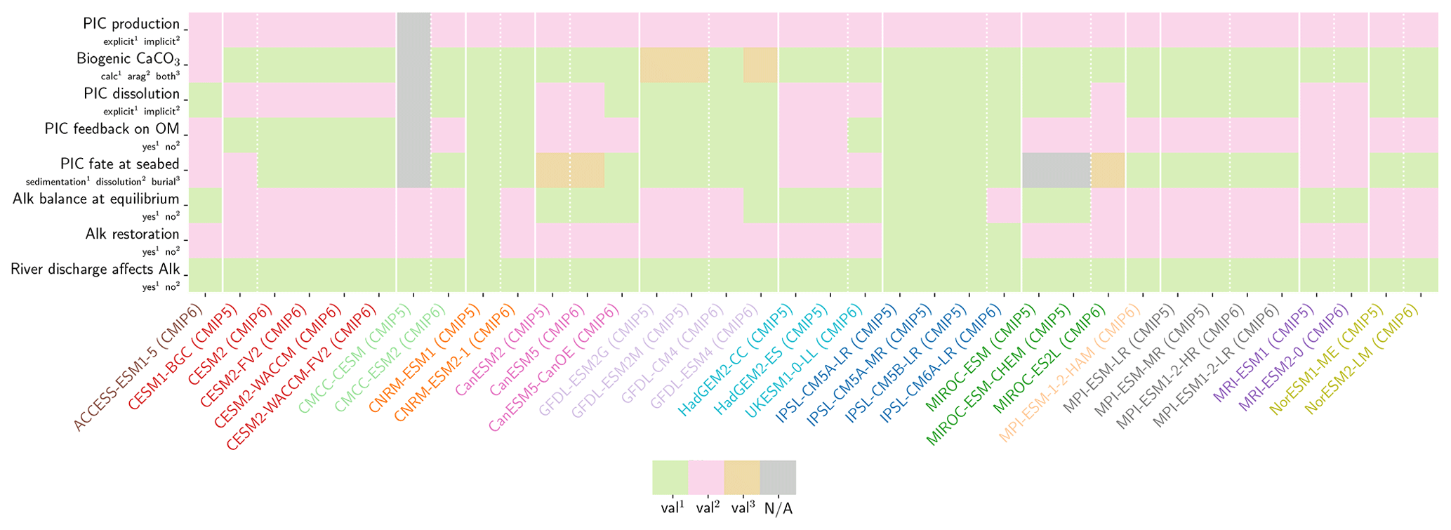
Figure 2 ESM representation of processes related to Alk and the carbonate pump. The representation and/or parameterization of each process has a subscript code associated with the potential values (1, 2, 3 or is not applicable – N/A). A more complete representation of this figure is available in Fig. C1, with further model details in Supplement Table S1.

3.1.1 Calcification

All biogeochemical models that consider the carbonate pump represent pelagic calcification implicitly in both CMIP5 and CMIP6. No model explicitly incorporates a representation of a calcifying planktonic functional type (PFT). For most of the models, biogenic CaCO₃ is in the form of calcite, although aragonite is also considered by NOAA-GFDL in TOPAZ2 and COBALTv2. Certain groups represent a generic biogenic CaCO₃ (CSIRO with WOMBAT for CMIP6, MIROC with OECO1/2 for CMIP5/6, and MOHC with diat-HadOCC for CMIP5) but attribute it either to calcite or aragonite based on their outputs and consistency with these two forms of CaCO₃ (e.g. export distribution) to conform to CMIP output requirements. Finally, we note that no model represents benthic production of CaCO₃. This reinforces the decision to focus our analysis on the open ocean and to exclude the coastal ocean when possible.

The parameterizations used to represent implicit pelagic calcification are various and show dependence on a variable number of drivers. Most of the models determine implicit calcification rates as a function of the fate of phytoplankton (through mortality and excretion by zooplankton after grazing), with certain models additionally considering the fate of zooplankton (through mortality and excretion by other zooplankton after consumption). In contrast, in CMIP5, diat-HadOCC for MOHC, OECO1 for MIROC, and TOPAZ2 for NOAA-GFDL are the only models for which calcification is directly related to phytoplankton growth. In addition, model calcification exhibits various dependencies on nutrient concentrations (phosphate, nitrate, iron, and silica), temperature, light, depth, and the calcium carbonate saturation state (Ω):

$$\begin{array}{}\text{(10)}& \mathrm{\Omega }={\displaystyle \frac{\left[{\mathrm{CO}}_{\mathrm{3}}^{\mathrm{2}-}\right]\cdot \left[{\mathrm{Ca}}^{\mathrm{2}+}\right]}{{\mathrm{K}}_{\mathrm{sp}}}}\approx {\displaystyle \frac{\left[{\mathrm{CO}}_{\mathrm{3}}^{\mathrm{2}-}\right]}{\left[{\mathrm{CO}}_{{\mathrm{3}}_{\mathrm{sat}}}^{\mathrm{2}-}\right]}},\end{array}$$

where $\left[{\mathrm{CO}}_{\mathrm{3}}^{\mathrm{2}-}\right]$ is the carbonate ion concentration, [Ca²⁺] is the calcium ion concentration – which is considered proportional to salinity – and K_sp is the apparent solubility product of CaCO₃. Ω is approximated in some models to the ratio between the carbonate ion concentration and that at saturation, $\left[{\mathrm{CO}}_{{\mathrm{3}}_{\mathrm{sat}}}^{\mathrm{2}-}\right]$. NOAA-GFDL with TOPAZ2, BLINGv2, and COBALTv2 and MOHC with MEDUSA-2.0 all consider CaCO₃ production to be dependent on the saturation state, with no calcification in undersaturated waters (Ω<1). The implicit calcification parameterizations adopted by ESMs directly relate net CaCO₃ production to the export of PIC, as opposed to gross CaCO₃ production, of which only a fraction is exported. By not explicitly resolving the grazing of calcifying plankton and partial egestion of CaCO₃ by zooplankton (e.g. due to gut dissolution), it is expected that simulated CaCO₃ production will generally be less than observational estimates of the total production of biogenic calcium carbonate.

3.1.2 Sinking and dissolution

The sinking of PIC is model-dependent, with both explicit and implicit representations in the CMIP5 and CMIP6 ensembles. When represented explicitly, a sinking speed is considered for PIC. This speed is constant in the models with the exception of PISCESv1/2(-gas), where it is depth-dependent. PIC dissolution is computed using a dissolution rate and/or a dependence on the calcium carbonate saturation state. This dependence on the saturation state is variously represented in the models. Generally, PIC dissolution in the water column occurs in undersaturated waters (Ω<1), with a linear dependence on the saturation state (BFM5.2, PISCESv2(-gas), HAMOCC5.2/6, HAMOCC5.1/iHAMOCC, TOPAZ2, and COBALTv2), although its representation is more complex in PISCESv1 and BLINGv2.

When PIC sinking and dissolution are represented implicitly, a dissolution length scale and an exponential decay of the downward flux divergence of CaCO₃ represent the combination of instantaneous sinking and dissolution in the water column. diat-HadOCC is unique in representing PIC dissolution homogeneously through the water column below a globally uniform lysocline depth – the upper limit of the transition zone, where sinking CaCO₃ starts to substantially dissolve.

3.1.3 Ballast and protection effects

In the water column, PIC can be considered both as a ballast for organic matter, increasing the sinking speed of POC, but also as a protector of organic matter reducing the rate at which it is remineralized. It is relevant to distinguishing both processes, as their feedback on the soft-tissue pump are often exclusively treated. However, what modelling groups typically consider a ballast effect is generally better described as a protection effect, as it reduces organic matter remineralization during the sinking of POC. The formulation of this process is typically based on the model proposed by Armstrong et al. (2001) in which a component of the sinking POC flux is associated with sinking CaCO₃ and experiences reduced remineralization. It is generally parameterized using the data collated by MEDUSA-2.0, BEC, MARBL, TOPAZ2, BLINGv2, and COBALTv2. PISCESv1/2(-gas) and BEC are the only models which parameterize a ballast effect. In PISCESv1/2(-gas) half of the POC produced by nanophytoplankton is associated with calcifiers and is routed to quickly sinking particles, while in BEC and MARBL a fraction of the POC is associated with the higher-dissolution length scale for “hard” particles.

3.1.4 Sedimentation and Alk sources/sinks

The fate of PIC reaching the seafloor is one of the determinants of the ocean Alk inventory and closure of the CaCO₃ budget. There is a high diversity among models in their representation of sedimentation processes associated with calcium carbonate. For some models, all of the PIC reaching the seafloor is considered permanently buried and lost from the ocean (e.g. CMOC and OECO2). Other models dissolve all of the PIC reaching the seafloor, closing the calcium carbonate cycle and avoiding its processing in the seabed (e.g. WOMBAT and NPZD-MRI). A final sub-set of models represents sediment processes. Some of these distinguish a dissolved and buried PIC fraction (e.g. CanOE, BFM5.2, and PISCES), while others represent diagenesis with a sediment module (e.g. HAMOCC, BLINGv2, and COBALTv2).

Sedimentation is one way to balance broader inputs, and especially riverine discharge that many models either ignore or represent in only simplified ways (freshwater, Alk, DIC, and nutrient discharge). At the global scale, the sedimentation of PIC at the seafloor corresponds to a net biological sink of Alk, while sediment mobilization – essentially through the dissolution of CaCO₃ present in sediments – and river discharge are a net source. Although Alk sinks and sources are ideally balanced in steady state to avoid drift in the global Alk inventory, this is difficult to achieve in certain models and is forced in others through the use of a fixed Alk inventory and a restoring term. As a result, sedimentation processes appear to be key to closing the CaCO₃ budget and are further discussed in Sect. 4.4.2.

3.2 Model performance

3.2.1 Alkalinity

The representation of surface Alk has evolved from CMIP5 to CMIP6 with a convergence of the global average value within the model ensembles, while regional disparities remain but to a lesser extent (Fig. 3). In CMIP5, the open-ocean mean surface Alk is higher than the observations (+0.022 mol m⁻³; +0.9 %), and in CMIP6 it is lower (−0.030 mol m⁻³; −1.3 %). This reflects a global decrease in surface Alk between CMIP5 and CMIP6, with an inversion of the bias relative to GLODAPv2 observations (Fig. 3 and Fig. 4a). In addition, from CMIP5 to CMIP6, the variability among the ESMs with regards to surface Alk was reduced, with a decrease in the ensemble standard deviation of surface Alk globally (from 0.057 to 0.047 mol m⁻³), and particularly in the Arctic Ocean (Fig. 3). However, in both CMIP5 and CMIP6, global-mean surface biases relative to the observations cannot be attributed to a specific and consistent regional bias among the ESMs (see Fig. D1).

Normalizing Alk by salinity (sAlk) to remove the impact of freshwater fluxes has little impact on CMIP ensemble biases (Fig. 4). Indeed, the open-ocean mean surface sAlk bias compared to observations is reversed and reduced in CMIP6 (−0.019 mol m⁻³; −0.8 %) compared to CMIP5 (+0.034 mol m⁻³; +1.4 %), and the ensemble standard deviation of surface Alk has slightly decreased (from 0.044 to 0.039 mol m⁻³; Fig. 4a). We can therefore infer that these changes are mainly driven by biogeochemical processes rather than changes in surface salinity driven by freshwater fluxes. In particular, the zonally averaged sAlk for CMIP6 is closer to observations, with an enhancement in meridional variability (Fig. 4a). This improvement between CMIP5 and CMIP6 seems to be mainly due to the elimination of some poorly performing models in CMIP6. The CNRM-CERFACS, MOHC, MIROC, and NCC ESMs in particular have a more consistent representation of the standard deviation of the sAlk surface distribution compared to observations, alongside improved correlation (Fig. 4b). However, the standard deviation of sAlk in MRI ESMs has slightly decreased from CMIP5 to CMIP6, moving away from observations, although the correlation is similar. Furthermore, there is only improvement in the correlation of sAlk in CMCC, while for IPSL the sAlk correlation is improved, but this is accompanied by an excessive increase in the surface standard deviation.

Associated with the global improvement in the representation of the surface sAlk is a significant increase in the sAlk vertical gradient (Fig. 5). The groups for which the ESMs show an improvement in the correlation and a considerable change from CMIP5 to CMIP6 in the surface sAlk standard deviation – corresponding either to an improvement (CNRM-CERFACS, MOHC, MIROC, and NCC) or a large bias (IPSL) – are the groups that reveal major improvement in the vertical profile of sAlk (Fig. 5). Indeed, from a relatively uniform sAlk profile, they now exhibit a profile with increased Alk at depth, more consistent with observations, albeit with concentrations too high. For instance, the magnitude of the sAlk vertical gradient (the concentration anomaly at 5000 m with respect to the surface) has increased from 0.02 mol m⁻³ in CMIP5 to 0.17 mol m⁻³ in CMIP6 for the IPSL ESMs, and from 0 mol m⁻³ in CMIP5 to 0.17 mol m⁻³ in CMIP6 for MOHC ESMs. The ESMs of these groups are predominantly responsible for the strengthened sAlk vertical gradient in CMIP6, which has increased from 0.05 ± 0.05 to 0.12 ± 0.05 mol m⁻³ (2.6-fold). The magnitude of the CMIP6 sAlk vertical gradient is now closer to that of the observations (0.16 mol m⁻³).

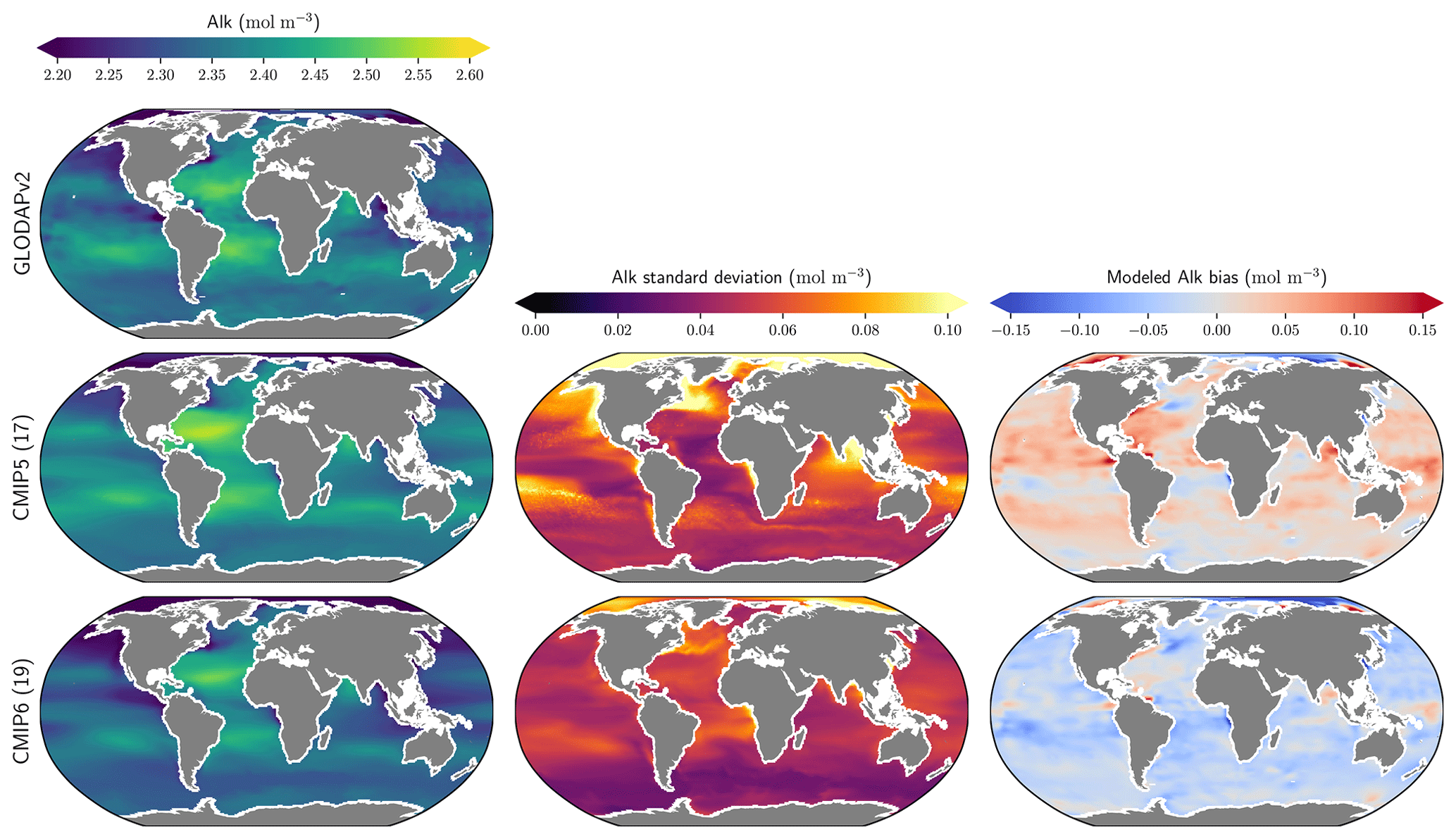
Figure 3 Alk surface distribution. The open-ocean surface Alk simulated in CMIP5 and CMIP6 compared to GLODAPv2 observations. For each CMIP ensemble, the multi-model mean, standard deviation and observational bias are shown.

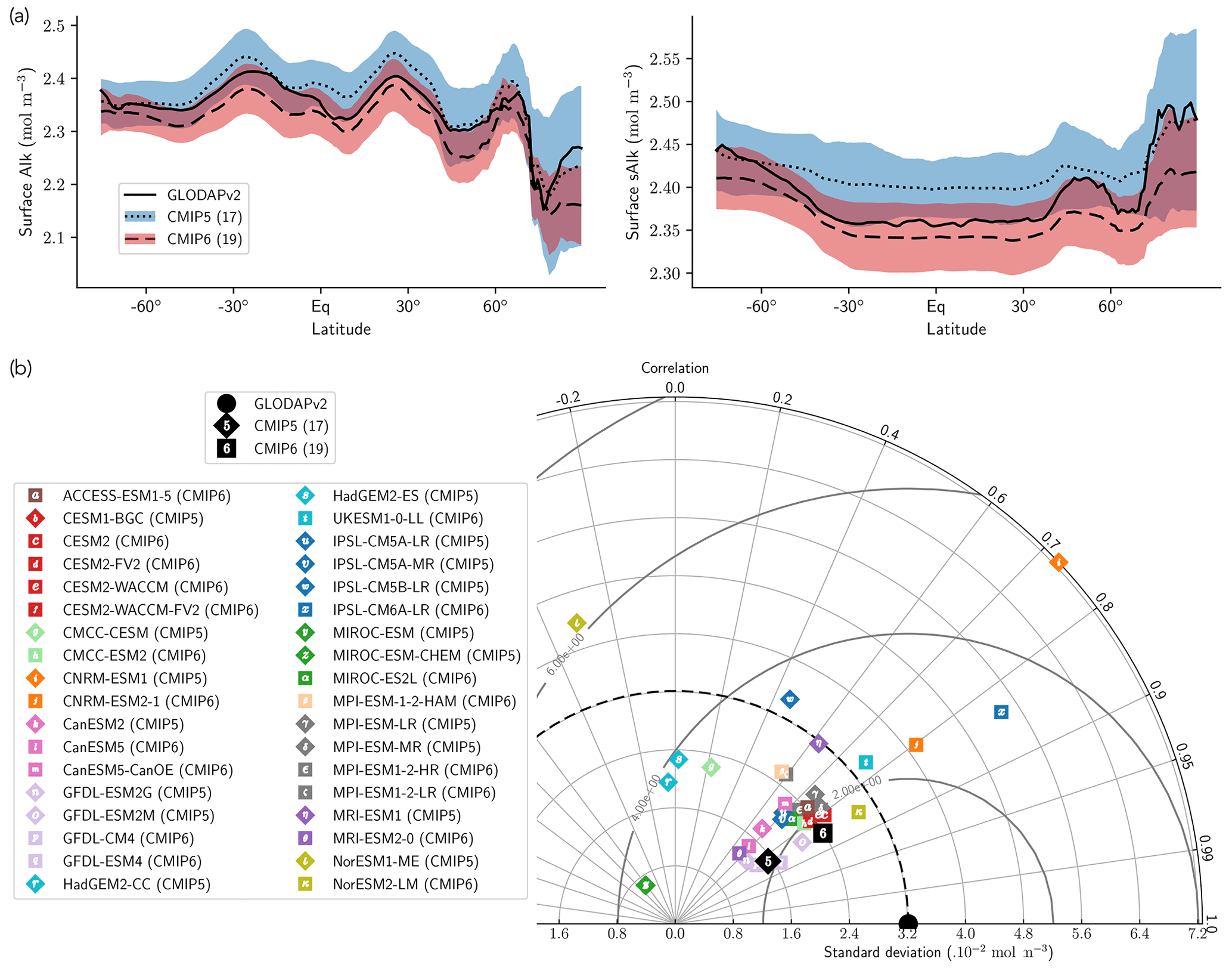
Figure 4 Spatial variability of surface Alk. (a) Open-ocean zonal mean surface Alk (left) and sAlk (right). The CMIP5 and CMIP6 ensemble mean and standard deviation are shown alongside GLODAPv2 observations. (b) Taylor diagram for the open-ocean surface distribution of sAlk. The reference corresponds to GLODAPv2 observations (black circle), and the black markers refer to the CMIP5 and CMIP6 ensemble means. The CMIP5 (CMIP6) ESMs are plotted with diamonds (squares).

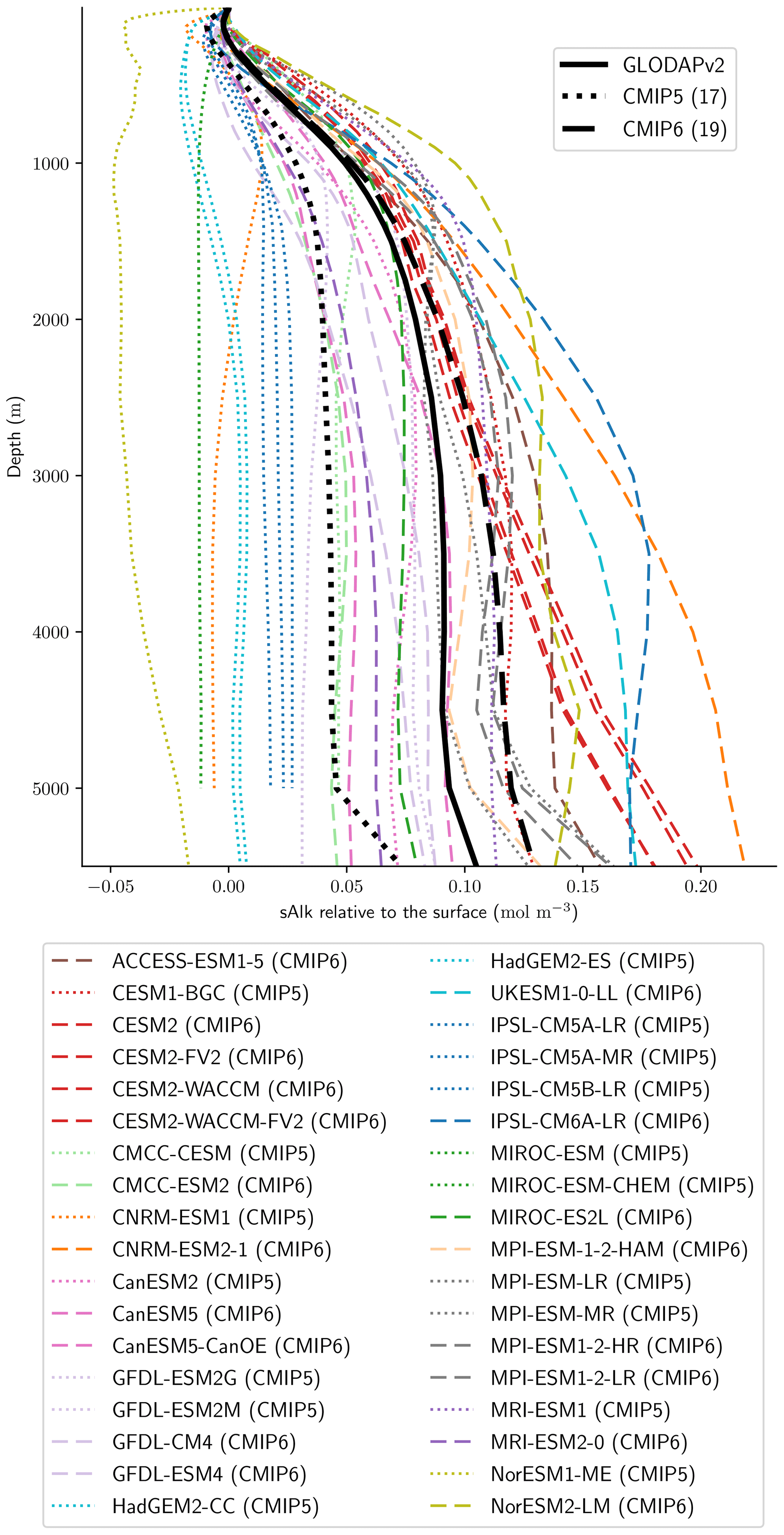
Figure 5 Global open-ocean mean sAlk vertical profile anomalies relative to surface values. The ESMs considered in this study are shown in addition to the CMIP5 (dotted) and CMIP6 (dashed) ensemble means and GLODAPv2 (solid) observations.

3.2.2 PIC export at 100 m

The global improvement in the representation of surface sAlk and the increase in the sAlk vertical gradient in CMIP6 is accompanied by an enhancement of the carbonate pump. This is illustrated by a global increase of 11 % in the PIC export at 100 m between CMIP5 (49 Tmol yr⁻¹) and CMIP6 (55 Tmol yr⁻¹; Fig. 6). Additionally, we report a decoupling in the trends from CMIP5 to CMIP6 for the PIC and POC exports, with an increase for the former and a decrease for the latter by 7 % between CMIP5 (712 Tmol yr⁻¹) and CMIP6 (659 Tmol yr⁻¹; Fig. 6). The combination of the two results in a 20 % increase in the rain ratio (RR) – defined as the ratio between PIC and POC export at 100 m (from 0.070 in CMIP5 to 0.083 in CMIP6; Fig. 6). Overall, CMIP6 ESMs tend to better match observational estimates of the exports and the RR compared to CMIP5 ESMs. While the CMIP6 average is 18 ± 27 % higher (+100 ± 151 Tmol yr⁻¹) for the POC export compared to the observationally informed estimates from DeVries and Weber (2017), it is 28 ± 26 % lower (−21 ± 20 Tmol yr⁻¹) than the estimate from Sulpis et al. (2021) for the PIC export, highlighting inter-ESM variability (Fig. 6). Although there is a global increase in the RR from CMIP5 to CMIP6, this shift is strongly associated with certain ESMs, specifically, CNRM-CERFACS and IPSL, where the increase is principally due to enhanced PIC export, and NCC, where it is due to reduced POC export (Fig. 6). While our focus is on the open ocean, when the global ocean is considered, the integrated CMIP6 mean POC and PIC exports both increase by 31 % (+155 and +13 Tmol yr⁻¹ respectively), reflecting the importance of coastal ocean export.

The spatial distribution of the RR has also evolved from CMIP5 to CMIP6, reflecting the variable trends of PIC and POC export. There is typically a greater increase in the RR at high latitudes, due to a higher increase in PIC export and a smaller decrease in POC export (see Fig. D2). There is also diversity among the ESMs with respect to the spatial distribution of PIC export at 100 m, with notable differences in the Pacific equatorial upwelling region, the great calcite belt in the Southern Ocean, and the coastal ocean (see Fig. D3 and Fig. D4). These points of disagreement between the ESMs are interestingly also found within the estimates proposed by Lee (2001), Jin et al. (2006), Sarmiento and Gruber (2006), and Battaglia et al. (2016).

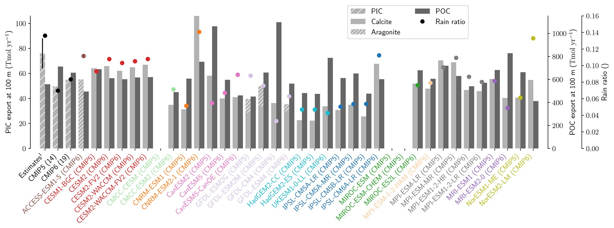
Figure 6 Export of PIC and POC at 100 m. The globally integrated PIC and POC export at 100 m (bars) and the corresponding rain ratio (points). The respective contribution of calcite and aragonite to PIC export is shown for individual ESMs. Observationally derived estimates of PIC and POC export are respectively from Sulpis et al. (2021; ¹assessment at 300 m) and DeVries and Weber (2017).

3.2.3 The carbonate pump

Using the decomposition of the sAlk bias at depth expressed in Eq. (9), we can distinguish the roles of surface Alk, salinity, the carbonate pump, and the soft-tissue pump in driving biases between the ESMs and observations at depth. The carbonate pump and surface Alk are found to explain the large majority of sAlk biases at depth (Fig. 7). Surface Alk contributes 34 % of the ensemble-mean sAlk bias at 5000 m in CMIP5 and 41 % of the bias in CMIP6, while the carbonate pump contributes 51 % of the ensemble-mean bias in CMIP5 and 46 % of the bias in CMIP6. Their respective influence has nevertheless changed from CMIP5 to CMIP6, with a greater relative contribution of surface Alk to the sAlk bias and a reduced contribution of the carbonate pump, which is further analysed in Sect. 3.3. In contrast, we find that salinity and the soft-tissue pump have a minimal influence on the sAlk bias at 5000 m in both CMIP5 and CMIP6 ensembles, contributing less than 10 %.

The CMIP6 increase in PIC export at 100 m globally acts to decrease sAlk at the ocean surface and increase it at depth. This increase could be explained by enhanced upper-ocean production and/or enhanced sinking of PIC and/or dissolution at depth. Using all the ESMs, we find a significant relationship between the sAlk vertical gradient in the open ocean and the global PIC export at 100 m (R²=0.54, p<0.01; Fig. 8a). This reflects inter-ESM consistency between higher export of PIC at 100 m and an associated increase in the vertical gradient of sAlk – expressed as the difference between the mean sAlk between 4000 and 5000 m and the mean sAlk between 5 and 100 m. In particular, it highlights the shift towards higher values of PIC export and a strengthened sAlk vertical gradient in CMIP6. The relationship encompasses the wide variety of CMIP modelling schemes used to represent Alk and the CaCO₃ cycle, despite differences in the representation of sinking, dissolution, and seabed processes. It should be noted, however, that some models clearly stand out, as is the case for UKESM1-0-LL (CMIP6) and CNRM-ESM2-1 (CMIP6). This discrepancy may be explained by the fact that for the biogeochemical scheme in UKESM1-0-LL (MEDUSA-2.1), the soft-tissue pump does not affect Alk and thus does not attenuate the sAlk vertical gradient. As for CNRM-ESM2-1 (CMIP6), very high values of the PIC export at 100 m in the Japan Sea may explain its excessive PIC export relative to the other ESMs.

The relationship established between the global sAlk vertical gradient and PIC export across the CMIP5/6 ESMs can be combined with the sAlk vertical gradient from the GLODAPv2 observations to infer PIC export at 100 m. This approach, similar to so-called “emergent constraint” methodologies (e.g. Eyring et al., 2019; Hall et al., 2019), provides a present-day PIC export estimate of 44–55 Tmol yr⁻¹ at 100 m (see the black vertical line in Fig. 8a). This estimate is lower and out of the confidence interval of PIC export values independently assessed by Sulpis et al. (2021; 76 ± 12 Tmol y⁻¹ at 300 m) and Battaglia et al. (2016; 75.0 [60.0; 87.5] Tmol yr⁻¹). This reflects an apparent underestimation of the simulated PIC export at 100 m for a given sAlk vertical gradient in comparison with observational estimates.

The sAlk vertical gradient across the combined CMIP5/6 ESM ensemble is also consistently related to the surface meridional distribution of sAlk through the Meridional Overturning Circulation (MOC) with the upwelling of Alk-enriched deep waters in the Southern Ocean. In particular, models with a higher sAlk vertical gradient have higher meridional gradients of sAlk at the surface – expressed as the difference between surface sAlk in the Southern Ocean, [−90, −45]^∘, and the low latitudes, [−45, 45]^∘ – (R²=0.46, p<0.01; Fig. 8b). Here again, the shift towards higher values for the meridional sAlk gradient and the vertical sAlk gradient from CMIP5 to CMIP6 is noticeable. Despite known differences in the representation of Southern Ocean upwelling (Beadling et al., 2020) and the spatial distribution of PIC export within the CMIP5/6 ensemble, the relationship found for the ESMs agrees relatively well with the GLODAPv2 observations.

Differences in simulated ocean circulation do not appear to be a major driver of differences in Alk gradients across the CMIP ensemble. Other factors being equal, an overly sluggish ocean circulation for instance would lead to water masses at depth that are too old and thus amplify the sAlk vertical gradient. However, using Atlantic and Southern Meridional Overturning Circulation indices (AMOC and SMOC) as proxies of the ocean overturning circulation (Heuzé et al., 2015; Heuzé, 2021), we find no robust relationship between the intensity of the global-scale ocean circulation and the sAlk vertical gradient across the CMIP ensemble.

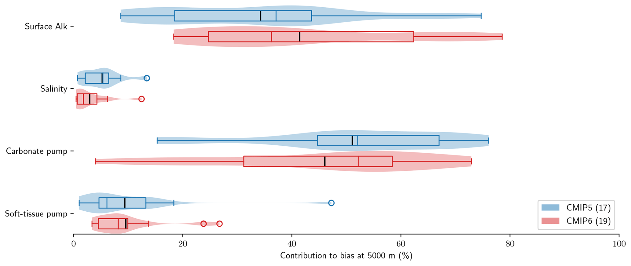
Figure 7 Relative contributions to sAlk biases between ESMs and GLODAPv2 observations at 5000 m. Violin plots of the CMIP5 and CMIP6 ensembles with the ensemble mean (black tick) and quartiles (boxes) given for each component.

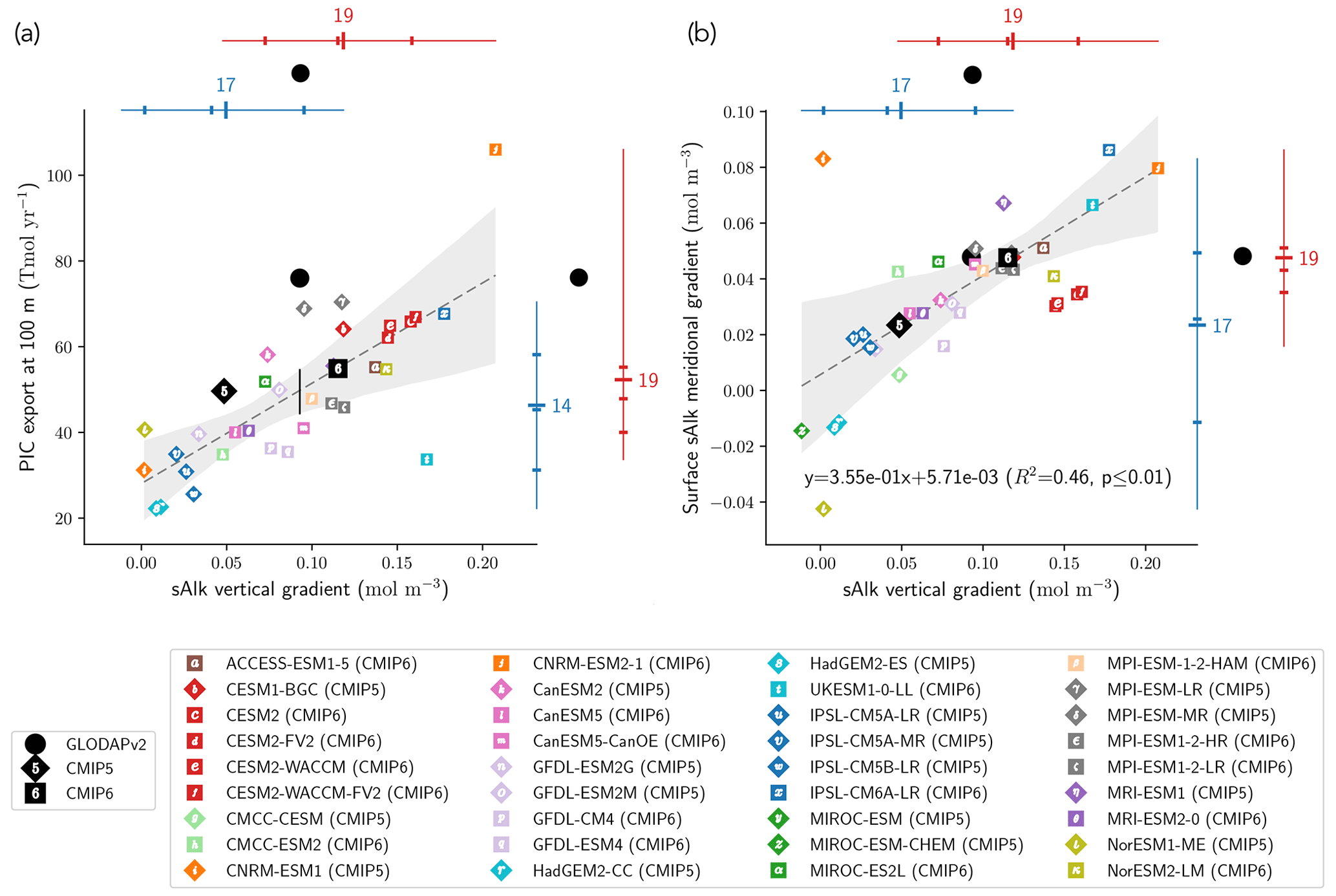
Figure 8 Relationship between the open-ocean vertical gradient of sAlk and the (a) globally integrated PIC export at 100 m and (b) surface sAlk meridional gradient between the Southern Ocean and the low latitudes. Marker notation is as in Fig. 4 with CMIP5 (CMIP6) ESMs shown as diamonds (squares). The CMIP5 (blue) and CMIP6 (red) ensemble ranges (line), mean (major tick) and quartiles (minor ticks) are displayed with the number of ESMs. GLODAPv2 observations (black circles) of the sAlk vertical gradient, combined with the estimated linear regression and 95 % confidence intervals, infer present-day global PIC export at 100 m of 44 to 55 Tmol yr⁻¹.

3.3 Pump decomposition and implications

The improvement in the representation of the carbonate pump from CMIP5 to CMIP6 strengthens the vertical gradient of sAlk but now leads to excessively low sAlk concentrations in the upper water column (including at the surface; Fig. 9a). The full decomposition of the sAlk vertical gradient into its main drivers (see Sect. 2.5) gives insights into the respective roles of the carbonate pump (analysed in Sect. 3.2.3), the soft-tissue pump, and both the surface Alk and salinity biases. The positive bias of the soft-tissue pump, present in CMIP5, has increased in CMIP6, but its influence on the sAlk bias remains limited. The use of the same r_Nut:P for the observations and ESMs (instead of 21.8 and 17 respectively; see Sect. 2.5) would have driven a minor offset in the bias associated with the carbonate pump (e.g. an sAlk bias reduction of 0.006 mol m⁻³ at 5000 m) without impacting the shape of the bias throughout the water column.

Despite the improvement in the representation of sAlk in CMIP6, the representation of the calcite and aragonite saturation horizon depth has worsened. From CMIP5 to CMIP6, a deepening of simulated saturation horizons has moved the ESMs away from observations (Fig. 9c). Moreover, although the interquartile range of simulated calcite and aragonite saturation horizons in CMIP6 is reduced compared to CMIP5, the ensemble range remains considerable. Focusing on the CMIP6 ensemble, the bias in the aragonite saturation horizon depth seems to be strongly driven by Atlantic Intermediate Water (see Fig. D6b). In contrast, the global bias for the calcite saturation depth in both CMIP5 and CMIP6 results from partial compensation between a saturation depth in the equatorial Pacific Ocean that is too shallow and a saturation depth in the North Pacific that is too deep. These regional biases showed greater global compensation in CMIP5, although the individual regional biases have been reduced in CMIP6 (see Fig. D6b). Although there is a slight deterioration in the representation of the saturation horizons from CMIP5 to CMIP6, they remain globally in broad agreement with observations. This is due to compensation between the negative biases of the respective sAlk and sDIC vertical profiles, notably in the sub-surface. The resulting vertical profile bias of sAlk–sDIC, an approximation of the carbonate ion concentration, is therefore lower than that of sAlk and sDIC (Fig. 9).

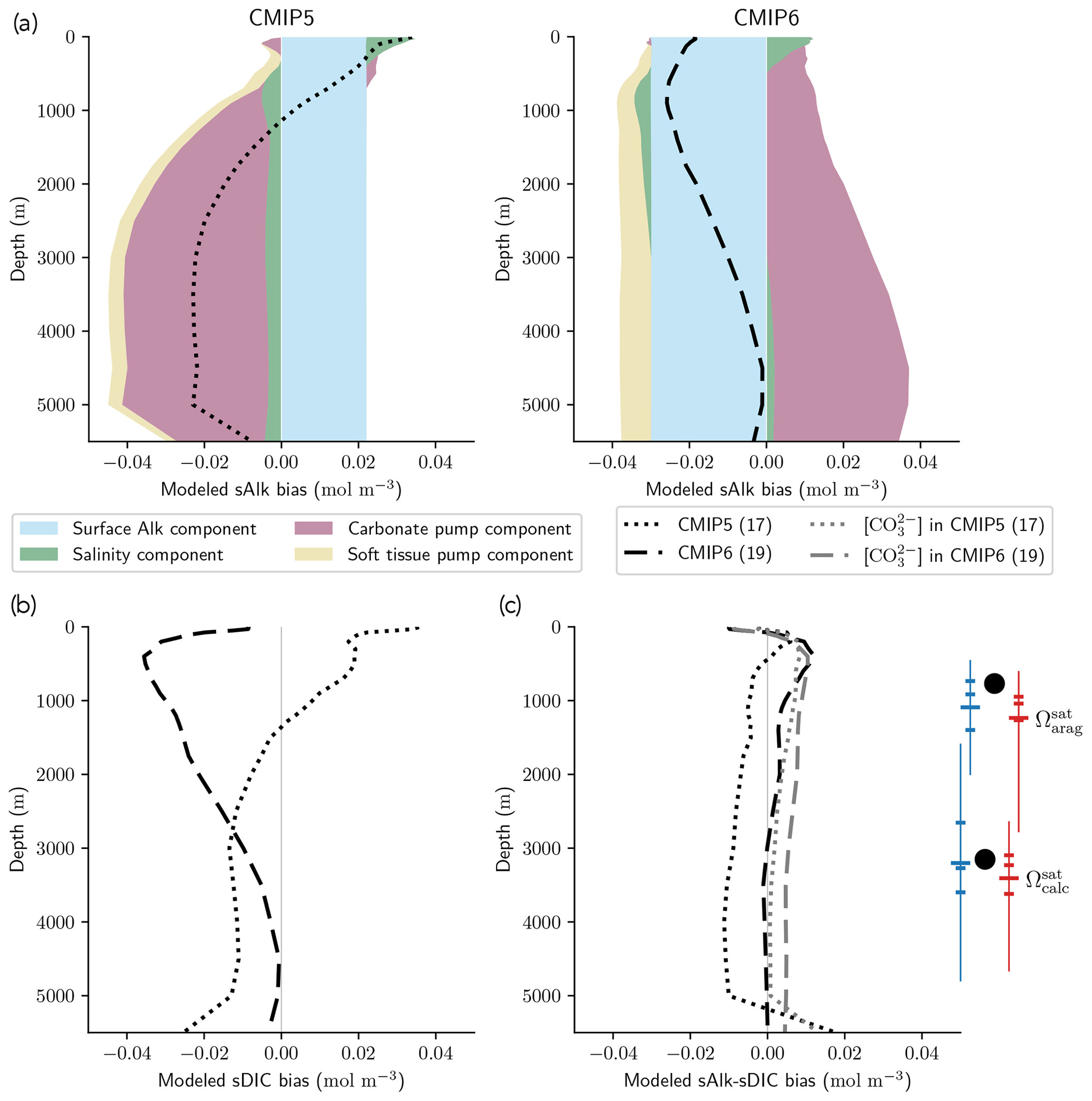
Figure 9 sAlk and sDIC vertical profile biases. (a) Decompositions of the CMIP5 and CMIP6 global sAlk vertical profile biases relative to GLODAPv2 observations. The black dotted (dashed) lines give CMIP5 (CMIP6) ensemble-mean biases. (b) sDIC and (c) sAlk–sDIC vertical profile biases for CMIP5 and CMIP6 ensemble means. The CO${}_{\mathrm{3}}^{\mathrm{2}-}$ concentration for both ensemble means is also shown in panel (c) as well as the CMIP5 (blue) and CMIP6 (red) ensemble range (line), mean (major tick) and quartiles (minor ticks) of saturation horizon depths in comparison with GLODAPv2 observations (back circles).

4 Discussion

4.1 CaCO₃ cycle model development from CMIP5 to CMIP6

In general, only limited modifications have been made with respect to the representation of the carbonate pump in the CMIP6 models compared to the respective CMIP5 versions (Fig. 2; see also Fig. C1, Appendix C, and Supplement Table S1). Such changes are insufficient to explain the increase in the intensity of the carbonate pump and in the vertical Alk profile as seen from CMIP5 to CMIP6. Although a CaCO₃ cycle has been added to the BFM biogeochemical model, in other models, parameterizations generally changed little between the two CMIP exercises. Improvements in the range of processes that can be represented with respect to the CaCO₃ cycle are limited and model-dependent. Certain ESM groups have changed their embedded ocean biogeochemical model between CMIP5 and CMIP6, with consequent changes in the CaCO₃ cycle scheme. For example, the transition from TOPAZ2 to COBALTv2, which includes enhanced resolution of the plankton food web, in NOAA-GFDL has changed the parameterization of aragonite and calcite production. One trend is towards a more complete representation of the fate of PIC at the seafloor in CMIP6 with the expansion of the use of sediment modules to at least partly balance the global ocean Alk content. This indicates that most of the model performance changes from CMIP5 to CMIP6 are likely associated with parameter tuning, or ad hoc settings, and potentially with a general increase in the horizontal and vertical model resolution and improved representation of ocean circulation (Séférian et al., 2020).

4.2 Inconsistencies in protocols and future recommendations

This analysis and review of the modelling schemes has provided insight into the protocols followed by the modelling groups and the implications this has for ESM outputs, leading us to make several recommendations for the ocean biogeochemical modelling community.

4.2.1 Drift and spin-up

The drift that we assess in the ESMs is low enough to have minimal influence on our non-drift-corrected results centred on 2002 (see Sect. 2.2.1, Fig. 10, and also Figs. D7 and D8). For instance, the model drift per century of the sAlk and sDIC vertical gradients is less than 8 % of the observed vertical gradients. Similarly, model drift in surface-ocean salinity, temperature, and exports at 100 m is also limited and should have minimal influence on the results, in part due to salinity normalization. The largest drift was observed for CMCC-CESM (CMIP5) and CNRM-ESM1 (CMIP5); specifically, the global DIC inventory of CMCC-CESM (CMIP5) had not reached equilibrium prior to the Historical simulation. In CMIP6, these two groups have increased the spin-up duration, although the relative part of their online spin-up has decreased.

There is great diversity with regards to the spin-up strategy employed by different groups (Séférian et al., 2016). Séférian et al. (2020) discussed this and pointed out that the spin-up duration has increased for all groups except IPSL and NOAA-GFDL. For these two groups, the considerable increase in resolution from CMIP5 to CMIP6 was balanced against a reduced spin-up duration as well as the completion of a fully online spin-up in the case of IPSL. Finally, we highlight two contrasting spin-up strategies with consequences for the mean ocean state of Alk and the CaCO₃ cycle. In MPI-M ESMs for CMIP5, the model was initialized with the same Alk and DIC values in all ocean grid cells and, to reduce the spin-up duration, Alk was indirectly tuned to achieve a consistent representation of the ocean CO₂ sink. This was achieved through increasing weathering fluxes and the CaCO₃ content in sediments, leading to an increase in Alk and DIC to maintain the desired pCO₂ field (Ilyina et al., 2013b). This explains the strong offset in both Alk and DIC content for MPI-M in CMIP5 (see Fig. C1). An alternative strategy was developed by NCAR for CMIP6 regarding the balancing of the global ocean budget of Alk. During the spin-up, the saturation-state threshold for the burial of CaCO₃ was tuned to balance the loss of Alk from the burial of CaCO₃ and the riverine input of Alk before starting the experimental simulations (Long et al., 2021). This resulted in the choice of an unusual threshold for the burial of CaCO₃ (see MARBL in Appendix C). Similarly, NOAA-GFDL for CMIP6 in COBALTv2 set sediment calcite concentrations such that Alk lost through calcite burial balanced river Alk inputs at a certain year during the spin-up (Dunne et al., 2012). While it is probably advisable that model groups continue to work to balance the Alk budget at quasi steady state, observations suggest there may have been a slight net sink of Alk during the Holocene and therefore potentially an ocean carbon source to the atmosphere (Ciais et al., 2013; Cartapanis et al., 2018). The strategy of maintaining a degree of freedom at the seafloor during spin-up with the tuning of parameters associated with the CaCO₃ sedimentation processes at the bottom of the ocean seems to be relevant to balancing the overall Alk budget at equilibrium. However, given the difficulty in running ESM simulations to equilibrium during the model development process, it is likely that drift correction of ocean CO₂ system variables will continue to be a requisite of robust ESM intercomparisons.

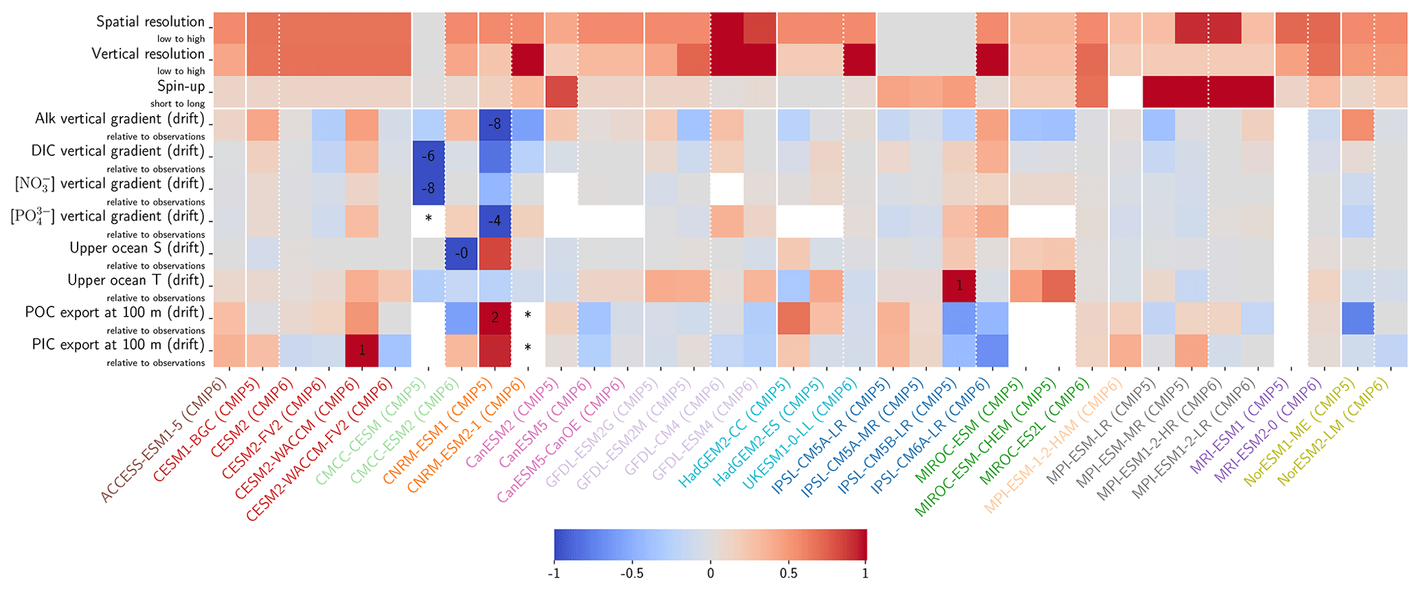
Figure 10 Resolution, spin-up and evaluation of drift in CMIP5 and CMIP6. ESM resolution and spin-up are normalized between 0 and 1, so that the highest model resolution and longest respective spin-up correspond to 1 (the maximum value attributed for the spin-up duration was set to 8000 years to keep the differences between MPI models and other ESMs visible). Model drift is normalized between −1 and 1 so that the model with the maximum absolute drift corresponds to either 1 or −1, and better-performing models have lighter cell colours. For each row, the highest model drift per century is expressed as a percentage of the observational estimate (e.g. CESM2-WACCM drift in PIC export at 100 m represents 1 % per century of observational estimates). Vertical gradients are assessed with the difference between the mean between 4000 and 5000 m and the mean between the surface and 100 m, while “upper ocean” refers to the mean between the surface and 100 m. ESMs with an issue are marked with an asterisk, and when information is missing, the cell is left blank. POC and PIC export drifts at 100 m are for the global ocean and not the open ocean, as is the case for other variables. CNRM-ESM2-1 (CMIP6) export data were not included due to extreme values in the Japan Sea, which affect the colour-scale normalization and might partly explain the model's high PIC export at 100 m (Fig. 6). Additional information on model resolution, spin-up and drift is available in Fig. C1 and Supplement Table S1.

4.2.2 Alk and DIC initialization

As previously discussed, drift can depend not only on the spin-up strategy, but also on the initialization strategy. Indeed, it is interesting to examine the initialization of Alk and DIC in ESMs and to assess how this may influence model performance. Alk and DIC fields are recommended to be initialized using the second version of the GLODAP product (GLODAPv2, Lauvset et al., 2016) following the OMIP-BGC protocol for CMIP6 (Orr et al., 2017). For CMIP5, many groups were initialized with the first gridded version (GLODAPv1, Key et al., 2004), even though this was not specific to a protocol. GLODAPv2 surface fields are more heterogeneous than GLODAPv1, but it is mainly in the coastal ocean, and in particular in the Arctic, that the two datasets diverge due to the addition of new observations. At global scale, the difference between the GLODAP products does not appear to have a noteworthy impact on the representation of both present-day Alk and DIC (Fig. 11a, b and see also Appendix E). Thus, neither the change in the GLODAP mapping method nor the increase in the number of observations is responsible for the improvement in the Alk representation from CMIP5 to CMIP6. In fact, a number of groups did not follow the OMIP-BGC protocol and instead continued using GLODAPv1 to initialize their CMIP6 models (see Supplement Table S1).

Surprisingly, it is assumptions in the conversion of the GLODAP Alk field from gravimetric to volumetric units that contribute to differences between ocean Alk distributions across ESMs. The Alk field is provided in micromoles per kilogram in the GLODAP-mapped product and must, with the exception of the NOAA-GFDL models, be converted to volumetric units (e.g. mol m⁻³) to be used by the marine biogeochemical models. Multiple approaches are employed by the groups when performing this conversion. For most of the ESMs, the conversion was made using a constant seawater density, which itself varies between ESMs (from 1024 kg m⁻³ for ACCESS-ESM1-5 (CMIP6) to 1028 kg m⁻³ for CNRM-CERFACS, IPSL, and MIROC) with in situ density used by the other ESMs (see Fig. C1). Further investigation reveals that the method of volumetric conversion for the initial Alk field drives a surface Alk bias that influences both surface DIC concentrations and the global DIC content of the ocean. Although this bias in the initialization is confined to depth depending on the density used for the conversion (see in situ, potential, and 1026 kg m⁻³ in Fig. 11c), it results in a perturbed surface-ocean CO₂ system once the ESM reaches a quasi steady state. Indeed, in an ocean with a conservative Alk inventory, the biological pump and in particular the carbonate pump only influence the distribution of Alk. Whatever the initialization of ocean DIC, the Alk content of the ocean is fixed at its initial value, and its gradient is determined through biogeochemical and physical processes. This means that surface Alk after spin-up can be inferred from the initialization field and the biogeochemical processes and ocean dynamics represented within a model. As a result, without taking into account salinity and temperature, the equilibrium between surface Alk, DIC, and atmospheric pCO₂ tends to set the surface DIC concentration at the end of spin-up through air–sea carbon fluxes. The global content of DIC is therefore directly impacted by surface Alk after spin-up with an atmosphere considered an infinite carbon reservoir. Finally, although the NOAA-GFDL models avoid initialization issues by keeping tracers in gravimetric units, the use of a constant density of 1035 kg m⁻³ during post-processing to produce “talk” and “dissic” fields distorts the ocean CO₂ system from the real ESM outputs, in particular with excessive surface values (see Fig. D1).

In addition to correct initialization of the global Alk inventory, initialization with a spatial Alk distribution consistent with observations is also required to allow accurate computation of the ocean CO₂ system and likely air–sea carbon fluxes (see mocsy 2.0; Orr and Epitalon, 2015). Indeed, the ocean biogeochemical models are generally only able to directly affect the alkalinity components associated with carbonates, phosphates, and sometimes silicates, while the other components are computed from pH (water alkalinity), salinity (fluoride alkalinity), or both (borate; Uppström, 1974; Lee et al., 2010). Thus, an inaccurate initialization of the Alk distribution (e.g. for groups initializing with a constant density) could indirectly repartition Alk between its different components, including those not directly affected by biogeochemical processes in the models. The influence of even small biases in borate alkalinity has been shown to have non-negligible effects on the ocean CO₂ system (Orr and Epitalon, 2015).

In summary, standardizing the Alk initialization protocol in CMIP exercises would reduce biases in the representation of ocean carbonate chemistry, especially at the surface. As ocean models typically apply an incompressibility assumption, it is meaningful to initialize the Alk field with the constant reference density of a given model. While a density of 1026 kg m⁻³ enables models to reproduce surface Alk values consistent with observations, the use of 1035 kg m⁻³ conserves the total alkalinity budget. However, the use of a constant density partly flattens the Alk spatial distribution, entailing potential biases. This could be partly counterbalanced by using potential density, which has a typical profile close to a constant value while maintaining spatial variability. As a consequence, we recommend initializing the Alk field with a weighted potential density in order to keep the density of reference considered within the ocean model as the mean density while being in agreement with the physical assumptions made in the models. We advise doing the same for DIC initialization.

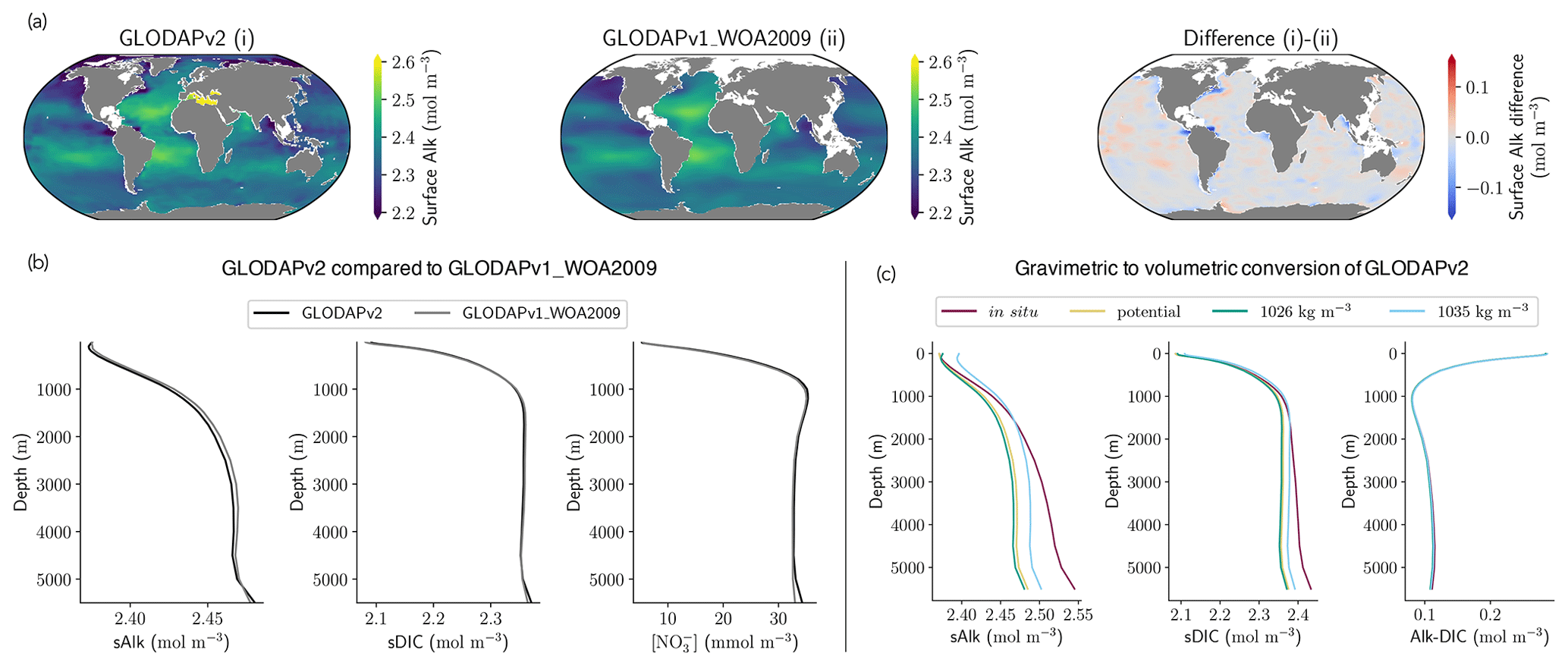
Figure 11 Influence of the observational data product and the Alk and DIC conversion strategy. (a) Maps of surface-ocean Alk for (i) GLODAPv2, (ii) GLODAPv1_WOA2009, and their difference (i)–(ii). (b) GLODAPv2 and GLODAPv1_WOA2009 vertical profiles of sAlk, sDIC, and nitrate concentration for the open ocean. (c) Vertical profiles of sAlk, sDIC, and Alk–DIC for the open ocean, with gravimetric GLODAPv2 data converted into volumetric units using either in situ density, potential density, or a constant density of 1026 kg m⁻³ or 1035 kg m⁻³.

4.2.3 Improving model assessment and traceability

The different strategies for initializing Alk and DIC highlight the importance of clear data sharing and precise protocols to enable robust ESM assessments and intercomparisons. In the following, we recommend increasing the priority of certain variables in CMIP exercises (Orr et al., 2017). First, we suggest that, in future intercomparisons, model groups share the three-dimensional export of POC and PIC (“expc”, “expcalc”, and “exparag”) and not only the exports at 100 m, as some groups have done for CMIP6. This would enable a more consistent estimate of POC and PIC export as well as the resulting rain ratio. Similarly, the potential inaccuracy of soft-tissue pump estimates based on fixed-depth POC export is well-known (e.g. Buesseler et al., 2020; Koeve et al., 2020). The simulated increase in sDIC in the upper 100 m of the water column, despite a relatively consistent sAlk, indicates that net remineralization of POC is occurring in much shallower waters than net dissolution of PIC in the ESMs. As such, POC export values should be used with caution when assessing rain ratios (see Figs. 6 and D2). Sharing of complete export fields would ideally be accompanied by three-dimensional fields of remineralization and dissolution (“remoc”, “dcalc”, and “darag”) to facilitate analysis of processes such as the biological pump throughout the water column. Finally, sharing of vertically integrated calcite and aragonite production (“intpcalcite” and “intparag”) and POC and PIC burial (“froc” and “fric”) would also improve assessments of the influence of the biological pump on vertical DIC and Alk profiles (see Fig. 9a, b).

Alongside the absence of certain model outputs, one issue that has presented itself throughout our analysis is a lack of model traceability between CMIP5 and CMIP6. In the absence of publications documenting model changes, it is typically not possible to trace ocean biogeochemical model developments without contacting individual developers and in certain instances asking for the model code. To address this, we propose that developers utilize a common online platform to share their code and provide an associated model guide. Such a platform would critically improve model traceability, enhancing ocean biogeochemical model transparency and accessibility (e.g. sharing river discharge values for both Alk and DIC). Within this context, the Earth System Documentation (ES-DOC, https://es-doc.org, last access: February 2022) project is highly relevant. However, in its current form, the tool is broadly insufficient for specific studies due to the paucity of ESMs participating and the level of model documentation provided.

4.3 Model intercomparison and model–data comparison

Alk is sensitive to the density used to convert from gravimetric to volumetric concentrations. Using in situ density rather than potential density increases global-mean Alk and DIC volumetric concentrations by only 1 % (+0.023 mol m⁻³ for Alk and +0.022 mol m⁻³ for DIC), but the vertical gradient of sAlk between the surface and 5500 m increases by 32 % compared to 15 % for sDIC (Fig. 11c), while this conversion has negligible effects on nitrate and phosphate.

Concentrations output by models assuming incompressibility can be considered “potential” concentrations and not “true” concentrations. The format of data sharing does not currently allow this distinction to be made. Indeed, ocean models used in CMIP exercises, which assume incompressibility, represent concentrations defined from the reference density used in the model. Thus, in order to convert modelled concentrations from volumetric to gravimetric units, the respective model reference densities should be used.

Conversion between gravimetric and volumetric concentrations can lead to biases in model intercomparisons. The use of different model reference values across an ESM ensemble results in biases unrelated to model processes when comparing “potential” concentrations. Similarly, the choice of density used to convert GLODAPv2 concentrations from gravimetric to volumetric units can shift values across the water column affecting model–data comparisons. It may therefore be worthwhile to document when model outputs are “potential” concentrations and to share the associated reference density. Ideally, all models would share “potential” concentrations with the same reference density, either by standardizing the reference densities used in the models or by using a multiplicative factor for the output concentrations.

4.4 Implications of the improved Alk representation in CMIP6

Although no major trend emerges in terms of the evolution from CMIP5 to CMIP6 with regards to the modelling schemes (see Sect. 4.1), there is nevertheless an improvement in the representation of Alk associated with a strengthened carbonate pump (see Fig. 1). Here we discuss the potential implications that this improvement may have for the ocean response to anthropogenic carbon emissions considering potential CO₂ feedbacks and the impact on ocean acidification projections.

4.4.1 Ocean carbon uptake and ocean acidification

In a CO₂-concentration-driven simulation, the surface Alk and DIC are directly connected to each other through equilibration via air–sea CO₂ fluxes. As a result, a modification of global-scale surface Alk has a direct effect on surface DIC (Fig. 12a). Indeed, neglecting the effect of temperature and salinity on the partial pressure of CO₂ at the ocean surface, we can differentiate pCO₂ as follows:

$$\begin{array}{}\text{(11)}& \begin{array}{rl}\mathrm{d}p{\mathrm{CO}}_{\mathrm{2}}& ={\left.{\displaystyle \frac{\partial p{\mathrm{CO}}_{\mathrm{2}}}{\partial \mathrm{Alk}}}\right|}_{\mathrm{DIC},S,T}\cdot \mathrm{dAlk}+{\left.{\displaystyle \frac{\partial p{\mathrm{CO}}_{\mathrm{2}}}{\partial \mathrm{DIC}}}\right|}_{\mathrm{Alk},S,T}\\ & \cdot \mathrm{dDIC},\end{array}\end{array}$$

where pCO₂, Alk, and DIC all refer to surface values and the partial differentials are both at fixed temperature and salinity. Rewriting the differentials “d” as the difference “Δ” between two ESMs gives

$$\begin{array}{}\text{(12)}& \begin{array}{rl}\mathrm{\Delta }\mathrm{DIC}& =-{\displaystyle \frac{\stackrel{\mathrm{‾}}{\partial p{\mathrm{CO}}_{\mathrm{2}}}}{\partial \mathrm{Alk}}}\cdot {\displaystyle \frac{\stackrel{\mathrm{‾}}{\partial \mathrm{DIC}}}{\partial p{\mathrm{CO}}_{\mathrm{2}}}}\cdot \mathrm{\Delta }\mathrm{Alk}\\ & +{\displaystyle \frac{\stackrel{\mathrm{‾}}{\partial \mathrm{DIC}}}{\partial p{\mathrm{CO}}_{\mathrm{2}}}}\cdot \mathrm{\Delta }p{\mathrm{CO}}_{\mathrm{2}},\end{array}\end{array}$$

where the overbars correspond to the mean surface-ocean values for the partial differentials. At the global scale, we can assume that, for a surface ocean in balance with atmospheric pCO₂, ΔpCO₂=0. Consequently, surface differences in Alk and DIC between two ESMs are linearly related. Approximating the carbonate ion concentration to Alk–DIC and using the expression for pCO₂ given in Sarmiento and Gruber (2006), this results at the ocean surface in

$$\begin{array}{}\text{(13)}& \mathrm{\Delta }\mathrm{DIC}\simeq {\displaystyle \frac{\mathrm{Alk}}{\mathrm{3}\cdot \mathrm{Alk}-\mathrm{2}\cdot \mathrm{DIC}}}\cdot \mathrm{\Delta }\mathrm{Alk}.\end{array}$$

Substituting the mean surface-ocean Alk and DIC of the combined CMIP5 and CMIP6 ensembles, $\mathrm{\Delta }\mathrm{DIC}\simeq \mathrm{0.81}\cdot \mathrm{\Delta }\mathrm{Alk}$, and indeed a very similar relationship between surface-ocean Alk and DIC anomalies for individual ESMs relative to CMIP5 ensemble-mean values is found ($\mathrm{\Delta }\mathrm{DIC}\simeq \mathrm{0.842}(\pm \mathrm{0.009})\cdot \mathrm{\Delta }\mathrm{Alk}$; R²=0.98, p<0.01; Fig. 12a).

This relationship between anomalies in surface Alk and DIC has implications for the wider surface-ocean CO₂ system. As the slope associated with the linear regression is less than 1, an ESM with higher surface Alk will tend to have a higher Alk–DIC and therefore a higher surface concentration of CO${}_{\mathrm{3}}^{\mathrm{2}-}$ and pH (Fig. 12a). The decrease in surface Alk from CMIP5 to CMIP6 therefore results in a slight decrease in pH and a generally lower calcite and aragonite saturation state, with the global surface-ocean carbonate ion concentration decreasing by 2.9 ± 2.7 % and up to 5 % in certain regions (Fig. 12b). As the timescale of air–sea CO₂ exchange can be approximated as being proportional to the carbonate ion concentration (Sarmiento and Gruber, 2006), other factors being equal, CMIP6 mean surface-ocean pCO₂ is likely to equilibrate faster with the atmosphere than that of CMIP5. An exception to this is the Southern Ocean, where upwelled deep waters are far from equilibrium with the atmosphere. In CMIP6, enhanced carbonate dissolution at depth results in upwelled Southern Ocean waters with a higher carbonate ion concentration, implying that Southern Ocean pCO₂ has a longer equilibration timescale. While the change in the carbonate pump from CMIP5 to CMIP6 seems to have a slight effect on the representation of the present-day ocean CO₂ system at the surface, it is likely to have negligible feedback on the projected ocean carbon sink, with an overall decrease in the Revelle factor (γ_DIC) of only 0.2 ± 1.3 % (Fig. 12b). The maximum potential influence of the carbonate pump and in turn surface Alk on the uptake of anthropogenic carbon over the historical era has previously been estimated as 5 % (Murnane et al., 1999). However, in the equatorial Pacific, where upwelling variability induced by the El Niño–Southern Oscillation (ENSO) strongly modulates surface concentrations of DIC and Alk, accurately reproducing the observed Alk vertical gradient in ESMs is important for correctly simulating the observed interannual variability of CO₂ fluxes (i.e. anomalously outgassing during El Niño and ingassing during La Niña events; Feely et al., 2006). In a recent study, Vaittinada Ayar et al. (2022) showed that the mean state of the Alk vertical profile in the tropical Pacific influences both projections of ENSO-driven CO₂ fluxes and long-term carbon uptake in the region.

Finally, the trend in surface Alk and DIC from CMIP5 to CMIP6 also influences spatial heterogeneity, especially between the low latitudes ([−40, 40]^∘) and the Southern Ocean ([−90, −40]^∘), with enhanced meridional surface gradients of Alk and DIC in CMIP6 compared to CMIP5 (+0.024 and +0.013 mol m⁻³; Fig. 13). Neglecting model differences in ocean dynamics, we can estimate that differences in the amplitude of the soft tissue and carbonate pumps between CMIP6 and CMIP5 impact the meridional surface gradients of DIC and Alk. To estimate this effect, we define an attenuation coefficient (α) as the ratio between the meridional Alk gradient at the surface (δ^{Southern-midlat}sAlk^surf) and the vertical open-ocean Alk gradient (δ^{5000 m-surf}sAlk):

$$\begin{array}{}\text{(14)}& \mathit{\alpha }={\displaystyle \frac{\begin{array}{c}{\left({\mathit{\delta }}^{\text{Southern-midlat}}{\mathrm{sAlk}}^{\mathrm{surf}}\right)}_{\mathrm{CMIP}\mathrm{6}}\\ -{\left({\mathit{\delta }}^{\text{Southern-midlat}}{\mathrm{sAlk}}^{\mathrm{surf}}\right)}_{\mathrm{CMIP}\mathrm{5}}\end{array}}{\begin{array}{c}{\left({\mathit{\delta }}^{\text{5000\hspace{0.17em}m-surf}}\mathrm{sAlk}\right)}_{\mathrm{CMIP}\mathrm{6}}\\ -{\left({\mathit{\delta }}^{\text{5000\hspace{0.17em}m-surf}}\mathrm{sAlk}\right)}_{\mathrm{CMIP}\mathrm{5}}\end{array}}}.\end{array}$$

We associate this coefficient with the upwelling that determines the vertical Alk gradient in the Southern Ocean. Hence, by multiplying the deviations of both the soft tissue and carbonate pumps at depth for CMIP6 relative to CMIP5 by this attenuation coefficient, we are able to trace the origin of the changes in the meridional gradients of Alk and DIC from CMIP5 to CMIP6 with a residual component (including the gas-exchange pump and anthropogenic carbon uptake; Fig. 13). This highlights that the increase in the carbonate pump from CMIP5 to CMIP6 is the main driver of the enhanced meridional surface gradients of Alk and DIC.

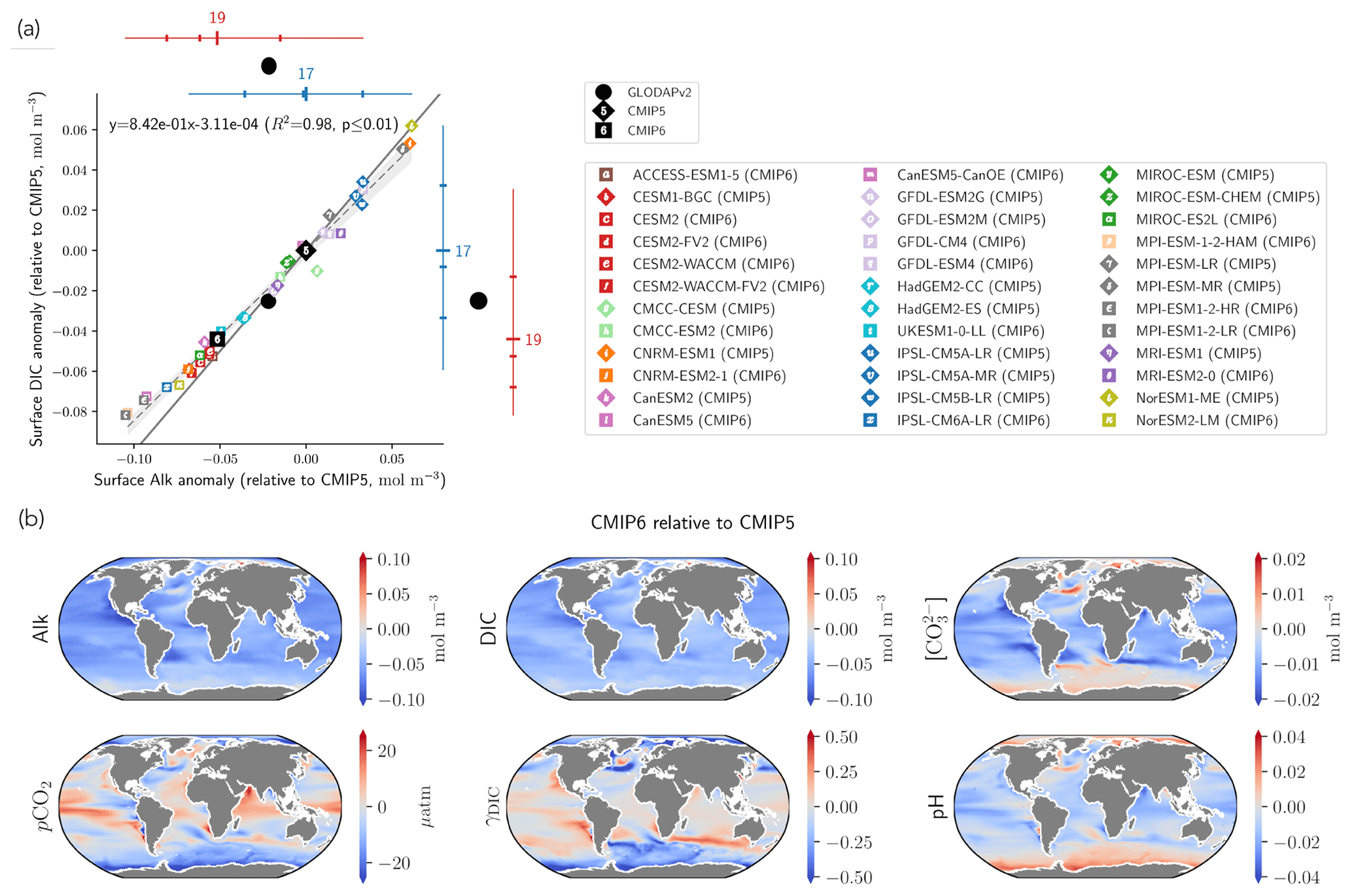
Figure 12 Surface open-ocean carbonate chemistry. (a) The relationship between mean surface-ocean Alk and DIC anomalies relative to the CMIP5 ensemble mean. The legend is the same as in Figs. 4 and 8, with the CMIP5 (CMIP6) ESMs represented with diamonds (squares). The CMIP5 (blue) and CMIP6 (red) ensemble range (line), mean (major tick) and quartiles (minor ticks) are given with the ensemble size, and GLODAPv2 observations are shown as black circles. The dashed line is the linear regression across all ESMs, and the solid line refers to the 1:1 anomaly line (points on this line have the same Alk–DIC as the CMIP5 ensemble mean and therefore effectively the same CO${}_{\mathrm{3}}^{\mathrm{2}-}$ concentration). (b) Maps of the surface difference between the CMIP6 and CMIP5 ensemble means for carbonate system variables.

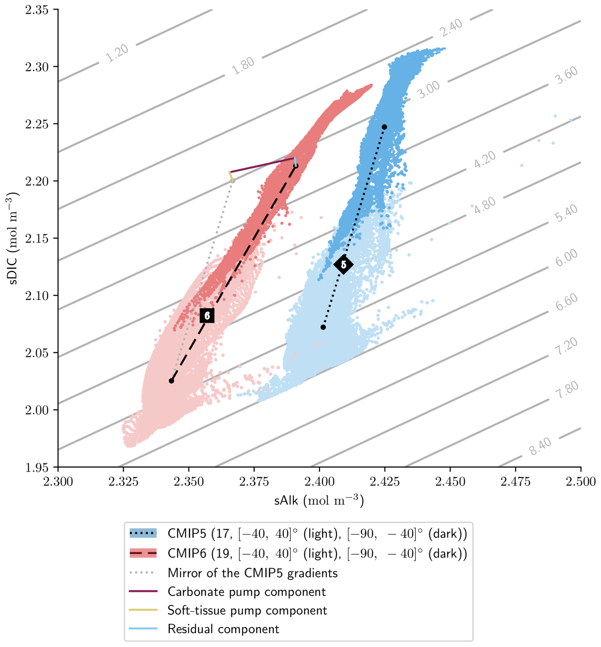
Figure 13 Scatter plot of the surface open-ocean sDIC and sAlk at low latitudes (light) and in the Southern Ocean (dark) for the CMIP5 (blue) and CMIP6 (red) ensemble means. The meridional gradient between low latitudes and the Southern Ocean mean values is shown for CMIP5 (dotted) and CMIP6 (dashed) alongside the global open-ocean mean value for CMIP5 (diamond) and CMIP6 (square). The additional lines plotted for CMIP6 give the contribution of the biological pumps and a residual component to the increase in the meridional gradient from CMIP5 to CMIP6. This highlights that the carbonate pump (purple) is the main driver of the enhanced meridional gradients of Alk and DIC. Grey background lines give the calcite saturation state calculated with mean open-ocean surface temperature, salinity, silicate and phosphate.

4.4.2 Transient changes in the ocean Alk budget and its distribution

A quasi equilibrium of Alk on centennial timescales is commonly accepted, but observational data have only recently allowed the total global Alk budget to be closed (Middelburg et al., 2020). The riverine input of Alk is mainly balanced by the burial of PIC, but also to a lesser extent by the remobilization of sediments (essentially through submarine weathering and anaerobic remineralization of organic matter) and the burial of organic matter. Interplay between these fluxes makes Alk central to the understanding of the processes driving atmospheric CO₂ over glacial and interglacial cycles (Archer and Maier-Reimer, 1994; Kerr et al., 2017; Boudreau et al., 2018). Although in modelling studies drift in the Alk inventory would impact the surface air–sea carbon flux, anthropogenic perturbation of the carbon cycle and the effect of climate change could cause transient changes in the ocean Alk inventory and its distribution. The timescales over which such perturbations may occur, and the potential consequences for projections of anthropogenic carbon uptake, are unclear.

Ocean Alk might increase through enhanced terrestrial rock weathering and an associated increase in riverine input in response to climatic drivers (e.g. enhanced precipitation, permafrost thaw; Raymond and Cole, 2003; Drake et al., 2018). In addition, shoaling of the saturation horizon due to ocean acidification is thought to explain recent observations of enhanced CaCO₃ dissolution at the seafloor (Sulpis et al., 2018) initiating chemical carbonate compensation. This highlights the potential importance of representing sediment processes in models given that CaCO₃ dissolution enriches waters in Alk and can therefore enhance ocean carbon uptake when these waters are recirculated to the surface ocean (Archer et al., 1998; Gehlen et al., 2008). Potential dissolution of coral reef CaCO₃ in response to climate change (Cooley et al., 2022) may also increase Alk on centennial timescales – echoing the coral reef hypothesis and its potential effect on atmospheric CO₂ during glacial–interglacial transitions (Berger, 1982; Opdyke and Walker, 1992).

Finally, the possibility of implementing large-scale ocean Alk enhancement (OAE, Renforth and Henderson, 2017; Bach et al., 2019) could increase the global Alk inventory on relatively short timescales. Representation of CaCO₃ burial and sub-marine weathering is necessary in simulations of OAE, even on decadal to centennial timescales, since this could entail abrupt changes. To date, OAE model studies have typically directly enhanced surface-ocean Alk (Köhler et al., 2013; Ilyina et al., 2013a; Hauck et al., 2016; González and Ilyina, 2016; Lenton et al., 2018; González et al., 2018); however, in reality Alk is likely to be provided via the addition of a mineral such as olivine, of which only a fraction will dissolve in the surface ocean. The explicit simulation of alkaline mineral addition could enhance Alk at depth, deepening the carbonate saturation horizon, suppressing the dissolution of sediment carbonate that might otherwise occur, and increasing the burial of sinking CaCO₃.

Strategies used to close the Alk budget in ESMs are questionable in simulations where the global Alk inventory may not be in quasi equilibrium (Keller et al., 2018). Indeed, in CMOC and CanOE, CaCO₃ burial at the seafloor is redissolved at the ocean surface locally to close the Alk budget. This parameterization is intended to represent fluvial Alk sources (Christian et al., 2022) but does not impact the spatial distribution of surface Alk in the same manner. It also couples riverine discharge of Alk with the carbonate pump in projections. As previously discussed, in CMIP6, NCAR and NOAA-GFDL with COBALTv2 control the Alk balance at depth by tuning the calcite saturation-state threshold for burial and the sediment calcite concentration. Similarly, IPSL and CNRM in CMIP5 with PISCESv1 force this balance at depth, not explicitly taking into account the processes at the sediment interface. Other ESMs dissolve all the PIC that reaches the seafloor in the last ocean level, effectively avoiding the consideration of an Alk burial sink (WOMBAT, BEC, diat-HadOCC, and NPZD-MRI). For the models that include a sediment module, control of the global Alk budget under pre-industrial conditions might be complicated. However, the approach used by some groups (CNRM-CERFACS and IPSL in CMIP5 and CMIP6) to restore the global Alk inventory to ensure its conservation can mask Alk budget imbalances and potentially bias Alk vertical profiles. In particular, this could lead to drifts if Alk is no longer restored after spin-up (CNRM-CERFACS in CMIP6).

4.4.3 Potential changes in the carbonate pump

An ESM representation of the carbonate pump that includes ocean acidification and climate change sensitivities has the potential to produce climate feedbacks in centennial projections. Such a model would require a relatively high level of biological realism, taking into account the complexity of the response of the CaCO₃ cycle to environmental stressors (Gattuso and Hansson, 2011; Schlunegger et al., 2019). Most studies suggest a negligible CaCO₃ cycle climate feedback this century, although on longer timescales this feedback can be more important (e.g. Gehlen et al., 2007; Ridgwell et al., 2007; Schmittner et al., 2008; Hofmann and Schellnhuber, 2009; Gangstø et al., 2011; Pinsonneault et al., 2012; Krumhardt et al., 2019). However, uncertainties and diverse responses of calcifying organisms to environmental change (e.g. Kroeker et al., 2013) make it difficult to constrain model parameterizations with confidence. Furthermore, most studies only consider a sub-set of potential impacts on the CaCO₃ cycle. Here we discuss current ESMs, highlighting developments that may affect the CaCO₃ cycle climate feedback.

Although projected ocean acidification and climate change impacts (e.g. warming and reduced upper-ocean nutrient concentrations) have diverse effects on calcification, meta-analyses generally support an expected decrease in calcification due to ocean acidification (Kroeker et al., 2013; Meyer and Riebesell, 2015; Seifert et al., 2020). This would lead to an increase in surface Alk and a decrease in Alk at depth, with possible effects on anthropogenic carbon uptake. The increased energetic cost of calcification could also impact the diversity of pelagic calcifiers and their niches (e.g. for coccolithophores; Monteiro et al., 2016). While the representation of saturation-state-dependent calcification was previously prioritized (Ridgwell et al., 2009; Gehlen et al., 2007; Gangstø et al., 2008, 2011; Hofmann and Schellnhuber, 2009; Pinsonneault et al., 2012), this is no longer the case. NOAA-GFDL and MOHC in CMIP6 are the only groups in this intercomparison to consider such a dependence. We recommend that the other groups follow their lead in improving the realism of the carbonate pump response to anthropogenic emissions.

The implicit representation of pelagic calcification in current ESMs depends on the fate of organic matter and therefore indirectly on net primary production (NPP). However, projected NPP changes this century are highly uncertain across the CMIP5/6 ensembles (Kwiatkowski et al., 2020). For all ESMs any environmental impact on planktonic calcifiers does not affect organic matter production. Moreover, changes in the growth rate of calcifiers do not impact CaCO₃ production, with the exception of BEC and MARBL, in which an implicit calcite pool is considered in the phytoplankton group. The independence and potential influence of calcifiers on organic matter production (Gattuso and Hansson, 2011) would require their explicit representation through one or more PFTs. Explicit pelagic calcifiers have been implemented in MARBL (coccolithophores; Krumhardt et al., 2019) and PlankTOM (coccolithophores, foraminifers, and pteropods; Buitenhuis et al., 2019). However, the challenge in representing both organic carbon and carbonate biomasses simultaneously is complicated by scattered observational data products (see MARine Ecosystem Model Intercomparison Project (MAREMIP) papers; O'Brien, 2012; Bednaršek et al., 2012; Schiebel and Movellan, 2012). Finally, a comprehensive representation of the carbonate pump, and thus Alk, in coastal areas, even in ESMs, will probably require the representation of benthic calcifiers as they typically dominate coastal calcification (O'Mara and Dunne, 2019; Middelburg et al., 2020). This would also be valuable within the context of climate change and ocean acidification ecosystem impact projections. CSIRO recently included benthic carbonate production for regional applications addressing the Great Barrier Reef (Steven et al., 2019), and NOAA-GFDL developed neritic environments, such as coral reefs and carbonate-rich/carbonate-poor shelves (O'Mara and Dunne, 2019). However, no benthic calcification is currently represented in ESMs. Although CaCO₃ dissolution is essentially abiotic, certain models explicitly represent the sinking of CaCO₃ with dissolution dependent on the saturation state and therefore sensitive to ocean acidification. Specifically, models represent dissolution as linearly dependent on the saturation state in undersaturated waters (see Sect. 3.1.2 and Appendix C). This is despite laboratory studies indicating an exponent >1 in the water column (most likely around 3 to 4 for calcite) while maintaining a linear dependence at the seafloor (e.g. Subhas et al., 2015; Sulpis et al., 2017; Boudreau et al., 2020). Reconciling this mismatch between laboratory results and model parameterizations would increase simulated dissolution in less undersaturated waters and thus shallower waters. This could also partially compensate for the lack of pelagic aragonite production in most models – a carbonate mineral with a lower thermodynamic stability than calcite – while the absence of simulated aragonite could influence projections of how the distribution of Alk responds to acidification. The shoaling of the saturation horizon should increase Alk at depth with a reduction in CaCO₃ burial (see Sect. 4.4.2) but also change the Alk vertical distribution with an increase in dissolution, and thus Alk, in sub-surface waters.

There is no consensus on the interaction between POC and PIC in the ocean interior with respect to a protection and/or ballast effect (see Sect. 3.1.3 and Fig. 2). Observational and laboratory data diverge (Klaas and Archer, 2002; Passow and De La Rocha, 2006; De La Rocha and Passow, 2007; Lee et al., 2009; Engel et al., 2009; Moriceau et al., 2009), highlighted by recent observations of dissolution in shallow supersaturated waters, supposedly due to POC remineralization influencing the PIC microenvironment (Subhas et al., 2022). Potential coupling between POC and PIC export may have side-effects in a transient climate change scenario with a decrease in CaCO₃ production and export, modifying organic matter remineralization (Hofmann and Schellnhuber, 2009).

Additionally, implicit PIC production avoids the representation of gross PIC production and zooplankton gut dissolution (e.g. Jansen and Wolf-Gladrow, 2001), which can potentially occur deeper than 100 m. Simulating gross PIC production and zooplankton gut dissolution may permit the representation of a sub-surface dissolution peak in addition to the deep dissolution peak seen in models with explicit saturation-state-dependent dissolution. Such a double peak in dissolution would be consistent with observations (Feely et al., 2004; Sulpis et al., 2021; Subhas et al., 2022). The representation of these two dissolution peaks may be important in the context of transient simulations as they may have different sensitivities to climate perturbations.

In order to improve the representation of the carbonate pump and to account for the impacts and feedbacks associated with acidification and climate change, certain model developments are desirable. The main priority is the parameterization of CaCO₃ production, particularly a consensus on its dependence on saturation state, temperature, and organic matter production, as this should influence the surface carbon cycle. Further desirable developments include (i) the representation of aragonite, which could partly redistribute Alk in the sub-surface and is more responsive to climate perturbations, (ii) the representation of benthic calcifiers, such as corals, which could respond on relatively short timescales, (iii) the explicit representation of saturation-state-dependent PIC dissolution, and (iv) the representation of dissolved and buried PIC fractions at the seafloor with or without the use of a diagenesis module.

5 Conclusions

Our assessment of marine biogeochemical models involved in the fifth and sixth phases of CMIP highlights the diverse representation of processes associated with the carbonate pump. CMIP6 models simulate implicit pelagic calcification, no benthic calcification and generally calcite but not aragonite. In contrast, sinking and dissolution of CaCO₃ particles are represented both implicitly and explicitly and are variably sensitive to the local seawater saturation state. The fate of PIC reaching the seafloor also differs between models due to differences in external Alk sources such as riverine fluxes and the need to conserve the global Alk inventory.

Our inter-ESM analysis reveals an improvement in the representation of the Alk distribution as compared to observations. In particular, the surface distribution and mean vertical profile of sAlk show improvements in CMIP6. This is consistent with a strengthened carbonate pump in CMIP6 resulting from a global increase in PIC export at 100 m. Despite such improvements, PIC export remains globally underestimated in the CMIP6 ensemble compared to observational estimates, while the sAlk vertical gradient is now too pronounced. The increase in the carbonate pump from CMIP5 to CMIP6 is the main driver of the reversal of the biases in the representation of the sAlk vertical profile. In addition, the shift towards lower surface values of sAlk results in lower surface values of sDIC, producing slight differences in surface-ocean carbonate chemistry between the CMIP ensembles. Specifically, the CMIP6 ESMs tend to have slightly lower surface-ocean pH and carbonate concentrations and exhibit enhanced meridional surface gradients in sAlk and sDIC. The changes in the Alk distribution in CMIP6, however, have a negligible impact on the simulated Revelle factor and therefore are likely to have little effect on the magnitude of the projected ocean carbon sink for a given emissions scenario.

An incomplete mechanistic understanding and the subsequent representation of the CaCO₃ cycle in ESMs currently limit confidence in projections of how the carbonate pump will respond to climate change and the potential climate feedback. Concerted work with biologists and observationalists is required to develop parameterizations that permit robust inter-ESM analysis of the response and feedback of the carbonate pump to projected anthropogenic emissions. This includes the development of saturation-state dependencies, benthic CaCO₃ production, and work on the coupling of PIC and POC.

Future marine biogeochemical model intercomparison projects would benefit from the provision of additional model outputs, notably three-dimensional fields of organic and inorganic export fluxes, remineralization, dissolution, integrated organic and inorganic carbon production, and PIC and POC burial. We have highlighted the need for transparency and a change in approach in studies considering Alk because of its great sensitivity to the density that is considered in converting between gravimetric and volumetric units. In particular, greater harmonization of initialization protocols with respect to Alk would avoid model biases regarding the Alk inventory and surface Alk concentrations. Finally, model traceability could be substantially improved if a shared platform were utilized to document changes to ocean biogeochemical models and the assumptions or observations underlying these developments.

Appendix A: Open-ocean mask

Throughout our analysis the open ocean was defined as >250 km from the coast, neglecting small islands (Fig. A1). This acts to (i) mask closed seas – which can have environments very different from the open ocean and are typically poorly simulated by ESMs – and (ii) maximize coincident spatial coverage in the model ensemble and observations.

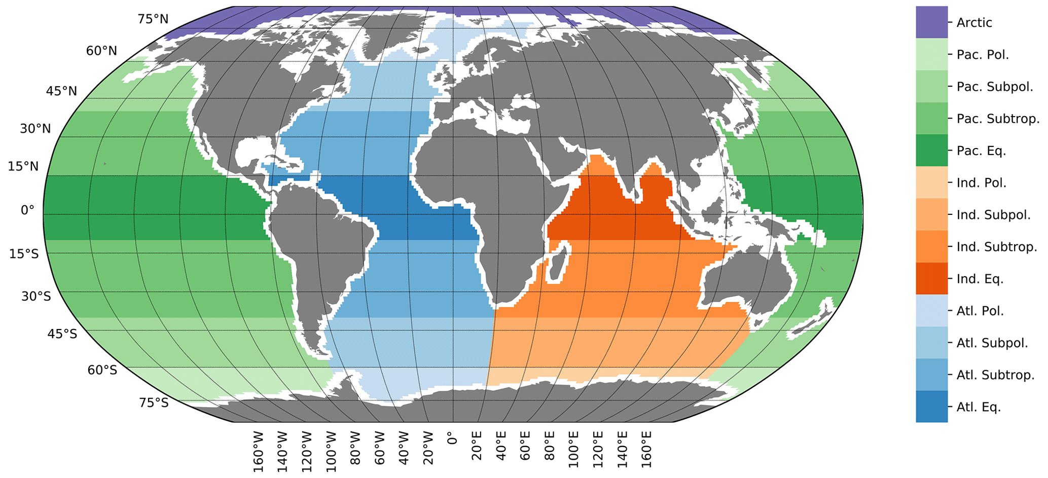
Figure A1 Map of the different ocean basins considered in the analysis: the open ocean is the coloured area at least 250 km from the coast (small islands excluded). Note that an asymmetry was considered in the tropics for the regional basins between the Southern Hemisphere and Northern Hemisphere due to the difference in the locations of the subtropical gyres.

Appendix B: Salinity normalization

The historical way to normalize Alk and DIC in the whole ocean is to divide the values by the salinity and multiply them using a salinity value of reference, generally 35 g kg⁻¹ (e.g. Postma, 1964; Millero et al., 1998). This strategy, which we employed, gives the Alk and DIC that would have the considered fluid parcel at a salinity of 35 g kg⁻¹ (e.g. Sarmiento and Gruber, 2006; Fry et al., 2015). The errors associated with this strategy are essentially confined in the ocean mixed layer where evaporation and precipitation occur (Friis et al., 2003). However, other salinity normalization techniques have been developed ever since (Millero et al., 1998; Robbins, 2001; Friis et al., 2003; Lee et al., 2006; Carter et al., 2014) on the basis of observation-based relationships between surface salinity and Alk.

In order to assess the potential biases of the historical method that Sarmiento and Gruber (2006), Krumhardt et al. (2020), and we considered (sAlk), we compare it to the strategy developed by Robbins (2001), Friis et al. (2003), and Carter et al. (2014), also used by Sulpis et al. (2021; sAlk^∗):

$$\begin{array}{}\text{(B1)}& {\displaystyle }\mathrm{sAlk}=\mathrm{35}\cdot {\displaystyle \frac{\mathrm{Alk}}{S}},\text{(B2)}& {\displaystyle }{\mathrm{sAlk}}^{\ast }=\mathrm{Alk}-{\displaystyle \frac{\stackrel{\mathrm{‾}}{{\mathrm{Alk}}^{\mathrm{surf}}}}{\stackrel{\mathrm{‾}}{S^{\mathrm{surf}}}}}\cdot S,\end{array}$$

where the overbar corresponds to the mean surface value of the observations from GLODAPv2 or the CMIP5/6 ensemble mean. Hence, the method of salinity normalization was found to have a negligible impact on vertical profiles of sAlk (Fig. B1b). A slight difference between the two methods is apparent in the surface distribution of normalized Alk, particularly in the Arctic Ocean (Fig. B1c). However, the conventional salinity normalization approach was preferred throughout our analysis, as it maintains the order of magnitude of Alk, avoids empirical relationships, and is therefore easier to interpret.

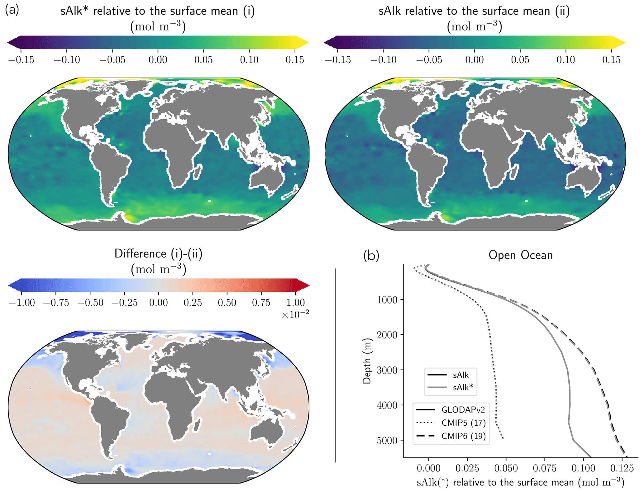
Figure B1 Evaluation of two different salinity normalization strategies. (a) Open-ocean surface sAlk^* and sAlk anomalies relative to the surface mean, and the difference. (b) Profiles of sAlk^* and sAlk for GLODAPv2 as well as CMIP5 and CMIP6 ensemble means. sAlk is defined in Sect. 2.4 and sAlk^* in Appendix B.

Appendix C: Model equations and parameters

In the following, we present the equations and parameters governing the ocean calcium carbonate cycle for each of the biogeochemical models involved in our analysis. The marine biogeochemical models are classified following Table 1, and the parameters are given in Tables C2–C19. Model non-specific variables and parameters are defined in Table C1. If processes are not included in the equations, “N/A” is given, but related information can be found in Supplement Table S1. Finally, for the PIC balance equation, a Lagrangian derivative is considered when the PIC is advected (we improperly include its diffusion in this derivative if considered) rather than a partial derivative.

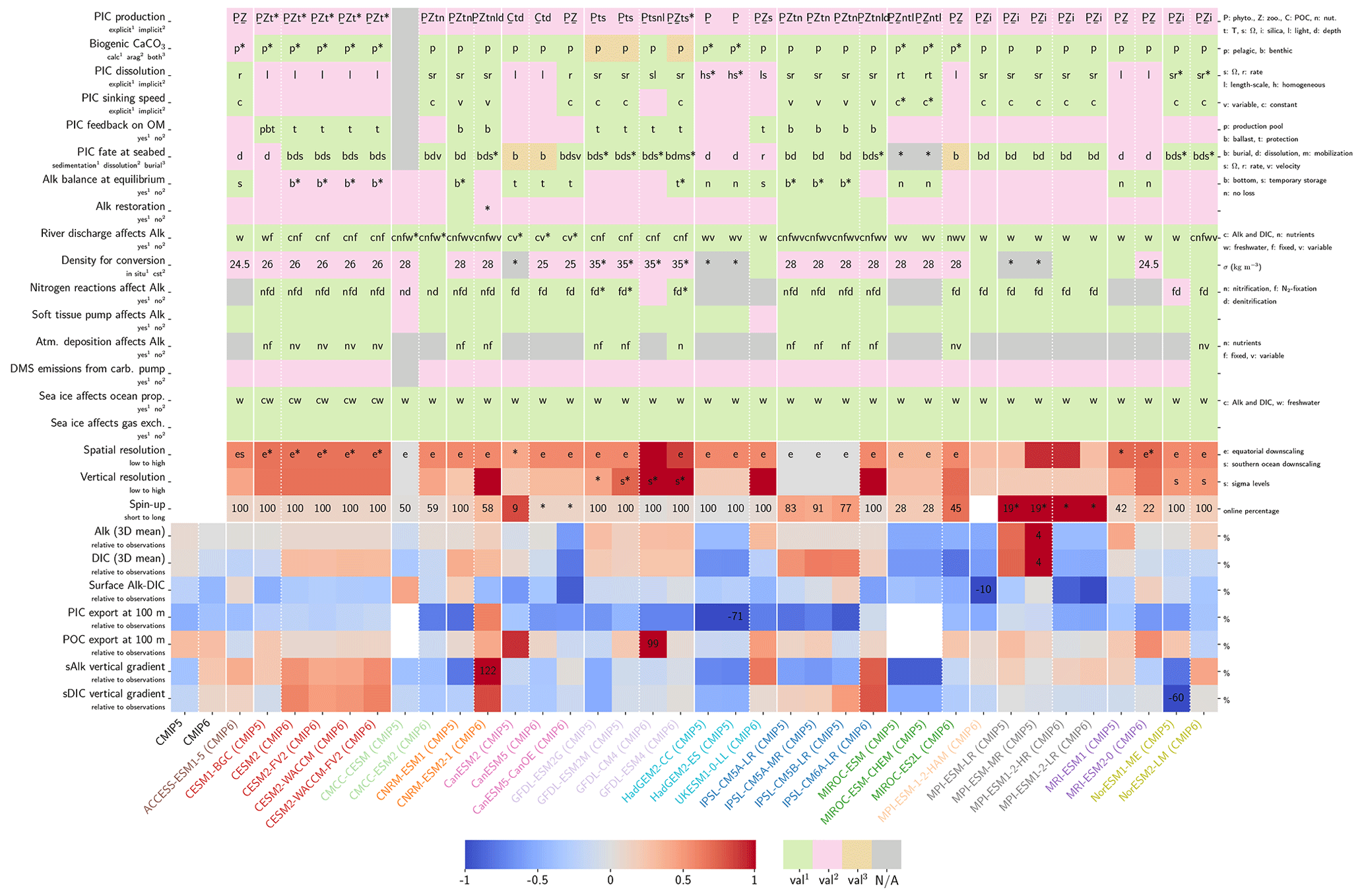
Figure C1 Model description and performance with respect to the representation of Alk and the carbonate pump (expanded from Figs. 2 and 10). Details include biogeochemical modelling schemes, resolution and spin-up, and model performance. For PIC production, underlined letters correspond to the explicitly modelled variables on which PIC production relies. Asterisks denote that further details can be found in Supplement Table S1. For the spin-up duration, the maximum value attributed was set to 8000 years to keep the differences between the other ESMs and MPI ones visible. Performance metrics are normalized between −1 and 1 so that the model with maximum absolute bias corresponds to either 1 or −1, and better-performing models have lighter cell colours. For each row, the value given for the ESM with the greatest bias corresponds to the percentage of the GLODAPv2 observational estimate that this bias represents. When information is missing, the cell is left blank.

Table C1 Definitions of general model variables and parameters.

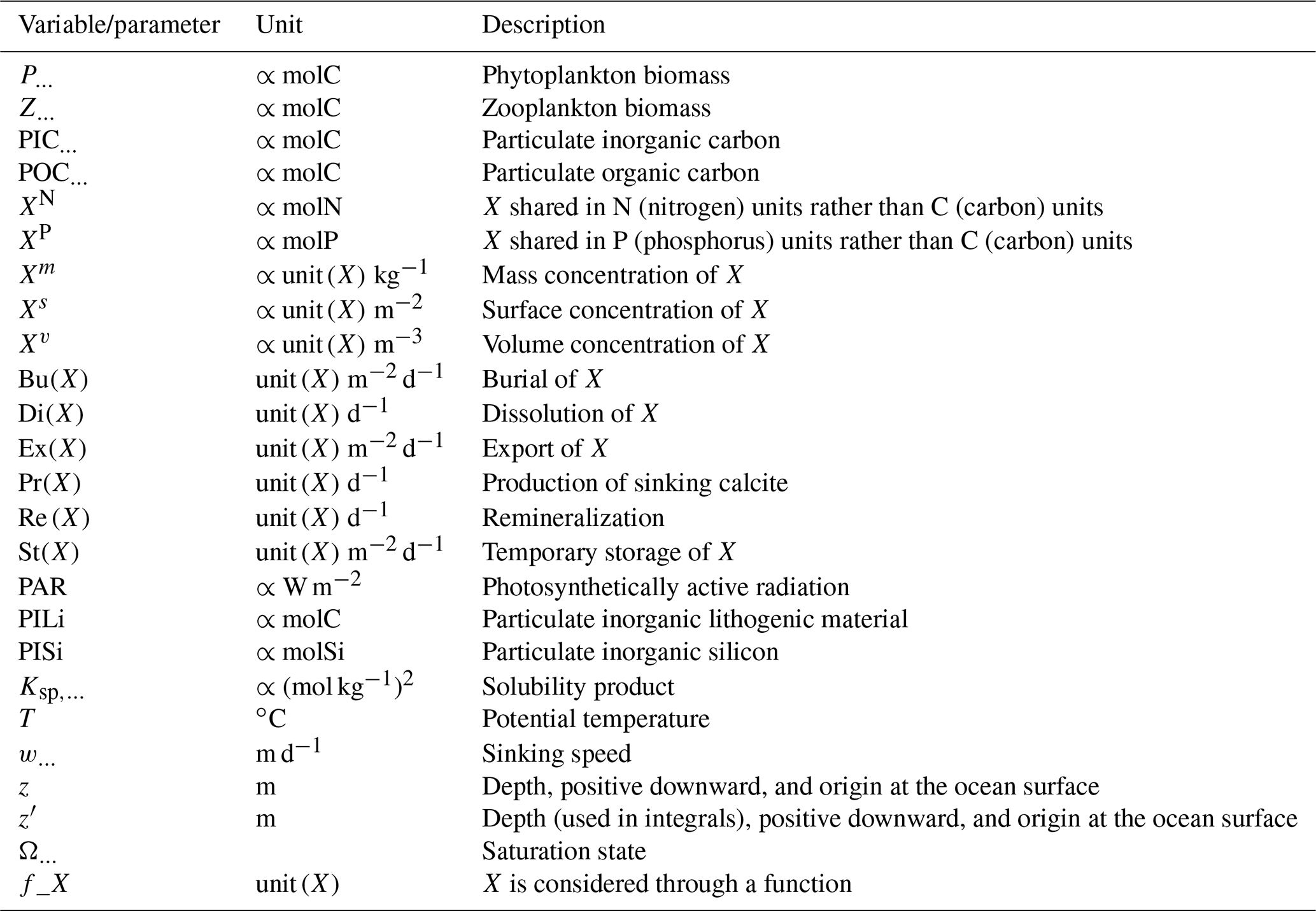
C1 CMOC

• Reference used: Zahariev et al. (2008)

• Marine biogeochemical model of CanESM2 (CMIP5) and CanESM5 (CMIP6)

•  

  PIC balance: N/A

•  

  PIC export at 100 m:

•  

  Ex$\left({\mathrm{PIC}}_{\mathrm{calc}}\right)\left(\mathrm{100}\right)=r_{{\mathrm{PIC}}_{\mathrm{calc}}}\cdot \frac{\exp \left[\mathrm{0.6}\cdot (T-\mathrm{10})\right]}{\mathrm{1}+\exp \left[\mathrm{0.6}\cdot (T-\mathrm{10})\right]}\cdot r_{\mathrm{C}:\mathrm{N}}\cdot w_{\mathrm{POC}}$

•  

  $\cdot {\mathrm{POC}}^{v,\mathrm{N}}\left(n_{z_{\mathrm{eld}}}^{\mathrm{above}}\right)$

•  

  PIC production: N/A

•  

  PIC sinking speed: N/A

•  

  PIC dissolution:

•  

  $\mathrm{Di}\left({\mathrm{PIC}}_{\mathrm{calc}}^v\right)=\frac{max\left(\mathrm{0},z-z_{\mathrm{eld}}\right)}{z-z_{\mathrm{eld}}}\cdot \frac{\mathrm{1}}{D_{{\mathrm{PIC}}_{\mathrm{calc}}}}\cdot \mathrm{Ex}\left({\mathrm{PIC}}_{\mathrm{calc}}\right)\left(z_{\mathrm{eld}}\right)$

•  

  $\cdot \exp \left(\frac{-z+z_{\mathrm{eld}}}{D_{{\mathrm{PIC}}_{\mathrm{calc}}}}\right)$

•  

  Ballast effect: N/A

•  

  Protection effect: N/A

•  

  PIC burial: N/A

Table C2 CMOC parameters.

C2 CanOE

• Reference used: Christian et al. (2022)

• Marine biogeochemical model of CanESM5-CanOE (CMIP6)

•  

  PIC balance:

•  

  $\frac{{\mathrm{DPIC}}_{\mathrm{calc}}^v}{\mathrm{D}t}=\mathrm{Pr}\left({\mathrm{PIC}}_{\mathrm{calc}}^v\right)-\mathrm{Di}\left({\mathrm{PIC}}_{\mathrm{calc}}^v\right)-w_{{\mathrm{PIC}}_{\mathrm{calc}}}\cdot \frac{\partial {\mathrm{PIC}}_{\mathrm{calc}}^v}{\partial z}$

•  

  PIC export at 100 m:

•  

  Ex$\left({\mathrm{PIC}}_{\mathrm{calc}}\right)\left(\mathrm{100}\right)=w_{{\mathrm{PIC}}_{\mathrm{calc}}}\cdot {\mathrm{PIC}}_{\mathrm{calc}}^v\left(\mathrm{100}\right)$

•  

  PIC production:

•  

  $\mathrm{Pr}\left({\mathrm{PIC}}_{\mathrm{calc}}^v\right)=r_{{\mathrm{PIC}}_{\mathrm{calc}}}\cdot \left[m^{{\mathrm{PZ}}_{\mathrm{small}}}\cdot \left(P_{\mathrm{small}}^v+Z_{\mathrm{small}}^v\right)+{\mathit{\mu }}^{{\mathrm{PZ}}_{\mathrm{small}}}\cdot \left({\left(P_{\mathrm{small}}^v\right)}^{\mathrm{2}}+{\left(Z_{\mathrm{small}}^v\right)}^{\mathrm{2}}\right)\right]$

•  

  PIC sinking speed: $w_{{\mathrm{PIC}}_{\mathrm{calc}}}$

•  

  PIC dissolution:

•  

  $\mathrm{Di}\left({\mathrm{PIC}}_{\mathrm{calc}}^v\right)={\mathit{\lambda }}_{{\mathrm{PIC}}_{\mathrm{calc}}}\cdot {\mathrm{PIC}}_{\mathrm{calc}}^v$

•  

  Ballast effect: N/A

•  

  Protection effect: N/A

•  

  PIC burial:

•  

  $\mathrm{Bu}\left({\mathrm{PIC}}_{\mathrm{calc}}\right)=\frac{max\left(\mathrm{0},{\mathrm{\Omega }}_{\mathrm{calc}}-\mathrm{1}\right)}{{\mathrm{\Omega }}_{\mathrm{calc}}-\mathrm{1}}\cdot w_{{\mathrm{PIC}}_{\mathrm{calc}}}\cdot {\left({\mathrm{PIC}}_{\mathrm{calc}}^v\right)}^{\mathrm{seafloor}}$

Table C3 CanOE parameters.

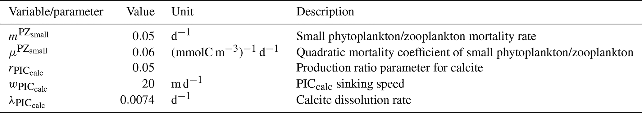
C3 BFM4

• Marine biogeochemical model of CMCC-CESM (CMIP5)

• No calcium carbonate cycle

C4 BFM5.2

• References used: Vichi et al. (2011, 2013, 2020) and Lovato et al. (2022)

• Marine biogeochemical model of CMCC-ESM2 (CMIP6)

•  

  PIC balance:

•  

  $\frac{\mathrm{D}\left({\mathrm{PIC}}_{\mathrm{calc}}^v\right)}{\mathrm{D}t}=\mathrm{Pr}\left({\mathrm{PIC}}_{\mathrm{calc}}^v\right)-\mathrm{Di}\left({\mathrm{PIC}}_{\mathrm{calc}}^v\right)-w_{{\mathrm{PIC}}_{\mathrm{calc}}}\cdot \frac{\partial {\mathrm{PIC}}_{\mathrm{calc}}^v}{\partial z}$

•  

  PIC export at 100 m:

•  

  Ex$\left({\mathrm{PIC}}_{\mathrm{calc}}\right)\left(\mathrm{100}\right)=w_{{\mathrm{PIC}}_{\mathrm{calc}}}\left(\mathrm{100}\right)\cdot {\mathrm{PIC}}_{\mathrm{calc}}^v\left(\mathrm{100}\right)$

•  

  PIC production:

•  

  $\mathrm{Pr}\left({\mathrm{PIC}}_{\mathrm{calc}}^v\right)=r_{{\mathrm{PIC}}_{\mathrm{calc}}}\cdot \left[{\mathit{\eta }}^{Z_{\mathrm{micro}}}\cdot f\mathit{\_}{\mathrm{graz}}^{Z_{\mathrm{micro}}}\cdot Z_{\mathrm{micro}}^v+\min \left(\frac{r_{\mathrm{C}:\mathrm{N}}^{P_{\mathrm{nano},\mathrm{ref}}}}{f\mathit{\_}{r}_{\mathrm{C}:\mathrm{N}}^{P_{\mathrm{nano}}}},\frac{r_{\mathrm{C}:\mathrm{P}}^{P_{\mathrm{nano},\mathrm{ref}}}}{f\mathit{\_}{r}_{\mathrm{C}:\mathrm{P}}^{P_{\mathrm{nano}}}}\right)\cdot m^{P_{\mathrm{nano},\max }}\cdot \frac{K_m^{{}^{\prime }{P}_{\mathrm{nano}}}}{\mathrm{f}\mathit{\_}{\mathrm{nut}}^{P_{\mathrm{nano}}}\cdot K_m^{{}^{\prime }{P}_{\mathrm{nano}}}}\cdot P_{\mathrm{nano}}^v\right]$

•  

  PIC sinking speed: $w_{{\mathrm{PIC}}_{\mathrm{calc}}}$

•  

  PIC dissolution:

•  

  $\mathrm{Di}\left({\mathrm{PIC}}_{\mathrm{calc}}^v\right)={\mathit{\lambda }}_{{\mathrm{PIC}}_{\mathrm{calc}}}\cdot max{\left(\mathrm{0},\mathrm{1}-{\mathrm{\Omega }}_{\mathrm{calc}}\right)}^{{\mathit{\alpha }}_{{\mathrm{PIC}}_{\mathrm{calc}}}}\cdot {\mathrm{PIC}}_{\mathrm{calc}}^v$

•  

  Ballast effect: N/A

•  

  Protection effect: N/A

•  

  PIC burial:

•  

  $\mathrm{Bu}\left({\mathrm{PIC}}_{\mathrm{calc}}\right)=w_{{\mathrm{PIC}}_{\mathrm{calc}}}^{\mathrm{seafloor}}\cdot {\left({\mathrm{PIC}}_{\mathrm{calc}}^v\right)}^{\mathrm{seafloor}}$

Table C4 BFM5.2 parameters.

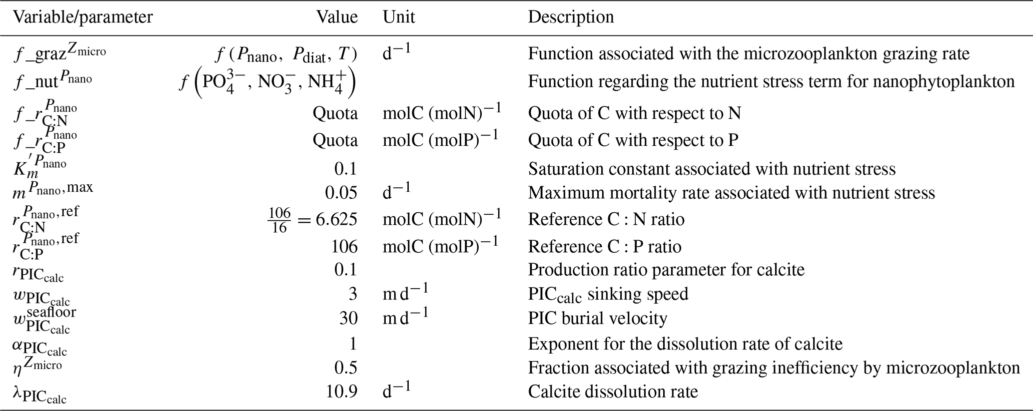
C5 PISCESv1

• Reference used: Aumont (2005)

• Marine biogeochemical model of CNRM-ESM1 (CMIP5), IPSL-CM5A-LR (CMIP5), IPSL-CM5A-MR (CMIP5), and IPSL-CM5B-LR (CMIP5)

•  

  PIC balance:

•  

  $\frac{{\mathrm{DPIC}}_{\mathrm{calc}}^v}{\mathrm{D}t}=\mathrm{Pr}\left({\mathrm{PIC}}_{\mathrm{calc}}^v\right)-\mathrm{Di}\left({\mathrm{PIC}}_{\mathrm{calc}}^v\right)-w_{{\mathrm{PIC}}_{\mathrm{calc}}}\cdot \frac{\partial {\mathrm{PIC}}_{\mathrm{calc}}^v}{\partial z}$

•  

  PIC export at 100 m:

•  

  Ex$\left({\mathrm{PIC}}_{\mathrm{calc}}\right)\left(\mathrm{100}\right)=w_{{\mathrm{PIC}}_{\mathrm{calc}}}\left(\mathrm{100}\right)\cdot {\mathrm{PIC}}_{\mathrm{calc}}\left(\mathrm{100}\right)$

•  

  PIC production:

•  

  $\mathrm{Pr}\left({\mathrm{PIC}}_{\mathrm{calc}}^v\right)=\mathrm{PREREQ}\cdot [{\mathit{\eta }}^Z\cdot (f\mathit{\_}{\mathrm{graz}}^{Z_{\mathrm{micro}}}\cdot Z_{\mathrm{micro}}^v$

•  

  $+f\mathit{\_}{\mathrm{graz}}^{Z_{\mathrm{meso}}}\cdot Z_{\mathrm{meso}}^v)+m^{P_{\mathrm{nano}}}\cdot \frac{P_{\mathrm{nano}}^v}{K_m^{P_{\mathrm{nano}}}+P_{\mathrm{nano}}^v}\cdot P_{\mathrm{nano}}$

•  

  $+{\mathit{\mu }}^{P_{\mathrm{nano}}}\cdot {\left(P_{\mathrm{nano}}^v\right)}^{\mathrm{2}}]$

•  

  $\mathrm{PREREQ}=r_{{\mathrm{PIC}}_{\mathrm{calc}}}\cdot f\mathit{\_}{\mathrm{nut}}^{P_{\mathrm{nano}}}$

•  

  $\cdot max\left(\mathrm{0.0001},\frac{T}{\mathrm{2}+T}\right)\cdot max\left(\mathrm{1},\frac{P_{\mathrm{nano}}^v}{\mathrm{2}}\right)$

•  

  PIC sinking speed:

•  

  $w_{{\mathrm{PIC}}_{\mathrm{calc}}}=w_{{\mathrm{POC}}_{\mathrm{large}}}=w_{{\mathrm{POC}}_{\mathrm{large}}}^{\min }+\left(w_{{\mathrm{POC}}_{\mathrm{large}}}^{\mathrm{ref}}-w_{{\mathrm{POC}}_{\mathrm{large}}}^{\min }\right)$

•  

  $\cdot \frac{max\left(\mathrm{0},z-z_{\mathrm{mld}}\right)}{z_{\mathrm{ref}}}$

Table C5 PISCESv1 parameters.

•  

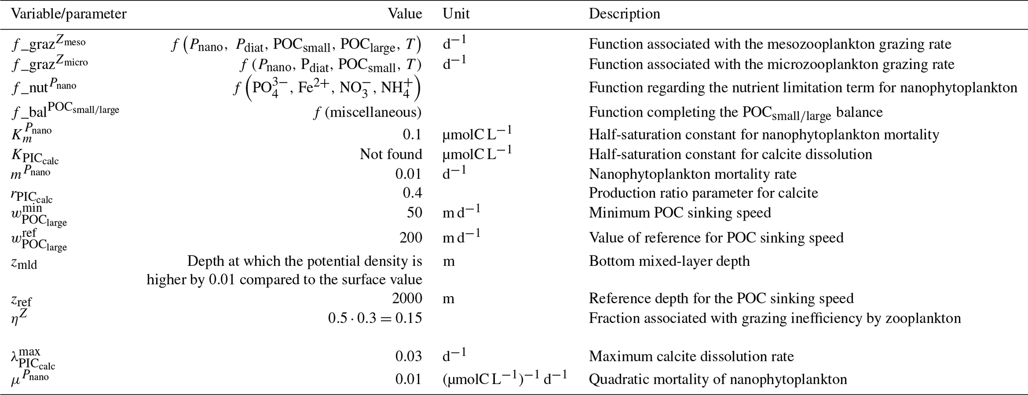
  PIC dissolution:

•  

  $\mathrm{Di}\left({\mathrm{PIC}}_{\mathrm{calc}}^v\right)={\mathit{\lambda }}_{{\mathrm{PIC}}_{\mathrm{calc}}}^{\max }\cdot \frac{max\left(\mathrm{0},{\left[{\mathrm{CO}}_{\mathrm{3}}^{\mathrm{2}-}\right]}_{\mathrm{sat}}^{\mathrm{calc}}-\left[{\mathrm{CO}}_{\mathrm{3}}^{\mathrm{2}-}\right]\right)}{K_{{\mathrm{PIC}}_{\mathrm{calc}}}+{\left[{\mathrm{CO}}_{\mathrm{3}}^{\mathrm{2}-}\right]}_{\mathrm{sat}}^{\mathrm{calc}}-\left[{\mathrm{CO}}_{\mathrm{3}}^{\mathrm{2}-}\right]}\cdot {\mathrm{PIC}}_{\mathrm{calc}}^v$

•  

  Ballast:

•  

  $\frac{\partial {\mathrm{POC}}_{\mathrm{small}}^v}{\partial t}=\left(\mathrm{1}-\mathrm{0.5}\cdot R_{{\mathrm{PIC}}_{\mathrm{calc}}}\right)$

•  

  $\cdot \left(m^{P_{\mathrm{nano}}}\cdot \frac{P_{\mathrm{nano}}^v}{K_m^{P_{\mathrm{nano}}}+P_{\mathrm{nano}}^v}\cdot P_{\mathrm{nano}}^v+{\mathit{\mu }}^{P_{\mathrm{nano}}}\cdot {\left(P_{\mathrm{nano}}^v\right)}^{\mathrm{2}}\right)$

•  

  $+f\mathit{\_}{\mathrm{bal}}^{{\mathrm{POC}}_{\mathrm{small}}}$

•  

  $\frac{\partial {\mathrm{POC}}_{\mathrm{large}}^v}{\partial t}=\mathrm{0.5}\cdot R_{{\mathrm{PIC}}_{\mathrm{calc}}}$

•  

  $\cdot \left(m^{P_{\mathrm{nano}}}\cdot \frac{P_{\mathrm{nano}}^v}{K_m^{P_{\mathrm{nano}}}+P_{\mathrm{nano}}^v}\cdot P_{\mathrm{nano}}^v+{\mathit{\mu }}^{P_{\mathrm{nano}}}\cdot (P_{\mathrm{nano}}^v{)}^{\mathrm{2}}\right)$

•  

  $+f\mathit{\_}{\mathrm{bal}}^{{\mathrm{POC}}_{\mathrm{large}}}$

•  

  Protection effect: N/A

•  

  PIC burial: N/A

C6 PISCESv2 and PISCESv2-gas

• Reference used: Aumont et al. (2015)

• Marine biogeochemical model of CNRM-ESM2-1 (CMIP6) and IPSL-CM6A-LR (CMIP6)

•  

  PIC balance:

•  

  $\frac{{\mathrm{DPIC}}_{\mathrm{calc}}^v}{\mathrm{D}t}=\mathrm{Pr}\left({\mathrm{PIC}}_{\mathrm{calc}}^v\right)-\mathrm{Di}\left({\mathrm{PIC}}_{\mathrm{calc}}^v\right)-w_{{\mathrm{PIC}}_{\mathrm{calc}}}\cdot \frac{\partial {\mathrm{PIC}}_{\mathrm{calc}}^v}{\partial z}$

•  

  PIC export at 100 m:

•  

  Ex$\left({\mathrm{PIC}}_{\mathrm{calc}}\right)\left(\mathrm{100}\right)=w_{{\mathrm{PIC}}_{\mathrm{calc}}}\left(\mathrm{100}\right)\cdot {\mathrm{PIC}}_{\mathrm{calc}}^v\left(\mathrm{100}\right)$

•  

  Production:

•  

  $\mathrm{Pr}\left({\mathrm{PIC}}_{\mathrm{calc}}^v\right)=\mathrm{PREREQ}\cdot [{\mathit{\eta }}^{Z_{\mathrm{micro}}}\cdot f\mathit{\_}{\mathrm{graz}}^{Z_{\mathrm{micro}}}\cdot Z_{\mathrm{micro}}^v$

•  

  $+{\mathit{\eta }}^{Z_{\mathrm{meso}}}\cdot f\mathit{\_}{\mathrm{graz}}^{Z_{\mathrm{meso}}}\cdot Z_{\mathrm{meso}}^v$

•  

  $+m^{P_{\mathrm{nano}}}\cdot \frac{P_{\mathrm{nano}}^v}{K_m^{P_{\mathrm{nano}}}+P_{\mathrm{nano}}^v}\cdot P_{\mathrm{nano}}^v$

•  

  $+\mathrm{sh}\cdot {\mathit{\mu }}^{{}^{\prime }{P}_{\mathrm{nano}}}\cdot {\left(P_{\mathrm{nano}}^v\right)}^{\mathrm{2}}]$

•  

  $\mathrm{PREREQ}=r_{{\mathrm{PIC}}_{\mathrm{calc}}}\cdot f\mathit{\_}{\mathrm{nut}}^{P_{\mathrm{nano}}}\cdot \frac{T}{\mathrm{0.1}+T}\cdot max\left(\mathrm{1},\frac{P_{\mathrm{nano}}^v}{\mathrm{2}}\right)$

•  

  $\cdot \frac{max\left(\mathrm{0},\mathrm{PAR}-\mathrm{1}\right)}{\mathrm{4}+\mathrm{PAR}}\cdot \frac{\mathrm{30}}{\mathrm{30}+\mathrm{PAR}}\cdot \left[\mathrm{1}+\exp \left(\frac{-{\left(T-\mathrm{10}\right)}^{\mathrm{2}}}{\mathrm{25}}\right)\right]$

•  

  $\cdot min\left(\mathrm{1},\frac{\mathrm{50}}{z_{\mathrm{mld}}}\right)$

•  

  PIC sinking speed:

•  

  $w_{{\mathrm{PIC}}_{\mathrm{calc}}}=w_{{\mathrm{POC}}_{\mathrm{large}}}=w_{{\mathrm{POC}}_{\mathrm{large}}}^{\min }+\left(w_{{\mathrm{POC}}_{\mathrm{large}}}^{\mathrm{ref}}-w_{{\mathrm{POC}}_{\mathrm{large}}}^{\min }\right)$

•  

  $\cdot \frac{max\left(\mathrm{0},z-max\left(z_{\mathrm{eld}},z_{\mathrm{mld}}\right)\right)}{z_{\mathrm{ref}}}$

Table C6 PISCESv2 and PISCESv2-gas parameters.

•  

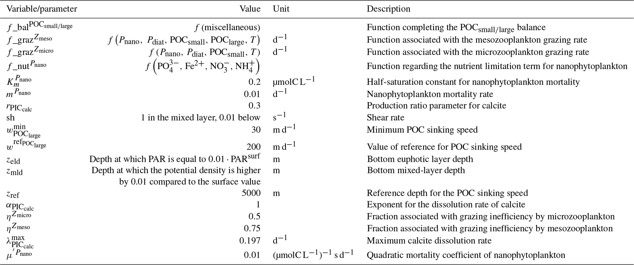
  PIC dissolution:

•  

  $\mathrm{Di}\left({\mathrm{PIC}}_{\mathrm{calc}}^v\right)={\mathit{\lambda }}_{{\mathrm{PIC}}_{\mathrm{calc}}}^{\max }\cdot {\left(max\left(\mathrm{0},\mathrm{1}-\frac{\left[{\mathrm{CO}}_{\mathrm{3}}^{\mathrm{2}-}\right]}{{\left[{\mathrm{CO}}_{\mathrm{3}}^{\mathrm{2}-}\right]}_{\mathrm{sat}}^{\mathrm{calc}}}\right)\right)}^{{\mathit{\alpha }}_{{\mathrm{PIC}}_{\mathrm{calc}}}}$

•  

  $\cdot {\mathrm{PIC}}_{\mathrm{calc}}^v$

•  

  Ballast effect:

•  

  $\frac{\partial {\mathrm{POC}}_{\mathrm{small}}^v}{\partial t}=\left(\mathrm{1}-\mathrm{0.5}\cdot R_{{\mathrm{PIC}}_{\mathrm{calc}}}\right)$

•  

  $\cdot \left(m^{P_{\mathrm{nano}}}\cdot \frac{P_{\mathrm{nano}}^v}{K_m^{P_{\mathrm{nano}}}+P_{\mathrm{nano}}^v}\cdot P_{\mathrm{nano}}+\mathrm{sh}\cdot {\mathit{\mu }}^{{}^{\prime }{P}_{\mathrm{nano}}}\cdot {\left(P_{\mathrm{nano}}^v\right)}^{\mathrm{2}}\right)$

•  

  $+f\mathit{\_}{\mathrm{bal}}^{{\mathrm{POC}}_{\mathrm{small}}}$

•  

  $\frac{\partial {\mathrm{POC}}_{\mathrm{large}}^v}{\partial t}=\mathrm{0.5}\cdot R_{{\mathrm{PIC}}_{\mathrm{calc}}}\cdot$

•  

  $\left(m^{P_{\mathrm{nano}}}\cdot \frac{P_{\mathrm{nano}}^v}{K_m^{P_{\mathrm{nano}}}+P_{\mathrm{nano}}^v}\cdot P_{\mathrm{nano}}+\mathrm{sh}\cdot {\mathit{\mu }}^{{}^{\prime }{P}_{\mathrm{nano}}}\cdot {\left(P_{\mathrm{nano}}^v\right)}^{\mathrm{2}}\right)$

•  

  $+f\mathit{\_}{\mathrm{bal}}^{{\mathrm{POC}}_{\mathrm{large}}}$

•  

  Protection effect: N/A

•  

  PIC burial:

•  

  $\mathrm{Bu}\left({\mathrm{PIC}}_{\mathrm{calc}}\right)=\mathrm{0.6}\cdot min\left(\mathrm{1},\mathrm{1.3}\cdot \frac{{\mathrm{\Omega }}_{\mathrm{calc}}-\mathrm{0.8}}{{\mathrm{\Omega }}_{\mathrm{calc}}-\mathrm{0.6}}\right)$

•  

    ⋅Ex(PIC_calc)^seafloor

•  

  A bug has been noted and addressed with regards to the burial of PIC in a recent release of the model.

C7 WOMBAT

• References used: Oke et al. (2013), Law et al. (2017), and Ziehn et al. (2020)

• Marine biogeochemical model of ACCESS-ESM1-5 (CMIP6)

•  

  PIC balance:

•  

  $\frac{{\mathrm{DPIC}}^v}{\mathrm{D}t}=\mathrm{Pr}\left({\mathrm{PIC}}^v\right)-\mathrm{Di}\left({\mathrm{PIC}}^v\right)-w_{\mathrm{PIC}}\cdot \frac{\partial {\mathrm{PIC}}^v}{\partial z}$

•  

  PIC export at 100 m:

•  

  Ex$\left({\mathrm{PIC}}_{\mathrm{calc}}\right)\left(\mathrm{100}\right)=w_{\mathrm{PIC}}\cdot {\mathrm{PIC}}^v\left(\mathrm{100}\right)$

•  

  PIC production:

•  

  $\mathrm{Pr}\left({\mathrm{PIC}}^v\right)=r_{\mathrm{PIC}}\cdot r_{\mathrm{C}:\mathrm{N}}\cdot \left[{\mathit{\eta }}^Z\cdot \mathrm{PREREQ}\cdot Z^{v,\mathrm{N}}+{\mathit{\mu }}^Z\cdot {\left(Z^{v,\mathrm{N}}\right)}^{\mathrm{2}}+{\mathit{\mu }}^P\cdot (P^{v,\mathrm{N}}{)}^{\mathrm{2}}\right]$

•  

  $\mathrm{PREREQ}=g^{Z,\max }\cdot \frac{{\mathit{ϵ}}^Z\cdot (P^{v,\mathrm{N}}{)}^{\mathrm{2}}}{g^{Z,\max }+{\mathit{ϵ}}^Z\cdot (P^{v,\mathrm{N}}{)}^{\mathrm{2}}}$

•  

  PIC sinking speed: w_PIC

•  

  PIC dissolution:

•  

  $\mathrm{Di}\left({\mathrm{PIC}}^v\right)={\mathit{\lambda }}_{\mathrm{PIC}}\cdot {\mathrm{PIC}}^v$

•  

  Ballast effect: N/A

•  

  Protection effect: N/A

•  

  PIC burial: N/A

Table C7 WOMBAT parameters.

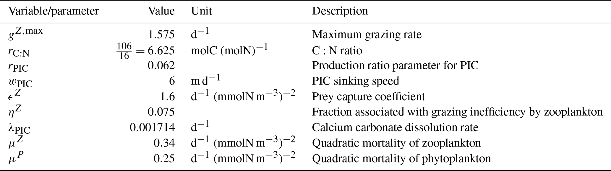
C8 OECO1

• References used: Yoshikawa et al. (2008) and Watanabe et al. (2011)

• Marine biogeochemical model of MIROC-ESM (CMIP5) and MIROC-ESM-CHEM (CMIP5)

•  

  PIC balance:

•  

  $\frac{\mathrm{D}\left({\mathrm{PIC}}^v\right)}{\mathrm{D}t}=\left\{\begin{array}{l}\mathrm{Pr}\left({\mathrm{PIC}}^v\right)-\mathrm{Di}\left({\mathrm{PIC}}^v\right)-w_{\mathrm{PIC}}\cdot \frac{\partial {\mathrm{PIC}}^v}{\partial z}\mathrm{for}z<\mathrm{200}\mathrm{m}\\ \mathrm{Pr}\left({\mathrm{PIC}}^v\right)-\mathrm{Di}\left({\mathrm{PIC}}^v\right)+w_{\mathrm{PIC}}\cdot {\mathrm{PIC}}^v\left(\mathrm{200}\right)\cdot \mathrm{0.858}\cdot \left(\frac{{\mathrm{200}}^{\mathrm{0.858}}}{z^{\mathrm{1.858}}}\right)\mathrm{for}z\ge \mathrm{200}\mathrm{m}\end{array}\right.$

•  

  PIC production:

•  

  $\mathrm{Pr}\left({\mathrm{PIC}}^v\right)=r_{\mathrm{PIC}}\cdot r_{\mathrm{C}:\mathrm{N}}\cdot \left[\frac{g^{Z,\max }\cdot {\mathit{ϵ}}^Z\cdot {\left(P^{v,\mathrm{N}}\right)}^{\mathrm{2}}}{g^{Z,\max }+{\mathit{ϵ}}^Z\cdot {\left(P^{v,\mathrm{N}}\right)}^{\mathrm{2}}}\cdot Z^{v,\mathrm{N}}+\left(f\mathit{\_}{\mathrm{growth}}^P-m^P\right)\cdot P^{v,\mathrm{N}}\right]$

•  

  PIC sinking speed: w_PIC in the top 200 m and N/A

•  

  below 200 m

•  

  PIC dissolution:

•  

  $\mathrm{Di}\left({\mathrm{PIC}}^v\right)={\mathit{\lambda }}_{\mathrm{PIC}}\cdot {\left(\mathrm{1.066}\right)}^T\cdot {\mathrm{PIC}}^v$

•  

  Ballast effect: N/A

•  

  Protection effect: N/A

•  

  PIC burial: N/A

Table C8 OECO1 parameters.

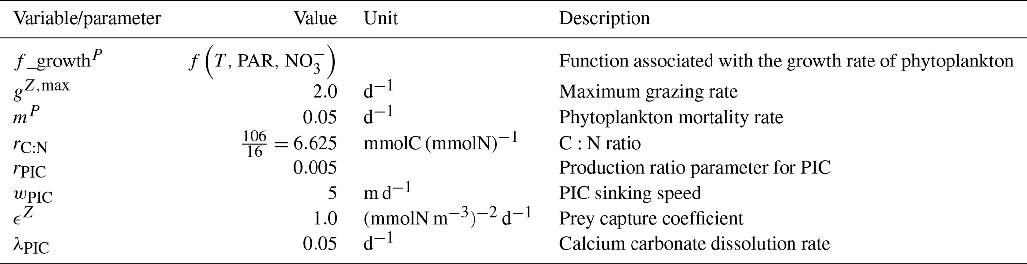
C9 OECO2

• References used: Schmittner et al. (2008) and Hajima et al. (2020)

• Marine biogeochemical model of MIROC-ES2L (CMIP6)

•  

  PIC balance:

•  

  $\frac{\mathrm{D}\left({\mathrm{PIC}}^v\right)}{\mathrm{D}t}=\mathrm{Pr}\left({\mathrm{PIC}}^v\right)-\mathrm{Di}\left({\mathrm{PIC}}^v\right)$

•  

  PIC export at 100 m:

•  

  Ex$\left(\mathrm{PIC}\right)\left(\mathrm{100}\right)={\int }_{z^{\prime }}\mathrm{Pr}\left({\mathrm{PIC}}^v\right)\mathrm{d}z\cdot \exp \left(\frac{-\mathrm{100}}{D_{\mathrm{PIC}}}\right)$

•  

  $={\int }_{z^{\prime }}\mathrm{Pr}\left({\mathrm{PIC}}^v\right)\mathrm{d}{z}^{\prime }-{\int }_{\mathrm{0}}^{\mathrm{100}}\mathrm{Di}\left({\mathrm{PIC}}^v\right)\mathrm{d}{z}^{\prime }$

•  

  PIC production:

•  

  $\mathrm{Pr}\left({\mathrm{PIC}}^v\right)=r_{\mathrm{PIC}}\cdot r_{\mathrm{C}:\mathrm{N}}\cdot [{\mathit{\eta }}^Z\cdot \frac{g^{Z,\max }\cdot {\mathit{ϵ}}^Z\cdot {\left(P_{\text{non-diaz}}^{v,\mathrm{N}}\right)}^{\mathrm{2}}}{g^{Z,\max }+{\mathit{ϵ}}^Z\cdot {\left(P_{\text{non-diaz}}^{v,\mathrm{N}}\right)}^{\mathrm{2}}}\cdot Z^{v,\mathrm{N}}$

•  

  $+{\mathit{\mu }}^{P_{\text{non-diaz}}}\cdot {\left(P_{\text{non-diaz}}^{v,\mathrm{N}}\right)}^{\mathrm{2}}+{\mathit{\mu }}^Z\cdot {\left(Z^{v,\mathrm{N}}\right)}^{\mathrm{2}}]$

•  

  PIC sinking speed: N/A

•  

  PIC dissolution:

•  

  $\mathrm{Di}\left({\mathrm{PIC}}^v\right)\left(z\right)=\frac{\partial \left(\mathrm{Ex}\left(\mathrm{PIC}\right)\right)}{\partial z}\left(z\right)=\frac{\mathrm{1}}{D_{\mathrm{PIC}}}\cdot {\int }_{z^{\prime }}\mathrm{Pr}\left({\mathrm{PIC}}^v\right)\mathrm{d}{z}^{\prime }$

•  

  $\cdot \exp \left(\frac{-z}{D_{\mathrm{PIC}}}\right)$

•  

  Ballast effect: N/A

•  

  Protection effect: N/A

•  

  PIC burial: N/A

Table C9 OECO2 parameters.

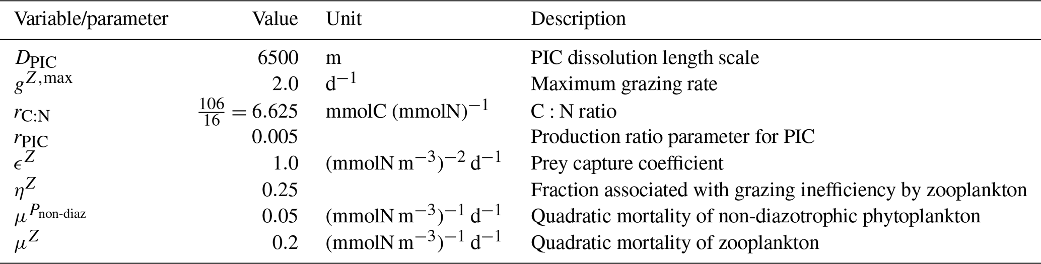
C10 diat-HadOCC

• Reference used: Totterdell (2019)

• Marine biogeochemical model of HadGEM2-CC (CMIP5) and HadGEM2-ES (CMIP5)

•  

  PIC balance:

•  

  $\frac{\partial {\mathrm{PIC}}^v\left(n\right)}{\partial t}=\mathrm{Pr}\left({\mathrm{PIC}}^v\right)\left(n\right)-\mathrm{Di}\left({\mathrm{PIC}}^v\right)\left(n\right)$

•  

  PIC export at 100 m:

•  

  Ex$\left(\mathrm{PIC}\right)\left(\mathrm{100}\right)={\sum }_{m\text{for}z\le \mathrm{100}\mathrm{m}}\mathrm{Pr}\left({\mathrm{PIC}}^v\right)\left(m\right)\cdot h\left(m\right)$

•  

  PIC production:

•  

  $\mathrm{Pr}\left({\mathrm{PIC}}^v\right)\left(n\right)=r_{\mathrm{PIC}}\cdot r_{\mathrm{C}:\mathrm{N}}\cdot \mathrm{Pr}\left(P^{v,\mathrm{N}}\right)\left(n\right)$

•  

  PIC sinking speed: N/A

•  

  PIC dissolution:

•  

  $\mathrm{Di}\left({\mathrm{PIC}}^v\left(n\right)\right)=\left\{\begin{array}{l}\frac{{\sum }_m\mathrm{Pr}\left({\mathrm{PIC}}^v\right)\left(m\right)\cdot h\left(m\right)}{z_{\mathrm{sfd}}-z_{\mathrm{lyd}}}\text{for a layer}n\mathrm{below}\mathrm{the}\mathrm{lysocline}\\ \mathrm{0}\text{for a layer}n\mathrm{above}\mathrm{the}\mathrm{lysocline}\end{array}\right.$

•  

  When z_sfd≤z_lyd, all the PIC is dissolved

•  

  in the bottom level.

•  

  Ballast effect: N/A

•  

  Protection effect: N/A

•  

  PIC burial: N/A

Table C10 Diat-HadOCC parameters.

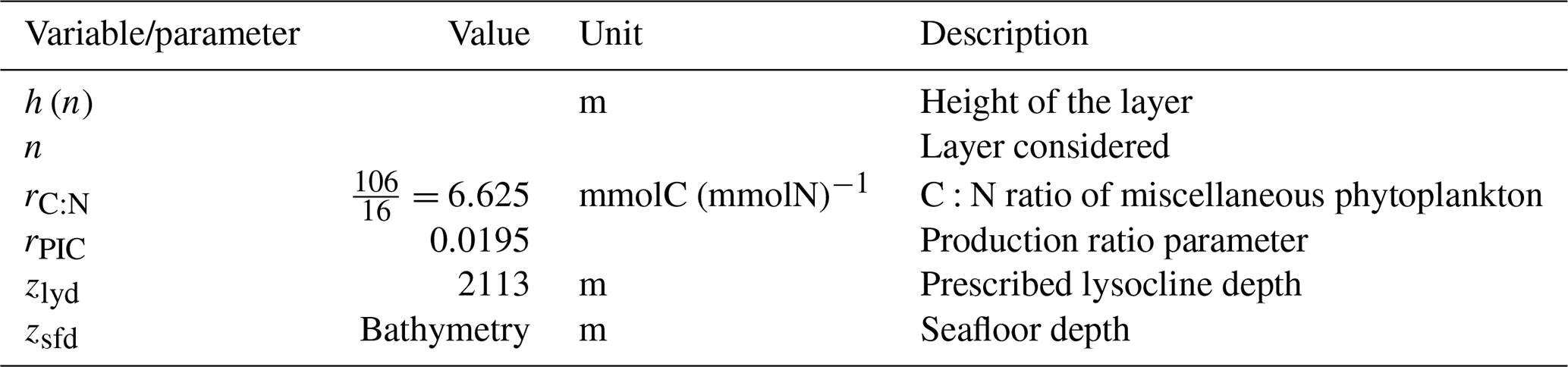
C11 MEDUSA-2.1

• Reference used: Yool et al. (2013b)

• Marine biogeochemical model of UKESM1-0-LL (CMIP6)

•  

  PIC balance:

•  

  Ex$\left({\mathrm{PIC}}_{\mathrm{calc}}\right)(n+\mathrm{1})=\mathrm{Ex}\left({\mathrm{PIC}}_{\mathrm{calc}}\right)\left(n\right)-$

•  

  $\mathrm{Di}\left(\mathrm{Ex}\left({\mathrm{PIC}}_{\mathrm{calc}}\right)\right)\left(n\right)\cdot h\left(n\right)+\mathrm{Pr}\left({\mathrm{PIC}}_{\mathrm{calc}}^v\right)\left(n\right)\cdot h\left(n\right)$

•  

  PIC export at 100 m: no specific calculation

•  

  PIC production:

•  

  $\mathrm{Pr}\left({\mathrm{PIC}}_{\mathrm{calc}}^v\right)=r_{{\mathrm{PIC}}_{\mathrm{calc}}}$

•  

  $\cdot \left[\right(r_{\mathrm{C}:\mathrm{N}}^{P_{\mathrm{diat}}}\cdot {\mathit{\eta }}^{P_{\mathrm{diat}}}\cdot m^{P_{\mathrm{diat}},\max }\cdot \frac{P_{\mathrm{diat}}}{K_m^{P_{\mathrm{diat}}}+P_{\mathrm{diat}}}\cdot P_{\mathrm{diat}}^v)$

•  

  $+\left(r_{\mathrm{C}:\mathrm{N}}^{Z_{\mathrm{meso}}}\cdot {\mathit{\eta }}^{Z_{\mathrm{meso}}}\cdot m^{Z_{\mathrm{meso}},\max }\cdot \frac{Z_{\mathrm{meso}}}{K_m^{Z_{\mathrm{meso}}}+Z_{\mathrm{meso}}}\cdot Z_{\mathrm{meso}}^v\right)]$

•  

  $\cdot {\left[max\left(\mathrm{0},{\mathrm{\Omega }}_{\mathrm{calcite}}-\mathrm{1}\right)\right]}^{{\mathit{\beta }}_{{\mathrm{PIC}}_{\mathrm{calc}}}}$

•  

  PIC sinking speed: N/A

•  

  PIC dissolution:

•  

  $\mathrm{Di}\left(\mathrm{Ex}\left({\mathrm{PIC}}_{\mathrm{calc}}\left(n\right)\right)\right)=\left\{\begin{array}{l}\mathrm{Ex}\left({\mathrm{PIC}}_{\mathrm{calc}}\left(n\right)\right)\cdot \frac{\mathrm{1}-\exp \left(-\frac{h\left(n\right)}{D_{{\mathrm{PIC}}_{\mathrm{calc}}}}\right)}{h\left(n\right)}\text{for a layer}n\mathrm{below}\mathrm{the}\mathrm{lysocline}\\ \mathrm{0}\text{for a layer}n\mathrm{above}\mathrm{the}\mathrm{lysocline}\end{array}\right.$

Table C11 MEDUSA-2.1 parameters.

•  

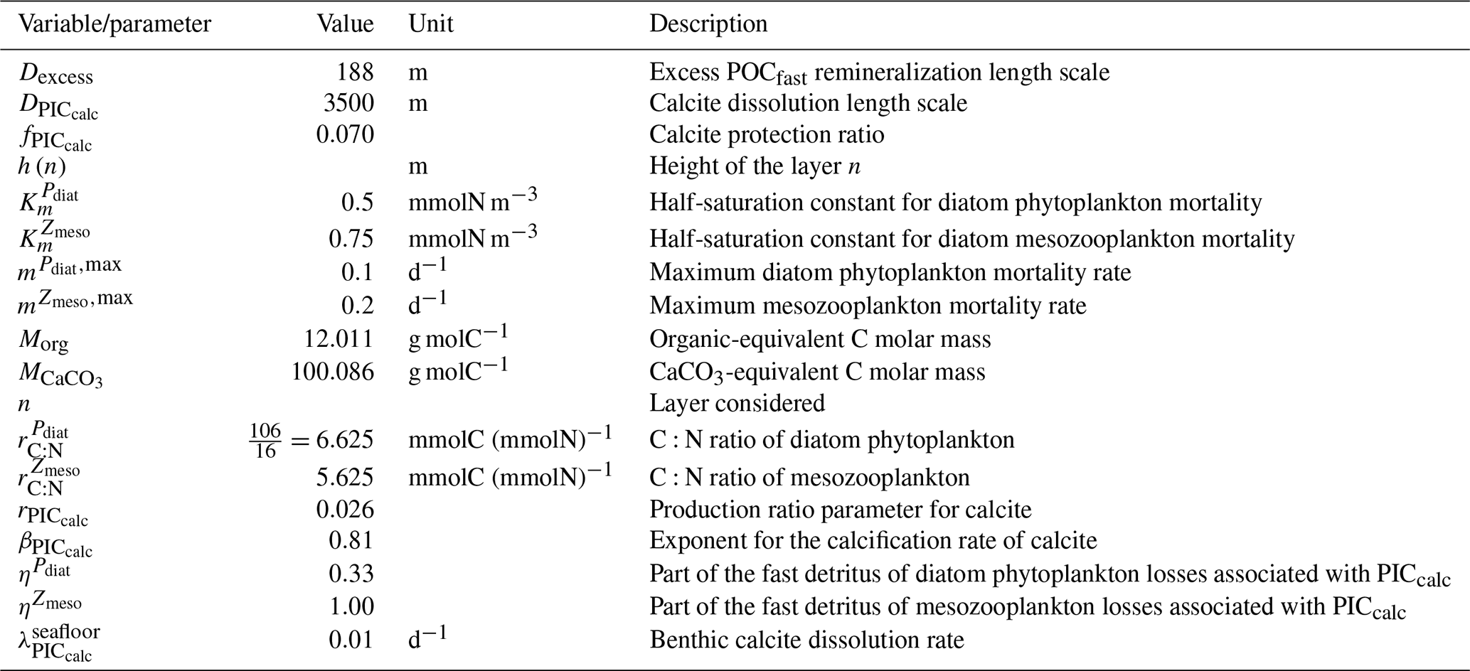
  Ballast effect: N/A

•  

  Protection effect:

•  

  Ex$\left({\mathrm{POC}}_{\mathrm{fast}}\right)(n+\mathrm{1})=\mathrm{Ex}\left({\mathrm{POC}}_{\mathrm{fast}}^{\mathrm{protected}}\right)\left(n\right)$

•  

  $+\left(\mathrm{Ex}\left({\mathrm{POC}}_{\mathrm{fast}}\right)\left(n\right)-\mathrm{Ex}\left({\mathrm{POC}}_{\mathrm{fast}}^{\mathrm{protected}}\right)\left(n\right)\right)$

•  

  $\cdot \exp \left(-\frac{h\left(n\right)}{D_{\mathrm{excess}}}\right)$

•  

  Ex$\left({\mathrm{POC}}_{\mathrm{fast}}^{\mathrm{protected}}\right)\left(n\right)=\mathrm{Ex}\left({\mathrm{POC}}_{\mathrm{fast}}^{\mathrm{protected},{\mathrm{PIC}}_{\mathrm{calc}}}\right)\left(n\right)$

•  

  $+\mathrm{Ex}\left({\mathrm{POC}}_{\mathrm{fast}}^{\mathrm{protected},\mathrm{PISi}}\right)\left(n\right)$

•  

  Ex$\left({\mathrm{POC}}_{\mathrm{fast}}^{\mathrm{protected},{\mathrm{PIC}}_{\mathrm{calc}}}\right)\left(n\right)=f_{{\mathrm{PIC}}_{\mathrm{calc}}}\cdot \frac{M_{{\mathrm{CaCO}}_{\mathrm{3}}}}{M_{\mathrm{org}}}$

•  

    ⋅Ex(PIC_calc)(n)

•  

  PIC temporary storage at the seafloor (no burial):

•  

  $\mathrm{St}\left({\mathrm{PIC}}_{\mathrm{calc}}\right)=\mathrm{Ex}{\left({\mathrm{PIC}}_{\mathrm{calc}}\right)}^{\mathrm{seafloor}}-{\mathit{\lambda }}_{{\mathrm{PIC}}_{\mathrm{calc}}}^{\mathrm{seafloor}}\cdot {\left({\mathrm{PIC}}_{\mathrm{calc}}^s\right)}^{\mathrm{seafloor}}$

C12 HAMOCC5.2 and HAMOCC6

• Reference used: Ilyina et al. (2013)

• Marine biogeochemical model of MPI-ESM-LR (CMIP5), MPI-ESM-MR (CMIP5), MPI-ESM1-2-LR (CMIP6), and MPI-ESM1-2-HR (CMIP6)

•  

  PIC balance:

•  

  $\frac{\partial {\mathrm{PIC}}_{\mathrm{calc}}^v}{\partial t}=\mathrm{Pr}\left({\mathrm{PIC}}_{\mathrm{calc}}^v\right)-\mathrm{Di}\left({\mathrm{PIC}}_{\mathrm{calc}}^v\right)-w_{{\mathrm{PIC}}_{\mathrm{calc}}}\cdot \frac{\partial {\mathrm{PIC}}_{\mathrm{calc}}^v}{\partial z}$

•  

  PIC export at 100 m:

•  

  Ex$\left({\mathrm{PIC}}_{\mathrm{calc}}\right)=w_{{\mathrm{PIC}}_{\mathrm{calc}}}\cdot {\mathrm{PIC}}_{\mathrm{calc}}^v\left(\mathrm{100}\right)$

•  

  PIC production:

•  

  $\mathrm{Pr}\left({\mathrm{PIC}}_{\mathrm{calc}}^v\right)=r_{{\mathrm{PIC}}_{\mathrm{calc}}}\cdot r_{\mathrm{C}:\mathrm{P}}\cdot \frac{K_{\mathrm{Si}(\mathrm{OH}{)}_{\mathrm{4}}}}{K_{\mathrm{Si}(\mathrm{OH}{)}_{\mathrm{4}}}+\left[\mathrm{Si}(\mathrm{OH}{)}_{\mathrm{4}}\right]}$

•  

  $\cdot \left[m^{\mathrm{P}}\cdot \left(P^{v,\mathrm{P}}-P^{v,\mathrm{P},\min }\right)+{\mathit{\eta }}^Z\cdot g^Z\cdot \frac{P^{v,\mathrm{P}}-P^{v,\mathrm{P},\min }}{K_Z+P^{v,\mathrm{P},min}}\cdot Z^v+{\mathit{\eta }}^{{}^{\prime }Z}\cdot {\mathit{\mu }}^Z\cdot (Z^{v,\mathrm{P}}-Z^{v,\mathrm{P},\min }{)}^{\mathrm{2}}\right]$

•  

  PIC sinking speed: $w_{{\mathrm{PIC}}_{\mathrm{calc}}}$

•  

  PIC dissolution:

•  

  $\mathrm{Di}\left({\mathrm{PIC}}_{\mathrm{calc}}^v\right)={\mathit{\lambda }}_{{\mathrm{PIC}}_{\mathrm{calc}}}\cdot max\left(\mathrm{0},\frac{K_{\mathrm{sp},\mathrm{calc}}}{\left[{\mathrm{Ca}}^{\mathrm{2}+}\right]}-\left[{\mathrm{CO}}_{\mathrm{3}}^{\mathrm{2}-}\right]\right)\cdot {\mathrm{PIC}}_{\mathrm{calc}}^v$

•  

  Ballast effect: N/A

•  

  Protection effect: N/A

•  

  PIC burial:

•  

  $\mathrm{Bu}\left({\mathrm{PIC}}_{\mathrm{calc}}\right)=f\mathit{\_}{\mathrm{bur}}^{{\mathrm{PIC}}_{\mathrm{calc}}}$

Table C12 HAMOCC5.2 and HAMOCC6 parameters.

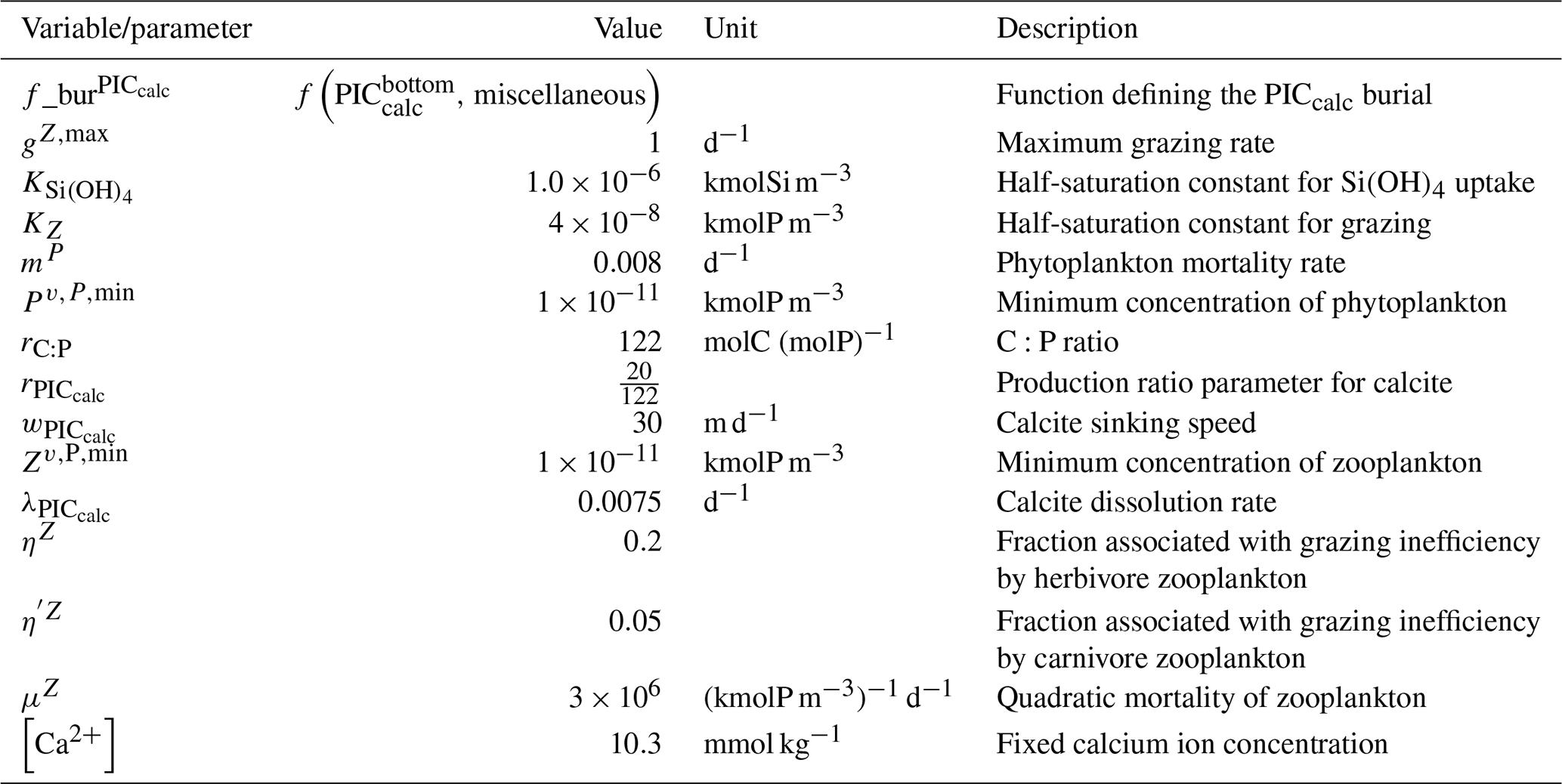
C13 NPZD-MRI

• References used: Schmittner et al. (2008) and Tsujino et al. (2010, 2017)

• Marine biogeochemical model of MRI-ESM1 (CMIP5) and MRI-ESM2-0 (CMIP6)

•  

  PIC balance:

•  

  $\frac{\partial {\mathrm{PIC}}^v}{\partial t}=\mathrm{Pr}\left({\mathrm{PIC}}^v\right)-\mathrm{Di}\left({\mathrm{PIC}}^v\right)$

•  

  PIC export at 100 m:

•  

  Ex$\left({\mathrm{PIC}}_{\mathrm{calc}}\right)\left(\mathrm{100}\right)={\int }_{z^{\prime }}\mathrm{Pr}\left({\mathrm{PIC}}_{\mathrm{calc}}^v\right)\mathrm{d}{z}^{\prime }\cdot \exp \left(\frac{-\mathrm{100}}{D_{{\mathrm{PIC}}_{\mathrm{calc}}}}\right)$

•  

  $={\int }_{z^{\prime }}\mathrm{Pr}\left({\mathrm{PIC}}_{\mathrm{calc}}^v\right)\mathrm{d}{z}^{\prime }-{\int }_{\mathrm{0}}^{\mathrm{100}}\mathrm{Di}\left({\mathrm{PIC}}_{\mathrm{calc}}^v\right)\mathrm{d}{z}^{\prime }$

•  

  PIC production:

•  

  $\mathrm{Pr}\left({\mathrm{PIC}}_{\mathrm{calc}}^v\right)=r_{{\mathrm{PIC}}_{\mathrm{calc}}}\cdot r_{\mathrm{C}:\mathrm{N}}\cdot$

•  

  $[{\mathit{\eta }}^Z\cdot \frac{g^{Z,\max }\cdot {\mathit{ϵ}}^Z\cdot {\left(P^{v,\mathrm{N}}\right)}^{\mathrm{2}}}{g^{Z,\max }+{\mathit{ϵ}}^Z\cdot {\left(P^{v,\mathrm{N}}\right)}^{\mathrm{2}}}\cdot Z^{v,\mathrm{N}}+{\mathit{\mu }}^P\cdot {\left(P^{v,\mathrm{N}}\right)}^{\mathrm{2}}$

•  

  $+{\mathit{\mu }}^Z\cdot {\left(Z^{v,\mathrm{N}}\right)}^{\mathrm{2}}]$

•  

  PIC sinking speed: N/A

•  

  PIC dissolution:

•  

  $\mathrm{Di}\left({\mathrm{PIC}}_{\mathrm{calc}}^v\right)\left(z\right)=-\frac{\partial \left(\mathrm{Ex}\left({\mathrm{PIC}}_{\mathrm{calc}}^v\right)\right)}{\partial z}\left(z\right)=\frac{\mathrm{1}}{D_{{\mathrm{PIC}}_{\mathrm{calc}}}}$

•  

  $\cdot {\int }_{z^{\prime }}\mathrm{Pr}\left({\mathrm{PIC}}_{\mathrm{calc}}^v\right)\mathrm{d}{z}^{\prime }\cdot \exp \left(\frac{-z}{D_{{\mathrm{PIC}}_{\mathrm{calc}}}}\right)$

•  

  Ballast effect: N/A

•  

  Protection effect: N/A

•  

  PIC burial: N/A

Table C13 NPZD-MRI parameters.

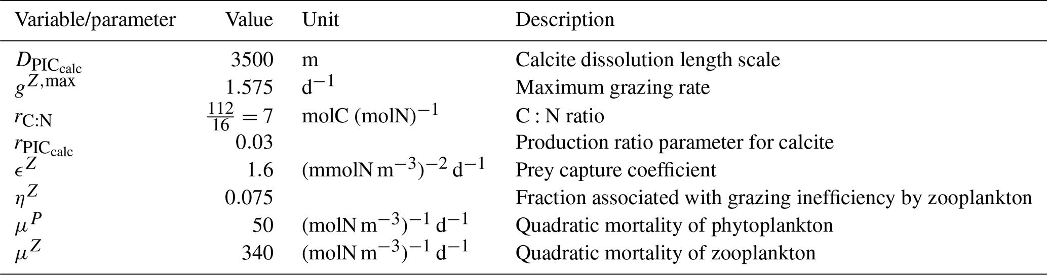
C14 BEC

• References used: Armstrong et al. (2001), Moore et al. (2001, 2004), and a kindly shared document written by Ivan Lima in 2016

• Marine biogeochemical model of CESM1-BGC (CMIP5)

•  

  PIC balance:

•  

  $\frac{\partial {\mathrm{PIC}}_{\mathrm{calc}}^v}{\partial t}=\mathrm{Pr}\left({\mathrm{PIC}}_{\mathrm{calc}}^v\right)-\mathrm{Di}\left({\mathrm{PIC}}_{\mathrm{calc}}^v\right)$

•  

  PIC export at 100 m:

•  

  Ex$\left({\mathrm{PIC}}_{\mathrm{calc}}\right)\left(\mathrm{100}\right)={\int }_{z^{\prime }}\mathrm{Pr}\left({\mathrm{PIC}}_{\mathrm{calc}}^v\right)\mathrm{d}{z}^{\prime }$

•  

  $-{\int }_{\mathrm{0}}^{\mathrm{100}}\mathrm{Di}\left({\mathrm{PIC}}_{\mathrm{calc}}^v\right)\mathrm{d}{z}^{\prime }$

•  

  PIC production:

•  

  $\mathrm{Pr}\left({\mathrm{PIC}}_{\mathrm{calc}}^v\right)=\frac{P_{\mathrm{calc}}^v}{P_{\mathrm{small}}^v}\cdot ({\mathit{\eta }}^Z\cdot g^{P_{\mathrm{small}},\max }\cdot \mathrm{2}\cdot \exp \left(\frac{T-\mathrm{30}}{\mathrm{10}}\right)$

•  

  $\cdot \frac{{\left(P_{\mathrm{small}}^v\right)}^{\mathrm{2}}}{{\left(P_{\mathrm{small}}^v\right)}^{\mathrm{2}}+K_{\mathrm{g}}^{{}^{\prime }{P}_{\mathrm{small}}}}\cdot Z^v+m^{P_{\mathrm{small}}}\cdot P_{\mathrm{small}}^v$

•  

  $+\min \left[b^{P_{\mathrm{small}},\max }\cdot P_{\mathrm{small}}^v,{\mathit{\mu }}^{P_{\mathrm{small}}}\cdot {\left(P_{\mathrm{small}}^v\right)}^{\mathrm{2}}\right])$

•  

  Calcite pool in the phytoplankton group:

•  

  $\mathrm{Pr}\left({\mathrm{PIC}}_{\mathrm{calc}}^v\right)=\left\{\begin{array}{l}min\left(\mathrm{PREREQ}\cdot \frac{P_{\mathrm{small}}^v}{\mathrm{3.0}},\mathrm{0.40}\cdot \mathrm{Pr}\left(P_{\mathrm{small}}^v\right)\right)\\ \mathrm{if}{P}_{\mathrm{small}}^v>\mathrm{3.0}\\ \mathrm{PREREQ}\mathrm{otherwise}\end{array}\right.$

•  

  $\mathrm{PREREQ}=r_{{\mathrm{PIC}}_{\mathrm{calc}}}^{\prime }\cdot \mathrm{Pr}\left(P_{\mathrm{small}}^v\right)\cdot f\mathit{\_}{\mathrm{nut}}^{P_{\mathrm{small}}}$

•  

  $\cdot \left[\mathrm{1}+\left(\frac{max\left(T+\mathrm{2},\mathrm{0}\right)}{\mathrm{4}}-\mathrm{1}\right)\cdot \frac{max\left(\mathrm{2}-T,\mathrm{1}\right)}{\mathrm{2}-T}\right]$

•  

  PIC sinking speed: N/A

Table C14 BEC parameters.

•  

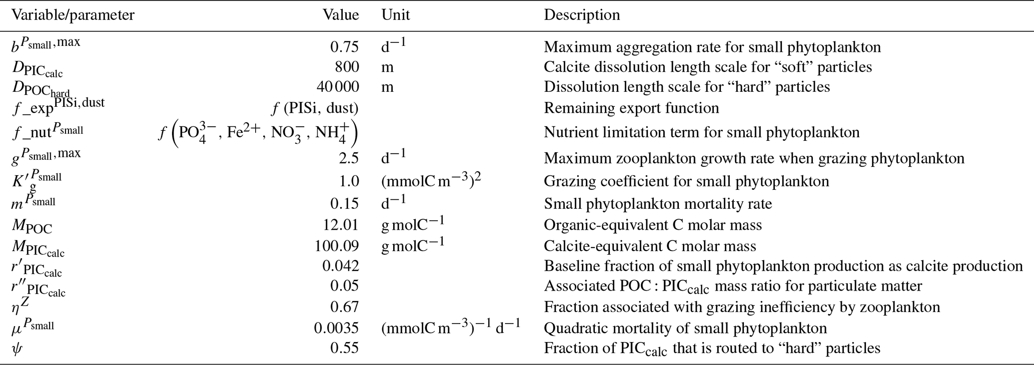
  PIC dissolution:

•  

  $\mathrm{Di}\left({\mathrm{PIC}}_{\mathrm{calc}}\right)\left(z\right)=-\frac{\partial \left(\mathrm{Ex}\left({\mathrm{PIC}}_{\mathrm{calc}}^v\right)\right)}{\partial z}\left(z\right)$

•  

  $={\int }_{z^{\prime }}\mathrm{Pr}\left({\mathrm{PIC}}_{\mathrm{calc}}^v\right)\mathrm{d}{z}^{\prime }\cdot [\left(\mathrm{1}-\mathit{\psi }\right)\cdot \frac{\mathrm{1}}{D_{{\mathrm{PIC}}_{\mathrm{calc}}}}\cdot \exp \left(\frac{-z}{D_{{\mathrm{PIC}}_{\mathrm{calc}}}}\right)$

•  

  $+\mathit{\psi }\cdot \frac{\mathrm{1}}{D_{{\mathrm{POC}}_{\mathrm{hard}}}}\cdot \exp \left(\frac{-z}{D_{{\mathrm{POC}}_{\mathrm{hard}}}}\right)]$

•  

  Ballast effect: N/A

•  

  Protection effect:

•  

  Ex$\left(\mathrm{POC}\right)\left(z\right)=\mathrm{Ex}\left({\mathrm{POC}}^{\mathrm{free}}\right)\left(z\right)+\mathrm{Ex}\left({\mathrm{POC}}^{\mathrm{protected}}\right)\left(z\right)$

•  

  Ex$\left({\mathrm{POC}}^{\mathrm{protected}}\right)\left(z\right)=r{{}^{\prime \prime }}_{{\mathrm{PIC}}_{\mathrm{calc}}}\cdot \frac{M_{{\mathrm{PIC}}_{\mathrm{calc}}}}{M_{\mathrm{POC}}}$

•  

  $\cdot \mathrm{Ex}\left({\mathrm{POC}}^{\mathrm{protected},{\mathrm{PIC}}_{\mathrm{calc}}}\right)\left(z\right)+f\mathit{\_}{\exp }^{\mathrm{PISi},\mathrm{dust}}$

•  

  Ex$\left({\mathrm{POC}}^{\mathrm{protected},{\mathrm{PIC}}_{\mathrm{calc}}}\right)\left(z\right)$

•  

  $=\mathrm{Ex}\left({\mathrm{POC}}_{\mathrm{soft}}^{\mathrm{protected},{\mathrm{PIC}}_{\mathrm{calc}}}\right)\left(z\right)$

•  

  $+\mathrm{Ex}\left({\mathrm{POC}}_{\mathrm{hard}}^{\mathrm{protected},{\mathrm{PIC}}_{\mathrm{calc}}}\right)\left(z\right)$

•  

  Ex$\left({\mathrm{POC}}_{\mathrm{soft}}^{\mathrm{protected},{\mathrm{PIC}}_{\mathrm{calc}}}\right)\left(z\right)=\left(\mathrm{1}-\mathit{\psi }\right)\cdot {\int }_{z^{\prime }}\mathrm{Pr}\left({\mathrm{PIC}}_{\mathrm{calc}}^v\right)\mathrm{d}{z}^{\prime }$

•  

  $\cdot \exp \left(\frac{-z}{D_{{\mathrm{PIC}}_{\mathrm{calc}}}}\right)$

•  

  Ex$\left({\mathrm{POC}}_{\mathrm{hard}}^{\mathrm{protected},{\mathrm{PIC}}_{\mathrm{calc}}}\right)\left(z\right)=\mathit{\psi }\cdot {\int }_{z^{\prime }}\mathrm{Pr}\left({\mathrm{PIC}}_{\mathrm{calc}}^v\right)\mathrm{d}{z}^{\prime }$

•  

  $\cdot \exp \left(\frac{-z}{D_{{\mathrm{POC}}_{\mathrm{hard}}}}\right)$

•  

  PIC burial: N/A

C15 MARBL

• Reference used: Long et al. (2021)

• Marine biogeochemical model of CESM2 (CMIP6),

• CESM2-WACCM-FV2 (CMIP6), CESM2-FV2 (CMIP6),

• and CESM2-WACCM (CMIP6).

•  

  PIC balance:

•  

  $\frac{\partial {\mathrm{PIC}}_{\mathrm{calc}}^v}{\partial t}=\mathrm{Pr}\left({\mathrm{PIC}}_{\mathrm{calc}}^v\right)-\mathrm{Di}\left({\mathrm{PIC}}_{\mathrm{calc}}^v\right)$

•  

  PIC export at 100 m:

•  

  Ex$\left({\mathrm{PIC}}_{\mathrm{calc}}\right)\left(\mathrm{100}\right)={\int }_{z^{\prime }}\mathrm{Pr}\left({\mathrm{PIC}}_{\mathrm{calc}}^v\right)\mathrm{d}{z}^{\prime }$

•  

  $-{\int }_{\mathrm{0}}^{\mathrm{100}}\mathrm{Di}\left({\mathrm{PIC}}_{\mathrm{calc}}^v\right)\mathrm{d}{z}^{\prime }$

•  

  PIC production:

•  

  $\mathrm{Pr}\left({\mathrm{PIC}}_{\mathrm{calc}}^v\right)=\frac{P_{\mathrm{calc}}^v}{P_{\mathrm{small}}^v}\cdot ({\mathit{\eta }}^Z\cdot g^{P_{\mathrm{small}},\max }\cdot \mathrm{2}\cdot \exp \left(\frac{T-\mathrm{30}}{\mathrm{10}}\right)$

•  

  $\cdot \frac{\left(P_{\mathrm{small}}^v\right)}{\left(P_{\mathrm{small}}^v\right)+K_{\mathrm{g}}^{P_{\mathrm{small}}}}\cdot Z^v+m^{P_{\mathrm{small}}}\cdot P_{\mathrm{small}}^v$

•  

  $+min\left[b^{P_{\mathrm{small}},max}\cdot P_{\mathrm{small}}^v,{\mathit{\mu }}^{P_{\mathrm{small}}}\cdot {\left(P_{\mathrm{small}}^v\right)}^{\mathrm{2}}\right])$

•  

  Calcite pool in the phytoplankton group:

•  

  $\mathrm{Pr}\left({\mathrm{PIC}}_{\mathrm{calc}}^v\right)=\left\{\begin{array}{l}min\left(\mathrm{PREREQ}\cdot \frac{P_{\mathrm{small}}^v}{\mathrm{2.5}},\mathrm{0.40}\cdot \mathrm{Pr}\left(P_{\mathrm{small}}^v\right)\right)\\ \mathrm{if}{P}_{\mathrm{small}}^{\mathrm{v}}>\mathrm{2.5}\\ \mathrm{PREREQ}\mathrm{otherwise}\end{array}\right.$

•  

  $\mathrm{PREREQ}=r{{}^{\prime }}_{{\mathrm{PIC}}_{\mathrm{calc}}}$

•  

  $\cdot P\mathrm{r}\left(P_{\mathrm{small}}^v\right)\cdot {\left(f\mathit{\_}{\mathrm{nut}}^{P_{\mathrm{small}}}\right)}^{\mathrm{2}}$

•  

  $\cdot \left[\mathrm{1}+\left(\frac{\max \left(T+\mathrm{2},\mathrm{0}\right)}{\mathrm{6}}-\mathrm{1}\right)\cdot \frac{\max \left(\mathrm{4}-T,\mathrm{1}\right)}{\mathrm{4}-T}\right]$

Table C15 MARBL parameters.

•  

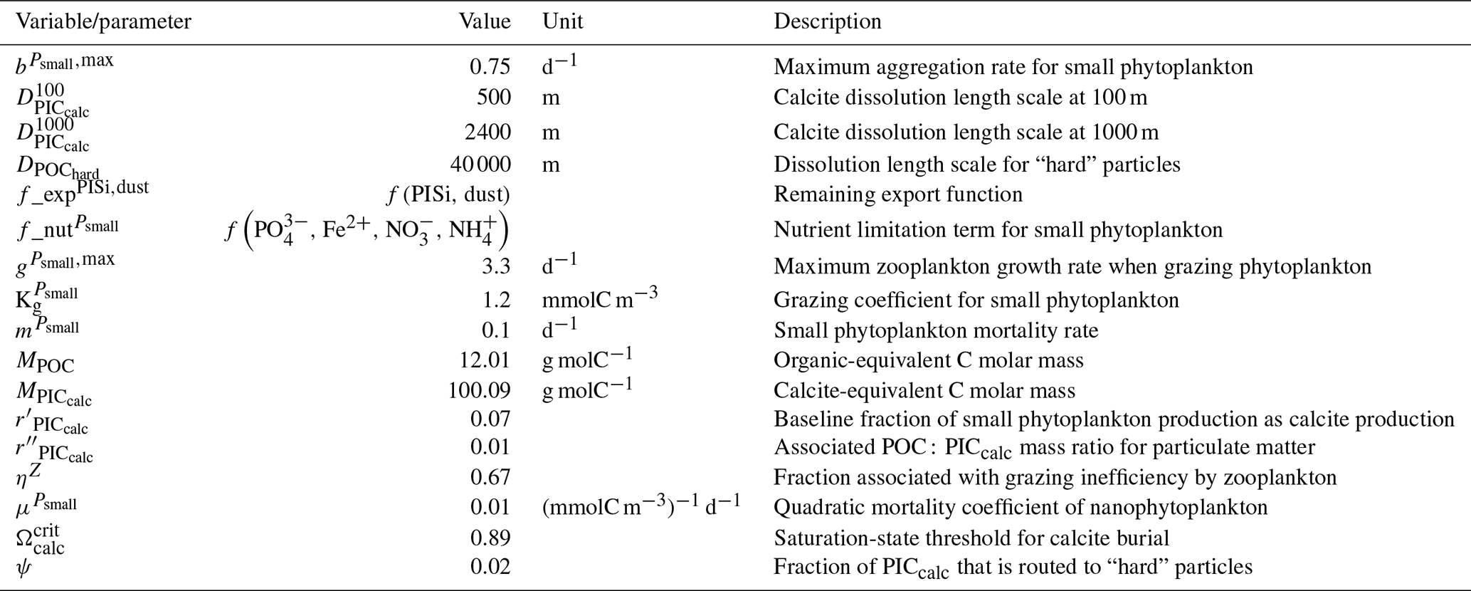
  PIC sinking speed: N/A

•  

  PIC dissolution:

•  

  $\mathrm{Di}\left({\mathrm{PIC}}_{\mathrm{calc}}^v\right)=\frac{\mathrm{1}}{f\mathit{\_}{\mathrm{dist}}^{{\mathrm{PIC}}_{\mathrm{calc}}}}\cdot {\int }_{z^{\prime }}\mathrm{Pr}\left({\mathrm{PIC}}_{\mathrm{calc}}^v\right)\mathrm{d}{z}^{\prime }$

•  

  $\cdot \exp \left(\frac{-z}{f\mathit{\_}{\mathrm{dist}}^{{\mathrm{PIC}}_{\mathrm{calc}}}}\right)$

•  

  $f\mathit{\_}{\mathrm{dist}}^{{\mathrm{PIC}}_{\mathrm{calc}}}=\left\{\begin{array}{l}{D}_{{\mathrm{PIC}}_{\mathrm{calc}}}^{\mathrm{100}}\mathrm{if}z\le \mathrm{100}\\ D_{{\mathrm{PIC}}_{\mathrm{calc}}}^{\mathrm{1000}}\mathrm{if}z\ge \mathrm{1000}\\ D_{{\mathrm{PIC}}_{\mathrm{calc}}}^{\mathrm{prev}}+\frac{D_{{\mathrm{PIC}}_{\mathrm{calc}}}^{\mathrm{next}}-D_{{\mathrm{PIC}}_{\mathrm{calc}}}^{\mathrm{prev}}}{z^{\mathrm{next}}-z^{\mathrm{prev}}}\cdot \left(z-z^{\mathrm{prev}}\right)\mathrm{otherwise}\end{array}\right.$

•  

  Ballast effect: N/A

•  

  Protection effect:

•  

  Ex$\left(\mathrm{POC}\right)\left(z\right)=\mathrm{Ex}\left({\mathrm{POC}}^{\mathrm{free}}\right)\left(z\right)+\mathrm{Ex}\left({\mathrm{POC}}^{\mathrm{protected}}\right)\left(z\right)$

•  

  Ex$\left({\mathrm{POC}}^{\mathrm{protected}}\right)\left(z\right)=r{{}^{\prime \prime }}_{{\mathrm{PIC}}_{\mathrm{calc}}}\cdot \frac{M_{{\mathrm{PIC}}_{\mathrm{calc}}}}{M_{\mathrm{POC}}}$

•  

  $\cdot \mathrm{Ex}\left({\mathrm{POC}}^{\mathrm{protected},{\mathrm{PIC}}_{\mathrm{calc}}}\right)\left(z\right)+f\mathit{\_}{\exp }^{\mathrm{PISi},\mathrm{dust}}$

•  

  Ex$\left({\mathrm{POC}}^{\mathrm{protected},{\mathrm{PIC}}_{\mathrm{calc}}}\right)\left(z\right)$

•  

  $=\mathrm{Ex}\left({\mathrm{POC}}_{\mathrm{soft}}^{\mathrm{protected},{\mathrm{PIC}}_{\mathrm{calc}}}\right)\left(z\right)$

•  

  $+\mathrm{Ex}\left({\mathrm{POC}}_{\mathrm{hard}}^{\mathrm{protected},{\mathrm{PIC}}_{\mathrm{calc}}}\right)\left(z\right)$

•  

  Ex$\left({\mathrm{POC}}_{\mathrm{soft}}^{\mathrm{protected},{\mathrm{PIC}}_{\mathrm{calc}}}\right)\left(z\right)=\left(\mathrm{1}-\mathit{\psi }\right)\cdot {\int }_{z^{\prime }}\mathrm{Pr}\left({\mathrm{PIC}}_{\mathrm{calc}}^v\right)\mathrm{d}{z}^{\prime }$

•  

  $\cdot \exp \left(\frac{-z}{D_{{\mathrm{PIC}}_{\mathrm{calc}}}}\right)$

•  

  Ex$\left({\mathrm{POC}}_{\mathrm{hard}}^{\mathrm{protected},{\mathrm{PIC}}_{\mathrm{calc}}}\right)\left(z\right)=\mathit{\psi }\cdot {\int }_{z^{\prime }}\mathrm{Pr}\left({\mathrm{PIC}}_{\mathrm{calc}}^v\right)\mathrm{d}{z}^{\prime }$

•  

  $\cdot \exp \left(\frac{-z}{D_{{\mathrm{POC}}_{\mathrm{hard}}}}\right)$

•  

  PIC burial:

•  

  $\mathrm{Bu}\left({\mathrm{PIC}}_{\mathrm{calc}}\right)=\frac{\max \left(\mathrm{0},{\mathrm{\Omega }}_{\mathrm{calc}}-{\mathrm{\Omega }}_{\mathrm{calc}}^{\mathrm{crit}}\right)}{{\mathrm{\Omega }}_{\mathrm{calc}}-{\mathrm{\Omega }}_{\mathrm{calc}}^{\mathrm{crit}}}\cdot \mathrm{Ex}{\left({\mathrm{PIC}}_{\mathrm{calc}}\right)}^{\mathrm{seafloor}}$

C16 HAMOCC5.1 and iHAMOCC

• References used: Assmann et al. (2010), Tjiputra et al. (2010, 2013), Schwinger et al. (2016), and Tjiputra et al. (2020)

• Marine biogeochemical models of NorESM1-ME (CMIP5) and NorESM2-LM (CMIP6)

•  

  PIC balance:

•  

  $\frac{{\mathrm{DPIC}}_{\mathrm{calc}}^v}{\mathrm{D}t}=\mathrm{Pr}\left({\mathrm{PIC}}_{\mathrm{calc}}^v\right)-\mathrm{Di}\left({\mathrm{PIC}}_{\mathrm{calc}}^v\right)-w_{{\mathrm{PIC}}_{\mathrm{calc}}}\cdot \frac{\partial {\mathrm{PIC}}_{\mathrm{calc}}^v}{\partial z}$

•  

  PIC export at 100 m:

•  

  Ex$\left({\mathrm{PIC}}_{\mathrm{calc}}\right)\left(\mathrm{100}\right)=w_{{\mathrm{PIC}}_{\mathrm{calc}}}\cdot {\mathrm{PIC}}_{\mathrm{calc}}^v\left(\mathrm{100}\right)$

•  

  PIC production:

•  

  $\mathrm{Pr}\left({\mathrm{PIC}}_{\mathrm{calc}}^v\right)=r_{{\mathrm{PIC}}_{\mathrm{calc}}}\cdot r_{\mathrm{C}:\mathrm{P}}\cdot \frac{K_{{\mathrm{Si}\left(\mathrm{OH}\right)}_{\mathrm{4}}}}{K_{{\mathrm{Si}\left(\mathrm{OH}\right)}_{\mathrm{4}}}+\left[{\mathrm{Si}\left(\mathrm{OH}\right)}_{\mathrm{4}}\right]}$

•  

  $\cdot [{\mathit{\eta }}^{{}^{\prime }Z}\cdot {\mathit{\mu }}^Z\cdot max\left(\mathrm{0},{\left(Z^{v,\mathrm{P}}-\mathrm{2}\cdot Z^{v,\mathrm{P},\min }\right)}^{\mathrm{2}}\right)$

•  

  $+m^P\cdot max\left(\mathrm{0},P^{v,\mathrm{P}}-\mathrm{2}\cdot P^{v,\mathrm{P},\min }\right)$

•  

  $+{\mathit{\eta }}^Z\cdot g^{Z,\max }\cdot \frac{P^{v,\mathrm{P}}-P^{v,\mathrm{P},\min }}{K_{\mathrm{g}}^Z+P^{v,\mathrm{P}}}\cdot Z^{v,\mathrm{P}}]$

Table C16 HAMOCC5.1 and iHAMOCC parameters.

•  

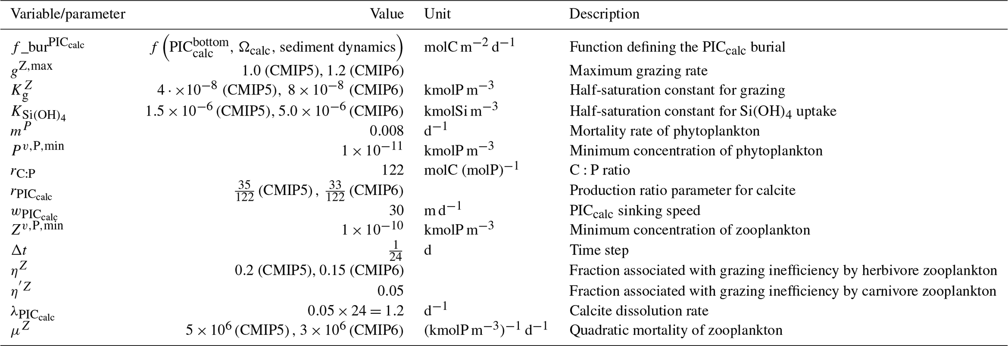
  PIC sinking speed: $w_{{\mathrm{PIC}}_{\mathrm{calc}}}$

•  

  PIC dissolution:

•  

  $\mathrm{Di}\left({\mathrm{PIC}}_{\mathrm{calc}}^v\right)=\min \left[\frac{\mathrm{PREREQ}}{\mathrm{\Delta }t},{\mathit{\lambda }}_{{\mathrm{PIC}}_{\mathrm{calc}}}\cdot {\mathrm{PIC}}_{\mathrm{calc}}^v\right]$

•  

  $\mathrm{PREREQ}=max\left(\mathrm{0},\frac{\left[{\mathrm{CO}}_{\mathrm{3}}^{\mathrm{2}-}\right]}{{\mathrm{\Omega }}_{\mathrm{calc}}}-\left[{\mathrm{CO}}_{\mathrm{3}}^{\mathrm{2}-}\right]\right)$

•  

  A dimension issue was noted.

•  

  Ballast effect: N/A

•  

  Protection effect: N/A

•  

  PIC burial:

•  

  $\mathrm{Bu}\left({\mathrm{PIC}}_{\mathrm{calc}}\right)=f\mathit{\_}{\mathrm{bur}}^{{\mathrm{PIC}}_{\mathrm{calc}}}$

C17 TOPAZ2

• Reference used: Dunne et al. (2013)

• Marine biogeochemical model of GFDL-ESM2G (CMIP5) and GFDL-ESM2M (CMIP5)

•  

  PIC balance:

•  

  $\frac{{\mathrm{DPIC}}_{\mathrm{calc}/\mathrm{arag}}^m}{\mathrm{D}t}=\mathrm{Pr}\left({\mathrm{PIC}}_{\mathrm{calc}/\mathrm{arag}}^m\right)-\mathrm{Di}\left({\mathrm{PIC}}_{\mathrm{calc}/\mathrm{arag}}^m\right)-w\cdot \frac{\partial {\mathrm{PIC}}_{\mathrm{calc}/\mathrm{arag}}^m}{\partial z}$

•  

  PIC export at 100 m:

•  

  Ex$\left({\mathrm{PIC}}_{\mathrm{calc}/\mathrm{arag}}\right)\left(\mathrm{100}\right)=\mathit{\rho }\cdot w\cdot {\mathrm{PIC}}_{\mathrm{calc}/\mathrm{arag}}^m\left(\mathrm{100}\right)$

•  

  PIC production:

•  

  $\mathrm{Pr}\left({\mathrm{PIC}}_{\mathrm{calc}}^{m,\mathrm{N}}\right)=r_{{\mathrm{PIC}}_{\mathrm{calc}}}\cdot r_{\mathrm{C}:\mathrm{N}}\cdot \exp \left(-\mathrm{0.0539}\cdot T\right)$

•  

  $\cdot min\left(\frac{\mathrm{1}}{\mathrm{\Delta }t},g_{\mathrm{0}}\cdot \exp \left(\mathrm{0.063}\cdot T\right)\cdot \frac{{\left(P_{\mathrm{small}}^{m,\mathrm{N}}\right)}^{\mathrm{2}}}{P_{\mathrm{small}}^g\cdot \left(P_{\mathrm{small}}^{m,\mathrm{N}}+P_{\mathrm{small}}^{{}^{\prime }g}\right)}\right)$

•  

  $\cdot P_{\mathrm{small}}^{m,\mathrm{N}}\cdot min\left[{\mathrm{\Omega }}^{\max },max\left(\mathrm{0},{\mathrm{\Omega }}_{\mathrm{calc}}-\mathrm{1}\right)\right]$

•  

  $\mathrm{Pr}\left({\mathrm{PIC}}_{\mathrm{arag}}^{m,\mathrm{N}}\right)=r_{{\mathrm{PIC}}_{\mathrm{arag}}}\cdot r_{\mathrm{C}:\mathrm{N}}\cdot min\left(\frac{\mathrm{1}}{\mathrm{\Delta }t},f\mathit{\_}{\mathrm{graz}}^{P_{\mathrm{large}}}\right)$

•  

  $\cdot P_{\mathrm{large}}^{m,\mathrm{N}}\cdot min\left[{\mathrm{\Omega }}^{\max },max\left(\mathrm{0},{\mathrm{\Omega }}_{\mathrm{arag}}-\mathrm{1}\right)\right]$

Table C17 TOPAZ2 parameters.

•  

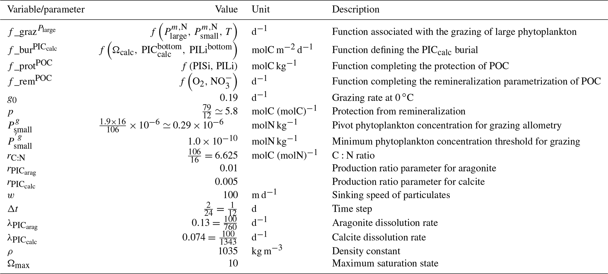
  PIC sinking speed: w

•  

  PIC dissolution:

•  

  $\mathrm{Di}\left({\mathrm{PIC}}_{\mathrm{calc}/\mathrm{arag}}^{m,\mathrm{N}}\right)={\mathit{\lambda }}_{{\mathrm{PIC}}_{\mathrm{calc}/\mathrm{arag}}}\cdot max\left(\mathrm{0},\mathrm{1}-{\mathrm{\Omega }}_{\mathrm{calc}/\mathrm{arag}}\right)$

•  

  $\cdot {\mathrm{PIC}}_{\mathrm{calc}/\mathrm{arag}}^{m,\mathrm{N}}$

•  

  Ballast effect: N/A

•  

  Protection effect:

•  

  $\mathrm{Re}\left({\mathrm{POC}}^{m,\mathrm{N}}\right)=f\mathit{\_}{\mathrm{rem}}^{\mathrm{POC}}\cdot max[\mathrm{0},{\mathrm{POC}}^{m,\mathrm{N}}$

•  

  $-\left(p\cdot \left({\mathrm{PIC}}_{\mathrm{calc}}^m+{\mathrm{PIC}}_{\mathrm{arag}}^m\right)+f\mathit{\_}{\mathrm{prot}}^{\mathrm{POC}}\right)]$

•  

  PIC burial:

•  

  $\begin{array}{l}\mathrm{Bu}\left({\mathrm{PIC}}_{\mathrm{calc}}\right)=f\mathit{\_}{\mathrm{bur}}^{{\mathrm{PIC}}_{\mathrm{calc}}}\\ \mathrm{Bu}\left({\mathrm{PIC}}_{\mathrm{arag}}\right)=\mathrm{0}\end{array}$

C18 BLINGv2

• Reference used: Dunne et al. (2020)

• Marine biogeochemical model of GFDL-CM4 (CMIP6)

•  

  PIC balance:

•  

  Ex$\left({\mathrm{PIC}}_{\mathrm{calc}}\right)\left(n\right)=min(\mathrm{1},n-\mathrm{1})\cdot \mathrm{Ex}\left({\mathrm{PIC}}_{\mathrm{calc}}\right)(n-\mathrm{1})$

•  

  $+\left[\mathrm{Pr}\left({\mathrm{PIC}}_{\mathrm{calc}}^m\right)\left(n\right)-\mathrm{Di}\left({\mathrm{PIC}}_{\mathrm{calc}}^m\right)\left(n\right)\right]\cdot \mathit{\rho }\cdot h\left(n\right)$

•  

  PIC export at 100 m: no specific calculation

•  

  PIC production:

•  

  $\mathrm{Pr}\left({\mathrm{PIC}}_{\mathrm{calc}}^m\left(n\right)\right)=r_{{\mathrm{PIC}}_{\mathrm{calc}}}\cdot r_{\mathrm{C}:\mathrm{P}}\cdot \left(\mathrm{1}-f\mathit{\_}{\mathrm{frac}}^{P_{\mathrm{large}}}\right)$

•  

  $\cdot \mathrm{Pr}\left(P^{m,\mathrm{P}}\left(n\right)\right)\cdot \exp (-\mathrm{0.0539}\cdot T)$

•  

  $\cdot min\left[{\mathrm{\Omega }}_{\mathrm{calc}}^{\max },max\left(\mathrm{0},{\mathrm{\Omega }}_{\mathrm{calc}}-\mathrm{1}\right)\right]$

•  

  PIC sinking speed: N/A

•  

  PIC dissolution:

•  

  $\mathrm{Di}\left({\mathrm{PIC}}_{\mathrm{calc}}^m\left(n\right)\right)=\left[\sum _{k=\mathrm{1}}^{n-\mathrm{1}}\left(\mathrm{Pr}\left({\mathrm{PIC}}_{\mathrm{calc}}^m\left(k\right)\right)-\mathrm{Di}\left({\mathrm{PIC}}_{\mathrm{calc}}^m\left(k\right)\right)\right)+\mathrm{Pr}\left({\mathrm{PIC}}_{\mathrm{calc}}^m\left(n\right)\right)\right]$

•  

  $\cdot \left[\mathrm{1}-\frac{\mathrm{1}}{\mathrm{1}+\frac{h\left(n\right)}{D_{{\mathrm{PIC}}_{\mathrm{calc}}}}\cdot min\left(\mathrm{1},\mathrm{1}-{\mathrm{\Omega }}_{\mathrm{calc}}\right)}\right]$

•  

  Ballast effect: N/A

•  

  Protection effect:

•  

  Ex$\left(\mathrm{POC}\right)(n+\mathrm{1})=\mathrm{Ex}\left(\mathrm{POC}\right)\left(n\right)+f\mathit{\_}{\mathrm{bal}}^{\mathrm{POC}}\left(n\right)$

•  

  PIC burial:

•  

  $\mathrm{Bu}\left({\mathrm{PIC}}_{\mathrm{calc}}\right)=f\mathit{\_}{\mathrm{bur}}^{{\mathrm{PIC}}_{\mathrm{calc}}}$

•  

  Bu(PIC_arag)=0

Table C18 BLINGv2 parameters.

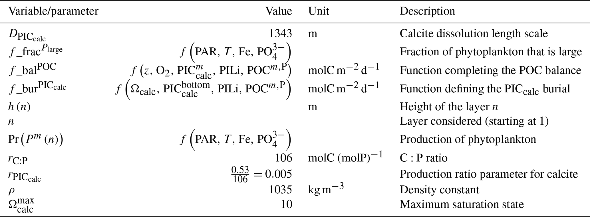
C19 COBALTv2

• References used: Stock et al. (2014, 2020)

• Marine biogeochemical model of GFDL-ESM4 (CMIP6)

•  

  PIC balance:

•  

  $\frac{{\mathrm{DPIC}}_{\mathrm{calc}/\mathrm{arag}}^m}{\mathrm{D}t}=\mathrm{Pr}\left({\mathrm{PIC}}_{\mathrm{calc}/\mathrm{arag}}^m\right)-\mathrm{Di}\left({\mathrm{PIC}}_{\mathrm{calc}/\mathrm{arag}}^m\right)$

•  

  $-w\cdot \frac{\partial {\mathrm{PIC}}_{\mathrm{calc}/\mathrm{arag}}^m}{\partial z}$

•  

  PIC export at 100 m:

•  

  Ex$\left({\mathrm{PIC}}_{\mathrm{calc}/\mathrm{arag}}\right)\left(\mathrm{100}\right)=\mathit{\rho }\cdot w\cdot {\mathrm{PIC}}_{\mathrm{calc}/\mathrm{arag}}^m\left(\mathrm{100}\right)$

•  

  PIC production:

•  

  $\mathrm{Pr}\left({\mathrm{PIC}}_{\mathrm{calc}}^m\right)=r_{{\mathrm{PIC}}_{\mathrm{calc}}}\cdot r_{\mathrm{C}:\mathrm{N}}\cdot min\left[{\mathrm{\Omega }}^{\max },max\left(\mathrm{0},{\mathrm{\Omega }}_{\mathrm{calc}}-\mathrm{1}\right)\right]$

•  

  $\cdot [{\mathit{\eta }}^{Z_{\mathrm{medium}}}\cdot f\mathit{\_}{{\mathrm{cons}}^{\prime }}^{Z_{\mathrm{small}}}\cdot Z_{\mathrm{small}}^{m,\mathrm{N}}+{\mathit{\eta }}^{Z_{\mathrm{small}}}\cdot f\mathit{\_}{{\mathrm{graz}}^{\prime }}^{P_{\mathrm{small}}}$

•  

  $\cdot P_{\mathrm{small}}^{m,\mathrm{N}}+{\mathit{\eta }}^{Z_{\mathrm{large}}}\cdot f\mathit{\_}{{\mathrm{graz}}^{\prime }}^{P_{\mathrm{large}}}\cdot P_{\mathrm{large}}^{m,\mathrm{N}}$

•  

  $+f\mathit{\_}{\mathrm{agg}}^{P_{\mathrm{small}}}\cdot P_{\mathrm{small}}^{m,\mathrm{N}}+f\mathit{\_}{\mathrm{agg}}^{P_{\mathrm{large}}}\cdot P_{\mathrm{large}}^{m,\mathrm{N}}]$

•  

  $\mathrm{Pr}\left({\mathrm{PIC}}_{\mathrm{arag}}^m\right)=r_{{\mathrm{PIC}}_{\mathrm{arag}}}\cdot r_{\mathrm{C}:\mathrm{N}}$

•  

  $\cdot min\left[{\mathrm{\Omega }}^{\max },max\left(\mathrm{0},{\mathrm{\Omega }}_{\mathrm{arag}}-\mathrm{1}\right)\right]$

•  

  $\cdot [{\mathit{\eta }}^{Z_{\mathrm{large}}}\cdot f\mathit{\_}{{\mathrm{cons}}^{\prime }}^{Z_{\mathrm{medium}}}\cdot Z_{\mathrm{medium}}^m+{\mathit{\eta }}^{\mathrm{hp}}$

•  

  $\cdot f\mathit{\_}{{\mathrm{hpcons}}^{\prime }}^{Z_{\mathrm{medium}}}\cdot Z_{\mathrm{medium}}^{m,\mathrm{N}}$

•  

  $+{\mathit{\eta }}^{\mathrm{hp}}\cdot f\mathit{\_}{\mathrm{hpcons}}^{{}^{\prime }{Z}_{\mathrm{large}}}\cdot Z_{\mathrm{large}}^{m,\mathrm{N}}]$

Table C19 COBALTv2 parameters.

•  

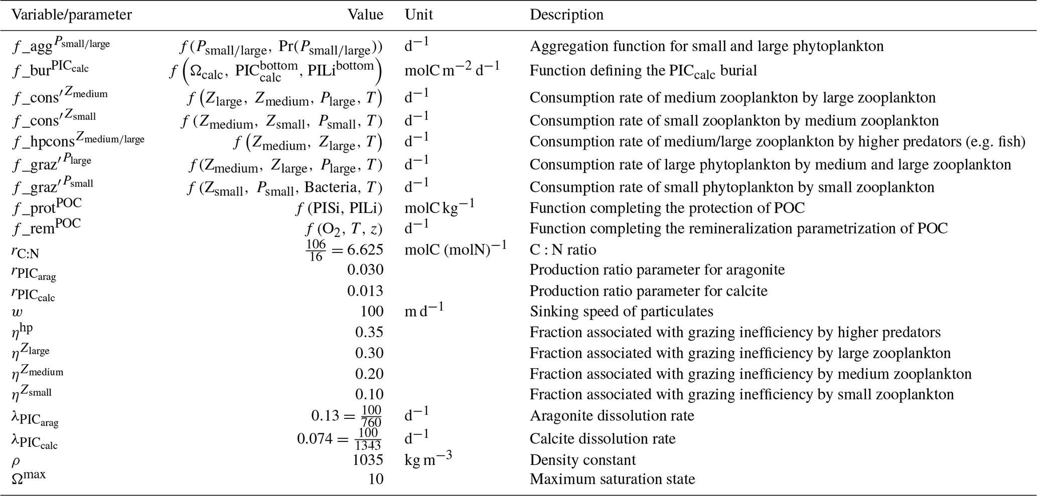
  PIC sinking speed: w

•  

  PIC dissolution:

•  

  $\mathrm{Di}\left({\mathrm{PIC}}_{\mathrm{calc}}^m\right)={\mathit{\lambda }}_{{\mathrm{PIC}}_{\mathrm{calc}/\mathrm{arag}}}\cdot max(\mathrm{0},\mathrm{1}-{\mathrm{\Omega }}_{\mathrm{calc}/\mathrm{arag}})$

•  

  $\cdot {\mathrm{PIC}}_{\mathrm{calc}/\mathrm{arag}}^m$

•  

  Ballast effect: N/A

•  

  Protection effect:

•  

  $\mathrm{Re}\left({\mathrm{POC}}^{m,\mathrm{N}}\right)=f\mathit{\_}{\mathrm{rem}}^{\mathrm{POC}}\cdot max[\mathrm{0},{\mathrm{POC}}^m$

•  

  $-\left(p\cdot \left({\mathrm{PIC}}_{\mathrm{calc}}^m+{\mathrm{PIC}}_{\mathrm{arag}}^m\right)+f\mathit{\_}{\mathrm{prot}}^{\mathrm{POC}}\right)]$

•  

  PIC burial:

•  

  $\mathrm{Bu}\left({\mathrm{PIC}}_{\mathrm{calc}}\right)=f\mathit{\_}{\mathrm{bur}}^{{\mathrm{PIC}}_{\mathrm{calc}}}$

•  

  Bu(PIC_arag)=0

Appendix D: Results and discussion

We share here additional figures that give a more detailed view of what is addressed in the main text.

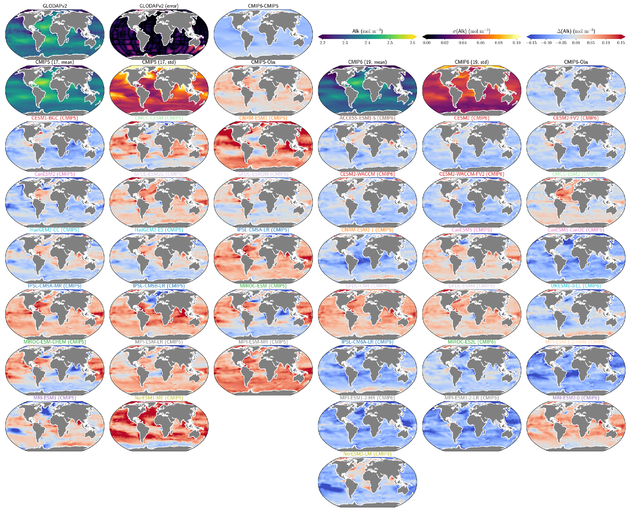
Figure D1 Alk surface distribution. ESM intercomparison of the open-ocean surface Alk as simulated by ocean biogeochemical models involved in CMIP5 (first three columns) and CMIP6 (last three columns) compared to GLODAPv2 observations. The first row gives the GLODAPv2 observational product, the associated error and the difference between the CMIP6 and CMIP5 ensemble means. The second row gives the ensemble mean, standard deviation, and observational bias for each CMIP.

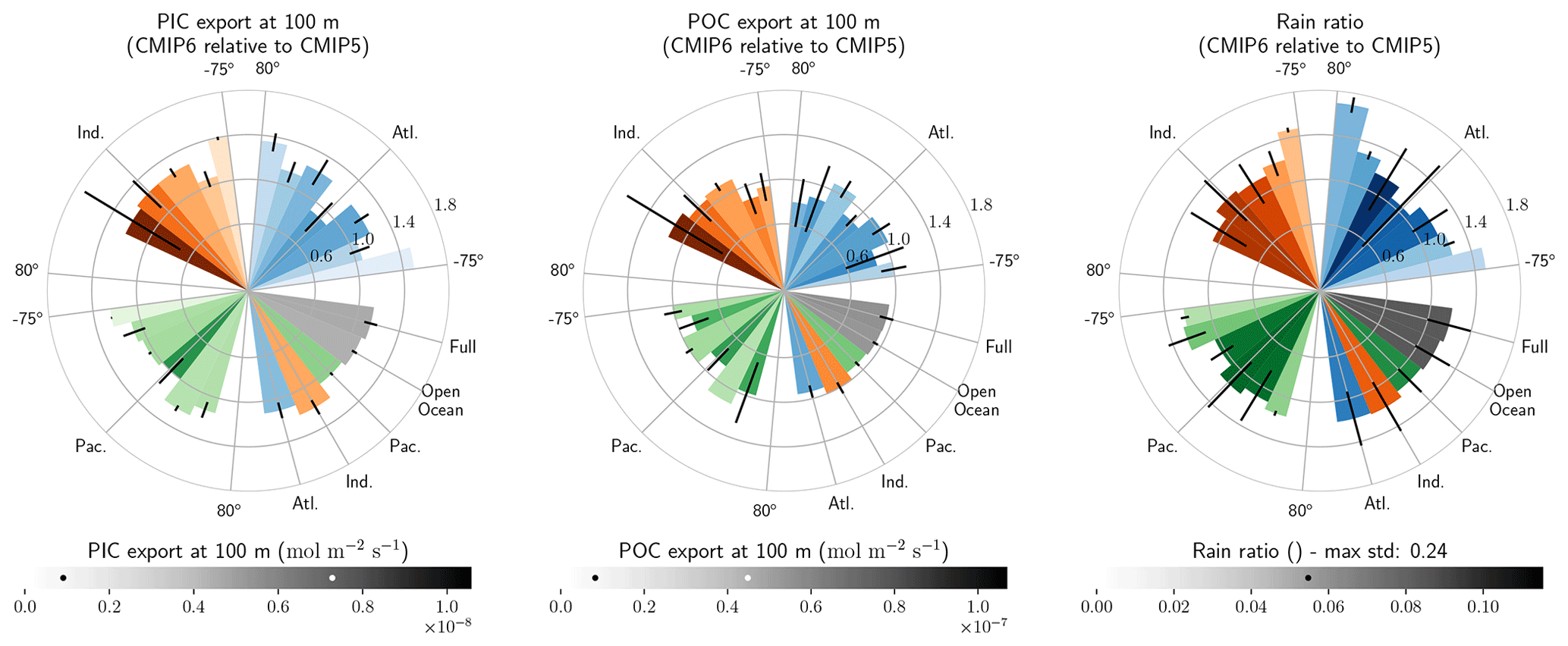
Figure D2 Spatial distribution of the PIC and POC exports at 100 m. The PIC export, POC export and rain ratio at 100 m for the Atlantic (blue), Indian (orange) and Pacific (green) basins and meridional sub-regions of each basin are shown. Bar heights give the relative difference between the CMIP6 and CMIP5 ensemble means. Bar colours give the CMIP6 ensemble mean (same shades as the grey-coloured bars). Errors are the CMIP6 standard deviation with values normalized between 0 and 0.5 (the minimum and maximum standard deviations are respectively marked by black and white points on the colour bars). Ocean basins are delineated as in Fig. A1.

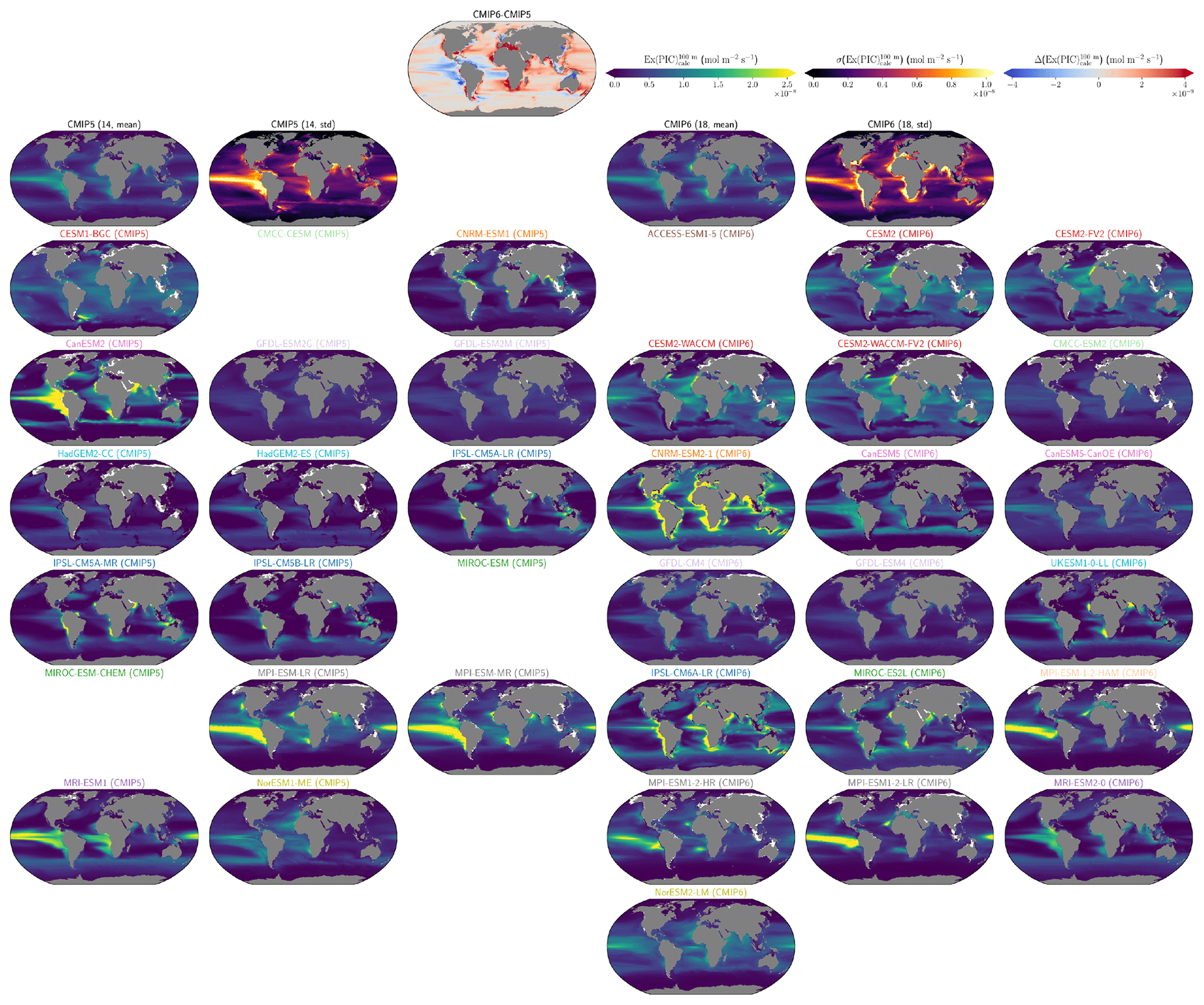
Figure D3 Distribution of the calcite export at 100 m. ESM intercomparison of the calcite export at 100 m as simulated by ocean biogeochemical models involved in CMIP5 (first three columns) and CMIP6 (last three columns). The first row gives the difference between the CMIP6 and CMIP5 ensemble means. The second row gives the ensemble mean and standard deviation for each CMIP.

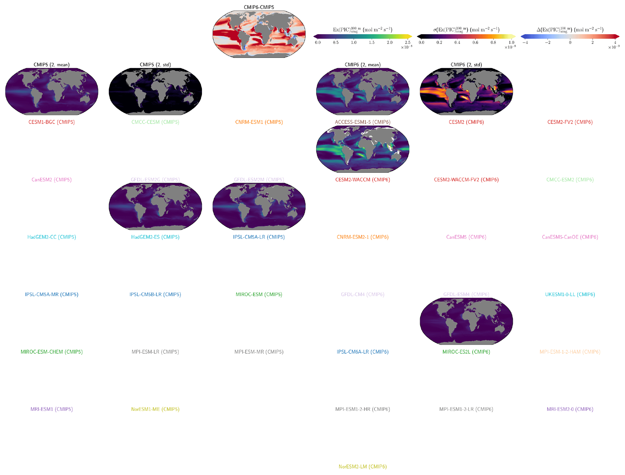
Figure D4 Like Fig. D3 but for the aragonite export at 100 m.

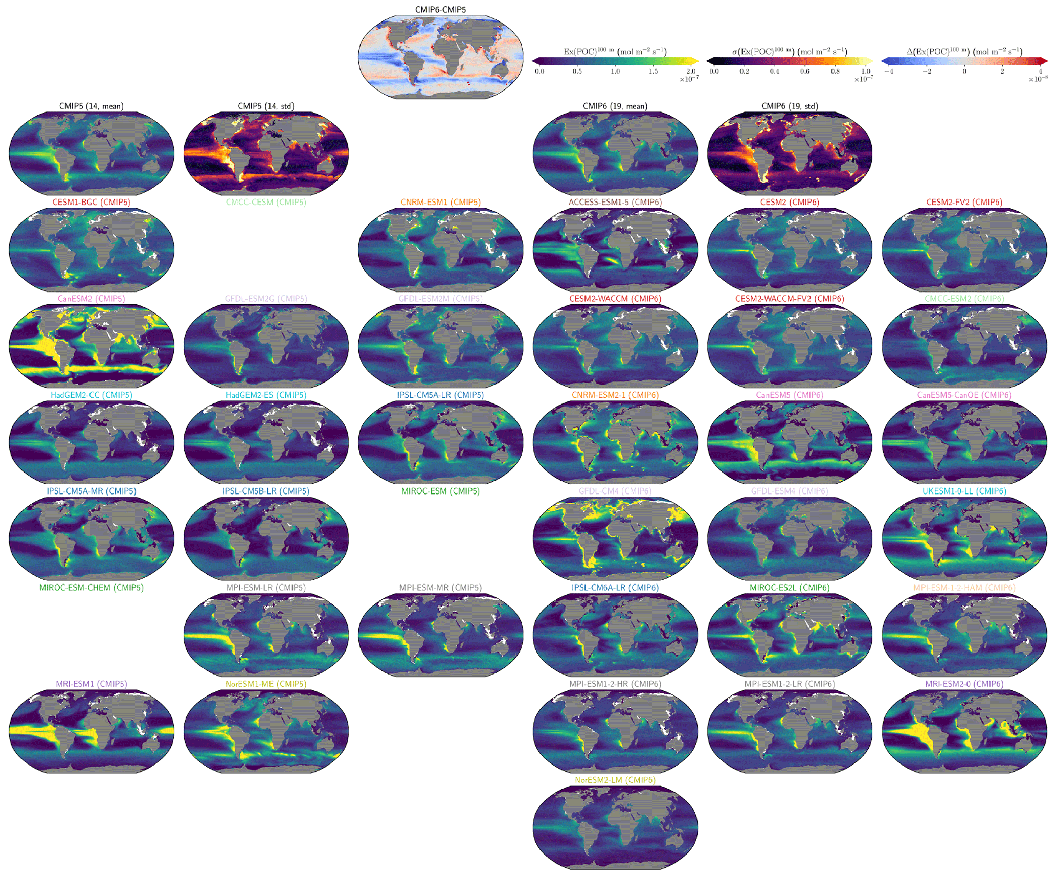
Figure D5 Like Fig. D3 but for the POC export at 100 m.

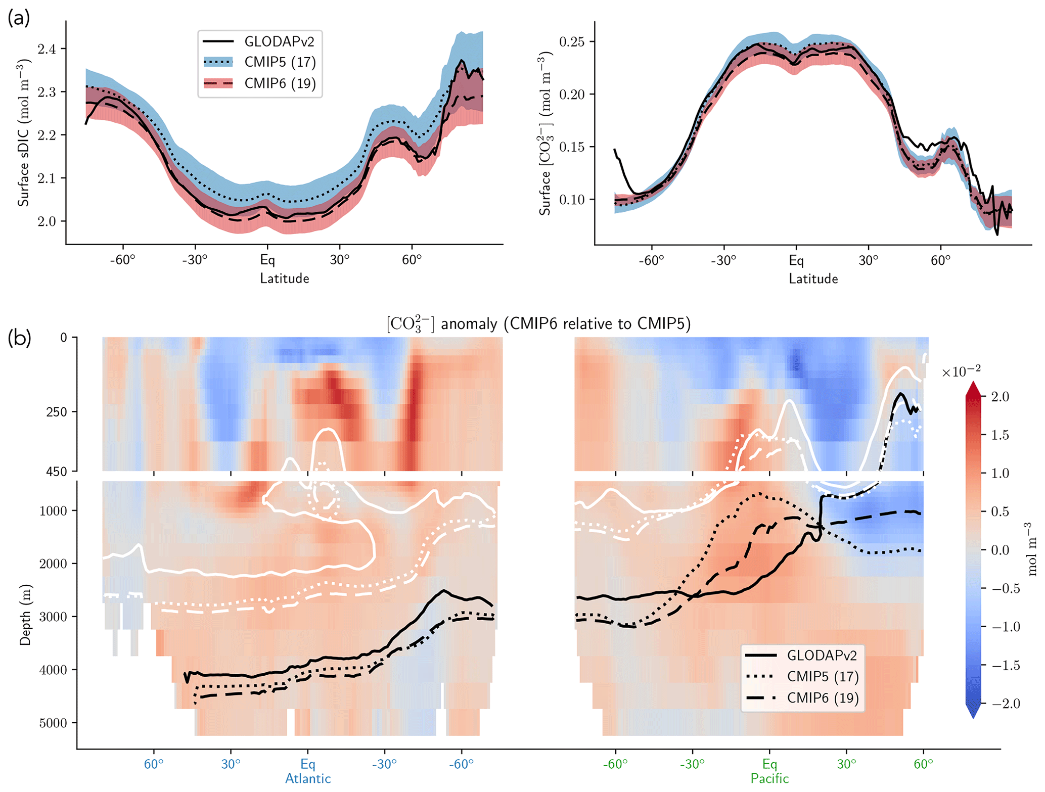
Figure D6 Complementary carbonate system assessment. (a) Open-ocean zonal averages of the surface sDIC (left) and carbonate ion concentration (right). (b) Atlantic–Pacific zonal average of the difference between the CMIP6 and CMIP5 ensemble means of the carbonate ion concentration. The saturation horizon depth for calcite (black lines) and aragonite (white lines) is shown for GLODAPv2 and CMIP5 and CMIP6 ensemble means.

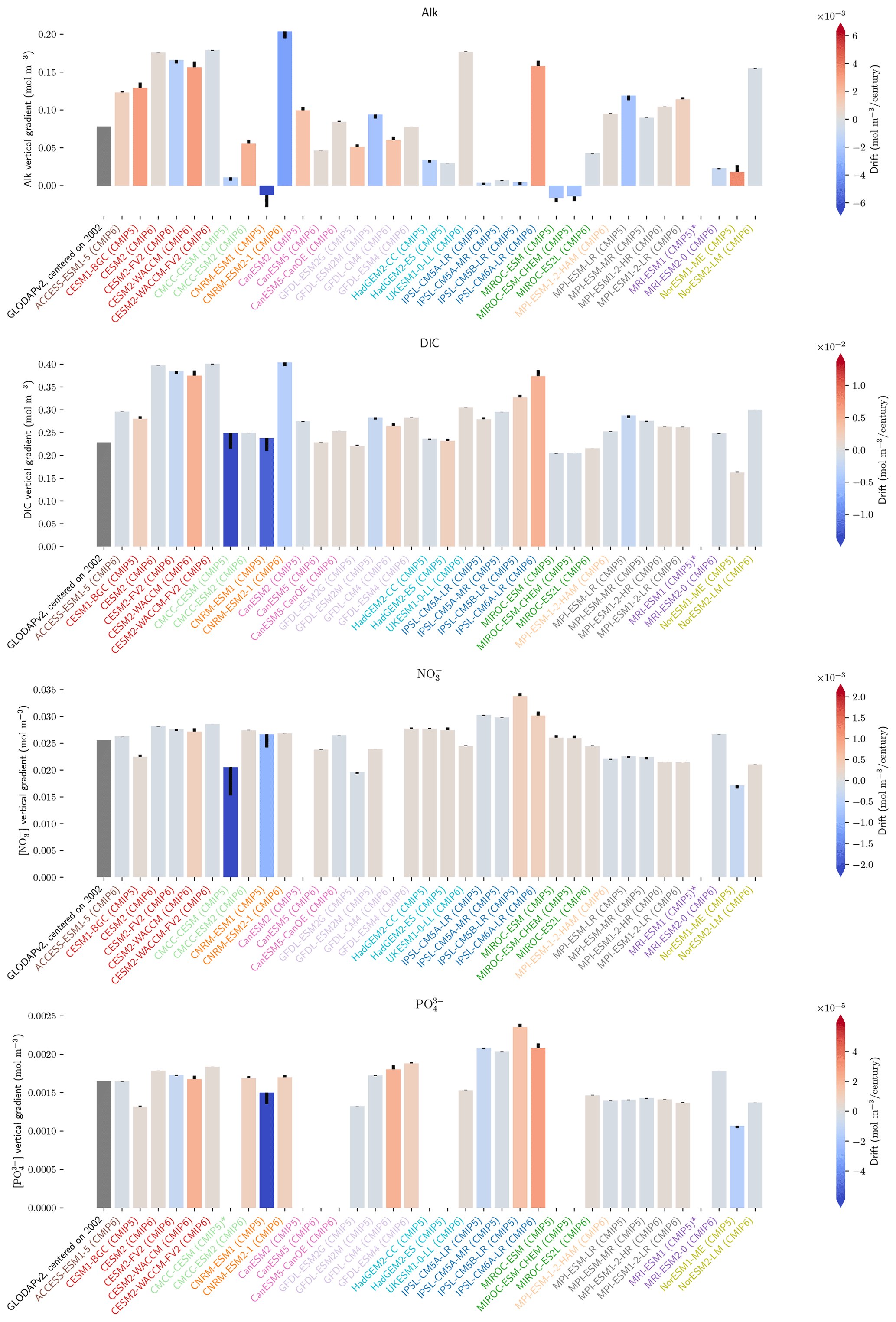
Figure D7 Additional CMIP5 and CMIP6 model drift evaluation. Drift in the global open-ocean vertical gradient (defined in Sect. 3.2.3) of Alk, DIC, nitrate and phosphate. For each panel, the first bar denotes the observations, bar height denotes the mean vertical gradient in the first 20 years of the piControl (corresponding to 1850–1870), and the extremity of the black bar denotes the mean vertical gradient in the last 20 years of the piControl (corresponding to ∼ 2080–2100). Bar colour denotes model drift per century. Model names with an asterisk are not shown due to extreme drift relative to other models. piControl data for MRI-ESM1 (CMIP5) and piControl nitrate data for CanESM2 (CMIP5) were not available.

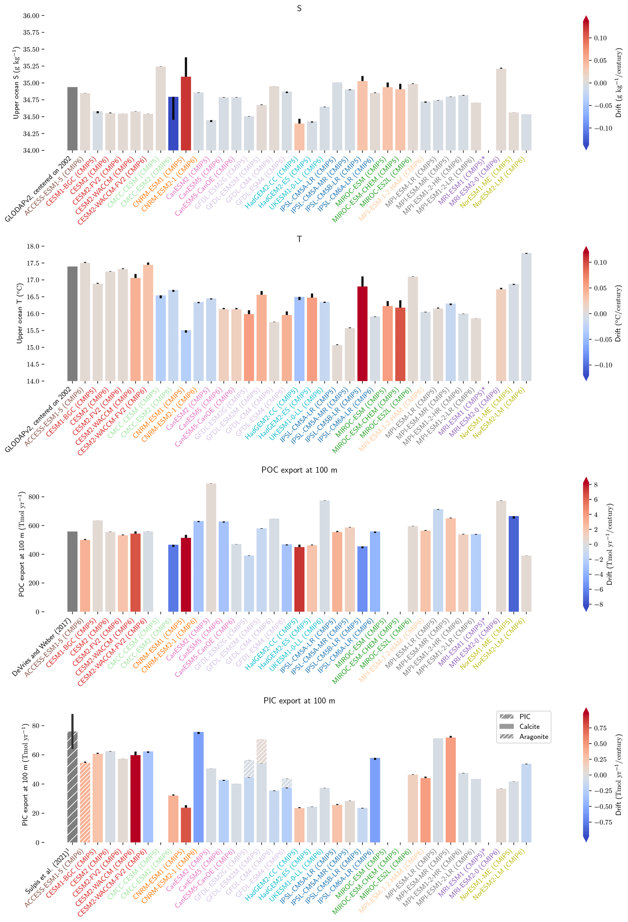
Figure D8 Additional CMIP5 and CMIP6 model drift evaluation (continuation of Fig. D7). Drift in upper (i.e. the first 100 m) open-ocean salinity and temperature (averaged between the surface and 100 m) as well as globally integrated POC and PIC (aragonite and calcite) export at 100 m. For each panel, the first bar denotes the observational estimates with the associated standard deviation for PIC export (¹assessment at 300 m). Bar height denotes the mean value in the first 20 years of the piControl (corresponding to 1850–1870), and the black bar denotes the mean value in the last 20 years of the piControl (corresponding to ∼ 2080–2100). Bar colour denotes model drift per century. Model names with an asterisk are not shown due to extreme drift relative to other models. piControl data for MRI-ESM1 (CMIP5) were not available.

Appendix E: GLODAPv2 observation

We discuss here the observations from GLODAPv2, since they seem to have a slight offset in either surface DIC or surface Alk compared to both CMIP5 and CMIP6 ensembles (see Fig. 12a). We have investigated whether the way we averaged the data around 2002 – as the observations from GLODAPv2 are normalized in 2002 – could drive a DIC offset, but this does not actually explain it. Indeed, we report that, to centre the data in 2002 regarding the ocean uptake of anthropogenic carbon, we should have in fact averaged from 1992 to between 2010 and 2011. Averaging between 1992 and 2012 induces a slight excess of DIC due to the non-linear increase in carbon uptake over this period. Although this excess in DIC is globally confined in the ocean surface layer, it does not impact our analysis, with an increase of less than 0.001 mol m⁻³ for all the ESMs at the surface ocean, which is negligible. A bias in the assessment of the Alk components that are diagnosed to compute the CO₂ system, especially the borate one, might drive a pCO₂ offset, resulting in a change in the y intercept in Fig. 12a (see Eq. 15) of a few millimole per cubic metre (Orr and Epitalon, 2015).

Similarly, we assessed the possible bias of using GLODAPv2 nutrients rather than the 2009 update of the WOA product (Boyer et al., 2018) which was available at the time of CMIP5 simulations. We report only a small difference between the observational products, essentially confined to deep waters, with a decrease of 3.8 % in the magnitude of the nitrate vertical profile at 5000 m (see Fig. 11b). Estimating the observed soft-tissue pump from the WOA product would therefore slightly reduce the bias between observations and the CMIP ESMs, with a globally negligible effect on our analysis of the vertical biases of sAlk and sDIC compared to the observations (see Fig. 9). The 10 % larger volume considered in WOA compared to GLODAPv2 (Lauvset et al., 2016) might partly explain the difference between the two data products at depth for nitrate and phosphate.

All that remains is to note the following biases in the observations and keep in mind their possible consequences: (i) many more observations are shared in the surface layer of the ocean than at depth, and in particular, the density of observations is divided by about 8 between the surface and the deep ocean. (ii) There are many more observations in both hemispheres during summer than winter. (iii) The spatial resolution of the gridded product is unequal, with excellent coverage of the North Atlantic Ocean and relatively bad coverage of the Southern Ocean (Olsen et al., 2020). In particular, this results in some important local common differences between the ESMs and GLODAPv2 (e.g. at high latitudes, where the ocean is seasonally covered by sea ice, and in the Weddell Sea especially).