Towards an ensemble-based evaluation of land surface models in light of uncertain forcings and observations

Quantification of uncertainty in fluxes of energy, water, and CO₂ simulated by land surface models (LSMs) remains a challenge. LSMs are typically driven with, and tuned for, a specified meteorological forcing data set and a specified set of geophysical fields. Here, using two data sets each for meteorological forcing and land cover representation (in which the increase in crop area over the historical period is implemented in the same way), as well as two model structures (with and without coupling of carbon and nitrogen cycles), the uncertainty in simulated results over the historical period is quantified for the Canadian Land Surface Scheme Including Biogeochemical Cycles (CLASSIC) model. The resulting eight ($\mathrm{2}\times \mathrm{2}\times \mathrm{2}$) model simulations are evaluated using an in-house model evaluation framework that uses multiple observation-based data sets for a range of quantities. The simulated area burned, fire CO₂ emissions, soil carbon mass, vegetation carbon mass, runoff, heterotrophic respiration, gross primary productivity, and sensible heat flux show the largest spread across the eight simulations relative to their global ensemble mean values. Simulated net atmosphere–land CO₂ flux, a critical determinant of the performance of LSMs, is found to be largely independent of the simulated pre-industrial vegetation and soil carbon mass, although our framework represents the historical increase in crop area in the same way in both land cover representations. This indicates that models can provide reliable estimates of the strength of the land carbon sink despite some biases in carbon stocks. Results show that evaluating an ensemble of model results against multiple observations disentangles model deficiencies from uncertainties in model inputs, observation-based data, and model configuration.

1 Introduction

The current-generation land surface models (LSMs) explicitly simulate the fluxes of energy, water, momentum, and trace gases (including CO₂, CH₄, and N₂O) between the atmosphere and the land surface. These models have become an essential tool in understanding what role the land surface plays in the global climate system under current and projected future changes in environmental conditions, including atmospheric CO₂ concentration (Bonan and Doney, 2018). LSMs are also an essential component of climate and Earth system models (ESMs), together with their ocean and atmosphere components. Within the framework of ESMs, LSMs are coupled interactively to their atmospheric components through the fluxes of energy, momentum, and matter.

The complexity of LSMs has increased over time, as more physical and biogeochemical processes have been included in their framework (Fisher and Koven, 2020; Kyker-Snowman et al., 2022). This increased complexity combined with the uncertainty in our understanding of physical and biogeochemical processes implies that different models respond differently even when driven with the same external forcings. One estimate of the uncertainty in our understanding of land surface physical and biogeochemical processes is obtained by evaluating the inter-model spread in a given quantity when models are forced in the same manner. Other than the uncertainty among models due to differences in their model structures and parameterizations of various processes, uncertainty also exists due to at least three other reasons. These include uncertainty (1) in parameter values¹ of represented processes, (2) in driving meteorological data, and (3) in the specification of the geophysical fields. LSMs are typically driven with meteorological data consisting of seven primary variables (incoming longwave and shortwave radiation, temperature, precipitation, specific humidity, wind speed, and pressure). In addition, the geophysical fields of land cover, soil texture, and soil permeable depth are also required. Driving data for LSMs also consist of atmospheric CO₂ concentration and other model-specific external forcings such as nitrogen deposition and fertilizer application rates for models that include a representation of the terrestrial nitrogen cycle and also lightning, population density, and gross domestic product (GDP) for models that simulate wildfires.

Every year, more than 15 land surface modelling groups participate in the TRENDY (trends in net land–atmosphere carbon exchanges) project where they perform a set of simulations that are driven with specified external forcings. The simulations are performed from the year 1700 to the present day. These simulations contribute to the annual Global Carbon Project's (GCP) analysis of the land carbon sink together with its analysis of anthropogenic CO₂ emissions and the ocean carbon sink (Friedlingstein et al., 2019). The external forcings used to drive LSMs in the TRENDY intercomparison include (1) 6-hourly meteorological data from 1901 to the present day (the most recent 2020 TRENDY intercomparison used the CRU-JRA forcing obtained by blending the Climatic Research Unit's (CRU) monthly data and the Japanese Reanalysis (JRA)), (2) atmospheric CO₂ concentration, and (3) information about changes in crop area and other land use change (LUC) from the land use harmonization (LUH) product (Hurtt et al., 2020). The information about changes in crop area and other LUC is used by land surface modelling groups to reconstruct historical land cover from the year 1700 to the present day consistently with the number of the plant functional types (PFTs) a given model represents. The protocol also provides nitrogen deposition and fertilization application rates for models including nitrogen cycling.

Models participating in the TRENDY simulations are thus driven with common meteorological and LUC forcings as part of their protocol. The resulting spread across models participating in the TRENDY project thus provides a measure of inter-model uncertainty, as mentioned earlier. Traditionally, the uncertainty associated with model structure has gained the most attention, and the scientific community has responded to this by performing model intercomparison projects (MIPs) where models are driven according to a common protocol. The Coupled Model Intercomparison Project (CMIP) in the climate community, together with its various sub-projects (Eyring et al., 2016), is another prominent example. MIPs now routinely form the basis of evaluating models against observations and multi-model means of various quantities. Multi-model means are also considered to be the best estimate for a given quantity (Tebaldi and Knutti, 2007).

The modelling community has been long aware of the uncertainty associated with parameter values, since a large fraction of physical and biogeochemical model processes are parameterized, and such uncertainty analysis dates back to the early hydrological models (e.g. Hornberger and Spear, 1981; Beven and Binley, 1992). More recent examples of parameter value uncertainty in the context of a given LSM include Poulter et al. (2010), Booth et al. (2012), and J. Li et al. (2018). The land surface modelling community, however, has only recently begun to address and quantify uncertainty related with driving meteorological data. Wu et al. (2017), for example, illustrate the uncertainty in gross primary productivity (GPP) simulated by the Lund–Potsdam–Jena General Ecosystem Simulator (LPJ-GUESS) model when driven by six different meteorological data sets. Bonan et al. (2019) analyze the uncertainty in simulated carbon-cycle-related variables using three versions of the Community Land Model (CLM) when driven with two meteorological data sets over the historical period. Slevin et al. (2017) assess the uncertainty in simulated GPP by the JULES land model when driven by three different meteorological data sets. Studies that evaluate the effect of different land cover representations on model performance are even fewer. Tian et al. (2004) and Lawrence and Chase (2007) study the effect of new land surface boundary conditions, including leaf area index and fractional vegetation cover, based on the MODIS satellite data as implemented in CLM2 in the Community Atmosphere Model (CAM2) and CLM3 in the Community Climate System Model (CCSM 3.0), respectively.

Here, we drive the Canadian Land Surface Scheme Including Biogeochemical Cycles (CLASSIC) with two sets of historical meteorological forcings and also two land cover representations to quantify the uncertainty associated with both these forcings. Other than these, we also use two versions of the CLASSIC model: one that represents the interactions between the carbon (C) and nitrogen (N) cycles and another in which these interactions are turned off. CLASSIC has contributed to the simulations for the TRENDY intercomparison, and the GCP, since 2016 (formerly under the CLASS-CTEM name). Seiler et al. (2021) have evaluated how well the CLASSIC model performs when forced with three different meteorological data sets using the model version without the N cycle. Using the two meteorological forcing data sets, two representations of land cover, and two versions of the model, we perform eight simulations over the historical period since 1700. All of these simulations may be considered equally likely representations of the modelled state of the land surface over the historical period. Yet, they all have their own distinct biases, since simulated land surface states and fluxes are different. We use these simulations to illustrate the uncertainty associated with meteorological forcing and the two different representations of land cover that are used to drive the model. We also use an in-house open-source benchmarking system (see code and data availability section) to evaluate these different simulations against observation-based data sets: AMBER (Automated Benchmarking R package; Seiler et al., 2021) uses gridded and in situ observation-based estimates of 19 energy-, water-, and C-cycle-related variables to evaluate LSMs.

Section 2 of this paper describes the framework of the CLASSIC land model and the forcing data that are required to drive the model. Section 3 describes the two meteorological data sets, the two representations of land cover that are used to drive the model, and the simulations performed for this study. Section 4 analyzes the results from the simulations to illustrate their different states and reports results from the AMBER benchmarking exercise. Finally, the discussion and conclusions are presented in Sect. 5. The use of more than one meteorological forcing data set and land cover representation yields a conundrum, since tuning model parameters for a given forcing data set is not a useful exercise anymore. We also report a new finding that, despite different land C states (characterized in terms of vegetation and soil C mass) in the eight simulations considered here, the net atmosphere–land CO₂ flux over the historical period in these simulations is consistent with estimates from the GCP. This and the discussion about the broader question of model tuning are also presented in Sect. 5.

2 The CLASSIC land modelling framework

2.1 The physical and carbon biogeochemical processes

The CLASSIC land model is the successor to and is based on the coupled Canadian Land Surface Scheme (CLASS; Verseghy, 1991; Verseghy et al., 1993) and the Canadian Terrestrial Ecosystem Model (CTEM; Arora and Boer, 2005; Melton and Arora, 2016). CLASSIC also serves as the land component in the family of Canadian Earth system models (Arora et al., 2009, 2011; Swart et al., 2019). Melton et al. (2020) provide an overview of the CLASSIC land model and launched it as a community model. The basis of the modelling of physical and biogeochemical processes in CLASSIC comes from CLASS and CTEM, respectively, both of which have a long history of development. CLASSIC simulates land–atmosphere fluxes of water, energy, and momentum based on its physics and fluxes of CO₂, CH₄, N₂O, NO_x, and NH₃ based on its biogeochemical process. The representation of the terrestrial N cycle is a new addition to CLASSIC (Asaadi and Arora, 2021; Kou-Giesbrecht and Arora, 2022) and allows for the simulation of the interactions between the C and N cycles explicitly.

The CLASSIC model simulations can be performed over a spatial domain, which may be global or regional, using gridded data or at a point scale, e.g. using meteorological and geophysical data from a FLUXNET site. The primary physical and biogeochemical processes of CLASSIC are briefly summarized in the next two sections.

2.1.1 Physical processes

The calculations for physical processes in CLASSIC are performed over vegetated, snow, and bare fractions at a time step of 30 min. In the version used here, the fractional coverage of the four plant functional types (PFTs; needleleaf trees, broadleaf trees, crops, and grasses) characterizes vegetation for each grid cell. The fractional coverage of these four PFTs is specified over the historical period in this study. The structure of vegetation is characterized by leaf area index (LAI), vegetation height, canopy mass, and rooting distribution through the soil layers, all of which are dynamically simulated by the biogeochemical module of CLASSIC. Twenty ground layers represent the soil profile, starting with 10 layers of 0.1 m thickness. The thickness of layers gradually increases to 30 m for a total ground depth of over 61 m. The depth of permeable-soil layers and thus the depth to bedrock varies geographically and is specified based on the SoilGrids250m data set (Hengl et al., 2017). Liquid and frozen soil moisture contents and soil temperature are determined prognostically for permeable soil layers. The temperature, albedo, mass, and density of a single-layer snow pack (when the climate permits snow to exist) are also prognostically modelled. The result of physics calculations yields fluxes of energy (primarily net radiation, ground heat flux, and latent and sensible heat fluxes) and water (primarily evapotranspiration and runoff) at the land–atmosphere boundary.

2.1.2 Biogeochemical processes

The biogeochemical processes in CLASSIC, based on CTEM, are described in detail in the Appendix of Melton and Arora (2016). The biogeochemical processes simulate the land–atmosphere exchange of CO₂ and as a result simulate vegetation as a dynamic component depending on the environmental conditions.

The biogeochemical module of CLASSIC prognostically calculates the amount of C in the model's three live (leaves, stem, and root) and two dead (litter and soil) C pools for each PFT. The live-vegetation pools are separated into their structural and non-structural components. The C amount in these pools is represented per unit of land area (kg C m⁻²). The amount of C in the live and dead C pools and all terrestrial ecosystem processes in the biogeochemical module in this study are modelled for nine PFTs that map directly onto the four base PFTs used in the physics module of CLASSIC. Needleleaf trees are divided into their deciduous and evergreen phenotypes; broadleaf trees are divided into cold-deciduous, drought-deciduous, and evergreen phenotypes; and crops and grasses are divided based on their photosynthetic pathways into C₃ and C₄ versions. The physical processes in CLASSIC are less sensitive to this sub-division of PFTs which is essential for modelling biogeochemical processes. For instance, simulating the onset and offset of leaves is different between evergreen and deciduous phenotypes of needleleaf and broadleaf trees, and this is simulated in the biogeochemical module of the model. However, once the leaf area index (LAI) is known, the physical processes in CLASSIC do not need information about the underlying deciduous or evergreen nature of leaf phenology. For example, the interception of rain and snow by canopy leaves (that is typically modelled as a function of LAI and is a PFT-dependent parameter that accounts for leaf orientation and shape) does not depend on the underlying evergreen or deciduous nature of the leaf phenology. In general, biogeochemical processes benefit more in terms of realism than physical processes do when the number of PFTs is increased. For example, in offline CLASSIC simulations, large changes in leaf area index (LAI) do not change total latent heat flux considerably, since the partitioning of evapotranspiration into its sub-components (transpiration, soil evaporation, and evaporation and/or sublimation of intercepted rain and/or snow) adjusts. A decrease in transpiration and evaporation of intercepted precipitation due to a decrease in LAI is compensated for by an increase in soil evaporation. This is expected, since water and energy fluxes are determined largely by available energy and precipitation.

The litter and soil C pools are tracked for each soil layer, but the movement of C between the soil layers is not yet modelled. Other than photosynthesis and leaf respiration, which are modelled at a time step of 30 min, all other biogeochemical processes are modelled at a daily time step. These include the following: (1) allocation of C from leaves to stem and roots, (2) autotrophic respiration from the live C pools and heterotrophic respirations from the dead C pools, (3) leaf phenology, (4) turnover of live-vegetation components that generates litter, (5) mortality, (6) LUCs, and (7) fire (Arora and Melton, 2018). Competition between PFTs for space is not modelled in this study, and fractional coverage of the nine PFTs is specified based on the representation of the land cover as explained in the next section.

When the N cycle is turned on, land–atmosphere fluxes of N₂O, NO_x, and NH₃ and N leaching are also modelled in response to biological N fixation, N fertilizer inputs, and N deposition from the atmosphere. In particular, when the N cycle interacts with the C cycle, the maximum photosynthetic capacities of model PFTs (V_c,max) are determined prognostically as a function of their leaf N content (Asaadi and Arora, 2021; Kou-Giesbrecht and Arora, 2022). When the N cycle is turned off, prescribed PFT-specific V_c,max rates are used (Melton and Arora, 2016), and an empirical downregulation parameterization is used to emulate the effect of nutrient constraints as atmospheric CO₂ increases (Arora et al., 2009). N in all model components (leaves, stem, roots, litter, and soil organic matter) is prognostically tracked, and therefore the C:N ratio of all components is prognostically modelled except for that of soil organic matter, for which a C:N ratio of 13 is specified. In addition, N in the soil mineral pools of nitrate (NO${}_{\text{3}}^{-})$ and ammonium (NH${}_{\text{4}}^{+})$ is also prognostically modelled.

3 Driving data for CLASSIC and model simulations

3.1 Land cover

Land cover is one of the most important geophysical fields that is required by LSMs and that, at its most basic level, provides information about fractional vegetation cover in each grid cell for a given regional or global domain. Vegetation in LSMs is typically represented in terms of PFTs. Models may choose to represent a basic set of a few PFTs (trees, grasses, shrubs, and crops) or a more elaborate set that distinguishes PFTs based on their stature (trees, grasses, or shrubs), leaf form (needleleaf or broadleaf), leaf phenology (evergreen or deciduous), photosynthetic pathway (C₃ or C₄), and geographical location (tropical, temperate, or boreal). The version of CLASSIC in this study uses a somewhat smaller set of nine PFTs for biogeochemical processes, as described in the previous section. The fractional coverage of PFTs in a model may be dynamically simulated based on competition between PFTs or prescribed based on observation-based land cover information. While CLASSIC does have a parameterization of competition between its PFTs (Arora and Boer, 2006; Melton and Arora, 2016), for the historical simulations considered here and for the simulations that contribute to the TRENDY ensemble, prescribed fractional coverage of PFTs is used.

For the process of generating a historical reconstruction of land cover consisting of time-varying fractional coverage of a model's PFTs two types of observation-based data sets are used. The first is a remotely sensed land cover product that represents the geographical distribution of land cover for the present day for a short period. Examples of this include the GLC 2000 land cover product which represents the November 1999 to December 2000 period (https://forobs.jrc.ec.europa.eu/products/glc2000/glc2000.php. last access: July 2022) and the more recent European Space Agency (ESA) Climate Change Initiative (CCI) land cover product for the period 1992–2018 (ESA, 2017). The second type of data set required to reconstruct historical land cover is that of a spatially and temporally varying cropland (and pasture) area for a much longer period, which in this case is based on the data set provided by the land use harmonization (LUH) product as part of the TRENDY protocol for the period 850–2018. The LUH product is comprehensive (Hurtt et al., 2020). For example, not all models use the pasture area and other information provided in the LUH product.

The process of generating land cover for a given model's PFTs is a three-step process. First, the fractional coverage of model PFTs is obtained from a remotely sensed land cover product that represents the snapshot of land cover for the present day. This requires typically mapping 20–40 land cover classes that exist in a remotely sensed land cover product to a given model's PFTs. This step introduces the largest uncertainty in the entire process. The original land cover in the CLASSIC model is based on the GLC 2000 land cover product. Table 2 of Wang et al. (2006) summarizes the mapping and reclassification of the 22 GLC 2000 land cover categories to the nine PFTs used in CLASSIC. Each land cover class was split into one or more of the nine CLASSIC PFTs based on the class description and knowledge of global biomes. For example, the discrete “broadleaf deciduous open tree cover” category of the GLC 2000 product is assumed to consist of 60 % broadleaf deciduous trees, 20 % grasses, and 20 % bare ground. This first step yields a snapshot of land cover expressed in terms of the fractional coverage of CLASSIC's nine PFTs corresponding to the time associated with the land cover product (e.g. for year 2000 for the GLC 2000 land cover product). The second step of generating fractional coverage of PFTs for a given snapshot in time requires replacing the fractional area of crop categories with values from the LUH data set for the same year. For example, when using the GLC 2000 land cover product, the area of C₃ and C₄ crops from the LUH data set for the year 2000 are used, and the fractional coverage of the other seven non-crop CLASSIC PFTs is adjusted such that the total vegetation fraction in each grid cell stays the same. Finally, in the last step, the temporally varying crop area from the LUH product is used to go backward in time to 1700 from the year 2000 with typically decreasing crop area, while the area of other non-crop PFTs is adjusted in proportion to their existing fractional coverage such that the total vegetation fraction in each grid cell stays the same. Similarly, the area of C₃ and C₄ crops from the LUH product is used from the year 2000 onwards to the present day with changing crop area, and the area of non-crop PFTs is adjusted such that the total vegetation fraction in each grid cell stays the same. All these steps yield a reconstruction of historical land cover, expressed in terms of fractional coverage of CLASSIC's nine PFTs (as interpreted from the GLC 2000 land cover product) from 1700 to 2018, in which crop area changes spatially and temporally according to the LUH product.

GLC 2000 is an older land cover product, and more recent land cover products are now available. Here, in addition to the GLC-2000-based land cover, we also use the European Space Agency (ESA) Climate Change Initiative's (CCI) land cover product. The ESA CCI land cover product is available at 300 m spatial resolution for the period 1992–2018 and contains 37 land cover categories (ESA, 2017). We use the land cover from the year 1992 to create a snapshot of CLASSIC PFTs for the present day. Although there is some interannual variability overall, the total vegetated area does not change substantially from 1992–2018 in the ESA-CCI land cover. A default mapping and reclassification table for converting the ESA CCI classes into PFTs is provided in its user guide (ESA, 2017). However, it overestimates tree cover along the taiga–tundra transition zone and underestimates it elsewhere in Canada (Wang et al., 2018, 2019). Wang et al. (2022) have developed a new reclassification table for converting the 37 ESA CCI land cover categories to CLASSIC's nine PFTs which are used in this study. A high-resolution land cover map over Canada and tree cover fraction data at 30 m resolution are used to compute the sub-pixel fractional composition of each class in the ESA CCI data set, which is then used to inform the cross-walking reclassification procedure (Wang et al., 2022).

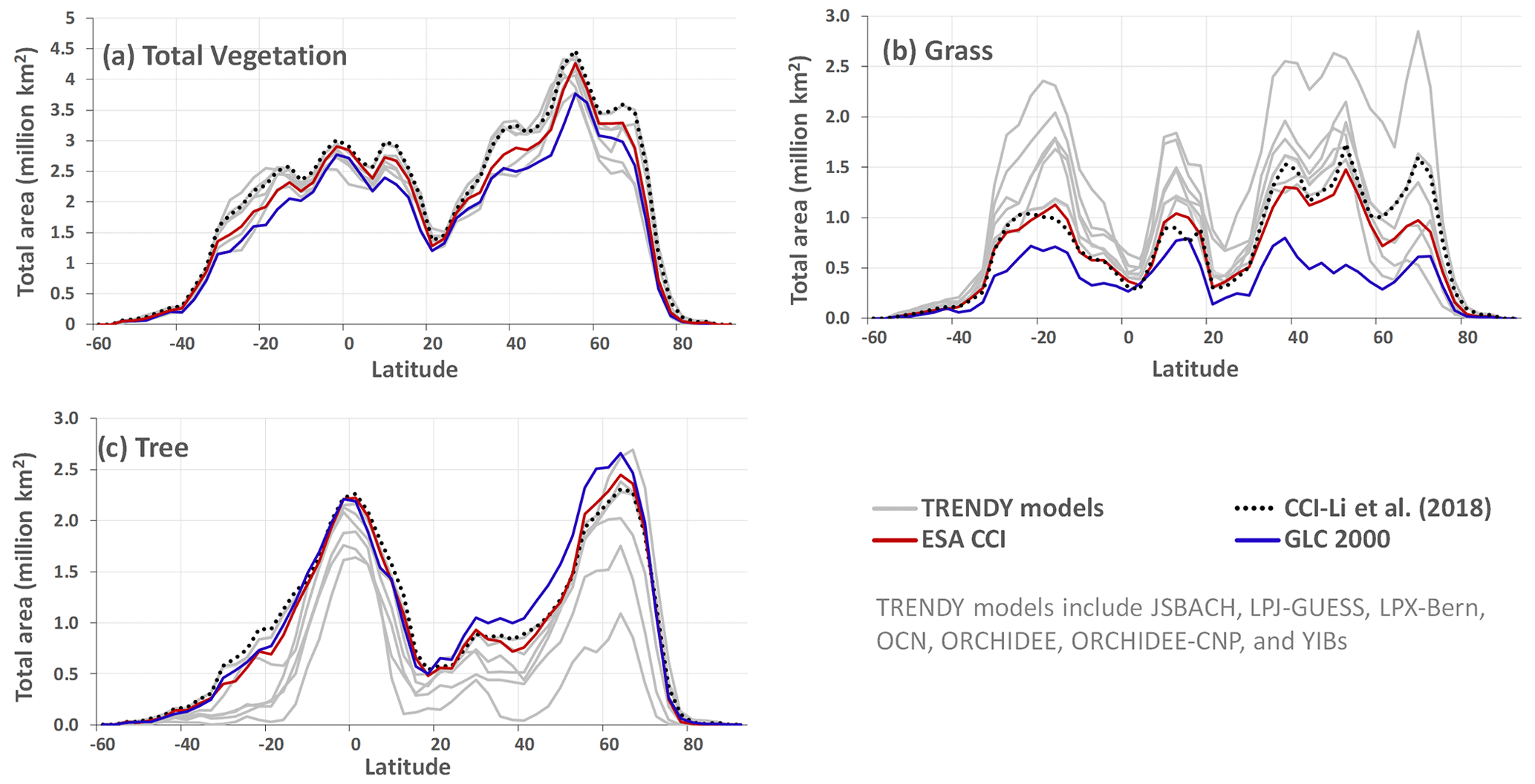
Figure 1 Comparison of zonally summed areas of total vegetation (a), grass (b), and tree (c) cover used in the CLASSIC model based on GLC 2000 (blue line) and ESA CCI (dark red line) land cover products to each other; to selected other models that participated in the 2020 TRENDY intercomparison (grey lines) for which land cover information was available; and to W. Li et al. (2018; dotted black line), who analyzed the ESA CCI data. All data correspond to the 1992–2018 period. CLASSIC does not yet explicitly represents shrub PFTs. Tall shrubs are merged into tree PFTs in CLASSIC. For the W. Li et al. (2018) data plotted here, the shrub PFTs are combined with the tree PFTs for a consistent comparison to CLASSIC.

The above process yields two representations of land cover in which the geographical distribution of CLASSIC PFTs is based on GLC 2000 and ESA CCI land cover products. Both these representations include the same reconstruction of crop area over the historical period. Figure 1 illustrates the uncertainty in land cover by comparing zonally summed areas of total vegetation, tree, and grass cover in CLASSIC, averaged over the period 1992–2018, when model land cover is based on the GLC 2000 (blue line) and ESA CCI (dark red line) land cover products. These two estimates are also compared to selected other models that participated in the 2020 TRENDY intercomparison (grey lines), also for the period 1992–2018, for which land cover information was available and also to W. Li et al. (2018) (dotted black line), who analyzed the ESA CCI data based on the default reclassification table from the ESA CCI user guide. Figure 1 shows that, while there is relatively good agreement across TRENDY models in terms of total vegetation cover, there's a much larger uncertainty in its split between tree and grass PFTs. There are two reasons for the spread in total vegetated, treed, and grassed areas across TRENDY models. First, modelling groups use different remotely sensed land cover products for obtaining fractional cover of their model PFTs. Second, the current process of mapping and reclassifying 20–40 land cover classes of a land cover product to a model's PFTs is mainly based on the class description and expert judgement, which introduces subjectiveness into the process. Compared to the GLC-2000-based land cover in the CLASSIC model, the newer ESA-CCI-based land cover yields a somewhat higher total vegetation cover, a higher grass cover, and a somewhat lower tree cover area. Unlike the older GLC-2000-based land cover used in CLASSIC, the newer ESA-CCI-based grass and tree cover areas are within the range of the TRENDY models reported here. Finally, Fig. 1 also allows us to compare the results from the analysis of W. Li et al. (2018) for the ESA CCI land cover (dotted black line) to the ESA CCI reclassification for CLASSIC (dark red line) by Wang et al. (2022). W. Li et al. (2018) used the default mapping and reclassification table for converting the ESA CCI classes into PFTs. This comparison illustrates that the remapping of the ESA CCI land cover classes to CLASSIC's PFTs yields total vegetation, tree, and grass coverage that is broadly comparable to that of W. Li et al. (2018), although some differences remain for the grasses.

Our framework accounts for the uncertainty in land cover representation. However, since both land cover representations in our study account for the increase in crop area over the historical period in the same way by adjusting the area of non-crop PFTs in proportion to their existing coverage using the LUH product, our framework is unable to account for the uncertainty associated with the implementation of LUCs. Di Vittorio et al. (2018) quantify this uncertainty by implementing several approaches to account for the increase in crop area over the historical period in the framework of an integrated assessment model: preferentially converting grasses and shrubs, preferentially converting forests, and proportionally adjusting areas of non-crop PFTs in a way that is similar to ours. LUC emissions are higher if the increase in crop area is preferentially obtained by converting forests. A similar uncertainty analysis for LUC emissions is performed by Peng et al. (2017) who, using the ORCHIDEE land model, analyze the effect of using different rules to incorporate the changes in crop and pasture area over the historical period. The uncertainty related to incorporating LUC information to modify a model's land cover is further illustrated in Di Vittorio et al. (2014) and Meiyappan and Jain (2012).

3.2 Meteorological data

As a land surface component of an ESM, CLASSIC requires meteorological forcing at a sub-daily temporal resolution. In the offline simulations reported here, the model is run with half-hourly values of meteorological data (incoming longwave and shortwave radiation, temperature, precipitation, specific humidity, wind speed, and pressure). The first meteorological data set used to drive CLASSIC is from the TRENDY protocol for the year 2020, CRU-JRA v2.1.5, which provides 6-hourly values of the seven variables from the Japanese Reanalysis (JRA) with monthly values adjusted to the Climatic Research Unit's data (CRU; https://crudata.uea.ac.uk/cru/data/hrg/. last access: July 2022). This yields a blended product from January 1901 to December 2018 with the 6-hourly temporal resolution of a reanalysis but without the biases that may be present in reanalysis data (Harris, 2020). The second meteorological data set used here to drive CLASSIC is from the Global Soil Wetness Project 3 (GSWP3). The GSWP3 forcing data are based on a dynamical downscaling of the 20th-century reanalysis (Compo et al., 2011) using a global spectral model (GSM) run at about 50 km resolution. The GSM is nudged towards the vertical structures of 20th-century (20CR) zonal and meridional air temperature and winds so that the synoptic features are retained at their higher spatial resolution. Additional bias corrections are also performed as explained in van den Hurk et al. (2016). The GSWP3 forcing is available for the 1901–2016 period. The 6-hourly values from both the CRU-JRA and GSWP3 forcings are further disaggregated to half-hourly values for use by CLASSIC.

Figure A1 in the Appendix compares the two meteorological forcing data sets over the 1997–2016 period to illustrate that although these two data sets are very similar, there are differences between the two. Mean annual global precipitation over land (excluding Greenland and Antarctica) in the GSWP3 data set (71.4 mm month⁻¹, 857 mm yr⁻¹) is somewhat higher than in the CRU-JRA data set (68.3 mm month⁻¹, 820 mm yr⁻¹). The global near-surface air temperature over land (excluding Greenland and Antarctica) is also slightly higher in the GSWP3 data set (14.22 ^∘C) compared to in the CRU-JRA data set (14.08 ^∘C). The largest temperature difference occurs between the two data sets over the northern tropics (panel h) where the GSWP3 data set is about 0.93 ^∘C warmer than the CRU-JRA data set. The geographical distribution of mean annual temperature is very similar between the two data sets, but there are some differences in the geographical distribution of precipitation (not shown). Despite very similar total precipitation amounts and their seasonality over large global regions in the two data sets, differences exist in the frequency distribution of precipitation. Figure A2 illustrates this over three broad regions, the Amazon, the Sahel, and the Midwest United States, showing the frequency distribution of daily precipitation amounts (mm d⁻¹) over the 1997–2016 period from the two data sets. Figure A2 shows that the frequency of precipitation events greater than about 5–10 mm d⁻¹ is higher in the GSWP3 data set compared to in the CRU-JRA data set for the Amazonian, the Sahel, and the Midwest United States regions.

3.3 Other forcings

Other than the land cover and meteorological forcings, CLASSIC requires globally averaged atmospheric CO₂ concentration; geographically varying, time-invariant soil texture and soil permeable depth; population density; monthly climatological lightning; and geographically and time-varying N fertilizer application rates and atmospheric N deposition rates. The atmospheric CO₂ concentration values are provided by the TRENDY protocol. The soil texture information consists of the percentage of sand, clay, and organic matter and is derived from Shangguan et al. (2014). N fertilizer is specified according to the TRENDY protocol and is based on Lu and Tian (2017). N deposition is also specified according to the TRENDY protocol and is based on model forcings provided for the sixth phase of CMIP (CMIP6) through input4MIPs (Hegglin et al., 2016). N deposition for the historical (1850–2014) period is used as is provided, while that for the period 2015–2018 is specified based on N deposition from the SSP5-85 scenario. For the period 1700–1849, N deposition values from the year 1850 are used.

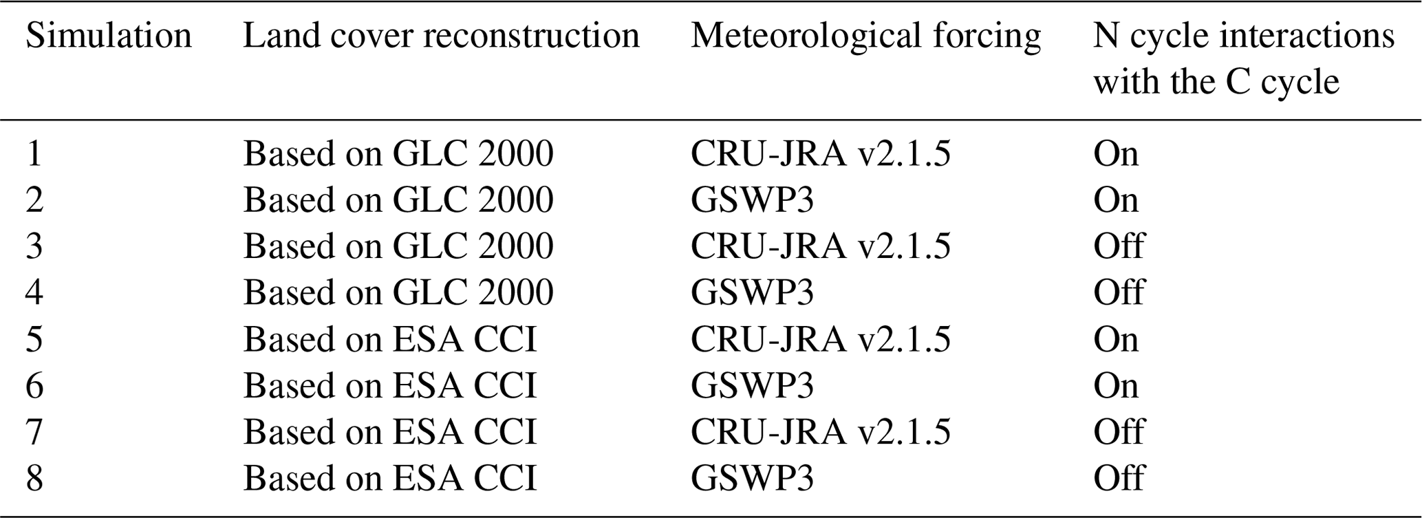
Table 1 Summary of simulations performed with two representations of the historical land cover, two sets of meteorological data, and two versions of the CLASSIC land model.

3.4 Model simulations

Using the two representations of the historical land cover (based on the GLC 2000 and ESA CCI land cover products), the two sets of meteorological data (CRU-JRA and GSWP3), and the two versions of the CLASSIC model (with and without interactions between the C and N cycles), we perform eight sets of pre-industrial and historical simulations, as summarized in Table 1. Pre-industrial simulations that correspond to the year 1700 are required before doing the historical simulations (from which we analyze the model results) so that model pools can be spun up to near equilibrium for each combination of land cover, meteorological forcing, and model version. The pre-industrial simulations use 1901–1925 meteorological data repeatedly, since this period shows few trends in meteorological variables. Global thresholds of net atmosphere–land C flux of 0.05 Pg yr⁻¹ and net atmosphere–land N flux of 0.5 Tg N yr⁻¹ in simulations with the N cycle turned on are used to ensure that the model pools have reached equilibrium. Each historical simulation is then initialized from its corresponding pre-industrial simulation after it has reached equilibrium. Simulations driven with the CRU-JRA meteorological data are performed for the period 1701–2018, and simulations driven with the GSWP3 meteorological data are performed for the period 1701–2016, although results are reported for the period 1997–2016, which is common to both simulations. Similar to the pre-industrial simulations, meteorological data from 1901–1925 are used repeatedly for the period 1701–1900. The global model simulations are performed at a spatial resolution of about 2.81^∘ (about 312 km at the Equator), and the size of the spatial longitude–latitude grid is 128×64 grid cells. All model forcings are regridded to this common spatial resolution. The model is run over about 1900 land grid cells at this resolution, excluding glacial cells in Greenland and Antarctica.

3.5 Automated benchmarking

The results from the eight CLASSIC simulations reported here are evaluated using an in-house model benchmarking system called the Automated Model Benchmarking R package (AMBER; Seiler et al., 2021). AMBER is based on a skill score system originally developed by Collier et al. (2018); this system is used to quantify model performance and is explained in detail in the Appendix. Five scores are used to assess a model's bias (S_bias), root-mean-square error (S_RMSE), seasonality (S_phase), interannual variability (S_iav), and spatial distribution (S_dist) against globally gridded and in situ data set(s) of observation-based estimates for a given quantity. A score is computed by first calculating a dimensionless statistical metric, which is then scaled onto a unit interval, and finally calculating its spatial mean. Scores range from 0 to 1 and are dimensionless. Higher values indicate better performance. Finally, an overall score S_overall is calculated as follows, giving twice as much weight to S_RMSE:

$$\begin{array}{}\text{(1)}& S_{\text{overall}}={\displaystyle \frac{S_{\text{bias}}+\mathrm{2}{S}_{\text{RMSE}}+S_{\text{phase}}+S_{\text{iav}}+S_{\text{dist}}}{\mathrm{1}+\mathrm{2}+\mathrm{1}+\mathrm{1}+\mathrm{1}}}..\end{array}$$

The decision to give extra weight to S_RMSE is entirely subjective but follows Collier et al. (2018).

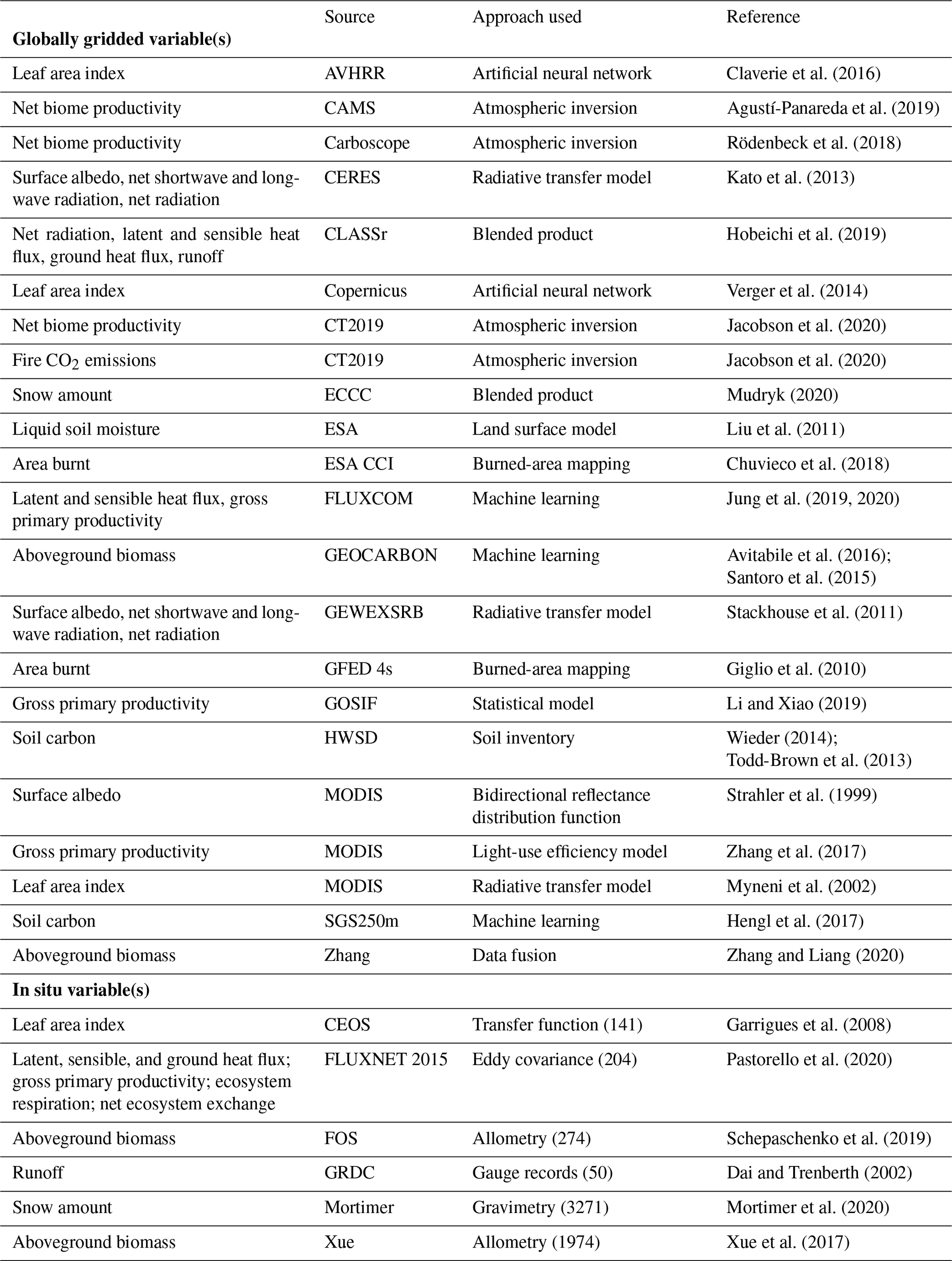
The scores are calculated by comparing gridded and in situ observation-based estimates, referred to as reference data sets in Seiler et al. (2021), for 19 energy- (surface albedo, net shortwave and longwave radiation, total net radiation, latent heat flux, sensible heat flux, and ground heat flux), water- (soil moisture, snow, and runoff), and C-cycle-related(GPP, ecosystem respiration, net ecosystem exchange, net biome productivity, aboveground biomass, soil C, LAI, area burnt, and fire CO₂ emissions) variables to model simulated quantities. Table 2 summarizes the source of these observation-based data sets. The resulting model scores express to what extent simulated and observation-based data agree. A low score does not necessarily indicate poor model performance. Uncertainties in the meteorological forcing data and geophysical fields used to drive the model and/or in the observation-based data itself are possible reasons for the lack of agreement. One way to assess uncertainties in observation-based data sets is to quantify the skill score by comparing two independently derived observation-based data sets (Seiler et al., 2022). The resulting scores are referred to as benchmark scores and quantify the level of agreement among the observation-based data sets themselves, provided, of course, that there are at least two sets of observation-based data for a given quantity. The comparison of model scores against benchmark scores then shows how well a model-simulated quantity compares to the reference data sets relative to the agreement between the observation-based data sets themselves.

Table 2 Observation-based data sets used for model evaluation in AMBER.

4 Results

Figures 2 through 9 show the time series and/or zonally averaged values of annual values of a variable of interest when averaged across four ensemble members each according to whether the N cycle is turned on or not, whether the GLC-2000- or ESA-CCI-based land cover is used, and whether model simulations are driven by the CRU-JRA or GSWP3 meteorological data. Figures A3, A4, A6, A7, A9, and A11 in the Appendix, which are complementary to the above-mentioned figures, show the physical and biogeochemical states of the land surface and primary physical fluxes of water and energy, and primary biogeochemical fluxes of CO₂ simulated by CLASSIC at the land–atmosphere boundary for all eight simulations considered here. While the figures in the Appendix illustrate the range in simulated physical and biogeochemical states and fluxes across the eight simulations, Figures 2 through 9 evaluate the effect of model structure, meteorological forcing, and land cover on a given quantity. We also quantify the spread across the eight simulations in Table 3 using the coefficient of variation (cv = standard deviation/mean) calculated using annual global values for a given quantity averaged over the 1997–2016 20-year period of each simulation. This time period is also used for other reported results.

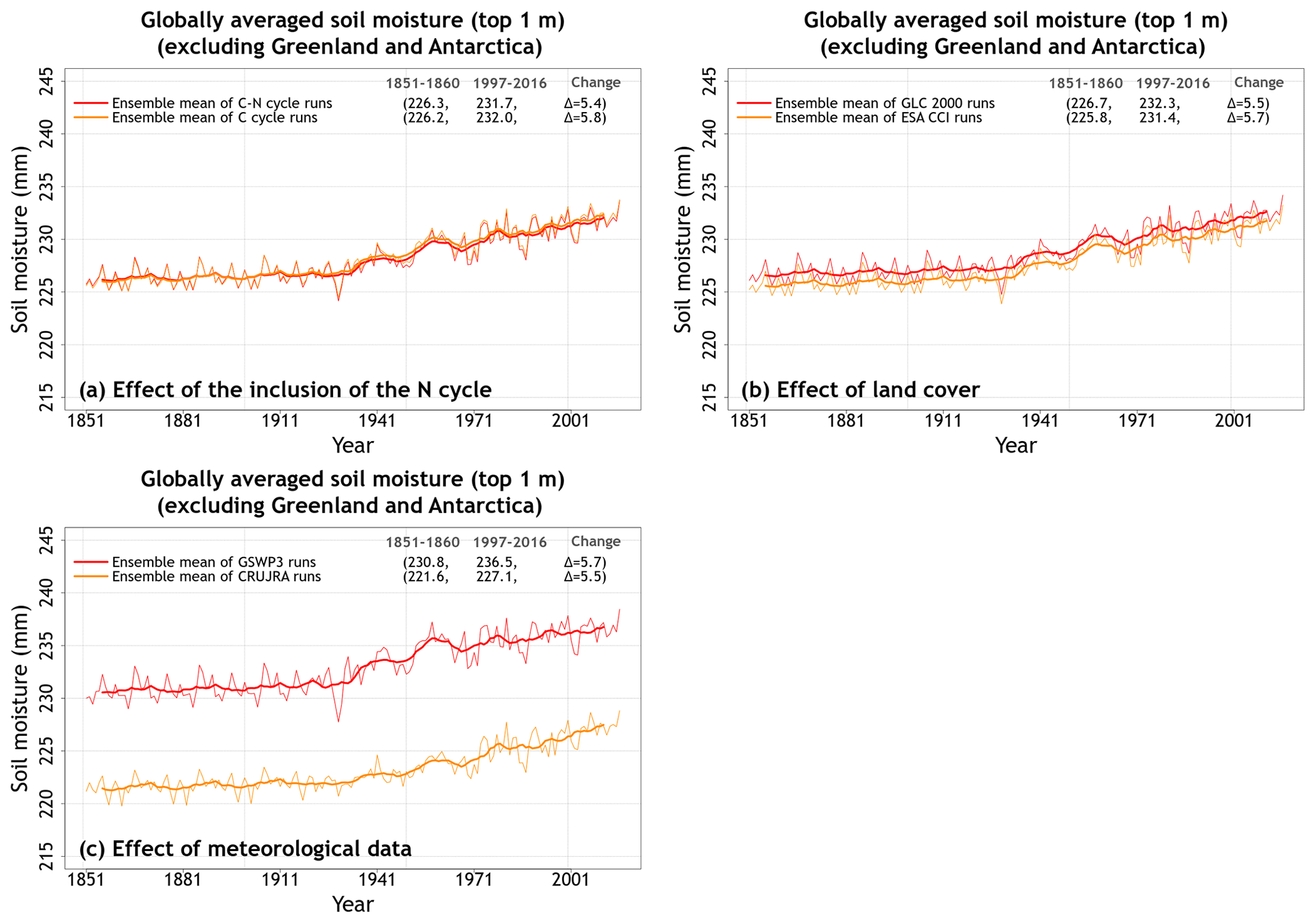
Figure 2 Time series of annual globally averaged soil moisture in the top 1 m averaged over the four ensemble members that are driven with and without an interactive N cycle (a), that are driven with the GLC-2000- and ESA-CCI-based land cover representations (b), and that are driven with the GSWP3 and CRU-JRA meteorological data (c). The thin lines show the individual years, and the thick lines show their 11-year moving average. Model values averaged over the pre-industrial (1851–1860) and present-day (1997–2016) time periods, and their difference, for each ensemble averaged over its set of four simulations are also shown.

4.1 Physical land surface state and fluxes

Figure A3a and b shows the globally averaged simulated soil moisture and temperature in the top 1 m soil layer. While simulated soil temperature in the top 1 m is fairly similar across the eight simulations, the simulated soil moisture is distinctly separated into two groups. The separation into these two groups is caused by the driving meteorological data as shown in Fig. 2. The coefficient of variation for soil moisture and temperature values averaged over the 1997–2016 period of each simulation are 0.02 and 0.004, respectively, indicating that overall the variation in these quantities is relatively small compared to their means. The use of the GSWP3 meteorological data set yields slightly higher (∼4 %) globally averaged soil moisture compared to the CRU-JRA meteorological data set (236.5 mm vs. 227.1 mm; Fig. 2c) for the 1997–2016 period.

Figure A3c and d shows the simulated fluxes of global evapotranspiration and runoff across the eight simulations. Similarly to soil moisture, evapotranspiration and runoff also fall broadly into two groups, and the reason for this is again the driving meteorological data. Figure 3 shows that, while the biggest factor that affects evapotranspiration and runoff is the difference in driving meteorological data, the interactive N cycle also affects these water fluxes. Neither evapotranspiration nor runoff is significantly affected by the choice of land cover. The reason an interactive N cycle affects evapotranspiration is that the N cycle in CLASSIC affects the rate of photosynthesis through the prognostic determination of leaf N content. Photosynthesis in turn affects canopy conductance, which affects transpiration through the canopy leaves. Average evapotranspiration over the 1997–2016 period of the simulations driven with GSWP3 meteorological data is about 9 % lower than in simulations driven with CRU-JRA meteorological data (65.8 vs. 72.1×1000 km³ yr¹; Fig. 3e). An interactive N cycle reduces evapotranspiration by about 2 % due to lower photosynthesis rates, as shown later (Fig. 3a). Average runoff is about 27 % higher in simulations driven with GSWP3 compared to simulations driven with CRU-JRA meteorological data (52.6 vs 41.3×1000 km yr¹; Fig. 3f). This is due to slightly high precipitation in the GSWP3 meteorological data set (Fig. A1) but is more so due to the simulated lower evapotranspiration when using the GSWP3 data (Fig. 3e). The coefficient of variation for evapotranspiration and runoff values averaged over the last 20 years of each simulation are 0.05 and 0.13, respectively.

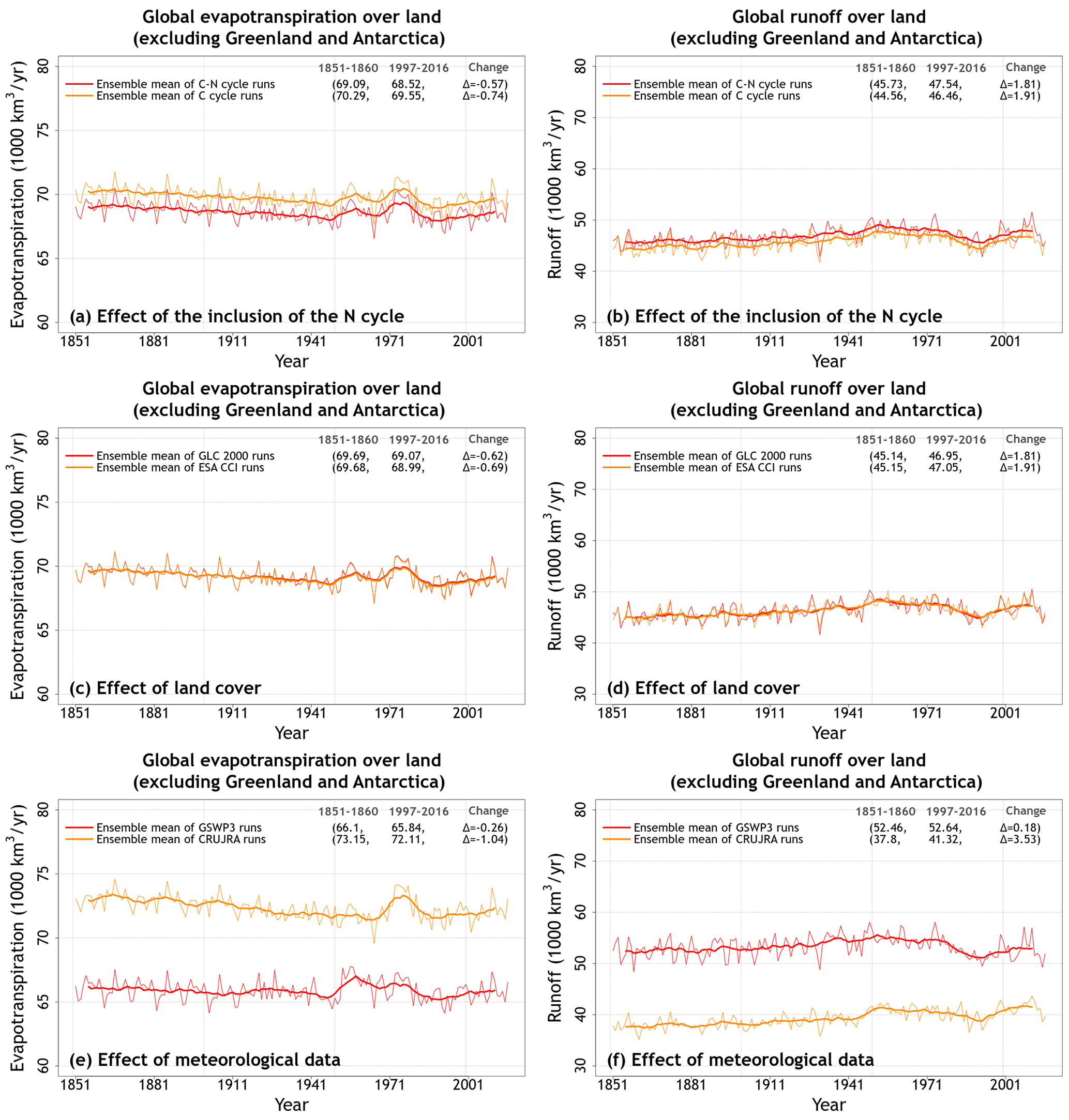
Figure 3 Time series of annual global evapotranspiration and runoff (over all land area excluding Greenland and Antarctica) averaged over the four ensemble members that are driven with and without an interactive N cycle (a, b), that are driven with the GLC-2000- and ESA-CCI-based land cover  (c, d), and that are driven with the GSWP3 and CRU-JRA meteorological data (e, f). The thin lines show the individual years, and the thick lines show their 11-year moving average. Model values averaged over the pre-industrial (1851–1860) and present-day (1997–2016) time periods, and their difference, for each ensemble averaged over its set of four simulations are also shown.

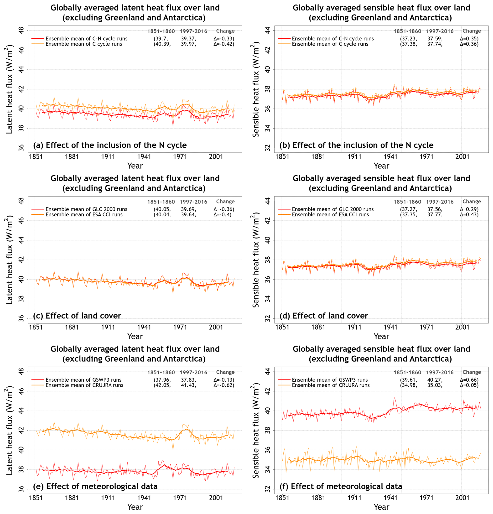
Figure 4 Time series of annual global latent and sensible heat fluxes (over all land area excluding Greenland and Antarctica) averaged over the four ensemble members that are driven with and without an interactive N cycle (a, b), that are driven with the GLC-2000- and ESA-CCI-based land cover (c, d), and that are driven with GSWP3 and CRU-JRA meteorological data (e, f). The thin lines show the individual years, and the thick lines show their 11-year moving average. Model values averaged over the pre-industrial (1851–1860) and present-day (1997–2016) time periods, and their difference, for each ensemble averaged over its set of four simulations are also shown.

Figure A4 shows the primary energy fluxes from the eight simulations. These include net downward shortwave and longwave radiation and latent and sensible heat fluxes. Incoming shortwave and longwave radiation are part of the driving meteorological data. Similarly to water fluxes, the differences in energy fluxes in CLASSIC are also primarily driven by differences in meteorological data (Figs. A4, A5, and 4). Net shortwave radiation (Fig. A4a) is equal to incoming shortwave radiation minus the fraction that is reflected back. Net longwave radiation (Fig. A4b) is equal to incoming longwave radiation minus the longwave radiation emitted by the land based on its surface temperature following the Stefan–Boltzmann law. The difference in net shortwave radiation is also affected by simulated vegetation biomass and leaf area index. The latter affects surface albedo, which determines what fraction of incoming shortwave radiation is reflected. This is the reason why an interactive N cycle affects net shortwave radiation, since the N cycle affects photosynthesis and, in turn, simulated vegetation biomass and leaf area index (Fig. A5b). Latent heat flux is affected primarily by meteorological data (Fig. 4) but also by whether the N cycle is interactive or not, since it is essentially evapotranspiration but in energy units. Finally, differences in sensible heat fluxes are strongly affected by differences in driving meteorological data (Fig. 4). Globally averaged sensible heat flux in the simulations driven with GSWP3 data is ∼14 % higher compared to CRU-JRA-driven simulations (40.2 vs. 35.0 W m⁻²). The coefficients of variation for latent and sensible heat flux values averaged over the last 20 years of each simulation are 0.05 and 0.07, respectively. Net shortwave (cv = 0.006) and longwave (cv = 0.03) radiative fluxes vary little across the eight simulations.

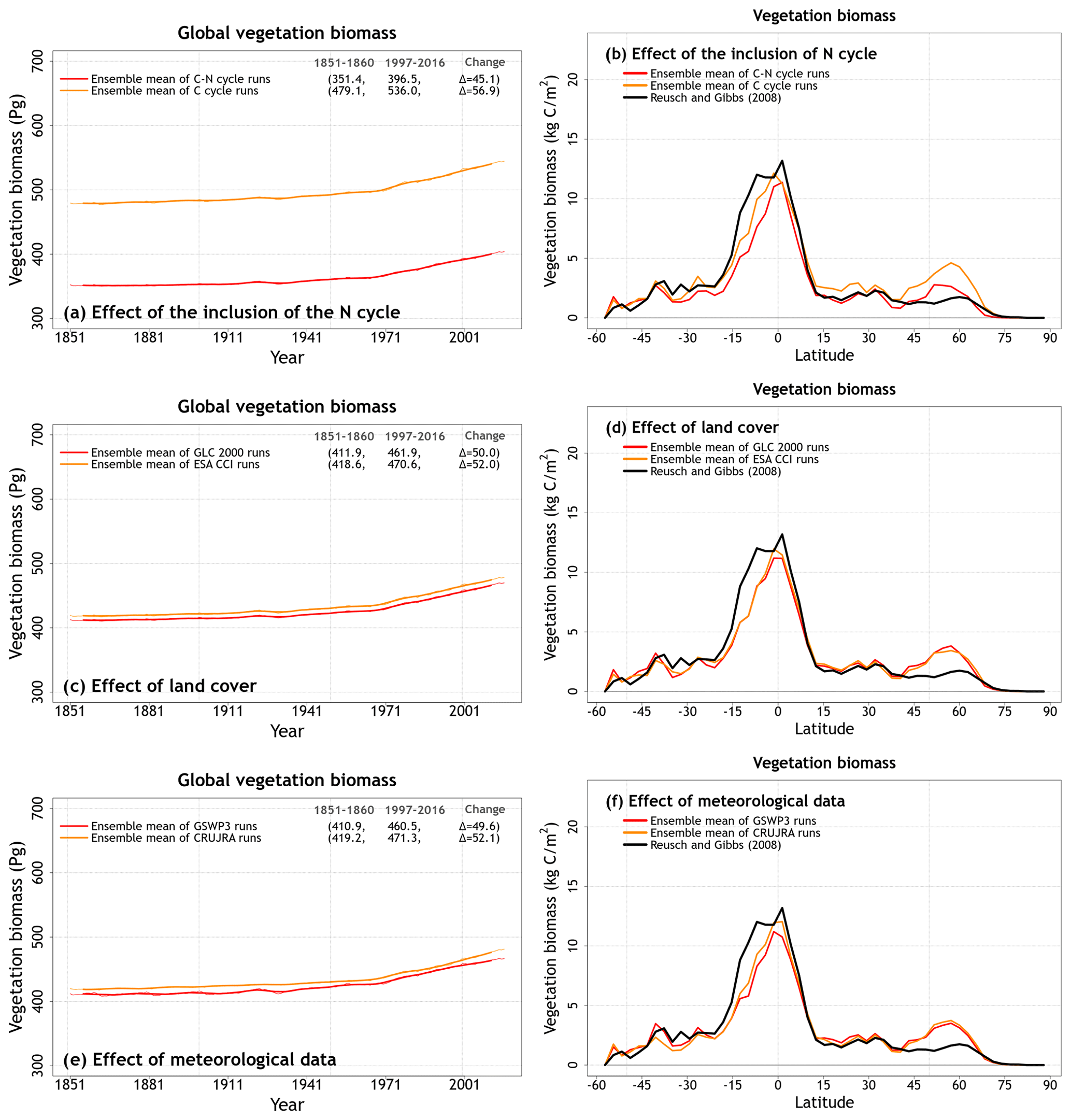
Figure 5 Time series of annual global vegetation C mass (over all land area excluding Greenland and Antarctica) (a, c, e) and zonally averaged values of vegetation C mass over land (b, d, f) averaged, for the period 1997–2016, over the four ensemble members that are driven with and without an interactive N cycle (a, b), that are driven with the GLC-2000- and ESA-CCI-based land cover (c, d), and that are driven with GSWP3 and CRU-JRA meteorological data (e, f). The thin lines for the time series show the individual years, and the thick lines show their 11-year moving average. Model values averaged over the pre-industrial (1851–1860) and present-day (1997–2016) time periods, and their difference, are also shown in (a, c) and (e).

4.2 Biogeochemical land surface state and fluxes

4.2.1 Primary CO₂ fluxes and C pools

Figure A6 shows the simulated C state of the land surface expressed in terms of vegetation and soil C pools. Panels a and b show the annual time series of global vegetation and soil C mass from the eight simulations, and panels c and d show their zonally averaged distributions averaged over the last 20 years of each simulation. The biggest difference in the time series of global vegetation (cv = 0.16) and soil (cv = 0.21) C mass compared to soil moisture and temperature, which characterized the physical land surface state, is the large spread across the eight simulations, as indicated by their high cv values. The zonally averaged values further provide insight into the reasons for this spread and show that the largest differences between simulated vegetation and soil C occur at northern high latitudes (north of about 40^∘ N). Figure A6c, d also show observation-based zonally averaged values of vegetation and soil C mass based on Reusch and Gibbs (2008) and the Harmonized World Soil Database (v1.2; Fischer et al., 2008), respectively, to provide a reference. A more thorough comparison with observations is provided in Sect. 4.3.

Differences in vegetation C mass are dependent primarily on whether the N cycle is interactive or not. (Fig. 5). Both land cover and the driving meteorological data play a smaller role in the simulated spread of vegetation C mass (Fig. 5). The ESA-CCI-based land cover has a larger vegetated area, but most of this increase comes from an increase in the area of grasses that do not store a lot of C in their vegetation C mass. The spread in simulated soil C is due to the N cycle but also the choice of land cover (Fig. 6). Since CLASSIC assumes that litter from grasses is more recalcitrant than that from trees, the choice of ESA-CCI-based land cover leads to a higher soil C mass because it has a higher grass area than the GLC-2000-based land cover (Fig. 6c, d). The choice of meteorological data does not affect the magnitude of simulated globally summed soil C mass significantly but does affect its change over the historical period. In Fig. 6c, the decrease in soil C mass from the 1851–1860 period to the 1997–2016 period is higher when using the GSWP3 (29.9 Pg C) compared to when using the CRU-JRA (14.8 Pg C) meteorological data.

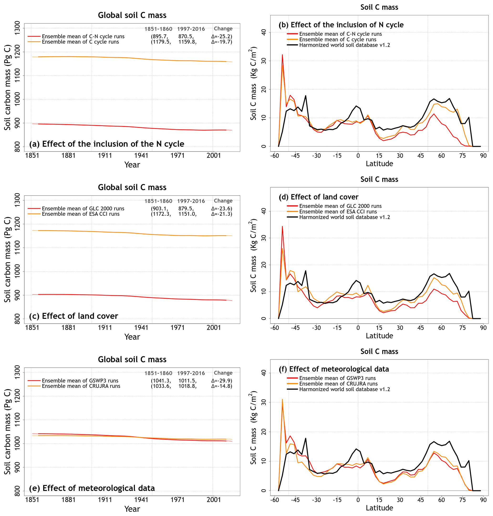
Figure 6 Time series of annual global soil carbon mass (over all land area excluding Greenland and Antarctica) (a, c, e) and zonally averaged values of soil carbon mass over land (b, d, f) averaged, for the period 1997–2016, over the four ensemble members that are driven with and without an interactive N cycle (a, b), that are driven with the GLC-2000- and ESA-CCI-based land cover representations (c, d), and that are driven with GSWP3 and CRU-JRA meteorological data (e, f). The thin lines for the time series show the individual years, and the thick lines show their 11-year moving average. Model values averaged over the pre-industrial (1851–1860) and present-day (1997–2016) time periods, and their difference, are also shown in (a, c, e).

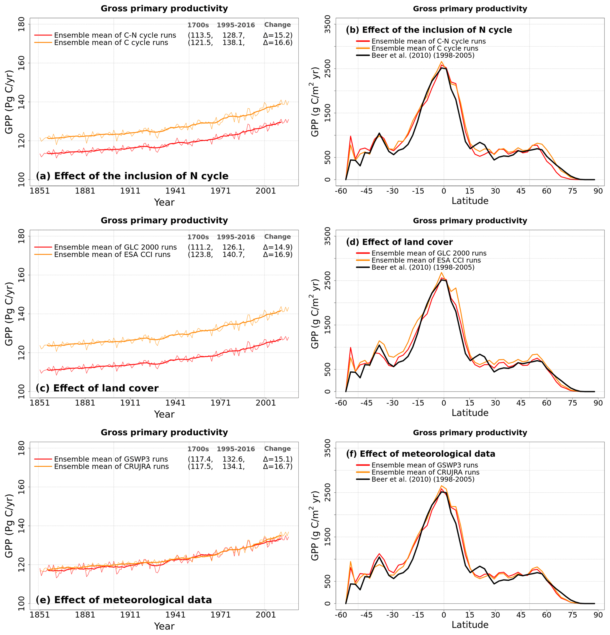
Figure 7 Time series of annual global gross primary productivity (over all land area excluding Greenland and Antarctica) (a, c, e) and zonally averaged values of gross primary productivity over land (b, d, f) averaged, for the period 1997–2016, over the four ensemble members that are driven with and without an interactive N cycle (a, b), that are driven with the GLC 2000 and ESA CCI based land cover representations (c, d), and that are driven with GSWP3 and CRU-JRA meteorological data (e, f). The thin lines for the time series show the individual years, and the thick lines show their 11-year moving average. Model values averaged over the pre-industrial (1851–1860) and present-day (1997–2016) time periods, and their difference, are also shown in a, c, e.

The reason why an interactive N cycle in CLASSIC affects vegetation C and soil C mass, and why the ESA-CCI-based land cover yields high soil C, is seen in Figs. A7 and 7. Figure A7 in the Appendix shows the spread of primary C fluxes, including gross primary productivity (GPP; cv = 0.07) and autotrophic (cv = 0.04) and heterotrophic (cv = 0.10) respiratory fluxes, across the eight simulations. Since GPP is lower in the runs with the N cycle, both vegetation (Figure 5a) and soil C mass (Fig. 6a) are also lower. The lower GPP in the runs with the N cycle is due primarily to lower GPP at high latitudes (Fig. 7b), which yields low vegetation C mass at high latitudes (Fig. 5b). Low GPP at high latitudes translates to even larger relative differences in soil C given the longer turnover timescales of soil C at high latitudes (Fig. 6b). The use of the ESA-CCI-based land cover, which has a higher grass area than the GLC-2000-based land cover, leads to higher GPP (Fig. 7d) and therefore higher soil C at all latitudes (Fig. 6d). In Fig. A8 in the Appendix, global heterotrophic and autotrophic respiratory fluxes are most affected by land cover and the inclusion or absence of an interactive N cycle but not as much by the driving meteorological data.

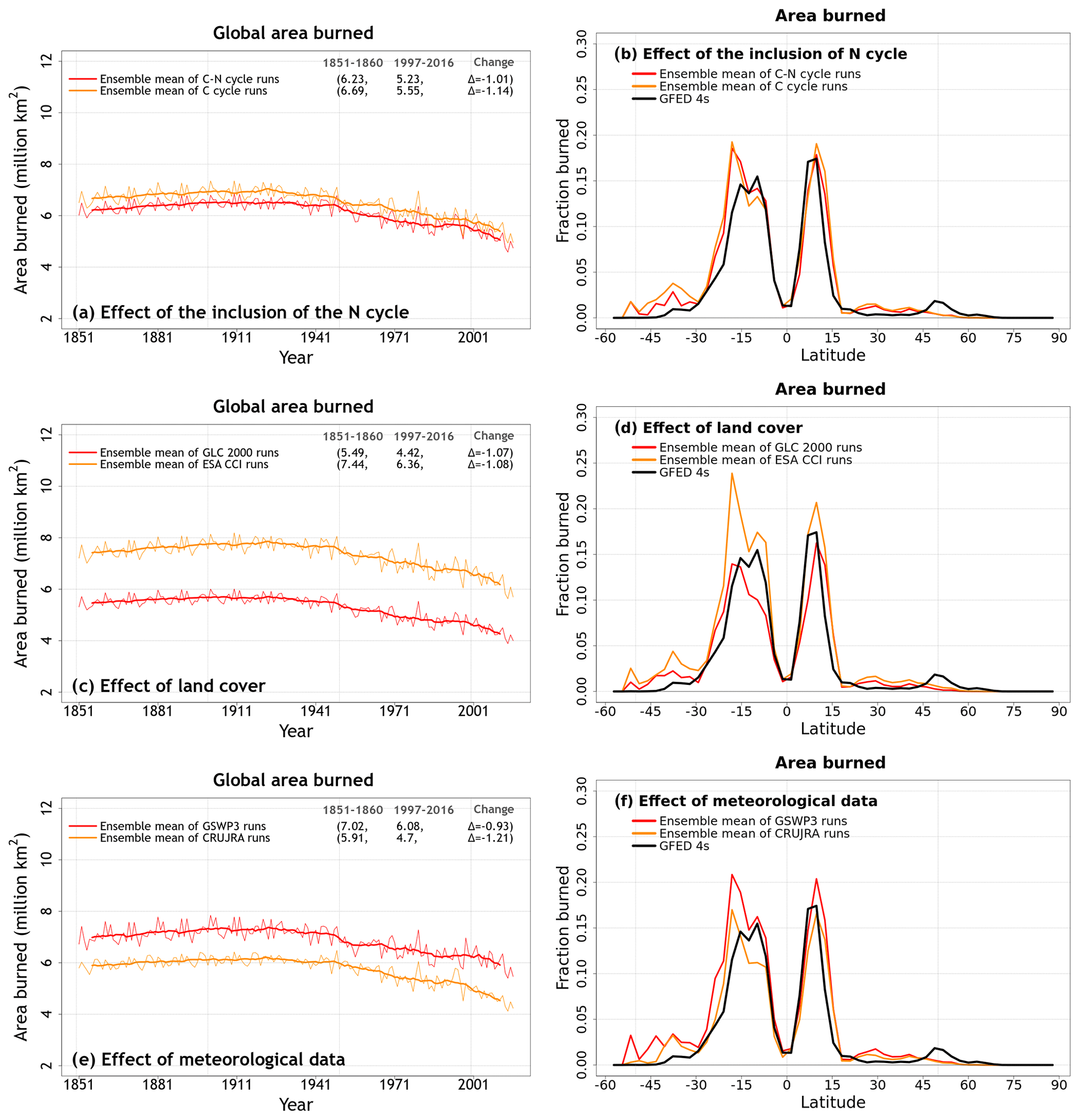
Figure 8 Time series of annual area burned (over all land area excluding Greenland and Antarctica) (a, c, e) and zonally averaged values of area burned (d, e, f) averaged, for the period 1997–2016, over the four ensemble members that are driven with and without an interactive N cycle (a, b), that are driven with the GLC 2000 and ESA CCI based land cover representations (c, d), and that are driven with GSWP3 and CRU-JRA meteorological data (e, f). The thin lines for the time series show the individual years, and the thick lines show their 11-year moving average in (a, c, e). Model values averaged over the pre-industrial (1851–1860) and present-day (1997–2016) time periods, and their difference, are also shown for (a), (c), and (e).

The transient behaviour of heterotrophic respiration over the historical period is not affected by meteorological data, although the effect of meteorological data on autotrophic respiration varies over time.

4.2.2 Area burned and fire CO₂ emissions

Figure A9 shows the time series of global area burned and global fire CO₂ emissions and their zonally averaged values. We chose the area burned (cv = 0.24) and fire CO₂ emissions (cv = 0.21) in addition to the primary biogeochemical fluxes because fire shows large variability both in space and in time and because both these variables yield the largest spread across the eight simulations among all the fluxes and simulated quantities considered here. Figure A9 (panels c and d) in the Appendix also shows observation-based estimates for area burned and fire CO₂ emissions based on GFED 4s (Giglio et al., 2013) to provide an observation-based context. Figures 8 and A10 help us understand which factors contribute to this large variability. The variability in the area burned is caused primarily by the choice of land cover and meteorological data, and the variability is higher in the Southern Hemisphere (Fig. 8d, f). An interactive N cycle does not affect the zonal distribution of area burned and fire CO₂ emissions (Figs. 8 and A10) as much. The reason both area burned and fire CO₂ emissions are affected by the choice of land cover is because the ESA CCI land cover has higher grass area, and as a result, it yields higher area burned and fire CO₂ emissions, since a larger area is burned for grasses than for trees in the model. The choice of driving meteorological data is a factor in the area burned, and our simulations show that the use of GSWP3 meteorological forcing yields a higher area burned than the CRU-JRA data. In particular, wind speed, which determines the rate of spread of fire in CLASSIC, is much higher in the GWSP3 than in the CRU-JRA meteorological data. Globally averaged land wind speed (excluding Greenland and Antarctica) in GSWP3 data is 6.1 m s⁻¹ compared to 3.4 m s⁻¹ in the CRU-JRA data for the period 2000–2016.

Table 3 Simulated energy, water, and carbon cycle quantities considered in this study sorted according to their coefficient of variation. The quantities are listed from the most variable at the top to the least variable at the bottom. The coefficient of variation is based on annual values averaged over the 1997–2016 period across the eight simulations. The last column shows the dominant source of variability for each model-simulated quantity.

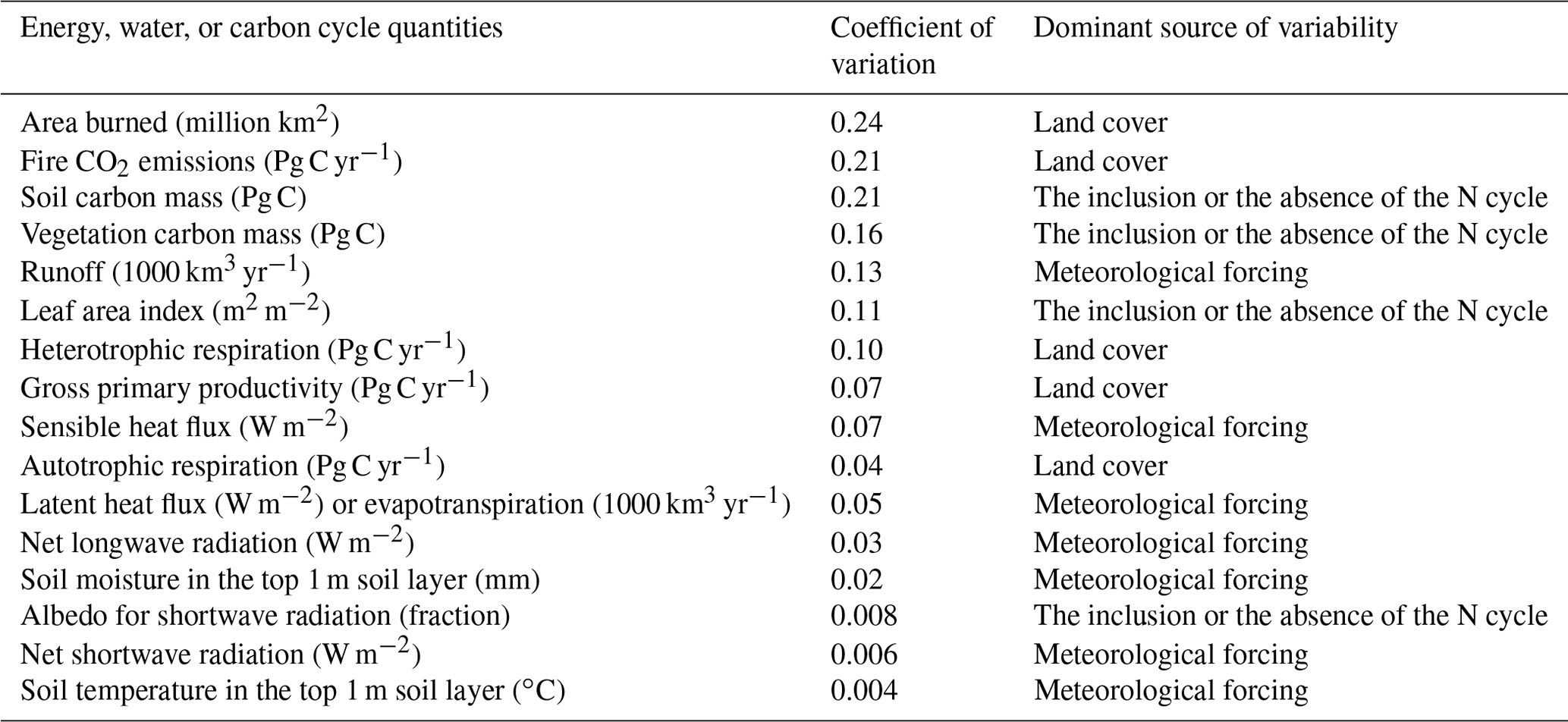
4.2.3 Coefficient of variation summary

Table 3 shows the energy, water, and C-related quantities considered so far, as well as leaf area index and albedo, and lists them from the most variable at the top to the least variable at the bottom according to their coefficient of variation. The area burned is found to be the most variable quantity, and soil temperature is the least variable quantity. Table 3 also shows the most dominant source of variability for each simulated quantity: land cover, meteorological forcing, or the inclusion or absence of an interactive N cycle. Net atmosphere–land CO₂ flux (or net biome productivity), net ecosystem exchange, and ground heat flux are not included in Table 3 because these fluxes are calculated as the difference of larger fluxes, and as a result, their values are closer to zero, which yields a large value of the coefficient of variation. Net surface radiation is the sum of net shortwave and longwave radiation, and both of them exhibit a low coefficient of variability across the eight simulations (Table 3).

4.2.4 Model tuning

Overall, the results presented so far illustrate that different model-simulated quantities are sensitive to different forcings and model versions. The use of more than one meteorological forcing data set and land cover representation and the use of two model versions (with and without N cycle) yields a dilemma, since it is no longer possible to tune model parameters without choosing a preferred meteorological data set, land cover representation, and model version. As such, it seems logical that, rather than tuning the model for a preferred forcing or model version, model results from an ensemble of simulations should be compared against an ensemble of observations in so far as it is possible. This is the approach taken in Sect. 4.3 with automated benchmarking.

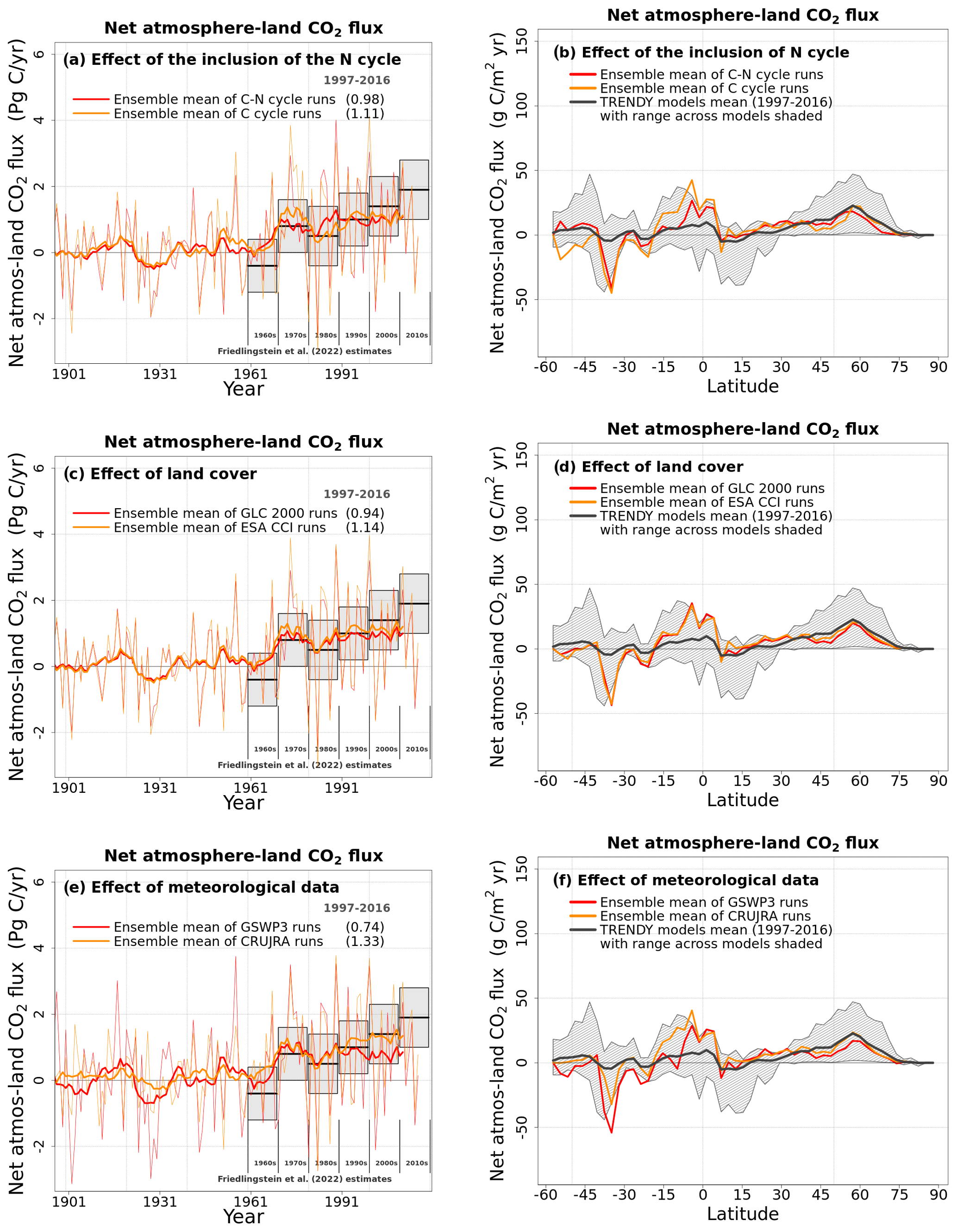
Figure 9 Time series of global net atmosphere–land CO₂ flux (over all land area excluding Greenland and Antarctica) (a, c, e) and its zonally averaged values (b, d, f) averaged, for the period 1997–2016, over the four ensemble members that are driven with and without an interactive N cycle (a, b), that are driven with the GLC-2000- and ESA-CCI-based land cover representations (c, d), and that are driven with GSWP3 and CRU-JRA meteorological data (e, f). The thin lines for the time series show the individual years, and the thick lines show their 11-year moving average. Model values averaged over the pre-industrial (1851–1860) and present-day (1997–2016) time periods, and their difference, are also shown for panels (a), (c), and (e).

4.2.5 Net biome productivity

Figure A11 shows the spread in the time series of annual global net atmosphere–land CO₂ flux and their zonally averaged values across the eight simulations averaged over the 1997–2016 period from each simulation. The global net atmosphere–land CO₂ flux or net biome productivity (NBP) is considered to be a critical determinant of the performance of LSMs and is treated as such by TRENDY because this flux ultimately affects the changes in the atmospheric CO₂ burden. TRENDY requires that LSMs simulate a terrestrial C sink for the decades of the 1990s to the present to be considered for inclusion in the TRENDY ensemble.

Figure A11 in the Appendix also shows the estimates of global net atmosphere–land CO₂ flux from the participating TRENDY models in grey boxes, with mean and shaded ranges for the decades from the 1960s to 2010s from the Global Carbon Project (Friedlingstein et al., 2022). Positive values in Fig. A11 indicate a C sink over land, and negative values indicate a C source to the atmosphere. In Fig. A11a, all eight simulations reported here would qualify for inclusion in the TRENDY ensemble, since they all simulate a terrestrial C sink from the 1990s to the present day. Before 1960, since the atmospheric CO₂ concentration is not high enough, the model yields both a land C sink and source in response to interannual variability in meteorological data. In addition, the time series of global NBP from all eight simulations lie within the uncertainty range of reported estimates from the Global Carbon Project. Figure A11a suggests that, based on global NBP, at least, it is not possible to exclude any of the eight simulations. In Fig. A11b, zonally averaged NBP averaged over the 1997–2016 period from each of the eight simulations mostly lie within the range of NBP simulated by models that participated in TRENDY 2020. CLASSIC simulates a C sink at northern high latitudes consistent with TRENDY models, but it simulates a C sink on the stronger side of TRENDY models in the southern tropics (0–20^∘ S). This is likely because CLASSIC is known to simulate low C emissions associated with LUCs, most of which are generated in tropical regions (Asaadi and Arora, 2021).

Figure 9 provides additional insights into the effect of different forcings on the simulated NBP. In Figure 9, averaged over the 1997–2016 period, an interactive N cycle leads to a somewhat weaker C sink (panel a: 0.98 vs. 1.11 Pg C yr⁻¹), the choice of the ESA-CCI-based land cover leads to a somewhat stronger C sink (panel c: 1.14 vs 0.94 Pg C yr⁻¹), and the choice of the GSWP3 meteorological data leads to a much weaker C sink (panel e: 0.74 vs 1.33 Pg C yr⁻¹) than the CRU-JRA meteorological data. In Figure 9a, b, the largest difference between the model versions with and without the N cycle occurs in the tropics (∼5^∘ N–20^∘ S), where an interactive N cycle leads to a weaker C sink. There are differences in zonally averaged NBP with and without the N cycle south of 45^∘ S, but the land area below this latitude is small, so the averages are calculated over only a few grid cells. The choice of the land cover (Fig. 9c, d) does not substantially change the distribution of the zonally averaged values of NBP, although, as noted above, the choice of ESA-CCI-based land cover leads to a somewhat stronger C sink. Finally, the choice of the GSWP3 meteorological forcing leads to a weaker C sink at most latitudes (Fig. 9e, f).

4.3 Automated benchmarking

Figure 10 plots the overall score, S_overall, against benchmark scores for 16 of the 19 energy-, water-, and C-cycle-related variables using AMBER-calculated model and benchmark scores. AMBER does not yet evaluate N-cycle-related variables, for which observations are more scarce than for C-cycle-related variables. The range in model scores comes from the eight simulations, and the range in benchmark scores comes from the different observation-based data sets. The whiskers show the range in the overall score both for the benchmark and model scores. The vertical whiskers show the range of eight model scores when a given variable from all eight model simulations is compared to an observation-based data set. The horizontal whiskers show the range when three or more observation-based data sets are compared to each other. When only two observation-based data sets are compared to each other, there is only one benchmark score, and therefore there is no range. In Fig. 10, three quantities are missing: soil moisture, ecosystem respiration, and fire CO₂ emissions, since there is only one observation-based reference data set available for these variables; therefore, a benchmark score cannot be calculated. Figure 10 shows that, typically, as the benchmark scores increase, so do the overall model scores for a given quantity. This indicates that uncertainty in observation-based estimates themselves leads to a poor agreement between observations and model-simulated quantities.

For energy and water flux scores (panels a and b), the model overall scores lie around the 1:1 line, indicating that model scores are generally as good as the benchmark scores, except in the case of surface albedo (ALBS), runoff (MRRO), ground heat flux (HFG), and comparison against one observation-based estimate of snow water equivalent, all of which lie below the 1:1 line. For C-cycle-related variables, most scores lie somewhat below the 1:1 line, indicating that simulated quantities do not agree as well with observations as observations agree among themselves. The lower benchmark score for soil C (panel c) is because the SoilGrids250m (SG250m) data and the Harmonized World Soil Database (HWSD) do not agree well amongst themselves because the SG250m soil C data include peatlands and permafrost C at high latitudes, while the HWSD data do not (see Fig. 11b). Since the version of CLASSIC used here does not represent peatlands and permafrost C, it compares better with the HWSD data than with the SG250m data. In the case of soil C, the choice of HSWD data for comparison against model values is obvious. However, for other variables, it may not always be obvious which observation-based estimate is more appropriate or better for comparison against model results. The uncertainty in forcing data sets and in observation-based estimates, against which model results are evaluated, implies that even a perfect model cannot be evaluated to its fullest extent.

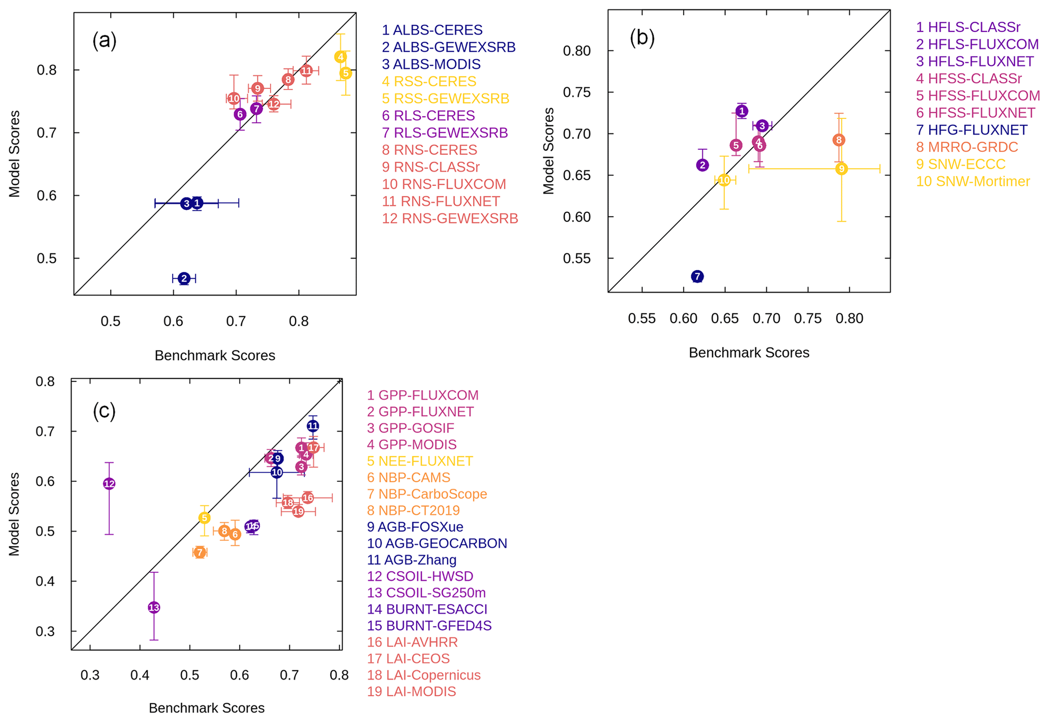
Figure 10 Comparison of benchmark scores with model overall scores for a range of energy-, water-, and carbon-related quantities. The whiskers indicate the range for benchmark scores across different observation-based data sets and the range across the eight model simulations for the overall model scores. The quantities in (a) are ALBS (surface albedo), RSS (net shortwave radiation), RLS (net longwave radiation), and RNS (net radiation). Quantities in (b) are HFLS (latent heat flux), HFSS (sensible heat flux), HFG (ground heat flux), MRRO (runoff), and SNW (snow water equivalent). Quantities in (c) are GPP (gross primary productivity), NEE (net ecosystem exchange), NBP (net biome productivity), AGB (aboveground biomass), CSOIL (soil carbon mass), BURNT (area burned), and LAI (leaf area index).

Figure 11 shows the zonal distribution of vegetation C mass, LAI, area burnt, GPP, and fire CO₂ emissions (which constitute standard output from AMBER) and illustrates how AMBER compares the spread across the simulations, indicated by 50 %, 80 %, and 100 % shading against observation-based estimates. The black and shades of grey indicate the model mean and the spread across the eight model simulations, respectively, and the thick lines in other colours show the mean values of observation-based estimates. The time period over which observations and model quantities are averaged is chosen to be the same. In Figure 11a, for aboveground biomass, the GEOCARBON data set uses one product for the extratropics and another for the tropics to create a global aboveground-biomass product. The Zhang product (Zhang and Liang, 2020) is based on the fusion of multiple gridded biomass data sets for generating a global product. Both products are described in detail in Seiler et al. (2022). The model results generally compare better with the Zhang product outside the 10^∘ N to 10^∘ S region, but they compare better with the GEOCARBON product within this region. The values to the south of 40^∘ S are generally less reliable because of the little vegetated land area below this latitude. In Fig. 11b, the model-simulated values for soil organic C compare better with the HWSD data set compared to the SG250m data for reasons mentioned in the previous paragraph. Simulated leaf area index (Fig. 11c) and gross primary productivity (Fig. 11e) generally compare well in terms of their observation-based estimates. The simulated area burned (Fig. 11d) and fire emissions (Fig. 11f) also compare well with observation-based estimates except that the model is not able to capture the small area burned and emissions at northern high latitudes between around 50 to 70^∘ N. Figures A12 and A13 in the Appendix compare zonally averaged values of other simulated quantities with observation-based estimates used in the AMBER framework. Together, Figs. 11, A12, and A13 illustrate that the model is overall able to capture the latitudinal distribution of most land surface quantities.

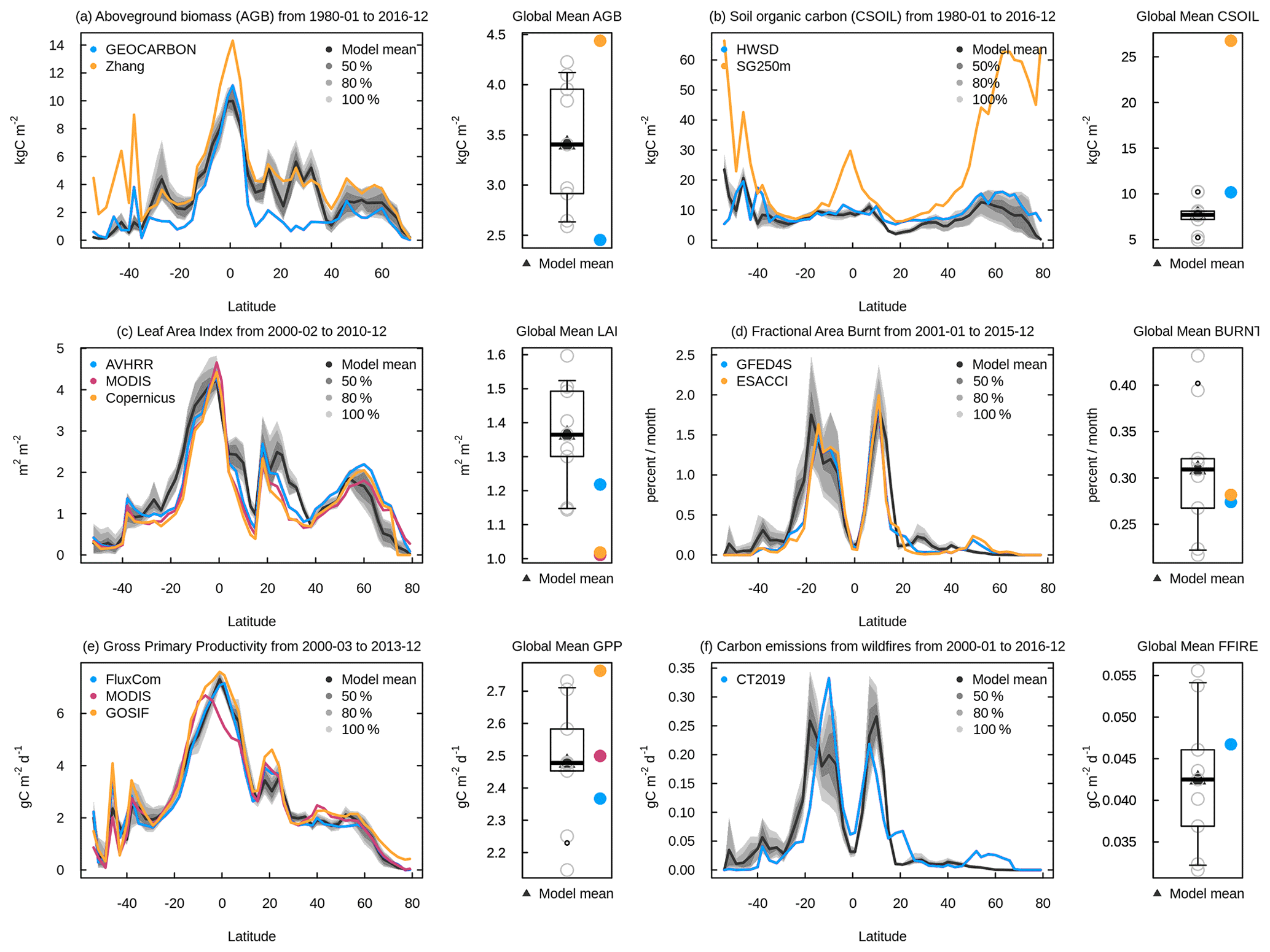
Figure 11 Zonally averaged values of aboveground biomass (a), soil carbon mass (b), leaf area index (c), fractional area burnt (d), gross primary productivity (e), and fire CO₂ emissions (f) from the eight simulations summarized in Table 1. The model results are shown as their mean (black) and as the spread across the eight simulations, indicated by 50 %, 80 %, and 100 % ranges in different shades of grey. The observation-based estimates used in AMBER to calculate scores are shown in coloured lines.

Since overall scores are available for all eight simulations for model quantities that are compared to observations, it is possible to evaluate how an interactive N cycle and the choice of meteorological data and land cover data affect model performance. Figure 12 summarizes the differences in overall scores for model quantities and combinations for which the differences are statistically significant at the 5 % level based on Tukey's test (Beyer, 1981). The score indicated in parentheses for each quantity is the average score across the eight simulations and provides context. For example, when evaluating the effect of change in land cover for NEE, the use of the GLC-2000-based land cover, compared to the use of the ESA-CCI-based land cover, degrades the average score for net ecosystem exchange by about 0.02 given that the average score for net ecosystem exchange is 0.53. The error bars on the value 0.02 denote the 95 % confidence interval and in this case are calculated by differencing four simulations that use the GLC-2000-based land cover and four simulations that use the ESA-CCI-based land cover. The use of the GLC-2000-based land cover, on the other hand, slightly improves scores for ecosystem respiration and liquid soil moisture. The use of GSWP3 data improves model scores for net shortwave, longwave, and total radiation and for sensible and ground heat flux but degrades the overall score for area burned and soil moisture and more so for snow water equivalent. Finally, an interactive N cycle slightly improves model performance for area burned and fire CO₂ emissions (due to improved aboveground biomass in the tropics) but degrades it for ecosystem respiration, GPP, and net ecosystem exchange. The inclusion of an interactive N cycle changes V_c,max to a prognostic variable for each PFT as opposed to being specified based on observations. This is analogous to running an atmospheric model with a fully dynamic three-dimensional ocean as opposed to using specified sea surface temperatures (SSTs) and sea ice concentrations (SICs). Using a dynamic ocean allows future projections (since future SSTs and SICs are not known) but invariably degrades a model's performance for the present day, since simulated SSTs and SICs will have their biases. Similarly, using an interactive N cycle allows future changes in V_c,max (based on changes in N availability) to be projected but also degrades CLASSIC's performance for the present day, since simulated V_c,max has its own biases. Overall, the model performance is most affected by the choice of the driving meteorological data for water and energy fluxes and by the inclusion or absence of an N cycle and by the choice of land cover for carbon-cycle-related state variables and fluxes.

5 Conclusions

The response of the terrestrial biosphere over the historical period is driven primarily by four global change drivers – increasing atmospheric CO₂, changing climate, LUC, and N deposition and fertilizer application. Our framework allows us to evaluate how a land surface model responds to increasing atmospheric CO₂, changing climate, and anthropogenic N additions to the coupled soil–vegetation system and how this response is dependent on two driving meteorological data sets, two land cover representations, and the two model variations (with and without an interactive N cycle). However, the framework used here does not quantify the uncertainty associated with LUC over the historical period, since we use only one reconstruction of increasing crop area over the historical period. These results help draw three primary conclusions. First, even if the observations and models were perfect (including their structure and their parameterizations), the uncertainty associated with driving meteorological data and geophysical fields makes it difficult to evaluate LSMs. The uncertainty in global-scale driving data implies that a model can never be truly evaluated to its fullest extent. Model results can only be as good as the data that are used to force them, and therefore, even a perfect model cannot yield perfect results.

Second, model tuning when driving the model with a single set of forcings and evaluating it against a single set of observations is likely not a fruitful exercise. Models should not be tuned to a single set of driving data and observation-based evaluation data. Rather, their performance must be evaluated against a range of available observations in light of the uncertainty associated with driving data and the uncertainty associated with observations. A model's ability to reproduce a given single set of observations when driven with a single set of driving data is not a true measure of its success. Here again, a perfect model driven by perfect forcing data cannot be truly evaluated to its fullest extent, since observations themselves have uncertainties.

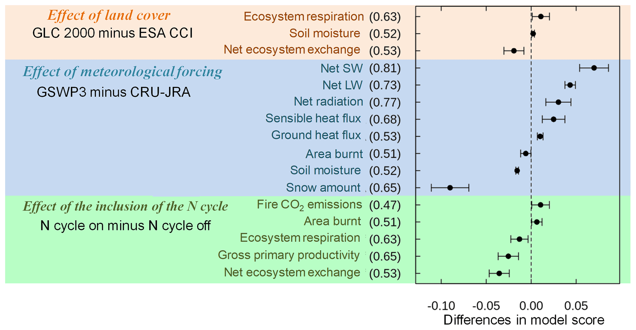
Figure 12 Summary of differences in overall scores for model-simulated quantities and combinations for which the differences are statistically significant. The scores in parentheses for each quantity are the average scores across the eight simulations and provide context. The error bars denote the 95 % confidence interval, as explained in the text.

Third, with the caveat that our framework uses only one reconstruction of increase in crop area over the historical period, the response of a model expressed in terms of net atmosphere–land CO₂ flux to perturbation in meteorological, CO₂, and LUC forcing over the historical period appears to be largely independent of its pre-industrial state as simulated here. The pre-industrial soil and vegetation C masses for the eight simulations considered here vary between 1035 ± 195 and 405 ± 58 Pg C (mean ± standard deviation), respectively. Both pre-industrial and present-day vegetation and soil C pools explain only about 2 % to 7 % of the variability in simulated net atmosphere–land CO₂ flux (Fig. A11) over the 1997–2016 period of each of the eight simulations. The net atmosphere–CO₂ flux from all eight simulations for the period of the 1960s to 2000s is found to lie within the uncertainty range provided by the GCP (Friedlingstein et al., 2022). Given the current uncertainty in net atmosphere–land CO₂ flux, it is therefore not possible to exclude any of the eight simulations, at least not on this basis. The finding that a transient response of a model is independent of its pre-industrial state is also consistent with land components of CMIP6 models. Arora et al. (2020) analyzed results from CMIP6 simulations in which atmospheric CO₂ increases at a rate of 1 % per year from the year 1850 until CO₂ quadruples from ∼285 to ∼1140 ppm. They found that the C concentration and C climate feedback parameters for the land component of CMIP6 models do not depend on the absolute values of their vegetation and soil C pools but rather on how a given model responds to changes in atmospheric CO₂ and the associated change in temperature. This conclusion is perhaps somewhat comforting in that while pre-industrial states of LSMs may be different from their true observed states, they still have the ability to reproduce net atmosphere–land CO₂ flux over the historical period that is consistent with current observation-based estimates. Clearly, this reasoning does not apply if pre-industrial vegetation or soil C mass are zero. One reason why present-day net atmosphere–land CO₂ flux is independent of an LSM's pre-industrial state is because the model is first spun up to equilibrium conditions and then forced with time-variant forcings. However, successful reproduction of atmosphere–land CO₂ fluxes over the historical period is no guarantee that future projections from LSMs are reliable.

The ensemble-based approach used here also allows for the evaluation of the effect of a given meteorological forcing and land cover and the effect of an interactive N cycle on model-simulated quantities in a robust manner. Ensemble averages of simulations that use the CRU-JRA and GSWP3 meteorological forcing show that the use of the GSWP3 meteorological forcing yields lower evapotranspiration (latent heat flux), higher runoff, higher sensible heat flux, a higher burned area, and a weaker land C sink for the present day compared to when the CRU-JRA meteorological forcing is used. Possible reasons that explain these differences when using the GSWP3 meteorological data are the higher frequency of high precipitation events (greater than ∼5–10 mm d⁻¹; Fig. A2) and the 0.93 ^∘C higher temperature in the northern tropical region (Fig. A1h) in the GSWP3 compared to in the CRU-JRA meteorological data. High precipitation intensity in regions of high annual precipitation (e.g. the tropical regions) would lead to more surface runoff, since less precipitation infiltrates the top soil layer, further leading to less soil moisture, less evapotranspiration, higher sensible heat flux, and more area burned. Higher temperatures in the northern tropical region in the GSWP3 meteorological data certainly contribute to all these differences (except higher runoff). While, annual globally averaged soil moisture is about 4 % higher in the simulations driven with the GSWP meteorological data (Fig. 2c), in several parts of the tropical regions, annual simulated soil moisture is lower for GSWP3 simulations (not shown). The use of the ESA CCI land cover leads to higher soil C, higher GPP, and higher area burned primarily because of the larger grass area when land cover is based on the ESA CCI product compared to the GLC 2000 product. The use of the ESA-CCI-based land cover also leads to a slightly weaker land C sink for the present day. Finally, the comparison of simulations with and without the N cycle averaged over all meteorological data and land cover combinations allows us to identify the effect of the N cycle. Simulated vegetation C mass and GPP are lower in the model version with the interactive N cycle. In particular, we found that the somewhat low productivity at high latitudes, when the N cycle is turned on, leads to relatively large differences in soil C at high latitudes regardless of the meteorological data or land cover being used to drive the model. However, this is not the reason for differences in net atmosphere–land CO₂ flux between models with and without N cycling: as mentioned above, present-day net atmosphere–land CO₂ flux is independent of both the pre-industrial and present-day vegetation and soil C pools. Given the knowledge about the effect of N cycling on model behaviour, the reasons can now be investigated to further improve the N cycle component of CLASSIC.

It is logical to assume that the results presented here are sensitive to the horizontal resolution of the model. Both forcing data that are used to drive the model and observations against which model results are compared are regridded to be consistent with the model's spatial resolution. For example, at the scale of a few metres, meteorological variables measured at a given site will indeed be less uncertain than their spatially averaged values, say for a 2.81^∘ grid cell. Similarly, observations at a scale of a few metres for soil C and/or vegetation C mass will also likely be more certain than their values at large spatial scales. This is one reason why AMBER uses both gridded and in situ observation-based estimates to calculate its scores. Fluxes of latent and sensible heat, on the other hand, may not be any more certain at a given site than over large spatial scales. This is because of the problems associated with energy budget closure (Mauder et al., 2020) which, at the point scale, prevent the sum of annual latent and sensible heat flux from being equal to net radiation (average of ground heat fluxes is close to zero at an annual timescale).

LSMs have become increasingly complex over the years and so have the requirement for forcing data to drive these models. The evaluation of LSMs has also become complex, as the models now generate a multitude of variables that must be evaluated against their observation-based estimates. Estimates of observation-based data to evaluate models and the availability of forcing data have also increased. Given the uncertainties associated with model inputs, model structure, and observation-based data, it is unrealistic to expect LSMs to perfectly reproduce observations for large-scale global simulations. It is not known a priori which model structure, forcing data sets, and observation data sets are better. Driving data including meteorological data sets and land cover representations may be more realistic in some parts of the world and less realistic in others. Observation-based data sets also have their limitations and attributes which may make them better or ill-suited for comparison with a given model. A more robust model evaluation must therefore take into account the uncertainties in both the forcing and observation-based data. A comprehensive and robust model evaluation can be performed by comparing multiple model realizations against multiple observation-based data sets.

Appendix A: Automated Model Benchmarking R package (AMBER)

The Automated Model Benchmarking R package quantifies model performance using five scores that assess a model's bias (S_bias), root-mean-square error (S_RMSE), seasonality (S_phase), interannual variability (S_iav), and spatial distribution (S_dist). All scores are dimensionless and range from 0 to 1, where increasing values imply better performance. The exact definition of each skill score is provided below.

A1 Bias score (S_bias)

The bias is defined as the difference between the time mean values of model and reference data:

$$\begin{array}{}\text{(A1)}& \text{bias}\left(\mathit{\lambda },\mathit{\varphi }\right)=\stackrel{\mathrm{‾}}{{\mathit{\upsilon }}_{\text{mod}}}\left(\mathit{\lambda },\mathit{\varphi }\right)-\stackrel{\mathrm{‾}}{{\mathit{\upsilon }}_{\text{ref}}}\left(\mathit{\lambda }\mathit{\varphi }\right),\end{array}$$

where $\stackrel{\mathrm{‾}}{{\mathit{\upsilon }}_{\text{mod}}}\left(\mathit{\lambda },\mathit{\varphi }\right)$ and $\stackrel{\mathrm{‾}}{{\mathit{\upsilon }}_{\text{ref}}}\left(\mathit{\lambda },\mathit{\varphi }\right)$ are the mean values in time (t) of a variable v as a function of longitude λ and latitude ϕ for model and reference data, respectively. Non-dimensionalization is achieved by dividing the bias by the standard deviation of the reference data (σ_ref):

$$\begin{array}{}\text{(A2)}& {\mathit{\epsilon }}_{\text{bias}}\left(\mathit{\lambda },\mathit{\varphi }\right)={\displaystyle \frac{\left|\text{bias}\left(\mathit{\lambda },\mathit{\varphi }\right)\right|}{{\mathit{\sigma }}_{\text{ref}}(\mathit{\lambda },\mathit{\varphi })}}.\end{array}$$

Note that ε_bias is always positive, as it uses the absolute value of the bias. For evaluations against stream flow measurements, the bias is divided by the annual mean rather than by the standard deviation of the reference data. This is because we assess streamflow on an annual rather than monthly basis, implying that the corresponding standard deviation is small. The same approach is applied to soil C and vegetation C mass, whose reference data provide a static snapshot in time. For both of these cases, ε_bias(λ, ϕ) becomes

$$\begin{array}{}\text{(A3)}& {\mathit{\epsilon }}_{\text{bias}}\left(\mathit{\lambda },\mathit{\varphi }\right)={\displaystyle \frac{\left|\text{bias}\left(\mathit{\lambda },\mathit{\varphi }\right)\right|}{\stackrel{\mathrm{‾}}{{\mathit{\upsilon }}_{\text{ref}}}(\mathit{\lambda },\mathit{\varphi })}}.\end{array}$$

A bias score that ranges from 0 to 1 is calculated next:

$$\begin{array}{}\text{(A4)}& s_{\text{bias}}\left(\mathit{\lambda },\mathit{\varphi }\right)=e^{-{\mathit{\epsilon }}_{\text{bias}}\left(\mathit{\lambda },\mathit{\varphi }\right)}.\end{array}$$

While small relative errors yield score values close to 1, large relative errors cause score values to approach 0. Taking the mean of S_bias across all latitudes and longitudes, denoted by a double bar over a variable, leads to the scalar score:

$$\begin{array}{}\text{(A5)}& S_{\text{bias}}=\stackrel{\mathrm{‾}}{\stackrel{\mathrm{‾}}{s_{\text{bias}}\left(\mathit{\lambda },\mathit{\varphi }\right)}}.\end{array}$$

A2 Root-mean-square-error score (S_RMSE)

While the bias assesses the difference between time mean values, the root-mean-square error (RMSE) is concerned with the residuals of the modelled and observed time series:

$$\begin{array}{}\text{(A6)}& \mathrm{\text{RMSE}}\left(\mathit{\lambda },\mathit{\varphi }\right)=\sqrt{{\displaystyle \frac{\mathrm{1}}{t_{\text{f}-t_{\mathrm{0}}}}}\underset{t_{\mathrm{0}}}{\overset{t_{\text{f}}}{\int }}{\left({\mathit{\upsilon }}_{\text{mod}}\left(t,\mathit{\lambda },\mathit{\varphi }\right)-{\mathit{\upsilon }}_{\text{ref}}\left(t,\mathit{\lambda },\mathit{\varphi }\right)\right)}^{\mathrm{2}}\text{d}t},\end{array}$$

where t₀ and t_f are the initial and final time steps, respectively. A similar metric is the centralized RMSE (CRMSE), which is based on the residuals of the anomalies:

$$\begin{array}{}\text{(A7)}& \begin{array}{rl}& \text{CRMSE}\left(\mathit{\lambda },\mathit{\varphi }\right)=\\ & \sqrt{{\displaystyle \frac{\mathrm{1}}{t_{\text{f}-t_{\mathrm{0}}}}}\underset{t_{\mathrm{0}}}{\overset{t_{\text{f}}}{\int }}{\left[\left({\mathit{\upsilon }}_{\text{mod}}\left(t,\mathit{\lambda },\mathit{\varphi }\right)-\stackrel{\mathrm{‾}}{{\mathit{\upsilon }}_{\text{mod}}}\left(\mathit{\lambda },\mathit{\varphi }\right)\right)-\left({\mathit{\upsilon }}_{\text{ref}}\left(t,\mathit{\lambda },\mathit{\varphi }\right)-\stackrel{\mathrm{‾}}{{\mathit{\upsilon }}_{\text{ref}}}(\mathit{\lambda },\mathit{\varphi })\right)\right]}^{\mathrm{2}}\text{d}t}\end{array}.\end{array}$$

The CRMSE therefore assesses residuals that have been bias corrected. Since we already assessed the model's bias through S_bias, it is convenient to assess the residuals using CRMSE rather than RMSE. In a similar fashion to the bias, we then compute a relative error

$$\begin{array}{}\text{(A8)}& {\mathit{\epsilon }}_{\text{RMSE}}\left(\mathit{\lambda },\mathit{\varphi }\right)={\displaystyle \frac{\text{CRMSE}\left(\mathit{\lambda },\mathit{\varphi }\right)}{{\mathit{\sigma }}_{\text{ref}}(\mathit{\lambda },\mathit{\varphi })}},\end{array}$$

scale this error onto a unit interval

$$\begin{array}{}\text{(A9)}& s_{\text{RMSE}}\left(\mathit{\lambda },\mathit{\varphi }\right)=e^{-{\mathit{\epsilon }}_{\text{RMSE}}\left(\mathit{\lambda },\mathit{\varphi }\right)},\end{array}$$

and compute the spatial mean

$$\begin{array}{}\text{(A10)}& S_{\text{RMSE}}=\stackrel{\mathrm{‾}}{\stackrel{\mathrm{‾}}{s_{\text{RMSE}}\left(\mathit{\lambda },\mathit{\varphi }\right).}}\end{array}$$

A3 Phase score (tS_phase)

The skill score S_phase assesses how well the model reproduces the seasonality of a variable by computing the time difference θ(λ,ϕ) between the modelled and observed month of maxima of the climatological mean cycle:

$$\begin{array}{}\text{(A11)}& \mathit{\theta }\left(\mathit{\lambda },\mathit{\varphi }\right)=\mathrm{maxima}\left(c_{\text{mod}}\left(t,\mathit{\lambda },\mathit{\varphi }\right)\right)-\mathrm{maxima}\left(c_{\text{ref}}\left(t,\mathit{\lambda },\mathit{\varphi }\right)\right),\end{array}$$

where c_mod and c_ref are the climatological mean cycles of the model and reference data, respectively. The operator maxima in Eq. (A11) calculates the month in which the maximum of a given quantity occurs. The time difference θ(λ,ϕ) in months is then scaled from 0 to 1 based on the consideration that the maximum possible time difference is 6 months:

$$\begin{array}{}\text{(A12)}& s_{\text{phase}}\left(\mathit{\lambda },\mathit{\varphi }\right)={\displaystyle \frac{\mathrm{1}}{\mathrm{2}}}\left[\mathrm{1}+\cos \left({\displaystyle \frac{\mathrm{2}\mathit{\pi }\mathit{\theta }\left(\mathit{\lambda },\mathit{\varphi }\right)}{\mathrm{12}}}\right)\right].\end{array}$$

The spatial mean of S_phase then leads to the scalar score:

$$\begin{array}{}\text{(A13)}& S_{\text{phase}}=\stackrel{\mathrm{‾}}{\stackrel{\mathrm{‾}}{s_{\text{phase}}\left(\mathit{\lambda },\mathit{\varphi }\right)}}.\end{array}$$

A4 Interannual variability score (S_iav)

The skill score S_iav quantifies how well the model reproduces patterns of interannual variability. This score is based on data where the seasonal cycle (c_mod and c_ref) has been removed:

$$\begin{array}{}\text{(A14)}& {\displaystyle }\begin{array}{rl}& {\text{iav}}_{\text{mod}}\left(\mathit{\lambda },\mathit{\varphi }\right)=\\ & \sqrt{{\displaystyle \frac{\mathrm{1}}{t_{\text{f}-t_{\mathrm{0}}}}}\underset{t_{\mathrm{0}}}{\overset{t_{\text{f}}}{\int }}{\left(v_{\text{mod}}\left(t,\mathit{\lambda },\mathit{\varphi }\right)-c_{\text{mod}}\left(t,\mathit{\lambda },\mathit{\varphi }\right)\right)}^{\mathrm{2}}\text{d}t},\end{array}\text{(A15)}& {\displaystyle }\begin{array}{rl}& {\text{iav}}_{\text{ref}}\left(\mathit{\lambda },\mathit{\varphi }\right)=\\ & \sqrt{{\displaystyle \frac{\mathrm{1}}{t_{\text{f}-t_{\mathrm{0}}}}}\underset{t_{\mathrm{0}}}{\overset{t_{\text{f}}}{\int }}{\left(v_{\text{ref}}\left(t,\mathit{\lambda },\mathit{\varphi }\right)-c_{\text{ref}}\left(t,\mathit{\lambda },\mathit{\varphi }\right)\right)}^{\mathrm{2}}\text{d}t}.\end{array}\end{array}$$

The relative error, non-dimensionalization, and spatial mean are computed next:

$$\begin{array}{}\text{(A16)}& {\displaystyle }{\mathit{\epsilon }}_{\text{iav}}\left(\mathit{\lambda },\mathit{\varphi }\right)=\left|{\text{iav}}_{\text{mod}}\left(\mathit{\lambda },\mathit{\varphi }\right)-{\text{iav}}_{\text{ref}}\left(\mathit{\lambda },\mathit{\varphi }\right)\right|/{\text{iav}}_{\text{ref}}\left(\mathit{\lambda },\mathit{\varphi }\right),\text{(A17)}& {\displaystyle }{s}_{\text{iav}}\left(\mathit{\lambda },\mathit{\varphi }\right)=e^{-{\mathit{\epsilon }}_{\text{iav}}\left(\mathit{\lambda },\mathit{\varphi }\right)},\text{(A18)}& {\displaystyle }{S}_{\text{iav}}=\stackrel{\mathrm{‾}}{\stackrel{\mathrm{‾}}{s_{\text{iav}}\left(\mathit{\lambda },\mathit{\varphi }\right).}}\end{array}$$

A5 Spatial distribution score (S_dist)

The spatial distribution score S_dist assesses how well the model reproduces the spatial pattern of a variable. The score considers the correlation coefficient R and the relative standard deviation σ between $\stackrel{\mathrm{‾}}{{\mathit{\upsilon }}_{\text{mod}}}\left(\mathit{\lambda },\mathit{\varphi }\right)$ and $\stackrel{\mathrm{‾}}{{\mathit{\upsilon }}_{\text{ref}}}\left(\mathit{\lambda },\mathit{\varphi }\right)$. The score S_dist increases from 0 to 1; the closer R and σ approach a value of one. No spatial integration is required, as this calculation yields a single value:

$$\begin{array}{}\text{(A19)}& S_{\text{dist}}=\mathrm{2}\left(\mathrm{1}+R\right){\left(\mathit{\sigma }+{\displaystyle \frac{\mathrm{1}}{\mathit{\sigma }}}\right)}^{-\mathrm{2}},\end{array}$$

where σ is the ratio between the standard deviation of the model and reference data

$$\begin{array}{}\text{(A20)}& \mathit{\sigma }={\mathit{\sigma }}_{\stackrel{\mathrm{‾}}{v_{\text{mod}}}}/{\mathit{\sigma }}_{\stackrel{\mathrm{‾}}{v_{\text{ref}}}},\end{array}$$

and ${\mathit{\sigma }}_{\stackrel{\mathrm{‾}}{v_{\text{mod}}}}$ and ${\mathit{\sigma }}_{\stackrel{\mathrm{‾}}{v_{\text{ref}}}}$ are the standard deviations of the annual mean values from the model and reference or observation-based data, respectively, and are therefore scalars.

A6 Overall score (S_overall)

As a final step, scores are averaged to obtain an overall score:

$$\begin{array}{}\text{(A21)}& S_{\text{overall}}={\displaystyle \frac{S_{\text{bias}}+\mathrm{2}{S}_{\text{RMSE}}+S_{\text{phase}}+S_{\text{iav}}+S_{\text{dist}}}{\mathrm{1}+\mathrm{2}+\mathrm{1}+\mathrm{1}+\mathrm{1}}}.\end{array}$$

Note that S_RMSE is weighted by a factor of 2, and this is an entirely subjective decision but follows Collier et al. (2018).

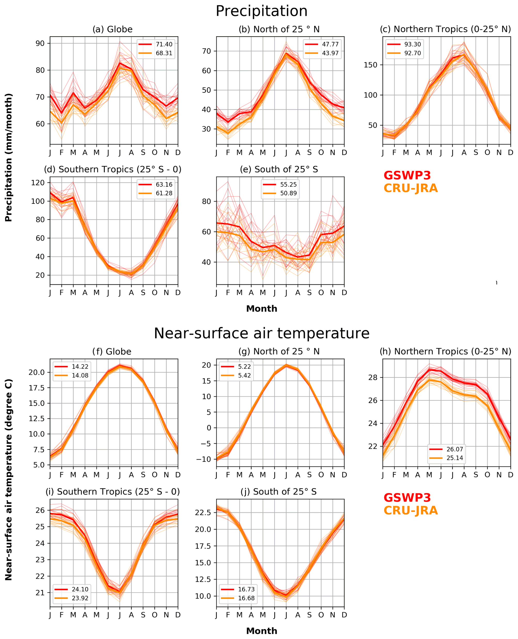
Figure A1 Comparison of monthly precipitation (upper panel) and temperature (lower panel) for five global regions (global, north of 25^∘ N, northern and southern tropics, and south of 25^∘ S) from the CRU-JRA and GSWP3 meteorological forcing data sets that are used to drive the CLASSIC model. The global and regional averages exclude Greenland and Antarctica. The legend entries show the annual mean values averaged over the 1997–2016 period. The thin lines show individual years, and the thick line is their average.

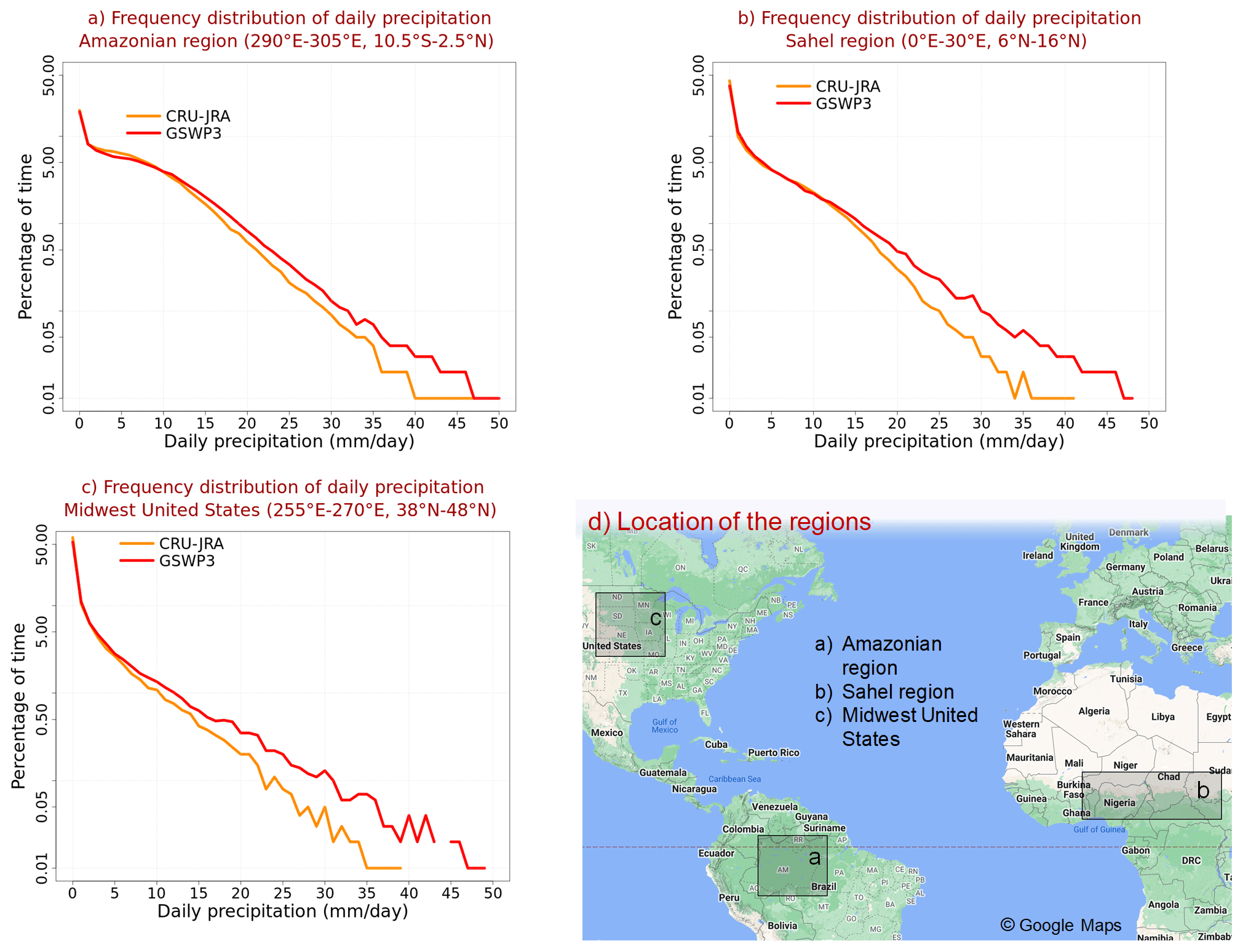
Figure A2 Comparison of the frequency distribution of daily precipitation between the CRU-JRA and GSWP3 meteorological data sets for three broad regions and the period 1997–2016: (a) the Amazonian region, (b) the Sahel region, and (c) the Midwest United States. The frequency is represented as a percentage of time; daily precipitation is between x and x+1 mm d⁻¹, where x is the value on the x axis; (d) shows the location of these broad regions. The underlying map in (d) is from Google Maps.

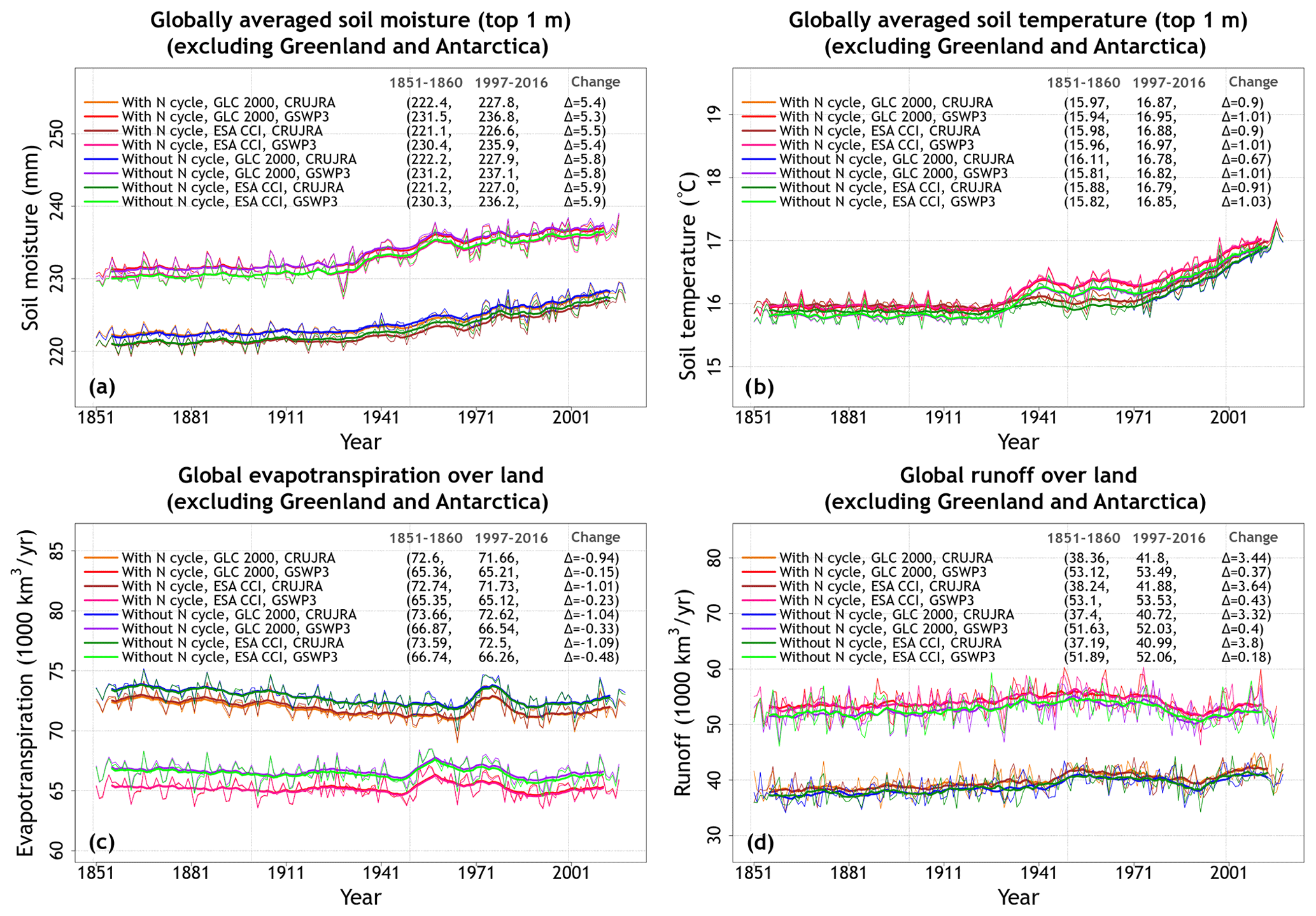
Figure A3 Time series of simulated globally averaged annual soil moisture (a) and soil temperature (b) in the top 1 m, global annual evapotranspiration (c), and runoff (d) from the eight simulations summarized in Table 1. The thin lines show the individual years, and the thick lines show their 11-year moving average. Model values averaged over the pre-industrial (1851–1860) and present-day (1997–2016) time periods, and their difference, are also shown.

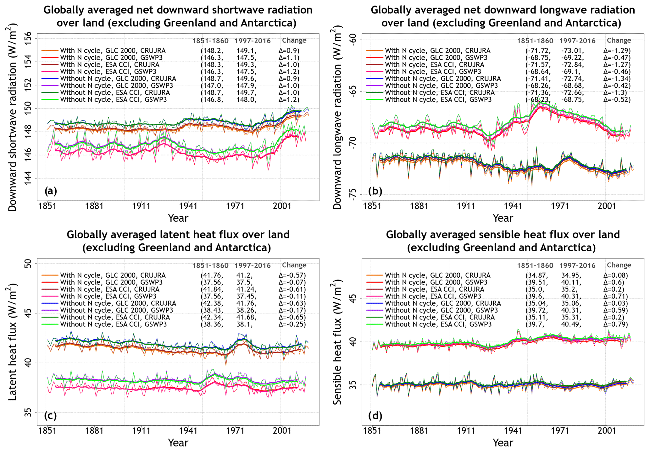
Figure A4 Time series of simulated globally averaged annual energy fluxes from the eight simulations summarized in Table 1; (a) shows net downward shortwave radiation, (b) shows net downward longwave radiation, (c) shows latent heat flux, and (d) shows sensible heat flux. The thin lines show the individual years, and the thick lines show their 11-year moving average. Model values averaged over the pre-industrial (1851–1860) and present-day (1997–2016) time periods, and their difference, are also shown for individual simulations.

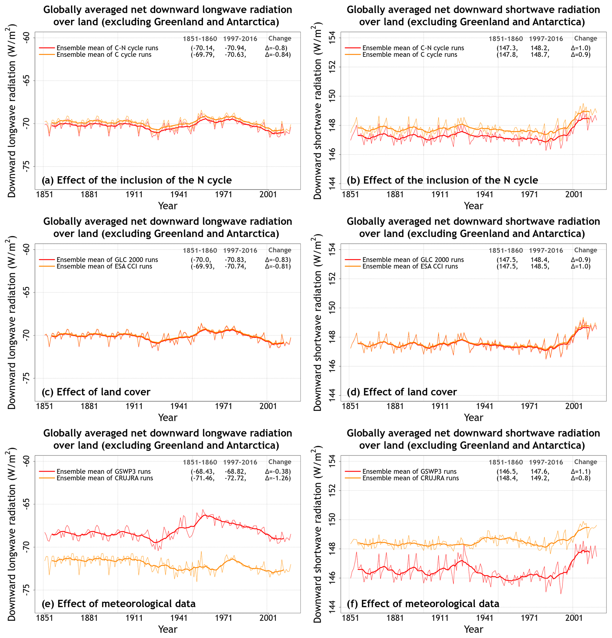
Figure A5 Time series of globally averaged annual net downward longwave and shortwave radiation (over all land area excluding Greenland and Antarctica), each averaged over the four ensemble members that are driven with and without N cycle (a, b), that are driven with GLC-2000- and ESA-CCI-based land cover (c, d), and that are driven with GSWP3 and CRU-JRA meteorological data (e, f). The thin lines show the individual years, and the thick lines show their 11-year moving average. Model values averaged over the pre-industrial (1851–1860) and present-day (1997–2016) time periods, and their difference, are also shown.

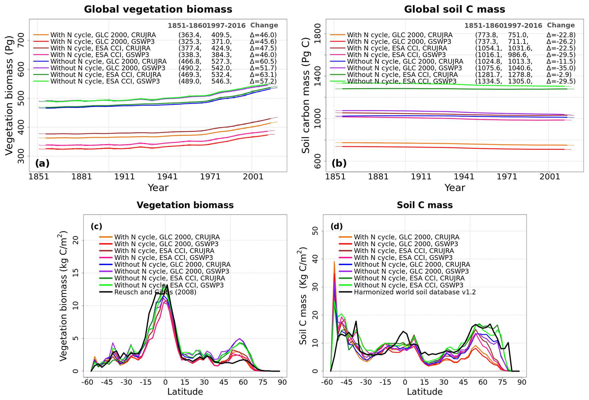
Figure A6 Time series of simulated global annual vegetation carbon mass (a) and soil carbon (b) from the eight simulations summarized in Table 1. The global totals exclude Greenland and Antarctica; (c) and (d) show the zonally averaged values of vegetation carbon mass and soil carbon mass over land from the eight simulations averaged over the 1997-2016 period. The thin lines show the individual years, and the thick lines show their 11-year moving average in (a) and (b). Model values averaged over the pre-industrial (1851–1860) and present-day (1997–2016) time periods, and their difference, are also shown in (a) and (b).

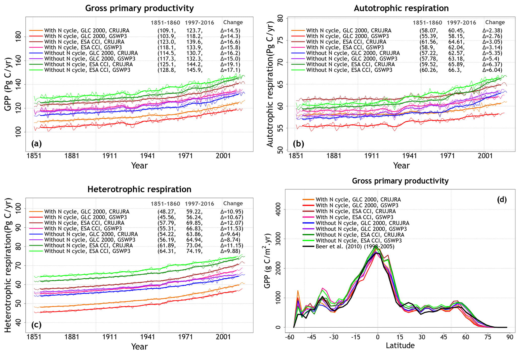
Figure A7 Time series of simulated global annual gross primary productivity (GPP) (a), autotrophic respiration (b), and heterotrophic respiration (c) from the eight simulations summarized in Table 1; (d) shows the zonally averaged values of GPP from the eight simulations averaged over the 1997–2016 period for each simulation. The thin lines show the individual years, and the thick lines show their 11-year moving average in (a) to (c). Model values averaged over the pre-industrial (1851–1860) and present-day (1997–2016) time periods, and their difference, are also shown in (a) to (c).

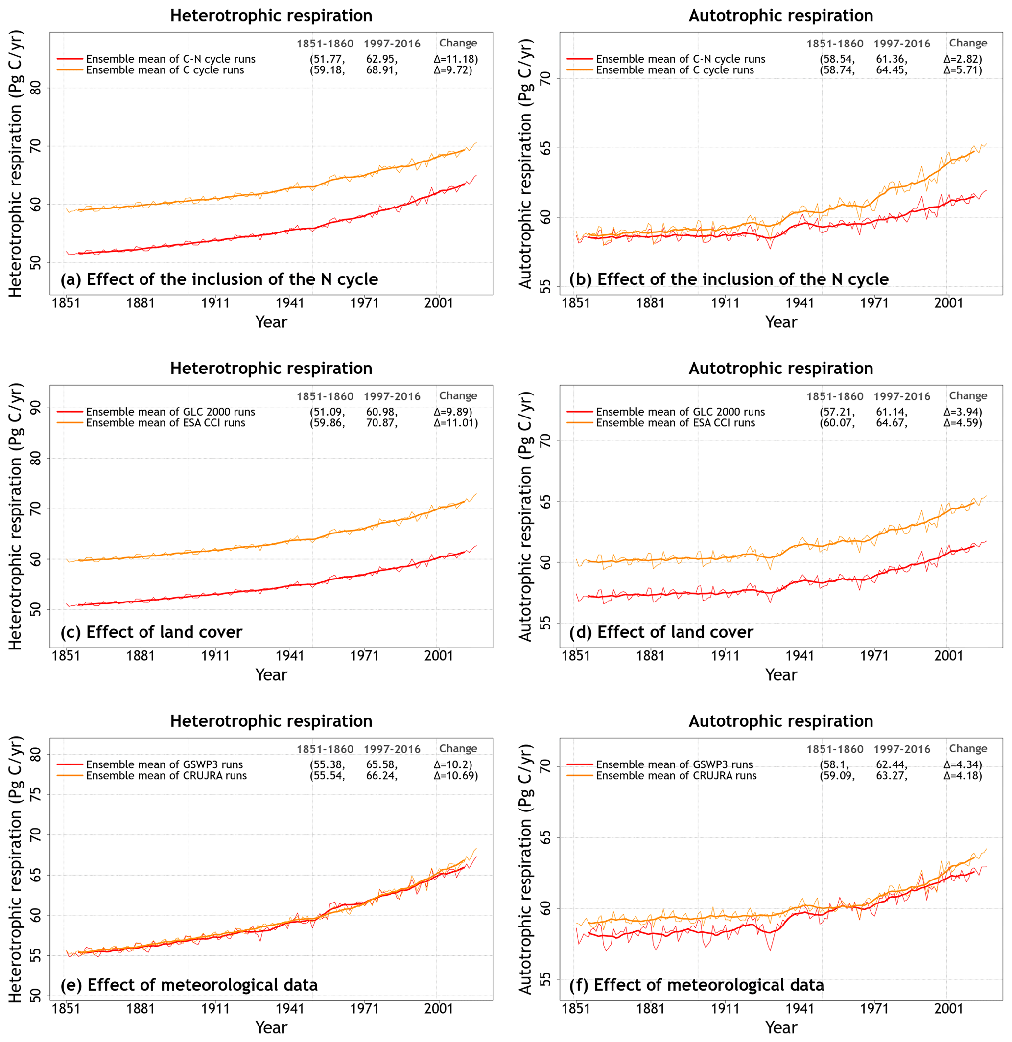
Figure A8 Time series of global heterotrophic and autotrophic respiration (over all land area excluding Greenland and Antarctica), each averaged over the four ensemble members that are driven with and without an interactive N cycle (a, b), that are driven with the GLC-2000- and ESA-CCI-based land cover (c, d), and that are driven with the GSWP3 and CRU-JRA meteorological data (e, f). The thin lines show the individual years, and the thick lines show their 11-year moving average. Model values averaged over the pre-industrial (1851–1860) and present-day (1997–2016) time periods, and their difference, are also shown.

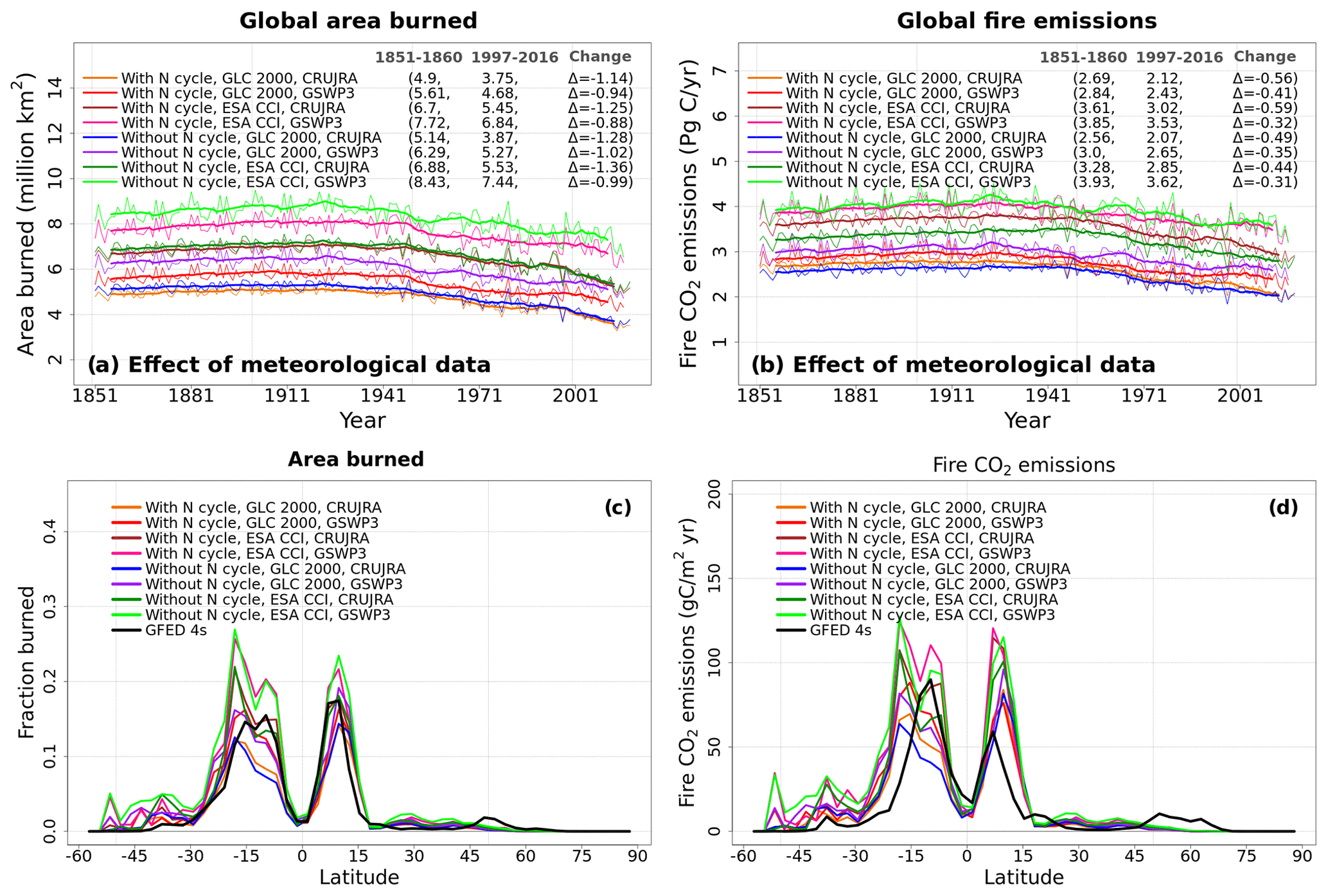
Figure A9 Time series of simulated global annual area burned (a) and fire CO₂ emissions (b) from the eight simulations summarized in Table 1; (c) and (d) show the zonally averaged area burned and fire CO₂ emissions from the eight simulations averaged over the 1997–2016 period. The thin lines for the time series show the individual years, and the thick lines show their 11-year moving average. Model values averaged over the pre-industrial (1851–1860) and present-day (1997–2016) time periods, and their difference, are also shown for (a) and (b).

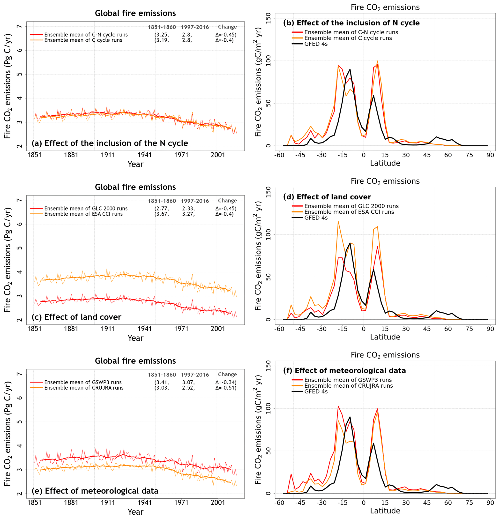
Figure A10 Time series of global fire CO₂ emissions (over all land area excluding Greenland and Antarctica) (a, c, e) and their zonally averaged values (b, d, f) averaged over the four ensemble members that are driven with and without an interactive N cycle (a, b), that are driven with the GLC-2000- and ESA-CCI-based land cover (c, d), and that are driven with GSWP3 and CRU-JRA meteorological data (e, f). The thin lines for the time series show the individual years, and the thick lines show their 11-year moving average in (a), (c), and (e). Model values averaged over the pre-industrial (1851–1860) and present-day (1997–2016) time periods, and their difference, are also shown for (a), (c), and (e).

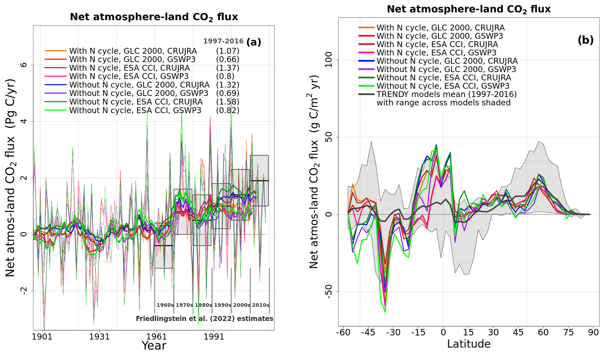
Figure A11 Time series of simulated global annual net atmosphere–land CO₂ flux (a) and its zonally averaged values from the eight simulations summarized in Table 1 averaged over the 1997–2016 period. In (a) simulated annual net atmosphere–land CO₂ flux values are compared to the estimates from the Global Carbon Project (Friedlingstein et al., 2022). The thin lines for the time series in (a) show the individual years, and the thick lines show their 11-year moving average. In (b) the simulated zonally averaged values are compared to the range from 11 models that contributed to the TRENDY 2020 intercomparison and are averaged over the 1997–2016 period.

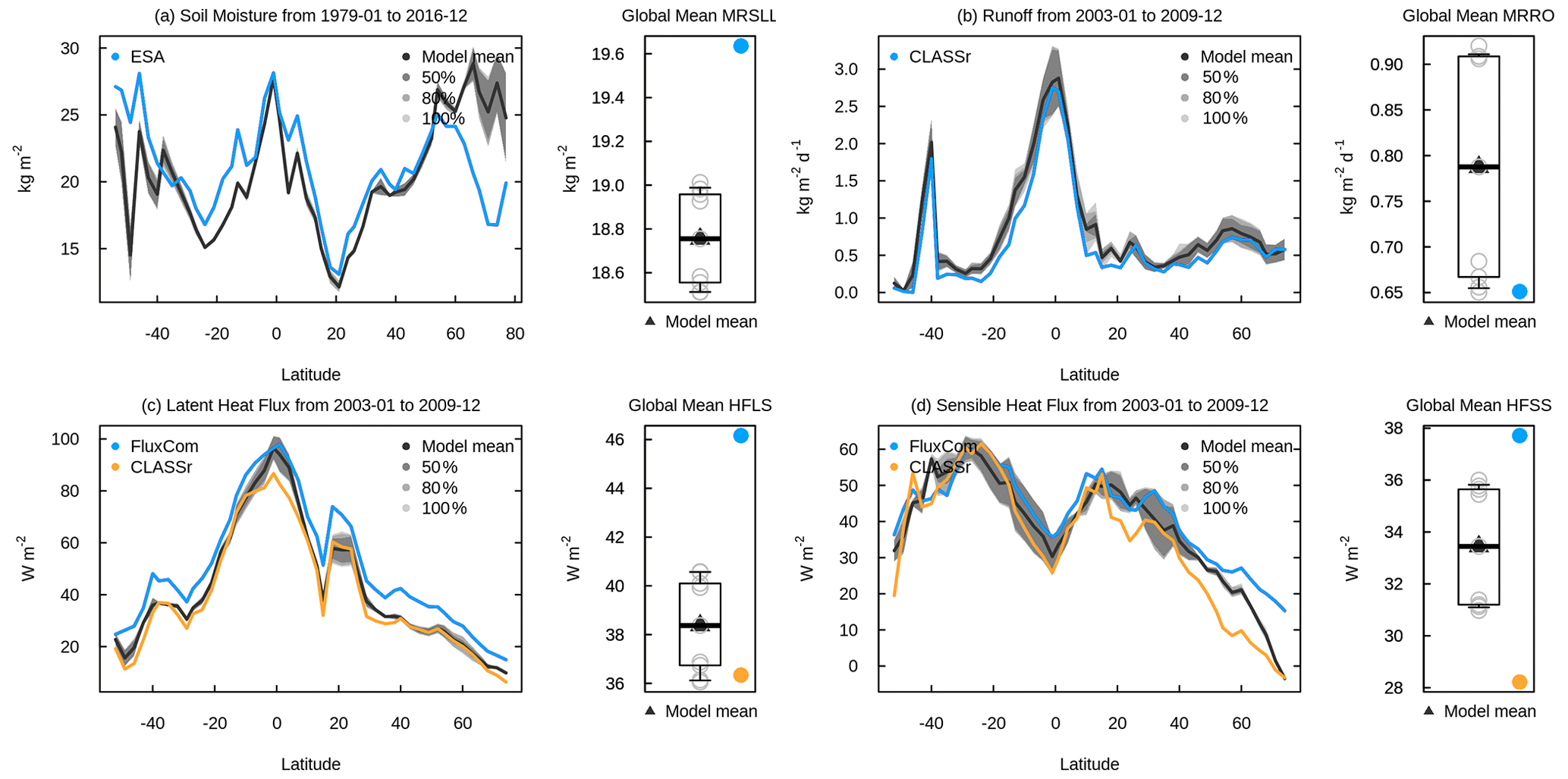
Figure A12 Zonally averaged values of soil moisture (a), runoff (b), latent heat flux (c), and sensible heat flux (d) from the eight simulations summarized in Table 1. The model results are shown as their mean (black) and the spread across the eight simulations indicated by 50 %, 80 %, and 100 % ranges in different shades of grey. The observation-based estimates used in AMBER to calculate scores are shown in coloured lines.

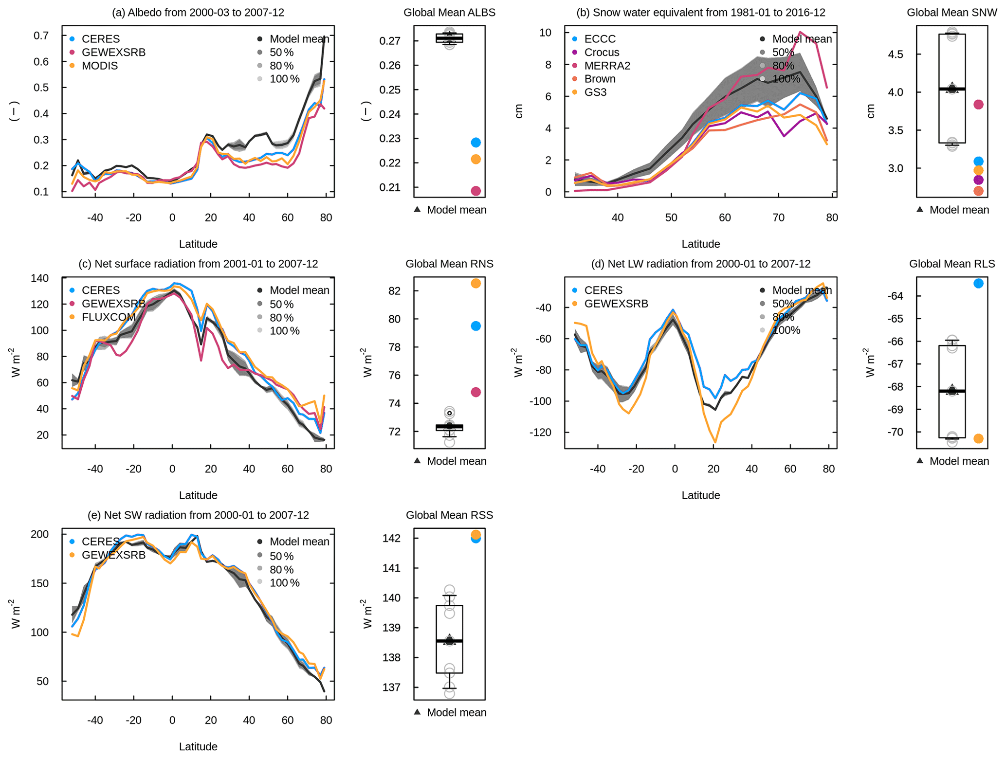
Figure A13 Zonally averaged values of surface albedo (a), snow water equivalent (b), net surface radiation (c), net longwave radiation (d), and net shortwave radiation (e) from the eight simulations summarized in Table 1. The model results are shown as their mean (black) and the spread across the eight simulations indicated by 50 %, 80 %, and 100 % ranges in different shades of grey. The observation-based estimates used in AMBER to calculate scores are shown in coloured lines.