Mapping soil organic carbon fractions for Australia, their stocks, and uncertainty

Soil organic carbon (SOC) is the largest terrestrial carbon pool. SOC is composed of a continuous set of compounds with different chemical compositions, origins, and susceptibilities to decomposition that are commonly separated into pools characterised by different responses to anthropogenic and environmental disturbance. Here we map the contribution of three SOC fractions to the total SOC content of Australia's soils. The three SOC fractions, mineral-associated organic carbon (MAOC), particulate organic carbon (POC), and pyrogenic organic carbon (PyOC), represent SOC composition with distinct turnover rates, chemistry, and pathway formation. Data for MAOC, POC, and PyOC were obtained with near- and mid-infrared spectral models calibrated with measured SOC fractions. We transformed the data using an isometric-log-ratio (ilr) transformation to account for the closed compositional nature of SOC fractions. The resulting back-transformed ilr components were mapped across Australia. SOC fraction stocks for 0–30 cm were derived with maps of total organic carbon concentration, bulk density, coarse fragments, and soil thickness. Mapping was done by a quantile regression forest fitted with the ilr-transformed data and a large set of environmental variables as predictors. The resulting maps along with the quantified uncertainty show the unique spatial pattern of SOC fractions in Australia. MAOC dominated the total SOC with an average of 59 % ± 17 %, whereas 28 % ± 17 % was PyOC and 13 % ± 11 % was POC. The allocation of total organic carbon (TOC) to the MAOC fractions increased with depth. SOC vulnerability (i.e. $\text{POC}/[\text{MAOC}+\text{PyOC}]$) was greater in areas with Mediterranean and temperate climates. TOC and the distribution among fractions were the most influential variables in SOC fraction uncertainty. Further, the diversity of climatic and pedological conditions suggests that different mechanisms will control SOC stabilisation and dynamics across the continent, as shown by the model covariates' importance metric. We estimated the total SOC stocks (0–30 cm) to be 13 Pg MAOC, 2 Pg POC, and 5 Pg PyOC, which is consistent with previous estimates. The maps of SOC fractions and their stocks can be used for modelling SOC dynamics and forecasting changes in SOC stocks as a response to land use change, management, and climate change.

1 Introduction

Soils are the main organic carbon pool in terrestrial ecosystems, storing around two-thirds of the total C. The global soil organic carbon (SOC) stock is estimated to be around 1500 Pg C for the first metre of soil (Jobbagy and Jackson, 2000), with other estimates ranging from 504 to 3000 Pg C (Scharlemann et al., 2014). Changes in SOC storage and dynamics can alter the ecosystem C balance and determine whether soils become C sources or sinks from local to global scales (Friedlingstein et al., 2020). SOC is strongly linked to most soil properties and functions (e.g. nutrient and water storage and cycling, habitat provisioning, and biodiversity) (van Leeuwen et al., 2019) and hence is used as a general indicator of soil quality/capacity (Schoenholtz et al., 2000; Bunemann et al., 2018) and soil health/condition.

Soil organic matter consists of a continuum of compounds with different chemical compositions, origins (above-ground litter, dead roots, rhizodeposition, microbial-derived), degrees of microbial processing and decomposition, and turnover times (Lehmann and Kleber, 2015). SOC is the main component of soil organic matter and varies in spatial and temporal dynamics. SOC is protected against microbial decomposition by several stabilisation mechanisms which have been generally grouped into (1) selective preservation due to biochemical recalcitrance, (2) chemical stabilisation via interactions between organic compounds and mineral surfaces or metal cations, and (3) physical protection by the inaccessibility of decomposers to the organic matter (Sollins et al., 1996; von Lützow et al., 2006; Rowley et al., 2018). Spatial inaccessibility and interactions between the mineral surfaces of silt- and clay-sized particles and organic compounds are considered the major mechanisms for mid- and long-term SOC stability (von Lützow et al., 2006), whereas an increasing body of literature questions the relevance of biochemical recalcitrance for long-term persistence of SOC (Schmidt et al., 2011). However, the hierarchy between stabilisation mechanisms varies with the pedoclimatic context, land use, and SOC fraction.

A myriad of physical, chemical, or combined fractionation methods have been designed for separating SOC into operational pools characterised by specific stabilisation mechanisms, chemical compositions, and distinct turnover rates, and yet it is difficult to isolate fractions that correspond to functional SOC pools (von Lützow et al., 2007). Some fractionation schemes were adapted to quantify conceptual SOC pools from established C dynamics models, e.g. the Rothamsted C model (RothC, Jenkinson and Rayner, 1977) from measured SOC fractions (Poeplau et al., 2013; Zimmermann et al., 2007). However, there can be some discrepancies between the predicted SOC pools when the model is initialised with modelled SOC pools from equilibrium runs or from measured SOC fractions (Poeplau et al., 2013). Other biogeochemical models have been conceptualised and calibrated with functional and measurable SOC fractions to overcome these differences (Robertson et al., 2019) but often require the determination of many SOC fractions. A comparison of several fractionation schemes (Poeplau et al., 2018) suggests that size separation into silt + clay (<53 µm) (i.e. mineral-associated organic carbon – MAOC) and sand-sized particles (>53 µm) (i.e. particulate organic carbon – POC) may suffice to differentiate pools with distinct turnover rates, chemistry, and pathway formation (Lavallee et al., 2020). MAOC is predominantly composed of low-molecular-weight molecules of microbial origin (e.g. microbial metabolites, necromass) (Miltner et al., 2012; Kallenbach et al., 2016; Liang et al., 2019), leachates from plant litter, and rhizodeposition (Villarino et al., 2021), which are protected through sorption to mineral surfaces or occluded inside microaggregates (Lavallee et al., 2020). POC is mainly composed of partially decomposed plant litter and roots and fungal-derived compounds (Baisden et al., 2002; Gregorich et al., 2006; Geng et al., 2019; Villarino et al., 2021) that can be found free or inside macroaggregates (Rabbi et al., 2014). MAOC has a lower C:N ratio, a higher proportion of microbial-derived and proteinaceous compounds (Kleber et al., 2007; Knicker, 2011), and a longer mean residence time (decades to centuries) than POC (mean residence time of years to decades) (Baisden et al., 2002; Gregorich et al., 2006; von Lützow et al., 2007; Heckman et al., 2022). Separating SOC into POC and MAOC has been proposed as a simple and effective way to conceptualise and model SOC dynamics (Lavallee et al., 2020) and has been applied to predict the vulnerability of SOC to future climate scenarios (Lugato et al., 2022).

In Australia, the long history of burning suggests that pyrogenic organic carbon (PyOC) is an additional important component of SOC (Lehmann et al., 2008). PyOC refers to charred residues derived from incomplete combustion of organic matter (also known as charcoal or black carbon) (Lutfalla et al., 2017). PyOC is composed of a continuum of organic compounds thermally altered by fire, and its chemical composition and pool size depend on the technique used for its determination (Zimmerman and Mitra, 2017). PyOC is considered a relatively stable SOC fraction with a turnover time that ranges from decades to centuries (Singh et al., 2012), protected from decomposition by the biochemical recalcitrance of condensed aromatic C (Lavallee et al., 2019). However, turnover rates previously assessed from centuries to many millennia may have overestimated its persistence in soil (Singh et al., 2012; Lutfalla et al., 2017). PyOC can be found in both POC and MAOC fractions (Lavallee et al., 2019). Beyond the biochemical recalcitrance, which would be the main stabilisation mechanism of PyOC in the POC fraction (e.g. free PyOC not associated with clay- and silt-sized mineral particles), PyOC can also interact with mineral phases and be protected inside microaggregates or through adsorption (Burgeon et al., 2021). Zimmerman and Mitra (2017) suggest that PyOC (e.g. naturally occurring or added as biochar) may promote the stabilisation of non-PyOC by enhancing the creation of microaggregates and sorption onto existing organo–mineral complexes. PyOC represents on average 14 %–26 % of total SOC and can reach up to 60 %–80 % of SOC (Lehmann et al., 2008; Reisser et al., 2016). Globally, PyOC stocks are not controlled by fire intensity and return interval but are explained by soil properties and climate (Reisser et al., 2016). However, in systems with local records of fire history, PyOC content increased in sites with high-frequency fires (Reisser et al., 2016). In Australia, fire is an important driver of ecological processes, and bush-fire frequency has increased in recent decades (Dutta et al., 2016). Hence, PyOC can represent a large proportion of total SOC in some Australian regions (Lehmann et al., 2008).

Mapping and quantifying the stocks of SOC fractions can be used for modelling SOC dynamics and forecasting changes in SOC stocks as a response to land use change, management, and climate change (Lugato et al., 2022; Xu et al., 2011; Wiesmeier et al., 2016). High-resolution maps of SOC fractions can inform agricultural management at the farm scale and be incorporated into the design of climate change and soil security policies at the state and national levels (Dangal et al., 2022). The objective of this study was to map the contribution of SOC fractions (MAOC, POC, and PyOC) to the total SOC in the top 30 cm of the soil and update the Soil and Landscape Grid of Australia (SLGA) (Grundy et al., 2015) products for SOC fraction stocks (Viscarra Rossel et al., 2019). These digital soil maps will be part of the v2 SLGA for Australia, following the principles of transparency, reproducibility, and updatability as new data become available (Malone and Searle, 2021).

2 Materials and methods

The methodology implemented in this study consists of two main steps: (1) prediction of SOC fractions across the soil spectral libraries available for Australia with different spectral models calibrated with measured SOC fraction data from the Australian Soil Carbon Research Program (SCaRP) (Baldock et al., 2013b) and (2) mapping of the proportions of SOC fractions after applying the isometric-log-ratio (ilr) transformation to account for the compositional nature of the data (i.e. the proportion of SOC fractions sums to 100 %). Previous studies modelled SOC fraction stocks or concentrations (Sanderman et al., 2021; Viscarra Rossel et al., 2019), but we found some difficulties in implementing such an approach (see Sect. 2.5) and hence mapped proportions of SOC. Finally, we calculated SOC fraction stocks for the 0–30 cm topsoil using data from SLGA maps of total organic carbon (TOC) concentration (Wadoux et al., 2022), bulk density (Viscarra Rossel et al., 2015), coarse fragments (this study), and soil thickness (Malone and Searle, 2020).

2.1 Study area

The study area covers the continent of Australia, including Tasmania and near-shore small islands. In Australia there are six major climatic regions following the Köppen classification. In the north, there are hot, humid summers in equatorial, tropical, and sub-tropical regions. Summers are hot and dry, with mild to cold winters in grasslands and desert regions in the interior. Temperate areas in the southern coastal band have cold winters and warm summers that are mild at higher elevations and latitudes. Vast areas of the continent are very dry, with precipitation increasing towards the coast and elevation in the mountains of the eastern uplands. Australia is characterised by flat and low-relief vast areas where the tectonic stability and lack of glaciation have preserved a deeply weathered mantle that dates from the Tertiary (McKenzie et al., 2004). The distribution of soils in many regions depends on the stripping of this weathered mantle, while in other areas the dominant drivers of landforms and soils are water, fluvial, and aeolian erosion and depositional processes (McKenzie et al., 2004). Younger soils are found mainly in the east, along the Great Divide (McKenzie et al., 2004). The dominant soil orders according to the Australian Soil Classification (Isbell et al., 1997) are Kandosol (30 % of the area), Tenosol (20 %), Vertosol (14 %), Rudosol (8 %), Calcarosol (8 %), and Chromosol (7 %) (Searle, 2021). In 2015–2016 most of the area was dedicated to primary production, with 48 % of the continent used for livestock grazing (42 % native vegetation and 6 % modified pastures) and less than 5 % dedicated to dryland and irrigated cropping. About 9.5 % of Australia is allocated to nature conservation and 18 % is protected managed resources (Australian Bureau of Agricultural and Resource Economics and Sciences, 2022).

2.2 SCaRP dataset – sampling design and SOC fractionation scheme

The soil-sampling design and SOC fractionation protocol of SCaRP are described in detail in Sanderman et al. (2011) and Baldock et al. (2013b). The objective of SCaRP was to characterise SOC stocks and the composition of agricultural topsoils (0–30 cm) and their response to agricultural practices. Plots of 25 m² were laid in 4526 sites representative of the different combinations of agricultural management and soil types across Australia between 2008 and 2012. At each plot, soil samples were collected randomly at 10 nodes of a 5 m×5 m grid with a soil corer (≥4 cm diameter) by depth interval (0–10, 10–20, 20–30 cm) and composited by layer. In addition, at least three measurements of bulk density by depth interval were taken at each plot, although the methods varied between states to accommodate the soil type. A sub-set of 312 samples representative of the range of TOC content (1.2–90.9 mg C g⁻¹ soil) found among the whole dataset (N=24 495 samples) and different soil types and biomes was subject to fractionation following the protocol described in detail in Baldock et al. (2013c). The size and chemical fractionation scheme divided SOC into MAOC, POC, and PyOC. MAOC and PyOC were originally defined as humic organic carbon and resistant organic carbon (ROC) in Baldock et al. (2013c), and although the ROC fraction may not correspond completely to PyOC, we changed the terminology to match the recent literature. A 10 g aliquot of air-dried soil ≤2 mm was dispersed with 5 g L⁻¹ sodium hexametaphosphate and separated into coarse (>50 µm) and fine (<50 µm) fractions with wet sieving using an automated sieve-shaker system (Baldock et al., 2013c). The TOC concentrations of the coarse and fine fractions were analysed with high-temperature oxidative combustion after the removal of inorganic carbon with 5 %–6 % H₂SO₃ if carbonates were present (method 6B3a, Rayment and Lyons, 2011). Solid-state ¹³C nuclear-magnetic-resonance (¹³C NMR) spectroscopy analyses were conducted on both the coarse (>50 µm) and fine (<50 µm) fractions. ¹³C NMR is a semi-quantitative method that is commonly used to measure the proportion of aromatic C compounds in soil and organic matter samples. The proportion of poly-aryl C and aryl C that could be defined as lignin was determined and used as an estimate of PyOC. We note that, whereas the chemical signature of the poly-aryl C is consistent with and likely dominated by charcoal and charred plant residues, it may also indicate the presence of compounds of non-pyrogenic origin (Baldock et al., 2013c). POC and MAOC contents (mg C-fraction g⁻¹ soil) were calculated by subtracting the proportion of PyOC in each fraction with the following equations (Baldock et al., 2013c):

$$\begin{array}{}\text{(1)}& {\displaystyle }\text{POC}=(\mathrm{2000}-\mathrm{50}\mathrm{\mu }\mathrm{m}\mathrm{OC})(\mathrm{1}-{\text{fPyOC}}_{\mathrm{2000}}){\text{MF}}_{\mathrm{2000}},\text{(2)}& {\displaystyle }\text{MAOC}=(\le \mathrm{50}\mathrm{\mu }\mathrm{m}\mathrm{OC})(\mathrm{1}-{\text{fPyOC}}_{\mathrm{50}}){\text{MF}}_{\mathrm{50}},\text{(3)}& {\displaystyle }\begin{array}{rl}\text{PyOC}=& (\mathrm{2000}-\mathrm{50}\mathrm{\mu }\mathrm{m}\mathrm{OC})\left({\text{fPyOC}}_{\mathrm{2000}}\right){\text{MF}}_{\mathrm{2000}}\\ & +(\le \mathrm{50}\mathrm{\mu }\mathrm{m}\mathrm{OC})\left({\text{fPyOC}}_{\mathrm{50}}\right){\text{MF}}_{\mathrm{50}},\end{array}\end{array}$$

where 2000–50 µm OC is the measured TOC content in the coarse fraction (mg C g⁻¹ 2000–50 µm fraction), fPyOC₂₀₀₀ is the proportion of TOC attributed to poly-aryl C in the coarse fraction, MF₂₀₀₀ is the proportion of soil mass found in the coarse fraction (g 2000–50 µm fraction$/$g ≤2 mm soil), ≤50 µm OC is the measured TOC content in the fine fraction ($\mathrm{mg}\mathrm{C}{\mathrm{g}}^{-\mathrm{1}}\le \mathrm{50}\mathrm{\mu }\mathrm{m}\mathrm{fraction}$), fPyOC₅₀ is the proportion of TOC attributed to poly-aryl C in the fine fraction, and MF₅₀ is the proportion of soil mass found in the fine fraction (g≤50 µm fraction$/$g≤2 mm soil).

2.3 Spectral datasets and harmonisation

Four spectral soil datasets were combined in this study: SCaRP (4526 sites and 24 495 soil specimens; Baldock et al., 2013a), the Australian Soil Archive mid-infrared (MIR) spectral library (703 sites and 4300 soil specimens; AusSpecMIR) (Hicks et al., 2015), an additional MIR library of specimens from the Australian Soil Archive that was not included in the Hicks et al. (2015) work (346 sites and 429 soil specimens; AusSpecMIR2), and the Australian Soil Archive visible and near-infrared (Vis–NIR) spectral library (4533 sites and 25 174 soil specimens; AusSpecNIR). The majority but not all of these Vis–NIR data were described in Viscarra Rossel and Hicks (2015).

The AusSpecNIR library also contained a sub-set (309) of the soil specimens described in Viscarra Rossel and Hicks (2015), which contain measures of soil carbon fractions from selected SCaRP soil specimens and associated Vis–NIR spectra. The spectra were collected using the same instrument that was used to derive the Australian Soil Archive Vis–NIR spectral library. The AusSpecNIR library contained further data from the Terrestrial Ecosystem Research Network (TERN) Ecosystem Surveillance plots (Sparrow et al., 2020; Malone et al., 2020), increasing the representation of non-agricultural soils (rangelands, forests, woodlands) of the combined datasets (Fig. 1b). With these TERN data, vegetation and soils are sampled in more than 800 permanent plots laid with stratified random sampling across bioregions (i.e. zones with similar landforms, vegetation, and climate, analogous to ecoregions) (Sparrow et al., 2020). Soil samples are taken from three depth intervals (0–10, 10–20, 20–30 cm) in nine locations within a 100 m×100 m plot (Sparrow et al., 2020), for a total of 15 157 soil specimens (with associated Vis–NIR spectra) at 5711 georeferenced sampling points.

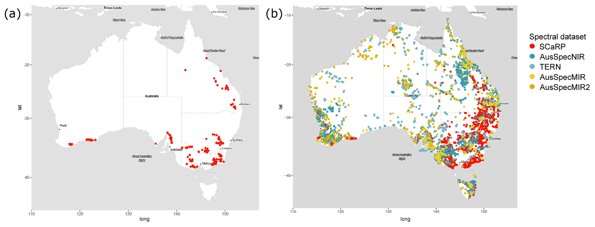
Figure 1 (a) Location of SCaRP soil samples subject to fractionation (n=312) by Baldock et al. (2013c). (b) Soil spectral datasets combined for mapping soil organic carbon fractions. TERN samples are part of the AusSpecNIR library.

Excepting those with soil carbon fraction measurements, multiple soil samples (approximately 700) were represented in both AusSpecMIR and AusSpecNIR, and duplicates were removed from AusSpecNIR for the subsequent modelling processes.

The ScaRP spectral library was produced with a Nicolet 6700 FTIR spectrometer (Thermo Fisher Scientific Inc., Waltham, MA, USA) equipped with a KBr beam splitter, a DTGS detector, and an AutoDiff automated diffuse-reflectance accessory (Pike Technologies, Madison, WI, USA). Spectra were acquired over the range 8000–400 cm⁻¹ with a resolution of 8 cm⁻¹. The spectrum of each soil sample was the average of 60 scans. The AusSpecMIR spectral library was created with a Bruker FT-IR Vertex70 spectrometer. This instrument is fitted with a mercury cadmium telluride detector that is liquid-nitrogen-cooled to improve the signal-to-noise ratio and has a spectral range of 7500–600 cm⁻¹ at 4 cm⁻¹ resolution. AusSpecMIR2 was measured with a Bruker FT-IR Invenio spectrometer with a similar liquid-nitrogen cooling system and a spectral range of 7500–600 cm⁻¹ at 4 cm⁻¹ resolution. Soil samples from AusSpecMIR and AusSpecMIR2 were scanned in quadruplicate. Diffuse-reflectance spectra for the AusSpecNIR library were collected with a Labspec^® Vis–NIR spectrometer (PANalytical Inc., Boulder, CO, USA) for the range 350–2500 nm at 1 nm resolution. Each spectrum was the average of 30 scans, and up to four spectra were collected for each soil sample.

SCaRP spectra were baseline-corrected and mean-centred prior to subsequent analyses but were not subject to additional pre-processing. Pre-processing of the AusSpecNIR spectra consisted of spectral trimming (453–2500 nm), a Savitsky–Golay smoothing filter, conversion of reflectance to absorbance, and standard normal variate transformation. AusSpecMIR and AusSpecMIR2 were both pre-processed with the following steps: (1) spectral resolution and range harmonisation. All spectra were resampled using a smoothing spline function to a common 2 cm⁻¹ resolution. The spectral range was set to 6500 to 598 cm⁻¹, (2) the Savitsky–Golay smoothing filter with a 22 cm⁻¹ local neighbourhood, (3) conversion from reflectance to absorbance units, and (4) standard normal variate transformation.

2.4 Spectral models and predictions of SOC fractions

SOC fractions' contents (mg C g⁻¹ soil) of SCaRP were previously estimated with partial-least-squares-regression (PLSR) models by Baldock et al. (2013a). Baldock et al. (2013a) reported cross-validation results (squared-root-transformed SOC fractions' contents) with R² values of 0.84, 0.88, and 0.85 and root-mean-squared errors (RMSEs) of 0.43, 0.40, and 0.32 for POC, MAOC, and PyOC, respectively.

SOC fractions' contents for AusSpecMIR and AusSpecMIR2 were estimated with a new set of spectral predictive functions (Malone and Wadoux, 2021). Spectral harmonisations using piecewise direct standardisation (Bouveresse and Massart, 1996; Ge et al., 2011) was used to align spectra collected for SCaRP and AusSpecMIR2 to the AusSpecMIR spectrometer. Approximately 200 soil samples from the SCaRP dataset were measured with the Bruker FT-IR Vertex70 spectrometer, following the estimate of parameters to harmonise the SCaRP library with AusSpecMIR. Similarly, the AusSpecMIR2 was harmonised with AusSpecMIR with piecewise direct standardisation (PDS) using a standard of 300 soil samples measured with both instruments.

Soil spectral model functions were developed with the 312 SCaRP samples with data on SOC fraction concentration (mg C-SOC fraction g⁻¹ soil), TOC concentration (mg C g⁻¹ soil), and used PDS-harmonised spectra. The contents of SOC fractions were converted into percentages of TOC (summing up to 100 %) and modelled as compositional data. Hence, the ilr transformation was applied to the proportions of SOC fractions. The ilr generates a D−1-dimensional Euclidean vector, where D is the number of variables in the original variables (Aitchison, 1986). PLSR models with bootstrapping were used to predict the ilr-transformed SOC fractions. Out-of-bag validation statistics were calculated from the average of 50 model realisations on the back-transformed data. The average RMSEs for POC, MAOC, and PyOC were 6.2 %, 7.7 %, and 6.4 %, respectively. Lin's concordance correlation coefficient (ρ_c) values were 0.86, 0.76, and 0.70, and R² was 0.74, 0.61, and 0.52. When the percentages were back-transformed into SOC fractions' contents (mg C-SOC fraction g⁻¹ soil), the RMSEs were 2.1, 2.7, and 1.8 mg C g⁻¹ soil, ρ_c was 0.92, 0.95, and 0.90, and R² was 0.85, 0.88, and 0.77 for POC, MAOC, and PyOC, respectively.

SOC fractions' contents for the AusSpecNIR dataset were predicted with PLSR models calibrated with data on TOC concentration and SOC fractions' contents from the 309 SCaRP samples. Before modelling, the spectra were trimmed to the 453–2500 nm range, processed with a Savitsky–Golay smoothing filter, and transformed from reflectance to absorbance. We also applied the standard normal variate transformation, and then wavelet coefficients were derived. Similarly, as for the MIR datasets, spectral predictive functions were developed for ilr-transformed SOC fraction compositional data, and validation statistics were calculated for the back-transformed data. The validation statistics for the POC, MAOC, and PyOC models were, respectively, RMSEs of 5.0 %, 6.4 %, and 5.8 %, ρ_c of 0.92, 0.84, and 0.76, and R² of 0.83, 0.71, and 0.61 when validated as proportions of TOC. When the validation statistics were calculated for SOC fractions' contents, the RMSEs were 3.2, 4.0, and 2.3 mg C g⁻¹ soil, ρ_c 0.81, 0.87, and 0.80, and R² 0.65, 0.75, and 0.64 for POC, MAOC, and PyOC.

Fitted spectral models based on either MIR and Vis–NIR data were then extended to all data cases of the respective soil spectral libraries.

2.5 SOC fractions' data processing and depth standardisation

The georeferenced SOC fraction data from all libraries were projected to WGS84 (EPSG:4326) and collated. The data were filtered and processed to harmonise units, and duplicates and potentially wrong data entries (e.g. missing upper- or lower-horizon depths) were excluded. SOC predictions of the quadruplicated scans per soil sample were averaged as well as multiple soil samples per horizon by sampling location. SOC fraction concentrations (mg C-SOC fraction g⁻¹ soil) were transformed to the proportion of total SOC (% SOC). SOC potential vulnerability (Vp) was defined as the ratio of POC to the sum of MAOC and PyOC (Baldock et al., 2018), i.e. the proportion of the less-protected SOC fraction (POC) to the SOC fractions with stability by physico-chemical protection and recalcitrance and longer turnover rates. SOC fractions and Vp data were standardised to the first three depth intervals of the GlobalSoilMap (GSM) specifications (0–5, 5–15, 15–30 cm) (Arrouays et al., 2014) with equal-area quadratic splines (Bishop et al., 1999) (Fig. 2). For sampling locations with just one sampled horizon, this was converted to the GlobalSoilMap depth intervals (assigned to a single or several depth intervals) via aggregation with the slab function of the aqp R package (Beaudette et al., 2022). We calculated the mean and standard deviation of SOC fractions and Vp by the GlobalSoilMap depth interval and by biome (Olson et al., 2001). Extreme values of Vp were constrained to a maximum of 5 before calculating the summary statistics.

Figure 2 Locations of the spectral predictions standardised for the depths 0–5, 5–15, and 15–30 cm used as input data for digital soil mapping. Contribution of SOC fractions to total organic carbon (% TOC): MAOC, POC, PyOC, and Vp.

Modelling SOC fraction concentrations directly was the preferred option tested in preliminary work. We compared the sum of the predicted SOC fractions' contents with measured TOC. Pearson's r correlation coefficient was 0.56, but the sum of SOC fractions showed some extreme values (Fig. S1 in the Supplement). The mismatch between the sum of SOC fractions and measured TOC is most likely derived from the prediction error of the spectral models and to a minor extent from the TOC recoveries of the laboratory SOC fractionation data. We adjusted the SOC fractions' contents with measured TOC data extracted from the Soil Data Federator (Searle et al., 2021) and the Biome of Australian Soil Environments (BASE) contextual data (Bissett et al., 2016). However, the resulting dataset had a reduced spatial coverage and the maps exhibited unrealistic patterns. Hence, we preferred to use all available data and map the proportion of SOC fractions and SOC vulnerability.

The values of SOC proportions were modelled considering their compositional nature (i.e. multivariate data with positive values that sum up to a constant in the case of SOC fractions 100 %). The set of all compositional observations (S^D) is a simplex sample space, a sub-set of the real space ℝ^D. The ilr transformation (Egozcue et al., 2003) transposes S^D into multi-dimensional real space (ℝ^D−1), without the collinearity problems associated with other transformations, such as the centred log-ratio transformation (clr). Ilr is based on the choice of an orthonormal basis on the hyperplane in ℝ^D formed by the clr transformation. The ilr-transformation equation is defined:

$$\begin{array}{}\text{(4)}& \begin{array}{rl}{z}_i=\mathit{\text{ilr}}\left(x_i\right)=\sqrt{{\displaystyle \frac{i}{i+\mathrm{1}}}}\ln & \left({\displaystyle \frac{\sqrt[i]{{\prod }_{j=\mathrm{1}}^i{x}_j}}{x_{i+\mathrm{1}}}}\right),\\ & i=\mathrm{1},\mathrm{2},\mathrm{\dots },D-\mathrm{1}.\end{array}\end{array}$$

The inverse equation is defined as follows (Filzmoser and Hron, 2008):

$$\begin{array}{}\text{(5)}& {\displaystyle }{x}_i={\displaystyle \frac{\exp \left(y_i\right)}{{\sum }_{i=\mathrm{1}}^D\exp \left(y_i\right)}},i=\mathrm{1},\mathrm{2},\mathrm{\dots },D,\text{(6)}& {\displaystyle }\begin{array}{rl}{y}_i=\sum _{j=i}^D& {\displaystyle \frac{z_j}{\sqrt{j(j+\mathrm{1})}}}-\sqrt{{\displaystyle \frac{i-\mathrm{1}}{i}}}{z}_{i=\mathrm{1}}\\ & \text{with}{z}_{\mathrm{0}}=z_D=\mathrm{0}\text{for}i=\mathrm{1},\mathrm{2},\mathrm{\dots },D.\end{array}\end{array}$$

We applied the ilr transformation with the ilr function of the compositions R package (van den Boogaart et al., 2022), generating two variables hereafter referred to as ilr1 and ilr2. The predictions (ilr1 and ilr2) were back-transformed into MAOC, POC, and PyOC with the ilrInv function.

2.6 Coarse fragments

Data on the abundance of coarse fragments (particles>2 mm) and gravimetric content (wt %) were extracted using the TERN Soil Data Federator (https://esoil.io/TERNLandscapes/Public/Pages/SoilDataFederator/SoilDataFederator.html, last access: 22 June 2022) managed by CSIRO (Searle et al., 2021). The Soil Data Federator is a web API that compiles soil data from different institutions and government agencies throughout Australia. The abundance (% vol) is assessed visually in the field as part of the soil profile description using standards described in the Australian Soil and Land Survey Field Handbook (National Committee on Soil and Terrain, 2009). The abundance of rock fragments per soil horizon on the cut surface of the soil profile was grouped into six categories: very few (0 %–2 %), few (2 %–10 %), common (2 %–20 %), many (20 %–50 %), abundant (50 %–90 %), and very abundant (>90 %). The gravimetric content (% mass) is measured in the laboratory as percent mass of coarse fragments (particles>2 mm) from the whole soil. Here, we take the profile surface abundance of coarse fragments as a proxy for volumetric coarse fragments (CF_Vol). The data were cleaned and processed to exclude duplicates and wrong data entries (e.g. missing values). The observations of CF_Vol (%) were converted into GlobalSoilMap depth intervals with the slab function of the aqp R package (Beaudette et al., 2022), assigning the most probable class to each depth interval. The gravimetric coarse fragments were also standardised to the GlobalSoilMap depth intervals with equal-area quadratic splines (Bishop et al., 1999). Observations of gravimetric coarse-fragment content (CF_Mass) were transformed into volumetric ones with Eq. (4):

$$\begin{array}{}\text{(7)}& \begin{array}{rl}{\text{CF}}_{\text{Vol}}\left(\mathit{\%}\right)& ={\displaystyle \frac{{\text{Vol}}_{\text{CF}}}{{\text{Vol}}_{\text{WhSoil}}}}{\displaystyle \frac{\frac{{\text{Mass}}_{\text{CF}}}{{\mathit{\rho }}_{\text{CF}}}}{\frac{{\text{Mass}}_{\text{WhSoil}}}{{\mathit{\rho }}_{\text{WhSoil}}}}}\\ & ={\displaystyle \frac{{\text{CF}}_{\text{Mass}}\times {\mathit{\rho }}_{\text{WhSoil}}}{{\mathit{\rho }}_{\text{CF}}}},\end{array}\end{array}$$

where ρ_WhSoil is the bulk-density prediction for bulk soil from SLGA (Viscarra Rossel et al., 2015), ρ_CF is assumed to be 2.65 g cm⁻³ (Hurlbut and Klein, 1977, in McKenzie et al., 2002), and CF_Vol is the volumetric coarse-fragment content (continuous), which was assigned to the corresponding class. This resulted in CF_Vol observations for 110 308 locations (Fig. 3).

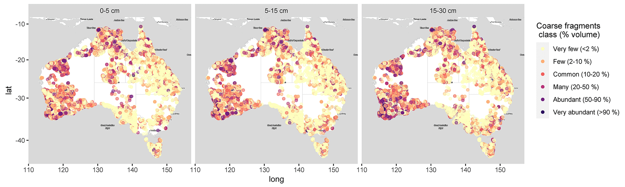
Figure 3 Calibration data on coarse-fragment (% vol) classes for the 0–5, 5–15, and 15–30 cm depth intervals.

2.7 Environmental covariates

We selected 61 spatially exhaustive covariates (90 m grid-cell size) for Australia made available by TERN, describing soil-forming factors and soil properties (Table 1), to calibrate scorpan models (McBratney et al., 2003). A scorpan model establishes quantitative relationships between soil properties or classes and other soil properties (s), climate (c), organisms (o), relief (r), parent material (p), age (a), and spatial position (n), i.e. $\text{soil}=f(s,c,o,r,p,a,n)$ (McBratney et al., 2003). We used the soil properties of clay and sand content for each GSM layer due to the relevant role of soil texture in SOC stabilisation. We selected 15 climatic covariates since climate is a relevant driver of SOC storage from the global to sub-regional scale (Wiesmeier et al., 2019), influencing both the SOC decomposition and the C input into the soil. The organism factor was represented by 22 covariates related to net primary productivity (e.g. normalised difference vegetation index, NDVI, enhanced vegetation index, EVI) and vegetation type, which influence the C allocation patterns, quantities, and pathways of C input (e.g. above-ground vs. below-ground). The long-term average NDVI calculated with Landsat 5 surface reflectance data was processed with Google Earth Engine. Eight relief covariates were surrogates for elevation, water flow, erosion processes, and sediment transport and accumulation, derived from the 3 s Shuttle Radar Topographic Mission (SRTM) (Farr et al., 2007). Gamma radiometrics, total magnetic intensity, and weathering intensity index (Wilford, 2012) were used as proxies for parent material and age. Gamma radiometrics inform on regolith's mineralogy and surface geochemistry. The concentrations and ratios of three radio elements (potassium, K, thorium, Th, uranium, U) are indicators of the lithology and degree of weathering (Wilford and Minty, 2007). The weathering intensity index map (Wilford, 2012) was generated from field-based data on the degree of bedrock weathering and multi-variate analysis using gamma radiometrics and relief covariates as predictors.

Table 1 List of environmental covariates with unit and associated reference when applicable. All covariates are in geographic coordinates with a 3 arcsec grid-cell (about 90 m×90 m) resolution with coordinate system WGS84 (EPSG:4326) and extent 10.0004–44.00042^∘ S, 112.99958–153.99958^∘ E.

The covariates were void-filled by a combination of plane fitting and inverse distance weighting (<0.5 % of pixels in the study area). The plane-fitting method was used to compute the average value of the neighbouring pixels, and otherwise an inverse-distance-weighting algorithm with default parameters was applied when the error in the plane fitting was large. This is the default implementation from ArcGIS software 10.5.

2.8 Modelling SOC fractions, SOC vulnerability, and coarse fragments

Quantile regression forests (Meinshausen, 2006) are a generalisation of the popular machine-learning algorithm random forests (Breiman, 2001). Random forests are based on an ensemble of regression trees. Each decision tree is fitted on a bootstrap sample of the original data. Further randomness is incorporated into each individual regression tree by selecting a sub-set of variables in each node for which the split is made. While random forests report the mean from the observations allocated in each final node, quantile regression forests keep all values (Meinshausen, 2006), and thus estimates of conditional quantiles can be made (Meinshausen, 2006). In digital soil mapping (DSM), quantile regression forests were applied previously by Vaysse and Lagacherie (2017).

We fitted quantile regression forest models for ilr1, ilr2, and Vp by GSM depth interval with the following settings: ntree=500 (number of trees), default values of nodesize=5 (minimum number of observations in terminal nodes), and mtry=7 (number of predictor variables sub-set as candidates to make the split at each node). The models were calibrated with the ranger package (Wright and Ziegler, 2017) for the R environment. We fitted probability random forest models for coarse fragments (Malley et al., 2012), setting nodesize=10. In probability random forest models, each tree predicts the class probability for each sample, and these are averaged for the forest probability estimate. The models were evaluated with 10-fold cross-validation. Variable importance was calculated with permutation (Breiman, 2001) on models fitted with 5000 trees and all observations. After the regression trees are constructed, the values of a variable of interest are randomly permuted and the error for the out-of-bag data is estimated. The variable importance is given by the percent increase in error compared with the out-of-bag predictions, leaving all variables intact.

We checked the spatial structures of the regression model residuals with cross- and auto-variograms. The spatial cross-correlation was somewhat important at a short range (approximately 20 km) for the 15–30 cm depth interval but with a high nugget-to-sill ratio in the fitted variogram models. For the 0–15 and 5–15 cm depths, only the residuals of ilr2 had some spatial structure. Overall, we considered the spatial structures of the residuals to be negligible for the effects of mapping at the continental scale and hence modelled the spatial distribution of SOC fractions with quantile regression models only.

For mapping, the expected mean values of the SOC fractions and quantile regression forest models for ilr1 and ilr2 were fitted with all available observations, predicted at 90 m resolution, and back-transformed into MAOC, POC, and PyOC. Similarly, the mean and prediction intervals for Vp were predicted with a quantile regression forest model fitted with all observations, setting the 95th and 5th percentiles as prediction interval limits at a 90 % confidence level. The prediction intervals for the SOC fractions were calculated from the full-conditional probability distributions of ilr1 and ilr2 inferred from the quantile regression forest models. In the model cross-validation, for each observation, a set of 500 values was generated with simple random sampling with replacement from both the ilr1 and ilr2 models. Each of the 500 pairs was back-transformed into proportions of MAOC, POC, and PyOC (percentage of SOC). The lower and upper prediction interval limits were calculated as the 5th and 95th percentiles from the empirical distribution of the 500 values of the SOC fractions. For mapping, we used 100 simulations instead of 500 to reduce the computational time. We also mapped the probability of each CF_vol class at 90 m resolution.

2.9 Validation statistics

Model performance was assessed with a random 10-fold cross-validation for the ilr variables, back-transformed SOC fraction predictions, and Vp. The validation statistics included the RMSE, the bias or mean error (ME), the coefficient of determination (R²), and Lin's concordance correlation coefficient (ρ_c) (Lin, 1989). For variable z at a location s_i, the validation statistics are calculated as

$$\begin{array}{}\text{(8)}& {\displaystyle }\mathrm{\text{RMSE}}=\sqrt{{\displaystyle \frac{\mathrm{1}}{n}}\sum _{i=\mathrm{1}}^n\left(z\right(s_i)-\widehat{z}(s_i){)}^{\mathrm{2}}},\text{(9)}& {\displaystyle }\text{ME}={\displaystyle \frac{\mathrm{1}}{n}}\sum _{i=\mathrm{1}}^{n}z\left(s_i\right)-\widehat{z}\left(s_i\right),\text{(10)}& {\displaystyle }{R}^{\mathrm{2}}=\mathrm{1}-{\displaystyle \frac{{\sum }_{i=\mathrm{1}}^n\left(z\right(s_i)-\widehat{z}(s_i){)}^{\mathrm{2}}}{{\sum }_{i=\mathrm{1}}^n\left(z\right(s_i)-\stackrel{\mathrm{‾}}{z}{)}^{\mathrm{2}}}},\text{(11)}& {\displaystyle }{\mathit{\rho }}_{\mathrm{c}}={\displaystyle \frac{\mathrm{2}\mathit{\rho }{\mathit{\sigma }}_{\widehat{z}}{\mathit{\sigma }}_z}{{\mathit{\sigma }}_{\widehat{z}}^{\mathrm{2}}+{\mathit{\sigma }}_z^{\mathrm{2}}+(\stackrel{\mathrm{‾}}{\widehat{z}}-\stackrel{\mathrm{‾}}{z}{)}^{\mathrm{2}}}},\end{array}$$

where z(s_i) and $\widehat{z}\left(s_i\right)$ are observed and predicted values of z at the location s_i ($i=\mathrm{1},\mathrm{\dots },n$), $\stackrel{\mathrm{‾}}{z}$ and $\stackrel{\mathrm{‾}}{\widehat{z}}$ are the means of the observed and predicted values, respectively, ${\mathit{\sigma }}_z^{\mathrm{2}}$ and ${\mathit{\sigma }}_{\widehat{z}}^{\mathrm{2}}$ are their respective variances, and ρ is the correlation between the predicted and observed values. The concordance evaluates both the accuracy and the precision of the prediction: it can range between −1 and 1, and a value closer to 1 indicates a better agreement between predictions and observations.

We assessed the validity of the uncertainty estimates with the prediction interval coverage probability (PICP) (Shrestha and Solomatine, 2006). The PICP is calculated as

$$\begin{array}{}\text{(12)}& \text{PICP}={\displaystyle \frac{\text{count}({\text{LPL}}_i<z(s_i)<{\text{UPL}}_i)}{n}}\times \mathrm{100},\end{array}$$

where n is the number of observations, and the numerator is the counts that an observation z(s_i) fits within its prediction interval limits. If the prediction uncertainty was correctly estimated, for example, a 90 % confidence level should have a PICP value close to 90 % (approximately 90 % of the observed values fall within the 90 % prediction interval).

The CF_vol models were validated with 10-fold cross-validation, assigning the class with the highest probability to each observation prediction. Using the predicted and observed class values, we computed an error matrix. The error matrix is a two-way contingency table composed of the observed and predicted classes for all points within the validation dataset. From the error matrix, we calculated kappa indices: overall accuracy, user's accuracy, and producer's accuracy.

The overall accuracy is the fraction of locations correctly classified. It is calculated as

$$\begin{array}{}\text{(13)}& p=\sum _{i=\mathrm{1}}^U{N}_{UU}/N,\end{array}$$

where U is the total number of classes. The user's accuracy represents the fraction of the class u that is correctly classified (i.e. mapped class u in the validation dataset is also observed as class u):

$$\begin{array}{}\text{(14)}& p_u={\displaystyle \frac{N_{uu}}{N_{u+}}}.\end{array}$$

Producer's accuracy is similar to the user's accuracy but is calculated on the columns marginal or the error matrix. It is the fraction of observations u for which the prediction is also class u. It is obtained as follows:

$$\begin{array}{}\text{(15)}& r_u={\displaystyle \frac{N_{uu}}{N_{+u}}}.\end{array}$$

For more information on kappa statistics for evaluating map accuracy, we refer the reader to Congalton (1991) and Brus et al. (2011).

2.10 Mapping SOC fraction densities and stocks

The expected SOC fraction density for each GSM depth interval i was calculated with the following equation using the map of TOC concentration from v1.2.SLGA (Wadoux et al., 2022), bulk density for the whole soil (Viscarra Rossel et al., 2015), and volumetric coarse fragments:

$$\begin{array}{}\text{(16)}& {\displaystyle }\begin{array}{rl}\text{SOC}& {}_{\text{fraction }i\text{density}}\left(\mathrm{Mg}\mathrm{C}{\mathrm{ha}}^{-\mathrm{1}}{\mathrm{cm}}^{-\mathrm{1}}\right)=\\ & {\text{SOC}}_{\text{fraction }i}\left({\displaystyle \frac{{\mathrm{mg}\mathrm{C}}_{\text{SOC fraction }i}}{\mathrm{mg}\mathrm{C}}}\right)\\ & \times \text{TOC}\left({\displaystyle \frac{\mathrm{mg}\mathrm{C}}{\text{g soil}<\mathrm{2}\mathrm{mm}}}\right)\\ & \times {\text{bulk density}}_{\text{whole}}\left({\displaystyle \frac{\mathrm{g}\mathrm{soil}}{{\mathrm{cm}}^{\mathrm{3}}}}\right)\\ & \times \left(\mathrm{1}-{\text{coarse fragments}}_{\text{vol}}(\mathit{\%}/\mathrm{100})\right)\left({\displaystyle \frac{\text{soil}<\mathrm{2}\mathrm{mm}}{\text{g soil}}}\right)\\ & \times \text{correction units}\left({\displaystyle \frac{{\mathrm{10}}^{\mathrm{8}}{\mathrm{cm}}^{\mathrm{2}}}{\mathrm{ha}}}{\displaystyle \frac{\mathrm{Mg}}{{\mathrm{10}}^{\mathrm{9}}\mathrm{mg}}}\right),\end{array}\text{(17)}& {\displaystyle }{\text{coarse fragments}}_{\text{vol}}=\sum _{u=\mathrm{1}}^{\mathrm{6}}{\text{CF probability}}_u\times {\text{CF mid}}_u,\end{array}$$

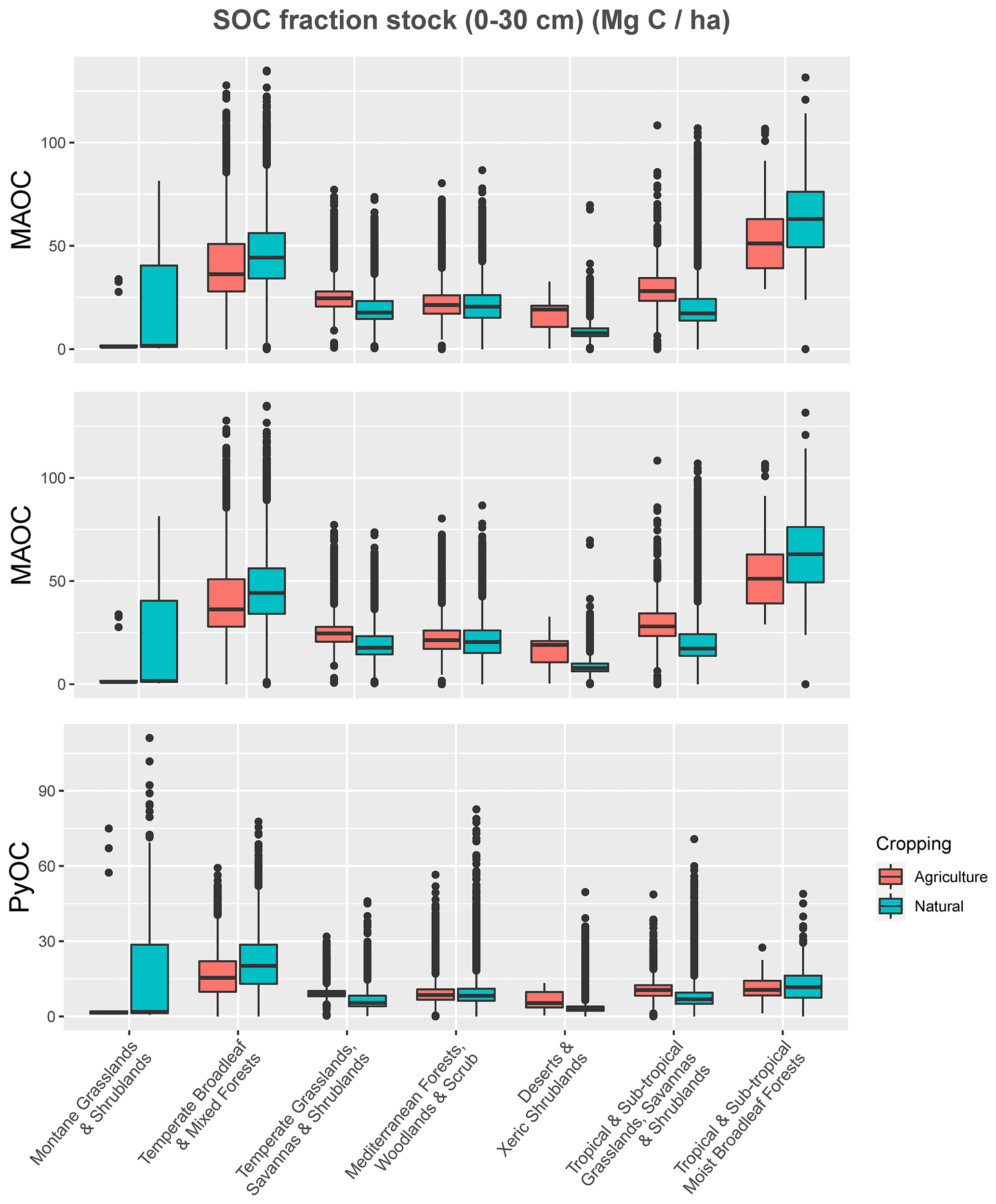
where CF probability_u is the predicted probability and CF mid_u the midpoint of the CF_vol class u. The SOC stock density may be overestimated, especially in soils with a high content of rock fragments, due to using the bulk density of the whole soil and not of fine soil (Poeplau et al., 2017). We then calculated the SOC fraction stocks for the 0–30 cm depth interval using the median predictions of soil thickness (Malone and Searle, 2020) as a constraint in areas with shallow soils (<30 cm). We explored differences among SOC fraction stocks (Mg C ha⁻¹) by biome and land use (natural or agriculture) by taking a regular sample of 500 000 pixels across Australia.

The uncertainty of the SOC fraction density for each GSM depth interval was estimated with simulations. We generated a sample of 500 values from the conditional probability distributions of ilr1 and ilr2 and back-transformed those into proportions of MAOC, POC, and PyOC (percentage of SOC). Similarly, we generated a sample of 500 TOC values with the quantile regression model. To account for the uncertainty of the coarse-fragment volume, we generated a sample of 500 values where (1) the number of samples within each CF_Vol class was proportional to the predicted class probability and (2) assumed a continuous uniform distribution within each class. The sample for bulk density was generated assuming a normal distribution, where the standard deviation was calculated from the prediction interval limits, $\text{sd}=\text{UPL}-\text{LPL}/\mathrm{2}\times z$, with z-score=1.64 for a 90 % prediction interval. We calculated the SOC fraction density for each simulation and calculated the mean and upper and lower prediction interval limits with the 95th and 5th percentiles.

The uncertainty in SOC fraction stocks for 0–30 cm was calculated in a similar way for a sub-set of 98 400 pixels, incorporating the uncertainty of soil thickness (Malone and Searle, 2020). A sample of 500 values for soil thickness was generated assuming a normal distribution, where the standard deviation was calculated from the prediction interval limits (10th and 90th percentiles), $\text{sd}=\text{UPL}-\text{LPL}/\mathrm{2}\times z$, with z-score=1.28 for a 80 % prediction interval. For each sample, we calculated the corresponding thickness for each GlobalSoilMap layer ($j=\mathrm{1},\mathrm{2},\mathrm{3}$) and calculated the SOC fraction stock:

$$\begin{array}{}\text{(18)}& \begin{array}{rl}\text{SOC}& {}_{\text{fraction }i\text{stock}}\left(\mathrm{Mg}\mathrm{C}{\mathrm{ha}}^{-\mathrm{1}}\right)=\\ & \sum _{j=\mathrm{1}}^{\mathrm{3}}{\text{SOC}}_{\text{fraction }i}\left({\displaystyle \frac{{\mathrm{mg}\mathrm{C}}_{\text{SOC fraction }i}}{\mathrm{mg}\mathrm{C}}}\right)\\ & \times \text{TOC}\left({\displaystyle \frac{\mathrm{mg}\mathrm{C}}{\text{g soil}<\mathrm{2}\mathrm{mm}}}\right)\\ & \times {\text{bulk density}}_{\text{whole}}\left({\displaystyle \frac{\text{g soil}}{{\mathrm{cm}}^{\mathrm{3}}}}\right)\\ & \times \left(\mathrm{1}-{\text{Coarse Fragments}}_{\text{vol}}(\mathit{\%}/\mathrm{100})\right)\left({\displaystyle \frac{\text{soil}<\mathrm{2}\mathrm{mm}}{\text{g soil}}}\right)\\ & \times {\text{thickness}}_j\left(\mathrm{cm}\right)\\ & \times \text{correction units}\left({\displaystyle \frac{{\mathrm{10}}^{\mathrm{8}}{\mathrm{cm}}^{\mathrm{2}}}{\mathrm{ha}}}{\displaystyle \frac{\mathrm{Mg}}{{\mathrm{10}}^{\mathrm{9}}\mathrm{mg}}}\right).\end{array}\end{array}$$

The 95th and 5th percentiles of the 500 simulations were calculated to estimate the upper and lower prediction interval limits of the SOC fraction stocks. The means of the 500 simulations were compared with predictions of SOC fraction stocks for 0–30 cm at those locations by Viscarra Rossel et al. (2019).

We performed a variance-based, global sensitivity analysis of every pixel to identify which variables account most for the uncertainty of SOC fraction density and stocks and how they vary spatially. We calculated the first-order and total effects of Sobol's sensitivity indices (Saltelli et al., 2008). The first-order sensitivity index S_i represents the main effect contribution of each input factor X_i (SOC fraction %, TOC, CF_vol, and bulk density) to the variance of the output of model Y (SOC fraction density). It is calculated as the quotient between the variance of the conditional expectation of the output with respect to an input factor and the unconditional variance of the output (Saltelli et al., 2008). S_i ranges between 0 and 1, and a high value indicates that factor X_i is an important contributor to the variance of the output (if we knew the true value of X_i, we would significantly reduce the variance of Y). The total effect index S_Ti includes non-additive features of the model by accounting for the first-order effect of X_i and its interactions with other factors on the variance of Y. When S_Ti is close to 0, the factor is non-influential on the model output variance. A comprehensive explanation of the variance-based methods for global sensitivity analyses can be found in Saltelli et al. (2008). We calculated the indices with the method by Martinez (2011) with the function sobolmartinez of the sensitivity package in R (Iooss et al., 2021).

3 Results

3.1 Variation of the proportions of SOC fractions with depth and biome

The boxplots of the SOC fraction data predicted with spectral models showed that most of the TOC was found in the MAOC fraction with a mean (± standard deviation) of 59 % ± 16 %, whereas 28 % ± 18 % of TOC was PyOC and 13 % ± 11 % was POC. The allocation of TOC to the MAOC fractions increased with depth (Fig. 4), with means (± standard deviation) of 56 % ± 17 %, 59 % ± 17 %, and 62 % ± 18 % at 0–5, 5–15, and 15–30 cm, respectively. Conversely, the proportion of SOC stored as POC decreased with depth, from 15 % ± 11 % and 13 % ± 11 % in the top 0–5 and 5–15 cm to 11 % ± 11 % at 15–30 cm. The percentage of SOC in the PyOC fraction remained relatively constant with depth, with values around 29 % ± 17 % (Fig. 4). Hence, on average, carbon vulnerability decreased slightly with depth, with Vp=0.2 ± 0.2 at 0–5 and 5–15 cm and Vp=0.1 ± 0.3 at 15–30 cm.

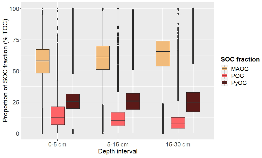
Figure 4 Distribution of TOC among three SOC fractions in the spectral dataset: MAOC, POC, and PyOC.

The distribution of TOC among fractions showed similar patterns across biomes ($\text{MAOC}\gg \text{PyOC}>\text{POC}$), except for montane grasslands and shrublands, where 67 % of TOC was stored as PyOC, while only 27 % was stored as MAOC (Table 2 and Fig. S2 in the Supplement). However, there were only 160 observations located in this biome. The proportion of TOC as POC was greater in Mediterranean forests and scrub, temperate forests, and tropical and sub-tropical forests. In Mediterranean systems, the proportion of MAOC was around 10 % less than across the other biomes, (excluding montane grasslands), whereas the smallest proportion of PyOC was found in tropical and sub-tropical forests. Hence, the Vp was highest in the Mediterranean biome, followed by temperate forests and tropical and sub-tropical forests, decreasing with depth across all biomes (Table 2).

Table 2 Summary statistics, mean (± standard deviation) of SOC fractions, and Vp by biome. Spectral dataset used as input for digital soil mapping. N: number of observations. MAOC, POC, and PyOC.

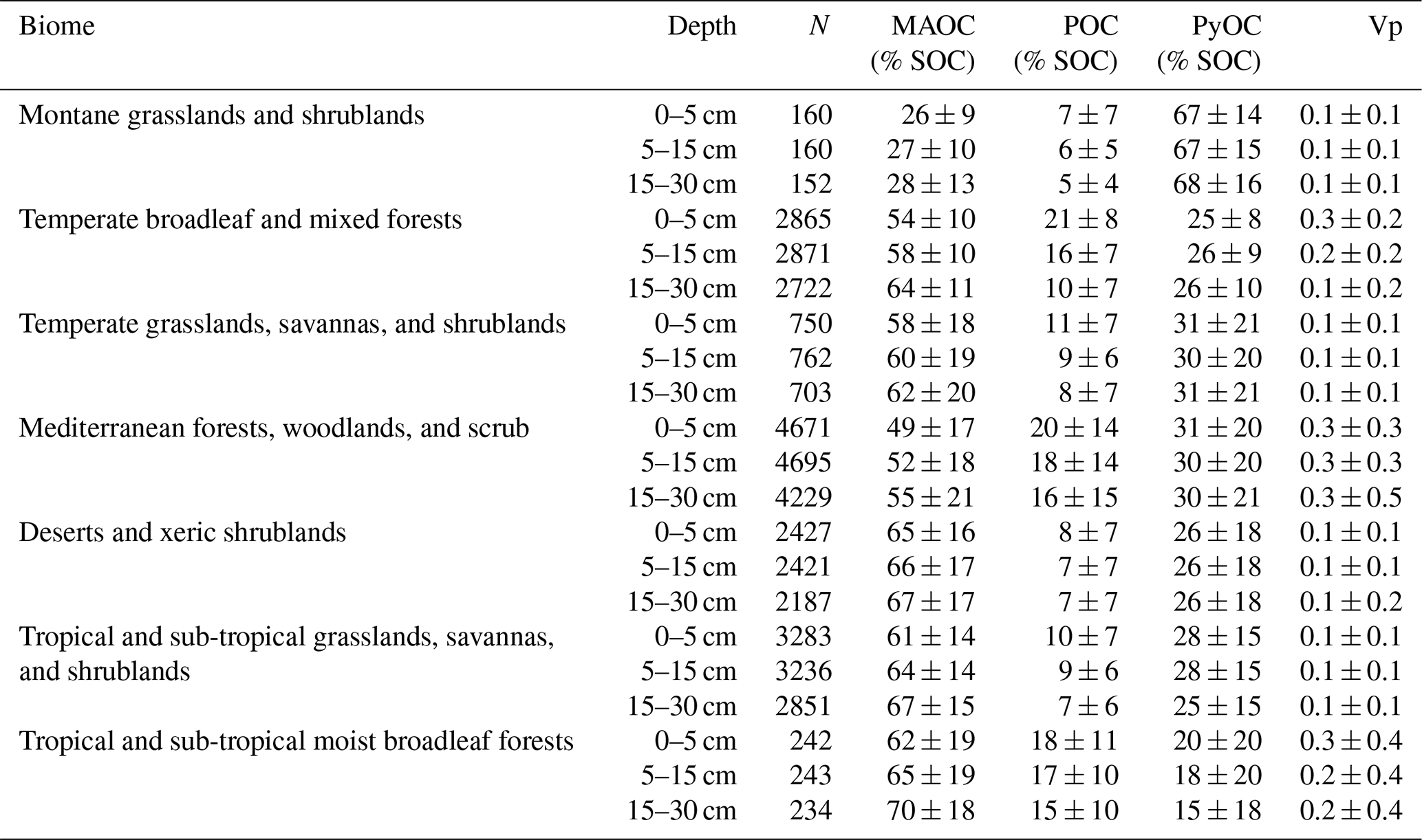
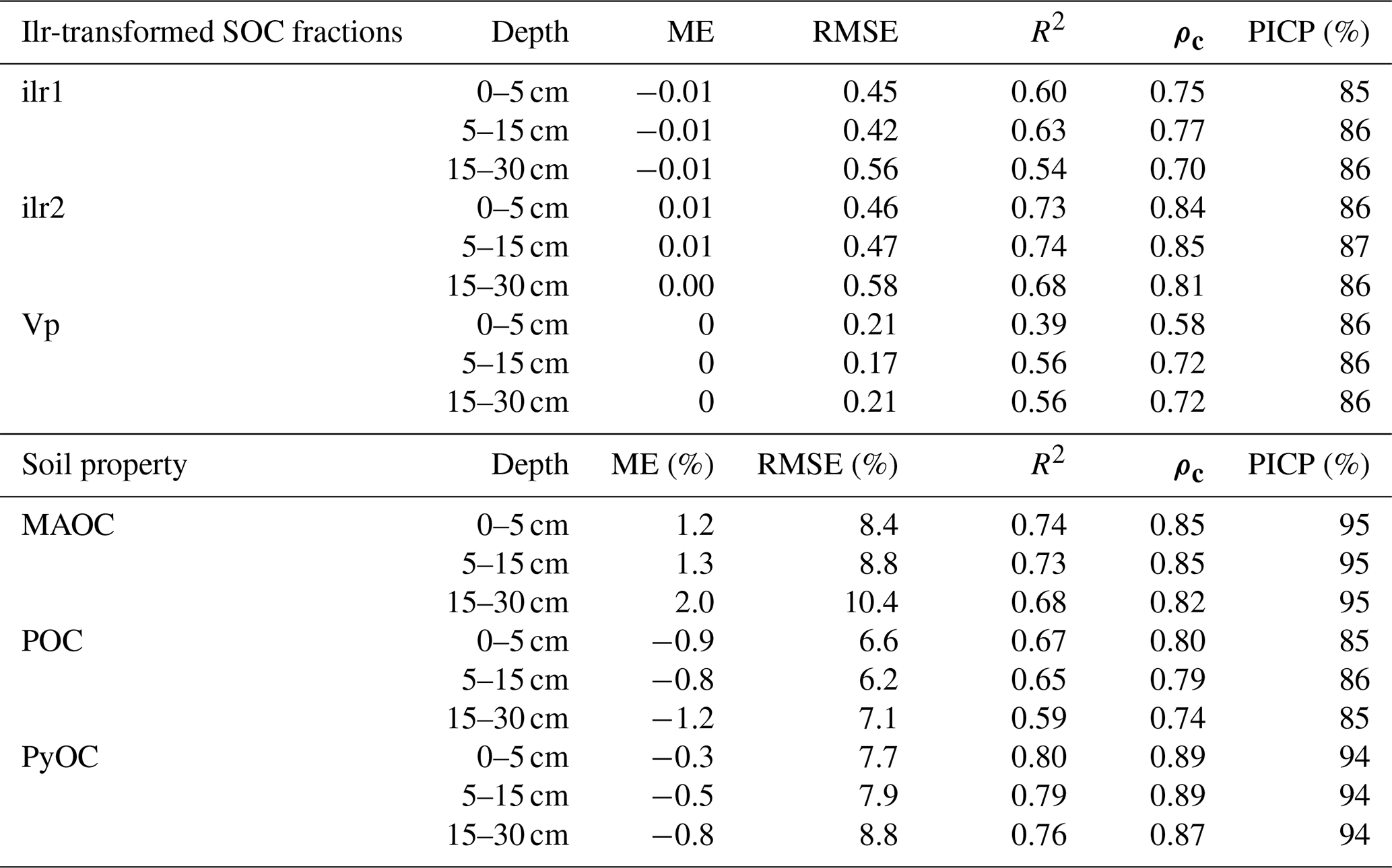
Table 3 Cross-validation statistics for ilr1, ilr2, MAOC, POC, PyOC, and Vp by depth interval. ME, RMSE, R², Lin's concordance correlation coefficient (ρ_c), and PICP.

3.2 Cross-validation statistics for SOC fractions

The cross-validation statistics indicated that both ilr-fraction models had a similar RMSE and bias, although the R² and ρ_c were better for ilr2 than ilr1. Model performance indices decreased with depth but were overall good, with R²≥0.54 for ilr1 and R²≥0.68 for ilr2. Similarly, the concordance coefficients indicated good agreement between predictions and observations, with ρ_c≥0.70 for ilr1 and ρ_c≥0.81 for ilr2. The uncertainty was somewhat underestimated (Table 3) but was close to a PICP of 90 %. The cross-validation of the back-transformed SOC fractions indicated that the concordance coefficient and R² followed the trend $\text{PyOC}>\text{MAOC}>\text{POC}$ (Table 3). In contrast, the RMSE was greatest for MAOC, with values between 8 % and 10 %, and was somewhat smaller for PyOC and POC, between 8 % and 6 %. SOC fraction predictions had a small bias, with an average underprediction of MAOC and an overprediction of POC and PyOC. The accuracy plots (Fig. S3 in the Supplement) indicate that the uncertainty was overestimated for MAOC and PyOC and underestimated for POC, for all probability intervals, although the uncertainty was adequately estimated for the 90 % prediction interval (Table 3). Cross-validation statistics for SOC vulnerability were worse than for the SOC fractions, with R² ranging between 0.39 and 0.56 and a concordance coefficient between 0.58 and 0.72, which is possibly due to some extreme values in the calibration dataset. A PICP around 86 % indicates that the uncertainty was somewhat underestimated.

3.3 Cross-validation statistics for coarse-fragment classes

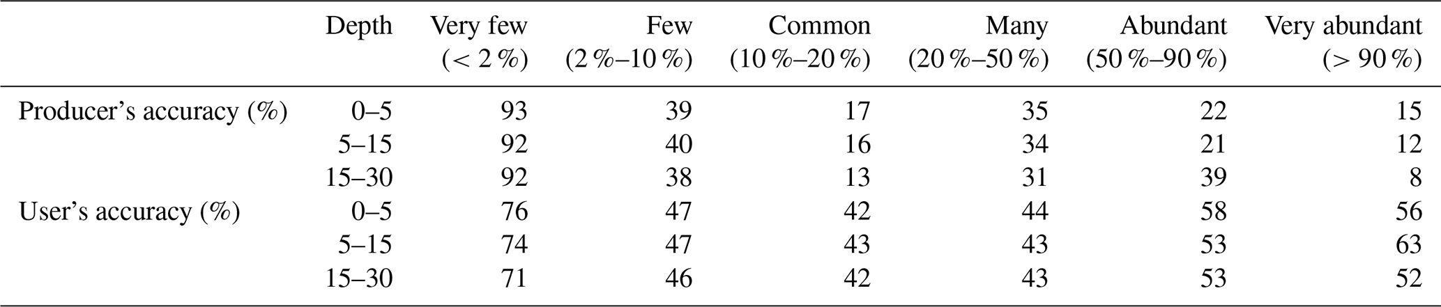
The overall accuracy of predicting coarse-fragment classes was 67 % for the 0–5 cm depth interval, 66 % for the 5–15 cm depth interval, and 63 % for the 15–30 cm depth interval. The kappa statistics were 0.39, 0.38, and 0.37, respectively, which indicate some agreement. The producer's accuracy was around 90 % for the “very few” class across the three depths, but the omission error was significant for the remaining classes, especially for “common” and “very abundant”, with values around 15 %. The user's accuracy was smaller than 50 % for the classes “few”, “common”, and “many” coarse fragments but improved somewhat for “very abundant”, “abundant”, and “few” (Table 4). The confusion matrices are provided in the Supplement (Tables S1–S3).

Table 4 Cross-validation statistics for classification of coarse fragments (% vol).

3.4 Variable importance for predicting proportions of SOC fractions and coarse fragments

The environmental covariates important for both the ilr1 and ilr2 models were parent material and climate, whereas relief and organisms were secondary factors (Fig. 5). The rank of the 10 most important variables indicates that parent material, soil properties, and relief were more relevant for ilr1, especially gravity, gamma radiometrics K, clay, and elevation (DEM), whereas for ilr2 the importance of gamma radiometric variables and gravity was more important for the depth intervals 5–15 and 15–30 cm. By contrast, climate variables were more critical for ilr2 models, especially precipitation seasonality (PTS1 and PTS2), potential evaporation (EPA and EPX), and annual temperature (TNM and TXM), while the annual temperature range (TRA) was more important for the ilr1 model. Amongst the relief covariates, DEM, topographic wetness index (TWI), and roughness were the most relevant variables for both ilr1 and ilr2. Non-photosynthetic vegetation and mean EVI were the only covariates representing the soil-forming factor organisms with some importance in the models. The most significant variables predicting the distribution of coarse fragments were gamma radiometrics and other proxies of parent material (Th, U, total dose, and ratio $\mathrm{Th}/\mathrm{K}$), followed by some covariates of climate (EPX, TRA) and relief (roughness, slope, DEM) (Fig. 6).

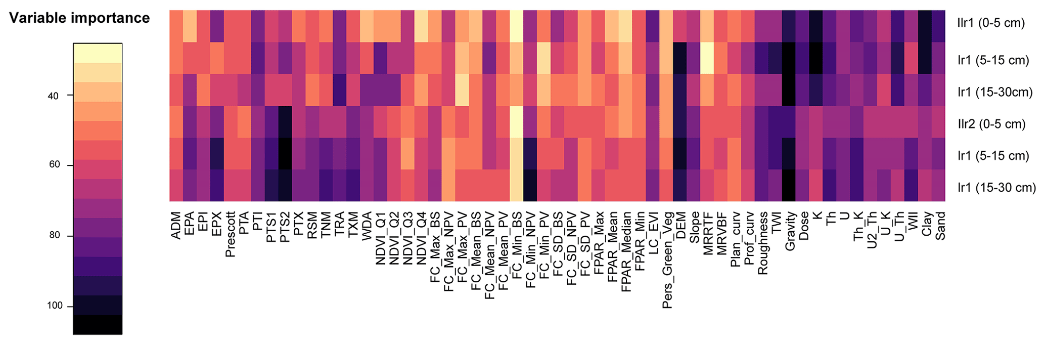
Figure 5 Variable importance of random forest models for predicting ilr-transformed SOC fractions. Variable importance was calculated from permutation as per Breiman (2001).

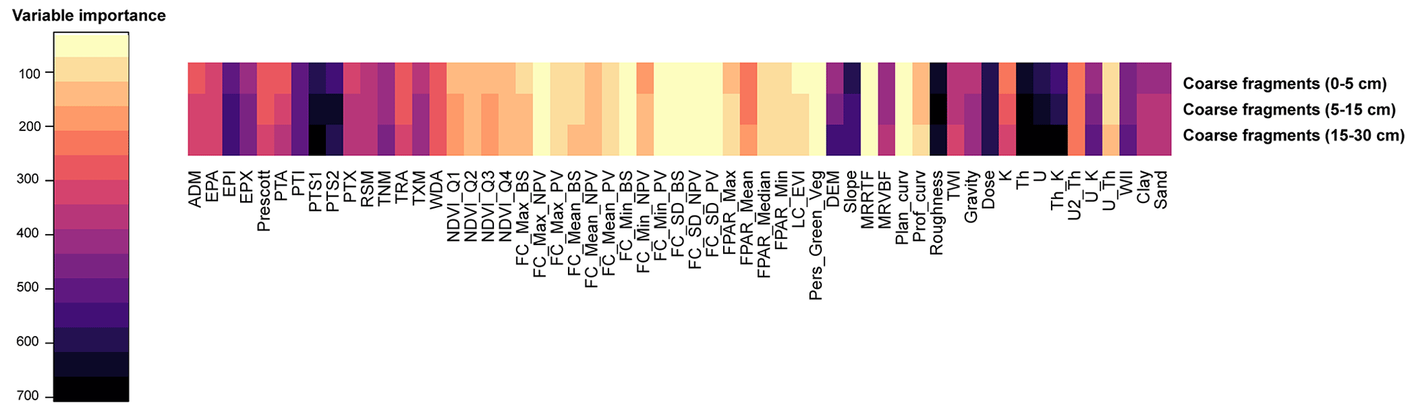
Figure 6 Variable importance of random forest probability models for coarse-fragment classes. Variable importance was estimated with Gini index impurity (Sandri and Zuccolotto, 2008).

3.5 Maps of SOC fraction proportions, SOC vulnerability, and coarse fragments

The spatial predictions of SOC fractions allocated most of the SOC to the MAOC fraction across most of Australia (Fig. 7a and Figs. S4–S6 in the Supplement). The POC proportion was greater in the Mediterranean and temperate areas along the coast and northern Queensland. There were three main regions with a high proportion of PyOC: in the north-west around the Prince Regent River and the Dampier Peninsula, in the west south of the Gascoyne River, and in some parts of the south and centre, e.g. east of Lake Frome. These predictions are likely driven by some calibration data with high PyOC values at these locations (Fig. 2). The prediction intervals for the SOC fractions were wide (Figs. S4–S6) but, based on the accuracy plots (Fig. S3), were estimated relatively well at the 90 % confidence level. Therefore, SOC vulnerability was higher in areas with Mediterranean and temperate climates and in the centre and east (Fig. 7b). The latter is likely an artifact since that area is largely occupied by salt lakes (Kati-Thanda/Lake Eyre) and the Strzelecki Desert. The coarse-fragment class with the highest probability across Australia was “very few” (<2 %), and the estimated volume of coarse fragments was higher in western and north-western Australia as well as along the Great Divide (Figs. S7–S9 in the Supplement).

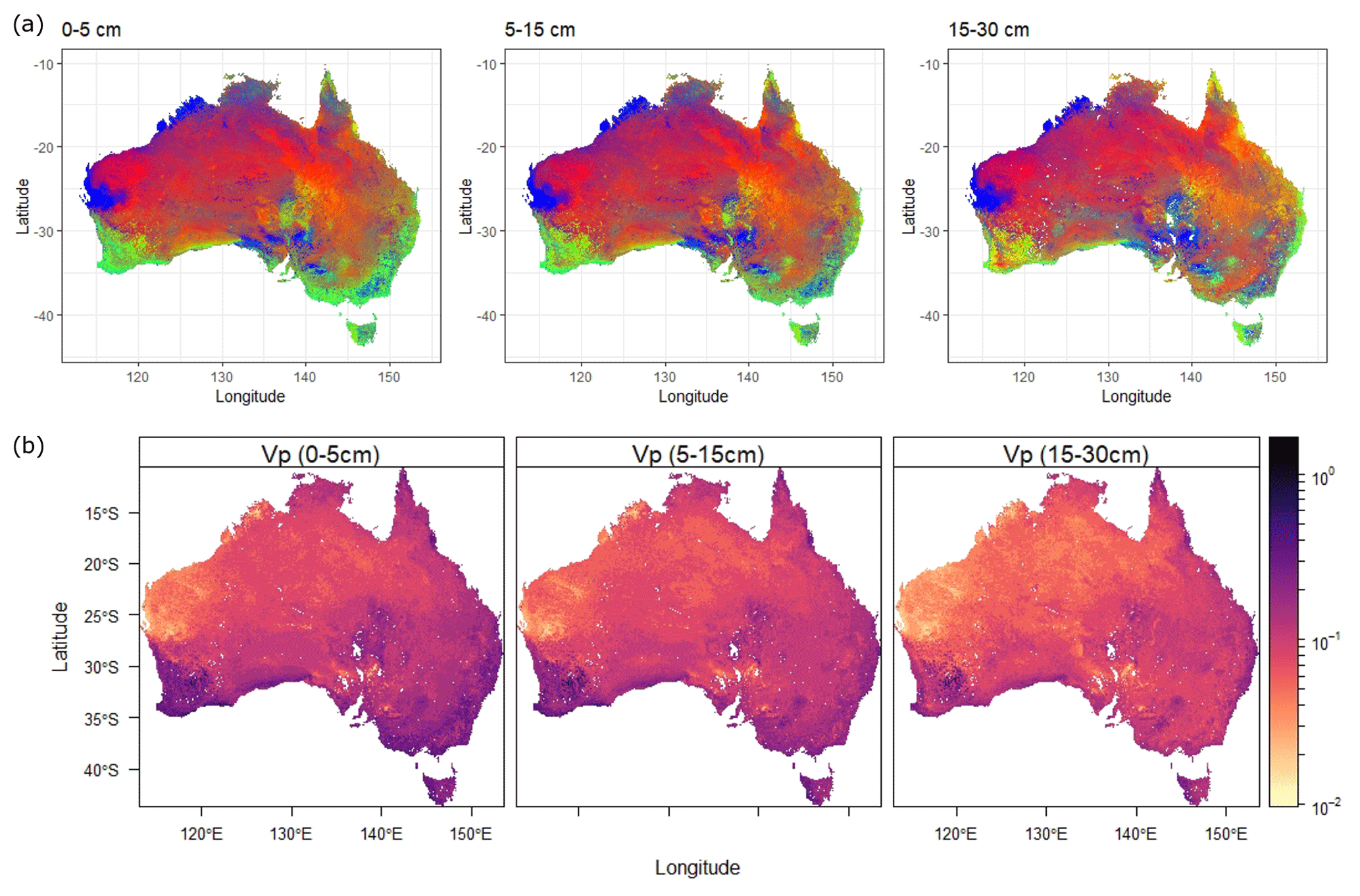
Figure 7 (a) Composite of the contributions of the three SOC fractions to SOC for the depth intervals 0–5, 5–15, and 15–30 cm. The colours indicate the dominant fractions with MAOC in red, POC in green, and PyOC in blue. (b) SOC vulnerability for the three depth intervals. SOC vulnerability is in the log10 scale for better differentiation.

3.6 SOC fraction stocks and sensitivity analysis

The spatial patterns of SOC fraction density are mainly determined by the spatial gradient in TOC concentration. Thus, irrespective of the dominant fraction, SOC density follows a climatic gradient and is higher in the south-west, east, Tasmania, and some regions in northern Australia (Figs. S10–S12 in the Supplement). PyOC density was predicted to be higher along the Snowy Mountains, as the proportion of PyOC in montane grasslands and shrublands in the calibration dataset was around 67 % (Table 2) and the TOC concentration was high (Fig. S10). POC density was higher in south-western Australia, east of Tasmania, and in the south-east and east. MAOC density showed similar patterns and had higher values than POC. Ultimately, the SOC fraction stocks at 0–30 cm (Fig. 8) were not high in the east of Tasmania because these are organic soils, and the median soil thickness was estimated for mineral soils. Similarly, the SOC stocks in the Snowy Mountains were constrained by the shallow soil thickness. The total stocks of SOC fractions for Australia (0–30 cm) were 13 Pg MAOC, 2 Pg POC, and 5 Pg PyOC. The predictions of SOC fraction stocks were generally smaller but correlated with the previous SOC fraction stocks estimated by Viscarra Rossel et al. (2019) (Figs. S21 and S22 in the Supplement). The Pearson correlation coefficients were, respectively, r=0.72 for MAOC, r=0.75 for POC, and r=0.77 for PyOC (Fig. S21). The differences between the predictions of the present study and Viscarra Rossel et al. (2019) were higher in areas of shallow soils (Fig. S22). We mapped the uncertainty of the SOC fraction density (mg C cm⁻³) by depth interval with simulations (Figs. S11–S13 in the Supplement) and estimated the uncertainty in SOC fraction stocks (0–30 cm) in a sub-set of pixels (Fig. 9).

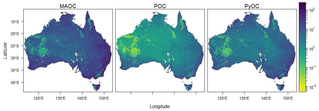
Figure 8 SOC fraction stocks (0–30 cm) (Mg C ha⁻¹). The values are represented in the log10 scale.

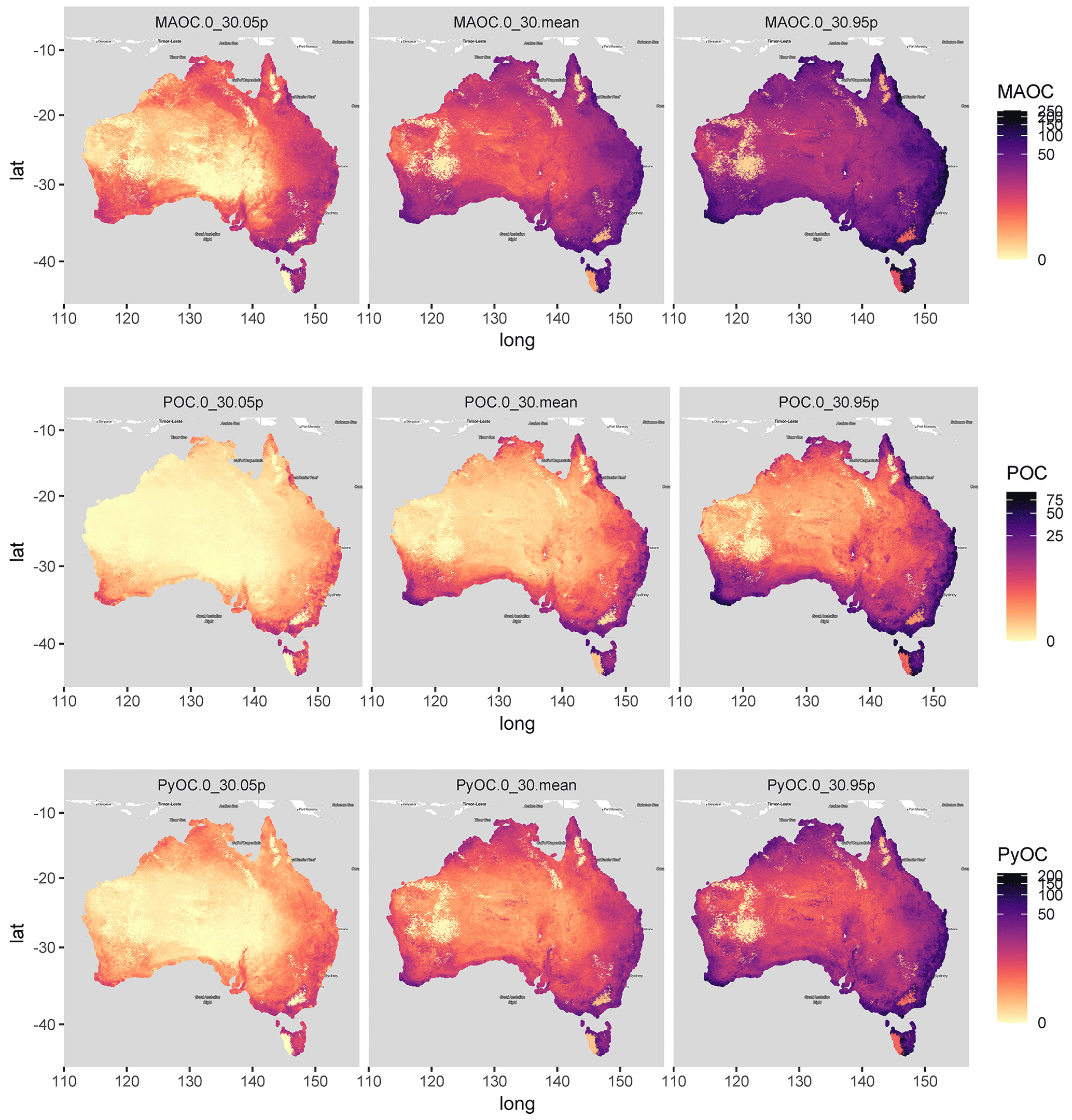
Figure 9 Uncertainty of SOC fraction stocks (Mg C ha⁻¹) for 0–30 cm calculated with 500 simulations in a sub-set of 98 400 pixels.

MAOC stocks were generally higher in tropical and sub-tropical moist broadleaf forests and temperate broadleaf and mixed forests (Fig. 10). In some biomes (temperate and tropical grasslands, savannas and shrublands, and desert and xeric shrublands), MAOC stocks were higher in agricultural soils (which included rainfed and irrigated pastures) than in natural areas. In the Mediterranean biome, MAOC stocks were similar in natural and agricultural regions, where only 1.6 % of the agricultural area (pastures and cropping) is irrigated (Australian Bureau of Agricultural and Resource Economics and Sciences, 2022). POC stocks followed similar trends to MAOC, although in the Mediterranean biome, POC was greater in agricultural soils than in natural areas. Montane grasslands and shrublands had maximum values of PyOC, although the median PyOC stocks were greater in the natural and agricultural temperate biomes, followed by tropical and sub-tropical forests (Fig. 10).

Figure 10 SOC fraction stock (Mg C ha⁻¹) by biome and land use. MAOC, POC, and PyOC.

The two variables with the most influence on the uncertainty of SOC fraction density were TOC concentration and SOC fraction percentage (Figs. S14–S19 in the Supplement). The total Sobol indices varied spatially depending on the SOC fraction, with TOC being the most relevant in interior areas with smaller SOC stocks and both variables having a similar influence towards the coast in the southern half of the continent. Total Sobol indices show that bulk density was not very influential on the uncertainty of the SOC fraction density. This may be related to the relatively small prediction interval of the bulk-density maps, calculated with bootstrapping (Viscarra Rossel et al., 2015). Coarse fragments also had a small influence, as indicated by the small Sobol indices across most of Australia, except in zones where a higher volume of coarse fragments had a higher probability, e.g. western and northern Australia (Figs. S7–S9). A sensitivity analysis was also performed for the total SOC fraction stocks (0–30 cm) at a sub-set of pixels to determine the influence of soil thickness on the uncertainty. The results of the first and total Sobol indices indicate that soil thickness had a high influence on the SOC fraction stocks in areas of shallow soils, since we only estimated the stocks for 0–30 cm (Fig. S20 in the Supplement). The variables with higher total Sobol indices for SOC fraction stocks were generally TOC concentration and the distribution among SOC fractions at 5–15 and 15–30 cm.

4 Discussion

4.1 Differences in SOC allocation to fractions across biomes

The trend of lower MAOC proportions with increasing sand content was observed across all biomes (Fig. 11). Sand content is generally higher in the western half of Australia, coinciding with the Mediterranean and desert biomes, which have a mean (± standard deviation) sand content of 73 % ± 14 % and 71 % ± 10 %, respectively, in the calibration dataset. The smaller capacity of coarse-textured soils to stabilise SOC through organo–mineral associations may partly cause the lower proportion of MAOC and higher POC in Mediterranean soils (Figs. 10 and 11). Similarly, Doetterl et al. (2015b) found that more SOC was stored as POC in arid environments, where biochemical weathering is limited, due to a lower capacity for physico-chemical protection.

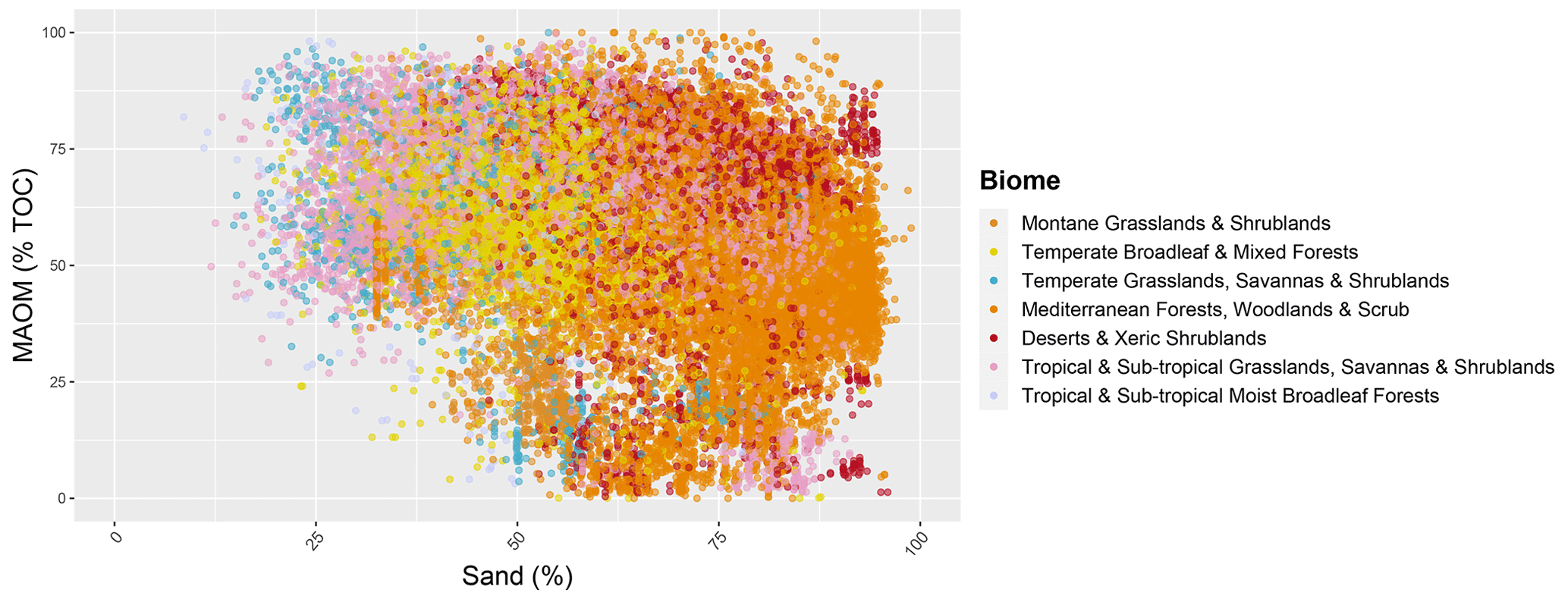
Figure 11 Allocation of SOC to the MAOC plotted vs. sand content (%) by biome, from calibration data.

Conversely, the proportion of SOC found as MAOC is around 60 % in Australian temperate grasslands, savannas, and shrublands, 50 % in Mediterranean forests and woodlands, ∼54 %–64 % in temperate forests, and 60 %–70 % in tropical ecosystems (Table 2). Sokol et al. (2022) reported that a high proportion of MAOC in temperate grasslands (∼70 %) was due to higher net primary productivity (NPP) and microbial decomposition favouring MAOC formation. They also found that savannas and temperate and tropical forests had a relatively high proportion of MAOC (∼64 %), whereas shrublands had a lower proportion of MAOC (∼42 %). Some differences are possibly explained by a higher percentage of SOC as PyOC in some systems (e.g. montane grasslands, tropical and sub-tropical savannas), in comparison to two fractions (MAOC and POC) (Sokol et al., 2022), and differences in the definitions of biomes.

4.2 Abiotic and biotic predictors of SOC allocation to SOC fractions at the continental scale

Climate and parent material were the main soil-forming factors for predicting the partitioning of SOC into fractions in continental Australia. Climate is a major driver of SOC storage (Wiesmeier et al., 2019) and partitions into SOC fractions at the continental scale (Bui et al., 2009). Climate influences weathering of primary minerals, the development of reactive secondary minerals over long-term pedogenetic processes, and the chemistry of the soil solution, which in turn condition the formation of organo–mineral associations (Kleber et al., 2015). At the same time, climate also controls SOC decomposition rates and input of organic matter through net primary productivity. At the global scale, climate is a major driver of the abundance, persistence, and distribution of SOC among fractions (Heckman et al., 2022), with different effects by fractions and depth. Mean annual temperature had a strong effect on POC. The content of free POC decreased with an increase in MAT in topsoils (0–30 cm), whereas free POC increased slightly with MAT in subsoils, and occluded POC increased with MAT at all depths. In contrast, the wetness index (ratio of annual precipitation to potential evapotranspiration) had a stronger effect on MAOC, suggesting that, under wetter conditions, weathering and increasing reactivity of minerals with depth, together with the downward transport of organic matter, enhance the formation of organo–mineral associations (Kleber et al., 2015). Parent material alone did not have a significant effect on the partitioning of SOC into MAOC at the global scale but on interaction with the wetness index (Heckman et al., 2022).

In this study we could not verify the influence of soil geochemistry and mineralogy (metal ions, sesquioxides) on the proportion of SOC fractions due to a lack of samples with extensive laboratory analysis. Soil geochemical properties have been found to control SOC storage at continental and regional scales (Doetterl et al., 2015b) and are involved in the stabilisation of SOC, with different mechanisms depending on the climatic context and soil pH (von Lützow et al., 2006; Rasmussen et al., 2018). In Australia, soil physico-chemical properties, and particularly extractable iron, were the most important predictors of SOC storage at the continental scale (Li et al., 2020). Multiple soil chemical properties can be estimated fairly well with mid-infrared spectral models (Ng et al., 2022). Therefore, future research could expand on this study by investigating the relationships (and their spatial patterns) between soil chemical properties (exchangeable Ca and Mg, oxalate- and dithionite-extractable Fe and Al) and MAOC in the context of Australia, where the soil pH is quite acidic even under arid and semi-arid conditions.

Among vegetation variables, only EVI and the fractional cover of non-photosynthetic vegetation were important predictors for the distribution of SOC among fractions. The fraction of non-photosynthetic vegetation may be indicative of the type of C input into the soil (e.g. woody debris), which influences the subsequent decomposition and transformation pathways of organic matter (Cotrufo et al., 2015) and the allocation to SOC fractions (Heckman et al., 2022).

4.3 Vulnerability of SOC fractions to climate change

We estimated the total stock of SOC fractions for Australia (0–30 cm) in 13 Pg MAOC, 2 Pg POC, and 5 Pg PyOC, which give a total of 20 Pg SOC. This value is smaller than a previous baseline of SOC stock of 25 Pg SOC for Australian topsoils but is within its prediction interval (19–31.8 Pg C) (Viscarra Rossel et al., 2014). Differences in the total SOC stock may be partly due to differences in soil thickness (Fig. S22) and in TOC predictions between the previous version of SLGA v1 (Viscarra Rossel et al., 2015, 2014) and the current SLGA v1.2 (Wadoux et al., 2022). Both maps show similar patterns and ranges of TOC values, and hence differences in SOC fraction and total SOC stock may be mostly caused by differences in the DSM framework (e.g. calculating SOC fraction densities prior to spatialisation, accounting or not for coarse fragments) and input soil layers (soil thickness).

Our calculations estimated that about 64 % of the total SOC is stored as mineral-associated SOC, which is consistent with other studies at global and continental scales (Heckman et al., 2022). In Australian topsoils, we estimated that only 10 % of the SOC stock is stored as POC and 26 % as PyOC. POC is generally more responsive than MAOC to management practices and to global change (Rocci et al., 2021). Our PyOC estimate is higher than the world average (14 % of SOC, Reisser et al., 2016) but is consistent with a study in Australia (14 %–33 %, Lehmann et al., 2008). Since the 1970s, there has been an upward trend in “fire weather” conditions in Australia linked to anthropogenic climate change (Harris and Lucas, 2019), which may modify the proportion and stock of PyOC.

There is great uncertainty about the effects of an increase in temperature on SOC fraction stocks and dynamics. There is much evidence supporting the temperature sensitivity of decomposition being higher for stable SOC fractions (Conant et al., 2008; Jia et al., 2020) or SOC pools with longer mean residence times (Li et al., 2013), although other studies indicate no differences or opposite trends in sensitivity between SOC fractions (von Lützow and Kögel-Knabner, 2009). Since most SOC is stored as MAOC, an increase in MAOC decomposition rates with temperature (when soil moisture is not limiting) may turn some soils into a C source (Li et al., 2013). By contrast, coarse-textured soils with a lower capacity for physico-chemical protection and a greater proportion of POC may be more vulnerable to SOC loss with an increase in temperature than fine-textured soils (Hartley et al., 2021). Heckman et al. (2022) found a decrease in SOC persistence among all SOC fractions, with a higher mean annual temperature at the global scale and a decrease in SOC abundance in free POC in the surface (0–30 cm). However, the increase in temperature did not affect the abundance of occluded POC and MAOC, which may be less vulnerable to warming. Similarly, a recent meta-analysis (Rocci et al., 2021) found a reduction in POC (% SOC) with warming, suggesting that soils with higher POC contributions may be more vulnerable to SOC loss. In the case of Australia, this would mean that coarse-textured soils from Mediterranean and temperate ecosystems may be more vulnerable to an increase in temperature.

Other climatic and hydrological conditions linked to climate change may also affect SOC fraction stocks in Australia. Changes in the precipitation regime (e.g. intensity and frequency of droughts, extreme precipitation events and flooding) can affect the SOC fraction stocks by either limiting or enhancing C input into the soil (effects on NPP) and modifying decomposition or SOC losses by increased erosion. Rocci et al. (2021) did not find clear effects on the partitioning of SOC among fractions with an increase in precipitation, although they found a negative tendency for POC and a positive tendency for MAOC. The effect of wind erosion on SOC loss will depend on particle-size distribution and soil cover, with vulnerable soils losing 3.6 Mg C ha⁻¹ in south-western Australia (Harper et al., 2010). While wind erosion may deplete locally the soil of clay- and silt-sized particles and light SOC fractions (light MAOC and light POC) and facilitate mineralisation by disruption of aggregates, aeolian transport and deposition may contribute to SOC enrichment in other regions (Webb et al., 2012). The influence of water erosion on SOC fractions will vary with agricultural practices, with the latter sometimes having a stronger effect on POC than erosion depending on hillslope position (Zhao et al., 2022). SOC destabilisation and stabilisation processes vary along the hillslope with changes in particle-size distribution, degree of weathering, and abundance of secondary minerals (Doetterl et al., 2015a).

4.4 Components in the calculation of SOC fraction stocks: current limitations and priorities for improving their quantification

The maps of total Sobol indices inform which variables are more influential on the uncertainty of SOC fraction densities and stocks across Australia and can guide the priorities for mapping locally, regionally, or at a continental scale the different components of SOC fraction stocks. TOC was generally the main variable of influence for SOC fraction density and stocks, and methods for measuring it efficiently and more economically on farms and in the laboratory are experiencing continuous development. TOC concentration in Australian ecosystems has been underestimated by previous SOC maps in temperate forests (Bennett et al., 2020). It is then possible that in this study the SOC fraction stocks for these ecosystems are underestimated for two reasons: random forest models tend to underestimate the high values (Wadoux et al., 2022), and the SOC fraction data used to calibrate the spectral models did not represent forest ecosystems.

The percentage of TOC in the three fractions was generally the second variable of influence on the uncertainty of SOC fraction density. Still, it could be the most influential variable in areas with moderate to low SOC density. Soil thickness was the most influential variable on SOC fraction uncertainty in areas of shallow soils.

Several sources of error in the SOC fraction predictions were not accounted for in the sensitivity analysis, like the error propagated from the fractionation scheme, the different spectral models, digital soil mapping models, or the fact that the fractionation in the original dataset was applied to agricultural soils and some pastures but lacks forest soils. There is also an underrepresentation of some biomes and land cover types (e.g. tropical savannas) in the soil samples used for fractionation, which decreases the reliability of the SOC fraction stock predictions in some areas. Ideally, the spectral models could be improved by increasing the representation of different natural ecosystems (especially forests and woodlands) across biomes, which may have very different mechanisms of stabilisation.

Another limitation of the current study is linked to the fractionation method used for the determination of PyOC. ¹³C NMR has been used in the past to determine the ROC in the soil (Baldock et al., 2013c). ROC has a chemical composition that is not incompatible with that of charcoal (or that is dominated in its majority by charcoal and charred plant residuals), but there is a potential presence of other poly-aryl carbon compounds that do not have a pyrogenic origin. However, the benzene polycarboxylic acid (BPCA) approach is a preferred method that gives a more realistic estimate of concentrations of PyOC in soil. Hence, future studies could carry a comparison between PyOC determined with BCPA and ¹³C NMR in Australian soil samples (Dymov et al., 2021).

We used estimates of rock fragment volume in the calculation of SOC fraction stocks, which can overestimate the stocks when the bulk density is for the whole soil instead of that for the fine soil (<2 mm) (Poeplau et al., 2017). The error due to combining volumetric coarse fragments and the bulk density of the whole soil is not captured in the sensitivity analysis. Neglecting the content of coarse fragments can significantly overestimate the SOC fraction stocks in soils with non-negligible stoniness (>5 %), more than doubling the actual stocks in soils with >30 % rock fragments (Poeplau et al., 2017). We anticipated that the inaccuracy of the coarse-fragment maps and the broad range within each category would contribute significantly to the error and uncertainty in the SOC fraction stock estimates. This was true in areas with non-negligible stoniness (>2 %), as indicated by the total Sobol indices (Figs. S14–S19). However, compared with the distribution among SOC fractions and TOC concentrations, coarse fragments were not the most relevant variable influencing SOC fraction density.

5 Conclusions

SOC fractions are crucial as input for dynamic SOC models. These maps of MAOC, POC, and PyOC can be used as input for modelling SOC stocks under different management strategies and identify areas where SOC stocks could be augmented more efficiently (i.e. areas with higher SOC sequestration potential/SOC deficit) (Meyer et al., 2017; Martin et al., 2021). Land management practitioners could then optimise the spatial allocation of different agricultural practices while maintaining several soil functions and services, mainly food security and climate change mitigation and adaptation.

The main covariates predicting the distribution of SOC among fractions at the continental scale were identified as climate and parent material. However, a comprehensive and homogeneous dataset that examines the soil geochemical properties (e.g. exchangeable Ca and Mg, extractable Fe and Al, CEC ascribed to minerals) controlling SOC stabilisation processes is lacking in Australia. The diversity of climatic and pedological conditions suggests that different mechanisms will control SOC stabilisation and dynamics across the continent, as observed in other regions (Rasmussen et al., 2018). The link between mycorrhizal associations (Averill et al., 2014; Jo et al., 2019) and soil microbial community composition (e.g. N₂-fixing organisms), soil stoichiometry and vegetation communities (Bui and Henderson, 2013), and their effects on SOC fractions (Cotrufo et al., 2019) should be further investigated. For example, it is possible that in native ecosystems with a higher soil C:N ratio and recalcitrant litter, there may be a high proportion of SOC as POC, whereas the MAOC fraction may not be C-saturated.

The uncertainty in the spatial predictions of SOC fraction stocks was driven mainly by TOC and the proportion of SOC fraction predictions, which in turn rely on spectral predictive models developed with soil samples originating mainly from agricultural soils. However, the sensitivity analysis allows targeting of variables that should be prioritised at the local and regional scales to reduce the uncertainties of SOC fraction stock estimates. Future works will include more sampling efforts for measuring TOC, fractionation on underrepresented regions, or development of local spectral models for predicting SOC fractions.