Impacts and uncertainties of climate-induced changes in watershed inputs on estuarine hypoxia

Multiple climate-driven stressors, including warming and increased nutrient delivery, are exacerbating hypoxia in coastal marine environments. Within coastal watersheds, environmental managers are particularly interested in climate impacts on terrestrial processes, which may undermine the efficacy of management actions designed to reduce eutrophication and consequent low-oxygen conditions in receiving coastal waters. However, substantial uncertainty accompanies the application of Earth system model (ESM) projections to a regional modeling framework when quantifying future changes to estuarine hypoxia due to climate change. In this study, two downscaling methods are applied to multiple ESMs and used to force two independent watershed models for Chesapeake Bay, a large coastal-plain estuary of the eastern United States. The projected watershed changes are then used to force a coupled 3-D hydrodynamic–biogeochemical estuarine model to project climate impacts on hypoxia, with particular emphasis on projection uncertainties. Results indicate that all three factors (ESM, downscaling method, and watershed model) are found to contribute substantially to the uncertainty associated with future hypoxia, with the choice of ESM being the largest contributor. Overall, in the absence of management actions, there is a high likelihood that climate change impacts on the watershed will expand low-oxygen conditions by 2050 relative to a 1990s baseline period; however, the projected increase in hypoxia is quite small (4 %) because only climate-induced changes in watershed inputs are considered and not those on the estuary itself. Results also demonstrate that the attainment of established nutrient reduction targets will reduce annual hypoxia by about 50 % compared to the 1990s. Given these estimates, it is virtually certain that fully implemented management actions reducing excess nutrient loadings will outweigh hypoxia increases driven by climate-induced changes in terrestrial runoff.

1 Introduction

Over the past several decades, estuarine and coastal ecosystems have been subject to elevated levels of hypoxia relative to the open ocean (Gilbert et al., 2010) and are anticipated to be affected by multiple climate change impacts including terrestrial-runoff changes (Breitburg et al., 2018) and rising temperatures (Whitney, 2022). Increases in precipitation volume and intensity are likely to increase streamflow and associated nutrient and sediment export to coastal systems (Howarth et al., 2006; Lee et al., 2016; Sinha et al., 2017). Rising atmospheric temperatures will increase soil temperatures and alter evapotranspiration, soil biogeochemical cycling, and plant responses (Schaefer and Alber, 2007; Wolkovich et al., 2012; Ator et al., 2022), also affecting riverine nutrient export to marine habitats. Further changes to agricultural practices driven by these same climate impacts are also likely to contribute to altered nutrient applications and subsequent soil cycling (Wagena et al., 2018). Altogether, climate impacts in the terrestrial environment may further eutrophy coastal ecosystems (Najjar et al., 2010), altering the phenology and biogeochemical rates of nutrient consumption and exacerbating hypoxia (Testa et al., 2018).

Future estimates of coastal hypoxia have increased substantially over the past decade, likely influenced by increased access to biogeochemical modeling tools and regional climate projections needed for finer-scale modeling and analyses (Fennel et al., 2019). The majority of coastal-hypoxia climate impact studies have focused on a select few coastal locations, including the Baltic Sea (Meier et al., 2011a, b, 2012; Neumann et al., 2012; Ryabchenko et al., 2016; Saraiva et al., 2019a, b; Wåhlström et al., 2020; Meier et al., 2021, 2022), Chesapeake Bay (Wang et al., 2017; Irby et al., 2018; Ni et al., 2019; Testa et al., 2021; Tian et al., 2021; Cai et al., 2021), and the Gulf of Mexico (Justić et al., 1996, 2007; Lehrter et al., 2017; Laurent et al., 2018). Other projected changes to dissolved-oxygen (O₂) levels have been documented in nearshore environments, including the North Sea (Meire et al., 2013; Wakelin et al., 2020), Arabian Sea (Lachkar et al., 2019), the California Current System (Dussin et al., 2019; Siedlecki et al., 2021; Pozo Buil et al., 2021), and coastal waters surrounding China (Hong et al., 2020; Yau et al., 2020; Zhang et al., 2021, 2022). Hypoxia projections in relatively smaller estuaries have also been documented in the Elbe (Hein et al., 2018), Garonne (Lajaunie-Salla et al., 2018), and Long Island Sound (Whitney and Vlahos, 2021).

Broadly speaking, these climate impact studies apply either a range of idealized changes to conduct a sensitivity study or utilize long-term projections derived from Earth system models (ESMs; IPCC, 2013). When directly applying such projections to study regional coastal oxygen responses, dynamically or statistically downscaled estimates of atmospheric and marine variables are typically used to continuously simulate climate impacts or to calculate and apply a change factor (Carter et al., 1994; Anandhi et al., 2011) to a shorter historical time period. Quantifying the relative uncertainties from various sources including ESMs, downscaling methodology, internal variability, and hydrological models is not new to the field of climate research (Hawkins and Sutton, 2009; Yip et al., 2011; Northrop and Chandler, 2014) or watershed applications (Bosshard et al., 2013; Vetter et al., 2017; Wang et al., 2020; Ohn et al., 2021). Questions of uncertainty due to climate effects in past marine-ecosystem impact studies have often been addressed by selecting some combination of ESMs and/or emission scenarios (Meier et al., 2011a; Ni et al., 2019; Saraiva et al., 2019b; Meier et al., 2019, 2021; Pozo Buil et al., 2021). Additionally, some studies have also sought to account for the importance of managed nutrient runoff from terrestrial (Irby et al., 2018; Saraiva et al., 2019a; Bartosova et al., 2019; Pihlainen et al., 2020) and atmospheric (Yau et al., 2020; Meier et al., 2021) sources and their impacts on oxygen levels. Despite some comprehensive efforts to identify sources of uncertainty in coastal oxygen projections (Meier et al., 2019, 2021), few studies have evaluated the uncertainties introduced by the choice of specific downscaling method and/or terrestrial model. These factors represent additional sources of variability when estimating future hypoxia and are inherent in regional simulations of coastal dynamics.

The Chesapeake Bay, which is the largest estuary in the continental United States (Kemp et al., 2005), has undergone intensive management efforts to improve water quality and oxygen levels over the past 3 decades. These management efforts have focused on the reduction of excess nitrogen, phosphorus, and sediment loadings to the bay (USEPA, 2010) and continuous adaptive monitoring efforts to evaluate progress in restoring water quality (Tango and Batiuk, 2016). Recent analyses of monitoring data have demonstrated improvements in water quality throughout the bay despite the trajectory of recovery being slowed by extreme weather events (Zhang et al., 2018). Observed lags in water quality responses to nutrient reductions (Murphy et al., 2022) are also evident in recent years (Zahran et al., 2022). Despite the difficulties in assessing long-term improvements in water quality due to strong interannual variability, new research has demonstrated that the Chesapeake Bay is more resilient to recent and ongoing climate change impacts that have decreased oxygen levels as a result of decades of nutrient load reductions (Frankel et al., 2022).

In recent years, managers have recognized the importance of investigating whether the originally established total maximum daily loads (USEPA, 2010) will need to be adjusted to ensure the attainment of water quality standards for Chesapeake Bay as the climate changes (Chesapeake Bay Program, 2020; Hood et al., 2021). Increasing temperatures and precipitation are anticipated to affect watershed snowpack, soil moisture levels, terrestrial nutrient cycling, and associated streamflow, streamflow generation, and flooding (Shenk et al., 2021b), potentially altering the efficacy of nutrient reduction strategies. Increases in nutrient and carbon inputs to the bay resulting from climate change and anthropogenic stressors have already been documented over the course of the past century (Pan et al., 2021; Yao et al., 2021) and are anticipated to increase in the 21st century as well (Wang et al., 2017; Irby et al., 2018; Ni et al., 2019). For example, Irby et al. (2018) directly tested the role of future nutrient reductions via a sensitivity analysis of mid-century climate effects and found substantial alleviation of hypoxic conditions when management targets were met, despite significantly increasing water temperatures. However, that study applied spatially constant changes in watershed inputs derived from a specific watershed model, one downscaling technique, and a median estimate of ESM projections. A more robust effort to produce a range of scenarios incorporating multiple watershed models, downscaling techniques, and ESMs is needed to assess uncertainty estimates of projected hypoxia, which can be used to guide decision making that explicitly considers what levels of environmental risk are acceptable for Chesapeake Bay stakeholders.

The present study applies multiple downscaled ESMs to two independently developed watershed models with significantly different representations of watershed processes and spatial scales; both are used to force a coupled hydrodynamic–biogeochemical estuarine model in order to better constrain the relative uncertainties of future terrestrial-runoff estimates on estuarine hypoxia (Shenk et al., 2021a). The resulting ensemble of numerical experiments includes realistic climate forcings and an extensive set of regional linked watershed–estuarine deterministic model simulations. The framework established in this research assesses the relative uncertainties introduced by the choice of ESM, downscaling methodology, and regionally focused watershed model in quantifying changes to O₂ levels in the estuary. Additionally, this investigation constrains the bounds of changes to Chesapeake Bay hypoxia (defined herein as O₂ < 2 mg L⁻¹) with and without the effects of management actions using an ensemble of realistic watershed forcings. The study provides a roadmap for environmental managers to design climate impact assessments that are better able to quantify the range of possible future levels of hypoxia, which can be influenced by nutrient management actions.

2 Methods

2.1 Monitoring data

Monthly estimates of freshwater streamflow, inorganic nitrogen, and organic nitrogen at the non-tidal monitoring stations nearest to the heads of tide of the three largest tributaries to Chesapeake Bay (Susquehanna, Potomac, and James; Fig. 1a; Table S1 in the Supplement) were used to evaluate the performance of watershed models. Streamflow and nitrogen load estimates are derived from observations that are collected at U.S. Geological Survey (USGS) stream gages (U.S. Geological Survey, 2022) and comprise part of the USGS River Input Monitoring Program in the Chesapeake Bay watershed (Mason and Soroka, 2022). Estimates for the nitrogen species were calculated using a weighted statistical-regression process that accounts for the variability introduced by time, discharge, and season (Hirsch et al., 2010).

Figure 1 (a) Map showing the extent of the Chesapeake Bay watershed boundary; major basins; River Input Monitoring (RIM) stations for the Susquehanna, Potomac, and James rivers (red circles); and ChesROMS-ECB river input locations (yellow circles). (b) Bathymetry of the ChesROMS-ECB model domain, river input locations (yellow circles), and 20 Chesapeake Bay Program main-stem monitoring stations (green triangles). Base map layers from Pawlowicz (2020).

Main-stem bay observations collected over the period 1991–2000, accessible via a data repository maintained by the Chesapeake Bay Program (CBP; Olson, 2012; CBP DataHub, 2022), were used to assess estuarine model skill (see Sect. 2.2). Since 1984, numerous water quality data have been collected along the bay's main stem and throughout its tributaries at semi-monthly to monthly intervals as part of the Water Quality Monitoring Program. These data were collected at the surface, above and below the pycnocline, and at the bottom for chemical variables including nitrate and organic nitrogen, and throughout the entire water column at 1–2 m intervals for O₂. Twenty CBP stations were selected for model comparison at the surface and bottom (Fig. 1b, Table S2), including those most frequently sampled and those located along the entirety of the bay's main channel, where hypoxia commonly occurs (Officer et al., 1984; Hagy et al., 2004). Estimates of annual hypoxic volume (AHV), defined as the volume of hypoxic water integrated over the year (with units of volume ⋅ time), were taken from the Bever et al. (2013, 2018, 2021) interpolation of O₂ measurements at 56 CBP stations.

2.2 Estuarine and watershed modeling tools and evaluation

Model simulations are conducted with ChesROMS-ECB, a fully coupled, three-dimensional, hydrodynamic and estuarine carbon biogeochemistry (ECB) implementation of the Regional Ocean Modeling System (ROMS; Shchepetkin and McWilliams, 2005) developed for Chesapeake Bay (Xu et al., 2011) with 20 terrain-following vertical levels and an average horizontal resolution of approximately 1.8 km in the estuary's main stem (Feng et al., 2015; St-Laurent et al., 2020; Frankel et al., 2022). The following two parameter changes were recently made to improve the representation of modeled oxygen: (1) a decrease of the maximum growth rate of phytoplankton, which, following Irby et al. (2018), preserves the temperature-dependent linear Q₁₀ described in Lomas et al. (2002); and (2) a decrease in the critical bottom shear stress from 0.010 to 0.007 Pa, which increases the resuspension of organic matter and is well within the range of observed shear stresses evaluated by Peterson (1999).

Estimates of watershed streamflow, nitrogen loading, and sediment loading to drive the estuarine model were obtained via two independently developed models of the Chesapeake Bay watershed: the Dynamic Land Ecosystem Model (DLEM; Yang et al., 2015; Yao et al., 2021) and the USEPA Chesapeake Bay Program's regulatory Phase 6 Watershed Model (Phase 6; Chesapeake Bay Program, 2020). Both models were applied to generate comparable reference runs over the average hydrology period of 1991–2000, chosen because it reflects the decade used by the Chesapeake Bay Program to calculate total maximum daily loads (USEPA, 2010) and to assess water quality improvements. Outputs from both watershed models were aggregated into 10 major river input locations (RIM in Fig. 1). Watershed outputs were mapped to estuarine variables as in Frankel et al. (2022), except that a more realistic partitioning of terrestrial organic nitrogen loading into labile and refractory pools was implemented such that the percent refractory organic nitrogen loading increases with streamflow at high flow volumes (Appendix A).

Atmospheric conditions, including temperature and winds, were obtained from the ERA5 reanalysis dataset (C3S, 2017) as in Hinson et al. (2021). Coastal boundary conditions were interpolated to match the nearest physical and nutrient observations, as in previous work (Da et al., 2021). In order to isolate the impacts of climate-driven changes in watershed inputs, atmospheric and coastal boundary conditions were kept the same in all model simulations under realistic 1991–2000 conditions for both reference runs (1991–2000) and all future scenarios (2046–2055).

Watershed and estuarine model skill was evaluated by comparing results from the two reference scenarios to available data (see Sect. 2.1). Nash–Sutcliffe efficiencies (Nash and Sutcliffe, 1970) were used to evaluate watershed model performance in terms of freshwater streamflow and nutrient loadings. Estuarine model skill was evaluated by comparing model outputs matching the spatio-temporal variability of observations at 20 main-stem stations over the 10-year reference period. Average bias (model output minus observed value) and root-mean-squared difference (RMSD) of annual O₂, nitrate (NO₃), and dissolved organic nitrogen (DON) concentrations were calculated at the surface and bottom of the water column. AHV estimates were calculated by summing the daily volume of model cells containing low-oxygen waters (O₂ < 2 mg L⁻¹) and are expressed in units of km³ d following Bever et al. (2013, 2018, 2021). Daily net primary production estimates were integrated over the entire water column and averaged across the bay and month before being compared to average bay-wide estimates from Harding et al. (2002).

2.3 Projected changes in atmospheric temperature and precipitation

Mid-21st century projected changes in atmospheric temperature and precipitation under a high-emissions scenario (RCP8.5; Cubasch et al., 2013) were obtained for multiple ESMs from the fifth Coupled Model Intercomparison Project (CMIP5) that were regionally downscaled via the following two statistical methodologies: Multivariate Adaptive Constructed Analogs (MACA; Abatzoglou and Brown, 2012; downloaded from MACAv2-METDATA, 2018) and bias-correction and spatial disaggregation (BCSD; Wood et al., 2004; downloaded from Reclamation, 2013). Note that downscaled CMIP5 ESM output was used because downscaled CMIP6 ESM output was not yet available when the research began. Downscaled MACA and BCSD projections have an average spatial resolution of approximately 0.042 and 0.125^∘, respectively. A delta approach (Prudhomme et al., 2002; Anandhi et al., 2011) was used to estimate the absolute change in atmospheric temperature and the fractional change in precipitation over the Chesapeake Bay watershed. In this delta approach (also commonly referred to as a perturbation method or change-factor method), the difference in a given climate variable (i.e., air temperature or precipitation) is calculated by first subtracting monthly downscaled ESM estimates averaged over a hindcast period (in this case 1981–2010) from average monthly future projections (in this case 2036–2065). The resulting mean annual cycle (with monthly resolution) in the delta (i.e., the absolute change in temperature or the fractional change in precipitation) is then applied to reference atmospheric-forcing inputs (in this case for 1991–2000) to generate future watershed scenarios (in this case for 2046–2055, hereafter referred to as mid-century) and to limit the uncertainty introduced by interannual variability. An additional step to modify precipitation intensity is also included in all climate scenarios following the methodology outlined in Shenk et al. (2021b). Thirty-year averaging periods were used to limit potential biases introduced by multidecadal oscillations.

To reduce the computational load of applying the dozens of available ESMs to our combined watershed–estuarine modeling framework for a full factorial experiment, the Katsavounidis–Kuo–Zhang (KKZ; Katsavounidis et al., 1994) algorithm was applied to select a subset of five ESMs from both downscaled datasets. KKZ is an objective procedure for selecting a subset of members that best span the spread of the full ensemble in a multivariate space. Because changes to hypoxia must be computed after a subset of ESMs is selected, the downscaled results were classified in terms of changes to the two variables most likely to influence hypoxia, namely air temperature from May–October (i.e., the historic hypoxic season in Chesapeake Bay) and precipitation from November–June (corresponding to the highest set of correlation coefficients when regressed against historical AHV estimates; Fig. S1 in the Supplement). The KKZ algorithm first selected an ESM nearest to the center of the cluster of models in the two-parameter space, which is referred to hereafter as the center ESM, before iteratively selecting additional ESMs that were furthest from the center of the distribution and other previously selected ESMs (Fig. 2; Table S3 in the Supplement). The next four selected ESMs are referred to as hot/wet, cool/wet, hot/dry, and cool/dry ESMs to denote whether they are cooler, hotter, wetter, or drier relative to the center ESM. The specific ESMs selected based on MACA and BCSD differ slightly; however, three of the five models are the same (cool/dry, hot/dry, and cool/wet). The selection process incrementally adds members to those previously selected so that the entire ensemble is ordered and a subset of any size can be selected. This method has proven effective at covering the largest range of outcomes using the fewest ESMs in watersheds across the United States in previous research (Ross and Najjar, 2019). This ESM selection process allows for a more robust comparison of the distribution of ESMs from multiple downscaled datasets as opposed to individual ESM comparisons that may privilege one downscaling method over others. However, because inexact matches among ESMs can impact the quantification of relative uncertainty (Sect. 2.5), additional scenarios were simulated as needed for the center and hot/wet ESMs, which were different for the two downscaling techniques (Fig. 2, Table S3). Future change in temperature and precipitation between the two downscaling methods are shown for the center ESM (Fig. 3); changes for the other four ESMs are found in the Supplement (Fig. S2).

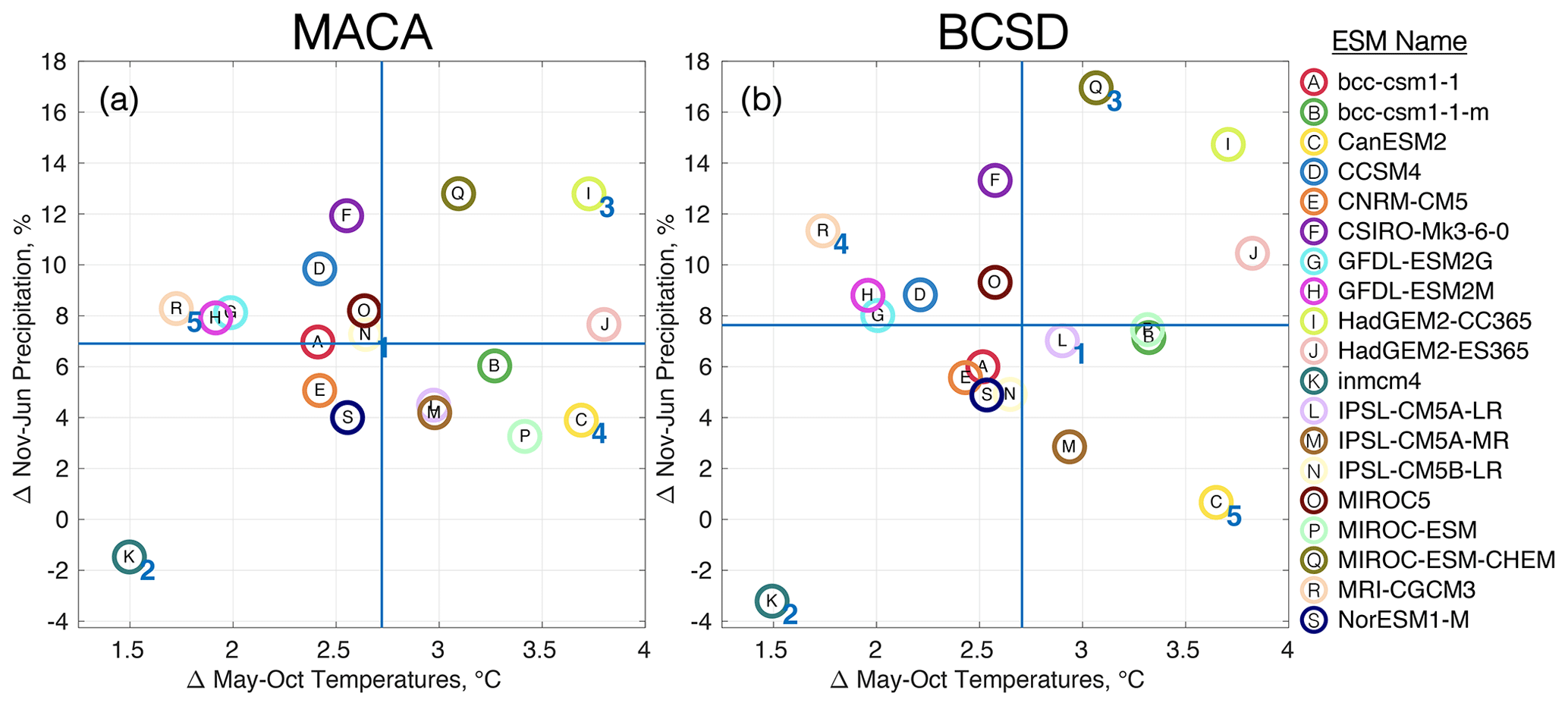
Figure 2 Relative changes in May–October temperatures and November–June precipitation over the Chesapeake Bay watershed for an ensemble of ESMs (circled letters) downscaled using (a) MACA and (b) BCSD methodologies. Horizontal and vertical blue lines correspond to the ensemble average changes in temperature and precipitation. Numbers adjacent to particular ESMs in both panels denote the order in which the first five were selected by the KKZ algorithm.

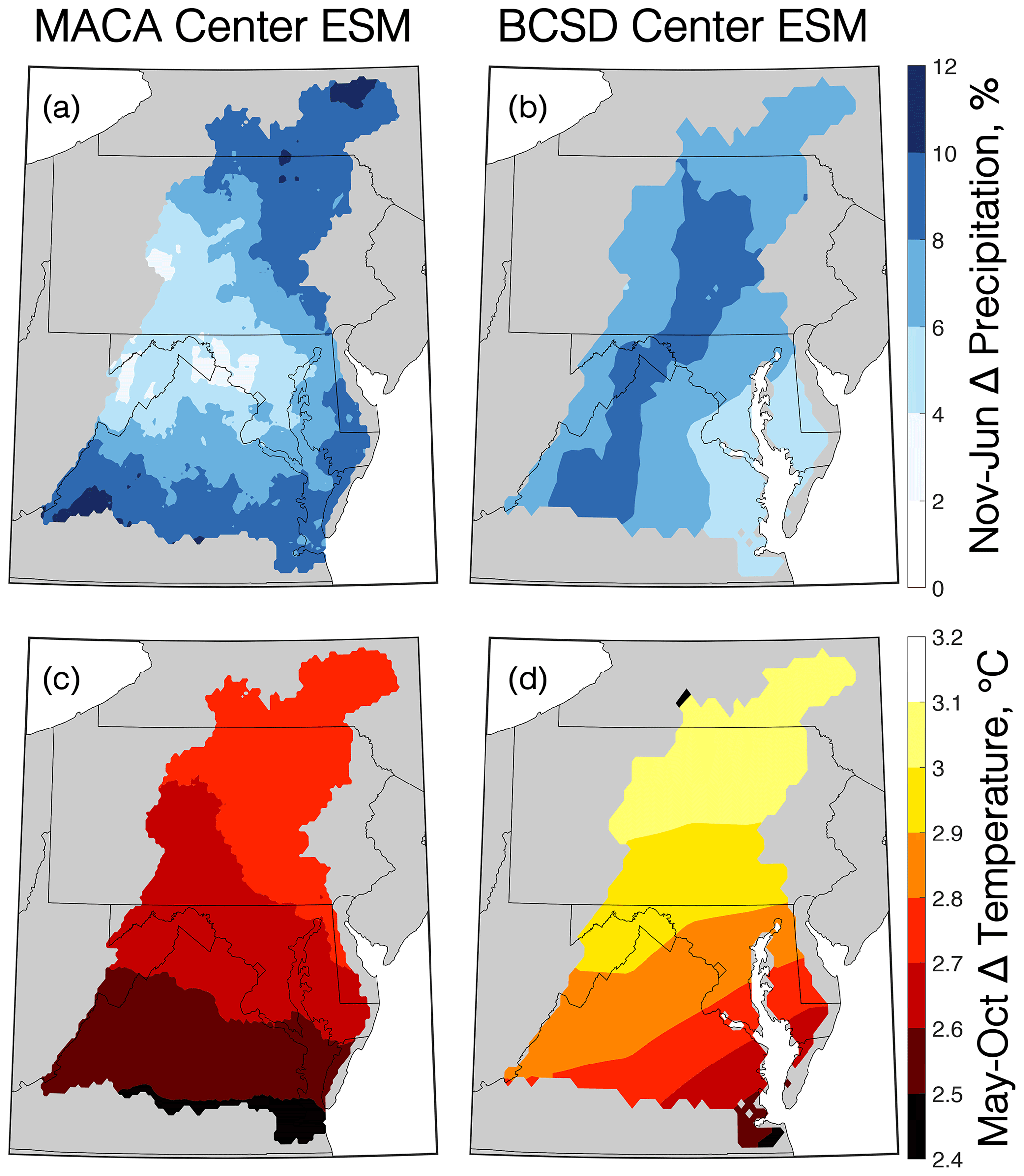
Figure 3 Changes in November to June precipitation (a, b) and May to October temperatures (c, d) for the MACA (a, c) and BCSD (b, d) center ESMs between mid-century (2046–2055) and the reference period (1991–2000). Base map layers from Pawlowicz (2020).

2.4 Experiments

Three numerical experiments (sets of simulations) were conducted to evaluate the impacts of climate scenario factors, management conditions, and the use of a subset of ESMs on future AHV projections and uncertainty (Table 1). To isolate climate impacts on AHV from the watershed alone, direct atmospheric and oceanic forcings to the bay were held to be the same as in the reference simulations (see Sect. 2.3) for all experiments. The first experiment (multi-factor) evaluates the relative change in AHV (hereafter defined as ΔAHV) between the 1991–2000 and 2046–2055 time periods due to the following factors: ESM, downscaling method, and watershed model (Table 1, Fig. 4). Atmospheric deltas from 10 downscaled ESMs (five from MACA and five from BCSD) were applied directly to the two watershed models for a total of 20 simulations. A separate Phase 6 climate reference run is used to evaluate the impacts of climate alone by holding land use and nutrient applications constant. This differs slightly from the Phase 6 reference run that simulates realistic and interannually varying nutrient inputs and terrestrial conditions and is compared against observations (Sect. 2.2). Two additional simulations were conducted with Phase 6 to account for the fact that the ESMs selected by the KKZ method were not identical for MACA and BCSD (Table 1, Fig. 2).

Figure 4 Diagram of the multi-factor experimental design, comprising a total of 20 model scenarios.

Table 1 Experiments conducted to quantify future changes in annual hypoxic volume (AHV).

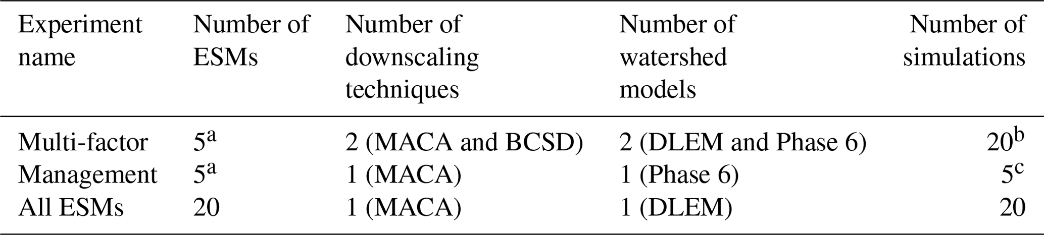
^a Corresponding to the KKZ-selected subset of the following five ESMs: center, cool/dry, hot/wet, cool/wet, and hot/dry for both MACA and BCSD downscaled model outputs. ^b Additional scenarios were simulated for the multi-factor experiment as needed (for the center and hot/wet ESMs) to accurately partition uncertainty in model outcomes. ^c An additional scenario simulated the effects of future management conditions without climate change impacts.

The second experiment (management) applied the same deltas used for Phase 6 MACA scenarios in the multi-factor experiment (thereby varying runoff and nutrient loading) but also included the effect of changing environmental management conditions (affecting nutrient inputs to and export from the terrestrial environment) for a total of five additional simulations. These management simulations assume that reduction targets for nutrient and sediment runoff are met in accordance with established management goals (USEPA, 2010). One additional scenario was conducted in which management goals were imposed and climate change was not.

The third experiment (all ESMs) applied all 20 MACA downscaled ESM deltas to the DLEM scenarios without any changes to management conditions, thereby only modifying changes in runoff and nutrient export without intentional nutrient reductions, for a total of 20 additional simulations. Comparing the results of the first (multi-factor) and third (all ESMs) experiments highlights the strengths and limitations of using a subset of ESMs.

2.5 Climate scenario analyses

To analyze climate impacts on Chesapeake Bay hypoxia, changes in O₂ and AHV were compared between the reference runs and the future simulations. Relative O₂ impacts introduced by the three climate scenario factors (ESM, downscaling method, and watershed model) were determined by applying an analysis of variance (ANOVA) approach to average ΔAHV estimates for each climate scenario. This method has been previously applied to the quantification of uncertainty sources in climate and hydrological applications (Hawkins and Sutton, 2009; Yip et al., 2011; Bosshard et al., 2013; Ohn et al., 2021). To use this method in this study, an average annual metric is first calculated for an outcome of interest (i.e., change in streamflow, nitrogen loading, or hypoxic volume) within the multi-factor experiment. Then, the relative uncertainty is determined by calculating the sum of squares due to individual effects for each experimental factor (ESM, downscaling method, or watershed model). Following Ohn et al. (2021), the cumulative uncertainty is quantified for successive uncertainties introduced by each factor and their interactions, removing the unexplained interaction term described in Bosshard et al. (2013). The two additional ESM scenarios described previously (Tables 1, S3) were used due to the inexact matches between MACA and BCSD ESMs selected by KKZ. Despite five ESMs being used in combination with only two downscaling methods and two watershed models in this analysis, the approach outlined (Bosshard et al., 2013; Ohn et al., 2021) accounts for this factor imbalance (five vs. two) by repeatedly subsampling combinations of two ESM scenarios from the five available. An example of this methodological approach is described in Appendix B.

Relative frequency histograms and cumulative distributions were used to quantify the overall likelihoods of increasing or decreasing ΔAHV across the entire range of future scenarios. Average changes in the spatial distribution of O₂ over the typical hypoxia season (May–September) were compared among all climate scenarios with no changes to management conditions. Results were considered significant if at least 80 % of the model scenarios tested agree on the direction of O₂ change in the estuary, as in Tebaldi et al. (2011).

3 Results

3.1 Model skill

3.1.1 Watershed models

Modeled streamflow, nitrate loading, and organic nitrogen loading from the three largest bay tributaries are comparable to observed monthly estimates derived from weighted statistical regressions (see Sect. 2.1). At the most downstream USGS stream gages on the Susquehanna, Potomac, and James rivers, both Phase 6 and DLEM streamflow estimates have higher skill (Nash–Sutcliffe efficiencies closer to 1.0) relative to nitrate- and organic-nitrogen-loading estimates (Table 2; Fig. S3 in the Supplement). Although the overall skill of Phase 6 and DLEM is similar, Phase 6 generally exhibits higher model skill than DLEM in estimating monthly nitrate loading, while DLEM demonstrates greater skill in simulating organic nitrogen loading.

Table 2 Nash–Sutcliffe efficiencies of the DLEM and Phase 6 watershed models at the most downstream stations of three major rivers for monthly estimates of streamflow and nutrient loading over the period 1991–2000. Nash–Sutcliffe efficiencies equal to 1 are indicative of perfect model skill, and negative values indicate that error variance exceeds the observed variance.

3.1.2 Estuarine model

The two reference simulations, forced with loadings from DLEM and Phase 6, demonstrate substantial skill in representing key main-stem estuarine biogeochemical variables, including O₂, NO₃, DON, primary production, and AHV (Table 3), throughout the bay's main stem. Overall, all modeled variables at the surface and bottom of the water column forced by both DLEM and Phase 6 lie within 1 standard deviation of observations. Modeled O₂ is slightly greater than spatio-temporally paired observations at the bottom and slightly lower than observations at the surface throughout the entire year (Table 3) and in the summer period of hypoxia (Fig. 5a–b), leading to a bias that is relatively small compared to the standard deviations of observed O₂ concentrations across the entire year (Table 3). Additionally, modeled O₂ performs similarly to or better than the results included in the multi-model comparison presented in Irby et al. (2016). Modeled average annual NO₃ and DON are also within the range of observations at both the surface and bottom (Table 3). Whole-bay net primary production agrees well with observed estimates (Harding et al., 2002) reported over a similar time period (Table 3). Finally, modeled AHV compares favorably to data-derived interpolated estimates (Table 3; Fig. 5c), with increased hypoxia in wet years compared to dry years. Average AHV estimates using Phase 6 and DLEM inputs are, respectively, 16 % and 26 % greater than interpolated observations (Table 3; Fig. 5c), and approximately half the model estimates lie within the estimated uncertainties (RMS % error) of the interpolation methodology (±13 %; Bever et al., 2018). Model estimates of AHV are generally slightly greater when ChesROMS-ECB is forced by DLEM watershed outputs as opposed to those from Phase 6 (Table 3; Fig. 5c).

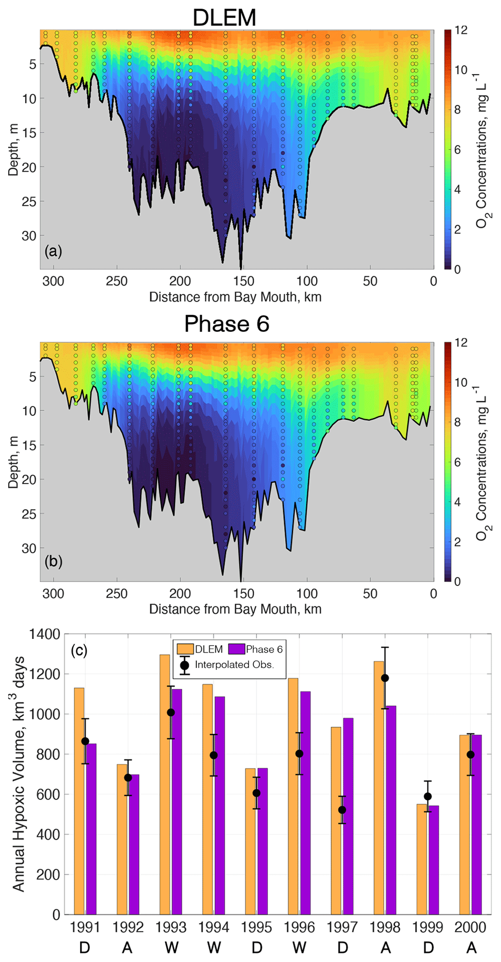
Figure 5 ChesROMS-ECB skill for average summer (June–August) O₂ profiles at main-stem monitoring locations using watershed inputs from (a) DLEM and (b) Phase 6 over the reference period 1991–2000. (c) Modeled AHV using DLEM and Phase 6 compared to interpolated observations (error bars denote RMS error) over the reference period 1991–2000. Average hydrologic conditions are noted below corresponding years and signify dry (D), average (A), or wet (W) years.

Table 3 Model skill metrics over the reference period (1991–2000).

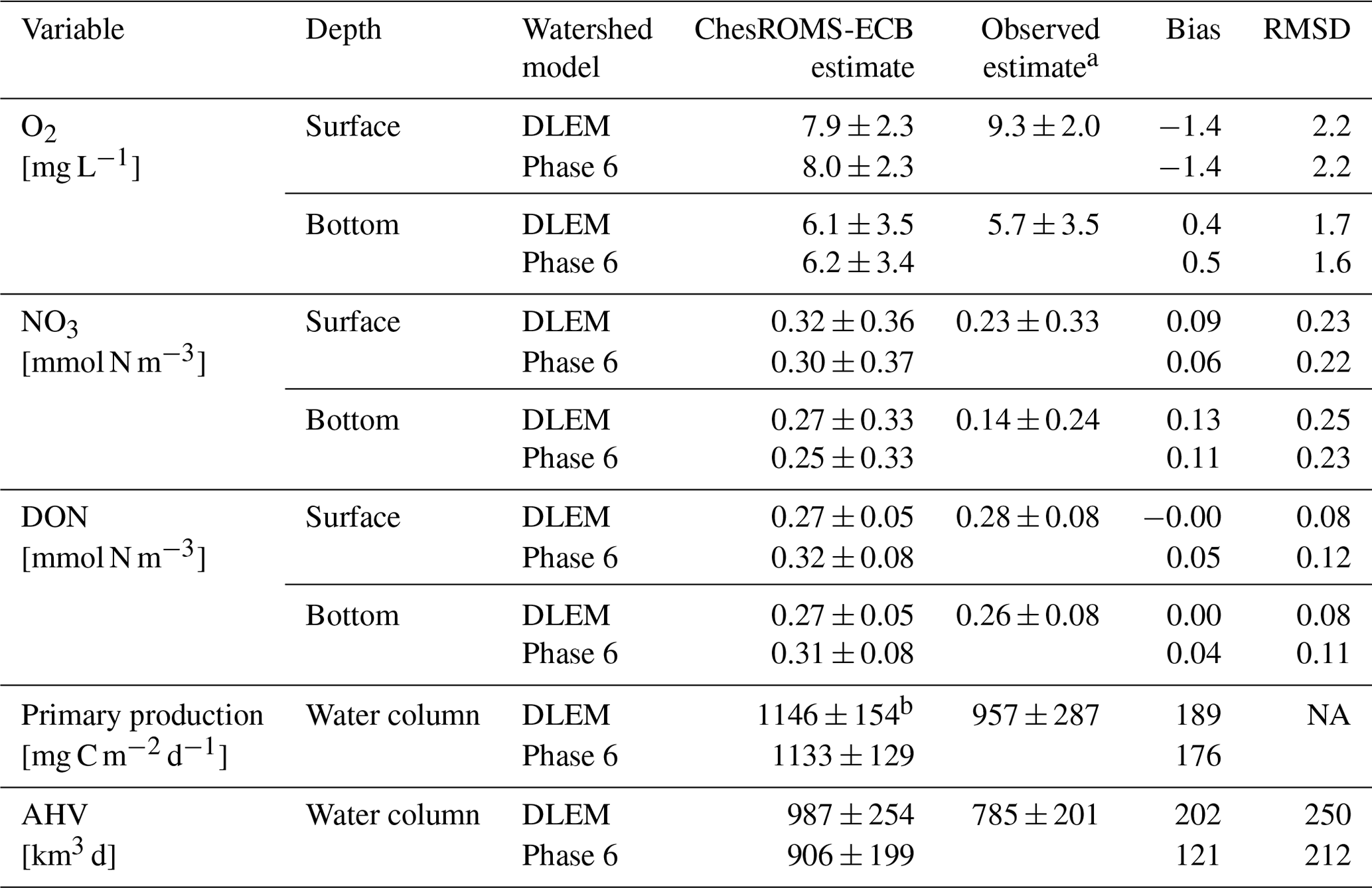
^a Observed estimates and standard deviations for O₂, NO₃, and DON are from Water Quality Monitoring Program data (Chesapeake Bay Program DataHub, 2022) at 20 main-stem stations. The observed estimate and standard error for primary production are derived from Harding et al. (2002), averaged over February–November for the years 1982–1998. The observed estimate and standard deviation for AHV is derived by applying a weighted-distance interpolation model to observed O₂ at a limited number of stations (Bever et al., 2013). ^b Modeled primary production is computed only over February–November for comparison with the observed estimate. NA: not available.

3.2 Future (mid-21st century) projections of watershed streamflow and nutrient loading

Increasing temperatures and changing precipitation throughout the bay watershed produce different streamflow responses for the two watershed models. On average, Phase 6 climate scenarios increase watershed runoff relative to the reference run by 4 %–6 %, while DLEM climate scenarios decrease average flow by 1 %–4 % (Table 4). The annual flow changes range from −12 % to +15 % among ESM scenarios, with wetter ESMs tending to increase annual watershed streamflow, while drier ESM scenarios generally decrease average watershed runoff, with a lesser impact due to atmospheric warming (Table 4; Fig. 6a). For both watershed models and downscaling methods, the cool/wet ESM produces the greatest increase in annual streamflow. Overall, the greatest variability in changes to streamflow estimates is due to the ESM, as MACA and BCSD scenarios increase or decrease annual streamflow by comparable amounts (Table 4; Fig. 6a).

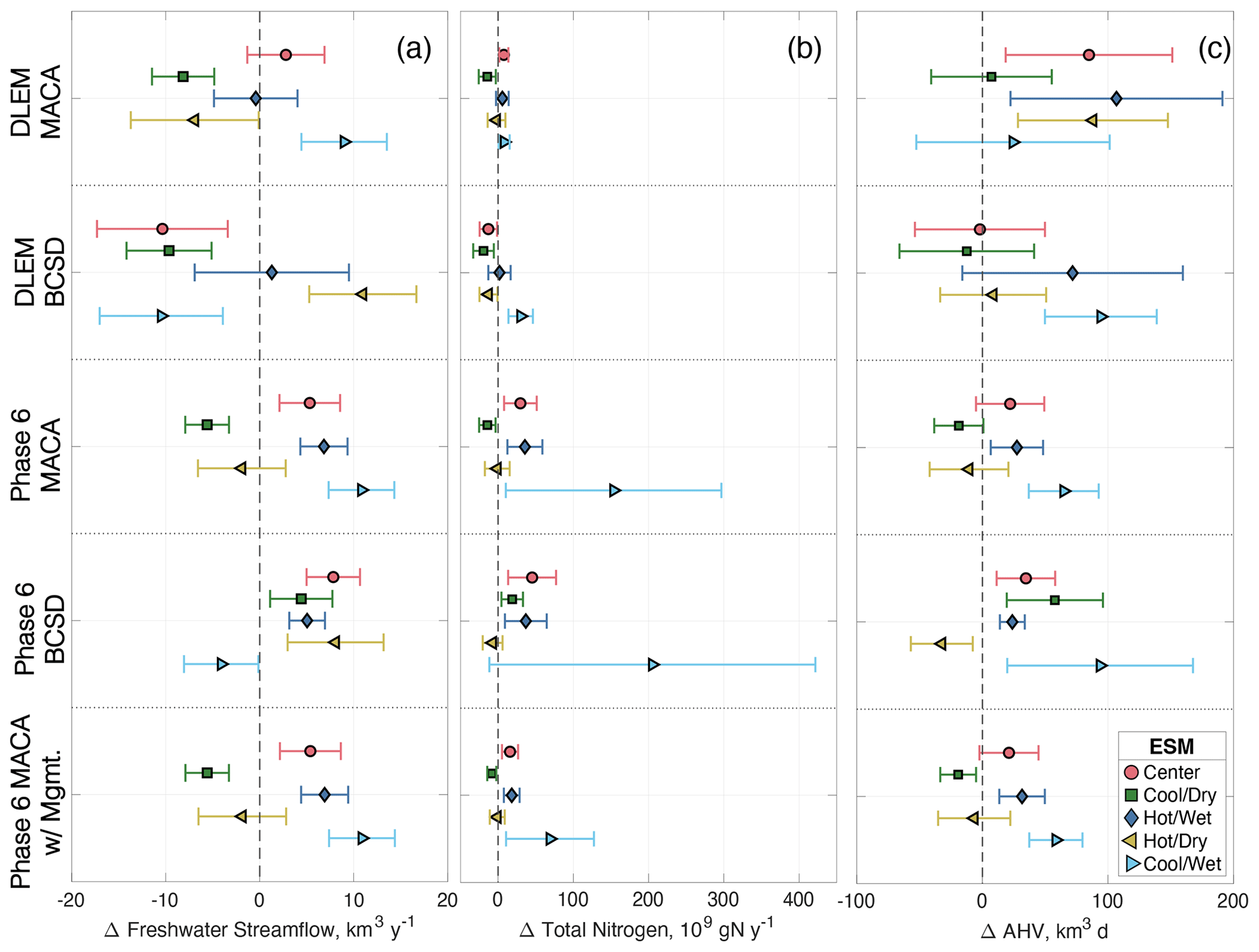
Figure 6 Mean and standard deviations of changes to freshwater streamflow (a), total nitrogen loadings (b), and annual hypoxic volume (c) for multi-factor and management experiments. Future climate changes in these outputs are shown relative to 1990s baseline conditions (dashed vertical line) without management actions (upper four rows) and with management actions (bottom row).

Table 4 Annual average and standard deviations of reference (1991–2000) and climate scenario (2046–2055) watershed loadings and estuarine hypoxia.

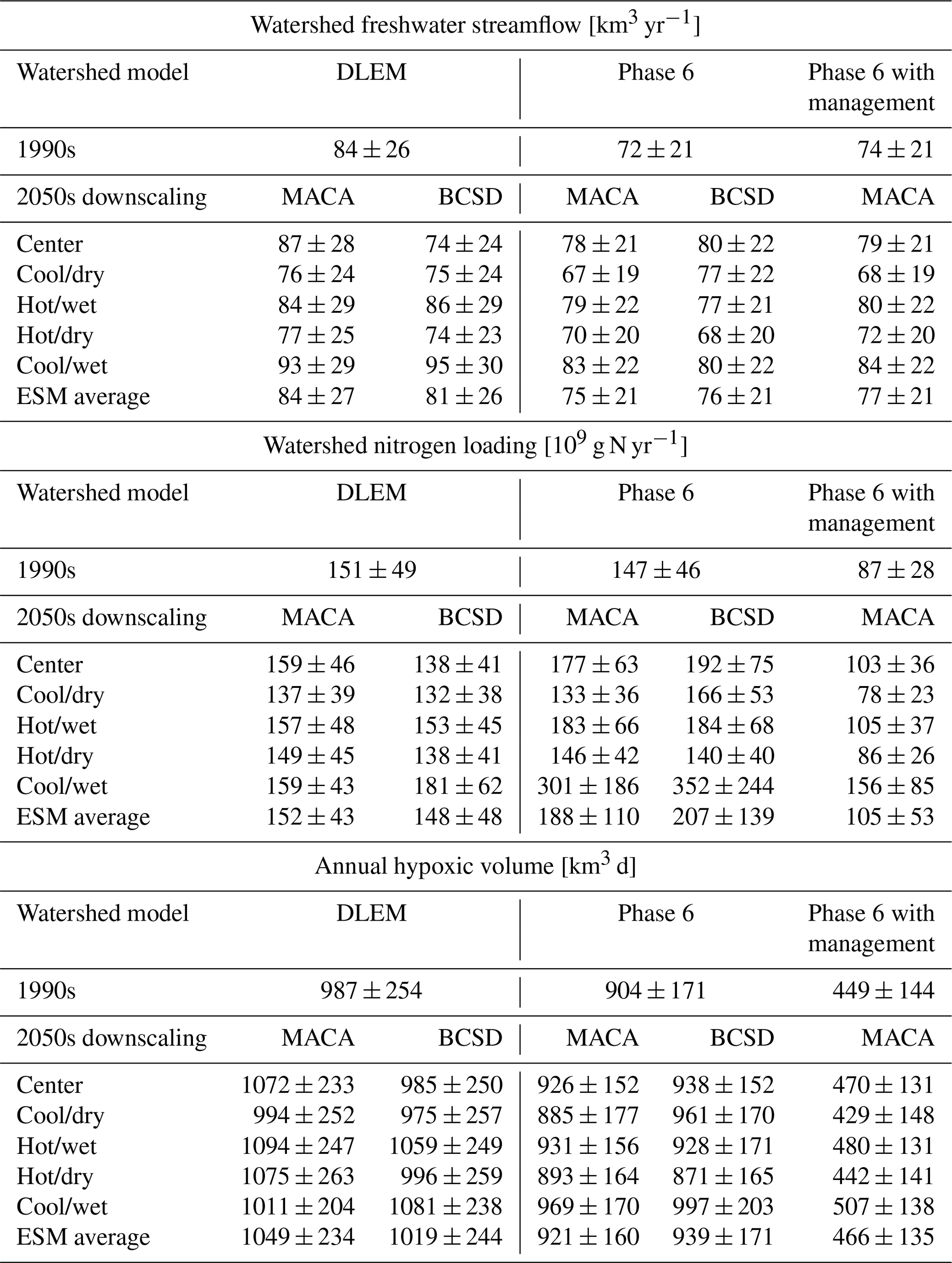
Chesapeake Bay Phase 6 watershed model climate scenarios increase average annual total nitrogen (TN) by +30 % and +45 % for MACA and BCSD, respectively, but do not substantially change DLEM TN loads (+1 % and −2 % for MACA and BCSD, respectively; Fig. 7). Greater Phase 6 TN loadings are primarily due to extreme values in the cool/wet climate scenarios and are driven by increases in refractory DON (Fig. 7a). While DLEM scenarios show increases in the percentage of inorganic nitrogen and labile organic forms of total nitrogen loads, the contribution of particulate organic nitrogen (PON) decreases, resulting in little to no increase in overall TN loading (Fig. 7a). Phase 6 produces wetter climate scenarios that increase TN loading more than drier scenarios (Table 4; Fig. 6b), with this effect being most pronounced for the cool/wet ESM. Phase 6 also produces the greatest percent changes in the southern rivers (James, York, and Rappahannock), while DLEM produces similar percent changes in all rivers (Fig. 7b). Some Phase 6 climate scenarios substantially increase the average loading change in smaller watersheds like the Rappahannock and York, which increases TN between 77 %–172 % and 32 %–430 %, respectively, and are comparable to the absolute change in Susquehanna TN loading (Fig. 7b). In contrast with the multi-factor experiment results, climate scenarios that include management actions substantially reduce TN loading (−28 %; Fig. 7, Table 4). Like other Phase 6 climate scenarios that do not account for management actions, the proportion of refractory organic nitrogen increases for the climate scenarios with management (+49 %), but in these cases, the average labile inorganic and organic nitrogen loadings also substantially decrease (−40 %).

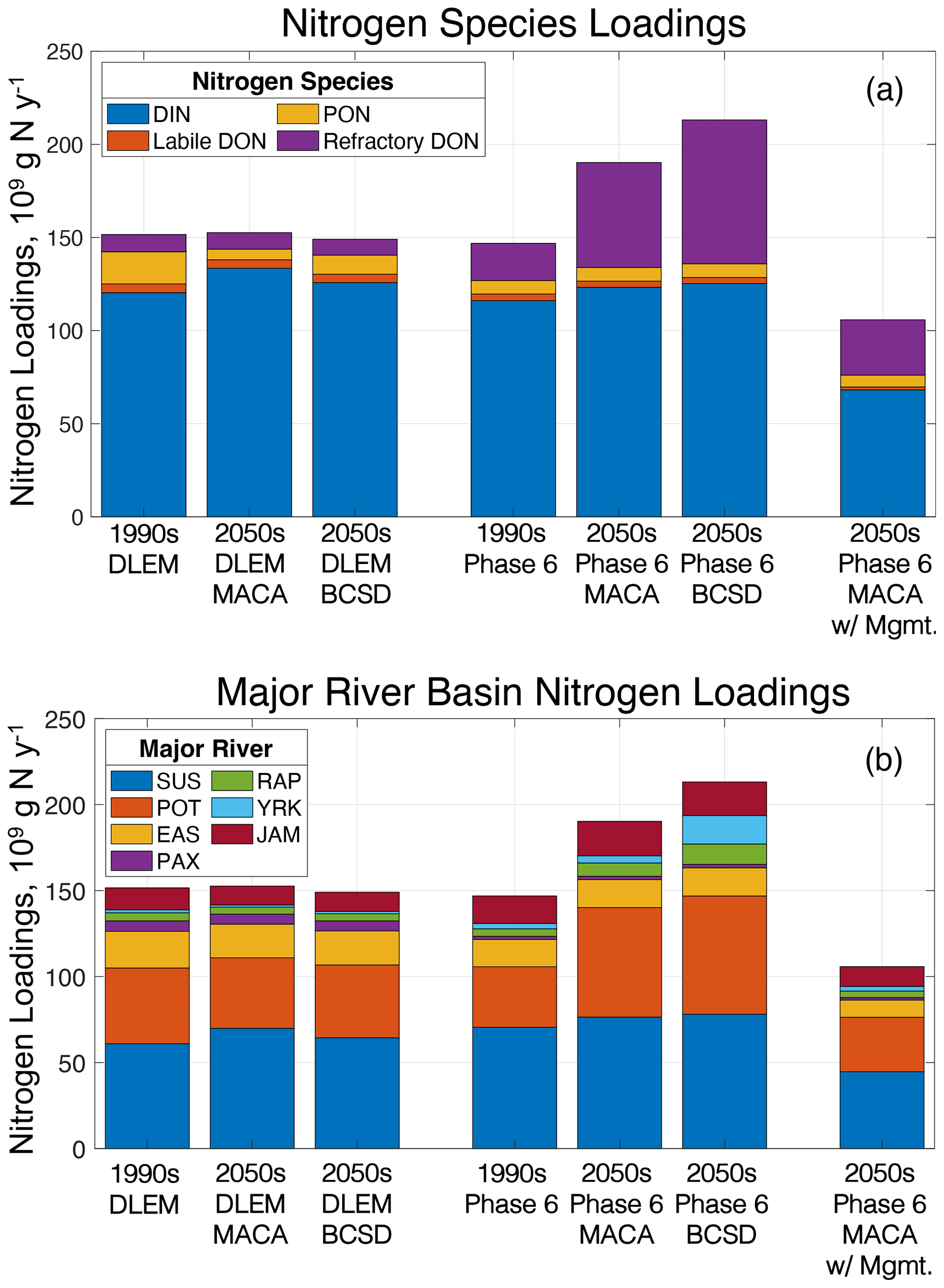
Figure 7 Average total nitrogen loadings among ESM scenarios for reference scenarios and various components of the multi-factor and management experiments. Total nitrogen loadings divided by (a) nitrogen species components, namely dissolved inorganic nitrogen (DIN), particulate organic nitrogen (PON), dissolved organic nitrogen (DON), and refractory dissolved organic nitrogen; and (b) by major river basin (SUS – Susquehanna, RAP – Rappahannock; POT – Potomac; YRK – York; EAS – eastern shore rivers, including the Elk, Chester, Choptank, and Nanticoke; JAM – James; PAX – Patuxent).

3.3 Effects of future watershed change on estuarine O₂

Climate change impacts on watershed streamflow and nitrogen loading substantially affect estuarine hypoxia, even when, as in this study, direct climate effects on the bay are not considered. On average, the multi-factor climate scenarios decrease average summer bottom O₂ in the bay's main stem while also slightly increasing O₂ at the surface in some mid-bay areas (Fig. 8). In the northern part of the main stem near the Susquehanna River outfall, model results show consistent decreases in both bottom and surface summer O₂ (Fig. 8e, f). Further down the main stem in the mid-bay, surface O₂ increases in wet years and experiences almost no change in dry years (Fig. 8b, c). In the same region, bottom O₂ declines lessen during wet years and worsen during dry years (Fig. 8e, f). Increasing O₂ levels are found in the shallow portions of the major tidal tributaries (i.e., Potomac and James) but are more pronounced in wet years than in dry years (Fig. 8b–c, e–f). Altogether, average summer surface O₂ increases by 0.02±0.03 mg L⁻¹ (average change and standard deviation), while bottom O₂ decreases by 0.03±0.06 mg L⁻¹.

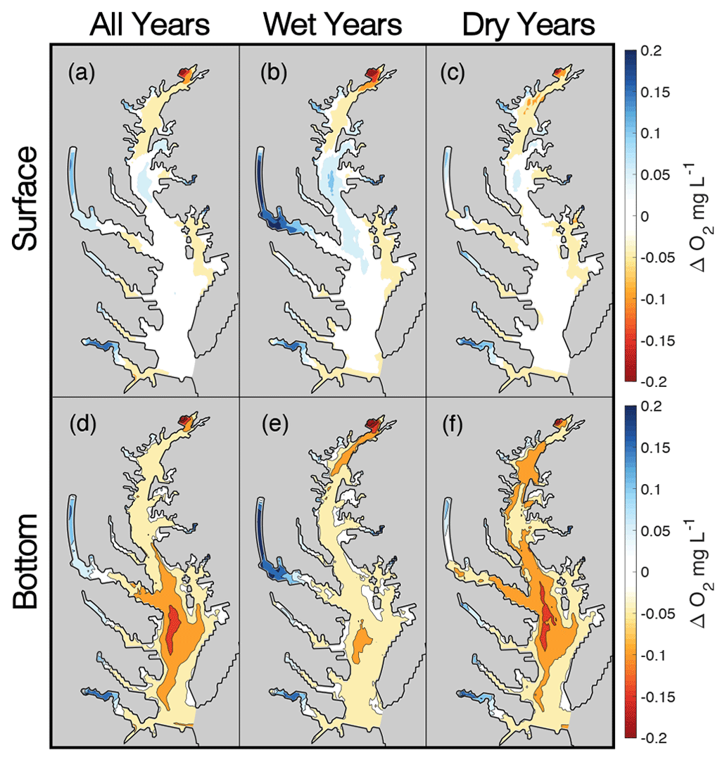
Figure 8 Average O₂ changes in multi-factor experiment scenarios at the surface (a–c) and bottom (d–f) of the water column. Columns correspond to average changes for all years (a, d) and for hydrologically wet (b, e) and dry (c, f) years.

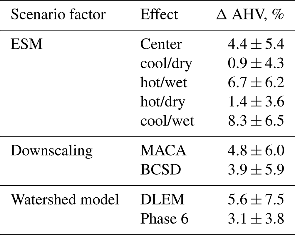
There are some clear distinctions in the overall changes to future AHV when evaluating all multi-factor experiments. Climate effects on the watershed in DLEM increase AHV more than in Phase 6 (5.6 % vs. 3.1 %, respectively), but the overall standard deviation of DLEM ΔAHV results are greater than those for Phase 6 (Table 5). Similarly, using MACA vs. BCSD results in greater changes in ΔAHV (4.8 % vs. 3.9 %); albeit, this difference due to the choice of downscaling method is less than that due to the choice of watershed model. Depending on the choice of ESM, ΔAHV ranges between +0.9 % (for the cool/dry ESM) to +8.3 % (for the cool/wet ESM), with the center ESM producing intermediate results (+4.4 %). When comparing the impact of a particular ESM, wetter models tend to produce greater ΔAHV than drier scenarios (Fig. 6c), although interannual variability is still large. When climate scenarios are downscaled using different methodologies (either MACA or BCSD), average ΔAHVs have some notable differences; e.g., applying the cool/dry model to Phase 6 produces opposite average changes to hypoxia depending on the downscaling method (Fig. 6c). Considering all possible combinations of scenarios, ESM average annual projected AHV spans a range of 921–939 km³ d for Phase 6 and 1019–1049 km³ d for DLEM, and four out of five of the climate scenarios in the multi-factor experiment project increases in average AHV (Table 4).

Table 5 Average ±standard error in ΔAHV (%) holding scenario effects (ESM, downscaling method, and watershed model) constant.

When the full distribution of multi-factor scenarios is evaluated, the average and standard deviation of these annual ΔAHV results are estimated to be 37±64 km³ d (4.4 ± 7.4 %; Fig. 9). Wetter ESMs (blues in Fig. 9a) are more likely to increase hypoxia compared to drier ESMs, despite differences in downscaling method or watershed model. The likelihoods of the cool/dry or hot/dry ESMs increasing hypoxia are only 58 % or 50 %, respectively, but these chances are greater than 80 % for the center, hot/wet, and cool/wet ESMs (Fig. 9a). Altogether, the multi-factor experiment results in 72 % of the runs increasing AHV when considering climate change impacts on terrestrial runoff (Fig. 9b). Note, however, that this cannot technically be considered to be a statistical probability, as the KKZ selection process used to generate our sample of climate scenarios is neither random nor independent.

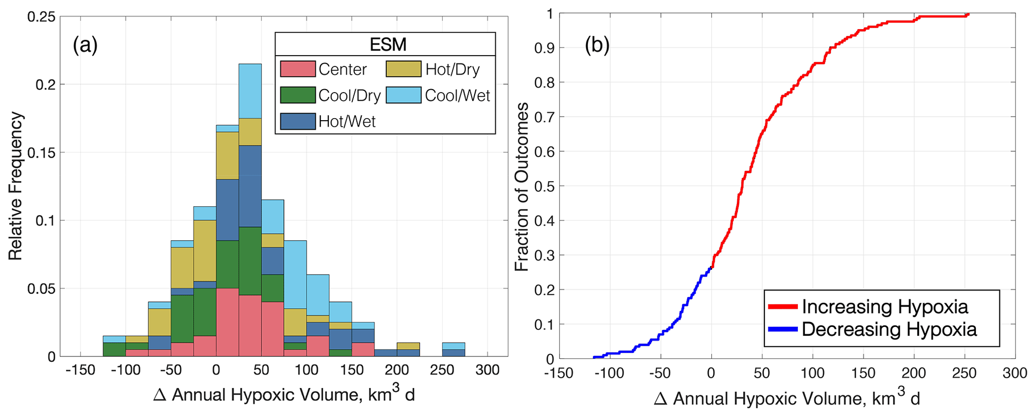
Figure 9 Summary of multi-factor experiment results for changes to annual hypoxic volume, expressed as a histogram of relative frequencies (a) and an empirical cumulative distribution (b).

The all-ESMs experiment produces similar results to those obtained when only a subset of five ESMs is used. Specifically, ΔAHV increases by 6.3 ± 3.5 % using only 5 KKZ-selected ESMs and by 9.6 ± 1.7 % when using all 20 ESMs (Fig. 10a, b; model IDs are further defined in Table S3 in the Supplement). The use of 5 KKZ-selected ESMs covers approximately 69 % of the total range of all 20 ESMs (Fig. 10c). Despite more than 15 000 options to choose from when selecting 5 out of 20 ESMs, the subset selected in this work demonstrates an improved ability to outperform a random selection of 5 ESMs (Fig. 10c) and generates a useful range of hypoxia projections.

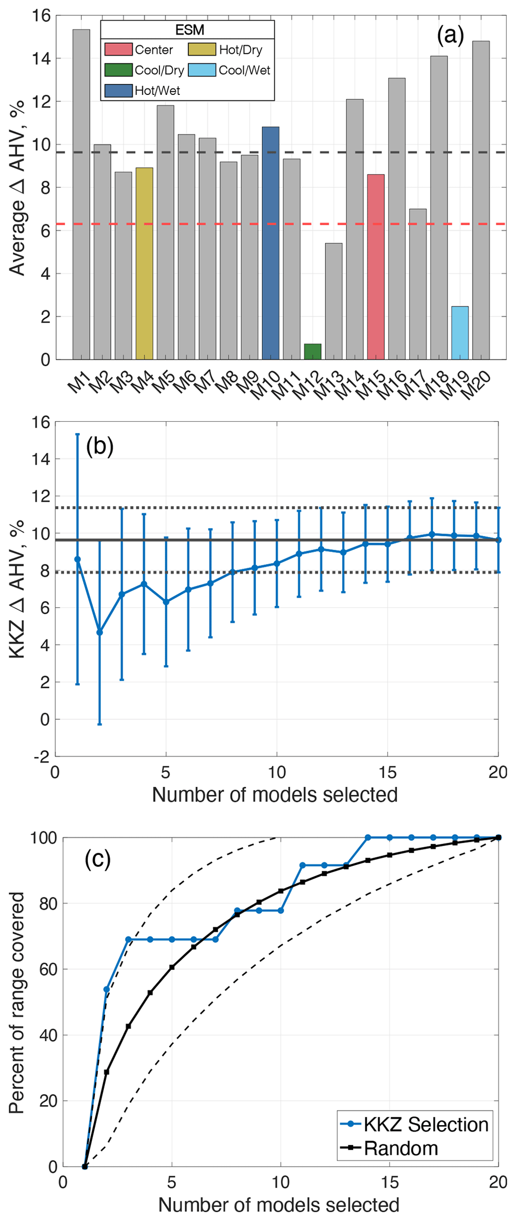
Figure 10 (a) Change in annual hypoxic volume (ΔAHV) for the all-ESMs experiment. The dashed red line denotes the multi-model average of five KKZ-selected ESMs; the dashed black line denotes the full 20-model average. (b) ΔAHV and standard errors as estimated by increasing the number of KKZ-selected ESMs. The black lines correspond to the 20-model average (solid) and associated standard errors (dotted) from the all-ESMs experiment. (c) Percent of ΔAHV range covered by sequentially increasing the number of KKZ-selected ESMs. The black lines correspond to the range (solid) and associated standard error (dashed) of estimates chosen by randomly selecting ESMs.

The results of the management experiment demonstrate the substantial impact of future nutrient reductions on hypoxia, decreasing average ΔAHV by 50 ± 7 % relative to the 1990s (ΔAHV = $-\mathrm{438}\pm \mathrm{47}$ km³ d; Table 4; Fig. 11). Because there is a linear relationship between ΔAHV computed with Phase 6 MACA scenarios including management actions (ΔAHV_mgmt) and those without (ΔAHV = 0.56 ⋅ ΔAHV_mgmt − 262; R² = 0.59; Fig. S4), ΔAHV_mgmt can be estimated for any scenario by applying this linear model to the non-management-scenario distribution. In effect, this linear relationship demonstrates a similar magnitude of relative nutrient export to and consequent hypoxia within the estuary. The result is a decrease of approximately 417 ± 67 km³ d among all scenarios, within the range of the management scenario subset obtained here by applying only MACA downscaled ESMs to Phase 6. As expected, hypoxia increases in the management experiment when climate impacts are also included relative to the reference management scenario, specifically by 17.1±34.8 km³ d or 3.8 ± 7.8 % (Table 4; Fig. 6c).

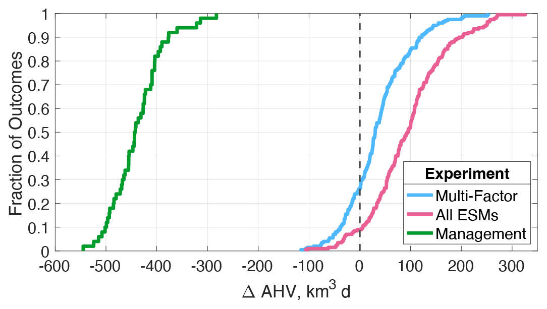
Figure 11 Summary of all experiment results for change in annual hypoxic volume (ΔAHV), expressed as a cumulative distribution function. The vertical dashed black line corresponds to no change in AHV.

3.4 Contributions to climate scenario uncertainty

Applying an ANOVA approach (Ohn et al., 2021) to watershed streamflow, nutrient loadings, and ΔAHV within the multi-factor experiment reveals that the relative uncertainties introduced by the choice of ESM, downscaling method, and watershed model vary substantially (Fig. 12). The choice of ESM is the dominant factor affecting changes to watershed streamflow and nutrient loadings (Fig. 12a–c) and comprises 59 %–74 % of the total uncertainty. The choice of watershed model is the next largest source of uncertainty, making up 17 %–34 % of the total variance in watershed changes, while the downscaling method only contributes 3 %–14 %. Uncertainty in projected organic nitrogen loadings is particularly affected by the choice of watershed model, overwhelming the variability introduced by downscaling method and strongly affecting estimates of total nitrogen change. Unlike changes to watershed flow and loadings, the uncertainty of projected changes to hypoxia is much more evenly distributed among the three scenario factors, specifically 40 %, 25 %, and 35 % for the ESM, downscaling method, and watershed model, respectively (Fig. 12d).

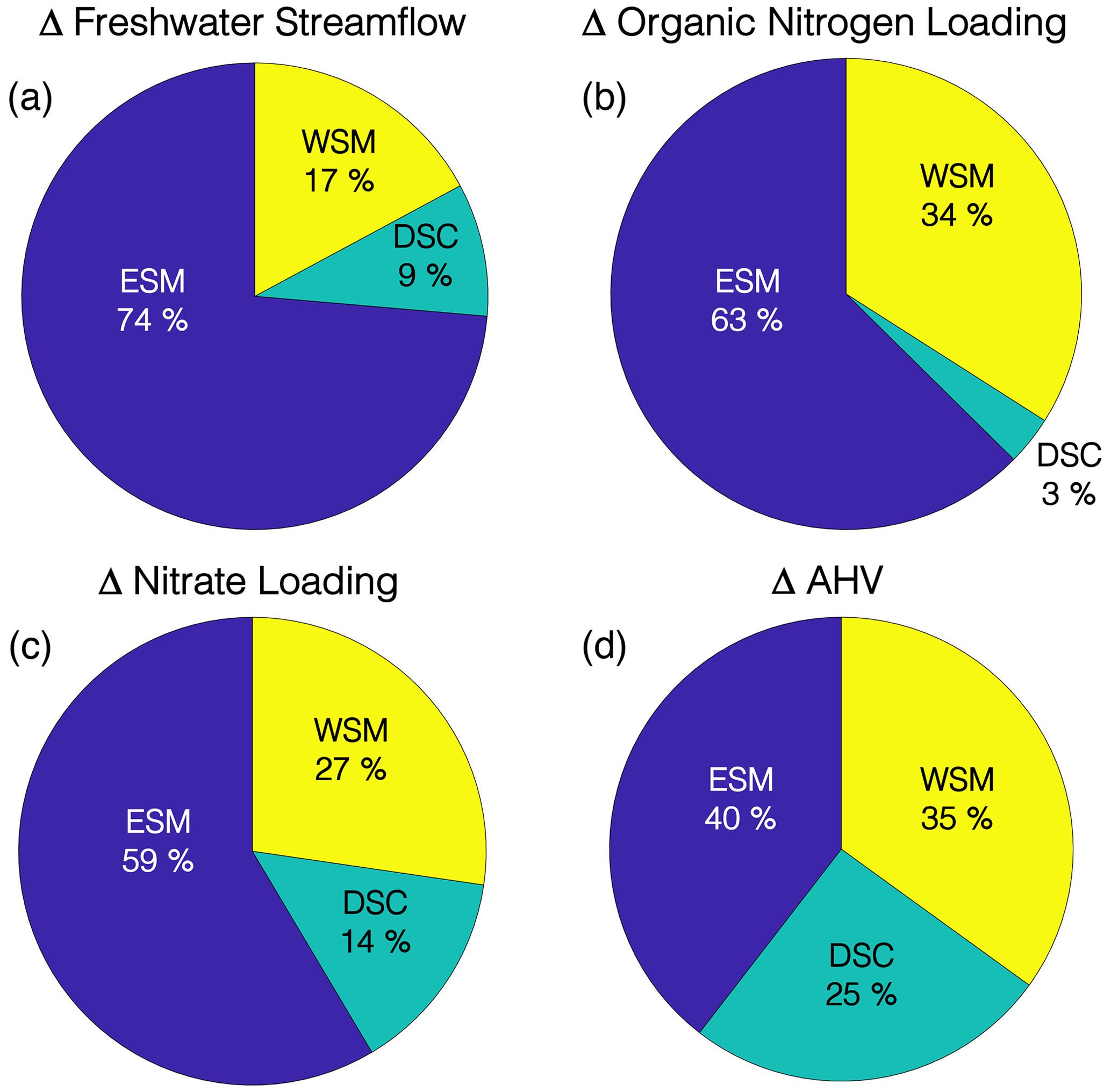
Figure 12 Percent contribution to uncertainty from the Earth system model (ESM), downscaling methodology (DSC), and watershed model (WSM) for estimates of (a) freshwater streamflow, (b) organic nitrogen loading, (c) nitrate loading, and (d) change in annual hypoxic volume (ΔAHV).

4 Discussion

4.1 Uncertainty in climate scenario projections

Projected changes in watershed streamflow and nutrient delivery to Chesapeake Bay produce modest increases in estuarine hypoxia with medium confidence (Mastrandrea et al., 2010). Hypoxic volume has a high degree of interannual variability, and future hypoxia estimates are highly sensitive to the choice of ESM, downscaling method, and watershed model (Fig. 6c). Although certain factors (particularly ESM and greenhouse gas emission scenarios; Meier et al., 2021) have previously been extensively evaluated in coastal systems with regards to future hypoxia, the results presented here also demonstrate the importance of terrestrial forcings on estuarine oxygen levels.

In this study, future changes in watershed streamflow, nitrogen loadings, and estuarine hypoxia are found to be highly dependent on the selection of a specific ESM (Fig. 12), with this factor comprising the majority of the total uncertainty in watershed runoff and the greatest fraction of total uncertainty for O₂ levels. When only the effect of ESM choice is considered (and downscaling and hydrological model options are not; Fig. 10), the average projected change in AHV using only three ESMs (often chosen to represent cool, median, and hot scenarios) has a greater standard error than the selection of five ESMs using KKZ in this study. Directly comparing results from the experiment that compared five ESMs, two downscaling methods, and two watershed models (multi-factor) versus that which only considered the impact of multiple ESMs (all ESMs) shows a substantial overlap in the range of projected ΔAHV. In addition, multiple ESMs downscaled with a single methodology and applied to one hydrological model produced meaningfully different estimates of ΔAHV than a more balanced approach (Fig. 11).

Inter-model variability among ESMs appears to contribute most substantially to differences in bay watershed inputs, but the choice of downscaling methodology can also affect these projections. The BCSD (Wood et al., 2004) and MACA (Abatzoglou and Brown, 2012) downscaling methodologies used here employ different approaches to reduce historical ESM biases, impacting the variability of spatio-temporal watershed hydrologic and water quality responses. The ability to statistically downscale ESMs accurately depends on the spatially coarser ESM's ability to simulate synoptic-scale (∼ 1000 km) patterns and may still underestimate the distributional tails of changes to temperature and precipitation. This increases the importance of properly selecting a subset of ESMs (Abatzoglou and Brown, 2012).

Watershed model variability is caused by differences in the representation of processes that affect streamflow, those controlling the fate and transport of nutrients from land and in rivers, and lag times of groundwater transport. The two watershed models used here project substantially different results in watershed streamflow and nitrogen delivery, even when the same changes to meteorological forcings are applied (Fig. 6). DLEM projects no change or decreases in streamflow for nearly all scenarios as opposed to greater average increases in streamflow for Phase 6 scenarios (Fig. 6a), likely driven by differences in the representation of evapotranspiration. Explicit soil biogeochemical processes within DLEM increase nitrification rates in warmer-climate scenarios, producing higher nitrate loadings than Phase 6 despite comparable streamflow changes (Fig. 6b). The greater total nitrogen loadings produced by Phase 6 are largely a consequence of its parameterizations for erosion and refractory nitrogen bound to sediment. Increases in bioavailable nitrate loadings, unlike refractory organic nitrogen that comprises the majority of DON loadings, produce greater levels of primary production and remineralization within the estuary. This largely explains the discrepancy between watershed model hypoxia estimates (Table 5).

Our findings demonstrate the importance of considering differences among these three factors (ESM, downscaling, and watershed model) that may contribute to a wider range of target water quality variables and living-resource responses in coastal marine ecosystems like Chesapeake Bay that are highly influenced by watershed processes. Hydrological model assumptions can have potentially significant impacts on estuarine hypoxia. For example, the relatively high organic nitrogen loadings in Phase 6 compared to DLEM's comparatively modest exports under the same future scenarios result in different levels of annual hypoxia. While dramatic increases in organic nitrogen loadings within bay tributaries are mostly limited to cool/wet Phase 6 scenarios, there is precedent for catastrophic erosion within the bay watershed driven by extreme precipitation events (Springer et al., 2001). The relative uncertainty introduced by individual factors is also not necessarily equivalent for streamflow, nitrogen loadings, and AHV (Fig. 12). The complex connections between terrestrial runoff and biogeochemical changes in the marine environment may expand further when higher-order trophic-level species are considered and even more so when direct atmospheric impacts on the bay are also included. It is unlikely that general conclusions regarding the relative impacts of different factors can be drawn for a marine ecosystem when only uncertainties in watershed streamflow and nutrient loadings are considered. Had our results only accounted for the impacts of these factors on watershed changes and not estuarine oxygen levels, the role of downscaling could be incorrectly assumed to contribute negligible variability to hypoxic volume (Fig. 12). It is the complex interactions of nitrogen species transformations within this estuarine model that are responsible for this somewhat unexpectedly large contribution of downscaling-method uncertainty that is less prominent in watershed changes.

Despite the relatively small magnitude of Chesapeake Bay watershed climate impacts on estuarine hypoxia compared to previous evaluations of other climate impacts, like atmospheric warming over the bay (Irby et al., 2018; Ni et al., 2019; Tian et al., 2021), the relative contributions of ESM and downscaling effects to the total uncertainty are large and are also likely to expand the range of outcomes for other climate sensitivity studies in this region. This suggests that, when attempting to determine a likely range of ecosystem outcomes, selecting additional downscaling techniques and hydrological model responses should be considered in addition to the more common practice of only selecting multiple ESMs.

4.2 Watershed climate scenario impacts on riverine export and hypoxia

The climate scenario projections evaluated in this study are in near-complete agreement that the Chesapeake Bay watershed will be warmer and will experience greater levels of precipitation by the mid-century, yet these results are not as straightforward to interpret, as they relate to changes in streamflow, nutrient loads, and estuarine hypoxia. Climate impacts on extreme river flows are currently evident at global scales (Gudmundsson et al., 2021), and projected increases in precipitation that could shape such events are aligned with estimates for this region derived from observational (Yang et al., 2021) and modeling (Huang et al., 2021) studies, as well as for other regions at similar latitudes (Bevacqua et al., 2021; Madakumbura et al., 2021). However, differences exist in the spatial distribution and timing of these precipitation increases, as well as in the temperature-affected rates of evapotranspiration. As a result, these estimates produce varied projections for future freshwater streamflow. These complex interactions make it difficult to directly predict future streamflow from projected precipitation changes and even more difficult to relate these to changes in nutrient loading. For example, in this study, half of the climate scenarios produce increasing streamflow on an annual basis, yet more than 75 % of these scenarios increase total nitrogen loading. Differences in the representation of soil and riverine nitrogen processes between watershed models also result in inconsistent simulated responses of nitrogen export to similar precipitation rates. Disparate export of nitrogen species (i.e., nitrate and organic nitrogen) between watershed models also directly affects future nutrient load projections. These hydrological model differences are evidenced by DLEM's higher NO₃ outputs that offset lower organic nitrogen loadings (Fig. 7a).

Table 6 A summary comparison of simulated mid-21st century climate change impacts on Chesapeake Bay hypoxia relative to observed conditions.

AAV – annual anoxic volume; AHV – annual hypoxic volume. ^a AAV defined as O₂ < 1 mg L⁻¹ in Wang et al. (2017) and O₂ < 0.2 mg L⁻¹ for all others. ^b Applied downscaled ESMs in projecting changes to Chesapeake Bay hypoxia. ^c No 2050 estimate provided; results based on 2025 projected changes.

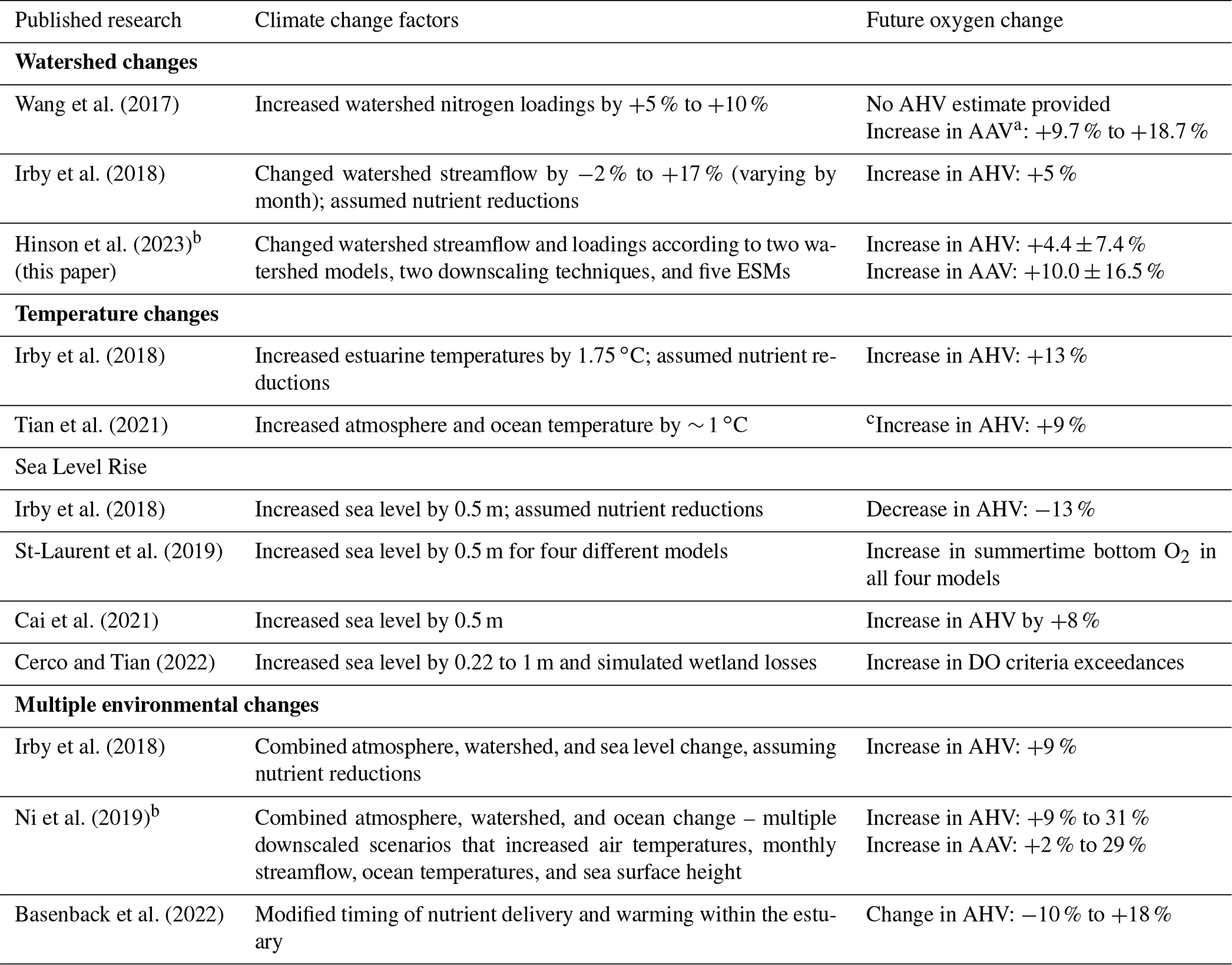
Our analysis quantifies changes in hypoxia due to mid-century climate change impacts on the watershed and provides an estimate of the relative uncertainty in these estimates. Our experimental findings suggest that, in the absence of management actions, mid-century climate impacts on the Chesapeake Bay watershed will increase hypoxia, specifically annual hypoxic volume (AHV), by an average of 4 ± 7 %. This estimate is in good agreement with prior studies that examined the impacts of watershed actions alone. Irby et al. (2018) applied a sensitivity approach and projected increases in AHV of 5 %, while Wang et al. (2017) showed increases in annual anoxic volume of 9.7 %, nearly equivalent to the increase of 10 ± 16.5 % found here (Table 6). Results from this study also project that changes to bay O₂ levels will vary spatially. Average bottom main-stem O₂ levels from May–September are expected to decrease most in the southern half of the bay (south of 38.5^∘ N), particularly in climatologically dry years (Fig. 8).

Importantly, the projected changes presented here only account for the effects of climate change on watershed response in isolation and do not include the additional direct impacts of the atmosphere and ocean. These additional changes have been estimated in other previous studies of 21st century impacts relative to observed conditions (Table 6). While numerous differing metrics have been reported for many of these studies, including shifting dissolved-oxygen concentrations and water quality regulatory criteria, this work can be compared against previous results by examining changes to annual hypoxic and anoxic volumes. The majority of these studies (Table 6) apply idealized changes to climate forcings and generally project increases in hypoxic conditions. Increases in mid-21st century annual hypoxic volume due to watershed forcings (+5 % and +4.4 ± 7.4 %) are smaller than the average impacts of increasing temperatures alone (+13 %), while the results of changing sea level are more mixed (Table 6). However, the variability in hypoxia due to watershed changes is likely greatest among these factors and may substantially modify the negative effects of warming on dissolved-oxygen concentrations. Our results and their uncertainties generally encompass the range of future hypoxia estimates found in previous research that has studied multiple climate impacts in isolation and in various combinations. Future work that accounts for the sources of uncertainty explored here by applying realistic climate change projections while also standardizing a metric for model results, like annual hypoxic volume, will help to narrow and better quantify definitive trends due to multiple factors that influence bay dissolved oxygen.

Our findings are focused on Chesapeake Bay hypoxia, but some lessons can also be drawn from other coastal ecosystems where changes in watershed streamflow and nutrient loadings are also projected. In the Baltic Sea, Meier et al. (2011b) reported that hypoxia was very likely to increase regardless of ESM or climate scenario, assuming targeted reductions in accordance with the Baltic Sea Action Plan (decrease of nitrogen loads by 23 ± 5 %) were not met. Extensive studies of projected oxygen change in the Baltic Sea have repeatedly demonstrated that climate impacts are likely to increase hypoxic area (BACC II Author Team, 2015, and references therein), but more recent reports (Saraiva et al., 2019a; Wåhlström et al., 2020; Meier et al., 2021, 2022) have reaffirmed that nutrient reductions in accordance with the Baltic Sea Plan are also highly likely to mitigate a substantial amount of those hypoxia increases. Repeated investigations into the impact of increased streamflow and higher temperatures in the Gulf of Mexico demonstrate a likely expansion of hypoxic area (Justić et al., 1996; Lehrter et al., 2017; Laurent et al., 2018) and that additional nutrient reductions would be required to mitigate these impacts (Justić et al., 2003). Finally, Whitney and Vlahos (2021) demonstrated a considerable erosion in oxygen gains in Long Island Sound due to nutrient reductions in the presence of climate effects, reducing projected mid-century improvements by 14 %, similar to the 9 % increase in hypoxic volume reported by Irby et al. (2018) for O₂ levels <2 mg L⁻¹. Although these studies include direct climate change impacts on coastal water bodies, most support the findings here, demonstrating that increases in streamflow and associated nutrient loadings are likely to increase Chesapeake Bay hypoxia. Overall, climate impacts on land have the potential to profoundly modify biogeochemical interactions in the coastal zone and to limit the efficacy of nutrient reductions.

4.3 Hypoxia lessened by impacts of management actions

Projections of changes to watershed streamflow and nutrient delivery can better inform regional environmental managers tasked with managing interactions among nutrient reduction strategies, climate change, and coastal hypoxia (Hood et al., 2021; BACC II Author Team, 2015; Fennel and Laurent, 2018). The Chesapeake Bay results provided in this analysis demonstrate that the management actions mandated to improve water quality (USEPA, 2010) will decrease hypoxia by roughly 50 %, approximately an order of magnitude more than projected increases due only to watershed climate change (Fig. 11). Therefore, nutrient reduction strategies are very likely to remain effective at reducing watershed nutrient loading and its contribution to eutrophication and hypoxia over a range of possible ESM scenarios (Mastrandrea et al., 2010). Should all management actions be implemented as outlined in the USEPA's Total Maximum Daily Load (USEPA, 2010), it is very likely that future climate impacts on bay watershed runoff will worsen bay hypoxia by a far smaller amount relative to 1990s reference conditions. These findings are consistent with those of Irby et al. (2018), who also examined the impacts of watershed climate on Chesapeake Bay hypoxia for the mid-21st century. When evaluating the effects of watershed climate impacts and management actions together, Irby et al. (2018) estimated an average AHV increase of 12.8 km³ d, which is well within the range of 17.1 ± 34.8 km³ d reported here (Table 6). Additionally, the combined impact of all climate stressors reported by Irby et al. (2018), i.e., atmosphere, ocean, and watershed, increased average AHV by 24.5 km³ d, which is also within the range of the results reported here. Because climate change impacts are likely to increase total nitrogen loads, implementing nutrient reductions that do not account for the detrimental effects of climate change will reduce the likelihood of attaining water quality targets. Further quantifying a range of future estimates of watershed streamflow and nitrogen loading using regional models is critical to understanding the possibilities and limitations of mitigating negative climate impacts via nutrient reductions.

Recent findings support the hypothesis that nutrient reductions will improve water quality despite projected climate impacts in both freshwater systems (Wade et al., 2022) and other coastal marine systems (Whitney and Vlahos, 2021; Saraiva et al., 2019a; Bartosova et al., 2019; Wåhlström et al., 2020; Pihlainen et al., 2020; Meier et al., 2021; Große et al., 2020; Jarvis et al., 2022). In Chesapeake Bay, reduced nutrient loading (Zhang et al., 2018; Murphy et al., 2022) has already helped mitigate growing climate change pressures (Frankel et al., 2022) despite rapidly increasing bay temperatures over the past 30 years (Hinson et al., 2021). Like these prior studies, our findings confirm that management actions will likely produce even greater benefits to O₂ in coastal zones strongly affected by terrestrial runoff. While direct effects (e.g., air temperature) are expected to increase hypoxia more than watershed changes in Chesapeake Bay (Irby et al., 2018; Ni et al., 2019), the comparatively greater impacts of management actions reported here are also likely to substantially reduce the overall risk from a multitude of co-occurring climatic stressors.

4.4 Study limitations and future research directions

Despite the plainly evident finding of nutrient reduction strategies improving water quality and counteracting negative climate change watershed impacts, a number of important caveats should temper this conclusion. First, the subset of scenarios that include management actions is limited to a set of five ESMs statistically downscaled with a single methodology and applied to one watershed model. As demonstrated in this work, this assumption may oversimplify the complex relationship between climate forcings and watershed model simulations, especially given that DLEM scenarios produce more change in nitrate and consequently more hypoxia than Phase 6 scenarios. Management actions implemented in Phase 6 nutrient reduction scenarios represent a multitude of possible methods to reduce point and nonpoint source pollution that are assumed to be fully implemented with a high operational efficacy by the mid-century, but the true performance of the best management practices operating under future hydroclimatic stressors remains largely unresolved (Hanson et al., 2022). Additionally, the importance of legacy nitrogen inputs to the bay may grow over time (Ator and Denver, 2015; Chang et al., 2021) and can only be properly accounted for via a long-term transient simulation that accounts for changing groundwater conditions.

A key strength of the delta method applied here is its ability to remove the influence of interannual variability, which is known to strongly influence hypoxia in Chesapeake Bay (Bever et al., 2013). However, the delta method is unable to account for the impacts of unanticipated extreme events or changing patterns of precipitation intensity, duration, and frequency that produce dramatic responses in sediment washoff, scour, and consequent watershed organic nitrogen export. Air temperature and precipitation were the only watershed model input variables adjusted in this analysis, allowing for a more equivalent comparison between downscaling approaches. Future representations of watershed change may also better account for changes in runoff through the inclusion of factors like ESM-estimated relative humidity that can help avoid possible unreasonable amplification of potential evapotranspiration that would decrease tributary streamflow (Milly and Dunne, 2011) and associated nutrient loads.

Although main-stem bay oxygen levels are the focus of this study, watershed impacts are also likely to influence water quality in smaller-scale tributaries. Differences in Chesapeake Bay temperatures introduced by the ESM and downscaling method have also been investigated by Muhling et al. (2018) and contribute to biogeochemical variability via the direct impacts of atmospheric temperature on bay warming. Incorporating different facets of these relative uncertainties into projections of coastal change has also been demonstrated to affect ecological outcomes like those surrounding fisheries (Reum et al., 2020; Bossier et al., 2021). Thus, the impacts of these uncertainties are also very likely to affect socio-economic systems tied to coastal resources. The analytical method applied here is well established within climatic and terrestrial settings, so the relative dearth of coastal applications (excluding Meier et al., 2021) may be more related to a consequence of computational demand or a greater focus on uncertain parameterizations of marine biogeochemical processes (Jarvis et al., 2022) that also play a large role in potential future hypoxia outcomes.

5 Conclusions

Coastal ecosystems like Chesapeake Bay that are currently and will likely continue to be negatively affected by climate impacts exhibit complex responses in future scenarios, demonstrating our lack of complete system understanding. While this research reaffirms the importance of management actions in reducing levels of hypoxia, it also highlights the fact that uncertainties in climate-impacted watershed conditions will affect estimates of Chesapeake Bay O₂ levels. Additional study of uncertainty interactions within a full climate scenario (that includes the impacts of changing atmospheric and oceanic conditions) will help better quantify a range of hypoxia projections among other environmental conditions within Chesapeake Bay. These results underscore the need for additional rigorous analyses of model parameterizations and their contributions to model scenario uncertainty to help identify biogeochemical processes that are most sensitive to climate change impacts and warrant further investigation. The development of more rapid techniques to evaluate a broader range of future water quality and ecological outcomes, and an inspection of their underlying assumptions, can help provide a better mechanistic understanding of complex reactions to multiple climate stressors. Like ongoing efforts to reduce greenhouse gas emissions and to lessen the impacts of future climate change globally, continuing efforts to reduce eutrophication in coastal waters could help improve ecosystem resilience and the benefits derived by communities dependent on their function. Nutrient reduction plans are likely to become even more essential to managers tasked with preserving the health and functioning of rapidly evolving coastal environments and unfamiliar future conditions.

Appendix A

Original partitioning of organic nitrogen pools from the DLEM and Phase 6 watershed models was based on fixed fractions previously described in Frankel et al. (2022). There, 80 % of the refractory organic nitrogen (rorN) loadings from Phase 6 were allocated to the small detritus nitrogen (SDeN) pool, and the remainder were applied to the refractory dissolved organic nitrogen (rDON) pool in ChesROMS-ECB. More realistic changes to this partitioning of watershed rorN loadings were implemented, which decreased the lability of organic nitrogen loads overall. A specified threshold of rorN loadings was set at the 90th percentile of reference Phase 6 watershed inputs to the estuarine model, and thresholds were also set for individual river levels of streamflow at the 50th and 90th percentiles of Phase 6 reference simulations. Below the 50th percentile of streamflow levels, 80 % of the rorN inputs below the specified rorN threshold were allocated to ChesROMS-ECB's SDeN pool, and the remainder were assigned to the rDON pool. Between the 50th and 90th percentiles of streamflow events, 50 % of the rorN load below the specified rorN threshold was apportioned to ChesROMS-ECB's SDeN and rDON pools. At the uppermost levels of streamflow (greater than the 90th percentile), 5 % of rorN was allocated to SDeN, and 95 % was given to rDON within ChesROMS-ECB. For any partitioning of an organic nitrogen load, regardless of the level of streamflow, rorN loading above this cutoff was allocated to ChesROMS-ECB's rDON pool. The rorN load below this threshold was allocated according to the fractionations described above. Changes to Phase 6 watershed loadings were mapped to equivalent DLEM watershed input variables following the methodology of Frankel et al. (2022).

Abbreviation	Definition
AHV	Annual hypoxic volume
BCSD	Bias correction and spatial disaggregation
CBP	Chesapeake Bay Program
ChesROMS-ECB	Chesapeake Regional Ocean Modeling System – Estuarine Carbon and Biogeochemistry
CMIP	Coupled Model Intercomparison Project
DIN	Dissolved inorganic nitrogen
DLEM	Dynamic Land Ecosystem Model
DON	Dissolved organic nitrogen
DSC	Downscaling methodology
ESM	Earth system model
KKZ	Katsavounidis–Kuo–Zhang (Katsavounidis et al., 1994)
MACA	Multivariate Adapted Constructed Analogs
Phase 6	Phase 6 Watershed Model
RCP	Representative Concentration Pathway
WSM	Watershed model

Appendix B

An example calculation of the methodology used to calculate the uncertainty for a single component of the total uncertainty is provided below. Average annual changes in hypoxic volume (km³ d) are shown for the multi-factor experiment. Values of hypoxic volume are rounded to the 10th decimal place in Tables B1–B3, but the rounding is not carried through all calculations.

For the first calculation, a subset of two ESMs is selected so that the number of values is balanced among ESMs, downscaling methods, and watershed models (Table B2). This process will be repeated for each possible combination of ESMs, of which there are 10 in total $\mathit{\left\{}\right(\mathrm{1},\mathrm{2}),(\mathrm{1},\mathrm{3}),(\mathrm{1},\mathrm{4}),\mathrm{\dots },(\mathrm{4},\mathrm{5}\left)\mathit{\right\}}$.

For simplicity, Table B2 can be rearranged to that shown in Table B3. Additionally, the formats of Table B3 and the following equations largely mirror the format of Ohn et al. (2021).

Table B1 Average change in annual hypoxic volume (units of km³ d) for the multi-factor experiment.

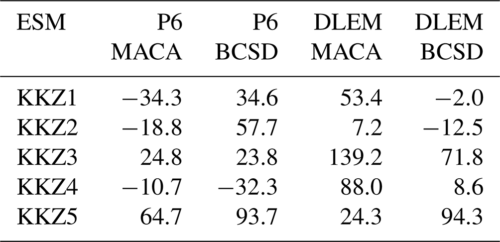
Table B2 Average changes in annual hypoxic volume (units of km³ d) for a subset of the multi-factor experiment, selected to be balanced with the two choices of downscaling method and watershed model.

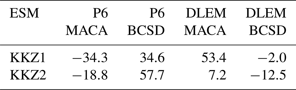
Table B3 Factorial representation of changes in annual hypoxic volume shown in Table B2. The Earth system model, downscaling method, and watershed model respectively correspond to stages 1, 2, and 3.

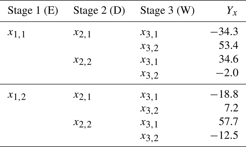
First, the total variance of this subset ($U_{\mathit{\{}\mathrm{1},\mathrm{2},\mathrm{3}\mathit{\}}}^{\mathrm{cumul}}$) is calculated, with the subscripts of each individual factor (ESM – 1, downscaling method – ,2, watershed Model – 3) denoted in brackets and N defined as the total number of possible outcomes (Y_x in Table B3).

$$U_{\mathit{\{}\mathrm{1},\mathrm{2},\mathrm{3}\mathit{\}}}^{\mathrm{cumul}}={\displaystyle \frac{\mathrm{1}}{N}}\sum _i^N{\left(X_i-\stackrel{\mathrm{‾}}{X}\right)}^{\mathrm{2}}=\mathrm{1025.1}$$

Following this, the cumulative uncertainty due to the choice of downscaling method and watershed model ($U_{\mathit{\{}\mathrm{1},\mathrm{2}\mathit{\}}}^{\mathrm{cumul}}$) is calculated by selecting all Y_x values from Table B3, where the first two stages vary (Y_{1,2}) but the third stage does not (either (x_3,1) or (x_3,2)).

$$\begin{array}{c}{\displaystyle }{Y}_{\mathit{\{}\mathrm{1},\mathrm{2}\mathit{\}}}\left(x_{\mathrm{3},\mathrm{1}}\right)=\mathit{\{}-\mathrm{34.3},\mathrm{34.6},-\mathrm{18.8},\mathrm{57.7}\mathit{\}}\\ {\displaystyle }{Y}_{\mathit{\{}\mathrm{1},\mathrm{2}\mathit{\}}}\left(x_{\mathrm{3},\mathrm{2}}\right)=\mathit{\{}\mathrm{53.4},-\mathrm{2.0},\mathrm{7.2},-\mathrm{12.5}\mathit{\}}\\ {\displaystyle }\begin{array}{rl}{U}_{\left\{\mathrm{1},\mathrm{2}\right\}}^{\mathrm{cumul}}& ={\displaystyle \frac{\mathrm{1}}{\mathrm{2}}}\left(U_{\left\{\mathrm{1},\mathrm{2}\right\}}^{\mathrm{cumul}}\left(x_{\mathrm{3},\mathrm{1}}\right)+U_{\left\{\mathrm{1},\mathrm{2}\right\}}^{\mathrm{cumul}}\left(x_{\mathrm{3},\mathrm{1}}\right)\right)\\ & ={\displaystyle \frac{\mathrm{1}}{\mathrm{2}}}\left(\mathrm{1417.0}+\mathrm{631.7}\right)=\mathrm{1024.3}\end{array}\end{array}$$

Similar variance calculations are completed for the uncertainty of the first stage alone ($U_{\mathit{\left\{}\mathrm{1}\mathit{\right\}}}^{\mathrm{cumul}}$), where the choice of ESM is the only constant.

$$\begin{array}{c}{\displaystyle }{Y}_{\mathit{\left\{}\mathrm{1}\mathit{\right\}}}\left(x_{\mathrm{2},\mathrm{1}},x_{\mathrm{3},\mathrm{1}}\right)=\mathit{\{}-\mathrm{34.3},-\mathrm{18.8}\mathit{\}}\\ {\displaystyle }{Y}_{\mathit{\left\{}\mathrm{1}\mathit{\right\}}}\left(x_{\mathrm{2},\mathrm{1}},x_{\mathrm{3},\mathrm{2}}\right)=\mathit{\{}\mathrm{53.4},\mathrm{7.2}\mathit{\}}\\ {\displaystyle }{Y}_{\mathit{\left\{}\mathrm{1}\mathit{\right\}}}\left(x_{\mathrm{2},\mathrm{2}},x_{\mathrm{3},\mathrm{1}}\right)=\mathit{\{}\mathrm{34.6},\mathrm{57.7}\mathit{\}}\\ {\displaystyle }{Y}_{\mathit{\left\{}\mathrm{1}\mathit{\right\}}}\left(x_{\mathrm{2},\mathrm{2}},x_{\mathrm{3},\mathrm{2}}\right)=\mathit{\{}-\mathrm{2.0},-\mathrm{12.5}\mathit{\}}\end{array}$$

Combining these values to calculate the uncertainty of the first stage alone (ESM) yields the following equation, where i and j denote the factor choices from stages 2 and 3 in Table B3:

$$\begin{array}{rl}{U}_{\mathit{\left\{}\mathrm{1}\mathit{\right\}}}^{\mathrm{cumul}}& ={\displaystyle \frac{\mathrm{1}}{\mathrm{4}}}\sum _{i=\mathrm{1}}^{\mathrm{2}}\sum _{j=\mathrm{1}}^{\mathrm{2}}\left(Y_{\mathit{\left\{}\mathrm{1}\mathit{\right\}}}\left(x_{\mathrm{2},i},x_{\mathrm{3},j}\right)\right)\\ & ={\displaystyle \frac{\mathrm{1}}{\mathrm{4}}}\left(\mathrm{60.1}+\mathrm{533.6}+\mathrm{133.4}+\mathrm{52.6}\right)\approx \mathrm{188.2}.\end{array}$$

Applying similar calculations produces the following values, which are necessary to compute the total uncertainty for all stages:

$$\begin{array}{c}{\displaystyle }{U}_{\mathit{\{}\mathrm{1},\mathrm{2},\mathrm{3}\mathit{\}}}^{\mathrm{cumul}}=\mathrm{1025.1},\\ {\displaystyle }{U}_{\mathit{\{}\mathrm{1},\mathrm{2}\mathit{\}}}^{\mathrm{cumul}}=\mathrm{1024.3},\\ {\displaystyle }{U}_{\mathit{\{}\mathrm{2},\mathrm{3}\mathit{\}}}^{\mathrm{cumul}}=\mathrm{1019.9},\\ {\displaystyle }{U}_{\mathit{\{}\mathrm{1},\mathrm{3}\mathit{\}}}^{\mathrm{cumul}}=\mathrm{947}.,\mathrm{7}\\ {\displaystyle }{U}_{\mathit{\left\{}\mathrm{1}\mathit{\right\}}}^{\mathrm{cumul}}=\mathrm{188.2},\\ {\displaystyle }{U}_{\mathit{\left\{}\mathrm{2}\mathit{\right\}}}^{\mathrm{cumul}}=\mathrm{877.7},\\ {\displaystyle }{U}_{\mathit{\left\{}\mathrm{3}\mathit{\right\}}}^{\mathrm{cumul}}=\mathrm{913.4}.\end{array}$$

Next, the uncertainty of the first stage is calculated by subtracting the uncertainties from other stages as follows:

$$\begin{array}{c}{\displaystyle }{U}_{\left\{\mathrm{1},\mathrm{2},\mathrm{3}\right\},\mathrm{1}}^{\mathrm{cumul}}=U_{\mathit{\{}\mathrm{1},\mathrm{2},\mathrm{3}\mathit{\}}}^{\mathrm{cumul}}-U_{\left\{\mathrm{2},\mathrm{3}\right\}}^{\mathrm{cumul}}=\mathrm{5.2},\\ {\displaystyle }{U}_{\left\{\mathrm{1},\mathrm{2}\right\},\mathrm{1}}^{\mathrm{cumul}}=U_{\mathit{\{}\mathrm{1},\mathrm{2}\mathit{\}}}^{\mathrm{cumul}}-U_{\left\{\mathrm{2}\right\}}^{\mathrm{cumul}}=\mathrm{146.6},\\ {\displaystyle }{U}_{\left\{\mathrm{1},\mathrm{3}\right\},\mathrm{1}}^{\mathrm{cumul}}=U_{\mathit{\{}\mathrm{1},\mathrm{3}\mathit{\}}}^{\mathrm{cumul}}-U_{\left\{\mathrm{3}\right\}}^{\mathrm{cumul}}=\mathrm{34.3},\\ {\displaystyle }{U}_{\left\{\mathrm{1}\right\},\mathrm{1}}^{\mathrm{cumul}}=\mathrm{188.2}.\end{array}$$

The combined value of the cumulative uncertainty for the first stage (ESM) can now be calculated as follows:

$$\begin{array}{rl}& {\displaystyle \frac{\mathrm{1}}{\mathrm{3}}}\left(U_{\left\{\mathrm{1},\mathrm{2},\mathrm{3}\right\},\mathrm{1}}^{\mathrm{cumul}}+{\displaystyle \frac{\mathrm{1}}{\mathrm{2}}}{U}_{\left\{\mathrm{1},\mathrm{2}\right\},\mathrm{1}}^{\mathrm{cumul}}+{\displaystyle \frac{\mathrm{1}}{\mathrm{2}}}{U}_{\left\{\mathrm{1},\mathrm{3}\right\},\mathrm{1}}^{\mathrm{cumul}}+U_{\left\{\mathrm{1}\right\},\mathrm{1}}^{\mathrm{cumul}}\right)\\ & ={\displaystyle \frac{\mathrm{1}}{\mathrm{3}}}\left(\mathrm{5.1}+\mathrm{73.3}+\mathrm{17.2}+\mathrm{188.2}\right)=\mathrm{94.6}.\end{array}$$

Applying the same computational steps results in cumulative uncertainties for stages 2 (downscaling method) and 3 (watershed model) of 475.5 and 480.5, respectively. These values correspond to relative uncertainties for the ESM, downscaling method, and watershed model of 9 %, 45 %, and 46 %, respectively. This procedure is then repeated for all other combinations of two ESMs $\mathit{\left\{}\right(\mathrm{1},\mathrm{3}),(\mathrm{1},\mathrm{4}),(\mathrm{1},\mathrm{5}),\mathrm{\dots },(\mathrm{4},\mathrm{5}\left)\mathit{\right\}}$ , after which the percentage values are averaged to produce the estimates reported in our results.