the Creative Commons Attribution 4.0 License.
the Creative Commons Attribution 4.0 License.
 | 06 Jun 2023
Snow–vegetation–atmosphere interactions in alpine tundra
Kristoffer Aalstad
Yeliz A. Yilmaz
Astrid Vatne
Andrea L. Popp
Peter Horvath
Anders Bryn
Ane Victoria Vollsnes
Sebastian Westermann
Terje Koren Berntsen
Frode Stordal
Lena Merete Tallaksen
The interannual variability of snow cover in alpine areas is increasing, which may affect the tightly coupled cycles of carbon and water through snow–vegetation–atmosphere interactions across a range of spatio-temporal scales. To explore the role of snow cover for the land–atmosphere exchange of CO2 and water vapor in alpine tundra ecosystems, we combined 3 years (2019–2021) of continuous eddy covariance flux measurements of the net ecosystem exchange of CO2 (NEE) and evapotranspiration (ET) from the Finse site in alpine Norway (1210 m a.s.l.) with a ground-based ecosystem-type classification and satellite imagery from Sentinel-2, Landsat 8, and MODIS. While the snow conditions in 2019 and 2021 can be described as site typical, 2020 features an extreme snow accumulation associated with a strong negative phase of the Scandinavian pattern of the synoptic atmospheric circulation during spring. This extreme snow accumulation caused a 1-month delay in melt-out date, which falls in the 92nd percentile in the distribution of yearly melt-out dates in the period 2001–2021. The melt-out dates follow a consistent fine-scale spatial relationship with ecosystem types across years. Mountain and lichen heathlands melt out more heterogeneously than fens and flood plains, while late snowbeds melt out up to 1 month later than the other ecosystem types. While the summertime average normalized difference vegetation index (NDVI) was reduced considerably during the extreme-snow year 2020, it reached the same maximum as in the other years for all but one of the ecosystem types (late snowbeds), indicating that the delayed onset of vegetation growth is compensated to the same maximum productivity. Eddy covariance estimates of NEE and ET are gap-filled separately for two wind sectors using a random forest regression model to account for complex and nonlinear ecohydrological interactions. While the two wind sectors differ markedly in vegetation composition and flux magnitudes, their flux response is controlled by the same drivers as estimated by the predictor importance of the random forest model, as well as by the high correlation of flux magnitudes (correlation coefficient r=0.92 for NEE and r=0.89 for ET) between both areas. The 1-month delay of the start of the snow-free season in 2020 reduced the total annual ET by 50 % compared to 2019 and 2021 and reduced the growing-season carbon assimilation to turn the ecosystem from a moderate annual carbon sink (−31 to −6 gC m−2 yr−1) to a source (34 to 20 gC m−2 yr−1). These results underpin the strong dependence of ecosystem structure and functioning on snow dynamics, whose anomalies can result in important ecological extreme events for alpine ecosystems.
- Article
(5379 KB) - Full-text XML
-
Supplement
(1429 KB) - BibTeX
- EndNote


At northern latitudes, the alpine tundra shares many similarities with the arctic tundra regarding its appearance, dynamics, and role in the Earth system. These ecosystems typically feature low vegetation, a shallow root zone with acidic soils, and a complex pattern of inter-dependent plant, fungal, and microbial communities that emerge across a large range of spatial scales (Walker et al., 2001). The vegetation is primarily limited by the supply of energy and nutrients, which is to a large degree governed by the spatio-temporal variability of the snow cover. In alpine tundra, the surface energy balance, soil temperatures, and nutrient availability are all directly affected by the presence of snow (Rixen et al., 2022). The snowpack moreover offers plants protection against frost damage, dehydration, and mechanical damage from wind-blown snow particles in wintertime (Mott et al., 2018). This protection comes at the price of longer-lasting snow cover limiting the growing-season length for plants (Vestergren, 1902), which is especially pronounced in topographic depressions where wind-blown snow accumulates. The vegetation structure in these characteristic snowbed–ridge ecosystems will in turn influence the wind-blown snow transport and thus modify the spatial variability of the snow distribution. These complex and consistent snow–vegetation interactions give rise to repeating patterns in snow distributions (Sturm and Wagner, 2010) and are thus a key structuring process for alpine tundra environments and an important control on land–atmosphere interactions (Odland and Munkejord, 2008).
Community ecologists have long recognized that plant associations form and thrive in specific ranges of environmental conditions (Gleason, 1926; Whittaker, 1956). However, snow–vegetation interactions and the related responses to snow cover changes in high-latitude and high-altitude ecosystems can be highly context dependent (Niittynen et al., 2018, 2020). Wipf et al. (2009) and Frei and Henry (2022) analyzed plant phenology, growth, and reproduction in alpine and arctic shrubs, respectively, and found that reductions in snow cover duration are beneficial for some but not all tundra species. Niittynen et al. (2018), on the other hand, found a tipping point at a 20 %–30 % decrease in snow cover duration, at which accelerated species loss reduces the biodiversity in arctic–alpine areas. Scharnagl et al. (2019) documented the expansion of shrubs in alpine ecosystems over a 40-year period but argue that plant community composition remained mostly intact, demonstrating a surprising resilience of alpine tundra plant communities to ongoing global climate change. Similarly, Roos et al. (2022) show that experimental warming with International Tundra Experiment (ITEX) chambers over a 30-year period in alpine Norway only had a modest effect on the community composition, while nutrient additions caused strong responses in vegetation dynamics.
There are a number of indicators for an ecosystem's interaction with the atmosphere that – while related – highlight different aspects of this coupling. The normalized difference vegetation index (NDVI), for example, has been used to document widespread greening of mountain slopes (Jia et al., 2003). Such changes can, in turn, have profound impacts on the ecosystem's carbon and water balances through increased land–atmosphere exchange of CO2 and water vapor, i.e., the net ecosystem exchange of CO2 (NEE) and evapotranspiration (ET). The link between the carbon and water cycles in terrestrial ecosystems can be assessed through the ratio of NEE and ET, known as the ecosystem water-use efficiency (as opposed to leaf-level water-use efficiency derived from photosynthesis and transpiration), which provides another key indicator for ecosystem functioning under changing environmental conditions (Niu et al., 2011; Schlesinger, 2020). If an ecosystem has been subject to biochemical or biophysical shifts due to extreme conditions, one may expect to see this reflected in the ecosystem's water-use efficiency. In arctic tundra, NEE estimates show that longer growing seasons due to earlier snow melt-out may not necessarily lead to stronger carbon assimilation because tundra ecosystems may not be able to continue to take up CO2 late in the growing seasons (Groendahl et al., 2007; Zona et al., 2022). Evapotranspiration in high-latitude ecosystems is normally limited by net surface radiation and is thus typically small compared to total annual precipitation (Liljedahl et al., 2011), while lower-latitude alpine grasslands can feature ET losses of more than 50 % of the total annual precipitation (Carrillo-Rojas et al., 2019). Evapotranspiration has been found to decrease and feature higher interannual variability at higher elevations with sparser vegetation cover across a forest–shrub vegetation gradient in alpine Canada (Nicholls and Carey, 2021). While ET is currently a relatively small component in the water balance in arctic–alpine areas (Lackner et al., 2022), it is expected to increase considerably under climate change scenarios (Helbig et al., 2020), which makes it imperative to further constrain ET for ecological and hydrological models (Erlandsen et al., 2021).
Snow cover duration in the Northern Hemisphere is decreasing at an accelerating rate, even exceeding CMIP5 simulations (Derksen and Brown, 2012; Mudryk et al., 2020), with many arctic–alpine systems undergoing a transition from snow- to rain-dominated regimes (Bintanja and Andry, 2017; Arias et al., 2021). In Norway, increasing temperature and precipitation are associated with remarkably large reductions in snow cover duration in both historic estimates (Rizzi et al., 2018) and future projections (Hanssen-Bauer et al., 2017), with the exception of alpine areas, which can even feature an increasing snow cover duration. In addition to these mean climatic trends, there is accumulating evidence for increasing interannual variability of weather patterns and in the frequency and severity of extreme events (Easterling et al., 2000; Myers-Smith et al., 2020). While an increased frequency of extreme weather events can be expected to impact the land–atmosphere carbon exchange of otherwise undisturbed tundra ecosystems (Christensen et al., 2021), it has also been recognized that extreme weather events act as filters for leading-edge species (Hampe and Petit, 2005) with, e.g., higher temperature demands. Thereby, extreme events can provide a stabilizing mechanism in the mortality–recruitment balance of the ecosystem to prevent long-term vegetation shifts (Lloret et al., 2012; Beigaitė et al., 2022).
The joint response of NEE and ET to anomalies in snow cover duration in alpine environments, where snow-related extreme conditions may be expected to play the dominating role, is to our knowledge still understudied. The present study aims to explore the role of snow cover duration for ecosystem functioning in alpine tundra. Specifically, our four main objectives are to
-
document the link between the presence of ecosystem types and snow cover duration for an alpine tundra site in Norway
-
quantify and determine the importance of snow cover as a driver of NEE and ET flux dynamics at the ecosystem scale
-
combine high-resolution remote sensing with in situ measurements through machine learning for flux gap-filling to quantify the annual NEE and ET balances during normal and extreme-snow years
-
contextualize the snow cover in the 2020 extreme-snow year in terms of climatology using reanalysis and moderate-resolution remote sensing data.
If snow–vegetation–atmosphere interactions are indeed a structuring mechanism for the ecosystem at Finse, we would expect to find responses on different temporal scales, such as (i) a large importance of snow cover variables for instantaneous flux predictions, (ii) a distinct reduction of annual NEE and ET budgets in extreme-snow years, and (iii) a link between melt-out dates and the presence of ecosystem types as a reflection of the decadal average conditions. We use the eddy covariance (EC) technique (Baldocchi, 2020) for near-continuous measurements of NEE and ET, allowing us to identify the key drivers of land–atmosphere interactions in the harsh meteorological conditions of alpine Norway. Complementary to direct EC flux measurements, we use high-resolution satellite remote sensing, in situ ecosystem-type mapping of vegetation distributions, and long-term statistics of atmospheric circulation patterns to contextualize our findings. Finally, we argue that anomalies in snow cover duration constitute important ecological extreme conditions for the structure and functioning of alpine tundra ecosystem.
2.1 Site description
The Finse site (Fig. 1) is situated in an alpine valley (60.11∘ N, 7.53∘ E) at an elevation of 1210 m a.s.l. near the Finse Alpine Research Center in southern central Norway. The valley extends approximately along an east–west axis along which surface winds tend to be led by forced channeling (Whiteman and Doran, 1993). A large glacier, Hardangerjøkulen, is located approximately 6 km southwest, and the largest lake in the valley, Finsevatnet, lies 1 km west of the site. During summer, there is a confluence of cool glacial meltwater and warmer non-glacial streams from the lake into the river Ustekveikja, which runs along the study site. During winter, the discharge reduces to base flow from groundwater inputs because the headwater rivers freeze over. The climate is arctic and features maritime influences. Winters are relatively mild, with a December–January–February mean 2 m air temperature of −7.4 ∘C, measured between 2019–2021. Summers are relatively cool, with a June–July–August mean 2 m air temperature of 8.2 ∘C, measured between 2019–2021. The annual mean (1991–2020) air temperature is −1.1 ∘C, with an average annual total precipitation of 967 mm. The site is likely to be largely permafrost-free, but more exposed areas with low snow depths in winter can feature isolated permafrost (Gisnås et al., 2014). The site features a low-alpine tundra ecosystem, dominated by lichen heathlands on wind-exposed ridges, as well as dwarf shrubs and mountain heathlands on the lee-sides. Willows dominated by Salix species form narrow floodplains along river margins. Snowbeds are common in wind-sheltered areas. In flat areas, water accumulates to form small wetlands and ponds.
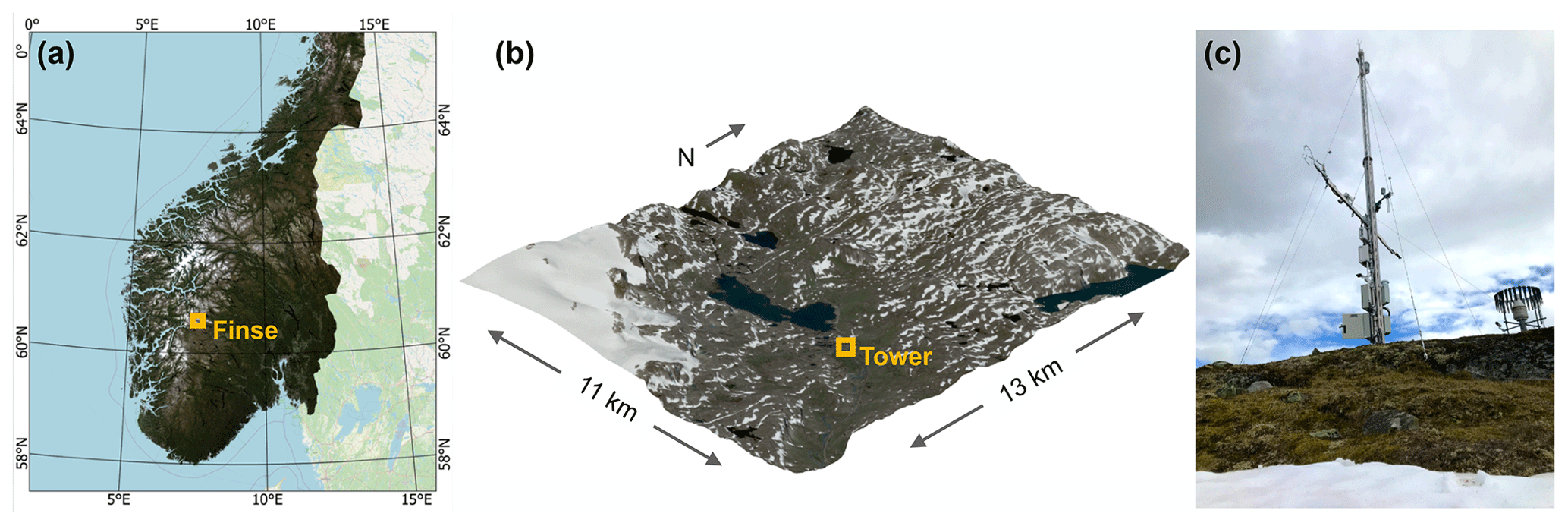
Figure 1Location and environmental setting of the Finse flux tower. (a) Location of Finse in southern Norway (background data contributed by Norge i Bilder and © Open Street Map). (b) Satellite image taken by Sentinel-2A on 31 August 2020 draped over an elevation model (DTM10 by Kartverket). (c) Image of the flux tower taken on 15 July 2020.
2.2 Flux measurements
Eddy covariance flux measurements of CO2 and water vapor were established at the Finse site (registered as NO-Fns in FLUXNET, Baldocchi et al., 2001) in 2016. Frequent technical problems with sensors and data loggers disrupted the first 2 years of operation, so the present study focuses on the period 2019–2021 with near-continuous flux data. The EC system consists of a CSAT3 three-dimensional sonic anemometer (Campbell Scientific, USA) and a Li-7200 closed-path infrared gas analyzer for CO2 and H2O mixing ratios (Li-Cor, USA). Both instruments are installed on the northern end of a horizontal boom at 4.4 m a.g.l. (Fig. 1c) and sampled at a frequency of 20 Hz. The Li-7200 gas analyzer uses a 71 cm long heated intake tube (6 W) with a flow rate of 15 L min−1.
We processed the EC raw data to 30 min flux estimates following the conventional EC methodology (Gu et al., 2012) using EddyPro version 6.2.0 (Li-Cor). We extract turbulent fluctuations from block averages, use an anemometer tilt correction by double rotation, a constant time lag compensation, and a high- and low-pass filter correction following Moncrieff et al. (2005) and Moncrieff et al. (1997), respectively. For quality control, we use statistical tests on the raw data proposed by Vickers and Mahrt (1997) and the flagging system proposed by Foken and Wichura (1996) to filter out flux estimates that are affected by instrument errors (e.g., rain or frost on the anemometer) or unfavorable micrometeorological conditions (e.g., lack of stationarity or turbulent mixing at low wind speeds). Following Vickers and Mahrt (1997), we estimate the number of spikes and drop-outs and also the absolute limits, amplitude resolution, skewness and kurtosis, and discontinuities for the pairs of raw data time series involved in the respective covariance-based flux estimates, and we discard data exceeding the thresholds proposed in the original paper. We also discard data with mean horizontal wind speeds below 1.5 m s−1, all fluxes with quality flag 2 in the scheme by Foken and Wichura (1996), and fluxes with quality flag 1 if they have relatively large magnitudes, i.e., above 1.0 µmol m−2 s−1 for NEE and 0.9 mmol m−2 s−1 for ET (corresponding approximately to the 40th percentile for both fluxes after filtering). After filtering the flux time series for unfavorable measurement conditions, we are left with 24 076 NEE and 22 708 ET valid half-hourly flux measurements, corresponding to 46 % and 43 % coverage of the entire period from 2019–2021, respectively.
2.3 Ancillary in situ measurements
There are a multitude of ancillary sensors on the Finse flux tower to quantify soil, surface, and atmospheric conditions during our flux measurements. Near-surface air temperature (Tair) is measured by a resistance temperature detector (PT-100) mounted in a radiation shield at 2 m a.g.l. Growing degree days (GDDs) are calculated from Tair according to its standard definition using a base temperature of 0 ∘C. The vapor pressure deficit (VPD) is derived from measurements of Tair and relative humidity (HMP155, Vaisala, Finland) mounted at 2 m a.g.l. Soil temperature (Tsoil) and soil volumetric water content (VWC) are measured at a depth of 8 cm (CS650, Campbell, USA). For incoming shortwave and longwave radiation (SWin and LWin, respectively) we use a ventilated and heated radiometer (CNR4, Kipp&Zonen, Netherlands) mounted on a south-pointing boom at 4 m a.g.l. The same sensor is used to measure surface broadband albedo. Snow depth (SD) is measured by a laser distance sensor (SHM30, Jenoptik, Germany) at a location about 4 m northeast of the tower. Skin surface temperature (Tsurf) is measured with an infrared radiometer (SI-411, Apogee, USA) at approximately the same location as the snow depth measurement. All these ancillary sensors are sampled every 10 s, filtered for corrupted measurements, and aggregated to 30 min average values. Due to data logger problems, approximately 2 % of the 30 min intervals lack valid local measurements in the period from 2019 to 2021. For atmospheric and surface variables, these short gaps are filled with estimates derived from a simple linear regression of the respective variable against its corresponding estimate from ERA5 atmospheric reanalysis data (Hersbach et al., 2020). Soil variables, which vary on longer timescales, are filled with a linear interpolation of neighboring measurements. The resulting time series are shown in Fig. S1 in the Supplement.
2.4 Satellite remote sensing
High-resolution satellite-based daily fractional snow-covered area (FSCA) and normalized difference vegetation index (NDVI) estimates are employed both as predictors in the flux gap-filling (Sect. 2.5) and to analyze the spatio-temporal links between snow melt-out and the presence of ecosystem types based on in situ vegetation mapping (Sect. 2.6). These estimates were obtained by merging and temporally gap-filling retrievals from multi-sensor multispectral satellite imagery covering the 3×3 km2 area around the Finse flux tower at a ground sampling distance of 10 m. For this purpose, we combine surface reflectance imagery (i.e., level-2 products) from both the twin Sentinel-2 satellites and the Landsat 8 satellite in the following six wavelength bands: blue (≃0.49 µm), green (≃0.55 µm), red (≃0.65 µm), near-infrared (≃0.85 µm), shortwave infrared 1 (≃1.6 µm), and shortwave infrared 2 (≃2.1 µm). The data were obtained from Google Earth Engine (Gorelick et al., 2017), which is a cloud-based platform that harvests these open datasets from the original data sources, namely Copernicus (Sentinel-2) and USGS (Landsat 8). The FSCA is retrieved using the spectral-unmixing approach described in Aalstad et al. (2020). The NDVI, which is commonly used as a proxy for surface greenness, leaf area, and vegetation development, is calculated according to its standard definition (Jia et al., 2003). To avoid artifacts in the satellite-based surface reflectance data that can occur due to clouds, we manually selected cloud-free scenes. This selection provided a total of 93 Sentinel-2 scenes and 20 Landsat 8 scenes for the entire study period, resulting in an average of around 4 cloud-free scenes per month. Note that Landsat 8 imagery, which has a slightly coarser (30 m) native resolution, was only used for days where no 10 m Sentinel-2 imagery was available. The combined stacks of cloud-free retrievals of FSCA and NDVI were independently interpolated in time for each pixel using Gaussian process regression (Rasmussen and Williams, 2005) with an exponential kernel and automatic relevance detection. The snow melt-out date was determined for each pixel as the first day with FSCA below 0.25.
Moderate-resolution satellite imagery with a longer temporal extent is used to build a multi-decadal climatology of the melt-out date of the seasonal snow cover around Finse that can help contextualize the melt-out dates during the study period (2019–2021). For this purpose, we use daily normalized difference snow index estimates from the MODerate resolution Imaging Spectroradiometer (MODIS) at 500 m spatial resolution to retrieve the FSCA based on a linear relationship (Salomonson and Appel, 2006) for all water years (September–August) from 2001–2021. MODIS is an optical satellite-based sensor currently on board two polar-orbiting satellites, namely Terra and Aqua. These measurements from the MODIS sensors include gaps that are mainly due to cloud cover. By merging two MODIS-based snow products from Terra (MOD10A1; Hall et al., 2015a) and Aqua (MYD10A1; Hall et al., 2015b), we are reducing these gaps for a given day. Subsequently, a temporal cloud gap-filling algorithm following Hall et al. (2019) is applied to this merged product to obtain gap-free daily FSCA estimates. For each pixel, snow melt-out dates are determined as the last day in a water year with FSCA greater than 0.25 during a period with at least 5 consecutive snow cover days. We averaged these estimates from the four closest MODIS pixels to the Finse tower to determine the snow melt-out dates at our site. To estimate the exceedance probability of the late snow melt-out in 2020 and to identify whether or not this year was an extreme year, we fit a beta distribution – a commonly used distribution with two shape parameters (α and β) for double-bounded random variables – to the melt-out dates from the MODIS dataset with the maximum likelihood method. Using gamma, logit-normal, and generalized extreme value distributions for the fit to the melt-out dates only has minimal influence on the resulting exceedance probability.
The FSCA dynamics estimated from the MODIS data agree qualitatively with a visual inspection of daily webcam imagery available at the Finse research station (https://www.finse.uio.no/news/webcam/, last access: 5 June 2023). We also evaluated the snow cover duration from the MODIS using the higher-resolution (Sentinel-2 and Landsat 8) retrievals as a reference during an overlap period (from 2017–2021) and found a close agreement with a root-mean-square error of 6 d and a correlation coefficient r of 0.98 for the 9 km2 study area.
2.5 Flux gap-filling
As gaps in the EC flux time series can occur systematically depending on environmental conditions, we use gap-filling to avoid biases in our annual flux budgets. To allow for a complex range of biogeochemical interactions, we developed a random forest regression model (Breiman, 2001; Kim et al., 2020) of the fluxes with 12 predictors quantifying the environmental conditions (Fig. S1 in the Supplement). Ten of these predictors are measured directly at the flux tower, as described in Sect. 2.3, while two additional ones – the fractional snow-covered area (FSCA) and normalized difference vegetation index (NDVI) – are derived from remote sensing (Sect. 2.4). These 12 predictors are chosen to provide a robust and detailed characterization of each 30 min flux period, including soil, surface, and atmospheric conditions. Some of the predictors are correlated, at least in some parts of the predictor space, which must be considered when interpreting the predictor importance obtained from the random forest regression model (Gregorutti et al., 2017). Since even highly correlated predictor pairs may capture nuances of potentially important flux dynamics, we chose to use their information in our gap-filling routine despite the partial redundancy (see discussion in Sect. 4.2). Note that the resulting flux estimates from the random forest regression model are only used to fill gaps in the flux time series, i.e., not to replace valid flux measurements.
The setting of the landscape at the Finse flux tower favors a bi-modal distribution of wind directions along an east–west axis. To account for the potentially different surface cover of the easterly and westerly footprint, we split the dataset into the two main wind directions (wind directions above and below 180∘) and gap-filled these subsets separately. Such splits are common to prevent annual flux budgets from depending on the distribution of the wind directions (Griebel et al., 2016).
We use the random forest regression implementation provided by the scikit-learn Python module (Pedregosa et al., 2011), with 2000 trees per forest and otherwise default parameters. The random forest regression model is trained on valid EC flux measurements that have passed quality controlling. To assess potential overfitting that would limit the generalization of the model to unobserved data, we also trained separate models using only 80 % of our valid dataset, keeping 20 % for testing through independent evaluation (validation). The coefficients of determination of these random forest models ranged between across the two flux types (NEE and ET) and wind sectors (Table S2 in the Supplement). We also tested the reduction of model complexity by limiting the number of predictors that each tree is randomly assigned or by reducing the maximally allowed depth of each tree. However, the resulting evaluation statistics indicated that overfitting is not a problem for our case, with more than 1000 times more data points than predictors.
2.6 Footprint characterization by ecosystem types
The footprint function of each valid 30 min flux is estimated based on friction velocity (u*), wind direction, Obukhov length (L), and cross-wind variance (vvar) (all from EC measurements), as well as boundary layer height (linearly interpolated estimates from single-level ERA5 hourly data) and a tundra-typical roughness length of 1 cm following the flux footprint model by Kljun et al. (2015). The resulting 1×1 m2 resolution flux weight maps are clustered by ecosystem type using a map of the area created in situ by Bryn and Horvath (2020) at a mapping scale of 1:5 000 to assess the flux contributions of different surfaces. The implemented Nature in Norway (NIN) hierarchical mapping system (Halvorsen et al., 2020) consists of a total of 741 minor and 92 major ecosystem types. Of these, 43 minor and 13 major types are found in the study area at Finse. For the purpose of this study, the ecosystem types are further reclassified into seven main type categories (Table S1 in the Supplement). Fens comprise all open mires with peat-dominated ground layers that, in addition to rainwater, are also fed by groundwater that has been in contact with the mineral soil. Flood plains include open alluvial sediments regulated by balancing sedimentation and erosion. Mountain heathlands are characterized as naturally open ecosystems above the climatic forest limit, dominated by dwarf shrubs (Empetrum nigrum, Salix spp., and ericaceous species), herbs, graminoids, and bryophytes. Exposed ridges (and lichen heathlands) are confined to convex terrain and areas that lack permanent snow cover in winter during periods with extremely low temperatures, freeze-drying conditions, and physical wind abrasion, dominated by specialized stress-tolerant lichens, mosses, and vascular plants. Moss-dominated snowbeds are characterized by a combination of shortened growing seasons due to prolonged snow cover and shelter of the vegetation against low temperatures and wind abrasion during winter. Moderate snowbeds occupy the lower lee-sides of the topographical ridge–snowbed gradient in alpine and arctic areas, while late and extreme snowbeds can be found at the lowest part of the topographical depressions, where snow does not completely melt each year. This ecosystem-type map allows for a detailed analysis of the high-resolution snow cover maps derived from satellite remote sensing (Sect. 2.4) to explore dependencies between snow melt-out date and the presence of ecosystem types.
2.7 Synoptic patterns
To characterize the atmospheric circulation pattern during the heavy snowfall in 2020 compared to other years, we analyze the correlation between wintertime precipitation and the Scandinavian Pattern Index (SCA, referred to as Eurasia-1 pattern by Barnston and Livezey, 1987) estimated from monthly ERA5 data using the KNMI Climate Explorer (Trouet and Van Oldenborgh, 2013). Similarly to the North Atlantic Oscillation Index, which has already been linked to variability in snow water equivalent in Norway (Skaugen et al., 2012), the Scandinavian Pattern Index is based on the surface air pressure difference between the subtropical and subpolar regions. We exemplify the resulting patterns using February as a month in the middle of the snow season that typically features large snowfall events.
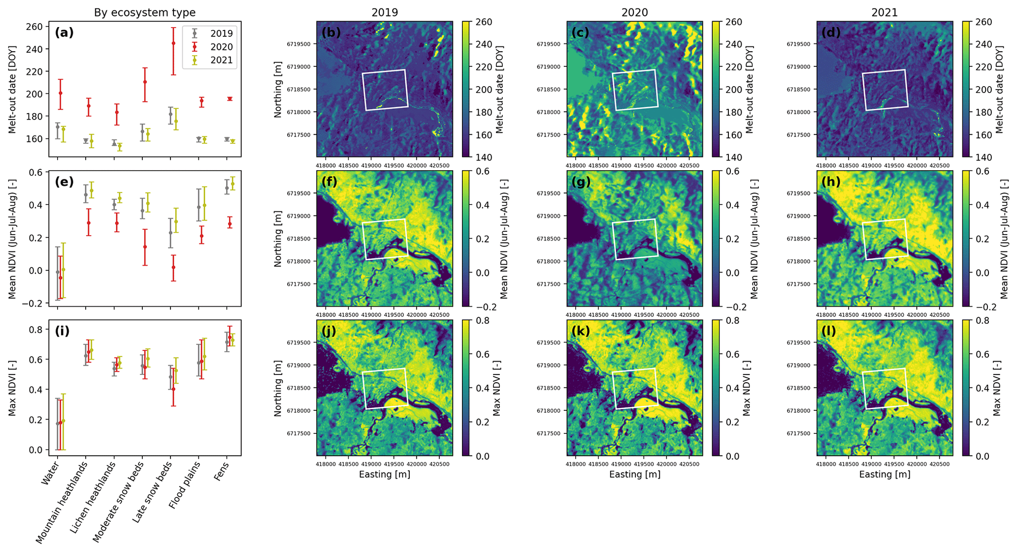
Figure 2Remotely sensed melt-out dates and NDVI statistics from the combined Sentinel-2 and Landsat 8 retrievals for 2019, 2020, and 2021. Left: clustered into different ecosystem types. Dots represent mean values, and error bars represent the inter-quartile ranges of the distributions within each ecosystem type. Middle and right: maps for the 9 km2 area around the flux station. The white rectangle represents the area around the flux tower where ecosystem-type mapping and clustering was performed (same as in Fig. 4a).
3.1 Snow–vegetation interactions at Finse
Figure 2a shows the results of the spatial clustering of remotely sensed melt-out dates from the combined Sentinel-2 and Landsat 8 retrievals to the ecosystem-type map. Different ecosystem types are associated with markedly different snow melt-out characteristics. While fens and floodplains melt out relatively simultaneously (i.e., with small within-ecosystem-type variance), mountain and lichen heathlands melt out slightly more variably. Moderate and late snowbeds melt out most variably and, on average, 1 to 2 months after the other ecosystem types. Figure 2a–d show that all 3 years exhibit similar relative melt-out patterns, but 2020 had considerably later overall melt-out dates. This difference can largely be attributed to differences in snow accumulation in winter and spring, exemplified by a maximum snow depth of 205 cm in 2020 compared to 52 cm in 2019 and 70 cm in 2021, as measured at the flux tower (Fig. S1 in the Supplement).
The relative response of the vegetation development to the snow cover is assessed by our NDVI estimates. Figure 2e and i show that fens and mountain heathlands have the highest and similar mean and maximum NDVI, followed by flood plains, lichen heathlands and moderate snow beds (with similar NDVI statistics), and finally late snow beds. Averaged across the 3 summer months, NDVI was lower in 2020 compared to 2019 and 2021 (Fig. 2e–h), which can be explained by the longer snow duration because snow-covered areas typically have low negative NDVI values close to zero. The maximum NDVI of each ecosystem type, however, was very similar in all years (Fig. 2h and i). This robustness of annual-maximum NDVI indicates that, while the summertime-average leaf area and greenness was reduced in the snow-rich year of 2020, the peak NDVI still reached the same level as in the other years. The only exception are late snowbeds (and to a smaller degree moderate snowbeds), where the extreme snow accumulation of 2020 noticeably inhibited vegetation growth. The effect of snow melt-out date on annual-maximum NDVI can also be seen from the spatial anti-correlation of these variables in the 9 km2 satellite area, which was on average and was especially strong in 2020 ( in 2019, in 2020, and in 2021).
Most of the snowpack at Finse built up in only a few major precipitation events, and almost half of the maximum snow depth accumulated during two snowfall events in the winter months (Fig. S1 in the Supplement). The intensity of wintertime precipitation in southern Norway can, in part, be explained by the synoptic atmospheric circulation pattern, as exemplified by the large anti-correlation between the Scandinavian Pattern Index and February precipitation (Fig. 3a). In winter 2020, the Scandinavian Pattern Index for February exhibited its lowest value in the ERA5 record (1950–2021), while 2019 and 2021 were close to the mean value (Fig. 3b). The associated large snowfall events in the winter of 2020 contributed to the extremely late snow melt-out (Fig. 3c). The beta distribution fitted to the melt-out dates shows that 2020 falls in the 92nd percentile of the distribution, rendering 2020 an extremely snow-rich year. The snow melt-out date in 2020 ranked second in this time series of 21 years (only exceeded in 2015).
3.2 Flux dynamics in the two footprints
Figure 4 provides a characterization of the footprint of the EC flux measurements during the period 2019–2021 in terms of the weighted contribution of each ecosystem type. The footprint of each flux-averaging period (30 min), as well as the average footprint of the entire flux time series, receives contributions from a broad mixture of ecosystem types. Overall, snowbed surfaces have a footprint-weighted contribution of 30 % to the total footprint area, followed by heathlands (29 %), water surfaces (25 %), fens and flood plains (14 % together) (Table S1 of the Supplement). The bi-modal distribution of wind directions seen in Fig. 4b aligns along the east–west direction of the valley, facilitating the binary separation between the easterly and the westerly footprint in the flux analysis. The easterly footprint is characterized by a larger fraction of water surfaces and late snowbeds, while the westerly footprint has a larger fraction of fens and moderate snowbeds, with a denser vegetation cover. These two footprints are therefore treated separately to reduce the confounding effects of the spatial and temporal variability of the measured fluxes.
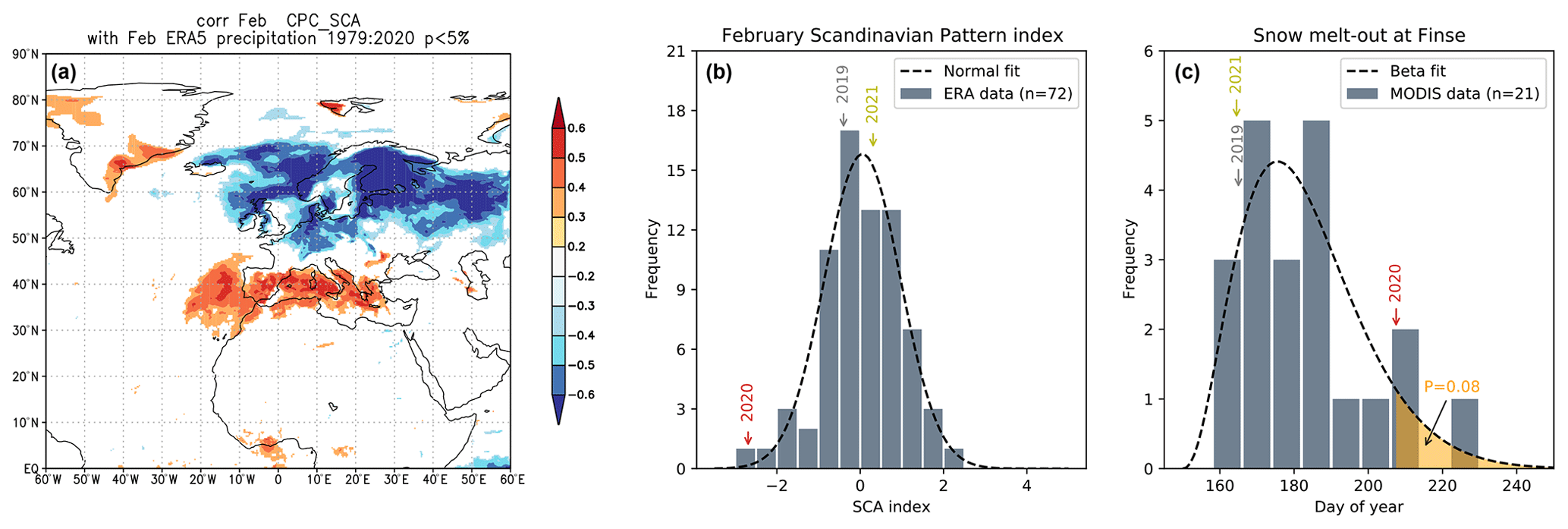
Figure 3Synoptic atmospheric circulation patterns and snow cover statistics. (a) Correlation map between Scandinavian Pattern Index (SCA) and precipitation in February indicating a strong association in northern Europe. (b) Histogram of all February values of the Scandinavian Pattern Index in the ERA5 period (1950–2021) along with the fitted normal distribution. (c) Histogram of the snow melt-out day at Finse derived from MODIS data (2001–2021) along with the fitted maximum likelihood beta distribution (shape parameters α=3.42 and β=18.98).
The net ecosystem exchange of the westerly footprint (Fig. 5a) shows both diurnal and annual cycles, as may be expected for a summer active, high-latitude tundra ecosystem. The winter and spring seasons are characterized by small but steady CO2 releases of about 0.1 µmol m−2 s−1. The start of the growing season with daily average CO2 uptake fluxes occurs 2 weeks after the estimated day of snowmelt. Summer nights show the largest CO2 releases, but daytime CO2 uptake during summer exceeds these nighttime releases in magnitude by a factor of about 5. These flux dynamics are similar across the years, with the important difference of a much shorter growing season in 2020. The net ecosystem exchange of the easterly footprint (not shown) exhibits the same dynamics as the westerly footprint, with a correlation coefficient of r=0.92 between the two, albeit with a smaller flux magnitude (slope of linear regression of 0.61). The predictor importance of the random forest analysis (Fig. 5b) indicates that shortwave incoming radiation, surface temperature, and NDVI are the main controls on NEE in both footprints.
Evapotranspiration shown for the westerly footprint in Fig. 5c also highlights different dynamics during the growing season compared to the rest of the year. During winter and spring, as well as during summer nights, small evaporation, sublimation, and condensation fluxes occur interchangeably, depending on the physical state of the ground and the surface layer air. Spring 2020 had a period where condensation dominated daytime fluxes, but compared to summertime ET, these fluxes were relatively small. For daytime periods during the growing season, fluxes can be 1 order of magnitude larger and hence dominate the annual ET budget. As seen for NEE, ET dynamics are similar across the years but with reduced fluxes in the growing season of 2020. In the easterly footprint, ET largely follows the same dynamics as in the westerly footprint (with a correlation coefficient of r=0.89) but with a smaller flux magnitude (slope of linear regression of 0.58). The predictor importance for ET (Fig. 5d) indicated that vapor pressure deficit, surface temperature, and incoming shortwave radiation act as the most important drivers for both footprints.
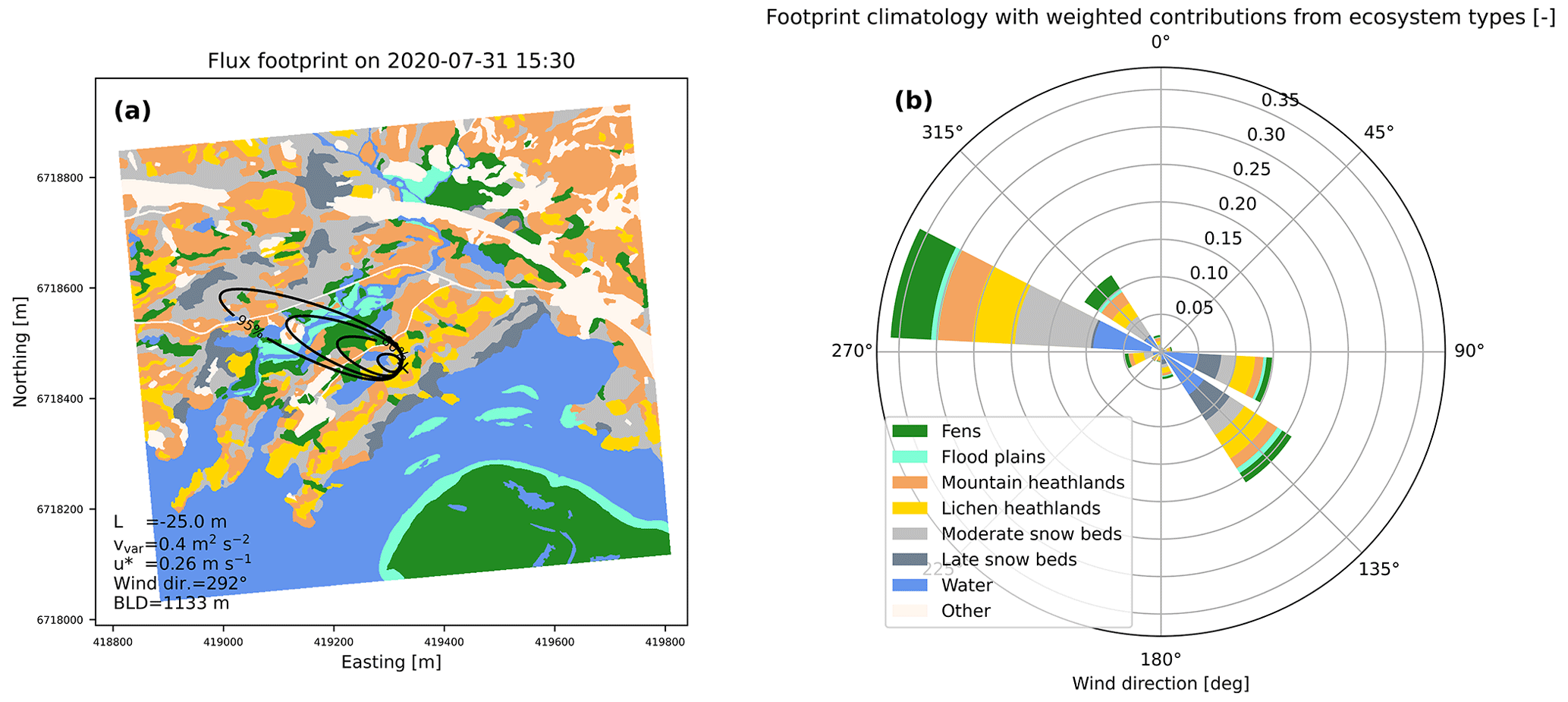
Figure 4Flux footprint characterization. (a) Example of a footprint estimate for one flux-averaging period during daytime summer conditions with unstable stratification. The background map shows the seven main ecosystem-type categories, while the black lines show the contours of the 50 %, 80 %, 90 %, and 95 % cumulative footprints (from inside to outside), respectively. (b) Integrated footprint function averaged over all valid NEE measurements during 2019–2021 and plotted by the corresponding wind sectors. Colors indicate the footprint-weighted contribution of each ecosystem type. The weights sum up to about 0.91, corresponding to the fraction of the EC footprint that is classified by the ecosystem-type map.
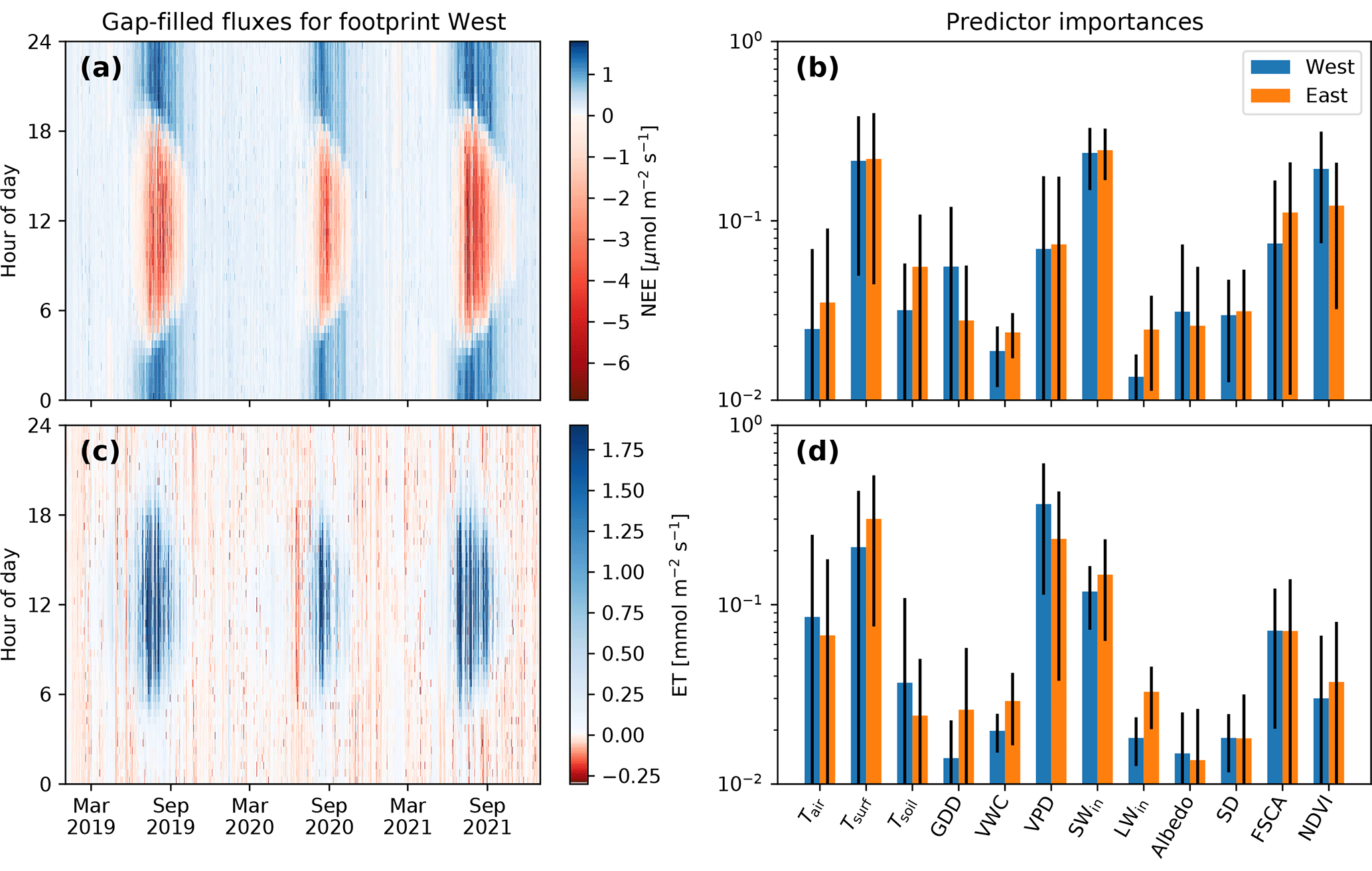
Figure 5Flux dynamics and drivers. (a, c) Gap-filled NEE and ET as fingerprint plots for the westerly footprint. (b, d) Predictor importance of the random forest regression models of both the easterly and westerly footprints plotted on a logarithmic scale. Black error bars indicate the standard deviation across the 2000 trees in the respective random forests.
3.3 NEE and ET budgets
Figure 6 shows the cumulative NEE and ET of both footprints for each year. For NEE, more than 9 months of the year typically feature small emissions of CO2. In 2019 and 2021, these emissions were exceeded by an intense CO2 uptake during the growing season, rendering the site a moderate annual carbon sink of between −6 and −31 gC m−2 yr−1 in both footprints (see Table S3 in the Supplement for detailed growing-season statistics). In the extreme-snow year 2020, however, the growing-season CO2 assimilation was too small to offset wintertime emissions, causing the annual carbon balance to become positive (carbon source) in both footprints (between 20 and 34 gC m−2 yr−1). For the westerly footprint, the effect of a shortened growing season even made the ecosystem a stronger annual carbon source than it was a sink in the other 2 years. The large snow volumes in 2020 not only delayed the start of the growing season but also markedly prevented ground freezing in wintertime (Fig. S1 in the Supplement). The resulting higher soil temperatures allow for increased microbial activity in the soil, which can explain the slightly larger wintertime CO2 emissions observed in 2020. Summer 2021 is characterized by larger CO2 uptake fluxes compared to 2019, which may be caused by slightly higher GDDs, resulting in slightly higher NDVI values in 2021 (Fig. S1 in the Supplement). The end of the growing season, when the ecosystem returns to being a net daily CO2 source, occurred between 5 and 26 September and is associated with a fall in NDVI.
The ET loss is largely dominated by growing-season fluxes. The annual ET loss is larger in the more densely vegetated westerly footprint but is still less than 10 % of total annual precipitation in both footprints. The ET contribution to the water balance is particularly low in 2020, when the short growing season resulted in a decrease in annual ET of almost 50 %. Collectively, these observations are consistent with the notion that a large portion of ET stems from transpiration through stomatal fluxes as opposed to non-stomatal evaporation from bare ground or interception storage.
The carbon uptake and ET loss integrated over the growing season can be used to estimate the integrated water-use efficiency (WUE) of the ecosystem, also termed WUE of productivity. This comparison shows that, while both footprint areas are characterized by similar WUE in 2019 and the extreme-snow year 2020 (ranging between 1.20 and 1.37 µmol-CO2 mmol-H2O−1), the following year of 2021 showed a marked increase in WUE to values between 1.77 and 1.96 µmol-CO2 mmol-H2O−1 (Table S3 in the Supplement). On average, these differences correspond to an increase in ecosystem water-use efficiency of about 47 %.
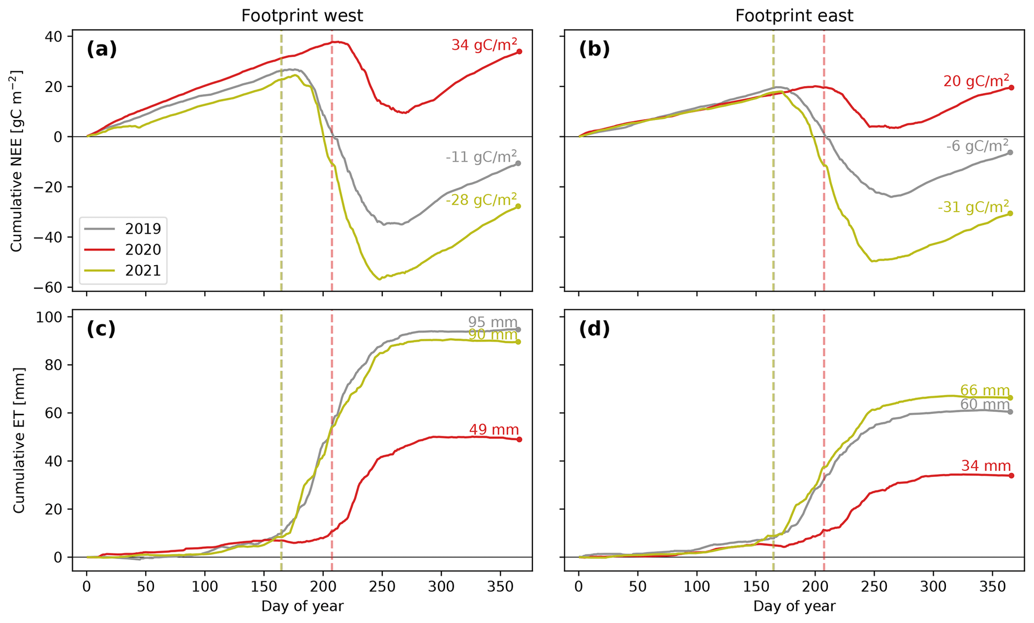
Figure 6Cumulative sums of NEE (a, b) and ET (c, d) for different footprint areas (columns) and years (lines). Stipulated lines indicate the snow melt-out date estimated from MODIS (which was equal in 2019 and 2021).
4.1 Snow cover anomalies as extreme events in alpine ecosystems
The ecology of alpine tundra along the Scandinavian mountain chain is strongly regulated by the spatial distribution and longevity of the snow cover (Dahl, 1956; Odland and Munkejord, 2008; Niittynen and Luoto, 2018), as corroborated by the persistent linkage between snow melt-out date and ecosystem type in the present study (Fig. 2a). Compared to the boreal region, the alpine tundra in Norway is less affected by disturbances from wildfires (Jolly et al., 2015), heat waves (Ciais et al., 2005), or insect outbreaks (Heliasz et al., 2011). Although there is a history of free-ranging domestic animals (Ross et al., 2016) and reindeer (Kolari et al., 2019), as well as cycles of rodent population outbreaks (Kausrud et al., 2008), snow cover anomalies are likely to be driving the most consequential structural shifts of this ecosystem’s functioning. The identified link between snowfall intensity and the Scandinavian Pattern Index of the synoptic atmospheric circulation provides a new perspective for our understanding of snow cover anomalies at Finse. The associated hydrological and biochemical consequences in areas with delayed snow melt-out can include enhanced groundwater recharge and subsequent discharge (Jasechko et al., 2014), wetter soils, higher pH, and more nutrients in the soils (Moriana-Armendariz et al., 2022). Our flux measurements clearly indicate the direct reduction of NEE and ET in extreme-snow years. Perhaps somewhat surprisingly, our NDVI analysis reveals that the tundra vegetation still developed the same leaf area and greenness in the extreme-snow year of 2020 compared to the other 2 years. In areas with short growing seasons, such as at Finse, a quick development of new leaves on deciduous shrubs is needed to reduce the risk of missing the opportunity to grow. This quick leaf development is accomplished through the mobilization of below-ground stored assimilates from the previous year (Karlsson, 1985; Körner and Renhardt, 1987; Tonjer et al., 2021). Although beyond the scope of this study, such below-ground responses could be explored using factorial experiments with minirhizotron tubes in climate chambers (Blume-Werry et al., 2019). Further, in order to maximize leaf area, leaves that are pre-planned in buds must not be injured by low winter temperatures or frost spells after bud break (Wipf et al., 2009). In our study, the late melt-out in 2020 came after a relatively successful growing season in 2019, probably securing assimilate storage and well-developed buds. The shoots of 2020 came out late, thus probably avoiding frost spells. Accordingly, NDVI reached a high maximum level, although the remainder of the growing season was too short to secure a negative NEE that year. So if extreme snow accumulations become more frequent, the observed reduction of growing-season carbon assimilation could provide a mechanism for a trajectory for expanding snowbeds and reduced vascular plant cover in some ecosystem types in alpine regions, which would slow down the widely observed advances of birch trees to alpine regions and the shrubification of tundra areas.
In the growing season of 2021, our flux measurements show a marked increase in the WUE of the ecosystems in both footprint areas. Compared to 2019, NDVI, GDDs, and NEE were higher in 2021, whereas ET stayed approximately the same (see Fig. S1 and Table S3 in the Supplement). Since our measurements do not suggest a clear mechanism for this increase in WUE, it remains an open question whether it is due to a carry-over effect of the previous snow-rich year or is the direct response to a slightly higher air temperature (as suggested by Wang et al., 2020) or lower volumetric water content in the soil due to less frequent precipitation (Fig. S1 in the Supplement).
The Finse area typically features a several-months-long ablation season with patchy snow cover (Aas et al., 2017). The main drivers of melt-out variability are likely differences in wind exposition and surface orientation with respect to prevailing wind directions and insolation. Likewise, wind-driven snowmelt by heterogeneous sensible heat fluxes can play a decisive role for snowmelt dynamics (van der Valk et al., 2022). While our partitioning of snow patchiness into within- and between-ecosystem-type variability (Fig. 2a) comes with some sensitivity to our choice of merging the minor ecosystem types, it may offer new insights into the drivers of snowmelt and discharge generation on the landscape scale. In this context, it would also be interesting to investigate the thermal impact of (relatively warm) groundwater upwelling (e.g., in streams or in the fens) on snowmelt and associated changes such as soil moisture and NEE. A companion paper to the present work assesses how changing snow patterns affect the hydrology and aquatic biogeochemical cycling, including greenhouse gas dynamics, in the Finse area.
4.2 Eddy covariance measurements in mountainous environments
Mountainous topography can create characteristic boundary layer flow features due to, e.g., orographic gravity waves and cross-valley circulation cells that add effective transport mechanisms to the otherwise-isotropic turbulent mixing (Lehner and Rotach, 2018; Adler et al., 2021). At Finse, the nearby Hardangerjøkulen Glacier is likely to induce a secondary circulation pattern due to strong surface temperature gradients, especially during summertime. Such mesoscale disturbances can add noise and even systematic biases to EC flux estimates, since they are not accounted for in the fundamental equation of EC (Gu et al., 2012). One manifestation of such problems can be seen in the non-closure of the surface energy budget that is typically of the order of 20 % (Wilson et al., 2002) and that increases with landscape heterogeneity (Stoy et al., 2013). Ramtvedt and Pirk (2022) showed that net radiation varies significantly over different surfaces around the Finse flux tower. However, even after correcting for these differences, the energy imbalance at Finse was still about 50 % – similar to values found at other alpine sites (Rotach et al., 2004). Vertical temperature gradient measurements at our tower (Fig. S2 in the Supplement) indicate stable stratification for about 83 % of the period 2019–2021, with temperature gradients between the 2 and 10 m levels as high as 6 ∘C during low-wind conditions. The resulting surface-based temperature inversions and stable boundary layer flows are known to feature flux divergences that can, in part, explain the observed energy imbalances (Mahrt et al., 2018). It is, however, still unclear to what extent this problem affects other flux estimates such as NEE. Adapted data-processing techniques (Sievers et al., 2015) or alternative measurements using fiber optics (Fritz et al., 2021) or drones (Pirk et al., 2022) could be employed to further investigate the surface energy imbalance at Finse, ideally in combination with other mountainous sites.
4.3 Statistical flux gap-filling
The random forest regression model for flux gap-filling performed well for our dataset, yielding generally low root-mean-square errors and high values of the coefficient of determination ( in test datasets; see Table S2 in the Supplement). Unlike other commonly used gap-filling algorithms like marginal distribution sampling (Reichstein et al., 2005), where gaps are filled with average fluxes measured during similar conditions within a moving time window, the random forest model implicitly models the nonlinear biogeo-chemical and biogeo-physical interactions that give rise to fluxes. The disadvantage is that random forest models cannot extrapolate to regions of the input–output space that are outside the observed range. For near-continuous datasets, such as our NEE and ET fluxes, this is not a critical limitation, but datasets with larger gaps during extreme environmental conditions would be more challenging to gap-fill with random forest models. While the predictor importance hints towards the underlying processes and can help develop new hypotheses about biogeo-chemical and biogeo-physical interactions, their interpretation is complicated by correlations among the predictors, as is common for statistical and machine learning models with multiple predictors (Gregorutti et al., 2017). The predictor importance in our flux model is in good agreement with our prior expectations about the flux drivers. At the same time, our analysis emphasizes the need for high-quality ancillary measurements nearby flux towers. In accordance with the no-free-lunch theorems of optimization (Wolpert and Macready, 1997), a range of different statistical and machine learning models would likely fit the data equally well. Bayesian additive regression tree models (Chipman et al., 2010), for example, appear to be a promising technique that would also directly estimate the statistical uncertainty of gap-filled fluxes. For our estimation of annual budgets, however, the uncertainty of statistical gap-filling is typically small compared to the systematic uncertainty of the EC flux estimates (Pirk et al., 2017).
We investigated snow–vegetation–atmosphere interactions at the Finse site in alpine Norway by analyzing CO2 and water vapor eddy covariance flux measurements in combination with ground-based ecosystem-type mapping and satellite remote sensing. Our analysis shows the consistencies and dependencies between these fluxes, ecosystem types, and the snow cover duration in 3 consecutive years. The spatial variability in the melt-out dates of different ecosystem types (Fig. 2a) and the temporal response of the ecosystem-scale NEE and ET to extreme-snow years (Fig. 6) represent a complementary manifestation of snow–vegetation–atmosphere interactions at different scales that determine ecosystem functioning at the Finse site. The year 2020 is identified as an extremely snow-rich year associated with a record-low SCA index for February, which reduced the total annual evapotranspiration to 50 % and reduced the growing-season carbon assimilation to turn the ecosystem from a moderate annual carbon sink (−31 to −6 gC m−2 yr−1) to an even stronger source (34 to 20 gC m−2 yr−1). The ecosystem water-use efficiency increased by about 47 % in the year after the extreme-snow year, but longer flux monitoring is needed to assess if this response constitutes a persistent structural shift to the extremely short growing season. As the alpine tundra in Norway is less affected by disturbances such as wildfires, insect outbreaks, or heat waves, our analysis suggests that snow cover anomalies drive the most consequential short-term responses in this ecosystem's functioning.
The ecosystem-type map is available on GitHub (https://github.com/geco-nhm/NiN_Finse, Horvath, 2023). Gap-filled flux data and remote sensing results for FSCA and NDVI are available at https://doi.org/10.5281/zenodo.7566641 (Pirk et al., 2023).
The supplement related to this article is available online at: https://doi.org/10.5194/bg-20-2031-2023-supplement.
Conceptualization: NP, KA, PH, and AB. Data curation: NP, KA, YAY, AV, PH, and AB. Formal analysis: NP, KA, YAY, and PH. Funding acquisition: NP, AB, SW, TKB, FS, and LMT. Writing – original draft preparation: NP, KA, and PH. Writing – review and editing: NP, KA, YAY, AV, ALP, AVV, PH, AB, SW, TKB, FS, and LMT.
The contact author has declared that none of the authors has any competing interests.
Publisher’s note: Copernicus Publications remains neutral with regard to jurisdictional claims in published maps and institutional affiliations.
This work is a contribution to the strategic research initiative LATICE (Faculty of Mathematics and Natural Sciences, University of Oslo, project no. UiO/GEO103920), the Center for Biogeochemistry in the Anthropocene, and the Center for Computational and Data Science. The study contains Landsat data (courtesy of the US Geological Survey) and modified Copernicus Sentinel data (year 2019, 2020, 2021) obtained from the Google Earth Engine. MODIS snow cover products MOD10A1 and MYD10A1 were obtained from NASA National Snow and Ice Data Center Distributed Active Archive Center (NSIDC DAAC).
This research has been supported by the Norges Forskningsråd (grant nos. 301552, 294948, and 323945).
This paper was edited by Paul Stoy and reviewed by Manuel Helbig and one anonymous referee.
Aalstad, K., Westermann, S., and Bertino, L.: Evaluating Satellite Retrieved Fractional Snow-Covered Area at a High-Arctic Site Using Terrestrial Photography, Remote Sens. Environ., 239, 111618, https://doi.org/10.1016/j.rse.2019.111618, 2020. a
Aas, K. S., Gisnås, K., Westermann, S., and Berntsen, T. K.: A Tiling Approach to Represent Subgrid Snow Variability in Coupled Land Surface–Atmosphere Models, J. Hydrometeorol., 18, 49–63, https://doi.org/10.1175/JHM-D-16-0026.1, 2017. a
Adler, B., Gohm, A., Kalthoff, N., Babić, N., Corsmeier, U., Lehner, M., Rotach, M. W., Haid, M., Markmann, P., Gast, E., Tsaknakis, G., and Georgoussis, G.: CROSSINN: A Field Experiment to Study the Three-Dimensional Flow Structure in the Inn Valley, Austria, Bull. Am. Meteorol. Soc., 102, E38–E60, https://doi.org/10.1175/BAMS-D-19-0283.1, 2021. a
Arias, P., Bellouin, N., Coppola, E., et al.: Climate Change 2021: The Physical Science Basis, Contribution of Working Group14 I to the Sixth Assessment Report of the Intergovernmental Panel on Climate Change, Technical Summary, Cambridge University Press, Cambridge, United Kingdom and New York, NY, USA, 33–144, https://doi.org/10.1017/9781009157896.002, 2021. a
Baldocchi, D., Falge, E., Gu, L., Olson, R., Hollinger, D., Running, S., Anthoni, P., Bernhofer, C., Davis, K., Evans, R., Fuentes, J., Goldstein, A., Katul, G., Law, B., Lee, X., Malhi, Y., Meyers, T., Munger, W., Oechel, W., Paw, K. T., Pilegaard, K., Schmid, H. P., Valentini, R., Verma, S., Vesala, T., Wilson, K., and Wofsy, S.: FLUXNET: A New Tool to Study the Temporal and Spatial Variability of Ecosystem–Scale Carbon Dioxide, Water Vapor, and Energy Flux Densities, Bull. Am. Meteorol. Soc., 82, 2415–2434, https://doi.org/10.1175/1520-0477(2001)082<2415:FANTTS>2.3.CO;2, 2001. a
Baldocchi, D. D.: How Eddy Covariance Flux Measurements Have Contributed to Our Understanding of Global Change Biology, Glob. Change Biol., 26, 242–260, https://doi.org/10.1111/gcb.14807, 2020. a
Barnston, A. G. and Livezey, R. E.: Classification, Seasonality and Persistence of Low-Frequency Atmospheric Circulation Patterns, Mon. Weather Rev., 115, 1083–1126, https://doi.org/10.1175/1520-0493(1987)115<1083:CSAPOL>2.0.CO;2, 1987. a
Beigaitė, R., Tang, H., Bryn, A., Skarpaas, O., Stordal, F., Bjerke, J. W., and Žliobaitė, I.: Identifying Climate Thresholds for Dominant Natural Vegetation Types at the Global Scale Using Machine Learning: Average Climate versus Extremes, Glob. Change Biol., 28, 3557–3579, https://doi.org/10.1111/gcb.16110, 2022. a
Bintanja, R. and Andry, O.: Towards a Rain-Dominated Arctic, Nat. Clim. Change, 7, 263–267, https://doi.org/10.1038/nclimate3240, 2017. a
Blume-Werry, G., Milbau, A., Teuber, L. M., Johansson, M., and Dorrepaal, E.: Dwelling in the Deep – Strongly Increased Root Growth and Rooting Depth Enhance Plant Interactions with Thawing Permafrost Soil, New Phytol., 223, 1328–1339, https://doi.org/10.1111/nph.15903, 2019. a
Breiman, L.: Random Forests, Mach. Learn., 45, 5–32, https://doi.org/10.1023/A:1010933404324, 2001. a
Bryn, A. and Horvath, P.: Kartlegging Av NiN Naturtyper i Må lestokk 1:5000 Rundt Flux-Tå rnet Og På Hansbunuten, Finse (Vestland), Naturhistorisk museum, Universitetet i Oslo, ISBN: 978-82-7970-122-4, https://doi.org/10.13140/RG.2.2.35946.75205, 2020. a
Carrillo-Rojas, G., Silva, B., Rollenbeck, R., Célleri, R., and Bendix, J.: The Breathing of the Andean Highlands: Net Ecosystem Exchange and Evapotranspiration over the Páramo of Southern Ecuador, Agr. Forest Meteorol., 265, 30–47, https://doi.org/10.1016/j.agrformet.2018.11.006, 2019. a
Chipman, H. A., George, E. I., and McCulloch, R. E.: BART: Bayesian Additive Regression Trees, Ann. Appl. Stat., 4, 266–298, https://doi.org/10.1214/09-AOAS285, 2010. a
Christensen, T. R., Lund, M., Skov, K., Abermann, J., López-Blanco, E., Scheller, J., Scheel, M., Jackowicz-Korczynski, M., Langley, K., Murphy, M. J., and Mastepanov, M.: Multiple Ecosystem Effects of Extreme Weather Events in the Arctic, Ecosystems, 24, 122–136, https://doi.org/10.1007/s10021-020-00507-6, 2021. a
Ciais, P., Reichstein, M., Viovy, N., Granier, A., Ogée, J., Allard, V., Aubinet, M., Buchmann, N., Bernhofer, C., Carrara, A., Chevallier, F., De Noblet, N., Friend, A. D., Friedlingstein, P., Grünwald, T., Heinesch, B., Keronen, P., Knohl, A., Krinner, G., Loustau, D., Manca, G., Matteucci, G., Miglietta, F., Ourcival, J. M., Papale, D., Pilegaard, K., Rambal, S., Seufert, G., Soussana, J. F., Sanz, M. J., Schulze, E. D., Vesala, T., and Valentini, R.: Europe-Wide Reduction in Primary Productivity Caused by the Heat and Drought in 2003, Nature, 437, 529–533, https://doi.org/10.1038/nature03972, 2005. a
Dahl, E.: Rondane, I kommisjon hos Aschehoug, 1956. a
Derksen, C. and Brown, R.: Spring Snow Cover Extent Reductions in the 2008–2012 Period Exceeding Climate Model Projections: SPRING SNOW COVER EXTENT REDUCTIONS, Geophys. Res. Lett., 39, L19504, https://doi.org/10.1029/2012GL053387, 2012. a
Easterling, D. R., Meehl, G. A., Parmesan, C., Changnon, S. A., Karl, T. R., and Mearns, L. O.: Climate Extremes: Observations, Modeling, and Impacts, Science, 289, 2068–2074, https://doi.org/10.1126/science.289.5487.2068, 2000. a
Erlandsen, H. B., Beldring, S., Eisner, S., Hisdal, H., Huang, S., and Tallaksen, L. M.: Constraining the HBV Model for Robust Water Balance Assessments in a Cold Climate, Hydrol. Res., 52, 356–372, https://doi.org/10.2166/nh.2021.132, 2021. a
Foken, T. and Wichura, B.: Tools for Quality Assessment of Surface-Based Flux Measurements, Agr. Forest Meteorol., 78, 83–105, https://doi.org/10.1016/0168-1923(95)02248-1, 1996. a, b
Frei, E. R. and Henry, G. H.: Long-Term Effects of Snowmelt Timing and Climate Warming on Phenology, Growth, and Reproductive Effort of Arctic Tundra Plant Species, Arct. Sci., 8, 700–721, https://doi.org/10.1139/as-2021-0028, 2022. a
Fritz, A. M., Lapo, K., Freundorfer, A., Linhardt, T., and Thomas, C. K.: Revealing the Morning Transition in the Mountain Boundary Layer Using Fiber-Optic Distributed Temperature Sensing, Geophys. Res. Lett., 48, e2020GL092238, https://doi.org/10.1029/2020GL092238, 2021. a
Gisnås, K., Westermann, S., Schuler, T. V., Litherland, T., Isaksen, K., Boike, J., and Etzelmüller, B.: A statistical approach to represent small-scale variability of permafrost temperatures due to snow cover, The Cryosphere, 8, 2063–2074, https://doi.org/10.5194/tc-8-2063-2014, 2014. a
Gleason, H. A.: The Individualistic Concept of the Plant Association, B. Torrey Bot. Club, 53, 7–26, 1926. a
Gorelick, N., Hancher, M., Dixon, M., Ilyushchenko, S., Thau, D., and Moore, R.: Google Earth Engine: Planetary-scale Geospatial Analysis for Everyone, Remote Sens. Environ., 202, 18–27, https://doi.org/10.1016/j.rse.2017.06.031, 2017. a
Gregorutti, B., Michel, B., and Saint-Pierre, P.: Correlation and Variable Importance in Random Forests, Stat. Comp., 27, 659–678, https://doi.org/10.1007/s11222-016-9646-1, 2017. a, b
Griebel, A., Bennett, L. T., Metzen, D., Cleverly, J., Burba, G., and Arndt, S. K.: Effects of Inhomogeneities within the Flux Footprint on the Interpretation of Seasonal, Annual, and Interannual Ecosystem Carbon Exchange, Agr. Forest Meteorol., 221, 50–60, 2016. a
Groendahl, L., Friborg, T., and Soegaard, H.: Temperature and Snow-Melt Controls on Interannual Variability in Carbon Exchange in the High Arctic, Theor. Appl. Climatol., 88, 111–125, 2007. a
Gu, L., Massman, W. J., Leuning, R., Pallardy, S. G., Meyers, T., Hanson, P. J., Riggs, J. S., Hosman, K. P., and Yang, B.: The Fundamental Equation of Eddy Covariance and Its Application in Flux Measurements, Agr. Forest Meteorol., 152, 135–148, https://doi.org/10.1016/j.agrformet.2011.09.014, 2012. a, b
Hall, D. K., Riggs G., A., Solomonson, V., and SIPS, N. M.: MODIS/Aqua Snow Cover Daily L3 Global 500m SIN Grid, NASA National Snow and Ice Data Center Distributed Active Archive Center [data set], https://doi.org/10.5067/MODIS/MYD10A1.006, 2015a. a
Hall, D. K., Riggs G., A., Solomonson, V., and SIPS, N. M.: MODIS/Terra Snow Cover Daily L3 Global 500m SIN Grid, NASA National Snow and Ice Data Center Distributed Active Archive Center [data set], https://doi.org/10.5067/MODIS/MOD10A1.006, 2015b. a
Hall, D. K., Riggs, G. A., DiGirolamo, N. E., and Román, M. O.: Evaluation of MODIS and VIIRS cloud-gap-filled snow-cover products for production of an Earth science data record, Hydrol. Earth Syst. Sci., 23, 5227–5241, https://doi.org/10.5194/hess-23-5227-2019, 2019. a
Halvorsen, R., Skarpaas, O., Bryn, A., Bratli, H., Erikstad, L., Simensen, T., and Lieungh, E.: Towards a Systematics of Ecodiversity: The EcoSyst Framework, Global Ecol. Biogeogr., 29, 1887–1906, https://doi.org/10.1111/geb.13164, 2020. a
Hampe, A. and Petit, R. J.: Conserving Biodiversity under Climate Change: The Rear Edge Matters: Rear Edges and Climate Change, Ecol. Lett., 8, 461–467, https://doi.org/10.1111/j.1461-0248.2005.00739.x, 2005. a
Hanssen-Bauer, I., Førland, E. J., Haddeland, I., Hisdal, H., Lawrence, D., Mayer, S., Nesje, A., Nilsen, J., Sandven, S., Sandø, A. B., Sorteberg, A., and Ådlandsvik, B.: Climate in Norway 2100 – a Knowledge Base for Climate Adaptation, NCCS report, 1, Norwegian Centre for Climate Services, ISSN: 2387-3027, 2017. a
Helbig, M., Waddington, J. M., Alekseychik, P., Amiro, B. D., Aurela, M., Barr, A. G., Black, T. A., Blanken, P. D., Carey, S. K., Chen, J., Chi, J., Desai, A. R., Dunn, A., Euskirchen, E. S., Flanagan, L. B., Forbrich, I., Friborg, T., Grelle, A., Harder, S., Heliasz, M., Humphreys, E. R., Ikawa, H., Isabelle, P.-E., Iwata, H., Jassal, R., Korkiakoski, M., Kurbatova, J., Kutzbach, L., Lindroth, A., Löfvenius, M. O., Lohila, A., Mammarella, I., Marsh, P., Maximov, T., Melton, J. R., Moore, P. A., Nadeau, D. F., Nicholls, E. M., Nilsson, M. B., Ohta, T., Peichl, M., Petrone, R. M., Petrov, R., Prokushkin, A., Quinton, W. L., Reed, D. E., Roulet, N. T., Runkle, B. R. K., Sonnentag, O., Strachan, I. B., Taillardat, P., Tuittila, E.-S., Tuovinen, J.-P., Turner, J., Ueyama, M., Varlagin, A., Wilmking, M., Wofsy, S. C., and Zyrianov, V.: Increasing Contribution of Peatlands to Boreal Evapotranspiration in a Warming Climate, Nat. Clim. Change, 10, 555–560, https://doi.org/10.1038/s41558-020-0763-7, 2020. a
Heliasz, M., Johansson, T., Lindroth, A., Mölder, M., Mastepanov, M., Friborg, T., Callaghan, T. V., and Christensen, T. R.: Quantification of C Uptake in Subarctic Birch Forest after Setback by an Extreme Insect Outbreak: CARBON UPTAKE SETBACK BY INSECT OUTBREAK, Geophys. Res. Lett., 38, L01704, https://doi.org/10.1029/2010GL044733, 2011. a
Hersbach, H., Bell, B., Berrisford, P., Hirahara, S., Horányi, A., Muñoz-Sabater, J., Nicolas, J., Peubey, C., Radu, R., Schepers, D., Simmons, A., Soci, C., Abdalla, S., Abellan, X., Balsamo, G., Bechtold, P., Biavati, G., Bidlot, J., Bonavita, M., Chiara, G., Dahlgren, P., Dee, D., Diamantakis, M., Dragani, R., Flemming, J., Forbes, R., Fuentes, M., Geer, A., Haimberger, L., Healy, S., Hogan, R. J., Hólm, E., Janisková, M., Keeley, S., Laloyaux, P., Lopez, P., Lupu, C., Radnoti, G., Rosnay, P., Rozum, I., Vamborg, F., Villaume, S., and Thépaut, J.-N.: The ERA5 Global Reanalysis, Q. J. Roy. Meteorol. Soc., 146, 1999–2049, https://doi.org/10.1002/qj.3803, 2020. a
Horvath, P.: geco-nhm/NiN_Finse: Finse_publication (finse), Zenodo [data set], https://doi.org/10.5281/zenodo.8005237, 2023. a
Jasechko, S., Birks, S. J., Gleeson, T., Wada, Y., Fawcett, P. J., Sharp, Z. D., McDonnell, J. J., and Welker, J. M.: The Pronounced Seasonality of Global Groundwater Recharge, Water Resour. Res., 50, 8845–8867, https://doi.org/10.1002/2014WR015809, 2014. a
Jia, G. J., Epstein, H. E., and Walker, D. A.: Greening of Arctic Alaska, 1981–2001, Geophys. Res. Lett., 30, 2003GL018268, https://doi.org/10.1029/2003GL018268, 2003. a, b
Jolly, W. M., Cochrane, M. A., Freeborn, P. H., Holden, Z. A., Brown, T. J., Williamson, G. J., and Bowman, D. M. J. S.: Climate-Induced Variations in Global Wildfire Danger from 1979 to 2013, Nat. Commun., 6, 7537, https://doi.org/10.1038/ncomms8537, 2015. a
Karlsson, P. S.: Patterns of Carbon Allocation above Ground in a Deciduous (Vaccinium Uliginosum) and an Evergreen (Vaccinium Vitis-Idaea) Dwarf Shrub, Physiol. Plant., 63, 1–7, https://doi.org/10.1111/j.1399-3054.1985.tb02809.x, 1985. a
Kausrud, K. L., Mysterud, A., Steen, H., Vik, J. O., Østbye, E., Cazelles, B., Framstad, E., Eikeset, A. M., Mysterud, I., Solhøy, T., and Stenseth, N. C.: Linking Climate Change to Lemming Cycles, Nature, 456, 93–97, https://doi.org/10.1038/nature07442, 2008. a
Kim, Y., Johnson, M. S., Knox, S. H., Black, T. A., Dalmagro, H. J., Kang, M., Kim, J., and Baldocchi, D.: Gap-filling Approaches for Eddy Covariance Methane Fluxes: A Comparison of Three Machine Learning Algorithms and a Traditional Method with Principal Component Analysis, Glob. Change Biol., 26, 1499–1518, https://doi.org/10.1111/gcb.14845, 2020. a
Kljun, N., Calanca, P., Rotach, M. W., and Schmid, H. P.: A simple two-dimensional parameterisation for Flux Footprint Prediction (FFP), Geosci. Model Dev., 8, 3695–3713, https://doi.org/10.5194/gmd-8-3695-2015, 2015. a
Kolari, T. H. M., Kumpula, T., Verdonen, M., Forbes, B. C., and Tahvanainen, T.: Reindeer Grazing Controls Willows but Has Only Minor Effects on Plant Communities in Fennoscandian Oroarctic Mires, Arct. Antarct. Alp. Res., 51, 506–520, https://doi.org/10.1080/15230430.2019.1679940, 2019. a
Körner, C. and Renhardt, U.: Dry Matter Partitioning and Root Length/Leaf Area Ratios in Herbaceous Perennial Plants with Diverse Altitudinal Distribution, Oecologia, 74, 411–418, https://doi.org/10.1007/BF00378938, 1987. a
Lackner, G., Domine, F., Nadeau, D. F., Parent, A.-C., Anctil, F., Lafaysse, M., and Dumont, M.: On the Energy Budget of a Low-Arctic Snowpack, The Cryosphere, 16, 127–142, https://doi.org/10.5194/tc-16-127-2022, 2022. a
Lehner, M. and Rotach, M. W.: Current Challenges in Understanding and Predicting Transport and Exchange in the Atmosphere over Mountainous Terrain, Atmosphere, 9, 276, https://doi.org/10.3390/atmos9070276, 2018. a
Liljedahl, A. K., Hinzman, L. D., Harazono, Y., Zona, D., Tweedie, C. E., Hollister, R. D., Engstrom, R., and Oechel, W. C.: Nonlinear Controls on Evapotranspiration in Arctic Coastal Wetlands, Biogeosciences, 8, 3375–3389, https://doi.org/10.5194/bg-8-3375-2011, 2011. a
Lloret, F., Escudero, A., Iriondo, J. M., Martínez-Vilalta, J., and Valladares, F.: Extreme Climatic Events and Vegetation: The Role of Stabilizing Processes, Glob. Change Biol., 18, 797–805, https://doi.org/10.1111/j.1365-2486.2011.02624.x, 2012. a
Mahrt, L., Thomas, C. K., Grachev, A. A., and Persson, P. O. G.: Near-Surface Vertical Flux Divergence in the Stable Boundary Layer, Bound.-Lay. Meteorol., 169, 373–393, https://doi.org/10.1007/s10546-018-0379-x, 2018. a
Moncrieff, J., Massheder, J., de Bruin, H., Elbers, J., Friborg, T., Heusinkveld, B., Kabat, P., Scott, S., Soegaard, H., and Verhoef, A.: A System to Measure Surface Fluxes of Momentum, Sensible Heat, Water Vapour and Carbon Dioxide, J. Hydrol., 188–189, 589–611, https://doi.org/10.1016/S0022-1694(96)03194-0, 1997. a
Moncrieff, J., Clement, R., Finnigan, J., and Meyers, T.: Averaging, Detrending, and Filtering of Eddy Covariance Time Series, in: Handbook of Micrometeorology, edited by: Lee, X., Massman, W., and Law, B., Kluwer Academic Publishers, Dordrecht, Vol. 29, 7–31, https://doi.org/10.1007/1-4020-2265-4_2, 2005. a
Moriana-Armendariz, M., Nilsen, L., and Cooper, E. J.: Natural Variation in Snow Depth and Snow Melt Timing in the High Arctic Have Implications for Soil and Plant Nutrient Status and Vegetation Composition, Arct. Sci., 8, 767–785, https://doi.org/10.1139/as-2020-0025, 2022. a
Mott, R., Vionnet, V., and Grünewald, T.: The Seasonal Snow Cover Dynamics: Review on Wind-Driven Coupling Processes, Front. Earth Sci., 6, 197, https://doi.org/10.3389/feart.2018.00197, 2018. a
Mudryk, L., Santolaria-Otín, M., Krinner, G., Ménégoz, M., Derksen, C., Brutel-Vuilmet, C., Brady, M., and Essery, R.: Historical Northern Hemisphere Snow Cover Trends and Projected Changes in the CMIP6 Multi-Model Ensemble, The Cryosphere, 14, 2495–2514, https://doi.org/10.5194/tc-14-2495-2020, 2020. a
Myers-Smith, I. H., Kerby, J. T., Phoenix, G. K., Bjerke, J. W., Epstein, H. E., Assmann, J. J., John, C., Andreu-Hayles, L., Angers-Blondin, S., Beck, P. S. A., Berner, L. T., Bhatt, U. S., Bjorkman, A. D., Blok, D., Bryn, A., Christiansen, C. T., Cornelissen, J. H. C., Cunliffe, A. M., Elmendorf, S. C., Forbes, B. C., Goetz, S. J., Hollister, R. D., de Jong, R., Loranty, M. M., Macias-Fauria, M., Maseyk, K., Normand, S., Olofsson, J., Parker, T. C., Parmentier, F.-J. W., Post, E., Schaepman-Strub, G., Stordal, F., Sullivan, P. F., Thomas, H. J. D., Tømmervik, H., Treharne, R., Tweedie, C. E., Walker, D. A., Wilmking, M., and Wipf, S.: Complexity Revealed in the Greening of the Arctic, Nat. Clim. Change, 10, 106–117, https://doi.org/10.1038/s41558-019-0688-1, 2020. a
Nicholls, E. M. and Carey, S. K.: Evapotranspiration and Energy Partitioning across a Forest-Shrub Vegetation Gradient in a Subarctic, Alpine Catchment, J. Hydrol., 602, 126790, https://doi.org/10.1016/j.jhydrol.2021.126790, 2021. a
Niittynen, P. and Luoto, M.: The Importance of Snow in Species Distribution Models of Arctic Vegetation, Ecography, 41, 1024–1037, https://doi.org/10.1111/ecog.03348, 2018. a
Niittynen, P., Heikkinen, R. K., and Luoto, M.: Snow Cover Is a Neglected Driver of Arctic Biodiversity Loss, Nat. Clim. Change, 8, 997–1001, https://doi.org/10.1038/s41558-018-0311-x, 2018. a, b
Niittynen, P., Heikkinen, R. K., Aalto, J., Guisan, A., Kemppinen, J., and Luoto, M.: Fine-Scale Tundra Vegetation Patterns Are Strongly Related to Winter Thermal Conditions, Nat. Clim. Change, 10, 1143–1148, https://doi.org/10.1038/s41558-020-00916-4, 2020. a
Niu, S., Xing, X., Zhang, Z., Xia, J., Zhou, X., Song, B., Li, L., and Wan, S.: Water-Use Efficiency in Response to Climate Change: From Leaf to Ecosystem in a Temperate Steppe: water-use efficiency in responses to climate change, Glob. Change Biol., 17, 1073–1082, https://doi.org/10.1111/j.1365-2486.2010.02280.x, 2011. a
Odland, A. and Munkejord, H. K.: Plants as Indicators of Snow Layer Duration in Southern Norwegian Mountains, Ecol. Indic., 8, 57–68, https://doi.org/10.1016/j.ecolind.2006.12.005, 2008. a, b
Pedregosa, F., Varoquaux, G., Gramfort, A., Michel, V., Thirion, B., Grisel, O., Blondel, M., Prettenhofer, P., Weiss, R., Dubourg, V., Vanderplas, J., Passos, A., Cournapeau, D., Brucher, M., Perrot, M., and Duchesnay, É.: Scikit-Learn: Machine Learning in Python, J. Mach. Learn. Res., 12, 2825–2830, 2011. a
Pirk, N., Sievers, J., Mertes, J., Parmentier, F.-J. W., Mastepanov, M., and Christensen, T. R.: Spatial Variability of CO2 Uptake in Polygonal Tundra: Assessing Low-Frequency Disturbances in Eddy Covariance Flux Estimates, Biogeosciences, 14, 3157–3169, https://doi.org/10.5194/bg-14-3157-2017, 2017. a
Pirk, N., Aalstad, K., Westermann, S., Vatne, A., van Hove, A., Tallaksen, L. M., Cassiani, M., and Katul, G.: Inferring surface energy fluxes using drone data assimilation in large eddy simulations, Atmos. Meas. Tech., 15, 7293–7314, https://doi.org/10.5194/amt-15-7293-2022, 2022. a
Pirk, N., Aalstad, K., Yilmaz, Y. A., Vatne, A., Popp, A. L., Horvath, P., Bryn, A., Vollsnes, A. V., Westermann, S., Berntsen, T. K., Stordal, F., and Tallaksen, L. M.: Resources for “Snow-vegetation-atmosphere interactions in alpine tundra”, Zenodo [data set], https://doi.org/10.5281/zenodo.7566641, 2023. a
Ramtvedt, E. N. and Pirk, N.: A Methodology for Providing Surface-Cover-Corrected Net Radiation at Heterogeneous Eddy-Covariance Sites, Bound.-Lay. Meteorol., 184, 173–193, https://doi.org/10.1007/s10546-022-00704-x, 2022. a
Rasmussen, C. E. and Williams, C. K. I.: Gaussian Processes for Machine Learning, The MIT Press, https://doi.org/10.7551/mitpress/3206.001.0001, 2005. a
Reichstein, M., Falge, E., Baldocchi, D., Papale, D., Aubinet, M., Berbigier, P., Bernhofer, C., Buchmann, N., Gilmanov, T., Granier, A., Grunwald, T., Havrankova, K., Ilvesniemi, H., Janous, D., Knohl, A., Laurila, T., Lohila, A., Loustau, D., Matteucci, G., Meyers, T., Miglietta, F., Ourcival, J.-M., Pumpanen, J., Rambal, S., Rotenberg, E., Sanz, M., Tenhunen, J., Seufert, G., Vaccari, F., Vesala, T., Yakir, D., and Valentini, R.: On the Separation of Net Ecosystem Exchange into Assimilation and Ecosystem Respiration: Review and Improved Algorithm, Glob. Change Biol., 11, 1424–1439, https://doi.org/10.1111/j.1365-2486.2005.001002.x, 2005. a
Rixen, C., Høye, T. T., Macek, P., Aerts, R., Alatalo, J. M., Anderson, J. T., Arnold, P. A., Barrio, I. C., Bjerke, J. W., Björkman, M. P., Blok, D., Blume-Werry, G., Boike, J., Bokhorst, S., Carbognani, M., Christiansen, C. T., Convey, P., Cooper, E. J., Cornelissen, J. H. C., Coulson, S. J., Dorrepaal, E., Elberling, B., Elmendorf, S. C., Elphinstone, C., Forte, T. G., Frei, E. R., Geange, S. R., Gehrmann, F., Gibson, C., Grogan, P., Halbritter, A. H., Harte, J., Henry, G. H., Inouye, D. W., Irwin, R. E., Jespersen, G., Jónsdóttir, I. S., Jung, J. Y., Klinges, D. H., Kudo, G., Lämsä, J., Lee, H., Lembrechts, J. J., Lett, S., Lynn, J. S., Mann, H. M., Mastepanov, M., Morse, J., Myers-Smith, I. H., Olofsson, J., Paavola, R., Petraglia, A., Phoenix, G. K., Semenchuk, P., Siewert, M. B., Slatyer, R., Spasojevic, M. J., Suding, K., Sullivan, P., Thompson, K. L., Väisänen, M., Vandvik, V., Venn, S., Walz, J., Way, R., Welker, J. M., Wipf, S., and Zong, S.: Winters Are Changing: Snow Effects on Arctic and Alpine Tundra Ecosystems, Arctic Science, 8, 572–608, https://doi.org/10.1139/as-2020-0058, 2022. a
Rizzi, J., Nilsen, I. B., Stagge, J. H., Gisnås, K., and Tallaksen, L. M.: Five Decades of Warming: Impacts on Snow Cover in Norway, Hydrol. Res., 49, 670–688, https://doi.org/10.2166/nh.2017.051, 2018. a
Roos, R. E., Asplund, J., Birkemoe, T., Halbritter, A. H., Olsen, S. L., Vassvik, L., van Zuijlen, K., and Klanderud, K.: Three Decades of Environmental Change Studies at Alpine Finse, Norway: Climate Trends and Responses across Ecological Scales, Arctic Science, 9, 430–450, https://doi.org/10.1139/AS-2020-0051, 2022. a
Ross, L. C., Austrheim, G., Asheim, L.-J., Bjarnason, G., Feilberg, J., Fosaa, A. M., Hester, A. J., Holand, Ø., Jónsdóttir, I. S., Mortensen, L. E., Mysterud, A., Olsen, E., Skonhoft, A., Speed, J. D. M., Steinheim, G., Thompson, D. B. A., and Thórhallsdóttir, A. G.: Sheep Grazing in the North Atlantic Region: A Long-Term Perspective on Environmental Sustainability, Ambio, 45, 551–566, https://doi.org/10.1007/s13280-016-0771-z, 2016. a
Rotach, M. W., Calanca, P., Graziani, G., Gurtz, J., Steyn, D. G., Vogt, R., Andretta, M., Christen, A., Cieslik, S., Connolly, R., Wekker, S. F. J. D., Galmarini, S., Kadygrov, E. N., Kadygrov, V., Miller, E., Neininger, B., Rucker, M., Gorsel, E. V., Weber, H., Weiss, A., and Zappa, M.: Turbulence Structure and Exchange Processes in an Alpine Valley: The Riviera Project, Bull. Am. Meteorol. Soc., 85, 1367–1386, https://doi.org/10.1175/BAMS-85-9-1367, 2004. a
Salomonson, V. and Appel, I.: Development of the Aqua MODIS NDSI Fractional Snow Cover Algorithm and Validation Results, IEEE Trans. Geosci. Remote Sens., 44, 1747–1756, https://doi.org/10.1109/TGRS.2006.876029, 2006. a
Scharnagl, K., Johnson, D., and Ebert-May, D.: Shrub Expansion and Alpine Plant Community Change: 40-Year Record from Niwot Ridge, Colorado, Plant Ecol. Div., 12, 407–416, https://doi.org/10.1080/17550874.2019.1641757, 2019. a
Schlesinger, W. H.: Biogeochemistry: An Analysis of Global Change, Elsevier, SanDiego, 4th Edn., ISBN: 978-0-12-385874-0, https://doi.org/10.1016/C2010-0-66291-2, 2020. a
Sievers, J., Papakyriakou, T., Larsen, S. E., Jammet, M. M., Rysgaard, S., Sejr, M. K., and Sørensen, L. L.: Estimating Surface Fluxes Using Eddy Covariance and Numerical Ogive Optimization, Atmos. Chem. Phys., 15, 2081–2103, https://doi.org/10.5194/acp-15-2081-2015, 2015. a
Skaugen, T., Stranden, H. B., and Saloranta, T.: Trends in Snow Water Equivalent in Norway (1931–2009), Hydrol. Res., 43, 489–499, https://doi.org/10.2166/nh.2012.109, 2012. a
Stoy, P. C., Mauder, M., Foken, T., Marcolla, B., Boegh, E., Ibrom, A., Arain, M. A., Arneth, A., Aurela, M., Bernhofer, C., Cescatti, A., Dellwik, E., Duce, P., Gianelle, D., van Gorsel, E., Kiely, G., Knohl, A., Margolis, H., McCaughey, H., Merbold, L., Montagnani, L., Papale, D., Reichstein, M., Saunders, M., Serrano-Ortiz, P., Sottocornola, M., Spano, D., Vaccari, F., and Varlagin, A.: A Data-Driven Analysis of Energy Balance Closure across FLUXNET Research Sites: The Role of Landscape Scale Heterogeneity, Agr. Forest Meteorol., 171/172, 137–152, https://doi.org/10.1016/j.agrformet.2012.11.004, 2013. a
Sturm, M. and Wagner, A. M.: Using Repeated Patterns in Snow Distribution Modeling: An Arctic Example: repeated snow patterns, Water Resour. Res., 46, W12549, https://doi.org/10.1029/2010WR009434, 2010. a
Tonjer, L.-R., Thoen, E., Morgado, L., Botnen, S., Mundra, S., Nybakken, L., Bryn, A., and Kauserud, H.: Fungal Community Dynamics across a Forest – Alpine Ecotone, Mol. Ecol., 30, 4926–4938, https://doi.org/10.1111/mec.16095, 2021. a
Trouet, V. and Van Oldenborgh, G. J.: KNMI Climate Explorer: A Web-Based Research Tool for High-Resolution Paleoclimatology, Tree-Ring Res., 69, 3–13, https://doi.org/10.3959/1536-1098-69.1.3, 2013. a
van der Valk, L. D., Teuling, A. J., Girod, L., Pirk, N., Stoffer, R., and van Heerwaarden, C. C.: Understanding Wind-Driven Melt of Patchy Snow Cover, The Cryosphere, 16, 4319–4341, https://doi.org/10.5194/tc-16-4319-2022, 2022. a
Vestergren, T.: Om Den Olikformiga Snöbetäckningens Inflytande På Vegetationen i Sarekfjällen, Bot. Not., 55, 241–268, 1902. a
Vickers, D. and Mahrt, L.: Quality Control and Flux Sampling Problems for Tower and Aircraft Data, J. Atmos. Ocean. Technol., 14, 512–526, https://doi.org/10.1175/1520-0426(1997)014<0512:QCAFSP>2.0.CO;2, 1997. a, b
Walker, D. A., Billings, W. D., and De Molenaar, J. G.: Snow-Vegetation Interactions in Tundra Environments, chap. 6, in: Snow ecology: an interdisciplinary examination of snow-covered ecosystems, edited by: Jones, H. G., Pomeroy, J. W., Walker, D. A., and Hoham, R. W., Cambridge University Press, 266, 324, ISBN: 9780521584838, 2001. a
Wang, L., Li, M., Wang, J., Li, X., and Wang, L.: An Analytical Reductionist Framework to Separate the Effects of Climate Change and Human Activities on Variation in Water Use Efficiency, Sci. Total Environ., 727, 138306, https://doi.org/10.1016/j.scitotenv.2020.138306, 2020. a
Whiteman, C. D. and Doran, J. C.: The Relationship between Overlying Synoptic-Scale Flows and Winds within a Valley, J. Appl. Meteorol., 32, 1669–1682, https://doi.org/10.1175/1520-0450(1993)032<1669:TRBOSS>2.0.CO;2, 1993. a
Whittaker, R. H.: Vegetation of the Great Smoky Mountains, Ecol. Monogr., 26, 1–80, https://doi.org/10.2307/1943577, 1956. a
Wilson, K., Goldstein, A., Falge, E., Aubinet, M., Baldocchi, D., Berbigier, P., Bernhofer, C., Ceulemans, R., Dolman, H., Field, C., Grelle, A., Ibrom, A., Law, B., Kowalski, A., Meyers, T., Moncrieff, J., Monson, R., Oechel, W., Tenhunen, J., Valentini, R., and Verma, S.: Energy Balance Closure at FLUXNET Sites, Agr. Forest Meteorol., 113, 223–243, https://doi.org/10.1016/S0168-1923(02)00109-0, 2002. a
Wipf, S., Stoeckli, V., and Bebi, P.: Winter Climate Change in Alpine Tundra: Plant Responses to Changes in Snow Depth and Snowmelt Timing, Climatic Change, 94, 105–121, https://doi.org/10.1007/s10584-009-9546-x, 2009. a, b
Wolpert, D. and Macready, W.: No Free Lunch Theorems for Optimization, IEEE Trans. Evolut. Comp., 1, 67–82, https://doi.org/10.1109/4235.585893, 1997. a
Zona, D., Lafleur, P. M., Hufkens, K., Bailey, B., Gioli, B., Burba, G., Goodrich, J. P., Liljedahl, A. K., Euskirchen, E. S., Watts, J. D., Farina, M., Kimball, J. S., Heimann, M., Göckede, M., Pallandt, M., Christensen, T. R., Mastepanov, M., López-Blanco, E., Jackowicz-Korczynski, M., Dolman, A. J., Marchesini, L. B., Commane, R., Wofsy, S. C., Miller, C. E., Lipson, D. A., Hashemi, J., Arndt, K. A., Kutzbach, L., Holl, D., Boike, J., Wille, C., Sachs, T., Kalhori, A., Song, X., Xu, X., Humphreys, E. R., Koven, C. D., Sonnentag, O., Meyer, G., Gosselin, G. H., Marsh, P., and Oechel, W. C.: Earlier Snowmelt May Lead to Late Season Declines in Plant Productivity and Carbon Sequestration in Arctic Tundra Ecosystems, Sci. Rep., 12, 3986, https://doi.org/10.1038/s41598-022-07561-1, 2022. a