Water-table-driven greenhouse gas emission estimates guide peatland restoration at national scale

The substantial climate change mitigation potential of restoring peatlands through rewetting and intensifying agriculture to reduce greenhouse gas (GHG) emissions is largely recognized. The green deal in Denmark aims at restoring 100 000 ha of peatlands by 2030. This area corresponds to more than half of the Danish peatland, with an expected reduction in GHG emissions of almost half of the entire land use, land use change and forestry (LULUFC) emissions. Recent advances established the functional relationship between hydrological regimes, i.e., water table depth (WTD), and CO₂ and CH₄ emissions. This builds the basis for science-based tools to evaluate and prioritize peatland restoration projects. With this article, we lay the foundation of such a development by developing a high-resolution WTD map for Danish peatlands. Further, we define WTD response functions (CO₂ and CH₄) fitted to Danish flux data to derive a national GHG emission estimate for peat soils. We estimate the annual GHG emissions to be 2.6 Mt CO₂-eq, which is around 15 % lower than previous estimates. Lastly, we investigate alternative restoration scenarios and identify substantial differences in the GHG reduction potential depending on the prioritization of fields in the rewetting strategy. If wet fields are prioritized, which is not unlikely in a context of a voluntary bottom-up approach, the GHG reduction potential is just 30 % for the first 10 000 ha with respect to a scenario that prioritizes drained fields. This underpins the importance of the proposed framework linking WTD and GHG emissions to guide a spatially differentiated peatland restoration. The choice of model type used to fit the CO₂ WTD response function, the applied global warming potentials and uncertainties related to the WTD map are investigated by means of a scenario analysis, which suggests that the estimated GHG emissions and the reduction potential are associated with coefficients of variation of 13 % and 22 %, respectively.

1 Introduction

The natural environmental conditions of peatlands represent a waterlogged, anoxic and often acidic soil ecosystem that favors the accumulation of organic carbon (C) due to impeded microbial mineralization of plant biomass. During the last few centuries, anthropogenically induced changes of the environmental conditions have deteriorated the natural functioning of many peatlands across the globe and have transformed them from an atmospheric carbon sink to a carbon source (Huang et al., 2021; Tiemeyer et al., 2016; Wilson et al., 2015). Thus, in order to expand arable land, water tables were lowered, soils were limed, and inundation was prevented through establishment of artificial drainage and stream management. This has enhanced microbial mineralization and CO₂ emissions. As a consequence, drained peatlands are accountable for approx. 1 Gt CO₂ equivalents (CO₂-eq) per year at the global scale, which corresponds to 10 % of the total greenhouse gas (GHG) emissions from the land use, land use change and forestry (LULUFC) sectors (Smith et al., 2014). It is widely acknowledged that targeted management of peatlands is needed to mitigate their contribution to climate change (Hambäck et al., 2023; Wilson et al., 2016).

The emissions of CO₂ and methane (CH₄) are linked to hydrologic regimes where a deeper water table favors CO₂ emissions and a very shallow water table permits CH₄ emissions (Evans et al., 2021; Tiemeyer et al., 2020). The functional relationship between nitrous oxide (N₂O) and water table depth is less certain (Tiemeyer et al., 2020), however full saturation is typically linked to zero or negligible N₂O emissions from organic soils, such as < 1 $\mathrm{kg}{\mathrm{N}}_{\mathrm{2}}\mathrm{O}{\mathrm{ha}}^{-\mathrm{1}}{\mathrm{yr}}^{-\mathrm{1}}$ (Minkkinen et al., 2020; Wilson et al., 2016). It is widely recognized that restoring cultivated peatlands by rewetting is a robust climate mitigation strategy, although the ecosystems may not reach their natural environmental conditions on short term (Audet et al., 2013; Kandel et al., 2018). In practice, such restoration implies at a minimum that the landowner ceases tillage and reduces artificial drainage, e.g., by deregulating streams or blocking of drain pipes and ditches.

To mitigate agricultural GHG emissions and improve nature quality and biodiversity, Danish ministerial agreements were launched in 2021 to restore 100 000 ha of peatland by 2030. It has been estimated that in total Danish peatlands (173 000 ha) emit approx. 5.4 Mt CO₂-eq yr⁻¹, which is by far the largest source in the LULUFC sector (Nielsen et al., 2022). Further, it has been suggested that the emissions could be potentially reduced by 4.1 Mt CO₂-eq through restoration (Klimarådet, 2020). Yet, mitigation effects of large-scale peatland restoration remain uncertain, since precise knowledge of the baseline emissions is missing, and tools are critically needed to guide the restoration by prioritizing the areas with the largest GHG reduction potential. Oxygen status in the peat soil, as controlled by water saturation, is among the strongest proximal drivers of microbial mineralization and losses of GHG (Karki et al., 2014). Therefore, large-scale models of water table depth (WTD) in peat soils could potentially be a useful proxy for the intensity of GHG emissions, thereby contributing to guide national rewetting initiatives (Tiemeyer et al., 2020).

There is already a suite of tools to model WTD in peat soils, namely process-based and conceptual models and data-driven machine learning (ML) models. Modeling peatland WTD dynamics using process-based models requires site-specific knowledge of lateral flows of surface water and groundwater and correct representation of small-scale variability in topography and soil properties (Bechtold et al., 2019; Gong et al., 2012). This poses challenges for large-scale modeling applications. However, ML provides a suitable alternative that can fully exploit available high-resolution geo-environmental data sources and thereby bypass the rigid parameterization and computational requirements of conventional hydrological models. There is a large body of literature addressing the applicability of ML for modeling site-specific temporal WTD dynamics. However, to our knowledge, the potential of applying ML to model the spatial WTD variability at high-resolution for large domains has only been investigated by few studies. Bechtold et al. (2014) applied boosted regression trees to model a mean annual WTD for peatlands in Germany at a resolution of 25 m. Koch et al. (2019) modeled WTD for extreme winter conditions for a 15 000 km² domain in Denmark by using random forests. This work was later extended to national scale at 10 m resolution using gradient-boosting decision trees for average summer and winter WTD (Koch et al., 2021). At smaller domains, Lendzioch et al. (Lendzioch et al., 2021) applied a random forest model to simulated WTD for two peat sites in the Czech Republic at sub-meter resolution using multi-spectral and thermal UAV data as input.

The present study is motivated by recent scientific advances in defining WTD response functions of CO₂ and CH₄ emissions and high-resolution ML based WTD modeling. The key objectives of the study are to (1) build a high-resolution ML-based WTD model for Danish peatlands, (2) define WTD response functions for CO₂ and CH₄ for Danish conditions, and (3) combine (1) and (2) derive national-scale GHG emission estimates while showcasing how the new knowledge can be used to support peatland restoration.

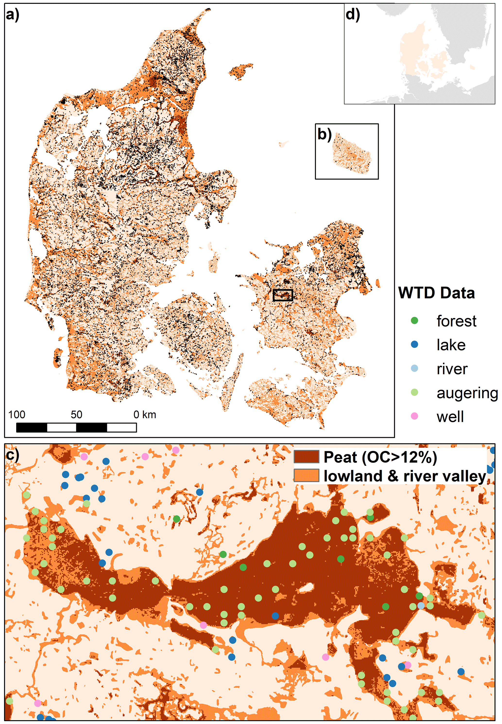
Figure 1 (a) Map of Denmark (b) including the island Bornholm, indicating the entire domain of the WTD model (lowland and river valley) and the focus area with organic content (OC) > 12 %. (c) A zoomed-in view of Åmosen with different sources of WTD data. The WTD data sources are not differentiated in (a) and are simply shown as black dots. Location of (c) is shown in (a) with a black box. (d) Overview of the area indicating the location of Denmark in northern Europe.

2 Data and methods

2.1 Study area

The study area covers the entire land area of Denmark, which corresponds to approx. 43 000 km². In order to restrict the domain for the data analysis and modeling to an area where WTD-driven GHG upscaling may be of relevance, we calculated the union of two map layers that include a river valley bottom delineation (Sechu et al., 2021) and a map of wetlands (Greve et al., 2014). The two map layers correspond to approx. 775 000 ha and approx. 904 000 ha, respectively, and their union, which marks our model domain, amounts to approx. 1 162 000 ha, roughly one-fourth of the total land area of Denmark (Fig. 1). For the final analysis, the domain was further constrained to the carbon-rich lowland soils. The total area of peat soils with organic content (OC) greater than 12 % constitutes approx. 129 000 ha, of which approx. 74 000 are cultivated, either extensively as permanent grassland (35 %) or intensively for a variety of crop types (65 %) (Greve et al., 2019; Levin, 2019). Peat extraction is still taking place sporadically in Denmark. The Danish climate is characterized as temperate with evenly distributed precipitation over the year. The Danish Meteorological Institute states the mean annual temperature as 8.7 ^∘C and the mean annual precipitation as 759 mm.

2.2 Water table depth

A total of 24 492 WTD observations were assembled from various sources in order to compile a comprehensive training dataset that reflects long-term average summer conditions. WTD observations recorded between the months of May and September in the period of 2000 to 2021 were used as training data. Figure 1 depicts the locations of the WTD observations, and Table 1 provides an overview of the different sources and WTD statistics. Data from the Danish well database JUPITER (Hansen and Pjetursson, 2011) were processed by first constraining the well location to a 200 m buffer around the lowland soils. Second, only wells with a maximum filter depth of 5 m below ground were selected. The median WTD was used in cases where a well had multiple observations within the specified period. This resulted in 5716 WTD observations. The wells are primarily located in the fringe areas and only 132 wells coincide with the OC > 12 % class. Moreover, 4796 WTD observations were obtained from two soil auger campaigns (2010 and 2021) that specifically targeted lowland soils with high organic content (Greve et al., 2014). A total of 653 out of the 4796 locations sampled in summer 2010 were revisited in summer 2021, and for the double-sampled locations, the mean WTD was used in the final training dataset. The mean and not the median WTD was calculated for the resampled auger sites because only two measurements were available. The soil auguring equipment was limited to a maximum depth of 1.21 m, and in cases where the water table was not detected by the auger, information could only be derived for the minimum WTD at the given location. In general, the auger and well observations are in fair agreement with each other and show an average deviation of 0.1 m for sampling locations with a difference of less than 100 m. Further, 9980 groundwater-dependent lakes with a surface area greater than 100 m² and located within a 200 m buffer around the peatland soils were used as proxy WTD observations. Since lake water level observations were missing, values were drawn from a normal distribution with an assumed mean of −0.25 m, i.e., above terrain, and a standard deviation of 0.05 m. Additional dummy points for saturated conditions were placed along the coastline and the river network. Here, 1000 points for each category were placed randomly and assigned a WTD of 0 m. Lastly, dummy points for drained conditions were generated along drain ditches and within drained forest. Here, 1000 points for each category were placed randomly and sampled from a normal distribution with a mean WTD of 1.21 m and standard deviation of 0.2 m. Under Danish conditions, ditches drain the agricultural land year-round in most cases. Figure 2 depicts the WTD variability of the training dataset differentiated for the data sources. The WTD data derived from the national well database were the only source that contained deep WTD observations. The data originating from the soil coring campaigns provided mostly shallow data; however, 3110 samples had a WTD of 1.21 m and thereby solely indicated a minimum WTD. The WTD of lakes is entirely above terrain, i.e., negative WTD values, whereas coast and rivers were assigned a WTD of 0 m. We created a training dataset for summer conditions because the WTD observations from the soil auger campaigns are primarily from summer months and the WTD data from this source represent the primary information on the shallow WTD, i.e., the top meter below terrain. Based on the WTD observations from the national well database, the median WTD for summer is 2.0 m, whereas the median WTD for winter is 1.75 m based on the same processing as was applied for the summer data but for the months from October to March. The difference of 0.25 m can be understood as an overall annual amplitude.

Table 1 WTD observations used as training data with information on number of data (n), WTD mean and standard deviation (SD). Sources marked with an asterisk represent dummy points.

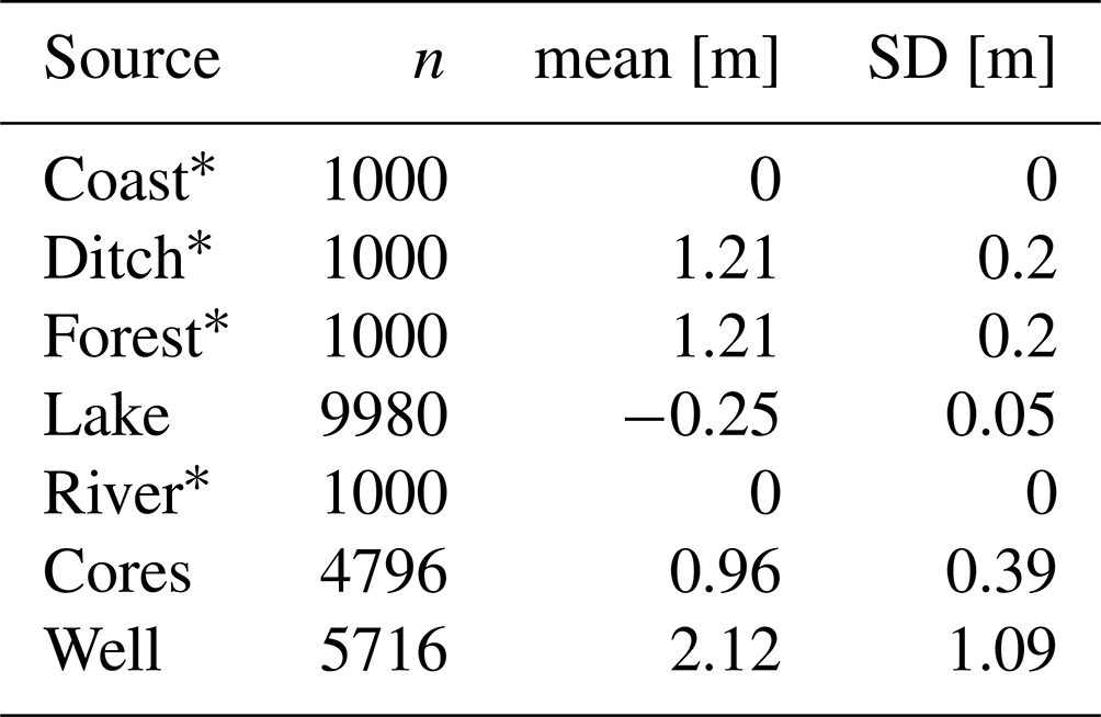
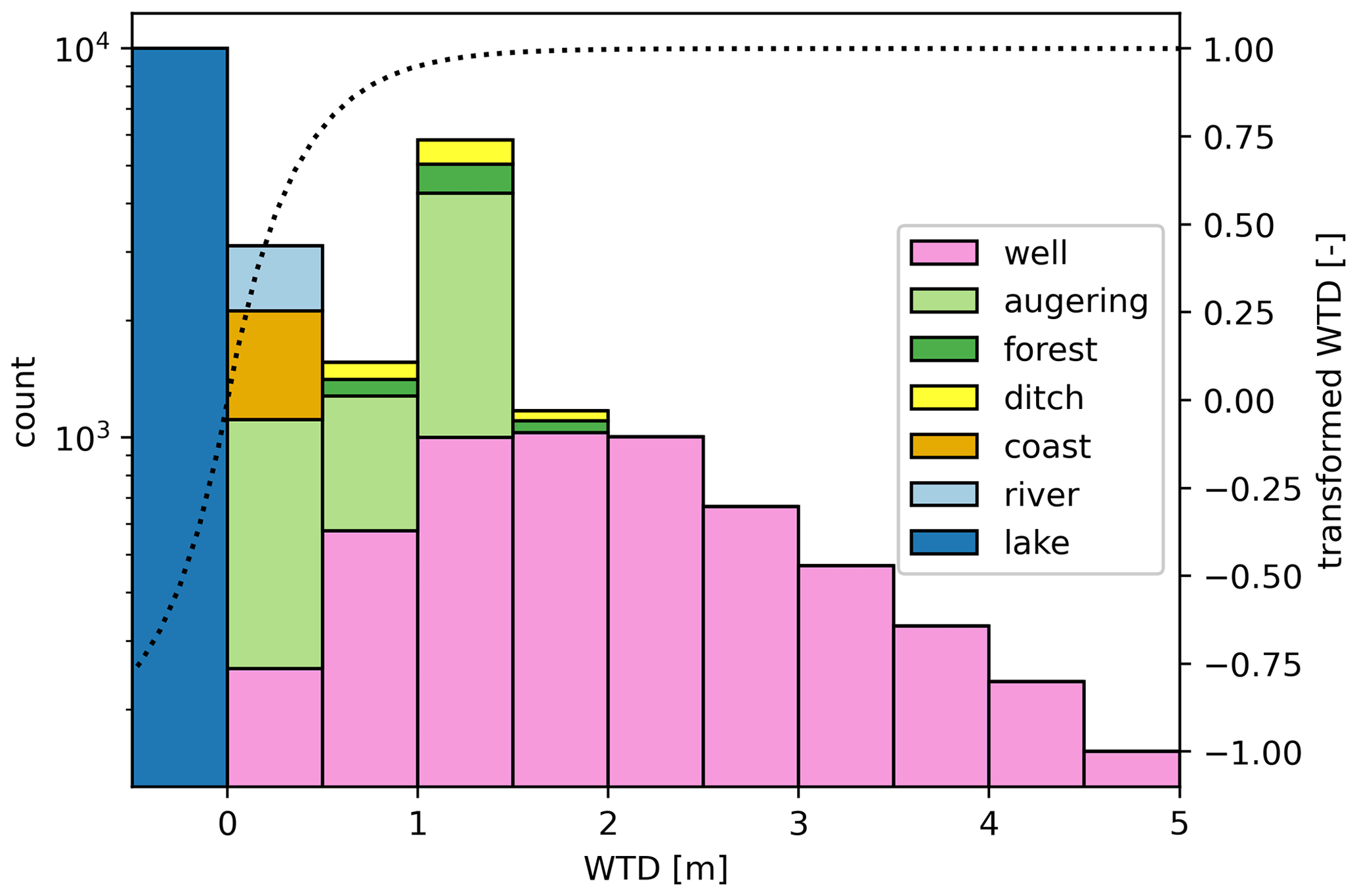
Figure 2 Variability and frequency of the analyzed WTD data with respect to their sources. The dotted line indicates the transfer function yielding transformed WTD (WTD_t) on the secondary y axis.

Based on a data synthesis by Tiemeyer et al. (2020), the WTD-driven GHG response functions of CO₂ and CH₄ emissions from organic soils exhibit a nonlinear relationship with the most distinct sensitivity in the depth interval of 0 to 0.5 m. In consequence, we aim at modeling WTD with the highest possible accuracy for this GHG-sensitive WTD interval. With the same motivation, Bechtold et al. (2014) presented a WTD transformation function that resulted in a pseudo-linearity between WTD and GHG. For our purpose, the transformation function presented by Bechtold et al. (2014) was adapted to

$$\begin{array}{}\text{(1)}& {\mathrm{WTD}}_{\mathrm{t}}=\left\{\begin{array}{ll}{e}^{\mathrm{3}\cdot \mathrm{WTD}}-\mathrm{1}& \mathrm{WTD}<\mathrm{0}\\ \mathrm{1}-e^{-\mathrm{3}\cdot \mathrm{WTD}}& \mathrm{WTD}\ge \mathrm{0}\end{array}\right.,\end{array}$$

where WTD_t is the transformed WTD. As shown in Fig. 2, WTD_t varies between −1 and 1 and reaches its upper asymptote at a WTD of approximately 1 m. The applied WTD transformation also allows us to incorporate the 1.21 m WTD data that represent a minimum observation since the WTD_t variability above 1 m is minimal.

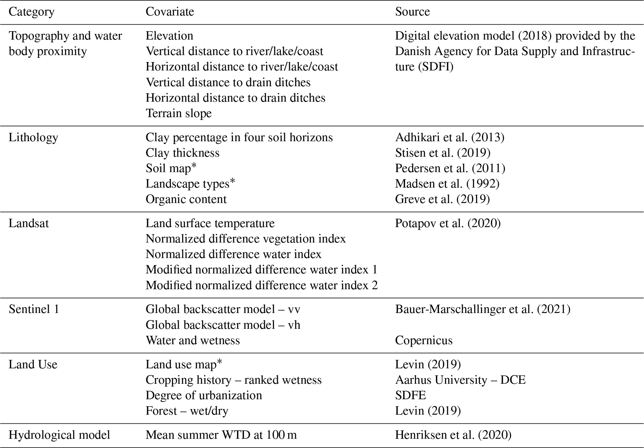
Table 2 Covariates used in the WTD model. Covariates marked with an asterisk are categorical.

2.3 Covariates

A set of 27 covariates was curated to gather national-scale map layers that are deemed relevant to explain the WTD variability in the training dataset (Table 2). The individual maps were resampled from their native resolutions to the defined output resolution of 10 m. The covariates encompassed high-resolution data on topography, water body proximity, lithology, land use and hydrology. The water body proximity was expressed as both the vertical and horizontal distance to the nearest water body, which contained rivers, lakes and the coastline. Additionally, the vertical and horizontal distance to the nearest ditch was calculated to capture the effect of drainage on WTD in lowland soils. Using the historical crop type records, a six-class ranked map indicating wetness of agricultural fields was created. The wetness rank represents a qualitative analysis based on agricultural expert judgment based on the Danish Agricultural Land Parcel Information System for approx. 600 000 fields for the years 2016 to 2020. Moreover, high-resolution data relevant to discriminate saturation conditions of the soil were obtained from Landsat and Sentinel-1 satellite systems, such as land surface temperature (LST), which serves as a valuable proxy for water-saturated soil conditions.

2.4 Machine learning model

We applied the CatBoost implementation of the well-established gradient-boosting decision tree (GBDT) algorithm (Dorogush et al., 2018; Prokhorenkova et al., 2018). In an additive training process, GBDT builds a prediction model based on an ensemble of weak learners, i.e., decision trees. For a pre-defined number of iterations, GBDT attempts to correct itself by adding a decision tree trained against the residuals of the ensemble sum of its predecessors. CatBoost is favorable over similar ML algorithms, such as random forest algorithms, support vector machines, or other GBDT implementations (e.g., XGboost or LightGBM), with respect to computational time and memory usage, while achieving a competitive accuracy (Hancock and Khoshgoftaar, 2020; Huang et al., 2019). The model is set up to predict WTD at a resolution of 10 m. Given the areal extent of the domain, over 116 million grid cells are simulated by the GBDT model. The cost function used in training the model was set to the root-mean-square error (RMSE) and key hyper parameters were tuned via a randomized search. The following CatBoost hyper parameters were included in a simple randomized search with 2000 iterations: learning_rate, depth, subsample, rsm (random subspace method), l2_leaf_reg, min_data_in_leaf. The selected hyper parameters affect the overall architecture of individual trees and limit the effect of overfitting. The best performing model with respect to a 25 % holdout validation was selected for subsequent final training. The final GBDT model was trained over 1000 iterations where 10 % of the data were used as validation data to initiate early stopping once the validation cost function did not improve over 10 iterations. CatBoost allows for assigning weights to the individual training data, which are used to calculate the cost function. In order to emphasize the GHG-sensitive depth interval 0 to 0.5 m in the model training, a weight of 2 was assigned to shallow WTD observations.

The Shapley additive explanations (SHAP) approach (Lundberg and Lee, 2017) was implemented to investigate the covariate importance of the trained GBDT model. SHAP builds upon game theory principles to explain the output of any ML model by quantifying marginal contributions of the applied covariates. SHAP values represent the contribution of each covariate to the final prediction and thereby provide valuable insights into trained ML models. The magnitude and sign of the SHAP values indicate the importance of a covariate and the direction of impact on the prediction, respectively. We calculated SHAP values (i) for the training dataset to get insights into the trained GBDT model and (ii) for the prediction dataset to generate maps showing the relationships between covariates and WTD.

2.5 Synthesis and upscaling of Danish GHG flux data

The first measurements of CO₂ fluxes from cultivated peat soils in Denmark were performed in the 1970s using an in situ alkaline CO₂ trap method (Petersen et al., 1976), but it was not until 2008–2009 that a national monitoring campaign was accomplished, where net fluxes of CO₂, CH₄ and N₂O were measured at eight sites using closed chamber techniques (Elsgaard et al., 2012; Petersen et al., 2012). Data on net ecosystem carbon balance from this campaign (Elsgaard et al., 2012) are used as the current Tier 2 emission factors (EFs) for organic soils with > 12 % OC in Denmark's National GHG Inventory report submitted under the United Nations Framework Convention on Climate Change and the Kyoto Protocol (Nielsen et al., 2021). National campaigns have not been repeated, but a number of research projects have generated additional data on annual emissions of GHGs from Danish organic soils. A synthesis of these studies was performed in the present study (Tables S1 and S2 in the Supplement), and the data were used to derive response functions for GHG emissions in relation to WTD at mean annual conditions.

For analyzing CO₂ emissions, we employed a nonlinear Gompertz function according to Tiemeyer et al. (2020):

$$\begin{array}{}\text{(2)}& {\mathrm{CO}}_{\mathrm{2}}-\mathrm{C}\left(\mathrm{WTD}\right)={\mathrm{CO}}_{\mathrm{2}}-{\mathrm{C}}_{\min }+{\mathrm{CO}}_{\mathrm{2}}-{\mathrm{C}}_{\mathrm{diff}}\cdot e^{-a\cdot e^{b\cdot \mathrm{WTD}}},\end{array}$$

where CO₂−C_min is the lower asymptote, CO₂−C_diff is the difference between upper and lower asymptote, a controls the displacement along the WTD axis and b defines the gradient. Indirect CO₂ emissions from leaching of dissolved organic carbon (CO₂−C_DOC) were added to Eq. (2) based on standard EFs of 0.31 Mg C ha⁻¹ for drained soils and 0.24 Mg C ha⁻¹ for rewetted soils (IPCC, 2014).

For analyzing CH₄ emissions, we fitted an exponential WTD response function according to Tiemeyer et al. (2020) and Evans et al. (2021):

$$\begin{array}{}\text{(3)}& {\mathrm{CH}}_{\mathrm{4}}\left(\mathrm{WTD}\right)={\mathrm{CH}}_{\mathrm{4}\min }+c\cdot e^{-d\cdot \mathrm{WTD}},\end{array}$$

where CH_4 min is the lower asymptote while c and d control the shape of the exponential function (Tiemeyer et al., 2020). The Danish sites for which CH₄ emission data were available represented drained and restored cropland and grassland, including sites where the water level at least under experimental conditions was close to surface. Methane emission from ditches (CH_4 ditch) was estimated by considering a fraction of the land, i.e., 10 %, where drainage ditches are located. As opposed to Tiemeyer et al. (2020), who applied a ditch fraction parameter for all grids, we only included grids that are actually containing a ditch. The location of the ditches was derived based on publicly available datasets. Given the applied grid size of 10 m, this corresponds to an averaged drainage ditch dimension of 1 m, which can be considered very suitable for Danish conditions. The applied EFs for CH_4 ditch were 1165 $\mathrm{kg}{\mathrm{CH}}_{\mathrm{4}}{\mathrm{ha}}^{-\mathrm{1}}{\mathrm{yr}}^{-\mathrm{1}}$ for cropland and 948 $\mathrm{kg}{\mathrm{CH}}_{\mathrm{4}}{\mathrm{ha}}^{-\mathrm{1}}{\mathrm{yr}}^{-\mathrm{1}}$ for grassland (IPCC, 2014), where the latter represents the weighted average of IPCC's shallow (34 %) and deep (66 %) drained grassland EFs, as applied in Tiemeyer at al. (2020).

Data for N₂O emissions showed no systematic WTD dependence, and as a consequence land-use-specific EFs were applied. We applied the EFs from Wilson et al. (2016) as updated from the IPCC (2014) wetlands supplement: 13.0 $\mathrm{kg}{\mathrm{N}}_{\mathrm{2}}\mathrm{O}-\mathrm{N}{\mathrm{ha}}^{-\mathrm{1}}{\mathrm{yr}}^{-\mathrm{1}}$ for cropland, 4.7 $\mathrm{kg}{\mathrm{N}}_{\mathrm{2}}\mathrm{O}-\mathrm{N}{\mathrm{ha}}^{-\mathrm{1}}{\mathrm{yr}}^{-\mathrm{1}}$ as average for grassland (deep or shallow drained, nutrient rich or poor) and 0.1 $\mathrm{kg}{\mathrm{N}}_{\mathrm{2}}\mathrm{O}-\mathrm{N}{\mathrm{ha}}^{-\mathrm{1}}{\mathrm{yr}}^{-\mathrm{1}}$ for rewetted organic soils.

All GHGs were converted to CO₂-eq using their global warming potential (GWP) over a 100-year period according to the sixth IPCC assessment report (Forster et al., 2021) where 1 kg CH₄ = 27 kg CO₂ and 1 kg N₂O = 273 kg CO₂. For applying the land-use-specific EFs and WTD response functions, we used a 2020 land use classification for Denmark (Levin and Gyldenkærne, 2022). Based on the available WTD observations, the WTD map captures a long-term average summertime condition. Since the applied GHG upscaling method is based on annual mean WTD, a scaling parameter is subtracted from the summertime WTD map to obtain an annual average. As described in Sect. 2.2, the annual variability is estimated to be 0.25 m. In order to correct for seasonality, 0.125 m was subtracted from the summer WTD map. Negative values were set to zero.

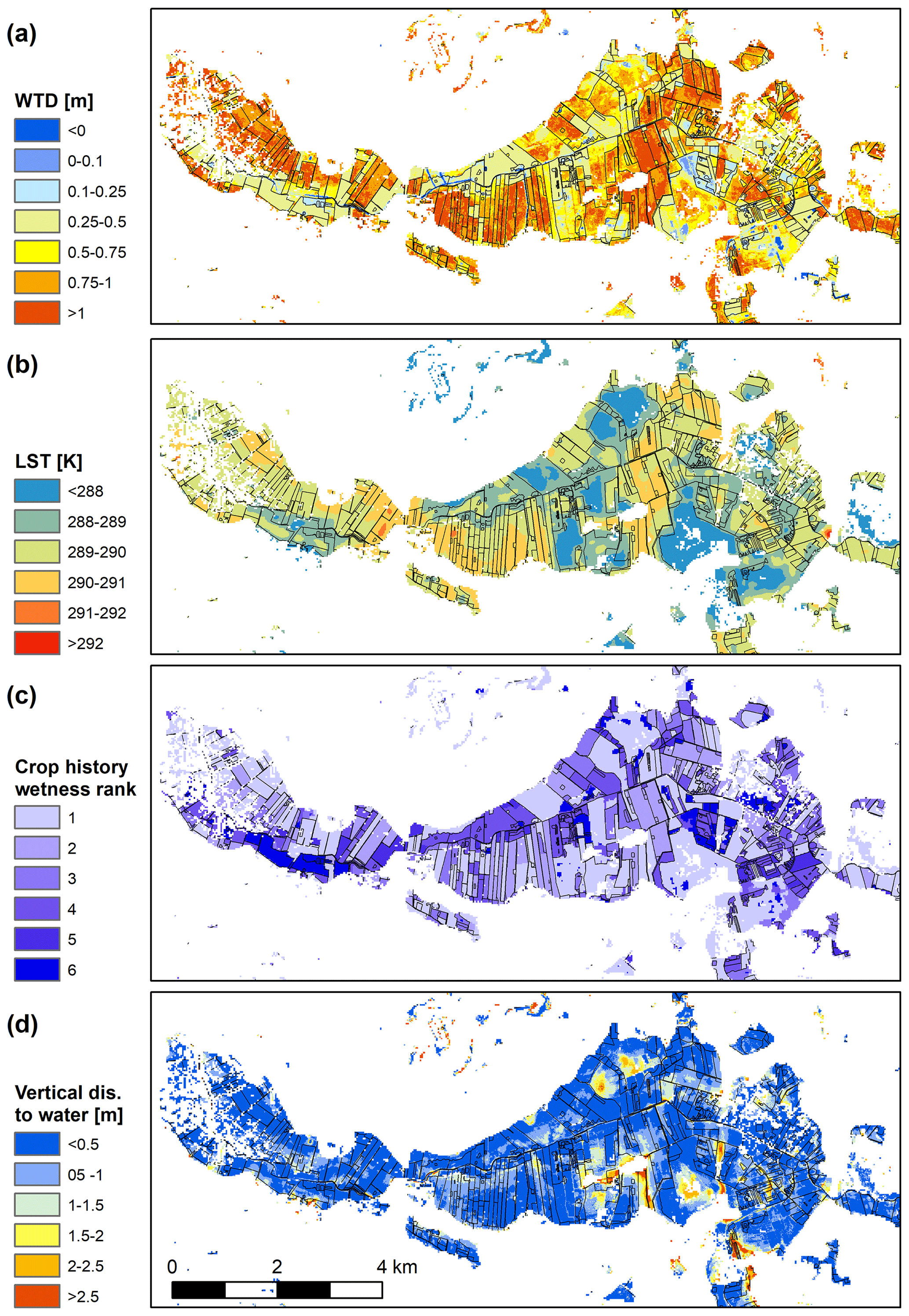
Figure 3 (a) The modeled WTD map at 10 m resolution for Åmosen (the zoomed-in area shown in Fig. 1c). The three key covariates of (b) land surface temperature (LST), (c) wetness rank derived from the 2016 to 2020 cropping history and (d) vertical distance to nearest water body (river, lake or coast) are shown. Polygons showing the delineation of agricultural fields are added to all panels.

3 Results

3.1 Water table depth model

The hyperparameter tuning of the GBDT model resulted in the following results: depth = 10, learning_rate = 0.05, subsample = 0.8, rsm = 0.8, min_data_in_leaf = 1 and l2_leaf_reg = 5. The GBDT model was trained against WTD_t, but throughout the paper results and analyses are based on the back-transformed variable WTD. Figure 3 depicts the final simulated WTD map that represents a long-time average summertime condition for the period of 2000 to 2021 for Åmosen, which is one of the largest peatlands in Denmark. For the visual assessment, a color scheme that emphasizes the depth interval of 0 to 1 m has been selected. Even though WTD is simulated for a larger domain (lowland soils and river valleys), only grid cells with OC > 12 % are shown since the applied GHG upscaling method is only valid for such conditions. The WTD map discloses a distinct spatial heterogeneity with fully saturated conditions laying in very close vicinity to well-drained conditions.

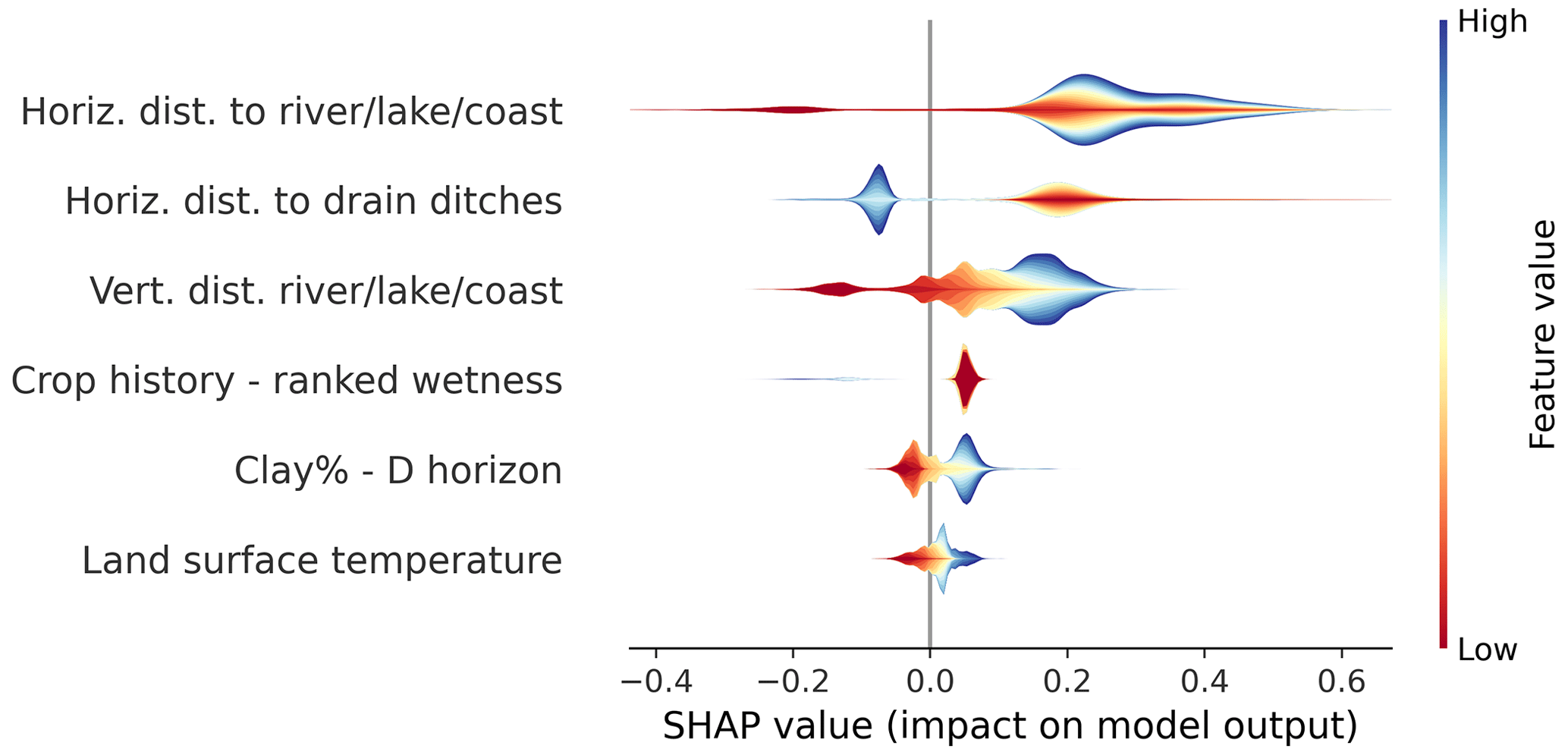
Figure 4 SHAP values for the six most important covariates based on an analysis using all well and auger WTD observations. The SHAP value interprets the covariate's impact on the prediction. The violin plots are color coded based on the stacked values of the covariates, and the height indicates the density of the data.

We applied SHAP to investigate feature importance of the trained GBDT model for the well and auger WTD observations, i.e., excluding the dummy points (Fig. 4). The six most important covariates were, ordered in high to low importance: horizontal distance to water bodies, horizontal distance to ditches, vertical distance to water bodies, wetness rank based on cropping history, clay content of the deepest soil horizon and land surface temperature (LST). Negative SHAP values are associated to negative impact, i.e., more shallow WTD and positive SHAP values are linked to a deeper water table. Locations close to water bodies exclusively possess negative SHAP values whereas locations with a large horizontal distance to the closest water body have both negative and positive SHAP values. The SHAP values for the horizontal distance to drain ditches are separated with positive values (producing a deeper WTD) for low distances, which clearly reveals the functioning of the added dummy points representing well-drained conditions along the drain ditches. The interpretation of the SHAP values for the vertical distance to water bodies is that WTD does not follow small-scale topographical variation and instead the water table has a smoother variation than topography, which results in a deeper WTD (positive SHAP value) for areas with a high vertical distance to the nearest water body. The wetness classes based on the cropping classes show a clear WTD sensitivity, where the low ranks, which are linked to crops that favor well-drained conditions possess positive SHAP values, and the wet classes relate to a negative impact on the simulated WTD. A high clay percentage produces a positive impact on the prediction, i.e., deeper WTD. LST also shows a clear link to WTD, with higher values yielding a deeper WTD and lower LST, resulting in more water-saturated conditions.

Figure 3 exemplifies three of the seven listed covariates (i.e., LST, wetness rank and vertical distance to nearest water body) to elucidate key connections between model input and output. For LST (Fig. 3b), there is a direct relationship, with lower LST in areas of high saturation caused by either evaporative cooling of the land surface due to high water availability or enhanced heat conductance towards deeper layers for wet soils, whereas deeper water tables, i.e., drier conditions, are collocated with higher LST. Further, we observe a good agreement between WTD and the wetness rank, derived from the cropping history from 2016 to 2020 (Fig. 3c). Fields with crops associated with a wet rank, i.e., permanent poor grassland with low nitrogen application rates, are associated with a low WTD, while crops that require drainage, e.g., winter wheat, potatoes or sugar beet, are found at fields with a deeper WTD. The agronomic requirements reflected by the ranked wetness map are characterized by plausible mean WTD, which show consistent differences between each other. For the entire domain, the mean WTD values for the three wettest categories are below 0.4 m, whereas the three dry categories have a WTD of 0.65 m and deeper. LST and wetness rank are to some degree connected to each other, with a lower LST for crops with a higher wetness rank. However, exceptions are found for drained forests that are associated with a low LST and a low wetness rank. Topographical variability is generally low in peatlands. Nevertheless, the vertical distance to the closest waterbody reveals small-scale topographical features that effect the simulated WTD (Fig. 3d).

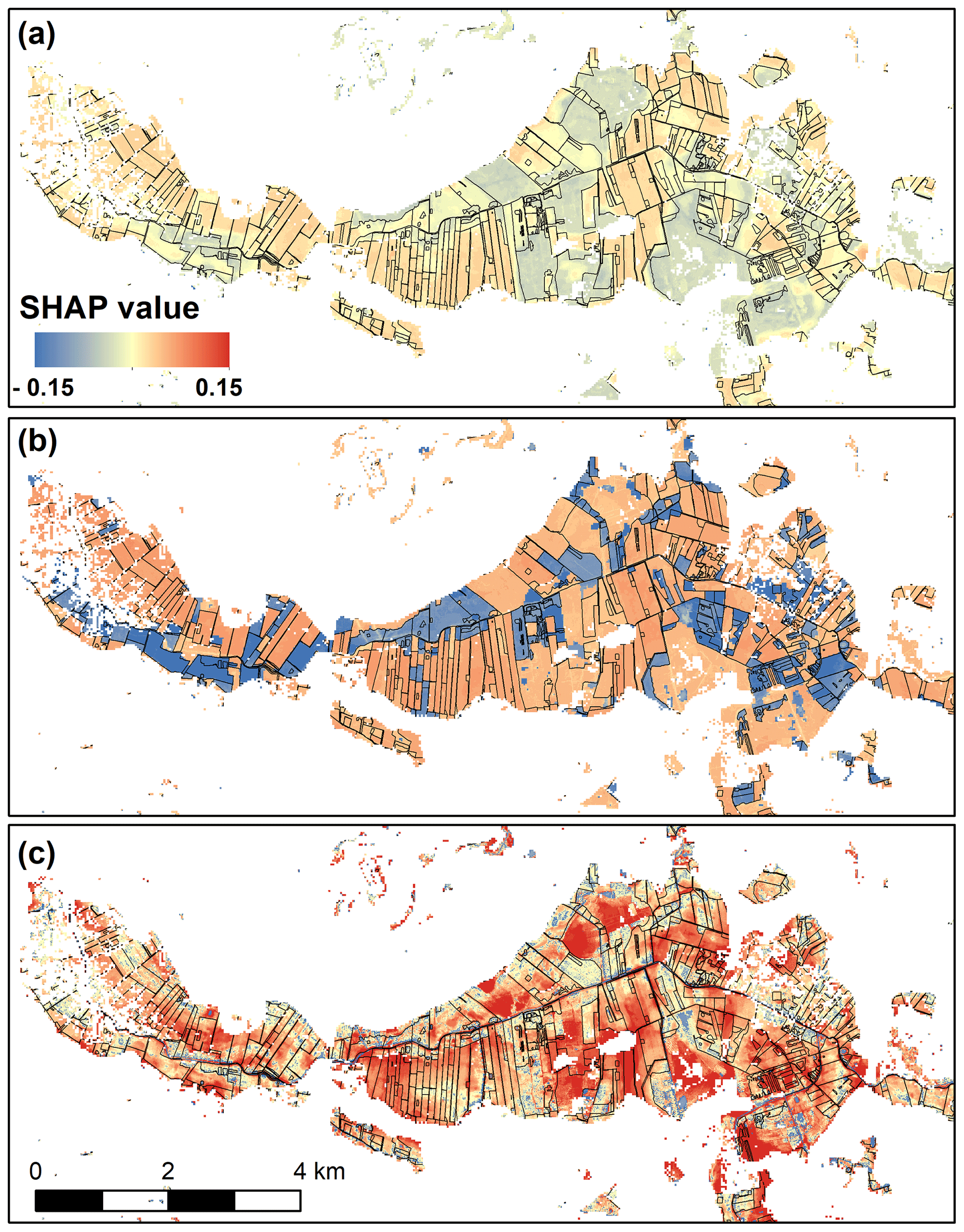
Figure 5 SHAP values for the prediction dataset shown for three selected covariates: (a) LST, (b) wetness rank derived from the 2016 to 2020 cropping history and (c) vertical distance to nearest waterbody. Results are shown for Åmosen (the zoomed-in area shown in Fig. 1c).

Figure 5 depicts the spatial distribution of SHAP values for the same three covariates substantiates previous findings (Fig. 4). High LST has a positive impact on the prediction, resulting in deep WTD, and low LST has a negative impact on the prediction. In the case of drained forest, which has a low LST, the negative impact of LST is overruled by the positive impact of the crop-based wetness rank. The latter shows a very clear separation of negative impact for the wet ranks and positive impact for the dry ranks. The negative impact of the vertical distance to the nearest waterbody is predominately limited to locations that are actually river or lake grids. A distinct positive impact is found for locations with a high vertical distance.

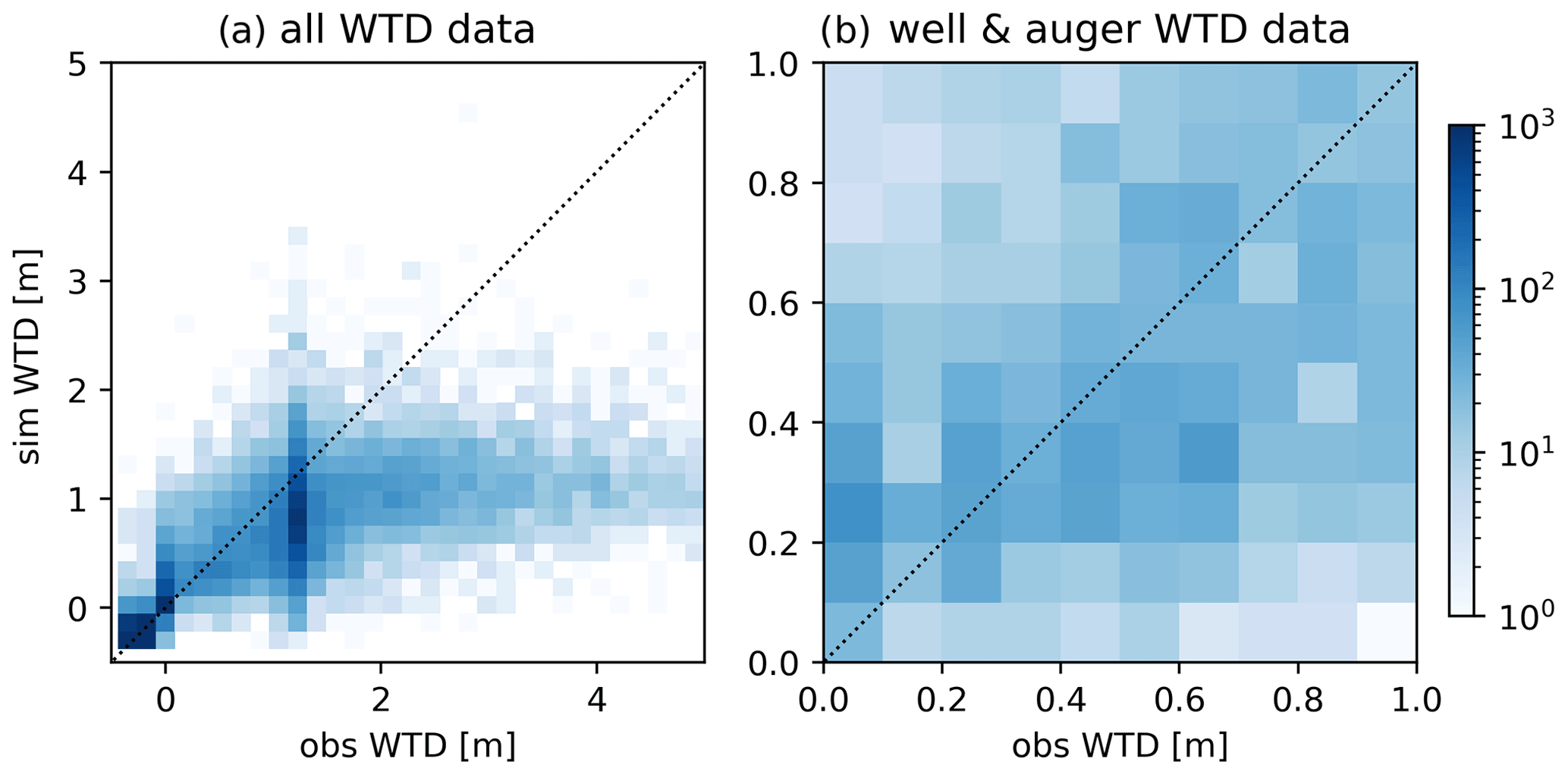
Figure 6 Density scatter plots, with 0.2 m bins, for the applied 5-fold cross-validation test. The dotted line represents the 1:1 line between observed (obs) and simulated (sim) WTD. The color bar indicates the data count for each bin. In (a) all WTD data are plotted, and in (b) only a subset containing the well and auger observation are shown for the WTD interval of 0 to 1 m.

In order to assess the overall accuracy of the WTD map, we conducted a 5-fold cross-validation experiment. For this, five GBDT models were trained using 80 % of the data for training, and 20 % of the data were held back for validation. The five validation datasets were sampled so each WTD observation served exactly once as validation data. Figure 6 presents the scatter density plot of both observed and simulated WTD for the five validation datasets, with Fig. 6a including the dummy points and Fig. 6b excluding them. The effect of the WTD transformation and the weighting scheme of WTD data in the depth interval of 0 to 0.5 m becomes apparent. The model shows the best accuracy for the shallow water table interval, whereas the performance deteriorates below a WTD of 1 m. The poor performance of WTD below 1 m can be explained by the transfer function which hinders the GBDT model to discriminate WTD variability below a WTD of 1 m. In the case of WTD-driven GHG upscaling, this is acceptable since the applied WTD response functions are not sensitive to changes in WTD deeper than approx. 0.5 m. The scatter plot reveals that the dummy points with zero and negative WTD, i.e., above terrain, are generally represented quite well by the GBDT model. Taking only the well and auger WTD observations into consideration, a slight bias for the shallow WTD observations becomes evident.

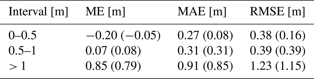
Table 3 quantifies the performance of the GBDT model for the 5-fold cross-validation test both including and excluding the dummy points. The performance for the well and auger observations for the top 0.5 interval shows a bias of −0.2 m. Also taking dummy points into consideration, the bias of the top 0.5 m interval and the 0.5 to 1 m interval was −0.05 and 0.08 m, respectively. We consider the validation excluding the dummy points as the more relevant performance quantification for the given application. For the deeper intervals the metric scores are comparable for the entire training dataset and the subset exclusively based on well and auger data. WTD values deeper than 1 m perform worst of all stated metrics, which underpins the visual assessment of Fig. 6.

Table 3 Performance of the 5-fold cross-validation test for three depth intervals assessed by three metrics: mean error (ME), mean absolute error (MAE) and root-mean-square error (RMSE). Only well and auger WTD observations were considered for the evaluation. The metric scores for all data, i.e., including the dummy points, are stated in parentheses.

For the entire model domain, the GBDT model predicts a WTD interval sensitive to GHG variability, i.e., 0–0.5 m, for 36 % of the area. For the delineated peat soils, with OC > 12 %, this area amounts to 54 %. After correcting from summer to annual conditions, i.e., subtracting 0.125 m (half the mean annual amplitude), these area estimates increase to 45 % and 64 %, respectively. For agricultural areas with OC > 12 %, the mean WTD is 0.49 m with a standard deviation of 0.35 m, which underpins the distinct WTD variability in peatlands, and this is also partly overlapping with the range of WTD associated with high sensitivity of the resulting emissions of CO₂, CH₄ and N₂O.

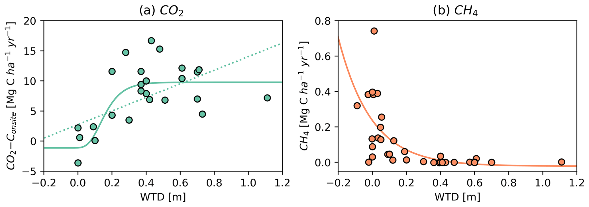
Figure 7 Annual net ecosystem carbon balance of CO₂ (a) and emissions of CH₄ (b) in Danish organic soils plotted against mean water table depth (WTD). For CO₂, a Gompertz model (solid line) and a linear model (dotted line) have been fitted. For CH₄ an exponential model has been fitted. Sources of data are shown in Supplementary Table S1.

3.2 Danish greenhouse gas response functions

The parametrization of the fitted WTD-driven response functions for CO₂ and CH₄ emissions (Fig. 7) showed a systematic relationship where CO₂ emissions increased with increasing WTD between 0 and 0.4–0.5 m before reaching an asymptotic level of 10 $\mathrm{Mg}{\mathrm{CO}}_{\mathrm{2}}-\mathrm{C}{\mathrm{ha}}^{-\mathrm{1}}{\mathrm{yr}}^{-\mathrm{1}}$. The fitted parameters are as follows: CO₂−C_min = 1.132 Mg CO₂-C ha¹⁻ yr⁻¹, CO₂−C_diff = 10.903 Mg CO₂-C ha¹⁻ yr⁻¹, a = 6.415 and b = 14.183 m⁻¹. CH₄ emissions were consistently negligible at WTD depths below 0.2–0.3 m, but they increased at higher WTD to emissions of up to 0.8 $\mathrm{Mg}\mathrm{C}{\mathrm{ha}}^{-\mathrm{1}}{\mathrm{yr}}^{-\mathrm{1}}$. However, it is clear that a shallow WTD does not necessarily cause high CH₄ emissions, but it instead provides a window of opportunity for methane fluxes to the atmosphere. The fitted parameters are as follows: CH_4 min = −21.48 kg C ha⁻¹ yr⁻¹, c = 258.83 and d = −5.16 m⁻¹. N₂O emissions were not modeled, but average values for observations at WTD > 0.3 m (n = 19) and < 0.3 m (n = 6) were 13.3 and 3.8 $\mathrm{kg}\mathrm{N}{\mathrm{ha}}^{-\mathrm{1}}{\mathrm{yr}}^{-\mathrm{1}}$, respectively, thus representing a value similar to IPCC EFs for drained soil but a value somewhat higher for rewetted soils (Wilson et al., 2016).

3.3 Upscaled greenhouse gas emissions

Upscaling GHG emissions can be estimated based on the following elements: (1) the GHG upscaling method presented in Sect. 2.5, (2) the long-term annual average WTD map, (3) a land use map and (4) a map delineating the drainage ditches. With a spatial resolution of 10 m, the WTD maps open the possibility to estimate GHG at equally high resolution. However, given the apparent uncertainties in the WTD map and the WTD response functions, GHG values are aggregated to national scale.

For the approximately 74 000 ha with OC > 12 %, the total emission of the three gases CO₂, N₂O and CH₄ amounts to 2.6 Mt CO₂-eq. Figure 8 depicts the relationship between WTD and the estimated GHG emissions, expressed as emission factor converted to CO₂-eq. Emissions of CO₂ dominate the GHG budget at WTD deeper than approx. 0.1 m, whereas methane emissions become dominant at WTD closer to the soil surface. The contribution from CH₄ emissions is apparent, starting from a WTD of approx. 0.3 m, whereas low CH₄ emissions for deeper WTD are related to the minor CH_4 ditch component, which is not WTD dependent and takes place throughout the lowland soils. N₂O emissions have no WTD response function, and thus emissions are rather constant across the WTD variability. Spatial heterogeneity of N₂O emissions is based on the applied land-use-specific emissions factors that are indirectly linked to WTD variability, which results in a slight decrease in N₂O emissions with decreasing WTD. Based on the minimum of total GHG emissions shown in Fig. 8, a WTD of approx. 0.04 m can be identified as the optimal WTD for minimal GHG emissions, i.e., 5.6 Mg ${\mathrm{CO}}_{\mathrm{2}}\text{-}\mathrm{eq}{\mathrm{ha}}^{-\mathrm{1}}{\mathrm{yr}}^{-\mathrm{1}}$. Yet, the exact numbers should be viewed as indicative, since for example the possibility of negative CO₂ emissions at low WTD depends on the presence of wetland vegetation. Nevertheless, even in the absence of negative CO₂ emissions, the data indicates that an optimal rewetting strategy should aim for a WTD in a range between 0 and 0.1 m to balance the trade-off between CO₂ and CH₄ emissions.

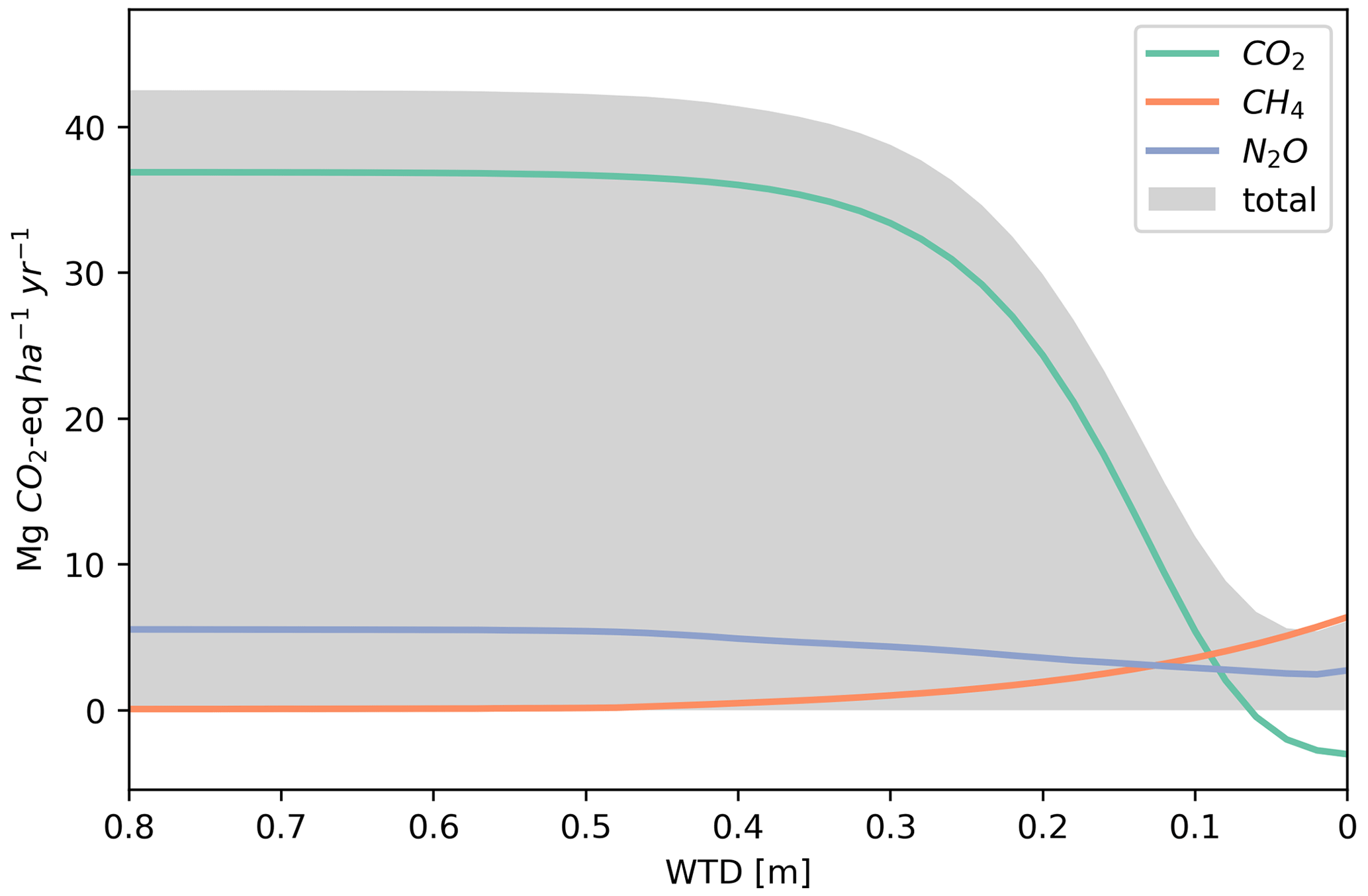
Figure 8 The relationship between greenhouse gas emissions (CO₂, CH₄ and N₂O) and WTD. The emissions are stated in CO₂ equivalents by applying 100-year global warming potentials: 1 kg CH₄ = 27 kg CO₂ and 1 kg N₂O = 273 kg CO₂.

Table 4 The implied emission factors for organic soils with OC > 12 % for CO₂−C_organic, CH_4 organic, N₂O−N_organic and for the sum of greenhouse gas (GHG) emissions applying 100-year global warming potentials: 1 kg CH₄ = 27 kg CO₂ and 1 kg N₂O = 273 kg CO₂. The applied land use map is derived from Levin and Gyldenkærne (2022).

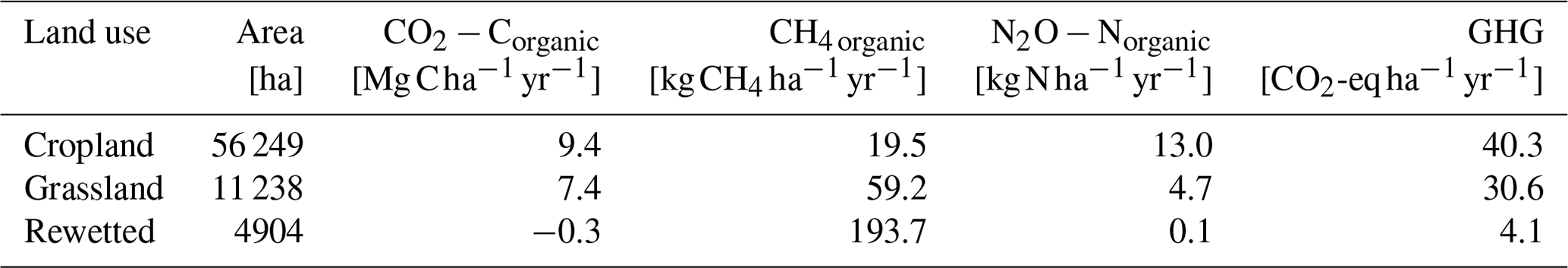
Table 4 states the emission factors for the three considered land use classes. The emission factors for N₂O are in direct agreement with the ones stated in Sect. 2.5, whereas the emission factors for CO₂ and CH₄ are affected by the modeled WTD variability. In total, based on both area and emission factor, cropland dominates the GHG emissions of peatlands in Denmark. As expected, emission factors from rewetted peat soils are lowest.

3.4 Rewetting scenarios

The combination of a high-resolution WTD map and WTD response functions of GHG emissions allows us to evaluate the effects of alternative rewetting scenarios. For this, it is assumed that the WTD of an agricultural field can be changed to the optimal WTD, allowing a reduction in total GHG emissions to 5.6 Mg ${\mathrm{CO}}_{\mathrm{2}}\text{-}\mathrm{eq}{\mathrm{ha}}^{-\mathrm{1}}{\mathrm{yr}}^{-\mathrm{1}}$ (Fig. 8). Figure 9 shows the results of three rewetting scenarios and a theoretical baseline as functions of the peatland area that is rewetted with a maximum of 74 000 ha. The baseline expresses the theoretical maximum emission reduction with the assumption that all agricultural fields are originally well drained and thus having a uniform reduction of 36.8 Mg ${\mathrm{CO}}_{\mathrm{2}}\text{-}\mathrm{eq}{\mathrm{ha}}^{-\mathrm{1}}{\mathrm{yr}}^{-\mathrm{1}}$, which expresses the reduction from the maximum asymptote to the minimum of the total GHG curve in Fig. 8. In the three rewetting scenarios, the reference emissions are derived from the WTD response functions, and thus many agricultural fields have a lower reference emission than the baseline, which will result in a decreased emission reduction with respect to the baseline. The first scenario prioritizes wet fields in the restoration; i.e., the agricultural fields with the most shallow mean WTD are prioritized in the rewetting strategy. This scenario can be regarded as pessimistic with respect to the expected GHG emission reduction. The second scenario prioritizes the dry fields with the deepest mean WTD, which in turn can be considered an optimistic scenario. The third scenario selects fields in a random order and lies in between the optimistic and the pessimistic scenarios. The prioritization order is based on over 79 000 digitized fields, and the WTD of an entire field is set to 0.04 m for calculating the reduction in GHG emissions. In cases where the entire peatland area is rewetted, the reduction in GHG emissions is estimated to be 2.0 Mt CO₂-eq yr⁻¹ by all three scenarios. However, we observe large discrepancies between the restoration scenarios if only a fraction of the total peat area is rewetted. Prioritizing dryer fields already provides a high reduction starting with the first rewetted fields, whereas prioritizing wet fields shows little reduction. In fact, the reduction potential in the wet scenarios is just 30 % of the dry scenario for the first 10 000 ha. A deviation of 50 % between wet and dry scenarios is first exceeded for a rewetting area of above 20 000 ha. The random scenario lies in between the optimistic and pessimistic scenarios, with a linear emission reduction of 26.1 $\mathrm{Mg}{\mathrm{CO}}_{\mathrm{2}}\text{-}\mathrm{eq}{\mathrm{ha}}^{-\mathrm{1}}{\mathrm{yr}}^{-\mathrm{1}}$. The linear emission reduction of the random scenario is 10.7 $\mathrm{Mg}{\mathrm{CO}}_{\mathrm{2}}\text{-}\mathrm{eq}{\mathrm{ha}}^{-\mathrm{1}}{\mathrm{yr}}^{-\mathrm{1}}$ lower than the baseline scenario. This relates to the WTD map that introduces spatial variability in the random scenario opposed to the fully drained conditions assumed in the baseline scenario.

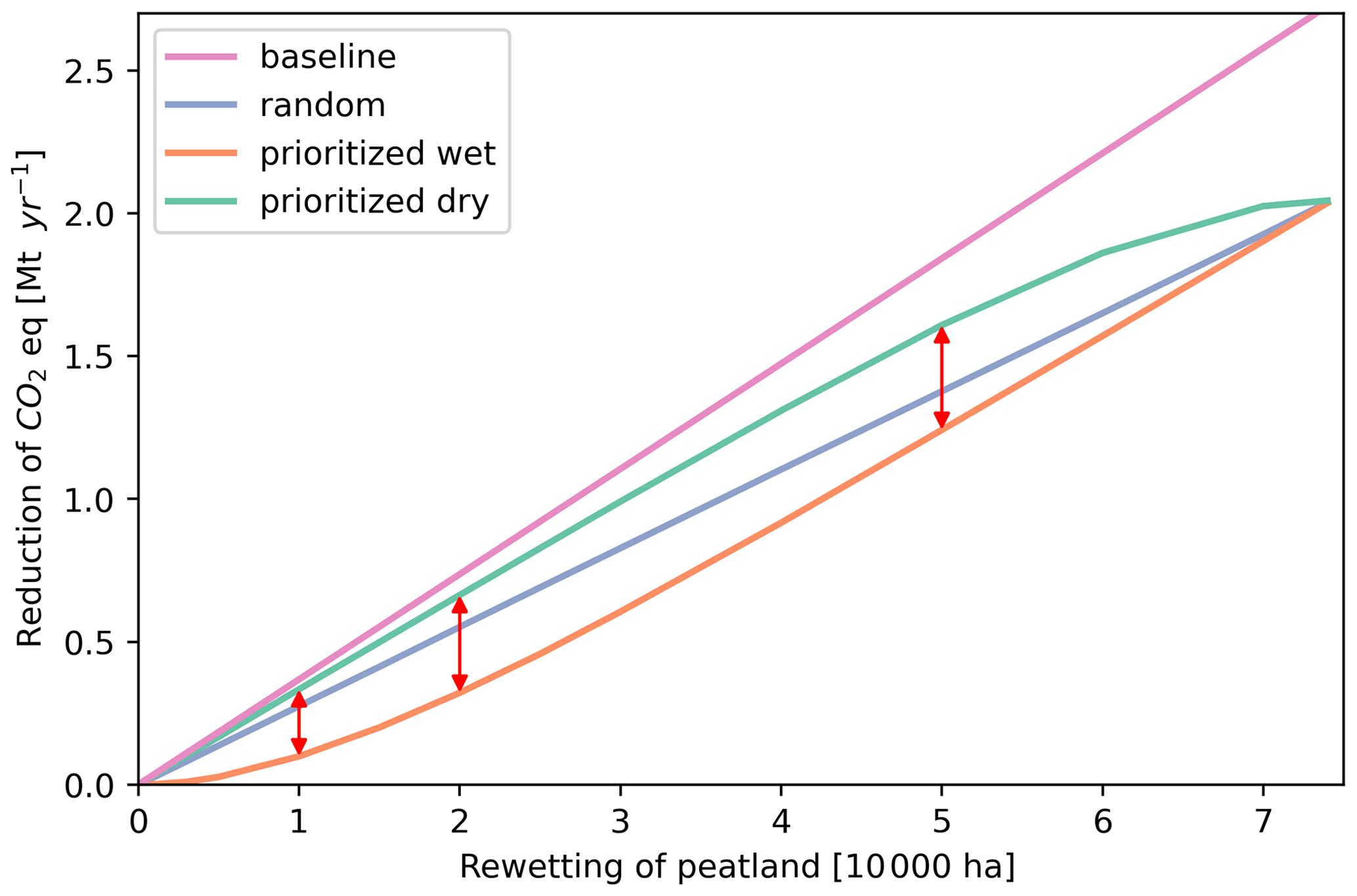
Figure 9 The estimated reduction in GHG emissions in CO₂ equivalents as a function of the area of rewetted peatland. Four scenarios are tested to investigate the potential mitigation effect of alternative rewetting strategies. The red arrows visualize the differences between the wet and dry prioritization scenarios.

4 Discussion and conclusion

Machine learning can utilize the broad spectrum of geo-environmental big data to model WTD on a national scale in Denmark with a reasonable accuracy, taking the quality of available WTD observations into consideration. The 5-fold cross-validation experiment revealed an acceptable residual variance for the most shallow WTD interval (MAE of 0.08 m). Despite all efforts to fine-tune the GBDT model to perform well for the shallow WTD interval, a considerable residual variance (MAE of  0.27 m) was evident when only taking the well and auger WTD observations into consideration. As a consequence of the applied WTD transformation, performance decreased substantially for the deeper WTD. Similar findings were documented by Bechtold et al. (2014), which are mainly related to the applied WTD transformation. However, several sources of uncertainties remain to be addressed, such as the difficulties in modeling a long-term average WTD based on a heterogenous training dataset containing observations from summer months from different years. The training dataset has been curated to represent a steady-state model despite evident WTD fluctuations in peatlands that quickly respond to precipitation events. Future work should aim to reduce uncertainties homogenizing WTD observations, e.g., by normalizing to climate variability to derive a more representative training dataset. Moreover, WTD observations from several sources are used for curating the training dataset. We find a fair agreement between the auger and well WTD observations with a deviation of 0.1 m for sampling points in close vicinity of each other. Despite the above-mentioned challenges and uncertainties, we believe that the comprehensive training dataset provides meaningful information to the GBDT model to predict an average summertime condition.

The SHAP analysis revealed that topography, water body proximity and land use were the most important covariates in the trained GBDT model. Similar findings were reported by other WTD ML-based modeling studies (Bechtold et al., 2014; Koch et al., 2019). The sign and magnitude of the SHAP values provided detailed knowledge on how covariates are linked to WTD. Similar findings have been obtained by Bechtold et al. (2014) applying partial dependence plots. In contrast to Koch et al. (2019, 2020), who modeled WTD over the entire land area of Denmark, we found geology-related covariates less informative for modeling exclusively peat-based soils. It remains unresolved if this relates to the poorer quality of lithological and geological information in peatlands or if peatland hydrology processes are predominately controlled by topography and waterbody proximity.

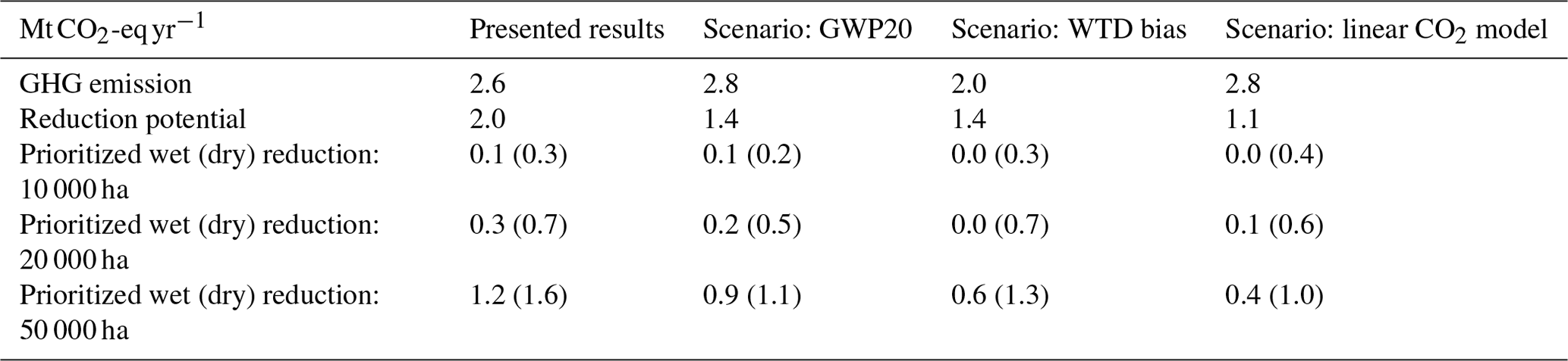
Table 5 Overview of the estimated GHG emissions and reduction potentials (Mt CO₂-eq yr⁻¹) for the wet and dry prioritization scenarios. The sensitivity of the presented results with respect to the applied global warming potential (GWP), WTD bias and the applied WTD response function for CO₂ is assessed.

The Gompertz parametrization of the WTD response function for CO₂ for Danish organic soils (Fig. 7) was strikingly similar to a parametrization based on a larger German dataset (Tiemeyer et al., 2020). Hence, applying the parameters from Tiemeyer et al. (2020) in our upscaling study resulted in CO₂ emissions that deviated by just 1 % on average with respect to the CO₂ emissions based on the Danish Gompertz parametrization. This underlines the strong and consistent effect of WTD as a driver of CO₂ emissions from organic soils across climatic and agroecological conditions. Similar conclusions were reached when comparing our parametrization of the CH₄ response function with the German parametrization (Tiemeyer et al., 2020).

However, although supported by the present study and Tiemeyer et al. (2020). the asymptotic WTD response curve for CO₂ emissions may not be universally applicable. Evans et al. (2021) analyzed CO₂ emissions based on published eddy covariance studies of boreal and temperate peatlands and suggested a linearly increasing emission with increasing WTD. The Danish CO₂ data presented here are predominately in the linear range of the Gompertz function (0–0.5 m). In Fig. 7 we present a linear model fitted to the Danish CO₂ data and contrast it to the applied Gompertz function. The fitted model possesses a slope of 11.29 $\mathrm{Mg}{\mathrm{CO}}_{\mathrm{2}}\text{-}\mathrm{eq}{\mathrm{ha}}^{-\mathrm{1}}{\mathrm{yr}}^{-\mathrm{1}}{\mathrm{m}}^{-\mathrm{1}}$ and an intercept of 2.75 $\mathrm{Mg}{\mathrm{CO}}_{\mathrm{2}}\text{-}\mathrm{eq}{\mathrm{ha}}^{-\mathrm{1}}{\mathrm{yr}}^{-\mathrm{1}}$. The positive intercept is disputable and is not in line with Evans et al. (2021) and the general assumption that organic carbon accumulates under fully saturated conditions. When assessing the fit between modeled and observed CO₂, we find a favorable correlation coefficient when evaluating the Gompertz model over the linear model. Future research should target measuring GHG emissions at sites with a shallow unsaturated zone in order to be able to make a more profound evaluation of the potential for developing a linear model for the WTD response function of CO₂. Additionally, GHG emissions at thick unsaturated peat soils are required to investigate how a linear response function can be extrapolated to deeper WTD. Nevertheless, if taking the actual peat depth into consideration, which can be considered a lower boundary of the response functions, applying a linear model may provide comparable results in the present analysis. However, a high-quality peat depth map is required to substantiate this statement. Both studies, Evans et al. (2021) and Tiemeyer et al. (2020), provide similar findings for the shape of the CH₄ response function, which can be further substantiated by the Danish flux data.

A sensitivity analysis of the WTD bias has been conducted to underpin the discussion points presented above, and the choice of WTD response model was tested for the same reason. As an additional sensitivity analysis, we also addressed the short-term effects of rewetting strategies by applying a 20-year GWP complementary to the 100-year GWP presented in the main results. The results of the three scenarios are presented in Table 5 and compared to the already presented results. In the GWP20 scenario, we changed the GWP for CH₄ from 27 to 81 kg CO₂ (Forster et al., 2021). The overall annual GHG emission increased to 2.8 Mt CO₂-eq yr⁻¹, and since the CH₄ contribution is highest for shallow WTD, the reduction potential is lower in this scenario.

We found a ME of −0.2 m for the uppermost WTD interval, indicating that the GBDT model simulated a water table that is too deep. In the WTD bias scenario, the WTD map is bias corrected across the entire domain. The resulting WTD map is closer to the surface and results in a lower overall emission estimate of 2.0 Mt CO₂-eq yr⁻¹. The differences between wet and dry rewetting scenarios are large because many areas will have a WTD very close to 0 after bias correction and thereby a reduction potential close to 0. This sensitivity analysis represents a simple bias correction of the WTD map whereas a true improvement of the WTD map would likely require an enhanced WTD training dataset with lower uncertainties.

Applying the linear CO₂ WTD response function, the overall GHG emission estimate increases slightly to 2.8 Mt CO₂-eq yr⁻¹. The very shallow and deep WTD intervals possess an increased CO₂ emission compared to the Gompertz model, whereas the intermediate WTD interval (0.2–0.6 m) has a decreased CO₂ emission, but these changes outweigh each other. The reduction potential is much lower, which has to be interpreted with caution, because of the positive intercept of the linear model. The differences between wet and dry rewetting scenarios are large due to high CO₂ emissions when simply extrapolating the linear WTD relationship to WTD > 1 m.

To synthesize the applied scenario analysis and to provide a quantification of the related uncertainties, we have calculated the coefficient of variation (ratio of the standard deviation to the mean) for the estimated GHG emissions and the GHG reduction potential in Table 5. For the first, the coefficient of variation amounts to 12 %, whereas it is 22 % for the latter, suggesting that the uncertainties of the applied framework are more pronounced in estimating reduction potentials than over all emissions. Nevertheless, all scenarios agree on the substantial differences between the reduction potentials of wet and dry rewetting scenarios.

N₂O emissions factors were not updated by our study, and instead IPCC emission factors were used (Wilson et al., 2016). However, the synthesized Danish N₂O data presented herein suggested average emissions for observations at WTD > 0.3 m (n = 19) and < 0.3 m (n = 6) to be 13.3 and 3.8 $\mathrm{kg}\mathrm{N}{\mathrm{ha}}^{-\mathrm{1}}{\mathrm{yr}}^{-\mathrm{1}}$. These figures are very comparable to the ones presented by Wilson et al. (2016).

The official Danish national inventory has reported an emission of 3.00 Mt CO₂-eq from soils with OC > 12 % (Nielsen et al., 2022), which is 15 % higher than our estimate. The green deal in Denmark was guided by the Danish council on climate change who conducted estimations of the potential reduction in GHG emissions as a consequence of large-scale peatland restoration (Klimarådet, 2020). For peatland soils with OC > 12 %, a reduction potential of 2.71 Mt CO₂-eq yr⁻¹ was assessed. Our findings (2.0 $\mathrm{Mt}{\mathrm{CO}}_{\mathrm{2}}\text{-}\mathrm{eq}{\mathrm{ha}}^{-\mathrm{1}}{\mathrm{yr}}^{-\mathrm{1}}$) are considerably lower, and the difference can be attributed to the fact that our results are based on a lower baseline which considers the WTD map instead of assuming fully drained conditions. The distinct difference of 31 % between the fully drained baseline and the WTD-driven reduction potential is also clearly visible in Fig. 9. Reflecting on the assessed restoration scenarios, it may be assumed that the “prioritized wet” scenario is most realistic since this scenario prioritizes marginal wet fields of low economic value in the restoration order. This provides a pessimistic outlook on the mitigation potential when only restoring a fraction of entire peatland. At the same time, it emphasizes the value of our framework, as it can guide peatland restoration to be most effective.

Many of the agricultural organic soils in Denmark have been drained for years. As stated in Greve et al. (2014), a substantial loss in the area qualifying as OC > 12 % is recorded. The organic soil map by Greve et al. (2014) was created based on measured data in 2010 with a definition of a minimum depth of 0.3 m organic layer, which resulted in the delineation of the 74 000 ha with OC > 12 % used in this study. A further reduction in the area with organic soils with this minimum definition is likely to have occurred. As a consequence, it is disputable that the Gompertz function can be applied to all the currently reported 74 000 ha. Thus, the WTD function should only be used for those cases where the WTD is in the organic layer. If the WTD is deeper (e.g., in a sand layer), the depth of the peat should be the lower boundary to derive an effective WTD to be used in the model. Along these lines, it can be expected that when adding data about peat depth, the estimated GHG emissions will likely be lower. Therefore, combining the present data analysis with a map of peat depth at national scale would provide a further step towards a consolidated estimate of GHG emissions from Danish organic soils.

The applied WTD response functions for CO₂ and CH₄ yield emissions at a scale corresponding to the applied WTD map. In our case, the 10 m resolution of the WTD map provides high-resolution GHG estimates that could allegedly support sub-field restoration projects. Taking all uncertainties into consideration, we do not support such a spatially differentiated application. However, due to the nonlinearity of the response functions and the distinct spatial heterogeneity of WTD, an initial high-resolution assessment is required before aggregating the results. Future work should address the relationship between scale and uncertainty of the proposed GHG upscaling framework to identify the representative scale at which the upscaling model has a potential for obtaining a predictive accuracy corresponding to a given acceptable accuracy (Refsgaard et al., 2016).

Our restoration scenarios (Fig. 9) only considers rewetting of organic soils in a climate perspective, but peatland restoration is in fact a much wider management term that covers various ecosystem services, such as biodiversity and nutrient retention (Andersen et al., 2017; Hambäck et al., 2023). Thus, peatland restoration is not exclusively targeting climate change mitigation, but a broad suite of measures that should be taken into account when areas for rewetting are prioritized.

We draw the following main conclusions from our work.

• The WTD model suggests that 64 % of the Danish peatland with OC > 12 % has a WTD in the depth interval that is related to a sensitive GHG emission response (0–0.5 m).

• The fitted WTD response functions and emission factors for Danish conditions are in good agreement with results from international literature.

• The GHG emissions from the 74 000 ha farmed peatland with OC > 12 % in Denmark is estimated to be 2.6 Mt CO₂-eq, which is 15 % lower than the officially reported national emission in 2020.

• The applied framework indicates that rewetting of the entire 74 000 ha would decrease the GHG emissions by 77 %. However, the order in which the peatland area is rewetted has substantial implications for the expected GHG reduction, and well-drained fields should be prioritized to achieve the highest effect.

• Uncertainties originating from (1) the model used to fit the WTD response function for CO₂, (2) the applied global warming potential (GWP) time horizon and (3) the bias in the WTD model suggest that the estimated GHG emissions and the reduction potential are associated with coefficients of variation of 13 % and 22 %, respectively.