Impact of deoxygenation and warming on global marine species in the 21st century

Ocean temperature and dissolved oxygen shape marine habitats in an interplay with species' physiological characteristics. Therefore, the observed and projected warming and deoxygenation of the world's oceans in the 21st century may strongly affect species' habitats. Here, we implement an extended version of the Aerobic Growth Index (AGI), which quantifies whether a viable population of a species can be sustained in a particular location. We assess the impact of projected deoxygenation and warming on the contemporary habitat of 47 representative marine species covering the epipelagic, mesopelagic, and demersal realms. AGI is calculated for these species for the historical period and into the 21st century using bias-corrected environmental data from six comprehensive Earth system models. While habitat viability decreases nearly everywhere with global warming, the impact of this decrease is strongly species dependent. Most species lose less than 5 % of their contemporary habitat volume at 2 ^∘C of global warming relative to preindustrial levels, although some individual species are projected to incur losses 2–3 times greater than that. We find that the in-habitat spatiotemporal variability of O₂ and temperature (and hence AGI) provides a quantifiable measure of a species' vulnerability to change. In the event of potential large habitat losses (over 5 %), species vulnerability is the most important indicator. Vulnerability is more critical than changes in habitat viability, temperature, or pO₂ levels. Loss of contemporary habitat is for most epipelagic species driven by the warming of ocean water and is therefore elevated with increased levels of global warming. In the mesopelagic and demersal realms, habitat loss is also affected by pO₂ decrease for some species. Our analysis is constrained by the uncertainties involved in species-specific critical thresholds, which we quantify; by data limitations on 3D species distributions; and by high uncertainty in model O₂ projections in equatorial regions. A focus on these topics in future research will strengthen our confidence in assessing climate-change-driven losses of contemporary habitats across the global oceans.

1 Introduction

Ocean temperature and dissolved oxygen (O₂) are strongly linked by physical and biogeochemical processes, as well as through their effects on the aerobic performance of aquatic ectotherms (Pörtner, 2010; Verberk et al., 2011; Breitburg et al., 2018; Oschlies et al., 2018; Seibel et al., 2021). Indeed, temperature and O₂ are both found to be central in shaping species' distributions and are important climatic stressors to marine species worldwide (Perry et al., 2005; Doney et al., 2011; Poloczanska et al., 2013; Breitburg et al., 2018; Penn et al., 2018; Deutsch et al., 2020; Clarke et al., 2021). Observed and projected warming and deoxygenation are therefore likely to impact species.

Robust observational evidence of anthropogenically forced deoxygenation is now becoming available as long-term O₂ changes emerge from their natural variability (Frölicher et al., 2009; Long et al., 2016; Stramma et al., 2020; Buchanan and Tagliabue, 2021; Sharp et al., 2022). Specifically, an increase in the temporal and spatial resolution of observational data has allowed for the discovery and quantification of a ∼2 % decline in the global top-1000 m O₂ inventory since the 1960s (Ito et al., 2017; Oschlies et al., 2017; Schmidtko et al., 2017; Breitburg et al., 2018). This negative trend is projected to continue during the 21st century for all climate scenarios (Bopp et al., 2013; IPCC, 2019; Kwiatkowski et al., 2020). More than 10 % of deep-ocean O₂ is likely to be lost, even if CO₂ emissions were stopped in the year 2020 (Oschlies, 2021). Earth system model simulations project an O₂ loss between 100–600 m depth of 13.27 ± 5.28 mmol m⁻³ for a high-emission low-mitigation SSP5-8.5 scenario and a 6.36 ± 2.92 mmol m⁻³ loss for a low-emission high-mitigation SSP1-2.6 scenario by the end of the 21st century (2080–2099 mean values relative to 1870–1899 ± the inter-model standard deviation; Kwiatkowski et al., 2020).

However, simulated trends seem to underestimate trends in observations (Andrews et al., 2013; Oschlies et al., 2017, 2018; Buchanan and Tagliabue, 2021), and models poorly represent tropical Pacific oxygen minimum zones (Cocco et al., 2013; Cabré et al., 2015), indicating the possibility of even stronger trends of deoxygenation in the future.

Ocean temperatures are changing as well. Ocean warming is a direct effect of atmospheric warming, as the ocean takes up approximately 90 % of the excess heat from anthropogenic activities (Von Schuckmann et al., 2020). Global mean sea surface temperatures are observed to have increased by ∼0.5 ^∘C since the 1960s (Hersbach et al., 2020). Earth system model simulations project sea surface warming of 3.5 ± 0.8 ^∘C for a high-emission low-mitigation SSP5-8.5 scenario and 1.42 ± 0.32 ^∘C warming for a low-emission high-mitigation SSP1-2.6 scenario by the end of the 21st century (2080–2099 mean values relative to 1870–1899; Kwiatkowski et al., 2020). Most marine species will thus experience further warming of their habitat, considering the fact that chances of limiting global atmospheric warming to 1.5 ^∘C are low, even if all unconditional pledges by countries are implemented in full and on time (IPCC, 2021; Meinshausen et al., 2022). Models that include more complex representations of species biology and ecology show that every 10th of a degree of global warming increases the impacts on marine biodiversity, transforming species assemblages through changes in abundance, biomass, and catch potential (Cheung et al., 2016). Moreover, the warming signal penetrates the deep ocean, where it has major potential to affect marine ecosystems together with deoxygenation and ocean acidification (Levin and Le Bris, 2015).

From a biogeochemical perspective, changes in the O₂ content of a water parcel are driven by a combination of (a) changes in O₂ solubility due to changes in temperature and salinity, (b) changes in ventilation and stratification of the water column and associated changes in O₂ supply, (c) changes in the partial pressure of O₂ (pO₂) due to gas diffusion rates that depend on temperature, and (d) changes in the large-scale biological consumption of O₂ (Keeling et al., 2010; Kwiatkowski et al., 2020; Buchanan and Tagliabue, 2021; Oschlies, 2021; Pitcher et al., 2021). The relative importance of these mechanisms for deoxygenation varies in space and time (e.g., Frölicher et al., 2007, 2009; Keeling et al., 2010), which makes it challenging to attribute local deoxygenation to a single driver (Pitcher et al., 2021). Generally, O₂ has reduced over the past ∼60 years due to a combination of (a)–(c) in the extratropical oceans, while changes in the large-scale biological consumption of O₂ (d) also contributed to changes in O₂ in low-O₂ equatorial zones (Buchanan and Tagliabue, 2021; Oschlies, 2021). Solubility effects dominate the top-200 m deoxygenation, while biological processes and especially ventilation changes increase their importance with depth (Schmidtko et al., 2017).

Consequences of the observed and projected deoxygenation and warming for marine species can be understood from the biogeochemical and physiological balance between pO₂ supply and demand, both of which depend on temperature (Pörtner and Knust, 2007; Verberk et al., 2011; Deutsch et al., 2015, 2020; Clarke et al., 2021). pO₂ supply to a water parcel and hence to a species is governed by (a)–(d), while a species' O₂ demand (respiration) increases with temperature (Sect. 2.1).

This study uses the Aerobic Growth Index (AGI; Clarke et al., 2021) to quantify the combined effects of deoxygenation and warming on marine species in the 21st century. AGI is a species-specific ratio between pO₂ supply and demand and is interpreted as a measure of habitat viability. A viable habitat is characterized by a pO₂-supply-over-pO₂-demand ratio (i.e., AGI) sufficient for feeding, movement, defense, and growth and thus allows for sustainably maintaining a certain species' population (Clarke et al., 2021). Considering the ongoing deoxygenation and warming, AGI and hence habitat viability are expected to decrease (Deutsch et al., 2015; Clarke et al., 2021; Gruber et al., 2021; Oschlies, 2021). Our approach newly includes the depth variability and temporal variability of temperature and O₂ in calculating AGI (Sect. 2.1), which we apply to 47 representative species thanks to the generalized temperature dependence of pO₂ demand in the AGI (Sect. 2.2). For environmental data of temperature and pO₂, we use bias-corrected Earth system model projections from the latest version of the Coupled Model Intercomparison Project Phase 6 (CMIP6) (Sect. 2.3). Through this approach, we assess the potential loss of viable contemporary habitat volume due to warming and deoxygenation for a representative selection of species; additionally, we identify the drivers of such losses (Sect. 3).

2 Methods and data

2.1 Aerobic Growth Index

We apply the Aerobic Growth Index (AGI; Clarke et al., 2021) to quantify species-specific impacts on habitat viability in response to changes in temperature and pO₂. We interpret AGI as a measure of habitat viability. AGI integrates growth theory, metabolic theory, and biogeography to calculate a theoretical ratio of pO₂ supply over pO₂ demand for each species i (Eq. 1; rewritten from Eq. 14 in Clarke et al., 2021).

$$\begin{array}{}\text{(1)}& \begin{array}{rl}& {\text{AGI}}_i={\displaystyle \frac{p{{\mathrm{O}}_{\mathrm{2}}}^{\text{supply}}}{p{{\mathrm{O}}_{\mathrm{2},i}}^{\text{demand}}}}\\ & ={\displaystyle \frac{p{{\mathrm{O}}_{\mathrm{2}}}^{\text{supply}}}{p{{\mathrm{O}}_{\mathrm{2},i}}^{\text{threshold}}\cdot {\left(\frac{W_i}{W_{\mathrm{\infty },i}}\right)}^{\mathrm{1}-d}\cdot \exp \left(\frac{j_{\mathrm{2}}-j_{\mathrm{1}}}{T_i^{\text{pref}}}-\frac{j_{\mathrm{2}}-j_{\mathrm{1}}}{T}\right)}}\end{array}\end{array}$$

Here, the environmental state is described by pO${}_{\mathrm{2}}^{\text{supply}}$ (mbar) and T as in situ temperature (K). The variables j₁ (the anabolism activation energy divided by the Boltzmann constant, 4500 K), j₂ (the catabolism activation energy divided by the Boltzmann constant, 8000 K), and d (the metabolic scaling coefficient, 0.7) are species independent to facilitate its application to a large number of species (Pauly, 2010; Cheung et al., 2011; Pauly and Cheung, 2018; Clarke et al., 2021). We note that the ratio between the mean species' weight W_i (kg) and the species' asymptotic weight W_∞,i (kg), $\frac{W_i}{W_{\mathrm{\infty },i}}$, reduces to $\frac{\mathrm{1}}{\mathrm{3}}$ as $W_i=\frac{\mathrm{1}}{\mathrm{3}}\cdot W_{\mathrm{\infty },i}$ (Clarke et al., 2021).

We newly consider both vertical and temporal variability in pO₂ and temperature in the calculation of the species' pO₂ threshold (pO${}_{\mathrm{2}}^{\text{threshold}}$; mbar) and preferred temperature (T^pref; K). Critical pO₂ values and preferred temperatures are highly species dependent (Vaquer-Sunyer and Duarte, 2008; Pörtner and Peck, 2011; Seibel, 2011). Following Clarke et al. (2021) and Penn et al. (2018), we take pO${}_{\mathrm{2}}^{\text{threshold}}$ (T^pref) as the volume-weighted 10th (50th) percentile of all in-habitat pO₂ (temperature) values. AGI can therefore be calculated for any species for which we have distribution data and environmental data for temperature and pO₂. Temporal variations in pO₂ and temperature are considered by using monthly climatological mean data from the World Ocean Atlas 2018 (WOA18 – average of all available decades; Boyer et al., 2018; Garcia et al., 2019; Locarnini et al., 2019; Zweng et al., 2019). The horizontal distribution data are extended over the full depth range of each species to include the vertical variability of O₂ and temperature in our estimate of pO${}_{\mathrm{2}}^{\text{threshold}}$ and T^pref and hence of AGI. The 0–200 m depth range is used for epipelagic species, 200–1000 m for mesopelagic species, and the bottom layer of the ocean for the demersal species, thereby covering both deep and shallow demersal habitats (see Fig. C1 and Sect. 2.3). This approach facilitates the estimation of species specific, temperature-dependent critical pO₂ levels and T^pref despite the lack of observational data from multi-stressor laboratory experiments that apply to field conditions (Boyd et al., 2018; Collins et al., 2022). Different iterations of the metabolic index (Deutsch et al., 2015; Penn et al., 2018; Deutsch et al., 2020), which require laboratory-based estimates of temperature-dependent critical pO₂ levels, agree well with AGI in their assessment of habitat loss (Clarke et al., 2021) despite the much fewer data needed to calculate AGI. For additional details on the calculation of AGI, we refer to Clarke et al. (2021).

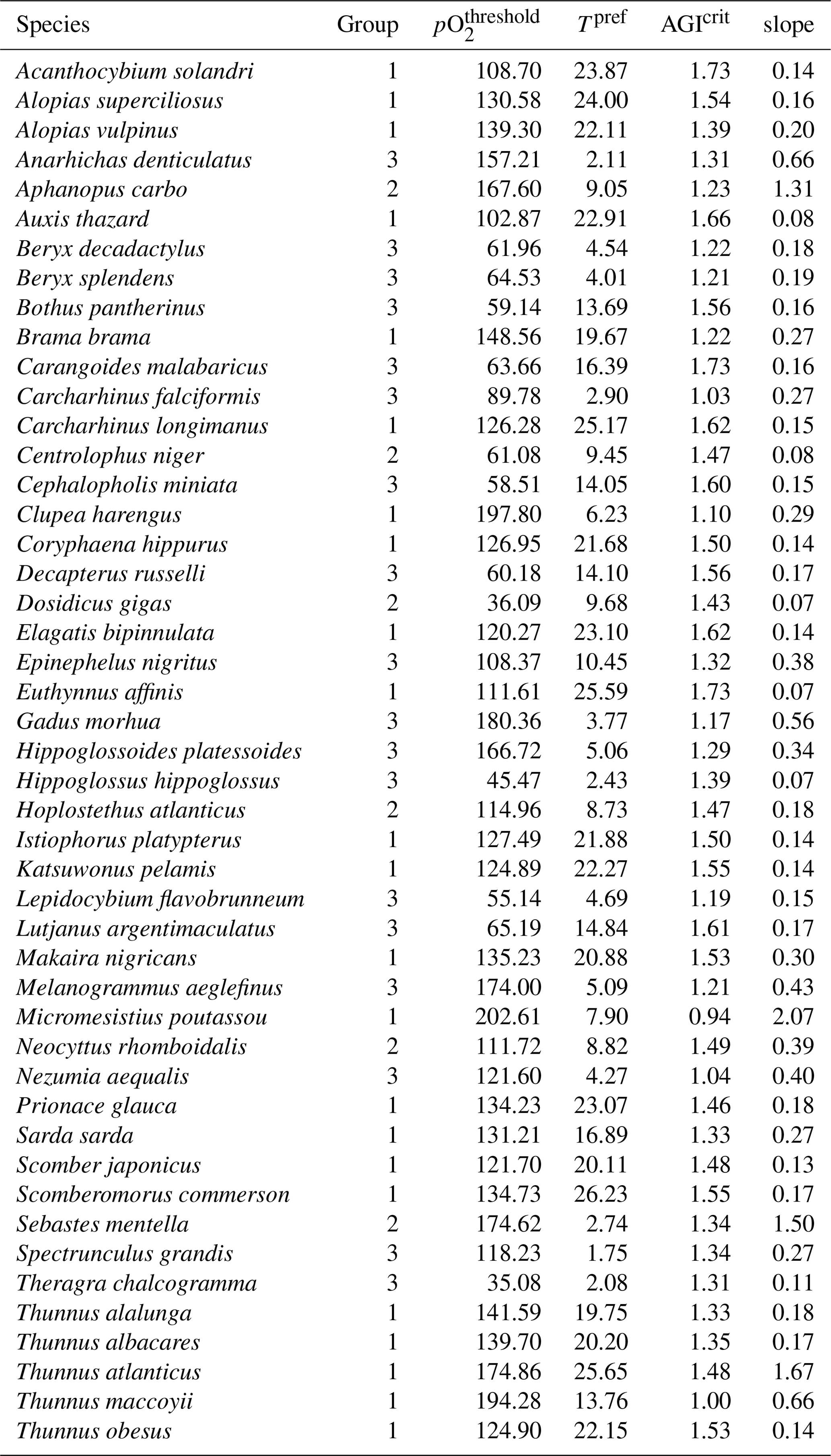
An AGI of 1 implies that there is sufficient O₂ supply for feeding, movement, and defense but not for growth and reproduction. To sustain a viable population, additional aerobic scope is needed until AGI is above its critical value (AGI^crit) for a particular species. Following Clarke et al. (2021), AGI^crit is the 10th percentile of all AGI values in a species' habitat, including vertical and temporal variability, similar to pO${}_{\mathrm{2}}^{\text{threshold}}$ and T^pref. In this study, a species is deemed to be impacted by changes in temperature and pO₂ whenever AGI drops below AGI^crit on an annual mean basis. All species information is listed in Table A1. The coarse resolution and the imperfect harmonization between the biogeographical, temperature, and O₂ data may affect the accuracy of the estimated AGI^crit, as indicated by some species having AGI^crit of or below 1. We discuss in Sect. 4 how such biases may affect the results and conclusion and how future studies can build on our results to improve the accuracy of the analysis.

Relative changes in AGI (AGI^rel) between time = t₁ and time = t₀ can be estimated from Eq. (2):

$$\begin{array}{}\text{(2)}& \begin{array}{rl}{\text{AGI}}^{\text{rel}}=& {\displaystyle \frac{\mathrm{\Delta }\text{AGI}}{\text{AGI}\left(t_{\mathrm{0}}\right)}}={\displaystyle \frac{p{\mathrm{O}}_{\mathrm{2}}\left(t_{\mathrm{1}}\right)}{p{\mathrm{O}}_{\mathrm{2}}\left(t_{\mathrm{0}}\right)}}\\ \cdot & \exp \left(\left(j_{\mathrm{2}}-j_{\mathrm{1}}\right)\cdot \left({\displaystyle \frac{\mathrm{1}}{T\left(t_{\mathrm{1}}\right)}}-{\displaystyle \frac{\mathrm{1}}{T\left(t_{\mathrm{0}}\right)}}\right)\right)-\mathrm{1}\end{array},\end{array}$$

where ΔAGI is AGI(t₁)–AGI(t₀). Relative changes are thus entirely species independent (in contrast to the metabolic index of Deutsch et al., 2015) and are interpreted as relative changes in habitat viability. Eqs. (1) and (2) show that j₂−j₁ (8000–4500 = 3500 K) modulates the influence of the temperature effect on AGI. We maintain a reference period of 1995–2014 throughout this study (i.e., AGI(t₀) is the mean AGI over the years 1995–2014). Individual contributions from pO₂ and temperature to AGI^rel are calculated by keeping temperature or pO₂ constant at its 1995–2014 mean state when calculating AGI^rel.

2.2 Species data

AGI can be calculated for nearly 1000 commercially exploited marine species due to the generalized temperature dependence of the pO${}_{\mathrm{2}}^{\text{demand}}$. This broad applicability of AGI allows us to select 47 representative species (n=47), which are chosen such that depth level, climatic zone (tropical and temperate), and body size are represented. In addition, we selected some pelagic and deep-water wide-ranging species that inhabit both tropical and temperate regions, as well as the hypoxia-tolerant species Dosidicus gigas. Three depth groups are represented through our selection: epipelagic species (n=23) in the 0–200 m depth range, mesopelagic species (n=6) in the 200–1000 m depth range, and demersal species (n=18) at the seafloor (bottom wet layer of the models; Sect. 2.3). The representativeness of our species selection is assessed in Sect. 3.4. Species pO${}_{\mathrm{2}}^{\text{threshold}}$, T^pref, and AGI^crit are listed in Table A1. The contemporary species distributions are based on a gridded product from Close et al. (2006) and are assumed to represent the 1995–2014 mean state (Fig. C1).

2.3 Earth system model data

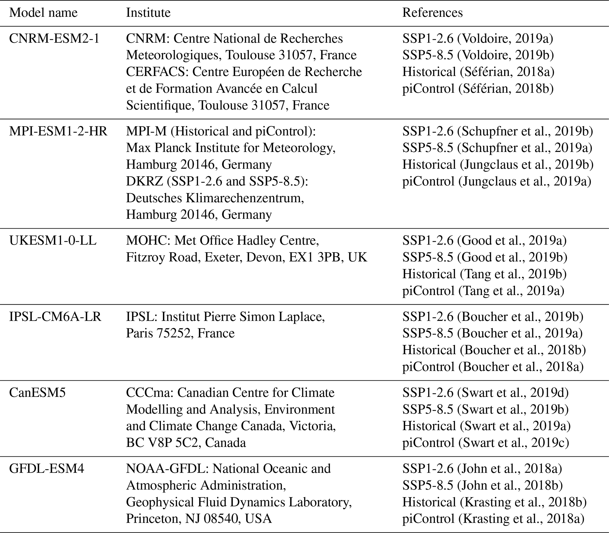
Environmental data of O₂, potential temperature, and salinity for the years 1850–2100 are taken from the Coupled Model Intercomparison Project Phase 6 (CMIP6) multi-model ensemble (Eyring et al., 2016). The historical, SSP5-8.5, and SSP1-2.6 scenarios, as well as the preindustrial control simulation piControl, were used from the following six models for which these environmental data were available: CNRM-ESM2-1, MPI-ESM1-2-HR, UKESM1-0-LL, IPSL-CM6A-LR, GFDL-ESM4, and CanESM5 (Table A2). All model data were horizontally regridded to a 1^∘ regular grid before further post-processing.

To account for mean errors and model drift, both a drift correction and bias correction were performed. First, the bottom layer (seafloor) O₂ ocean data were linearly detrended for piControl drift over the piControl years corresponding to the scenario years (1850 to 2100), as these trends are more than 10 % of the scenario signal for some models. Drift in bottom-layer temperature and salinity, as well as upper-water-column O₂, salinity, and temperature, were negligible compared to the scenario signals and were therefore not accounted for. Secondly, we performed a mean bias correction (e.g., Maraun, 2016) on all model data by subtracting the present-day monthly mean climatological bias (the difference between WOA18 data vertically interpolated to the respective model levels and the respective model's 1995–2014 monthly climatology) from the entire simulated time series. We used the available WOA18 climatological mean product for the seafloor data because WOA18 climatologies are only available at a monthly resolution until 1500 m depth. The extracted original spatial resolution of the WOA18 data is 1^∘ for O₂ and 0.25^∘ for temperature and salinity, but these were all regridded to 1^∘ to match the regridded model data grid. Note that, to calculate the temperature biases, the model potential temperature was converted to in situ temperature. Finally, pO₂ was calculated following Sect. E in Bittig et al. (2018), which is based on earlier work (Benson and Krause, 1984; Garcia and Gordon, 1992; Sarmiento and Gruber, 2006) and includes pressure correction (Taylor, 1978) and the correction for water vapor pressure (Weiss and Price, 1980) in the calculation of pO₂ (Appendix B).

All results are presented at global warming levels (i.e., global mean air temperature at 2 m; e.g., Hausfather et al., 2022). In order to do so, we first bias correct modeled surface air temperatures such that the 1995–2014 global mean air temperature increase since 1850–1900 is 0.87 ^∘C, as observed (HadCRUT.5.0.1.0; Morice et al., 2021), in order to be consistent with the bias-corrected ocean temperature and oxygen data. We then find the first year where the 15-year running mean of these bias-corrected global mean surface air temperature data is greater than or equal to the warming level of interest and calculate the 15-year running mean at that year over the data for the analyses. For warming levels above 1.5 ^∘C, we only use the results for SSP5-8.5, as not all models reach warming of more than 1.5 ^∘C in SSP1-2.6.

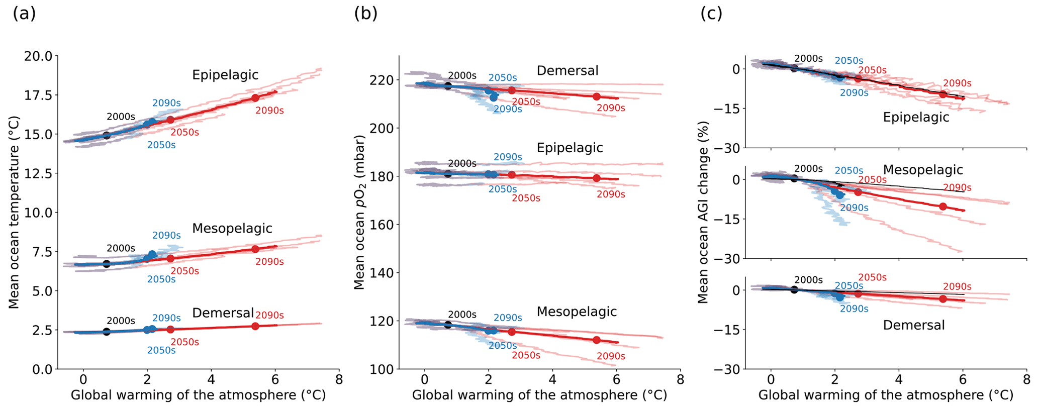
Figure 1 Simulated global mean changes in ocean in situ temperature in ^∘C (a), pO₂ in mbar (b), and AGI^rel in % (c) for different depth layers and global warming levels, where global warming is calculated as the global surface air temperature increase relative to the 1850–1900 mean. The multi-model mean is given in opaque blue (SSP1-2.6) and red (SSP5-8.5) and has, for several decades, the corresponding 20-year multi-model mean year labeled. Individual models are shown in light blue and red without taking a running mean. AGI^rel is given relative to the 1995–2014 mean as in the remainder of the paper, and the mean contribution from temperature only (excluding the small effect of temperature on pO₂) is indicated by the black line in (c) and is calculated by keeping pO₂ constant at its 1995–2014 mean state when calculating AGI^rel. AGI^rel is entirely species independent (Eq. 2), and values that exceed 1000 % or are below −1000 % were excluded during the calculation of the global mean AGI changes to omit several grid cells with extreme outliers caused by very small absolute changes in O₂ causing very large changes in AGI^rel.

3 Results

3.1 Global changes in warming, deoxygenation and habitat viability

Ocean temperature is projected to increase (Fig. 1a) and pO₂ is projected to decrease (Fig. 1b) with global warming of the atmosphere. These changes occur in all three depth layers considered here and for all CMIP6 models. Noticeably, the response of ocean warming and deoxygenation to global atmospheric warming is approximately linear (Fig. 1). From a linear fit to the multi-model mean CMIP6 changes in Fig. 1, we find that the epipelagic realm warms the most, with 0.50 ± 0.03 ^∘C per degree of atmospheric warming (standard deviation given across the individual model fits). This signal is dampened with depth to 0.18 ± 0.02 ^∘C per degree of global warming in the mesopelagic realm and 0.08 ± 0.01 ^∘C per degree of global warming in the demersal realm (Fig. 1a). In addition to the warming, we find that the epipelagic realm loses 0.40 ± 0.55 mbar of pO₂, the mesopelagic loses 1.35 ± 0.89 mbar of pO₂, and the demersal realm loses 1.17 ± 0.97 mbar of pO₂ on average and per degree of global warming of the atmosphere (Fig. 1b). The largest changes in pO₂ are projected at depth in contrast to ocean warming. The warming and deoxygenation reduce AGI relative to its contemporary state (i.e., a negative AGI^rel; Fig. 1c), which we interpret as a loss of habitat viability (Sect. 2.1) that is independent of species (Eq. 2). In the epipelagic, AGI decreases by 2.17 ± 0.69 % per degree of global warming (Fig. 1c), while AGI decreases by 2.33 ± 1.64 % per degree of global warming in the mesopelagic realm. The demersal decrease in AGI is 0.86 ± 0.48 % per degree of global warming, making it the least pronounced of the three studied depth intervals. The approximately linear response of marine warming, deoxygenation, and loss of habitat viability to global atmospheric surface warming (Fig. 1) highlights and confirms that any additionally realized atmospheric warming will affect the marine environment (Cheung et al., 2016).

The projected changes are independent of greenhouse gas emission pathways and only depend on the amount of global warming to a first degree. Even though our results in Fig. 1 are presented at warming levels, here we highlight that the scenario determines the maximum changes in temperature, pO₂, and AGI^rel (Fig. C2): relative to the 1850–1900 mean, global multi-model mean warming by 2081–2100 in SSP1-2.6 is limited to 1.14 ± 0.28 ^∘C in the epipelagic, 0.62 ± 0.07 ^∘C in the mesopelagic, and 0.22 ± 0.02 ^∘C in the demersal realm. For SSP5-8.5, the changes are approximately doubled to 2.70 ± 0.76 ^∘C, 1.00 ± 0.15 ^∘C, and 0.40 ± 0.06 ^∘C of warming, respectively. Deoxygenation is also much reduced in the low-emission scenario as compared to the high-emission SSP5-8.5 scenario by 2081–2100, although model uncertainty is larger here. Global mean pO₂ is reduced by, at most, 0.88 ± 1.42 mbar in the epipelagic, 3.23 ± 2.96 mbar in the mesopelagic, and 5.42 ± 3.80 mbar in the demersal realm for SSP1-2.6, while maximum global mean deoxygenation is projected to be stronger in SSP5-8.5 with losses of 2.27 ± 2.85 mbar, 7.13 ± 4.22 mbar, and 5.61 ± 4.23 mbar pO₂, respectively. The relative loss of habitat viability is 6.39 % lower in SSP1-2.6 than in SSP5-8.5 by 2081–2100 in the epipelagic (−11.58 ± 4.48 % under SSP5-8.5 vs. −5.18 ± 2.08 % under SSP1-2.6), 4.62 % lower in the mesopelagic (−11.48 ± 7.50 % under SSP5-8.5 vs. −6.86 ± 5.60 % under SSP1-2.6), and 0.90 % lower in the demersal realm (−4.23 ± 1.90 % under SSP5-8.5 vs. −3.33 ± 1.69 % under SSP1-2.6).

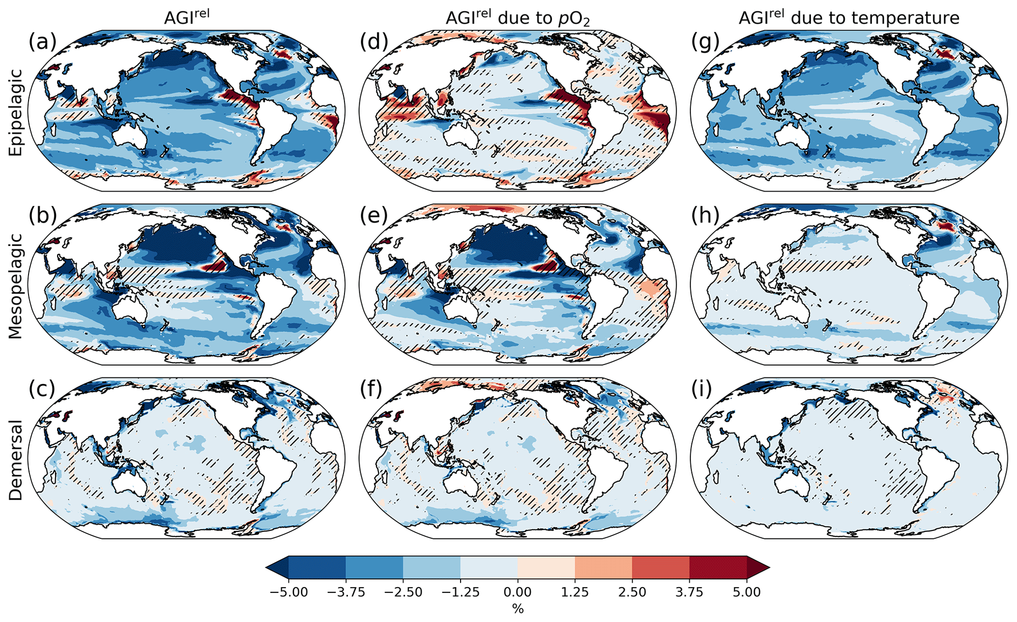
Figure 2 Multi-model mean AGI^rel relative to the 1995–2014 mean at 2 ^∘C global warming (using SSP5-8.5 simulations) vertically averaged over the epipelagic and mesopelagic realms and shown for the demersal realm (a–c). AGI^rel is divided into contributions from (d–f) pO₂ and (g–i) temperature. Data are hatched where more than two out of the six models disagree about the sign of change. Note that seafloor depth and thus demersal depth depend strongly on location. Contributions from pO₂ (temperature) are calculated by keeping temperature (pO₂) constant at its 1995–2014 mean state when calculating AGI^rel. Further note that, since [O₂] depends on temperature too, the contribution to AGI^rel from pO₂ also contains a minor temperature component.

3.2 Local changes and drivers of habitat viability

A relative reduction in habitat viability (i.e., a negative AGI^rel; Fig. 1c) is projected to occur almost everywhere at 2 ^∘C of global warming (Fig. 2a–c; see Figs. C3 and C4 for 1.5 and 3 ^∘C of global warming, respectively), indicating that, for most habitats and therefore most species, we expect a reduction in habitat viability. The relative reduction in habitat viability is generally larger in the epipelagic and mesopelagic realms (Figs. 1c; 2a, b), but the larger spatial heterogeneity at mesopelagic depths reveals that locally mesopelagic AGI reductions may far exceed those in the epipelagic, particularly in the North Pacific (Fig. 2b). Hence, the location of a species' habitat, both vertically and horizontally, is key to projected changes in habitat viability for a specific species. Note that the patterns in each of the panels of Fig. 2 remain similar for higher degrees of global warming; only the intensity of change increases, which agrees with the approximately linear response of the global average AGI^rel to global warming (Fig. 1c).

When considering the contribution from the two drivers of AGI change, pO₂ and temperature changes, AGI^rel is driven mostly by temperature in the epipelagic and by pO₂ in the mesopelagic and demersal realms (Fig. 2d–i). The AGI^rel at 2 ^∘C of global warming due to pO₂ is −0.16 ± 5.12 % for the epipelagic, −2.52 ± 6.96 % for the mesopelagic, and −0.62 ± 2.02 % for the demersal realm (Fig. 2d–f), while the respective AGI^rel due to temperature is −2.32 ± 1.36 %, −0.91 ± 1.18 %, and −0.39 ± 0.95 % (Fig. 2g–i). Hence, ∼94 % of AGI^rel is, on average, driven by the relatively pronounced warming in the epipelagic, since changes in pO₂ are minor (Fig. 1b). This is because the epipelagic realm is generally well ventilated with O₂-rich surface waters. For the mesopelagic (demersal), warming accounts for only 27 % (39 %) of the total AGI^rel. In the mesopelagic, the drivers of loss in habitat viability depend more strongly on location (Fig. 2e, h). The larger contribution from pO₂ to AGI^rel increases the uncertainty for the mesopelagic and demersal realms because model projections are uncertain for pO₂ (Figs. 1b, C5). In some regions, the effects of pO₂ and temperature on AGI^rel may compensate for each other and result in negligible changes in AGI. We find examples of this in the northern Indian Ocean at epipelagic depths, in the Gulf of Guinea at mesopelagic depths, and in the North Atlantic around Iceland at demersal depths.

AGI^rel has large model uncertainty for species that have a large part of their habitat in eastern-boundary upwelling regions or around Antarctica at epipelagic depths, the western equatorial Pacific at mesopelagic depths, north of the Equator in the Indian Ocean at epipelagic and mesopelagic depths, or regions scattered across all ocean basins for demersal depths (hatched areas in Fig. 2a–c). Most of this uncertainty comes from pO₂ (Figs. 2d–f, C5), with temperature contributing to uncertainty in the North Atlantic south of Greenland and in the western equatorial Pacific at mesopelagic depths. Exceptions to the decrease in AGI are limited to some small parts of the world's oceans, including equatorial regions and the North Atlantic south of Greenland in the epi- and mesopelagic,and around the Antarctic continent in the epipelagic. Model disagreement is generally large in these regions of positive AGI^rel and is mostly attributable to projected increases in pO₂, which have large uncertainties (hatching in Fig. 2a–f and model range in Fig. C5).

Besides considering the model uncertainty, we performed a sensitivity analysis of AGI^rel to the choice of generalized temperature dependence parameters (i.e., j₂−j₁). If j₂−j₁ is adjusted to represent an arbitrary low temperature sensitivity of 1000 K, the global mean AGI^rel is 34 % of the standard-case $j_{\mathrm{2}}-j_{\mathrm{1}}=\mathrm{3500}$ K in the epipelagic, 67 % in the mesopelagic, and 73 % in the demersal realm. On the other hand, for an arbitrary high temperature sensitivity ($j_{\mathrm{2}}-j_{\mathrm{1}}=\mathrm{6000}$ K), the global mean AGI^rel is 165 % of the standard-case $j_{\mathrm{2}}-j_{\mathrm{1}}=\mathrm{3500}$ K in the epipelagic, 118 % in the mesopelagic, and 126 % in the demersal realm. Projections for epipelagic species are therefore most sensitive to the choice of j₂−j₁, as temperature changes are largest there. Further work is needed to explore the uncertainty in j₂ and j₁.

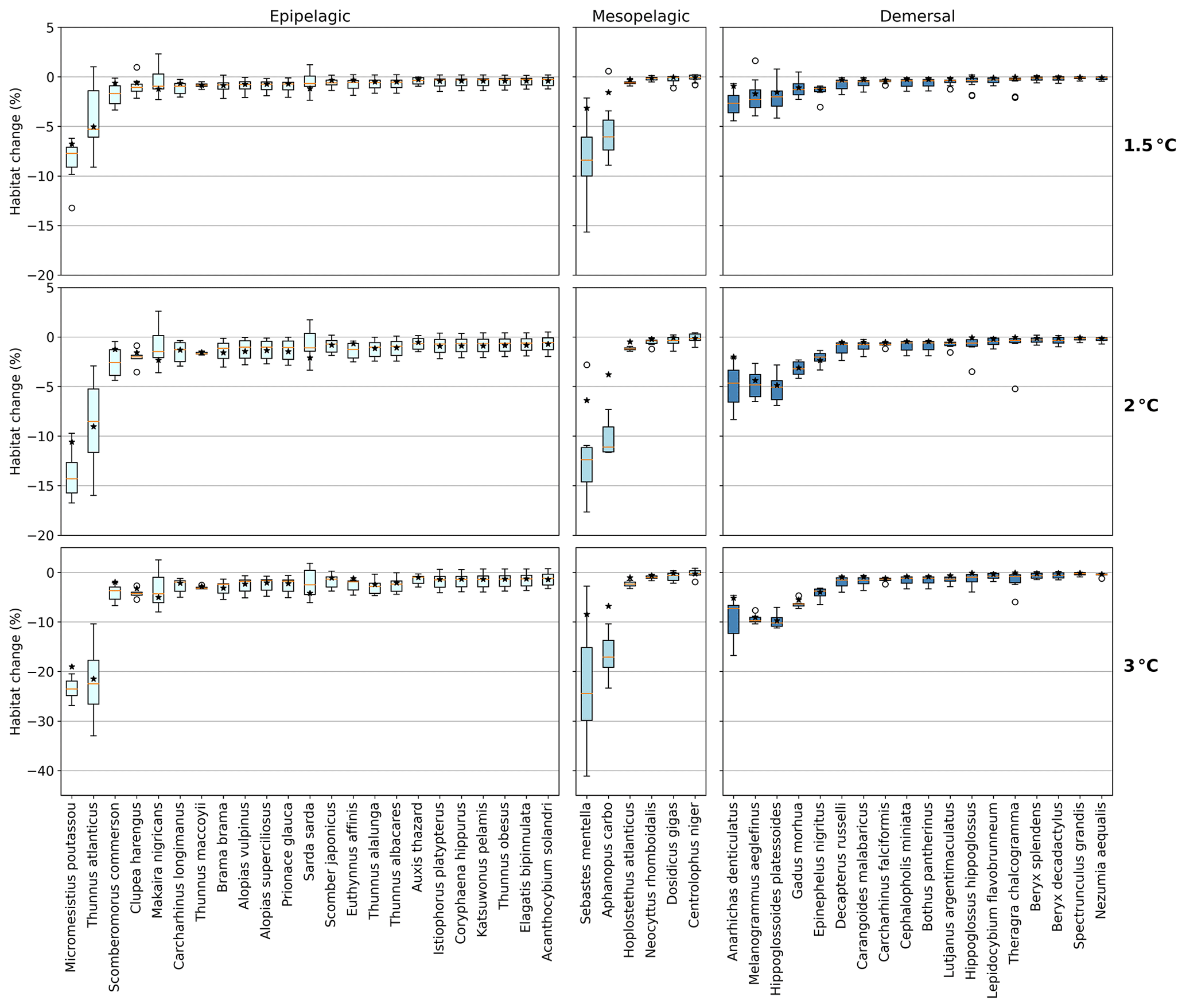
Figure 3 Habitat change (%) of contemporary (1995–2014) habitat volume for different levels of global warming, with negative values indicating habitat loss and positive values indicating habitat gain. Note the different y-axis scale for 3 ^∘C global warming. Habitat volume is considered to be lost when AGI<AGI^crit on an annual mean basis. For 1.5 ^∘C global warming, both the SSP1-2.6 and SSP5-8.5 scenarios are included (number of data points n=2 scenarios × 6 models = 12 for each boxplot), while at higher levels of global warming, we use SSP5-8.5, as not all models reach these warming levels under the SSP1-2.6 scenario (n=6 models). The species are ordered such that species with the largest median losses at 1.5 ^∘C global warming are on the left-hand side for each realm subplot. Each boxplot indicates the median in orange and a box bounded by the interquartile range (IQR; the 25th to 75th percentiles) and the whiskers extending to the data range with a maximum of 1.5×IQR, with outliers as open circles. Stars indicate the median contribution from temperature; the remainder is therefore due to pO₂ changes. As changes are expressed relative to the contemporary viable habitat volume (which is by definition 90 % of the total habitat volume), values up to 10 % (100−90) are possible.

3.3 Impacts of AGI changes on habitat volume of individual species

The overall negative AGI^rel and hence the relative loss of habitat viability with global warming (Figs. 1c and 2) cause a loss of contemporary habitat volume (i.e., newly exposed volume with AGI<AGI^crit) for species at each of the studied depth ranges (Figs. 3 and 4). Habitat loss is expressed relative to its contemporary volume (Fig. 3) to facilitate comparison between wide-ranging and more narrowly distributed species. Loss of contemporary habitat is generally less than 15 % at 2 ^∘C global warming and is mostly under 5 %, but it increases to up to ∼25 % for individual species at 3 ^∘C (Fig. 3). Wide-ranging epipelagic species (e.g., Acanthocybium solandri, Coryphaena hippurus, Katsuwonus pelamis, Thunnus obesus, or Elagatis bipinnulata; Fig. C1) experience losses of contemporary habitat volume of less than 5 % for any of the analyzed warming levels, while more narrowly distributed species experience the largest losses of up to ∼25 % of their contemporary habitat at 3 ^∘C global warming (e.g., Micromesistius poutassou, Thunnus atlanticus, Sebastes mentella, or Anarhichas denticulatus). Notably, species that have the largest contemporary habitat loss at 1.5 ^∘C are generally those species that also lose the most at 3 ^∘C of global warming, which is in line with the earlier findings of the approximately linear response of relative changes in habitat viability to warming and deoxygenation (Fig. 1). Any early (i.e., 1.5 ^∘C) response of a species to warming and deoxygenation is therefore a warning indicator for additional loss of contemporary habitat at increased levels of global warming.

We separately assess the impact of the uncertainty of AGI^crit on these results by calculating habitat loss with an AGI^crit of (a) minimum AGI, (b) 5th percentile, (c) 10th percentile (i.e., the default case), (d) 15th percentile, and (e) 20th percentile of in-habitat AGI. We find that, even when including much higher thresholds (AGI^crit as 20th percentile), our results are similar, with a few species having large losses but most losing less than 5 % at 2 ^∘C of warming relative to the 1995–2014 state (Fig. C6). Moreover, a sensitivity analysis for the species Thunnus atlanticus and Gadus morhua shows that our median result is robust in terms of the choice of the generalized temperature dependence parameters j₂−j₁ (we explored j₂−j₁ ± 71 %; Fig. C7).

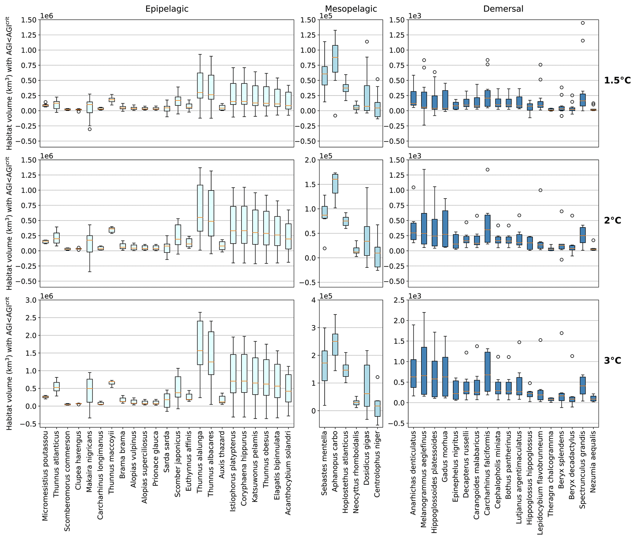
Figure 4 Contemporary habitat loss (km³) for different levels of global warming. Note the different y axes for both the depth groups and warming levels. Habitat volume is considered to be lost when AGI<AGI^crit on an annual mean basis. For 1.5 ^∘C global warming, both the SSP1-2.6 and SSP5-8.5 scenarios are included (number of data points n=2 scenarios × 6 models = 12 for each boxplot), while at higher levels of global warming, we use SSP5-8.5, as not all models reach these warming levels under the SSP1-2.6 scenario (n=6 models). Species are ordered as in Fig. 3. Each boxplot indicates the median in orange and a box bounded by the interquartile range (IQR; the 25th to 75th percentiles) and the whiskers extending to the data range with a maximum of 1.5×IQR, with outliers as open circles.

Absolute losses in habitat volume (i.e., loss expressed in volumetric terms instead of a percentage) show that small relative losses (Fig. 3) often correspond to the largest volumetric losses (Fig. 4). As an example, median Thunnus alalunga habitat loss is less than ∼2.5 % at any of the analyzed warming levels (Fig. 3), while absolute losses are the largest of all 47 species, ranging from 0.25 to 1.5×10⁶ km³ depending on the global warming level (1.5, 2 and 3 ^∘C, Fig. 4). On the other hand, we find species like Sebastes mentella, for which relative losses are large (median 8 %–26 % of the contemporary habitat depending on global warming level; Fig. 3), while absolute losses are comparably small (0.6–1.8×10⁵ km³) because the contemporary volume of Sebastes mentella is relatively small (Fig. 4). Note that epipelagic species lose habitat volume on the order of 1 million km³. In comparison, the entire Black Sea has a volume of about 0.5 million km³. Depending on the location of viable contemporary habitat loss, for species of commercial interest, such a large absolute loss can be particularly impactful to local fisheries.

For most species, temperature is the main driver of habitat loss (black stars in Fig. 3). Exceptions exist, for example, in the mesopelagic, where pO₂ drives about half of the habitat loss for the two species with the largest loss (i.e., Sebastes mentella and Aphanopus carbo), as well as for the demersal species Anarhichas denticulatus. Even though most of the loss can be explained by warming, not all species have large losses despite warming being relatively uniform, although dampened toward depth (Kwiatkowski et al., 2020). These differences can be explained by considering the original spatial and temporal pO₂ and temperature variability in each species' habitat, which shape their vulnerability to change. This is investigated next.

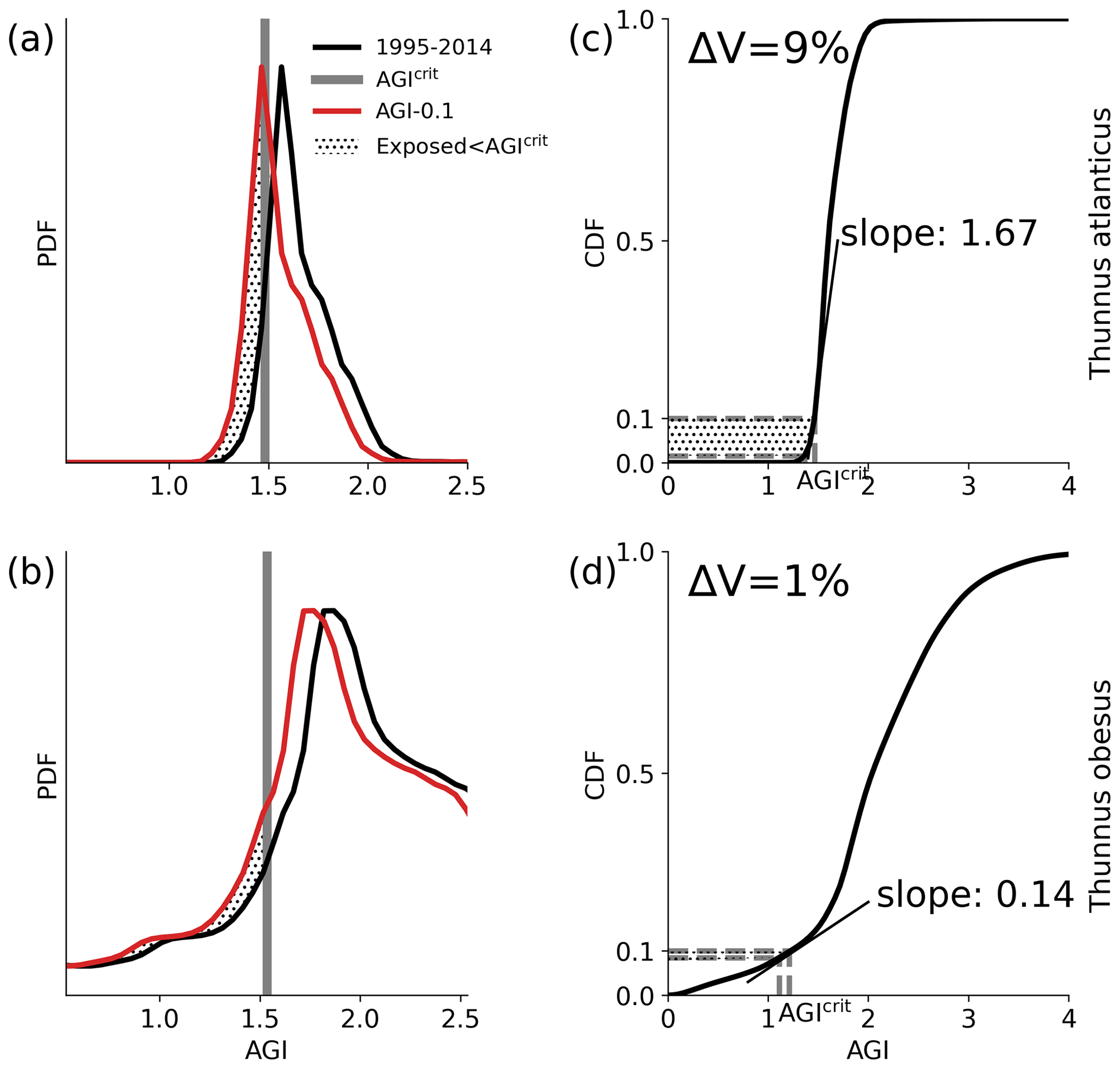
Figure 5 Conceptual figure based on Thunnus atlanticus (a, c) and Thunnus obesus (b, d) showing the difference in impact (change in volume ΔV) of an example mean AGI reduction of 0.1 (i.e., habitat-mean ΔAGI = 0.1) below the 1995–2014 contemporary mean (black lines). This difference is shown to be related to the shape of the PDF and the slope of the CDF at 0.1 (i.e., at AGI^crit), which we refer to as the species vulnerability.

3.4 Drivers of habitat volume loss of individual species

The differences in habitat loss between species as shown in Figs. 3 or 4 are better understood from the probability density of the contemporary (1995–2014) in-habitat AGI for each species (conceptual Fig. 5 and species results in Fig. C8). The spatial variability of the contemporary pO₂ and temperature in each species' habitat results in a species-specific probability density function (PDF) for AGI (black lines in Fig. 5a, b). Depending on this shape, a given reduction in AGI (ΔAGI) exposes a relatively large or small part of the species' habitat to subcritical AGI values (red lines and stippling in Fig. 5a, b), thereby causing volume loss.

We can quantify the vulnerability of a species to changes in AGI by calculating the cumulative sum of the PDFs (i.e., the cumulative density function CDF; conceptual Fig. 5c, d and species-specific results in Fig. C9). The slope of the CDF at a cumulative density of 0.1 (i.e., 10 % of the volume where AGI^crit is defined) indicates the potential loss in habitat for a certain change in AGI (Figs. 5 and C9). If the slope of the CDF is steep at the critical threshold, the species is relatively vulnerable to warming and deoxygenation, as only a small reduction in habitat viability (i.e., AGI) will push a relatively large volume below the critical threshold. An example is given in Fig. 5, where, for an identical change in the mean in-habitat AGI of 0.1, just 1 % of the volume is pushed below AGI^crit for a species with a small slope of 0.14 (Fig. 5b, d, Thunnus obesus), while the same change in AGI results in a 9 % volume loss for a species with a large slope of 1.67 (Fig. 5a, c, Thunnus atlanticus). Changes in the slope of some species' CDFs indicate that different vulnerabilities exist for different parts of that species' habitat (Fig. C9). Hence, in habitat areas that are represented by a part of the CDF with a relatively steep slope, a relatively small change in AGI is needed to bring a relatively large volume closer to AGI^crit. Only the CDF slope at AGI^crit relates directly to viable habitat volume loss, as only AGI values below AGI^crit are considered to have an impact on habitat volume.

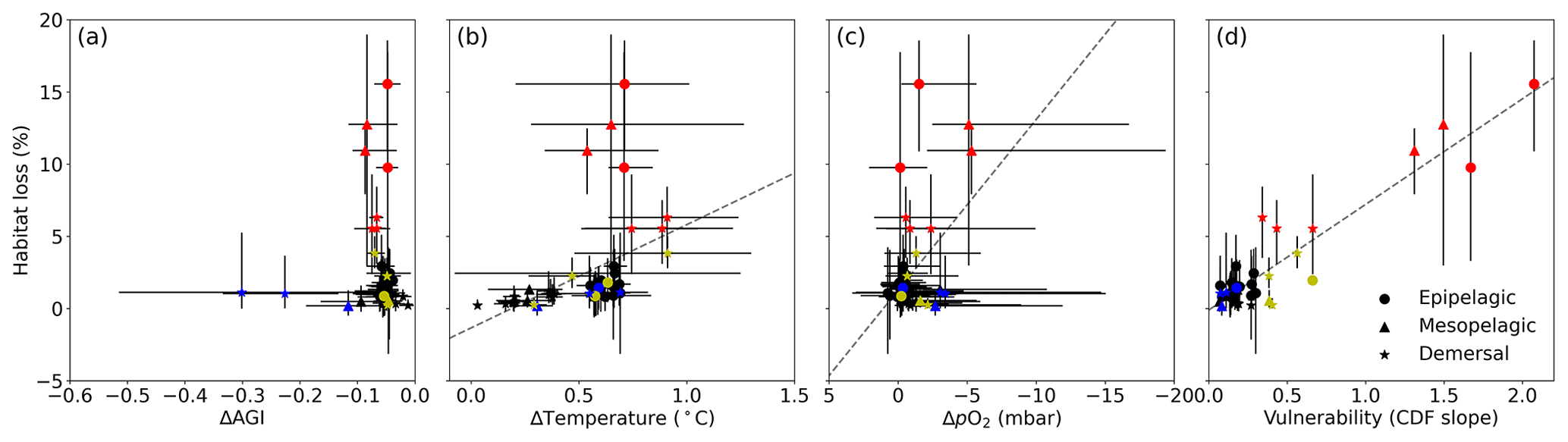
Figure 6 Multi-model mean in-habitat changes at 2 ^∘C of global warming of (a) AGI, (b) temperature, (c) pO₂ (in SSP5-8.5), and (d) vulnerability (CDF slope at a cumulative density of 0.1 based on 1995–2014 mean data – Fig. C9) plotted against loss of contemporary habitat volume for each species (model range indicated by error bars). Species with >5 % loss are marked in red, species with more than −0.1 ΔAGI are marked in blue, and species with volume loss <5 % and vulnerability >0.3 are marked in yellow. There is no uncertainty in the vulnerability calculation because all models have the same 1995–2014 CDF slope due to the WOA18 bias correction. From a linear regression to the data, which is plotted in dashed gray, we find an R² of 0.0 % for (a), the line of which is therefore not plotted; 18 % for (b); 21 % for (c); and 87 % for (d).

Indeed, projected habitat volume loss increases with the species vulnerability (i.e., the CDF slope at AGI^crit; Fig. 6d), as well as, to a lesser extent, with warming and deoxygenation (Fig. 6b, c). Notably, the largest absolute reductions of mean in-habitat AGI do not indicate those species who lose most contemporary habitat volume (Fig. 6a). On the contrary, the environmental state of the contemporary habitat as captured in the PDFs and thus the slope of the CDFs and vulnerability is the strongest indicator of impact; specifically, 87 % of the variance in volume loss at 2 ^∘C global warming can be explained by vulnerability (R² of linear fit in Fig. 6d). This result holds across different levels of global warming. At 1.5 ^∘C of global warming, 85 % of the variance in volume loss can be explained by vulnerability, and at 3 ^∘C of global warming, this is 88 % (see Figs. C10 and C11).

Habitat viability strongly depends on the variability of temperature and O₂ in the habitat of the species, as captured by the species' vulnerability (Figs. 6d and C9). Therefore, reports of relative losses in habitat viability based on pO₂-supply-over-pO₂-demand ratios (e.g., Deutsch et al., 2015; Oschlies, 2021) should not be interpreted as leading to actual reductions of viable habitat for individual species, as they include neither species-specific thresholds nor their vulnerabilities.

We highlight three groups of species for further discussion of the results at 2 ^∘C of global warming: (1) the most affected and vulnerable species due to high vulnerability despite small ΔAGI (red markers in Fig. 6), namely Micromesistius poutassou, Thunnus atlanticus, Sebastes mentella, Aphanopus carbo, Anarhichas denticulatus, Melanogrammus aeglefinus, and Hippoglossoides platessoides; (2) the resilient species which have low losses despite high ΔAGI due to low vulnerability (blue markers in Fig. 6), namely Centrolophus niger, Hippoglossus hippoglossus, and Theragra chalcogramma; and (3) the vulnerable but not-affected species who lose <5 % of their habitat volume due to small ΔAGI despite relatively high vulnerability (yellow markers in Fig. 6), namely Clupea harengus, Thunnus maccoyii, Neocyttus rhomboidalis, Epinephelus nigritus, Gadus morhua, and Nezumia aequalis. Considering the range captured in Fig. 6a–d, we expect that our selection of species is representative of a wide range of marine ectotherms.

Interestingly, species with high vulnerability and loss (red markers in Fig. 6) all have a high pO${}_{\mathrm{2}}^{\text{threshold}}$ above ∼150 mbar (Table A1, Fig. C12). Thus, even though warming explains most of the loss of contemporary habitat, loss is only high for vulnerable species (Fig. 6d) which, in turn, all are sensitive to pO₂, as evidenced by their pO${}_{\mathrm{2}}^{\text{threshold}}$ above ∼150 mbar (Fig. C12). A high sensitivity to pO₂ and hence a high pO${}_{\mathrm{2}}^{\text{threshold}}$ are therefore indicators of vulnerability, although not all species with high pO${}_{\mathrm{2}}^{\text{threshold}}$ are vulnerable (Fig. C12). The high vulnerability for species with a high pO${}_{\mathrm{2}}^{\text{threshold}}$ shows that species in well-oxygenated regions can also be vulnerable to climate change, as their natural pO₂ range is limited. We further note that vulnerability does not depend on the depth realm of a species. Resilient species (blue markers in Fig. 6) have strong spatiotemporal variability in terms of AGI (broad PDF in Fig. C8), such that even large mean changes of AGI (Fig. 6a) do not expose a large volume to subcritical AGI values. Noticeable is that the two species with a PDF skewed to the right (Fig. C8; Hippoglossus hippoglossus and Theragra chalcogramma) are both in this group, while all other species tend to have a left-skewed PDF of AGI values in their habitat. These two species are both demersal dwelling and are very pO₂ tolerant (i.e., low pO${}_{\mathrm{2}}^{\text{threshold}}$; Table A1) and have a wide range of different AGI values in their habitat, with a relatively large volume of high-AGI values causing the right skew (Fig. C8) and resilience (Fig. C12). Whether AGI is the right metric for determining habitat viability for these two species needs further investigation that goes beyond the scope of this study. The six species with relatively high vulnerability but small habitat losses (yellow markers in Fig. 6) experience relatively small AGI changes in their habitats, even at 3 ^∘C global warming (Fig. C8), thereby preventing large habitat losses.

4 Discussion

We introduce a new version of AGI that adds vertical temporal variability in the calculation of pO${}_{\mathrm{2}}^{\text{threshold}}$, T^pref, and AGI^crit, which makes it possible to assess volumetric habitat changes. The original AGI applies and assesses temporal variability in the horizontal direction only (surface or bottom ocean layers for pelagic and demersal species, respectively; Clarke et al., 2021), as commonly practiced (e.g., Bryndum-Buchholz et al., 2019; Tittensor et al., 2021). In other words, either surface or seafloor data were applied for the calculation of pO${}_{\mathrm{2}}^{\text{threshold}}$, T^pref, AGI^crit, and hence AGI in earlier work. To assess the differences between our new approach and the original approach, we repeated the analysis as presented in Fig. 3, now using surface ocean data only for mesopelagic and epipelagic species and calculating pO${}_{\mathrm{2}}^{\text{threshold}}$, T^pref, and AGI^crit from the surface monthly mean WOA18 data only (Fig. C13). We find that the sensitivity to global warming of all species is higher for the original AGI as compared to our new approach, which includes vertical and seasonal variability of temperature and pO₂. This is understood from the combination of (a) the limited spatial variability of surface ocean pO₂ and temperature, which leads to higher T^pref and pO${}_{\mathrm{2}}^{\text{threshold}}$ estimates and therefore a stronger sensitivity to warming and deoxygenation as compared to our new approach, and (b) larger AGI^rel changes closer to the surface. We expect that including temporal and vertical spatial variability in the calculation of AGI provides a more realistic estimate of the pO₂ and temperature variability experienced by a species and therefore a better estimate of its sensitivity to warming and deoxygenation. Nevertheless, we acknowledge that further increasing the spatiotemporal resolution (e.g., using daily mean data and including interannual variability) may increase variability (Deser et al., 2009; Baumann et al., 2015), which can affect estimates of T^pref, pO${}_{\mathrm{2}}^{\text{threshold}}$, and AGI^crit. Unfortunately, no established theory exists yet to decide what temporal variability in environmental parameters best captures species T^pref, pO${}_{\mathrm{2}}^{\text{threshold}}$, or AGI^crit. By considering WOA18 monthly mean climatological data as the basis for our estimates of T^pref, pO${}_{\mathrm{2}}^{\text{threshold}}$, and AGI^crit, we are consistent with the time resolution of the CMIP6 model data (monthly mean).

Regarding the choice of the 10th percentile threshold and the impact of its uncertainty on our results (Fig. C6), we consider an AGI^crit threshold above the 20th percentile of in-habitat AGI values to be unlikely, as then, by definition, already 20 percent of the habitat would be unsuitable to sustain a viable population of that species. Nevertheless, for species where AGI^crit is very close to 1 or even below 1 (Table A1), a higher percentile may be warranted as a meaningful critical value. At the 10th percentile, some uncertainty in the species-specific physiological parameters is considered. We find for most species that the 10th percentile is located at an AGI above which habitat volume steeply increases, suggesting it acts as an appropriate threshold (Fig. C8).

Regarding species data, we assume that our results can be generalized to commercial fish and invertebrates worldwide, as they are based on representative species from different climatic zones (tropical, temperate, polar), vertical habitat (epipelagic, mesopelagic, demersal), geographic range breadths, taxonomic groups (fish and invertebrates), and size classes. Species distribution ranges were generated by an algorithm developed by the Sea Around Us project (see Close et al., 2006; Cheung et al., 2008). The resulting distributions and the parameters used for their construction are available at http://www. seaaroundus.org (last access: July 2008). These distributions have been used to project climate impacts on fishery resources in a great number of studies (Cheung et al., 2009, 2010; Fernandes et al., 2013) and are assumed to represent species distributions over the period 1995–2014 (Tai et al., 2021). Our assumption to extend the 2D distributions provided by Close et al. (2006) over the entire depth range of each species' depth realm is driven by data sparsity and the reliability of 3D species distributions for our selection of species. When reliable 3D habitats, or even time-varying habitats, can be constructed from species observations, these could be included (e.g., distribution data are continuously collected in the Ocean Biodiversity Information System but are currently too sparse to provide 3D distribution data). Some species may be limited to only part of their assigned depth range or may live partly (and possibly temporarily) above or below it. Nevertheless, we expect that the assigned depth range generally provides a good estimate of in-habitat pO₂ and temperature variability, which affects pO${}_{\mathrm{2}}^{\text{threshold}}$, T^pref, and therefore AGI and AGI^crit.

Our results for the mesopelagic include two vertical migrators, (Dosidicus gigas and Aphanopus carbo). As opposed to most other species, the distribution range of vertical migrators is limited at the cold boundary of the distribution because of their low aerobic scope in cold waters (Seibel and Birk, 2022). Therefore, the temperature sensitivity of these species is likely not captured by the generalized temperature dependence in AGI, and contemporary habitat loss due to warming and deoxygenation as estimated for Aphanopus carbo is likely overestimated. We nevertheless project a negligible loss of contemporary habitat for Dosidicus gigas (Fig. 3) due to its low vulnerability and low pO${}_{\mathrm{2}}^{\text{threshold}}$, which is in good agreement with the findings of Seibel and Birk (2022) despite the generalized temperature dependence of AGI. The species-specific thresholds pO${}_{\mathrm{2}}^{\text{threshold}}$ and AGI^crit and preference T^pref are calculated based on the in-habitat spatiotemporal variability of pO₂, temperature, and AGI, respectively. This is done because of the lack of observation-based thresholds and preferences that translate to field conditions (Boyd et al., 2018; Collins et al., 2022).

Detrimental effects from deoxygenation such as reduced vision actually become relevant at much higher pO₂ than at (near-) lethal pO₂ levels (Mccormick and Levin, 2017), while only the latter is often what is assessed in the lab. As an effect, the exact threshold of impact remains unknown and probably depends on many factors, including the impact itself and the abruptness, magnitude, intensity, duration, heterogeneity, and recurrence of exposure to subcritical values (Gruber et al., 2021), as well as the timing of and adaptability to unfavorable temperatures, subcritical pO₂, and hence subcritical AGI.

Through the bias correction of the CMIP6 model data, all monthly mean biases relative to WOA18 are removed from our analysis. We acknowledge the influence of observational uncertainties and the resolution mismatch between our model and the observational WOA18 data used in our bias correction (Casanueva et al., 2020). More complex bias adjustment such as correction for variance biases is prevented by the spatial and temporal resolution of the model and observation data at the global scale. The ongoing effort to collect, compile, and quality control O₂ data in open-access repositories (e.g., Grégoire et al., 2021) will hopefully make it possible to do more advanced bias correction in the future. Until that time, the strong temporal variability and spatial heterogeneity of O₂ trends complicate the comparison between model and observational data. Nevertheless, the remaining forced response of the models likely underestimates deoxygenation (Andrews et al., 2013; Oschlies et al., 2017, 2018; Buchanan and Tagliabue, 2021) and overestimates atmospheric warming (Tokarska et al., 2020) and therefore ocean warming for some CMIP6 models. Part of these warming biases is due to the relatively high climate sensitivities in the CMIP6 models (Meehl et al., 2020). As a further measure to limit model uncertainty, we therefore present results at different global warming levels, such that they are insensitive to the differences in model climate sensitivity (Hausfather et al., 2022). We lastly acknowledge the relatively coarse resolution of the CMIP6 data (typically ca. 100 km in the ocean) which, for species with a highly local distribution (Fig. C1), may lead to higher model uncertainties, especially along the coasts where model disagreement is larger (Fig. C5).

Our approach may give a conservative estimate of contemporary habitat loss, since (a) crossings of the critical thresholds on timescales shorter than 1 year are excluded from our analysis; (b) CMIP6 projections likely underestimate deoxygenation (Andrews et al., 2013; Oschlies et al., 2017, 2018; Buchanan and Tagliabue, 2021), but considering the importance of temperature in driving habitat loss (Fig. 3), especially in the epipelagic realm, the uncertainty of pO₂ projections likely has a relatively small effect on our results; and (c) we do not include other potential stressors on species' habitats in our analysis, such as acidification, net primary production, changes in ecosystem structure, overfishing, marine phenology, disease pressure, food resources, predation pressure, pollution, or eutrophication (e.g., Poloczanska et al., 2016; Bindoff et al., 2019; Whalen et al., 2020). Examples of crossings of the critical thresholds on timescales shorter than 1 year would be short hypoxic events, low-primary-productivity events, and marine heatwaves (Frölicher and Laufkötter, 2018; Jacox et al., 2020; Cheung et al., 2021; Le Grix et al., 2022). Projected deoxygenation and particularly hypoxic or anoxic events have the potential to worsen and even surpass the effects of warming, marine heatwaves, and acidification (Gruber et al., 2021; Sampaio et al., 2021). On the other hand, for some species, the impact will be overestimated if they are able to adapt to future warming and deoxygenation (Cheung et al., 2009; Pinsky et al., 2013; García-Molinos et al., 2016; Palumbi et al., 2019; Collins et al., 2021; Liao et al., 2021). Further note that we considered the potential loss of contemporary habitat only; mobile species have been observed to redistribute based on the rate and direction of climate change (Pinsky et al., 2013), which can preserve the species range area if they are able to expand into newly suitable areas – however, this can alter the original ecosystem structure and function.

For most species, we find a loss of habitat volume of less than 10 %. It is found for example by Gotelli et al. (2021) that only a small percentage of species drives the observed changes in marine species assemblages, showing that even when only a few species experience large losses, impacts can be profound for the ecosystem. For the individual species, however, the loss of only a small fraction of their contemporary habitat likely provides adaptation opportunities. Our results imply that species that are deemed to be vulnerable due to their limited range of in-habitat pO₂ and temperature are likely to be the most impacted by global warming (i.e., vulnerable species in Fig. 6 and species with steep CDF slopes in Fig. C9). Our study can therefore inform e.g., fisheries management by identifying species that are particularly vulnerable to ocean warming and deoxygenation. Such identification provides species-specific information complementing earlier studies that found a reduced impact on fisheries at lower levels of global warming (Cheung et al., 2016). Indeed, for any additional global warming, our study shows increased marine deoxygenation and warming, as well as increased loss of contemporary habitat across all species, albeit with a strongly species-specific magnitude. These results confirm the need to limit global warming levels to the minimum to prevent the loss of contemporary habitat and to support the identification of the species that would be most vulnerable to marine deoxygenation and warming.

5 Conclusions

• Marine warming and deoxygenation are projected to intensify with global warming and drive a relative decrease in global habitat viability, penetrating to all depths (Figs. 1 and 2).

• The generally negative relative changes in habitat viability (i.e., AGI^rel) are dominated by warming at the surface, while deoxygenation becomes increasingly important with depth (Fig. 2).

• Species' loss of contemporary habitat is driven mostly by warming in the epipelagic realm, while in the mesopelagic and demersal realms, reduced pO₂ is also a contributor for some species (Fig. 3).

• Deoxygenation and warming cause most species to lose less than 5 % of their contemporary habitat volume over the 21st century relative to preindustrial levels (Fig. 3). Some individual species are, however, projected to incur losses 2–3 times greater than that at 1.5 and 2 ^∘C of global warming and 4–5 times greater at 3 ^∘C of global warming. At 2 ^∘C of global warming, epipelagic losses are generally on the order of 0.1–0.5 million km³, while mesopelagic losses are on the order of 0.01–0.15 million km³, and demersal losses are on the order of about 0.00025 million km³.

• The impact of negative relative changes in habitat viability (i.e., AGI^rel – Figs. 1c and 2) on lost habitat volume (Figs. 3 and 4) depends on species vulnerability (Figs. 5, 6d, and C9).

• Species vulnerability is shown to be the most important indicator for potential large (>5 %) habitat losses, not relative or absolute changes in AGI, pO₂, or temperature (Fig. 6). A species' pO${}_{\mathrm{2}}^{\text{threshold}}$ being above ∼150 mbar is an indicator for high species vulnerability to warming (Fig. C12). Our approach of quantifying vulnerability can help identify those species most vulnerable to marine warming and deoxygenation.

• We introduce an updated version of AGI. By including temporal and vertical spatial variability in the calculation of the species-specific O₂ thresholds and temperature preference, we include a more realistic representation of the in-habitat variability of O₂ and temperature and therefore likely the species' tolerance to these. The updated AGI has lower sensitivity than in the original AGI of Clarke et al. (2021) (Figs. 3 and C13).

Appendix A: Tables

Table A1 Species information, ordered alphabetically by species name. Group 1 is epipelagic, group 2 is mesopelagic, and group 3 is demersal. pO${}_{\mathrm{2}}^{\text{threshold}}$ (mbar), T^pref(^∘C), and AGI^crit (–) are based on the WOA18 monthly climatology in the habitat (Fig. C1) of the species, except for species in the demersal group, for which only a mean climatology is available (see also Sect. 2.2). The slope (change in fraction of total habitat volume per unit change in habitat-mean AGI at AGI^crit) is calculated from the species' CDF (Sect. 3.4).

Table A2 CMIP6 multi-model data used in this study.

Appendix B: Calculation of pO₂

pO₂ [mbar] at depth (Taylor, 1978, Eq. 5 rewritten; Bittig et al., 2018, Sect. E) can be written as a modified Henry's law as follows:

$$\begin{array}{}\text{(B1)}& p{\mathrm{O}}_{\mathrm{2}}={\displaystyle \frac{\left[{\mathrm{O}}_{\mathrm{2}}\right]}{K_{\mathrm{0}}}}\cdot \exp \left({\displaystyle \frac{V_m\cdot P}{R\cdot T}}\right),\end{array}$$

where $K_{\mathrm{0}}=\frac{{{\mathrm{O}}_{\mathrm{2}}}^{\text{sat}}}{x{\mathrm{O}}_{\mathrm{2}}\cdot (\mathrm{1013.25}-p{\mathrm{H}}_{\mathrm{2}}\mathrm{O})}$, [O₂] is the in situ O₂ concentration (mol kg⁻¹), V_m is the partial molar volume of O₂ ($\mathrm{31.7}\times {\mathrm{10}}^{-\mathrm{6}}$ m³ mol⁻¹; Enns et al., 1965), P is the approximated pressure (Pa; $P=\mathrm{1025}\times \mathrm{9.81}\times \text{depth}$ with depth in m), R is the gas constant (8.3145 m³ Pa K⁻¹ mol⁻¹), T is the absolute temperature (K), O${}_{\mathrm{2}}^{\text{sat}}$ is the saturation O₂ concentration (mol kg⁻¹), xO₂ is the dry-air mole fraction of O₂ in air (0.20946; Glueckauf, 1951), and pH₂O is the water vapor pressure (mbar).

The term $\exp \left(\frac{V_m\cdot P}{R\cdot T}\right)$ (unitless) is the pressure correction term for O${}_{\mathrm{2}}^{\text{sat}}$. We calculate the saturation concentration of O₂ in seawater (Garcia and Gordon, 1992) in mol kg⁻¹ using Eq. (B2):

$$\begin{array}{}\text{(B2)}& {{\mathrm{O}}_{\mathrm{2}}}^{\text{sat}}={\mathrm{10}}^{-\mathrm{6}}\cdot \exp \left(l\right),\end{array}$$

where

$$\begin{array}{rl}& l=A_{\mathrm{0}}+A_{\mathrm{1}}\cdot T_{\text{scaled}}+A_{\mathrm{2}}\cdot T_{\text{scaled}}^{\mathrm{2}}+A_{\mathrm{3}}\cdot T_{\text{scaled}}^{\mathrm{3}}+A_{\mathrm{4}}\cdot T_{\text{scaled}}^{\mathrm{4}}\\ & +A_{\mathrm{5}}\cdot T_{\text{scaled}}^{\mathrm{5}}+\text{salinity}\cdot \left(B_{\mathrm{0}}+B_{\mathrm{1}}\cdot T_{\text{scaled}}+B_{\mathrm{2}}\cdot T_{\text{scaled}}^{\mathrm{2}}+B_{\mathrm{3}}\cdot T_{\text{scaled}}^{\mathrm{3}}\right)\\ & +C_{\mathrm{0}}\cdot {\text{salinity}}^{\mathrm{2}},\end{array}$$

where $T_{\text{scaled}}=\ln \left(\frac{\mathrm{298.15}-T_{\text{in-situ}}}{\text{KC}+T_{\text{in-situ}}}\right)$ and KC = 273.15 K making use of salinity (psu) and in situ temperature T_in-situ (^∘C). The unitless constants A₀₋₅, B₀₋₃, and C₀ are listed in Table B1 (Benson and Krause, 1984; Garcia and Gordon, 1992; Sarmiento and Gruber, 2006).

Table B1 Constants for the calculation of O${}_{\mathrm{2}}^{\text{sat}}$.

We calculate the water vapor pressure pH₂O (mbar) following Weiss and Price (1980) (Eq. B3):

$$\begin{array}{}\text{(B3)}& \begin{array}{rl}p{\mathrm{H}}_{\mathrm{2}}\mathrm{O}=& \mathrm{1013.25}\cdot \exp (D_{\mathrm{0}}+D_{\mathrm{1}}\cdot {\displaystyle \frac{\mathrm{100}}{T_{\text{in-situ}}+\text{KC}}}\\ +& D_{\mathrm{2}}\cdot \ln \left({\displaystyle \frac{T_{\text{in-situ}}+\text{KC}}{\mathrm{100}}}\right)+D_{\mathrm{3}}\cdot \text{salinity}),\end{array}\end{array}$$

with D₀=24.4543, $D_{\mathrm{1}}=-\mathrm{67.4509}$, $D_{\mathrm{2}}=-\mathrm{4.8489}$, and $D_{\mathrm{3}}=-\mathrm{5.44}\times {\mathrm{10}}^{-\mathrm{4}}$ .

Appendix C: Additional figures

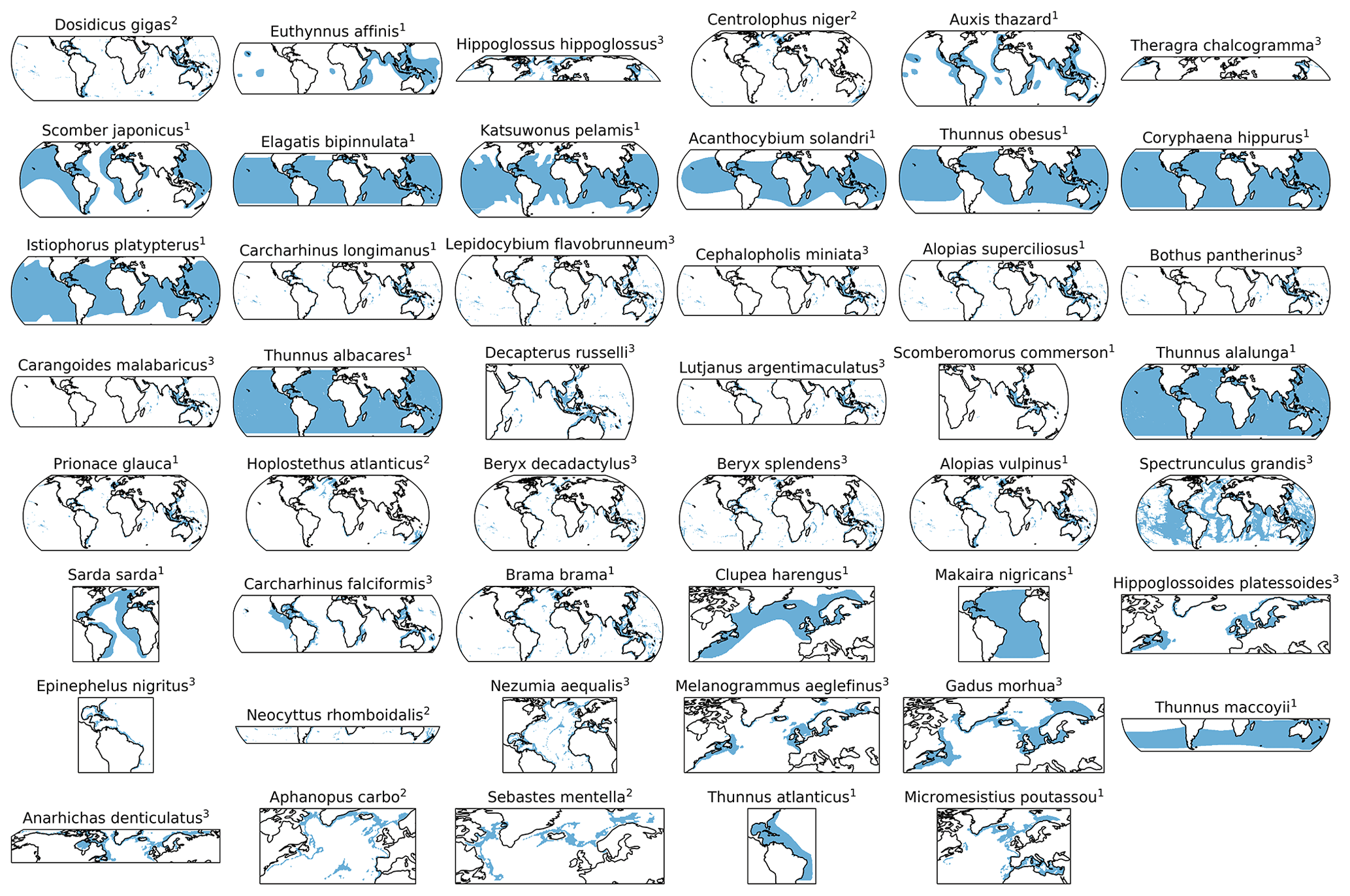
Figure C1 Horizontal distributions for each species in blue based on Close et al. (2006), with superscript indicating the species' depth realm, as in Table A1 (1 = epipelagic, 2 = mesopelagic, 3 = demersal). Species are ordered based on the slope of the CDF (Fig. C9). These 2D habitats were extended over the depth range of the respective species' group for the analysis (Sect. 2.2).

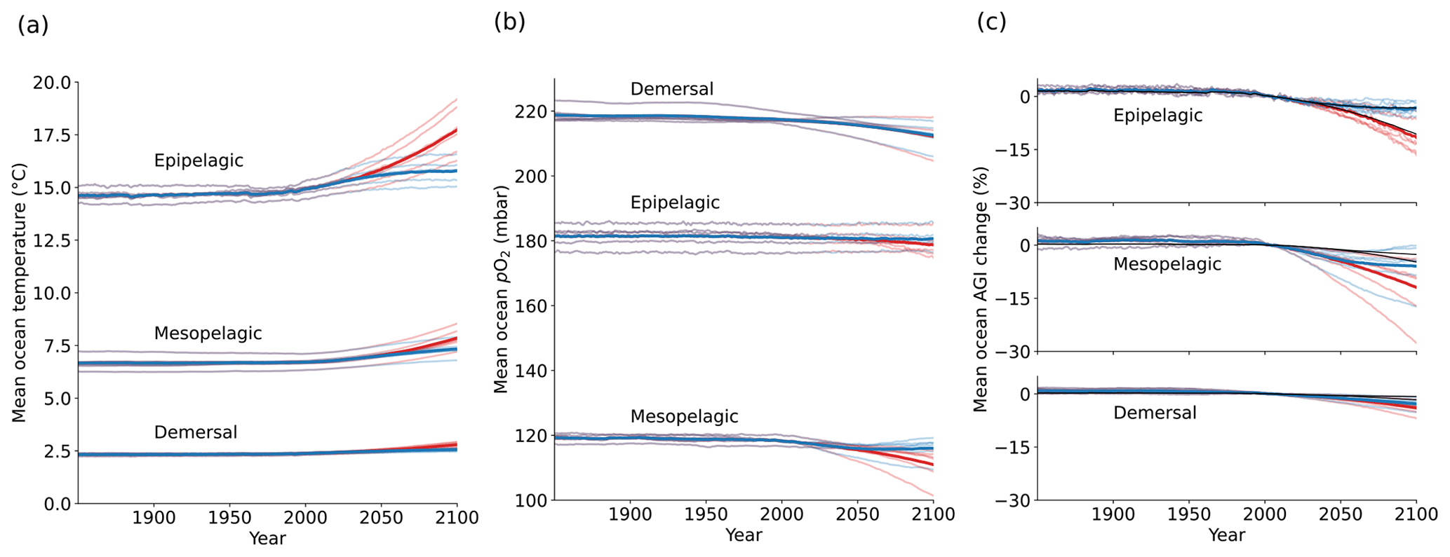
Figure C2 Global mean changes in ocean in situ temperature in ^∘C (a), pO₂ in mbar (b), and AGI^rel in % (c) for years 1850–2100. The multi-model mean is given in opaque blue (SSP1-2.6) and red (SSP5-8.5). Individual models are shown in light blue and red without taking a running mean. AGI^rel is given relative to the 1995–2014 mean, and the mean contribution from temperature only (excluding the small effect of temperature on pO₂) is indicated by the black line in (c) and is calculated by keeping pO₂ constant at its 1995–2014 mean state when calculating AGI^rel. AGI^rel is entirely species independent (Eq. 2), and values that exceed 1000 % or are below −1000 % were excluded during the calculation of the global mean AGI changes to omit several grid cells with extreme outliers caused by very small absolute changes in O₂ causing very large changes in AGI^rel.

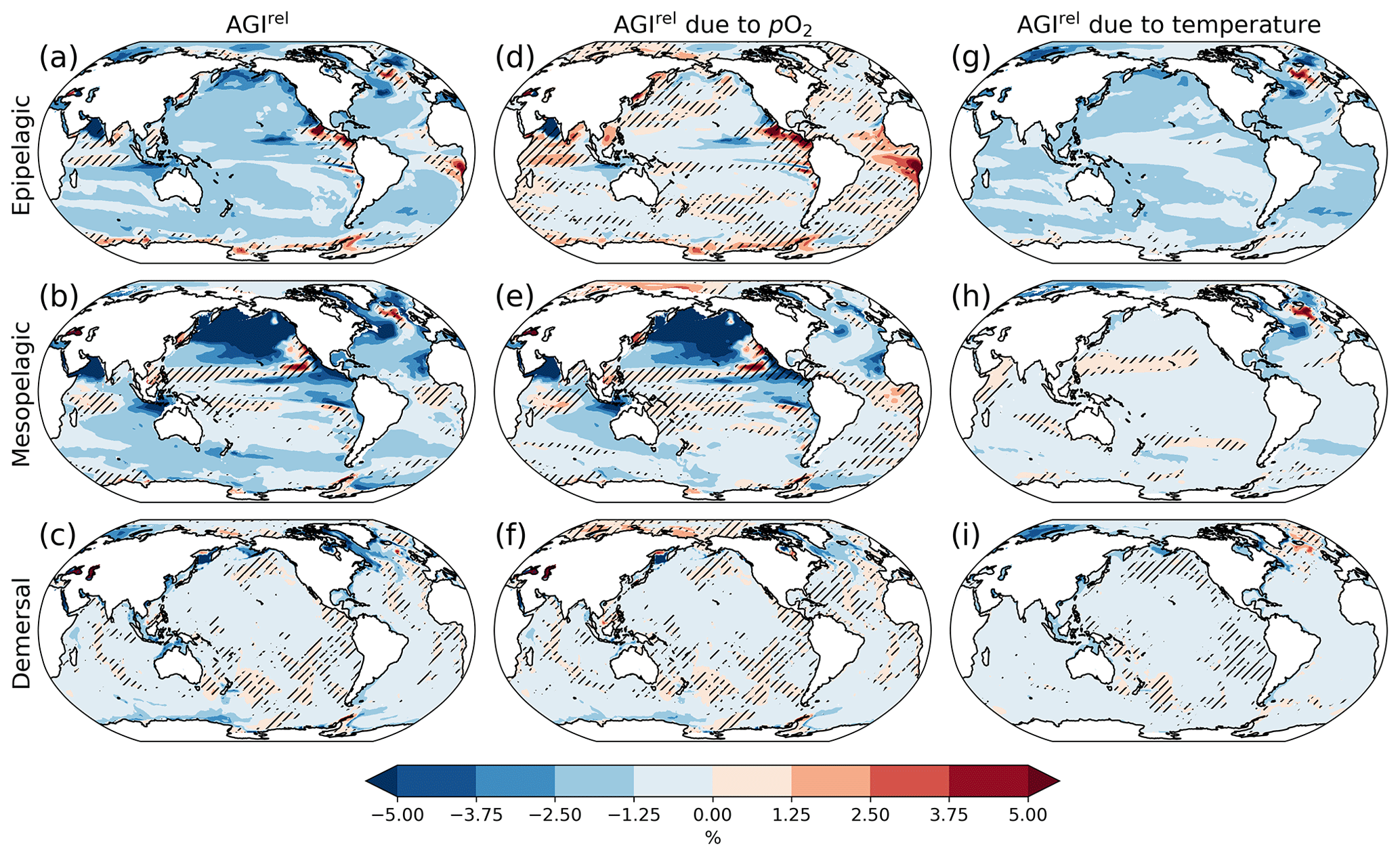
Figure C3 Multi-model mean AGI^rel relative to the 1995–2014 mean at 1.5 ^∘C global warming (using the mean of the SSP1-2.6 and SSP5-8.5 simulations), vertically averaged over the epipelagic and mesopelagic realms and shown for the demersal realm (a–c). AGI^rel is split up into the contribution from (d–f) pO₂ and (g–i) temperature. Data are hatched where the scenario means of more than two out of the six models disagree about the sign of change. Note that seafloor depth and thus demersal depth depend strongly on location. Contributions from pO₂ (temperature) are calculated by keeping temperature (pO₂) constant at its 1995–2014 mean state when calculating AGI^rel. Further note that, since [O₂] depends on temperature too, the contribution to AGI^rel from pO₂ also contains a minor temperature component.

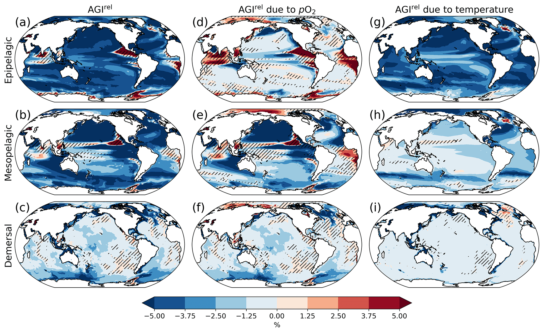
Figure C4 Same as Fig. C3 but for 3 ^∘C global warming (and therefore using SSP5-8.5 simulations only).

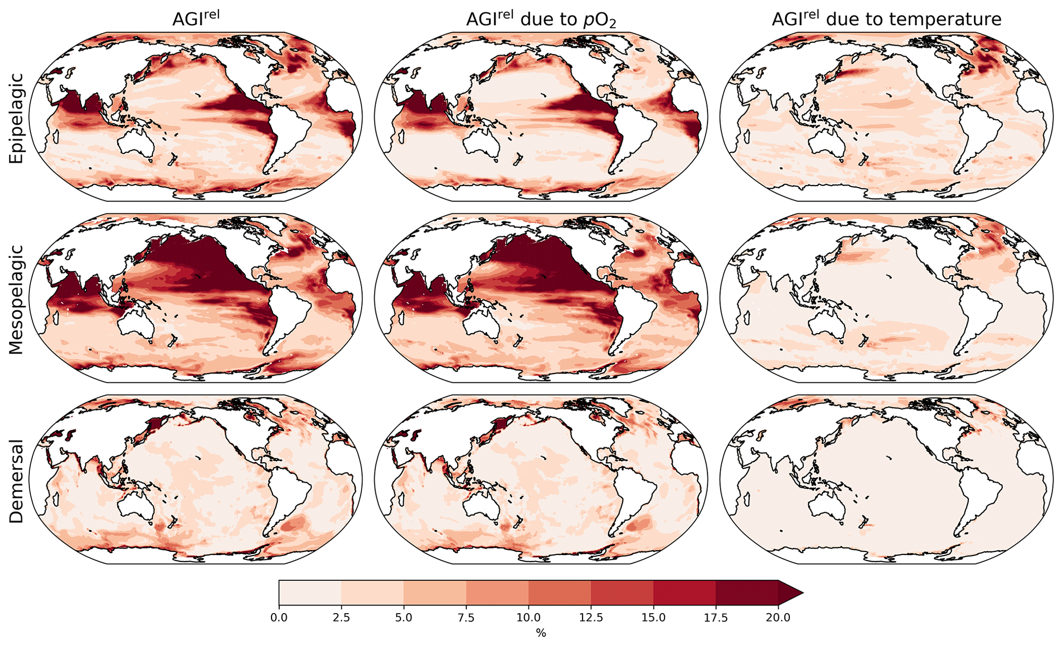
Figure C5 Multi-model range of AGI^rel at 2 ^∘C global warming for the three depth intervals studied.

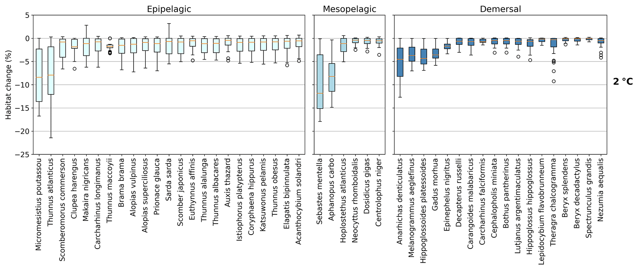
Figure C6 Habitat change (%) of contemporary (1995–2014) habitat volume for 2 ^∘C global warming, including five levels of AGI^crit in every species' boxplot (number of data points n=5 AGI^crit levels × 6 models = 30); AGI^crit is taken as the minimum in-habitat AGI value, the 5th percentile, the 10th percentile, the 15th percentile, and the 20th percentile, respectively. Note the different y axis when comparing to Fig. 3. Each boxplot indicates the median in orange and a box bounded by the interquartile range (IQR; the 25th to 75th percentiles) and the whiskers extending to the data range with a maximum of 1.5×IQR, with outliers as open circles.

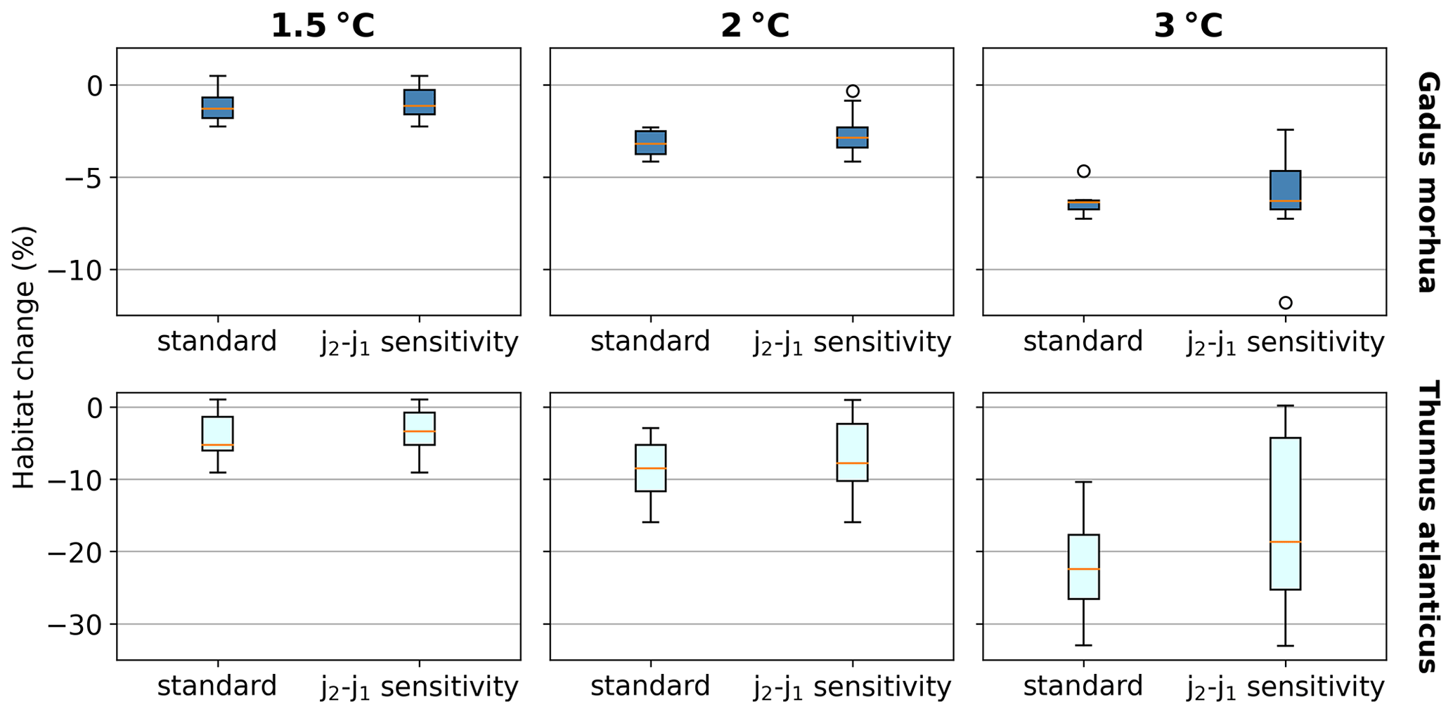
Figure C7 Habitat change (%) sensitivity to the choice of j₂−j₁ for the species Gadus morhua and Thunnus atlanticus. Standard results are as in Fig. 3 and use the standard $j_{\mathrm{2}}-j_{\mathrm{1}}=\mathrm{3500}$ K (Sect. 2.1). For j₂−j₁ sensitivity, j₂−j₁ is adjusted to represent a low (high) temperature sensitivity of 1000 K (6000 K), which is equivalent to varying the standard j₂ and j₁ by ±20 % (resulting in the difference of j₂−j₁ being varied by ±71 %) and recalculating AGI, AGI^crit, and volume loss for each j₂−j₁. The standard, low, and high j₂−j₁ are all included in the j₂−j₁ sensitivity boxplots.

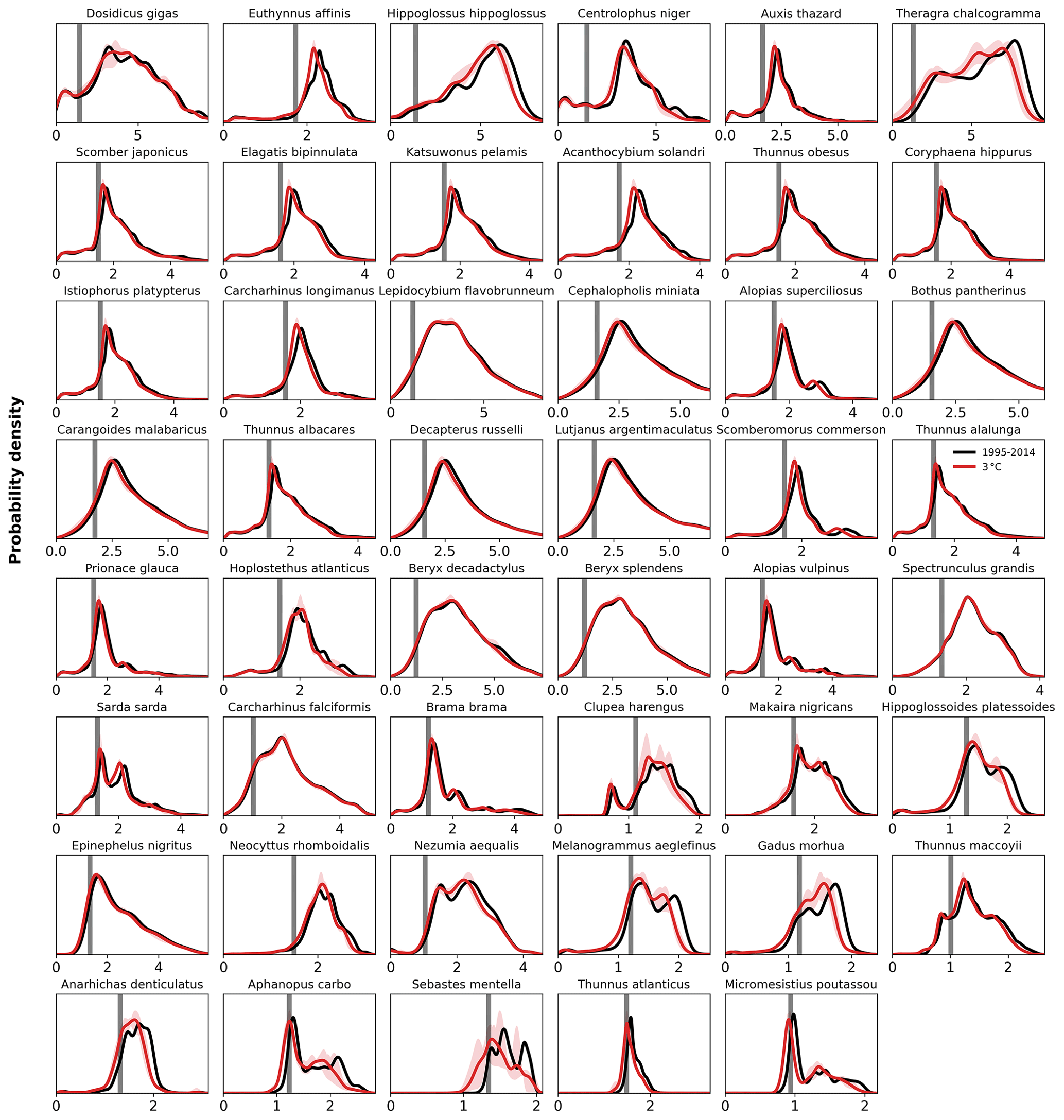
Figure C8 Probability density of AGI for each species for the contemporary reference period 1995–2014 (in black) and for 3 ^∘C global warming (in red with shaded model range). The PDF is a kernel density estimate using Gaussian kernels, calculated using Python's SciPy package function gaussian_kde with grid cell volume taken as weights, following Scott's Rule, and evaluated at 50 000 points from an AGI of 0 to 25. Species are ordered based on the slope of the CDF (Fig. C9).

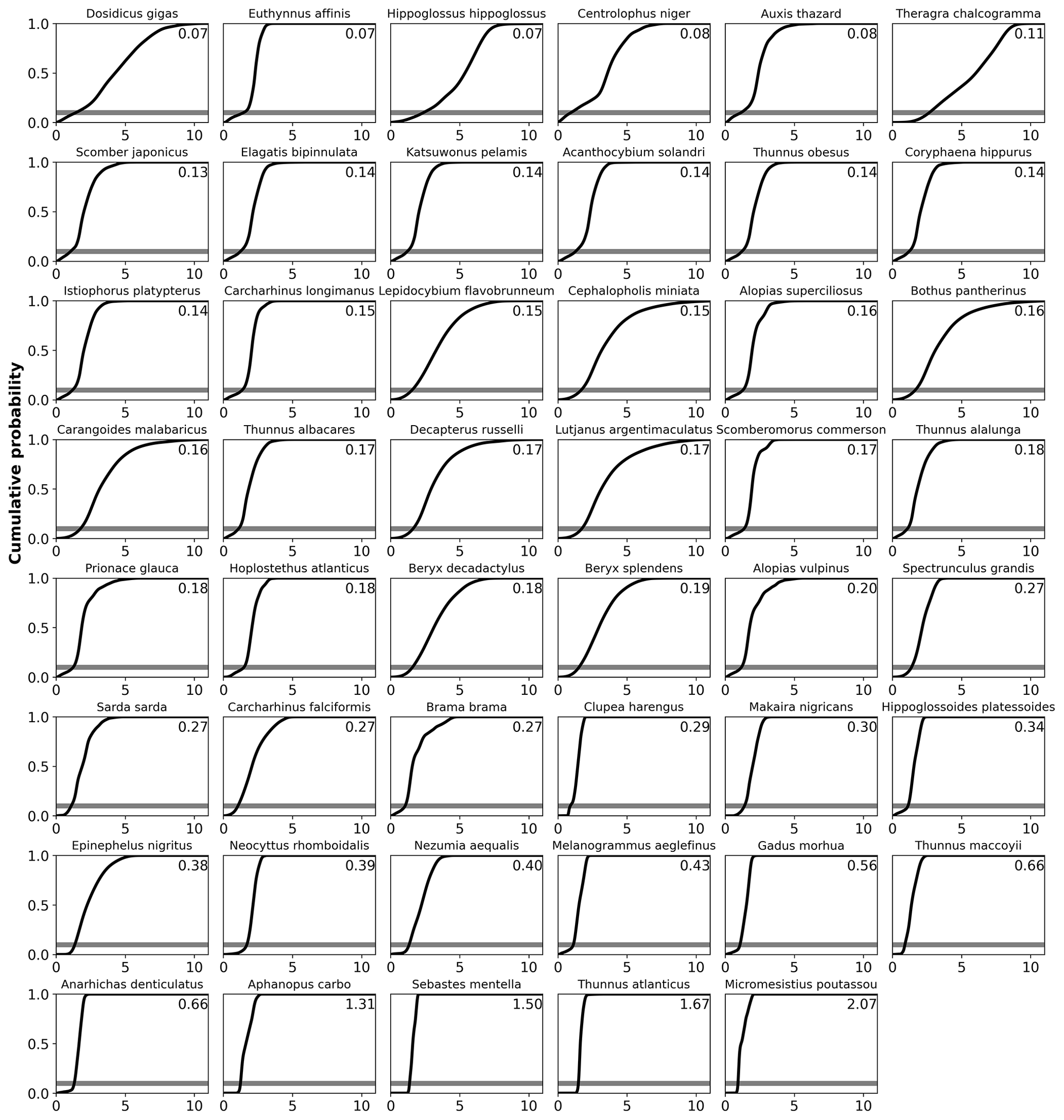
Figure C9 Cumulative density function of AGI at 1995–2014 for each species with vulnerability annotated in upper-right corner (slope at cumulative density of 0.1, i.e., at AGI = AGI^crit). The cumulative density is calculated as the cumulative sum of the probabilities in the PDF estimate (Fig. C8), normalized to a sum of 1. Species are ordered based on their slope.

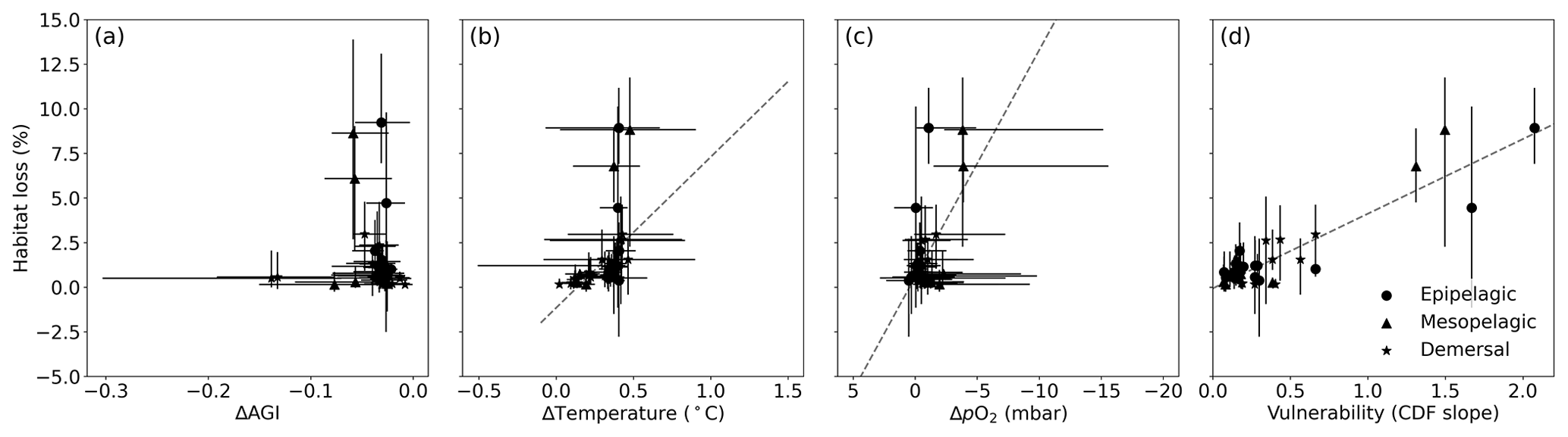
Figure C10 Multi-model mean in-habitat changes at 1.5 ^∘C of global warming of (a) AGI, (b) temperature, (c) pO₂ (mean over SSP1-2.6 and SSP5-8.5), and (d) vulnerability (CDF slope at a cumulative density of 0.1 based on 1995–2014 mean data; Fig. C9) plotted against loss of contemporary habitat volume for each species (model range indicated by error bars). There is no uncertainty in the vulnerability calculation because all models have the same 1995–2014 CDF slope due to the WOA18 bias correction. From a linear regression to the data, which is plotted in dashed gray, we find an R² of 0.0 % for (a), the line of which is therefore not plotted; 25 % for (b); 27 % for (c); and 85 % for (d).

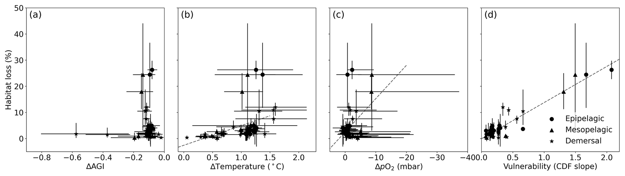
Figure C11 Same as Fig. C10 but for 3 ^∘C global warming (and therefore using SSP5-8.5 simulations only). We find an R² of 0.0 % for (a), the line of which is therefore not plotted; 20 % for (b); 17 % for (c); and 88 % for (d).

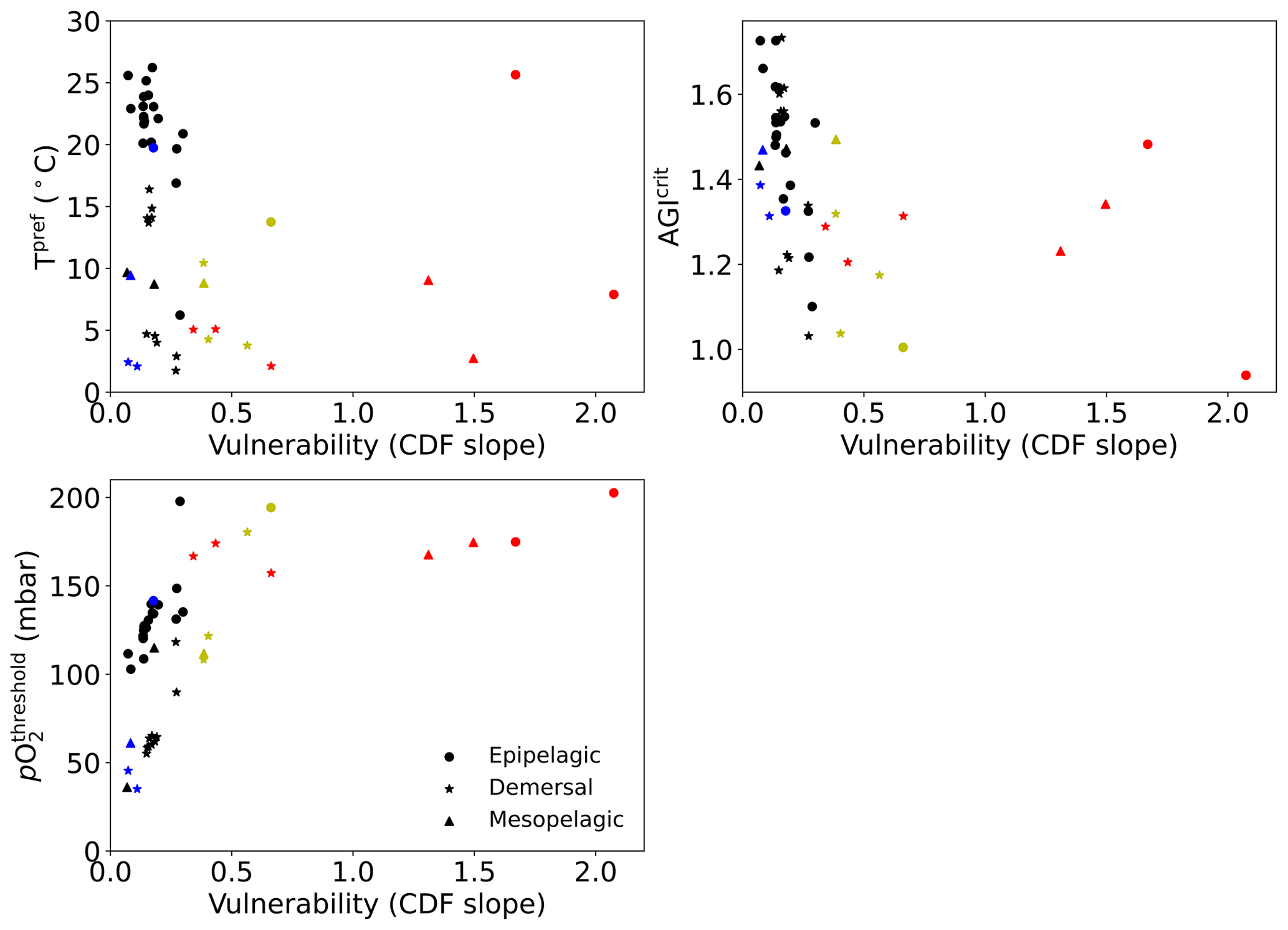
Figure C12 For each species T^pref, AGI^crit, and pO${}_{\mathrm{2}}^{\text{threshold}}$ (see also Table A1) plotted against their vulnerability (slope at cumulative density of 0.1, i.e., at AGI = AGI^crit; see also Figs. C9, 6; Table A1). Colors as in Fig. 6: for 2 ^∘C global warming, species with >5 % loss are marked in red, species with more than −0.1ΔAGI are marked in blue, and species with volume loss <5 % and vulnerability >0.3 are marked in yellow.

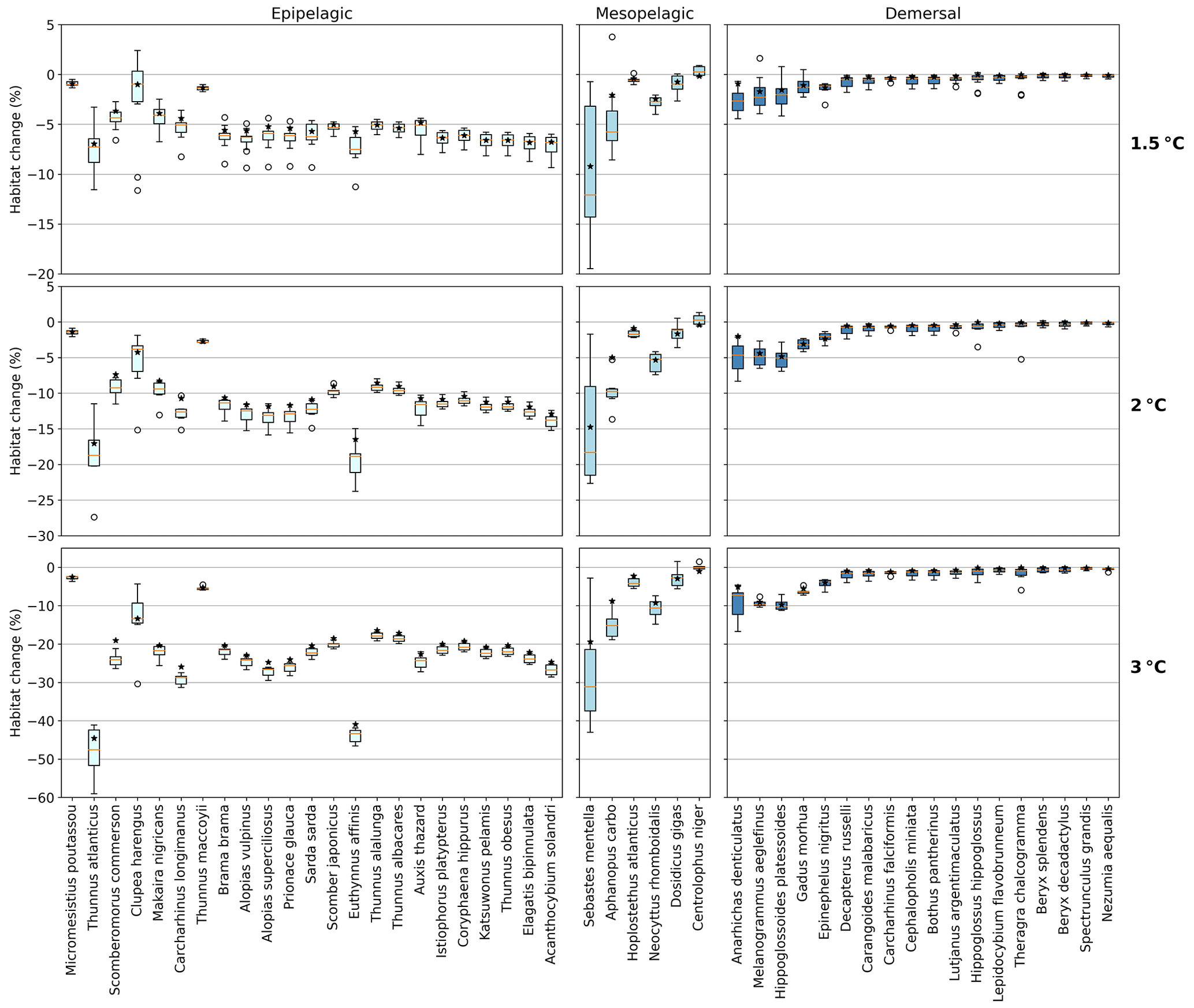
Figure C13 Habitat change (%) of contemporary (1995–2014) habitat volume for different levels of global warming, with negative values indicating habitat loss and positive values indicating habitat gain. This figure is the same as Fig. 3, but here, only surface values are applied in calculating pO${}_{\mathrm{2}}^{\text{threshold}}$, T^pref, and AGI^crit and, hence, AGI and volume <AGI^crit. Demersal results are logically the same as in Fig. 3, as these consider only the seafloor. Note the different y axes (also when comparing to Fig. 3). Each boxplot indicates the median in orange and a box bounded by the interquartile range (IQR; the 25th to 75th percentiles) and the whiskers extending to the data range with a maximum of 1.5×IQR, with outliers as open circles. As changes are expressed relative to the contemporary viable habitat volume (which is, by definition, 90 % of the total habitat volume), values up to 10 % ($=\mathrm{100}-\mathrm{90}$) are possible.