the Creative Commons Attribution 4.0 License.
the Creative Commons Attribution 4.0 License.
 | 06 Jul 2023
Importance of multiple sources of iron for the upper-ocean biogeochemistry over the northern Indian Ocean
Priyanka Banerjee
Although the northern Indian Ocean (IO) is globally one of the most productive regions and receives dissolved iron (DFe) from multiple sources, there is no comprehensive understanding of how these different sources of DFe can impact upper-ocean biogeochemical dynamics. Using an Earth system model with an ocean biogeochemistry component, this study shows that atmospheric deposition is the most important source of DFe to the upper 100 m of the northern IO, contributing more than 50 % of the annual DFe concentration. Sedimentary sources are locally important in the vicinity of the continental shelves and over the southern tropical IO, away from high atmospheric depositions. While atmospheric depositions contribute more than 10 % (35 %) to 0–100 m (surface-level) chlorophyll concentrations over large parts of the northern IO, sedimentary sources have a similar contribution to chlorophyll concentrations over the southern tropical IO. Such increases in chlorophyll are primarily driven by an increase in diatom population over most of the northern IO. The regions that are susceptible to chlorophyll enhancement following external DFe additions are where low levels of background DFe and high background nitrate-to-iron values are observed. Analysis of the DFe budget over selected biophysical regimes over the northern IO points to vertical mixing as the most important mechanism for DFe supply, while the importance of advection (horizontal and vertical) varies seasonally. Apart from removal of surface DFe by phytoplankton uptake, the subsurface balance between DFe scavenging and regeneration is crucial in replenishing the DFe pool to be made available to the surface layer by physical processes.
- Article
(6026 KB) - Full-text XML
-
Supplement
(3848 KB) - BibTeX
- EndNote


Iron is an essential micronutrient for primary producers in the ocean due to the catalytic role of iron in photosynthesis, respiration, and nitrogen fixation (Geider and La Roche, 1994; Raven, 1988). Although iron is one of the most abundant elements in the Earth's crust (McLennan, 2001), its low solubility (Sholkovitz et al., 2012) coupled with an intricate balance between complexation by ligands and a high scavenging tendency does not make it readily bioavailable (Boyd and Ellwood, 2010). It has been estimated that iron availability limits primary productivity in as much as ∼ 30 % of the global oceans, which results in accumulation of unutilized macronutrients like nitrate and phosphate (C. M. Moore et al., 2013). Even in regions experiencing nitrate limitation of productivity, nitrogen fixation is controlled by the supply of iron (e.g., Mills et al., 2004; Moore et al., 2009; Schlosser et al., 2014). Several artificial iron addition experiments performed in the open oceans have demonstrated its significance in regulating phytoplankton growth (Yoon et al., 2018), while natural iron fertilizations have also shown high levels of carbon export from the upper ocean following increased productivity (e.g., Blain et al., 2007; Pollard et al., 2009).
The main external sources of dissolved iron (DFe) to the world oceans are atmospheric depositions (e.g., Conway and John, 2014; Jickells et al., 2005), continental sediments (Elrod et al., 2004; Johnson et al., 1999), river inputs (e.g., Buck et al., 2007; Canfield, 1997), sea ice (Sedwick and DiTullio, 1997; Wang et al., 2014), and iron seeping from hydrothermal vents (e.g., Nishioka et al., 2013; Tagliabue et al., 2010). Most ocean biogeochemistry models simulating the iron cycle estimate dust (1.4–32.7 Gmol yr−1) or sedimentary sources (0.6–194 Gmol yr−1) to have the highest contribution to the ocean DFe inventory (Tagliabue et al., 2016). However, many of these models do not include hydrothermal sources of DFe. Numerical modeling using dust and sedimentary and hydrothermal sources of DFe has shown that, while the ocean column DFe inventory is most sensitive to sedimentary and hydrothermal DFe, atmospheric and sedimentary sources of DFe have the largest impact on atmospheric carbon dioxide (Tagliabue et al., 2014). This is because, while atmospheric and sedimentary DFe can impact productivity over both the open and coastal oceans, iron from hydrothermal vents reaching the surface water depends on deepwater ventilation and the stabilizing impact of organic ligands (Tagliabue et al., 2010; Sander and Koschinsky, 2011). However, with the availability of more in situ DFe measurements, the relative importance of different sources of DFe is being re-examined at global and regional scales.
The northern Indian Ocean (IO) is one of the most productive regions of the global oceans, contributing high levels of organic carbon fluxes to the deeper ocean (e.g., Barber et al., 2001; Madhupratap et al., 2003; Rixen et al., 2019). The monsoonal winds drive phytoplankton blooms over different regions of the northern IO, arising from distinct physical mechanisms in different seasons. These mechanisms include blooms due to coastal and open-ocean upwelling, advection of nutrients by ocean currents, and mixed-layer deepening by winter convection. Episodic blooms are also triggered by the passage of cyclones (Kuttippurath et al., 2021) and mesoscale eddies (Prasanna Kumar et al., 2004; Vidya and Prasanna Kumar, 2013). The region hosts one of the most intense oxygen-minimum zones of the world oceans (Schmidtko et al., 2017) and is globally one of the major denitrification sites (e.g., Morrison et al., 1999; Bianchi et al., 2012). Several water column measurements have shown that the primary limiting nutrient over the northern IO is reactive nitrogen, with possible co-limitation by silicate (Końe et al., 2009; C. M. Moore et al., 2013; Morrison et al., 1998). In recent years, a few studies using ocean biogeochemistry models have also pointed to possible iron limitation of phytoplankton blooms during southwest monsoon months (June–September), especially over the upwelling regions of the western Arabian Sea (AS), which is the northwestern part of the IO (Końe et al., 2009; Wiggert and Murtugudde, 2007). These findings on the role of iron limitation have also been supported by incubation experiments over the AS during the late southwest monsoon, which noted chlorophyll enhancements following iron enrichments (Moffett et al., 2015). Furthermore, in situ measurements during the late southwest monsoon have revealed complete drawdowns of silicate owing to its high utilization under iron limitation, as well as high nitrate-to-iron ratios over the western AS (Naqvi et al., 2010). Nutrient enrichment experiments over the central AS during northeast monsoon months (December–March) have also revealed signatures of iron and nitrate co-limitation, with the addition of these two nutrients supporting increases in diatoms and coccolithophores (Takeda et al., 1995). Co-limitation by nitrogen, phosphorus, and iron has been identified over the southern Bay of Bengal (BoB, the northeastern part of the IO) and the eastern equatorial IO (Twining et al., 2019). Thus, the availability of iron can have major impacts on the availability of other macronutrients and productivity, which can in turn impact denitrification and mid-depth oxygen levels in this region by modulating fluxes of sinking organic matter.
In general, there is a reduction in surface DFe concentrations over the northern IO from north to south. Systematic DFe measurements, encompassing all seasons over the AS, conducted during the Joint Global Ocean Flux Study (JGOFS) of the 1990s showed DFe concentrations often exceeding 1 nM, especially during the southwest monsoon (Measures and Vink, 1999). Subsequent measurements revealed lower levels of DFe, with surface values ranging between 0.2–1.2 nM over the AS and between 0.2–0.5 nM over the BoB (Chinni et al., 2019; Chinni and Singh, 2022; Grand et al., 2015; Moffett et al., 2015; Vu and Sohrin, 2013). These values are generally higher than most of the open-ocean regions. In contrast, south of the equatorial IO, surface DFe values are generally less than 0.2 nM (e.g., Chinni et al., 2019; Grand et al., 2015; Twining et al., 2019; Vu and Sohrin, 2013). The oxygen-minimum zone, located to the north of the Equator between depths of 150–1000 m, has elevated levels of DFe (> 1 nM), possibly due to DFe transport from reducing shelf sediments and remineralization of sinking organic matter (Moffett et al., 2007).
The overall high values of DFe over the northern IO can stem from multiple external sources of DFe identified within this region: atmospheric aerosol inputs (dust and black carbon) from South and Southwest Asia (Banerjee et al., 2019; Srinivas et al., 2012); continental shelf sediments; high river discharge, especially, over the BoB (e.g., Chinni et al., 2019; Grand et al., 2015); and hydrothermal vents from the Central Indian Ridge that mainly impact DFe levels at depths of around 3000 m (Nishioka et al., 2013). The importance of episodic dust depositions in alleviating iron limitations of primary productivity over the central AS has been identified during the northeast monsoon, when a deeper ferricline compared to the nitracline yields a high nitrate-to-iron ratio (Banerjee and Kumar, 2014). Additionally, modeling studies over the AS have demonstrated that DFe derived from dust deposition can support about half of the observed primary productivity and a large fraction of nitrogen fixation (Guieu et al., 2019). Centennial-scale model simulations over the IO have revealed that changes in phytoplankton community structure have resulted in increased (reduced) carbon uptake over the eastern (western) IO in response to increased anthropogenic DFe deposition in the present day compared to pre-industrial levels (Pham and Ito, 2021). Yet another challenge is that, away from regions with high aerosol loading, other sources of DFe can become important in supporting ocean productivity and controlling patterns of nutrient limitations. Such an understanding of the relative roles of different sources of DFe in controlling the biogeochemical dynamics of the northern IO remains unexplored. This is important, considering the multiple sources of DFe over the northern IO. To this end, the present study uses a suite of simulations from a state-of-the-art Earth system model with an iron cycle in its ocean biogeochemistry component to explore the relative contribution of different sources of DFe to phytoplankton blooms and impacts on nutrient availability over the upper 100 m of the northern IO. Furthermore, the DFe budget has been analyzed over the upper ocean for varied biophysical regimes in this region to identify how different sources of DFe can impact the total DFe budget.
The study uses satellite and reanalysis products, ocean observation data, and an Earth system model to assess the contributions of different sources of DFe to phytoplankton blooms over the northern IO. For the present study, the northern IO is considered to encompass 30∘ N–20∘ S latitude, 40–105∘ E longitude. Thus, the tropical part of the southern IO is also included. Only the open-ocean regions, having bottom depths greater than 1000 m, are studied here. The four seasons referred to in this study are defined as the northeast monsoon (December–March), the spring intermonsoon (April–May), the southwest monsoon (June–September), and the fall intermonsoon (October–November).
2.1 Model
This study uses the ocean component Parallel Ocean Program version 2 (POP2; Smith et al., 2010) embedded in the Community Earth System Model (CESM) version 2.1. This version of CESM incorporates several improvements compared to previous versions of the model (Danabasoglu et al., 2020). The POP2 model is a level-coordinate model that has an Arakawa B grid in the horizontal, with the North Pole displaced over Greenland. The vertical resolution is 10 m for the upper 160 m and decreases with depth to 250 m at the bottom. The horizontal resolution is nominally 1∘, with the meridional resolution increasing to 0.27∘ near the Equator (Danabasoglu et al., 2012), implying that mesoscale eddies are not resolved. Momentum advection is based on a second-order central advection scheme, while tracer advection relies on a third-order upwind advection scheme. Vertical ocean mixing is parameterized using the non-local K-profile parameterization (Large et al., 1994), which is incorporated into CESM2.1 via the Community Ocean Vertical Mixing (CVMix) framework. Horizontal mixing is parameterized using the Gent and McWilliams (1990) scheme, which includes eddy-induced velocity in addition to diffusion of tracers along isopycnals. Macronutrients and oxygen are initialized from the World Ocean Atlas 2013 version 2 dataset (Garcia et al., 2014a, b), and alkalinity is initialized using the GLobal Ocean Data Analysis Project (GLODAPv2; Olsen et al., 2016). Temperature and salinity are initialized from January-mean values from the Polar Science Center Hydrographic Climatology, which is based on data from Levitus et al. (1998). Ecosystem tracers, including iron, chlorophyll, and dissolved organic and inorganic carbon are initialized from a previous CESM1 simulation.
The biogeochemistry component of POP2 is implemented using the Marine Biogeochemistry Library (MARBL), which is the most updated version of the previously implemented Biogeochemistry Elemental Cycle (BEC) model (Long et al., 2021). The model includes key limiting nutrients (N, P, Si, and Fe), three types of explicit phytoplankton functional groups (diatoms, diazotrophs, and nano- and picophytoplankton), one implicit calcifier group, and one zooplankton type. The C:N ratio for nutrient assimilation is fixed at 117:16 (Anderson and Sarmiento,1994), whereas P:C, Fe:C, Si:C, and chlorophyll:C ratios are allowed to vary based on ambient nutrient concentrations. The Fe:C ratio is allowed to change within a fixed range based on phytoplankton growth terms, loss terms, and the iron uptake half-saturation constant for different phytoplankton groups (Moore et al., 2004). For each of the three phytoplankton groups, the minimum allowed Fe:C ratio is 2.5 µmol mol−1. The maximum allowed Fe:C ratio is 30 µmol mol−1 for diatoms and small phytoplankton and 60 µmol mol−1 for diazotrophs due to their higher demand for iron. The zooplankton Fe:C ratio is fixed at 3.0 µmol mol−1. The individual nutrient limitation for phytoplankton is assessed based on Michaelis–Menten nutrient uptake kinetics, which is a function of the specific nutrient concentration and nutrient uptake half-saturation coefficient. The half-saturation coefficient is nutrient specific and phytoplankton group specific. Nutrient limitation terms vary from 0 to 1, with 0 being the most limiting nutrient. Multiple nutrient limitations follow Liebig's law of the minimum, so that the nutrient limitation term with the minimum value limits phytoplankton growth rate (Long et al., 2021). Loss of phytoplankton in MARBL is accounted for by grazing, mortality, and aggregation of sinking flocculants.
The main DFe sources considered in MARBL are atmospheric depositions, shelf sediments, riverine inputs, and hydrothermal vents (Fig. S1 in the Supplement). Globally, these sources of DFe account for 13.62, 19.68, 0.37, and 4.91 Gmol yr−1, respectively (Long et al., 2021). Atmospheric sources of DFe are from dust and black-carbon depositions obtained from a fully coupled CESM2 simulation in hindcast mode at nominal 1∘ spatial resolution as a part of the Coupled Model Intercomparison Phase 6 (CMIP6) contribution. Dust emissions and transport or deposition are calculated, respectively, using the Community Land Model version 5 (CLM5) and the Community Atmosphere model version 6 (CAM6) in the Whole Atmosphere Community Climate Model (WACCM) configuration. The newly included Modal Aerosol Module version 4 (MAM4) in CAM6 includes dust in the accumulation and coarse modes. Black carbon is emitted in the primary mode and transferred to the accumulation mode via aging (Liu et al., 2016). A monthly climatology of dust and black carbon for the year 2000 is used in the repeating mode. About 3.5 % of dust is assumed to be iron, with the solubility of iron depending on the ratio between coarse- and fine-dust fluxes. This accounts for increasing iron solubility with increasing distance from dust source regions. A constant solubility of 6 % is assigned to iron derived from black-carbon aerosols. In addition to surface iron release, there is the slow dissolution of sinking, hard dust fractions (∼ 98 % of total dust) with depth, such that ∼ 0.3 % of dust will dissolve over 4000 m (Armstrong et al., 2002; Moore et al., 2004). For the rest of the 2 % (soft dust), remineralization takes place with a length scale of 200 m. Sedimentary iron supply is based on sub-grid-scale bathymetry that depends on the following two factors: firstly, for reducing sediments, it is proportional to particulate organic carbon fluxes in regions where these fluxes are larger than 3 ; secondly, in oxic sediments, it depends on constant low background fluxes and bottom current velocity, which accounts for sediment resuspension. As a result, the main sources of sedimentary DFe are along continental shelves and productive margins, with little contribution coming from the deep ocean. For the river source of DFe, discharge data for the year 2000 from the Global Nutrient Export from WaterSheds (GlobalNEWS, Mayorga et al., 2010) is combined with a constant DFe concentration of 10 nM. For hydrothermal vents, a constant flux of iron from the grid boxes containing vents is applied so that the total hydrothermal-vent iron flux is equal to approximately 5.0 Gmol yr−1.
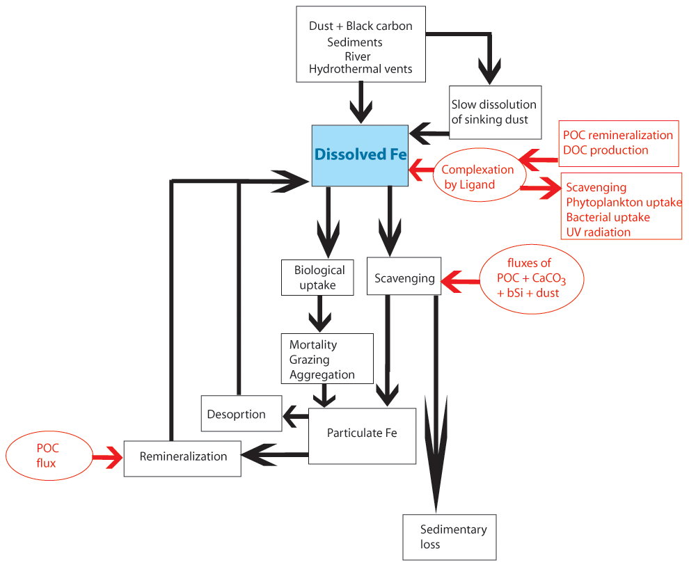
Figure 1Schematic representation of iron cycle in the ocean component of the CESM model. The texts, boxes, and arrows in black show the main processes affecting the dissolved iron pool, while those in red further show what controls the processes impacting the dissolved iron pool. POC (DOC) – particulate (dissolved) organic carbon; bSi – biogenic silica.
Iron input to the ocean is balanced by losses from biological uptake and scavenging. The biological uptake of iron is based on the species-specific Fe:C ratio, which varies based on ambient DFe concentration, as discussed previously. The biological uptake term also includes routing of phytoplankton iron to zooplankton based on its feeding preference. Losses of iron from the biological pools are through mortality, aggregation, grazing upon phytoplankton by zooplankton, and higher trophic grazing on zooplankton (Long et al., 2021). The scavenging loss of DFe is expressed as a two-step process similar to the Thorium scavenging model, involving the calculation of the net adsorption rate to sinking particles and the modification of this rate by the ambient iron concentration (Moore and Braucher, 2008). The total sinking particles consist of particulate organic carbon, biogenic silica, calcium carbonate, and dust, which strongly influence DFe scavenging in excess of ligand concentrations. The particulate organic carbon is multiplied by 6 to account for the non-carbon portion of the organic matter that can take part in scavenging. In CESM, scavenging increases non-linearly with DFe concentration. About 90 % of the scavenged iron enters the sinking particulate pool, while the rest is lost to sediments. Along with the scavenging contribution, iron released from grazing and mortality of autotrophs and zooplankton also enters the particulate iron pool. Remineralization of this sinking particulate iron replenishes DFe and is parameterized as a function of sinking particulate organic carbon flux. This results in maximum remineralization taking place within the upper 100 m, where particulate organic carbon flux is the highest. Additionally, slow desorption of sinking particulate iron also releases DFe at depths and is calculated using a constant desorption rate of 1.0 × 10⁻⁶ cm−1 for particulate iron. The model also includes an explicit ligand tracer for complexing Fe, with ligand sources being from particulate organic carbon remineralization and dissolved organic matter production. Ligand sinks involve scavenging, uptake by phytoplankton, ultraviolet radiation, and bacterial uptake or degradation (Long et al., 2021). An overview of the different sources and sinks of DFe used in CESM-MARBL is given in Fig. 1.
This study is based on five sets of simulations for identifying contributions from different sources of DFe: a control simulation (CTRL) and simulations that individually remove DFe supply from atmospheric depositions (NATM), sediments (NSED), rivers (NRIV), and hydrothermal vents (NVNT). The difference between CTRL and NATM simulations indicates the biogeochemical impacts solely due to atmospheric deposition of DFe and is referred to as the ATM case. Similarly, biogeochemical impacts solely from sedimentary, river, and hydrothermal DFe sources are, respectively, referred to as SED, RIV, and VNT cases. Simulations have been conducted in hindcast mode for 60 years using forcing from the Coordinated Ocean-ice Reference Experiments version 2 (CORE-II) dataset for the years 1948–2007 (Large and Yeager, 2009). The CORE-II data include interannual variability and consists of 6-hourly temperature, air density, specific humidity, 10 m wind speeds, and sea level pressure from the National Centers for Environmental Prediction/National Center for Atmospheric Research (NCEP/NCAR) reanalysis (Kalnay et al., 1996). Daily shortwave and longwave radiation are taken from the Goddard Institute for Space Studies-International Satellite Cloud Climatology Project radiative flux profile data (GISS-ISCCP-FD; Zhang et al., 2004). Monthly precipitation is combined with Global Precipitation Climatology Project (GPCP, Huffman et al., 1997) and Climate Prediction Center Merged Analysis of Precipitation (CMAP, Xie and Arkin, 1997) data. The monthly streamflow since 1948 used in this study has been previously derived from gauge data, where a linear regression was also employed using the CLM3 model streamflow to fill in missing data (Dai et al., 2009). The present study uses the last 10 years of simulations, given its focus on the impacts of DFe sources on the biogeochemistry of the upper 100 m of the oceans at a seasonal scale.
2.2 Observation data
Monthly climatologies for ocean temperature, salinity, and nutrients have been obtained from the World Ocean Atlas 2018 (WOA18) at 1∘ × 1∘ spatial resolution (Garcia et al., 2019). Monthly surface chlorophyll concentrations have been obtained from the European Space Agency Ocean Color Climate Change Initiative (OC-CCI) version 5 at 4 km spatial resolution for the period 2003–2020 (Sathyendranath et al., 2019). OC-CCI merges ocean color information from multiple sensors, namely the Moderate Resolution Imaging Spectroradiometer (MODIS, 2002–present), the Sea-Viewing Wide Field-of-View Sensor (SeaWiFS, 1997–2010), MEdium Resolution Imaging Spectrometer (MERIS, 2002–2012), and the Visible Infrared Imaging Radiometer (VIIRS, 2012–present). The product is bias corrected and quality controlled, yielding much lower data gaps compared to individual sensors. A monthly climatology of mixed-layer depth (MLD) gridded at 1∘ × 1∘ spatial resolution has been obtained from Argo profiles based on a hybrid algorithm that calculates a suite of MLDs using several criteria, such as gradient or threshold method, maxima or minima of a particular property, and intersection with seasonal thermocline (Holte et al., 2017). The resulting patterns are analyzed to yield final MLD estimates. To explore ocean surface circulation, Ocean Surface Current Analysis Real-time (OSCAR) data at 0.33∘ × 0.33∘ spatial resolution and 5 d temporal resolution have been used. Horizontal velocities are measured using sea surface heights, ocean surface winds, and sea surface temperatures, thereby accounting for flows due to geostrophic balance, Ekman dynamics, and thermal wind (Dohan and Maximenko, 2010).
To examine the ability of CESM to realistically simulate the variation in DFe concentrations in the upper 100 m over the northern IO, this study uses DFe profile compilations by Tagliabue et al. (2012) and the GEOTRACES Intermediate Data Product 2021 (GEOTRACES, 2021). To these, published data from Moffett et al. (2015) have also been added, comprising DFe data collected in the AS during September 2007. The DFe estimated in these data is based on the filtration of seawater through filter sizes between 0.2–0.45 µm.
First, the performance of CESM-POP2 simulations with respect to observations over the northern IO is examined. Next, the contributions of different DFe sources to upper-ocean DFe concentrations, phytoplankton blooms, and patterns of nutrient limitations are discussed. Finally, the paper explores how different sources of DFe can influence the total DFe budget across selected biophysical regimes over the northern IO.
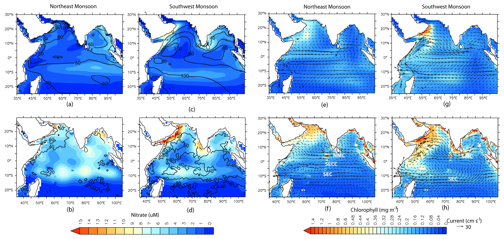
Figure 2Comparison of CESM-CTRL simulated variables (upper panels) with observations (lower panels) for the northeast monsoon (a, b, e, and f) and the southwest monsoon (c, d, g, and h). Shading in (a–d) represents nitrate concentrations averaged for upper 100 m, and the black contours are the mixed-layer depth (m). Shading in (e–h) represents surface chlorophyll concentrations, and the vectors are the surface currents. SEC – South Equatorial Current; SECC – South Equatorial Counter Current; NMC – Northeast Monsoon Current; SMC – Southwest Monsoon Current; SC – Somali Current.
3.1 Model evaluation
In this section, the CESM simulation (for CTRL case) of physical parameters, as well as of nitrate and chlorophyll concentrations, over the upper 100 m of the northern IO is evaluated. Except for MLD, ocean currents, and chlorophyll, all modeled parameters have been compared with WOA18 observations. Simulated MLDs are compared with the Argo-based values of Holte et al. (2017), ocean currents are compared with OSCAR data, and chlorophyll concentrations are compared with OC-CCI observations. In general, CESM shows good correspondence with observations of the seasonal cycle of temperature, salinity, and MLD. However, there is a positive temperature and salinity bias over IO (Figs. S2 and S3 in the Supplement). This warm bias over the IO differs from the previous version of CESM, which has a cold bias in this region (Danabasoglu et al., 2020). Figure 2 shows the seasonal climatology in CESM simulations and observations for MLD, nitrate concentrations, surface ocean currents, and chlorophyll concentrations. Overall, CESM simulates the main features of surface ocean circulation and spatiotemporal variations in MLD well. There are some deviations, such as a much stronger simulated Somali Current along the northeast coast of Africa, especially during the southwest monsoon season, which can lead to strong advection of upwelled nutrients away from this region. CESM also simulates a stronger South Equatorial Current during the southwest monsoon, which occupies a broader region compared to observations and leads to a stronger westward flow in the model between 0–5∘ S latitude. The net result of the warm and positive salinity bias is that CESM simulates a much deeper MLD than observations throughout the year across the study domain. Averaged annually, the largest overestimation (of ∼ 40 m) is over the equatorial IO, particularly during the spring and fall intermonsoon months, when the Wyrtki Jet is prevalent over the region (Fig. S3e and f in the Supplement). Additionally, MLD overestimation of ∼ 45 m is also seen over the AS during February–March and over the southern tropical IO during September–October, both associated with winter convection.
With respect to the seasonal cycle of nitrate, CESM has the least bias over the AS, followed by the BoB (Figs. 2a–d and S4 in the Supplement), but its performance is comparatively lower over the equatorial IO and southern tropical IO. For example, WOA18 data show the highest value of nitrate over the southern tropical IO in January, whereas in CESM simulations, the highest nitrate concentration is shifted to April–June in association with mixed-layer deepening. On the other hand, CESM simulates a much weaker seasonal cycle of nitrate over the equatorial IO compared to WOA18 observations. These regions over the southern tropical IO and the equatorial IO, where CESM fares poorly, also have fewer nutrient profile observations compared to the AS and BoB. For example, no more than 10 nitrate observations are available in a grid point over the southern tropical IO and equatorial IO, whereas there are several grid points over the AS, where more than 30 observations are available. Overall, CESM simulations underestimate nitrate with respect to WOA18 data for the upper 100 m of the water column.
Turning to chlorophyll concentrations, CESM simulations capture the main characteristics of the seasonal cycle and its spatial distribution over the northern IO (Figs. 2e-h and S4 in the Supplement), with certain biases and shifts in the timing of the peak blooms. For example, over the BoB, the model has difficulty in capturing the temporal evolution of chlorophyll concentrations. Over the AS and the equatorial IO, peak bloom in the simulations occurs in September in contrast to July in the observations. Similarly, over the southern tropical IO, the peak bloom is delayed in the model to October as compared to its appearance in July in observations. Most of the AS and the BoB show an underestimation (∼ −60 %) in simulated chlorophyll concentration with respect to OC-CCI values. Such an underestimation of major nutrients and chlorophyll over most of the northern IO is common to many modeling studies where coastal regimes and mesoscale processes are not adequately captured without a finer spatial resolution (e.g., Dutkiewicz et al., 2012; Ilyina et al., 2013; Long et al., 2021; J. K. Moore et al., 2013; Pham and Ito, 2021). For example, a modeling study by Resplandy et al. (2011) has shown that eddy-induced vertical transport is responsible for ∼ 40 % of nitrate fluxes in the winter convection regions of the AS during the late northeast monsoon. The study also showed that mesoscale eddies can account for 65 %–91 % of vertical and lateral advection of nitrate in the upwelling regions of the AS during the southwest monsoon. Additionally, the positive MLD bias simulated by CESM can trigger light limitation of phytoplankton growth, leading to an underestimation of chlorophyll. If the threshold depth for photosynthesis is considered to be the depth of the isolume given by 0.415 (Z0.145; Boss and Behrenfeld, 2010; Letelier et al., 2004), then the CESM-simulated MLD is deeper than the Z0.145, leading to light limitation of phytoplankton growth over the entire AS and large parts of the BoB throughout the year (Fig. S5 in the Supplement). During the southwest monsoon, almost the entire domain experiences light limitation, especially off the coast of Somalia and the southern tropical IO.
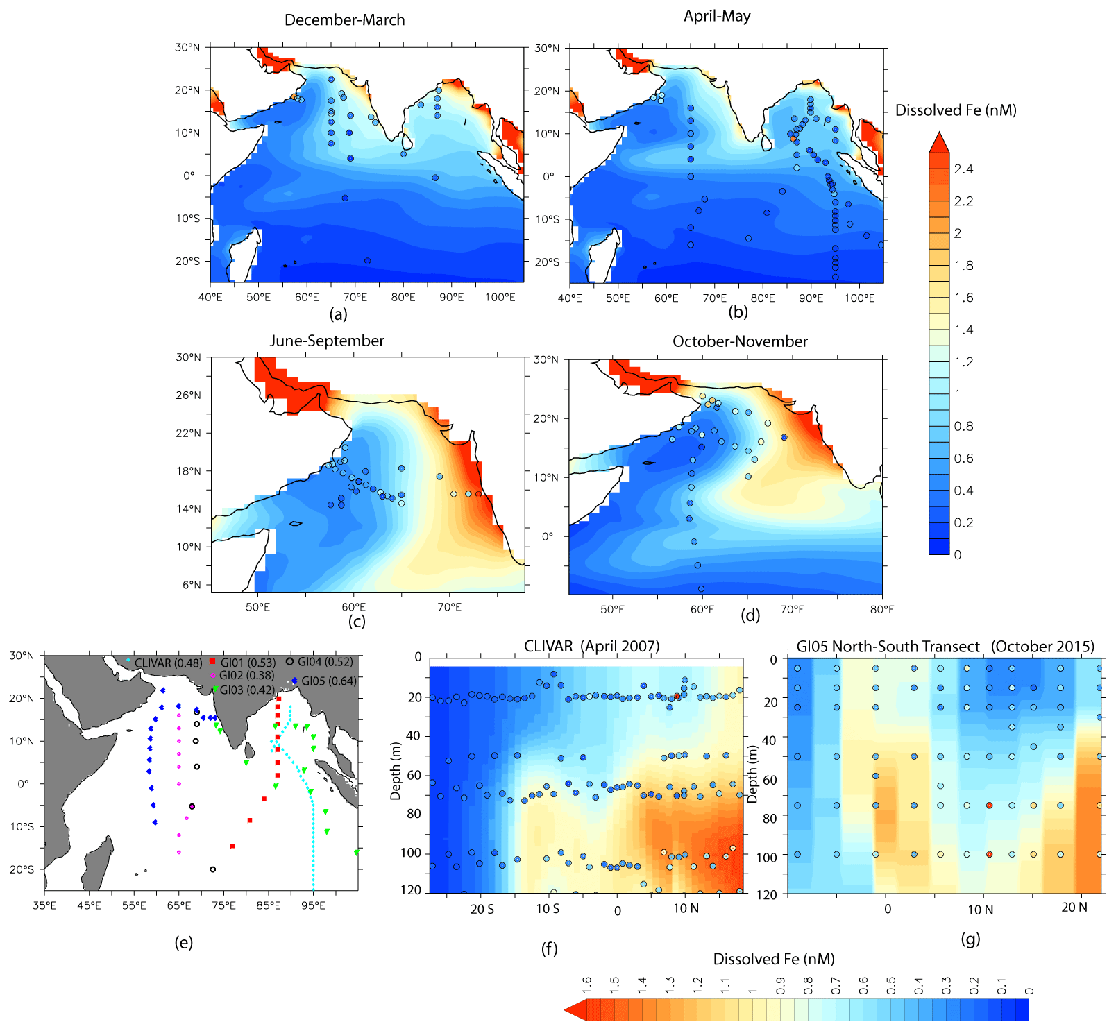
Figure 3Comparison of CESM-CTRL-simulated DFe (shading) with the observations (filled circles) compiled from various cruises. The spatial distribution maps in (a–d) consider season-wise DFe distribution averaged over the upper 20 m. (e) The different cruise tracks from which DFe measurements have been used are marked. The numbers within the parentheses are the correlation coefficients between observed and simulated DFe for each cruise. The vertical transects in (f) and (g) show DFe gradients in the water column over (f) the eastern Indian Ocean and (g) the western Indian Ocean.
CESM simulations of DFe are evaluated next using all available in situ DFe concentration data for the upper 20 m of the ocean for different seasons. In addition, the distribution of DFe along selected transects for the upper 100 m are studied: (1) CLIVAR cruise 109N along the eastern IO during April 2007 and (2) GEOTRACES cruises GI-01, GI-02, GI-03, GI-04, and GI-05. While CESM simulates the general pattern of DFe distribution over the northern IO reasonably well, DFe variation with depth and with increasing distance from the coast is stronger in simulations than in observations. For the upper 20 m, the Pearson product–moment correlation coefficient calculated between observed and simulated DFe concentrations is 0.62 (Fig. 3a–d). The coefficients for correlation between observed and simulated DFe for GEOTRACES and CLIVAR transects vary between 0.64 and 0.38 (Fig. 3e). All these correlation coefficients are significant at the 95 % confidence level based on Student's t test, with n−2 degrees of freedom, where n is the sample size. This indicates that CESM is able to reproduce the north-to-south gradient in DFe concentrations, the comparatively low DFe concentration west of 65∘ E over the AS, and the increases in DFe with depth over both the eastern and western IO reasonably well. Overall, CESM simulates a positive bias in the DFe concentration over the study domain (see Table S1 in the Supplement). A closer look at the pattern of bias in the simulated DFe reveals several features: (1) the magnitude of the positive bias is much lower to the south of 5∘ S compared to the north; (2) CESM-simulated DFe has a low magnitude of negative bias to the west of 60∘ E over the AS near the dust sources; and (3) coastal and open oceans experience similar magnitudes of positive DFe bias throughout the domain, implying that DFe bias might be stemming from multiple sources.
Figure 3f and g show two examples of the variation of DFe distribution with latitude and depth along the eastern and western IO, respectively. The model overestimates DFe values, especially to the north of the Equator and at depths greater than 60 m. Such an overestimation of DFe over the northern IO in CESM could result from a variety of factors, like source strength, assumed solubility of iron, and uncertainties in the removal of DFe by biological uptake and scavenging. With respect to source strength, dust deposition is one possible factor that can lead to the overestimation of simulated DFe. Using the Dust Indicators and Records of Terrestrial and MArine Palaeoenvironments (DIRTMAP) version 2 database of modern-day dust deposition (Kohfeld and Harrison, 2001), an attempt has been made here to understand CESM bias in dust deposition over the AS. Median dust deposition values from DIRTMAP range between ∼ 14 over the western AS (40–60∘ E), ∼ 7 over the central AS (60–70∘ E), and ∼ 20 over the eastern AS (70–80∘ E; Kohfeld and Harrison, 2001). Corresponding median values of dust deposition over these locations from the CESM model are 5, 9, and 14 , respectively, indicating a general underestimation of dust deposition by CESM, especially to the west of 60∘ E. Over the eastern IO, using mixed-layer dissolved Al concentrations, dust depositions have been estimated to be 0.2–3.0 between 20∘ S to 10∘ N (Grand et al., 2015). In a separate study, based on Al concentrations in the aerosol, Srinivas and Sarin (2013) have estimated a dust dry-deposition flux of 0.3–3.0 over the BoB. Dust deposition from the CESM is on the lower end of this range, varying from 1.1 over the northern BoB to 0.2 near the Equator. Sediment traps deployed at shallow depths over the BoB have recorded annual lithogenic fluxes that vary from the northern to the southern bay as ∼ 15 (17.5∘ N, ∼ 89.5∘ E) to ∼ 4 (5∘ N, 87∘ E; Unger et al., 2003). The corresponding variations in CESM dust deposition are ∼ 9 to ∼ 2 . Thus, overall, there is some underestimation of dust deposition over the northern IO, which might not explain the positive DFe bias in CESM simulations. However, there is a possibility of fractional solubility of Fe from dust having an impact on DFe derived from atmospheric sources. Over the AS, the percentage solubility of aerosol has been reported to vary between 0.02 % and 0.43 % (Srinivas et al., 2012). Considering that Fe constitutes 3.5 % of dust by weight and using 0.02 % and 0.5 % as the lower and upper bounds of Fe solubility, the total fluxes of soluble Fe based on CESM dust deposition are calculated. The calculated iron flux ranges from 0.002 (0.04) over the western AS to 0.01 (0.35) over the eastern AS for 0.02 % (0.5 %) solubility. The corresponding range of soluble Fe flux from CESM is 0.05 in the west to 0.8 in the eastern AS. Again, using median dust deposition values from DIRTMAP data and assuming 0.5 % iron solubility, soluble Fe fluxes vary from 0.12 to 0.17 from the western to eastern AS. It is therefore clear that the CESM model input of soluble Fe from the atmosphere is overestimated compared to observations. This inference does not change even after adding the contribution of black carbon (after assuming 6 % solubility of Fe) to the atmospheric iron flux. This is because the fractional solubility of Fe in CESM varies from 1.2 % over the northwestern AS to ∼ 5 % over the southern AS. Ship-based measurements, on the other hand, have observed that high levels of CaCO3 in the dust over the AS act as a neutralizing agent, leading to much lower aerosol solubility (Srinivas et al., 2012). Additionally, for the GI05 transect (Fig. 3g), the DFe concentration reduces drastically in the NATM case (Fig. S6a–c in the Supplement), indicating that dust deposition and its solubility are the major factors contributing to the simulated levels of DFe and its biases.
The impact of dust solubility on DFe concentration, however, does not explain the positive biases in simulated DFe over the BoB. The percentage solubility of aerosol iron measured over the BoB is high, varying between 2.3 % and 24 %, due to the presence of acid species from anthropogenic activities (Srinivas et al., 2012). This leads to much higher soluble iron deposition than what is obtained from CESM. For example, in CESM, the soluble Fe flux over BoB varies from ∼ 0.05 to 0.35 , whereas calculated soluble Fe flux varies from 0.06 to above 1 . Thus, the atmospheric supply of iron is possibly underestimated over the BoB. It is, therefore, quite possible that this positive bias in DFe stems from either sedimentary or river sources. In fact, comparing CTRL simulation with NATM and NSED along the CLIVAR transect in Fig. 3f reveals a considerable contribution of sedimentary sources of DFe, especially at depths greater than 60 m (Fig. S6d–f in the Supplement). Furthermore, the latitudinal change in salinity along this transect closely follow the latitudinal pattern of change in DFe from the NATM case but not that of DFe from the NSED case. To examine this, DFe from the NATM and NSED cases and salinity from the CTRL case have been taken along the CLIVAR transect from depths greater than 60 m and have been detrended. The correlation between DFe from NATM and salinity is −0.75, indicating that non-atmospheric sources of DFe are associated with fresher water transported from the coastal regions. The corresponding correlation between DFe from NSED and salinity is −0.16, indicating that non-sedimentary sources of DFe have no salinity dependence. The underestimation of atmospheric iron deposition and the salinity dependence of DFe from the NATM case together indicate that enhanced transport of sediments from continental margins is likely to be the source of DFe bias along the CLIVAR transect. One possible explanation is that the low resolution of the model is unable to capture the high velocity of the coastal currents that may limit the spreading of sediments from the coastal regions to the open oceans. The simulated coastal current is weaker than that of the OSCAR observations during April, when the CLIVAR measurements were undertaken (Fig. S6g and h in the Supplement). This can lead to greater diffusive spreading of iron from the coast into the open ocean. Such an effect of model resolution has been previously shown to result in a higher sedimentary contribution to DFe off the northwest Pacific and the southwest Atlantic Ocean (Harrison et al., 2018).
With respect to loss terms, biases in Fe uptake and scavenging can impact simulated DFe concentrations, especially in the surface waters. To account for Fe uptake by phytoplankton, particulate organic carbon export fluxes at 100 m, calculated from 234Th fluxes, have been used in conjunction with Fe:C ratios. Since the cellular Fe:C ratio varies widely depending on external DFe availability and phytoplankton species composition, a lower bound of 6 µmol mol−1 and an upper bound of 50 µmol mol−1 have been considered. The lower bound is based on measurements over the eastern IO (Twining et al., 2019), where oligotrophic conditions are encountered. The upper bound is based on measurements over the tropical North Atlantic, where a high dust deposition leading to high surface DFe concentrations prevails (Twining et al., 2015). Combining Fe:C values with particulate organic carbon export fluxes from JGOFS cruises (Buesseler et al., 1998) yields Fe uptake by phytoplankton that varies between ∼ 0.0004 and ∼ 0.0035 for all seasons over the AS. Phytoplankton Fe uptake from the CESM over the AS varies between ∼ 0.0001 and ∼ 0.002 , the values of which are on the lower end of observation-based values. Over the BoB, phytoplankton Fe uptake varies between ∼ 0.00002 and ∼ 0.004 based on available POC measurements (Anand et al., 2017, 2018). The corresponding range of CESM-simulated DFe uptake is ∼ 0.0002 to ∼ 0.001 , which is within the range of values calculated from observations. With respect to scavenging losses, based on the particulate Fe value from the eastern tropical South Pacific and the 234Th fluxes over the AS, Chinni and Singh (2022) estimated abiotic removal of 0.001–0.005 for the upper 100 m. In the present simulations, average scavenging removal is ∼ 0.003 over both the AS and BoB (range: 0.002 to 0.026 ) and reduces to less than 0.001 to the south of the Equator. Overall, Fe uptake by phytoplankton is possibly underestimated over the AS, which can contribute to some overestimation of DFe in the surface waters over this region. Over BoB, Fe uptake is within the range of observation-based values. Scavenging removal simulated by CESM is also within the range of observation-based values and is possibly not contributing to DFe bias in CESM.
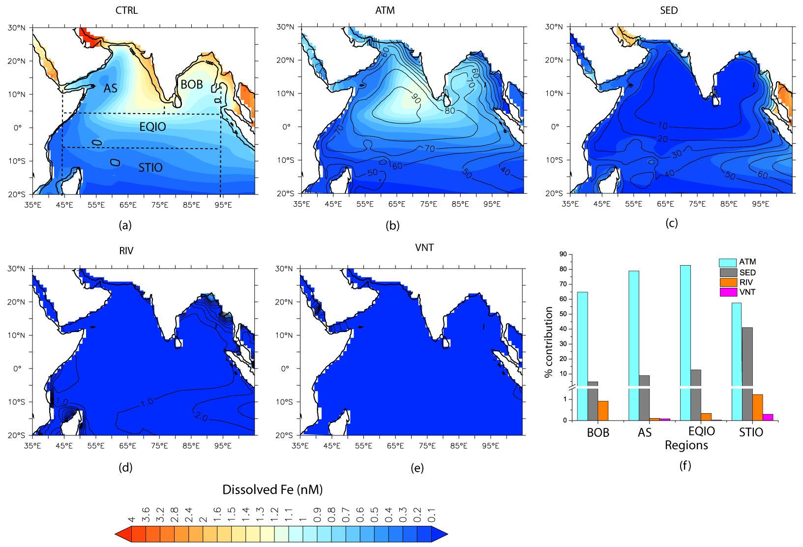
Figure 4Contribution of different sources of DFe averaged over the year to the total DFe concentrations over the upper 100 m. Shading in (a) shows the total DFe concentration with all sources included, and shading in (b–e) shows DFe concentrations arising from individual sources. Contours in (b–e) show the percentage contribution of each source to the total DFe concentrations. (f) Bar chart depicting source-specific DFe contribution (in %) over the Bay of Bengal (BoB), the Arabian Sea (AS), the equatorial IO (EQIO), and the southern tropical IO (STIO). These regions are marked by the dashed boxes in (a). The thick black contour in (a) traces the 1000 m bathymetry.
To summarize, the ocean component of CESM has a deeper MLD than observations, underestimates nitrate and chlorophyll, and overestimates DFe concentrations. Together, this can result in weaker iron limitation in the simulations compared to in the observations. Over the AS, the positive bias in simulated DFe is present mostly to the east of 60∘ E and can be related to the higher solubility of atmospheric iron in CESM compared to in the observations. Over the BoB, DFe bias likely originates from the enhanced transport of sedimentary iron from the continental shelf margins. To the west of 60∘ E, simulated DFe has a negative bias of low magnitude, possibly because the underestimation of dust deposition is counterbalanced by the overestimation of iron solubility. Over the southern tropical IO, the magnitude of bias is also low compared to the rest of the study domain. Still, the model simulates the spatial and temporal patterns of ocean physical features, as well as variations in chlorophyll concentrations, nitrate, and DFe concentrations over the northern IO, reasonably well. This gives confidence in using the model to study the iron cycle over the region. Taking the above understanding of the strengths and shortcomings of the model into account, the importance of different DFe sources with respect to the biogeochemistry of the upper 100 m of the northern IO is explored next.
3.2 Contribution of multiple iron sources
Figure 4 summarizes the contributions of different sources to the annually averaged DFe concentration. Source-wise DFe contributions for the northeast and southwest monsoons are shown in Figs. S7 and S8 in the Supplement, respectively. Overall, the relative contribution from different sources to DFe is nearly the same across different seasons, except for the somewhat higher contribution of atmospheric DFe during the southwest monsoon compared to during the northeast monsoon. This is because the arid and semi-arid regions surrounding the northern IO experience maximum dust activity from late spring to the early southwest monsoon months (e.g., Banerjee et al., 2019; Léon and Legrand, 2003). In the annual average, atmospheric deposition is the most important source of DFe over the northern IO and contributes well above 50 % of the total DFe concentrations (ATM case in Fig. 4b). Furthermore, atmospheric deposition contributes more than 70 % of the DFe supply over most of the AS, the southern BoB, and the equatorial IO. The location of the intertropical convergence zone during the northeast monsoon (∼ 10∘ S latitude) determines the southern limit of the influence of atmospheric deposition because south of the intertropical convergence zone there is a rapid reduction in DFe concentrations. Dust is the predominant contributor to the atmospheric deposition flux of iron. Over the northern AS, dust is mostly transported from Iran, Pakistan, Afghanistan, and the Arabian Peninsula, whereas over the southern AS, dust from northeastern Africa also becomes important (Jin et al., 2018; Kumar et al., 2020). Over the northern and southern BoB, the major sources of dust are the Indo-Gangetic Plain and northeast Africa, respectively (Banerjee et al., 2019). East of 90∘ E, black carbon contributes ∼ 50 % to the atmospheric DFe flux during the northeast monsoon (not shown). The source of black carbon in this region is biomass burning and fossil fuel combustion transported from the Indo-Gangetic Plain and Southeast Asia (Gustafsson et al., 2009; Moorthy and Babu, 2006).
The second largest source of DFe is from continental shelf sediments (Fig. 4c), which become dominant in the vicinity of the shelves. High sedimentary sources of DFe are characteristic of the Andaman Sea, where incoming rivers can contribute ∼ 600 × 106 T yr−1 of sediments (Robinson et al., 2007). It has been estimated that terrestrial sources contribute more than 80 % to total organic carbon in the inner shelf region of the Gulf of Martaban, adjacent to the Andaman Sea (Ramaswamy et al., 2008). Elsewhere, sedimentary contributions of ∼ 20 % to the overall DFe are found in CESM runs along the northern part of the west coast of India and the eastern BoB. Within the Ganga–Brahmaputra system, which is responsible for the discharge of ∼ 11 × 108 T yr−1 of sediments, only 10 % of sediments are estimated to be transported alongshore, with most of the sediments accumulating within the shelf and subterranean canyon (Liu et al., 2009). Over the open ocean, sedimentary sources are most important within 10–15∘ S, where the South Equatorial Current is responsible for ∼ 50 % of the DFe supply via advection from the Indonesian shelf. During the southwest monsoon, the sedimentary contribution by the South Equatorial Current extends farther westward (∼ 70∘ E; Fig. S8c in the Supplement) compared to the northeast monsoon (∼ 80∘ E; Fig. S7c in the Supplement). Signatures of elevated Al due to sedimentary contribution are seen in ship-borne measurements (Grand et al., 2015; Singh et al., 2020). In fact, such measurements have shown that the South Equatorial Current separates the DFe-rich oxygen-poor water of the northern IO from the DFe-poor oxygen-rich water of the southern tropical IO (Grand et al., 2015).
River sources contribute negligibly to total DFe concentrations (Fig. 4d), except in the immediate vicinity of the mouths of large river systems in the northeast BoB, namely the Ganges–Brahmaputra and the Irrawady–Sittang–Salween. This can arise from the fact that DFe from rivers is mostly concentrated within the fresher upper 30 m of the water column to the north of 21∘ N over the BoB and also due to high scavenging losses of iron at the river mouth. Hydrothermal vents also contribute negligibly to DFe concentrations in the upper 100 m (Fig. 4e). The hydrothermal vents supplying DFe (often in excess of 1.5 nM) in the northern IO are located in the Central Indian Ridge and the Carlsberg Ridge (Chinni and Singh, 2022; Nishioka et al., 2013; Vu and Sohrin, 2013) and largely influence DFe concentrations below 1000 m depths. The shallowest hydrothermal plumes enriched with Fe are located between ∼ 650–900 m in the Gulf of Aden (Gamo et al., 2015), overlapping with the depth range at which the Red Sea water mass spreads along the western IO (Beal et al., 2000). Since this water mass occupies progressively deeper depths with distance, sliding underneath Persian Gulf waters, surface DFe values are not impacted by these shallower vents. This is in concordance with the simulations of Tagliabue et al. (2010), where, following 500 years of model integration, hydrothermal vents increase globally averaged DFe concentrations by only ∼ 3 % in the depth range of 0–100 m.
The average contribution of different sources of iron to the upper 100 m is summarized for different open-ocean regions over the northern IO in Fig. 4f. Annually averaged atmospheric deposition is clearly the most important source of DFe throughout the northern IO. The exception to the dominant role of atmospheric deposition is the southern tropical IO, where sedimentary sources of iron contribute ∼ 40 % to the upper-ocean iron budget. Based on the analysis of origin of bias in simulated DFe concentrations in Sect. 3.1, it is likely that the contribution of atmospheric sources to the upper-100 m DFe concentration is overestimated over the eastern AS and that the contribution of sedimentary sources to the upper-100 m DFe concentration is overestimated over the BoB. Averaging over the entire domain, the atmospheric source contributes ∼ 67 % to the upper-100 m DFe concentration. On masking out the region to the east of 65∘ E over the AS, where the highest positive bias of DFe from dust has been noted, it is seen that the atmospheric source contributes ∼ 65 % to the upper-100 m DFe concentration. Again, averaging over the study domain, the sedimentary source contributes ∼ 30 % to the upper-100 m DFe concentration. On masking out the BoB, where a positive bias of DFe from sedimentary sources has been identified in Sect. 3.1, it is seen that the sedimentary source contributes ∼ 33 % to the upper-100 m DFe concentration. Thus, while biases in the source strength might regionally impact the percentage contribution of DFe from various sources to the northern IO, the overall conclusion of atmospheric source being the most important for upper-ocean DFe over the northern IO, followed by sedimentary sources, does not change. The river contribution is generally ∼ 1 %, with slightly higher contributions in the BoB and the southern tropical IO. Hydrothermal vents make negligible contributions throughout the northern IO. Adding these four sources of DFe estimated from CESM experiments does not yield the full 100 % of the DFe source, owing to non-linear effects associated with iron removal processes and complexation by organic ligands.
3.3 Phytoplankton responses to multiple iron sources
In this section, the impact of different sources of DFe on phytoplankton growth is examined. Since river and hydrothermal sources make negligible contributions to the upper-ocean iron concentrations, as shown above, these are not considered further.
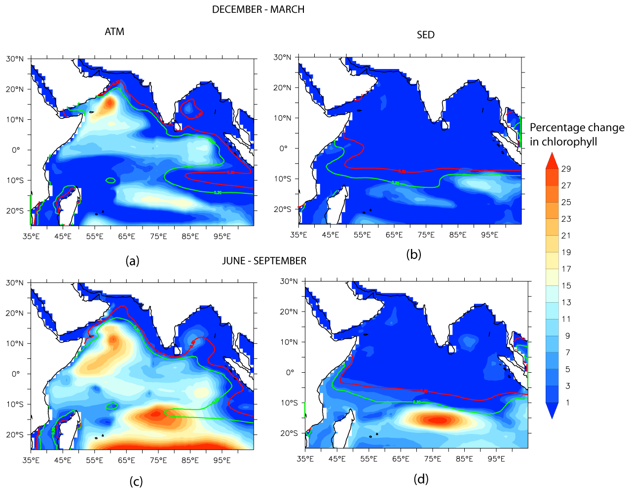
Figure 5Percentage contribution of (a) and (c) atmospheric and (b) and (d) sedimentary sources of iron during (a) and (b) the northeast monsoon and (c) and (d) the southwest monsoon to the upper 100 m chlorophyll concentrations. Green and red contours show background DFe concentrations of 0.2 and 0.3 nM, respectively. For the ATM (SED) case, background DFe is obtained from the NATM (NSED) simulation.
3.3.1 Responses to atmospheric depositions
During the northeast and southwest monsoons, atmospheric DFe brings about increases in column-integrated chlorophyll concentrations over most of the northern IO (Fig. 5a and c). The largest column-integrated positive response is seen in the western AS (west of ∼ 65∘ E) throughout the year, where atmospheric DFe accounts for more than ∼ 20 % of the column-integrated chlorophyll concentration and more than 50 % of the surface chlorophyll concentration (Fig. S9 in the Supplement). This region comes under the influence of upwelling during the southwest monsoon and mixed-layer deepening due to winter convection during the northeast monsoon, which can supply the macronutrients required for phytoplankton growth (Madhupratap et al., 1996; Morrison et al., 1998). The other region displaying a strong positive response is the southern tropical IO during June–September, where atmospheric DFe contributes ∼ 20 % (∼ 35 %) of the column (surface) chlorophyll concentration. This is the time of the year when a deep mixed layer leads to the entrainment of nutrients into the surface layers (Końe et al., 2009; Lévy et al., 2007). In contrast, there are some regions, like the northern and western AS, the west coast of India, and large parts of the BoB and the eastern IO, which, in spite of receiving high atmospheric DFe, hardly experience any chlorophyll response. These regions show < 1 % increase in column chlorophyll concentrations and generally coincide with high sedimentary iron input. This is discussed further in Sect. 3.3.3
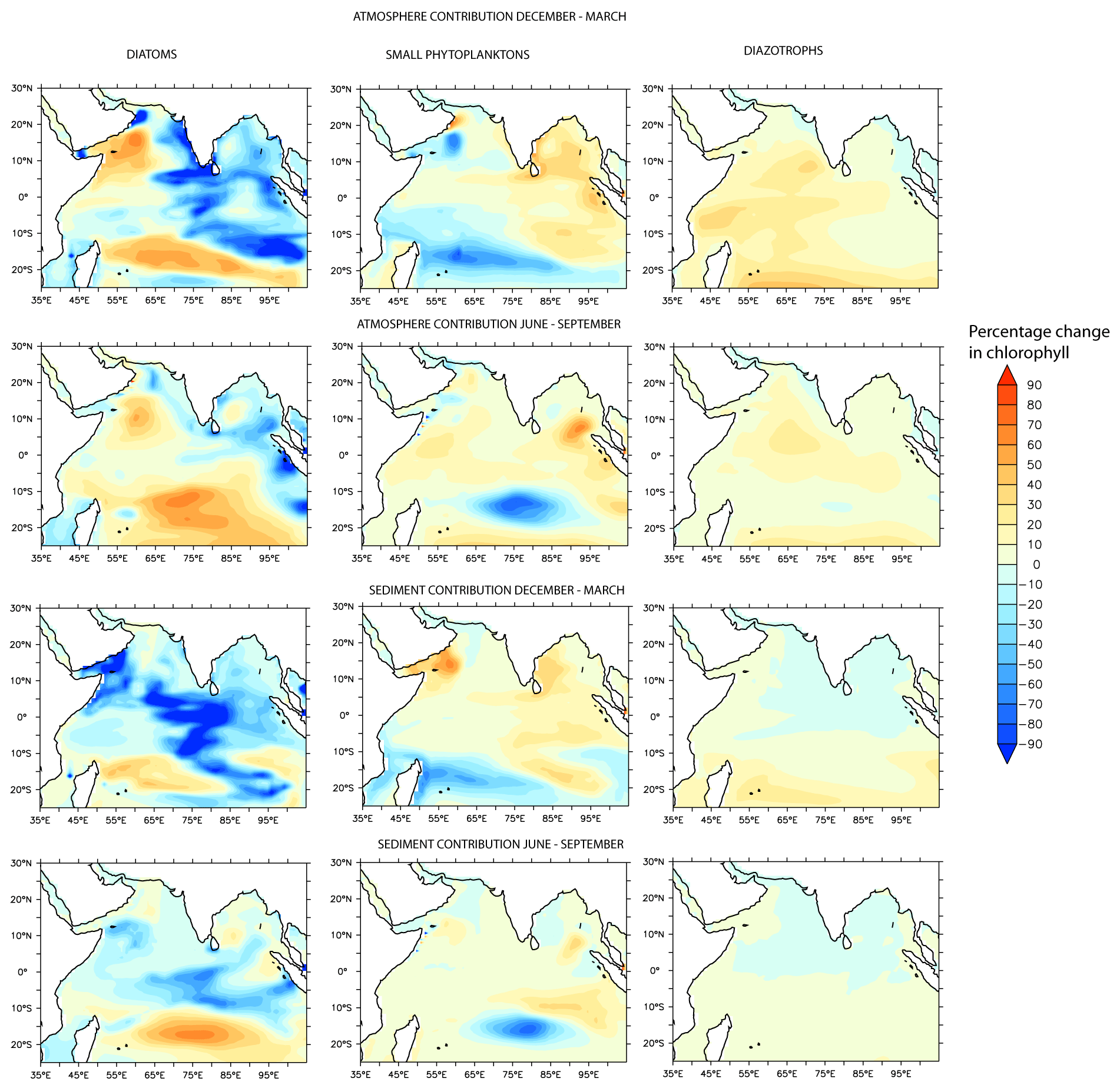
Figure 6Species-wise percentage contribution to column chlorophyll (0–100 m) response associated with atmospheric and sedimentary sources of DFe.
Species-wise decomposition shows that the increases in chlorophyll during both the northeast and southwest monsoons are driven by increases in diatoms and declines in small phytoplankton (Fig. 6). For example, over the western AS and southern tropical IO, diatoms increase by at least 40 %, and small phytoplankton populations decline by at least 50 %. An exception is the equatorial IO, where the positive response of chlorophyll arises from the growth of small phytoplankton. In general, this region has very low levels of macronutrients and is dominated by picoplankton (Vidya et al., 2013). Those regions exhibiting < 1 % increase in phytoplankton in response to atmospheric DFe, in contrast, are characterized by the proliferation of small phytoplankton and reductions of diatoms. Although diazotrophs show a positive response to the atmospheric DFe addition throughout the region, this group constitutes only ∼ 1 % of the total phytoplankton biomass.
Such differences in species response to external iron addition arise from differences in nutrient uptake between different phytoplankton functional groups in CESM. The phytoplankton growth rate (μi) is parameterized as a product of resource-unlimited growth rate (μref in d−1) at a reference temperature of 30 ∘C and three terms that describe nutrient limitation (Vi), temperature dependence (Tf), and light availability (Li). This is expressed as follows:
The nutrient limitation term for iron, Vi, for a specific phytoplankton group i is expressed as follows:
where Fe is the concentration of iron, and is the Fe uptake half-saturation constant for a phytoplankton group. While small phytoplankton have been assigned a value of 3.0 × 10⁻⁵ mmol m−3 for , diatoms have been assigned a higher value of 7.0 × 10⁻⁵ mmol m−3. This leads to the small phytoplankton outcompeting diatoms when nutrient levels are low. Additionally, small phytoplankton are subjected to higher grazing pressure than diatoms. The maximum grazing rate assigned in CESM is 3.3 d−1 for small phytoplankton versus 3.15 d−1 for diatoms. Together, the differences in the nutrient uptake half-saturation constant and the grazing pressure between different phytoplankton species result in diatom-dominating blooms under nutrient-replete conditions.
Diatoms outperforming other phytoplankton species has been previously witnessed in in situ iron fertilization experiments along with the existence of a linear relationship between diatom size and iron requirement for growth (de Baar et al., 2005). Such shifts in phytoplankton community structure in response to DFe additions are also corroborated by in situ experiments over the northern IO. For example, a nutrient addition experiment over the northern AS during the northeast monsoon period has shown that the maximum positive phytoplankton response takes place due to nitrate + DFe addition (instead of only DFe addition), accompanied by around 4-fold increases in coccolithophores, pennate, and large centric diatoms (Takeda et al., 1995). Ship-board iron addition experiments over the AS during the southwest monsoon resulted in the proliferation of visible colonies of the haptophyte Phaeocystis sp. due to silicate limitation (Moffett et al., 2015). Over the eastern IO, where both macronutrients and micronutrients are low, nutrient spiking with nitrogen, phosphorus, and iron resulted in an increase of Prochlorococcus, Synechococcus, and Eukaryotes (Twining et al., 2019).
3.3.2 Responses to sedimentary sources of iron
As shown in Fig. 4, sedimentary sources supply less than ∼ 20 % of DFe north of ∼ 10∘ S, whereas between 10–15∘ S, sedimentary iron can contribute to almost half of the total DFe concentrations. Unlike atmospheric sources, the sedimentary supply of DFe is mostly confined to regions adjoining continental shelves and islands, from where they are introduced to the open ocean by seasonally varying currents. In general, sedimentary sources make a modest contribution to column productivity (< 1 % of chlorophyll anomalies) to the north of ∼ 10∘ S, as described above. This is because high dust deposition to the north of the intertropical convergence zone results in high background DFe concentrations and controls productivity (see also Sect. 3.3.3). Sedimentary sources trigger the strongest positive phytoplankton response over the southern tropical IO region during June–September, where sedimentary DFe advected by the South Equatorial Current can facilitate an increase of more than 20 % of the upper-100 m chlorophyll concentrations and an increase of ∼ 40 % at the surface. As noted in Sect. 3.2, although atmospheric deposition contributes nearly half of the total DFe addition to this region, the total iron deposition here is low (< 0.2 nM). The phytoplankton response over the southern tropical IO is dominated by an increase in diatoms, which contribute to more than 60 % of total phytoplankton biomass (Fig. 6). In contrast, over the regions experiencing < 1 % chlorophyll increase, there is a shift from diatoms towards small phytoplankton species (Fig. 6). For example, there is a reduction of more than 80 % in diatoms and an increase of 50 % in small phytoplankton over the western AS. Other current systems such as the poleward-flowing Somali Current, the eastward-flowing Southwest Monsoon Current, and its southward extension along the west coast of Indonesia also transport sedimentary DFe to the open ocean, but such advection supports only ∼ 5 % phytoplankton biomass.
It is important to mention here that DFe bias arising from source strength has a low impact on phytoplankton response to a particular source of DFe. This is because the strongest phytoplankton response to a specific DFe source is over the western AS and subtropical southern IO. As noted in Sect. 3.1, these regions have the lowest magnitude of DFe bias. For example, averaging over the upper 100 m over the northern IO, atmospheric sources contribute ∼ 13 % to the total chlorophyll concentration. Even after masking out the region to the east of 65∘ E over the AS, where the highest positive DFe bias arising from atmospheric Fe has been noted, it is seen that atmospheric sources contribute ∼ 13 % to the upper-100 m chlorophyll concentration. Similarly, sedimentary sources contribute ∼ 9 % to the upper-100 m chlorophyll concentration over the entire northern IO domain. Masking out the BoB, where DFe bias is due to enhanced sediment transport, results in sedimentary sources contributing ∼ 8 % to the upper-ocean chlorophyll concentration.
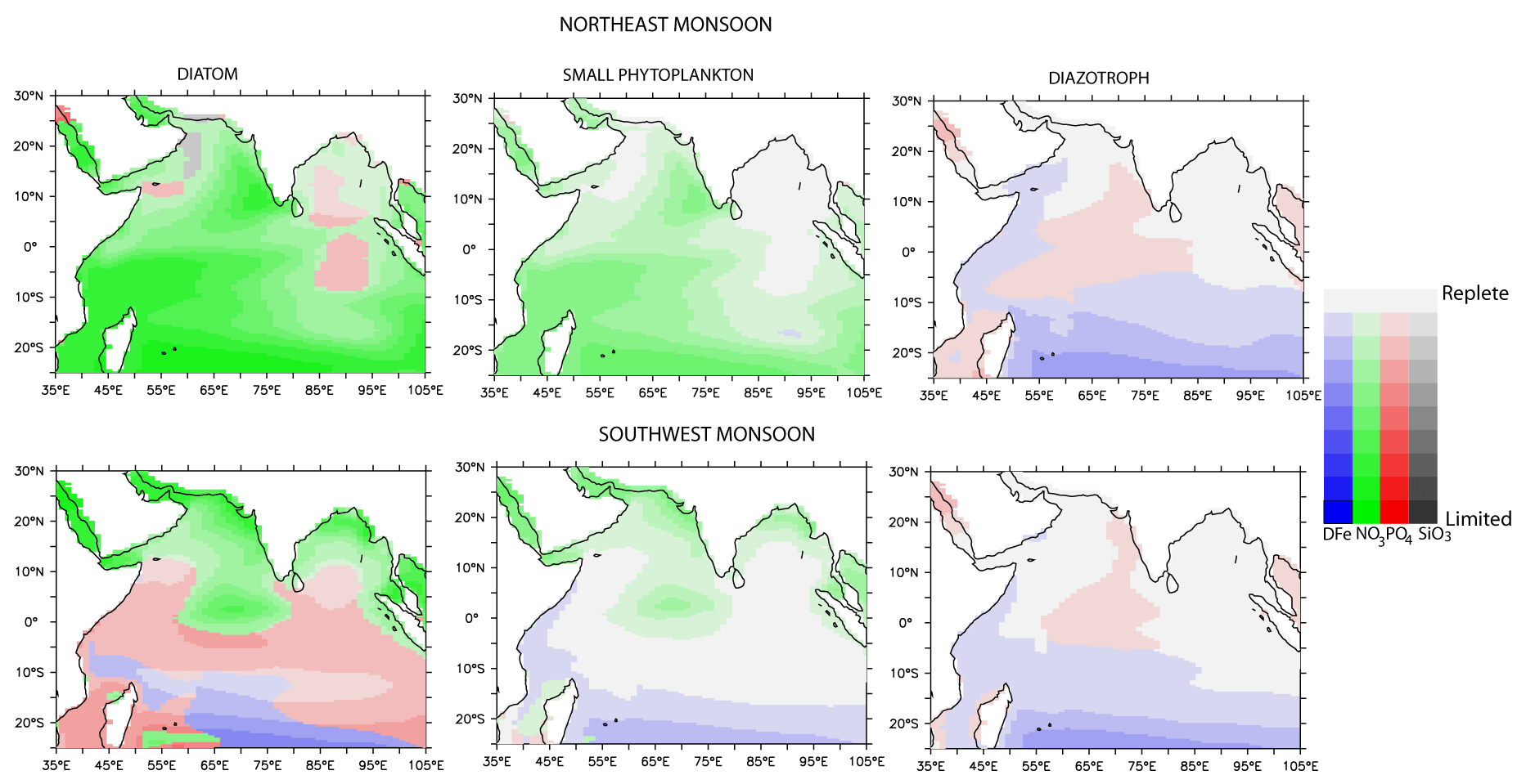
Figure 7Patterns of surface nutrient limitations for different phytoplankton functional types from the CTRL simulation. Green – nitrate; blue – iron; red – phosphate; gray – silicate limitations.
3.3.3 Role of background nutrients in phytoplankton responses to external iron
It emerges from the previous sections that there is heterogeneity in the phytoplankton response to atmospheric and sedimentary sources of DFe. The regions receiving the highest DFe input from a specific source are not always the regions where the strongest phytoplankton responses are evoked. What explains these differing patterns of phytoplankton response? To examine this, patterns of nutrient limitations and iron supply from an external source with respect to background DFe and nitrate (NO3) concentrations are examined. In considering the phytoplankton response to atmospheric sources (ATM case), background DFe is taken from the simulation without any atmospheric source (NATM). Since river and hydrothermal sources make negligible contributions to DFe over this domain, high levels of DFe in NATM mainly arise in regions where sedimentary sources are important. Similarly, for estimating phytoplankton response to sedimentary sources (SED case), the background DFe is taken from the simulation without any sedimentary source (NSED).
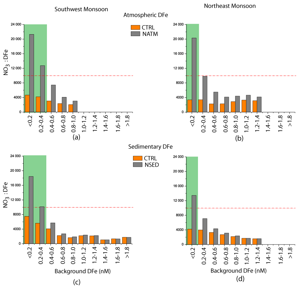
Figure 8Relation between background nutrients and phytoplankton response for atmospheric (a) and (b) and sedimentary (c) and (d) sources of DFe during (a) and (c) the southwest monsoon and (b) and (d) the northeast monsoon. The horizontal axis shows background DFe concentrations. The orange columns show the upper-ocean NO3:DFe ratio for the CTRL case, and the gray columns show the NO3:DFe ratio for the (a–b) NATM and (c–d) NSED cases. The dashed red lines show the location where the NO3:DFe ratio is 10 000; below this value, N limitation prevails in CESM. Green shades highlight the regions where > 1 % increase in chlorophyll following DFe addition from a specific source is induced.
Generally, those regions experiencing > 1 % increase in chlorophyll in response to atmospheric (sedimentary) sources coincide with background DFe concentrations of < 0.2–0.3 nM and high background NO3:DFe ratios from the NATM (NSED) simulation. For example, in the NATM simulation, iron serves as the dominant nutrient that limits productivity over the entire northern IO, with diatoms experiencing stronger iron limitation compared to other phytoplankton groups (Fig. S10 in the Supplement). Iron limitation is particularly severe over the central and southern AS, the equatorial IO, and the southern tropical IO. In the NSED case, there is a switch from nitrate limitation to the north of the intertropical convergence zone to iron limitation to the south of the intertropical convergence zone (Fig. S11 in the Supplement). While iron stress is alleviated with the addition of external DFe, there is a shift towards macronutrient, especially nitrate, limitation (Fig. 7). The region south of ∼ 15∘ S continues to experience iron limitation during June–September due to very low dust deposition. In contrast, regions where the chlorophyll increase is < 1 % following DFe addition are characterized by nitrate limitation in the NATM and NSED simulations, and external DFe cannot alleviate this primary nutrient limitation. This is further illustrated in Fig. 8, where the upper-ocean NO3:DFe ratio is plotted against the background DFe concentrations. A positive chlorophyll response is elicited in regions of the lowest background DFe and the highest background NO3:DFe ratio. Over the world oceans, a wide range of cellular Fe:C ratios has been observed for diatoms, ranging from 100 µmol mol−1 for DFe-replete conditions (Twining et al., 2015, 2021) to 2 µmol mol−1 for DFe-deplete conditions (de Baar et al., 2008). Assuming a C:N ratio of 117:16 (Anderson and Sarmiento, 1994), the ranges of N:Fe ratios obtained are ∼ 1000 and ∼ 68 000, respectively, for DFe-replete and DFe-deplete conditions. Similarly, by considering the iron limitation that takes place for the Fe:C ratio of 10 µmol mol−1 for open-ocean species based on laboratory experiments (Sunda and Huntsman, 1995) and the C:N ratio of 106:16, Measures and Vink (1999) have estimated that iron limitation over the AS water takes place at a NO3:DFe ratio greater than ∼ 15000. In CESM simulations, > 1 % increase in chlorophyll takes place when the initial upper-ocean NO3:DFe ratio is more than 10 000, corresponding to Fe limitation scenario (Fig. 8). With the addition of DFe from atmospheric or sedimentary sources, the upper-ocean NO3:DFe ratio reduces to less than 4000 in some cases, thereby leading to N limitation. Previously, iron addition experiments in the AS during the southwest monsoon have shown that the positive chlorophyll response depends on initial nitrate concentrations, with this response increasing in magnitude with higher initial nitrate concentrations (Moffett et al., 2015). In summary, the initial upper-ocean NO3:DFe ratio sets the ultimate limit to the magnitude and distribution of phytoplankton response following external DFe additions.
To sum up, atmospheric deposition is the most important source of DFe to the upper 100 m over the entire northern IO, followed by sedimentary sources. While atmospheric DFe is deposited over wide areas of the open ocean, sedimentary DFe fluxes arise only from continental shelves and are transported to open oceans through advection by currents. River and hydrothermal sources make negligible contributions to the total iron budget in the upper 100 m. The primary response to atmospheric DFe is an increase in column-integrated phytoplankton biomass over most of the northern IO. In contrast, the sedimentary source of iron is responsible for increases in column-integrated phytoplankton biomass, mainly to the south of the intertropical convergence zone, where dust depositions are low. In general, significant positive responses of phytoplankton to the addition of DFe are simulated only where low levels of background DFe concentrations and high values of the background NO3:DFe ratio are present. Otherwise, nitrate becomes the limiting nutrient once DFe is added. The simulations also show that a positive chlorophyll response to addition of DFe generally involves the proliferation of diatoms, except over the equatorial IO, where a small phytoplankton increase is seen.
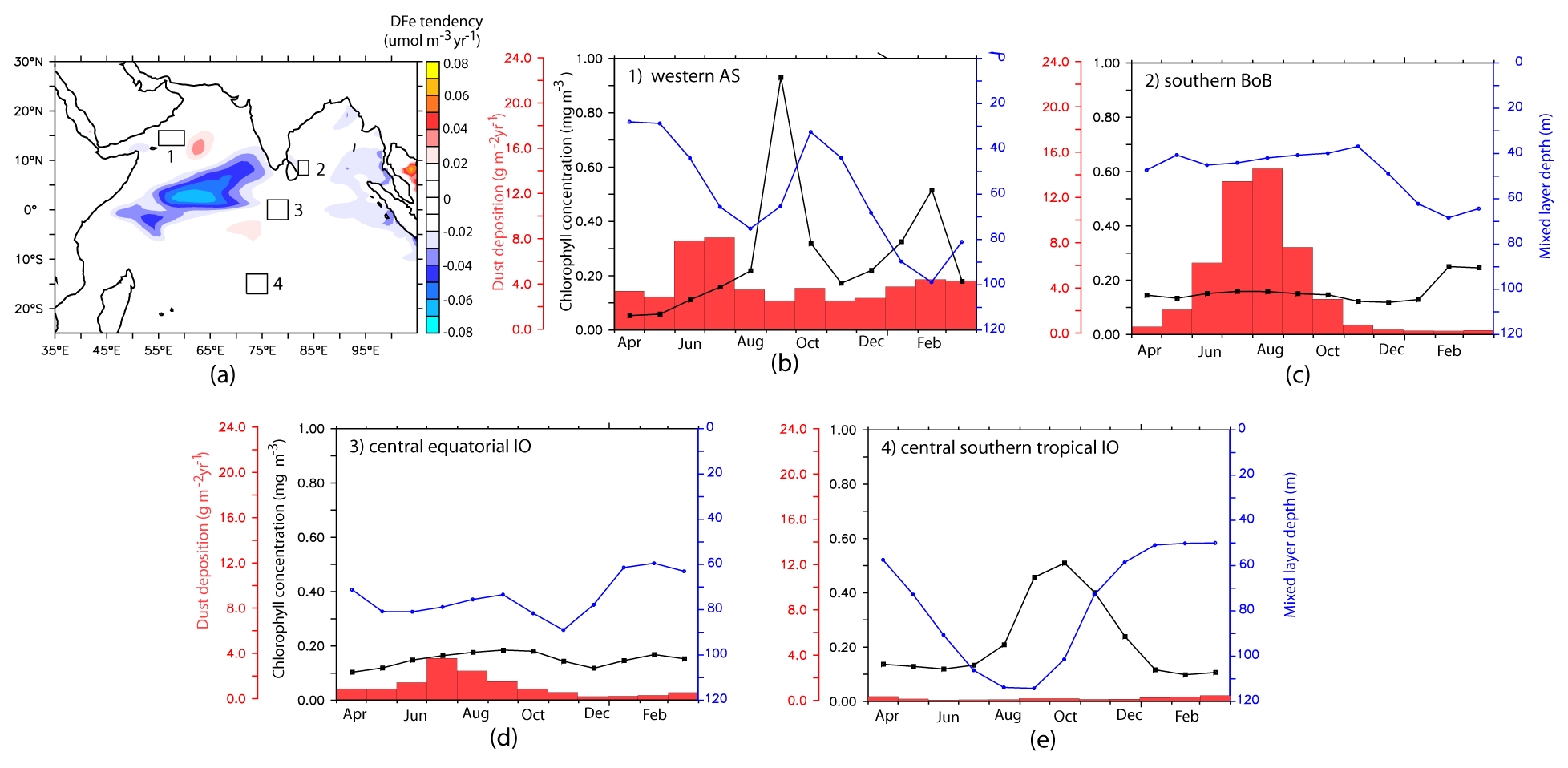
Figure 9(a) Net DFe tendency averaged over the upper 100 m for the study period. The boxes indicate the regions chosen for further studying the DFe budget in Sect. 3.4. (b–e) Seasonal cycle of dust deposition (red columns), mixed-layer depth (blue curves), and chlorophyll concentrations (black curves) from CESM-CTRL case for the four regions marked in (a).
3.4 Iron budgets across different biophysical regimes
This section explores the main processes controlling the DFe budget with respect to the role of atmospheric and sedimentary sources over different biophysical regimes of the northern IO, namely (1) the western AS, (2) the southern BoB, (3) the central equatorial IO, and (4) the central southern tropical IO. These regions encompass a wide range of productivity, with the first region being highly productive, with OC-CCI chlorophyll exceeding 1.5 mg m−3. The southern BoB and central southern tropical IO are moderately productive. Lastly, the central equatorial IO is oligotrophic, with the surface chlorophyll concentration being ∼ 0.1 mg m−3. The locations of these regions, along with CESM-simulated seasonal cycles of mixed-layer depths, chlorophyll, and dust depositions, are shown in Fig. 9.
The net dissolved-iron tendency (TENDDFe) is calculated as follows:
where the source terms on the right describe dust, sediments, rivers, or vents (EXT); horizontal and vertical advection (ADV); horizontal and vertical mixing (MIX); and biological sources or sinks (BIO). Advection includes explicitly resolved velocity and an additional bolus velocity from the parameterization of mesoscale eddies (Gent and McWilliams, 1990). Vertical mixing includes a tracer-gradient-dependent term for cross-isopycnal mixing and a non-local mixing term, which accounts for mixing due to convective and shear instabilities (Large et al., 1994). Lateral mixing involves the parameterization of mesoscale eddy-induced horizontal diffusion along isopycnal surfaces (Redi, 1982). The BIO term includes DFe losses due to biological iron uptake and scavenging, recycling of iron back to the pool via remineralization, and iron released from phytoplankton and zooplankton losses and grazing.
3.4.1 Western Arabian Sea
The western AS, off the Oman and Yemen coastlines (considered here to be 13–16∘ N and 55–60∘ E), is the most productive region in the northern IO. Primary productivity in the western AS is highest during the southwest monsoon (Fig. 9b), during which alongshore southwesterly winds lead to upwelling and bring subsurface nutrients from depths of ∼ 150–200 m (Morrison et al., 1998). Some of this upwelled water advects eastwards, transporting nutrients that enhance productivity in the central AS (Prasanna Kumar et al., 2001). The region also experiences a secondary bloom during the northeast monsoon due to winter convection that deepens the mixed layer. Integrated over depths of the euphotic zone, the average primary productivity over the western AS during the middle and late southwest monsoon is estimated at 135 ± 10 and 110 ± 11 , respectively (Barber et al., 2001). In comparison, primary productivity over the western AS during the middle and late northeast monsoon is 137 ± 13 and 88 ± 4 (Barber et al., 2001). Although this region encounters high dust deposition (Haake et al., 1993; Mahowald et al., 2009), in situ measurements have hypothesized possible iron limitation during the late southwest monsoon because upwelled water is drawn from above the iron-rich sub-oxic zone (Naqvi et al., 2010).
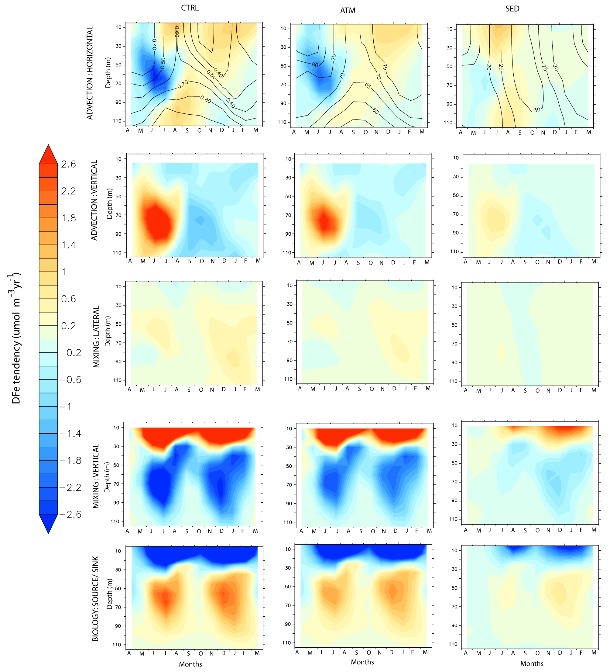
Figure 10Evolution of the various terms of the DFe budget, expressed as , by month and depth over the western Arabian Sea. Left panels: CTRL; middle panels: ATM; right panels: SED case. The contours in the upper panel for the CTRL show the evolution of DFe concentrations (nM), while the contours in the upper panels for the ATM and SED cases show the percentage contribution of each of these cases to the total DFe concentrations in the CTRL case.
The largest peak in dust deposition is during the southwest monsoon, followed by a second peak during the northeast monsoon (Fig. 9b). Accordingly, the upper-ocean DFe concentration is highest during the southwest monsoon and is dominated by atmospheric sources (Fig. 10). The sedimentary contribution, although much lower, peaks during the late southwest monsoon and fall intermonsoon months. Throughout the year, the DFe concentration increases with depth, thus pointing to consumption by phytoplankton at the surface. Vertical advection and vertical mixing are the most important physical mechanisms governing DFe supply within this region during the southwest monsoon (Fig. 10). These processes begin to strengthen from May onwards, reaching their peak during June–July and decreasing thereafter. Decomposing the DFe advection tendency into tendencies arising from gradients in the tracer distribution (DFe′) and velocity convergence (U′), respectively, it is seen that vertical advection of DFe arises from DFe′ and U′ in equal magnitude. However, the former process is dominant in June, and the latter process dominates during July (Fig. S12 in the Supplement). The maximum vertical advection of DFe is centered around 80 m depth and progressively reduces at shallower depths as the vertical velocity reduces towards the surface. Vertical mixing prevailing in the upper 40 m brings this vertically advected DFe from the subsurface to the surface. Furthermore, horizontal advection plays an important role in redistributing this DFe supplied by vertical processes, with contributions from horizontal U′ being at least twice as large as DFe′ . During the spring and early southwest monsoon, northeastward horizontal advection removes atmospheric deposited DFe throughout the upper 100 m while aiding the supply of sedimentary DFe from the Somalia and Omani continental shelves to the western AS. Later in the year, as the southwest monsoon current circulation is established and meridional currents along the western AS become stronger, its effect is first evident in the south along the Somali coast and progresses northward with time. The result is the convergence of both atmospheric and sedimentary DFe in the western AS during July–September. During the northeast monsoon, vertical mixing driven by winter convection, with the mixed-layer deepening to 100 m, is the most important means of DFe supply from both atmospheric and sedimentary sources into the surface layer. Additionally, horizontal advection by westward currents transports DFe from atmospheric deposition in the central AS into the western AS.
The removal of DFe from the water column is mainly through biological uptake in the upper 40 m. Uptake of DFe by small phytoplankton dominates biological uptake throughout the year, except during September–October, when uptake of DFe by diatoms becomes significant (not shown). This signature of diatoms is also observed in opal fluxes measured by sedimentary traps deployed near the western AS and has been attributed to the lowering of zooplankton grazing pressures during the late southwest monsoon (Smith, 2001) and to the silicate limitation of diatoms in initially upwelled waters (Haake et al., 1993). In the subsurface layer, remineralization of sinking fluxes of particulate iron peaking at ∼ 50 m replenishes the DFe pool during the latter part of the productive months (Fig. S16a in the Supplement). Iron so released is made available to the surface layer via mixing or advection, thereby playing an important role in maintaining the surface DFe pool. Some of the remineralized DFe is further removed by scavenging, which peaks at ∼ 80 m during the productive months due to large fluxes of sinking particulate organic carbon, biogenic silica, calcium carbonate, and dust (Fig. S16a in the Supplement). Atmospheric deposition dominates the biological source or sink of DFe throughout the year, while sedimentary DFe is more important for biology during the northeast monsoon months.
3.4.2 Southern Bay of Bengal
The region corresponding to the southern BoB (7–10∘ N and 82–84∘ E) is located to the east of Sri Lanka. Compared to the rest of the BoB, freshwater flux from South Asian rivers reduces markedly in this region due to the advection of high-salinity water from the AS by the eastward-flowing Southwest Monsoon Current (see Fig. 2h) and the upward pumping of saltier water by thermocline doming during the southwest monsoon season (Vinayachandran et al., 2013). This leads to stronger biophysical coupling in the southern BoB compared to the rest of the bay through the erosion of the upper stable layer of freshwater capping. During the southwest monsoon, the Southwest Monsoon Current advects nutrients and chlorophyll from the upwelling regions along the southern tip of India and Sri Lanka into the southern BoB (Vinayachandran et al., 2004). Over the open southern BoB, to the east of Sri Lanka, the cyclonic wind stress curl drives open-ocean upwelling, leading to shoaling of the thermocline that forms the Sri Lankan dome. This results in surface chlorophyll concentrations between 0.3–0.7 mg m−3 and strong subsurface chlorophyll maxima between 20–50 m where the chlorophyll concentration can exceed 1 mg m−3 (Thushara et al., 2019). A much lower magnitude of surface chlorophyll concentration (∼ 0.18 mg m−3; Fig. 9c) and subsurface chlorophyll maxima (∼ 0.2 mg m−3) at 40–60 m depth is simulated by CESM. During the northeast monsoon, CESM simulates a second bloom over this region associated with winter cooling and mixed-layer deepening to ∼ 60 m (Fig. 9c). This bloom has a slightly higher magnitude, peaking at ∼ 0.25 mg m−3, compared to the southwest-monsoon bloom. Surface chlorophyll data from OC-CCI also reveal the presence of northeast-monsoon blooms (peak at ∼ 0.25 mg m−3), which, during some years, are of higher magnitude than southwest-monsoon blooms. Argo data in this region also show signatures of mixed-layer deepening during winter (not shown).
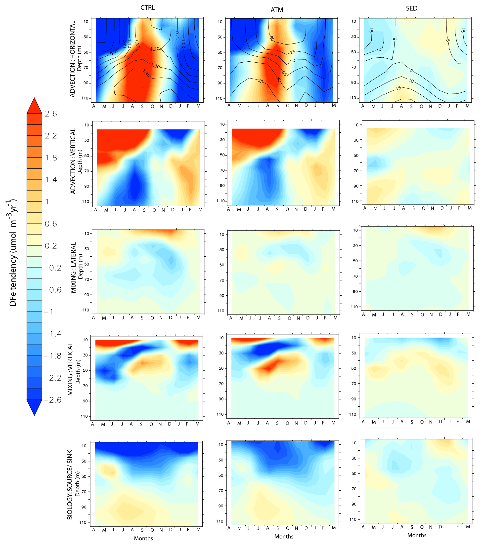
Overall, the highest DFe over this region is encountered during the late southwest monsoon and is dominated by atmospheric deposition (Fig. 11). Vertical advection is the most important process supplying DFe to the surface layers during the spring and southwest monsoon months (Fig. 11). This is aided by a positive wind stress curl established over the region from March onwards. While vertical velocity is positive during the southwest monsoon over the entire depth considered, DFe supply by vertical advection is positive only for depths less than 50 m (Fig. S13 in the Supplement). This is because the magnitude of upward velocity gradually reduces with depth, resulting in positive values of U′ upwards from 40 m depths. (Fig. S13 in the Supplement). With the arrival of westward-propagating Rossby waves to the western boundary of the BoB during October, upwelling-favorable vertical motion collapses (Webber et al., 2018).
With respect to horizontal advection, it is seen that the magnitude and sign of convergence by the meridional component of the current mainly control DFe supply over the southern BoB. This arises from the southward-flowing current to the western flank of the Sri Lankan dome that supplies atmospheric DFe to this region. This DFe supplied by the southwards current, as well as the DFe derived from upwelling, is removed by the energetic eastward currents during the late-spring to early-fall intermonsoon months. During the rest of the year, the westward-flowing currents supply some sedimentary DFe from the Andaman Sea to the southern BoB. However, the much-larger magnitude of dust deposition in the northwestern BoB leads to overall negative tracer gradients and, thus, dilution of DFe by horizontal advection. The most important DFe supply mechanism during the northeast monsoon is enhanced vertical mixing in the upper 20 m associated with deepening of the mixed layer. Additionally, downwelling due to weakly negative wind stress curl during this time of the year removes DFe from the surface and favors its accumulation in the subsurface ocean. Lateral mixing complements DFe supply to the upper 20 m during the fall and early northeast monsoon, especially from sedimentary sources.
Biological uptake removes DFe throughout the year from the upper 40 m, especially during the southwest- and northeast-monsoon blooms (Fig. 11). DFe uptake in the upper 40 m is dominated by small phytoplankton during most of the year, except during the northeast monsoon (not shown). Diatom DFe uptake, on the other hand, dominates the deep chlorophyll maxima present between 40–70 m throughout the year and within the surface layer during the northeast monsoon months. Several studies have pointed to substantial nutrient uptake by diatoms in the central, coastal, and northern BoB due to riverine supply of silicates (Madhu et al., 2006; Madhupratap et al., 2003). Remineralization of particulate iron, as well as iron release from grazing and mortality of phytoplankton and zooplankton, has a primary peak between 50–80 m during July–August and a secondary peak during February–March. On the contrary, scavenging removes DFe, with its effect peaking during July–August during blooms (Fig. S16b in the Supplement).
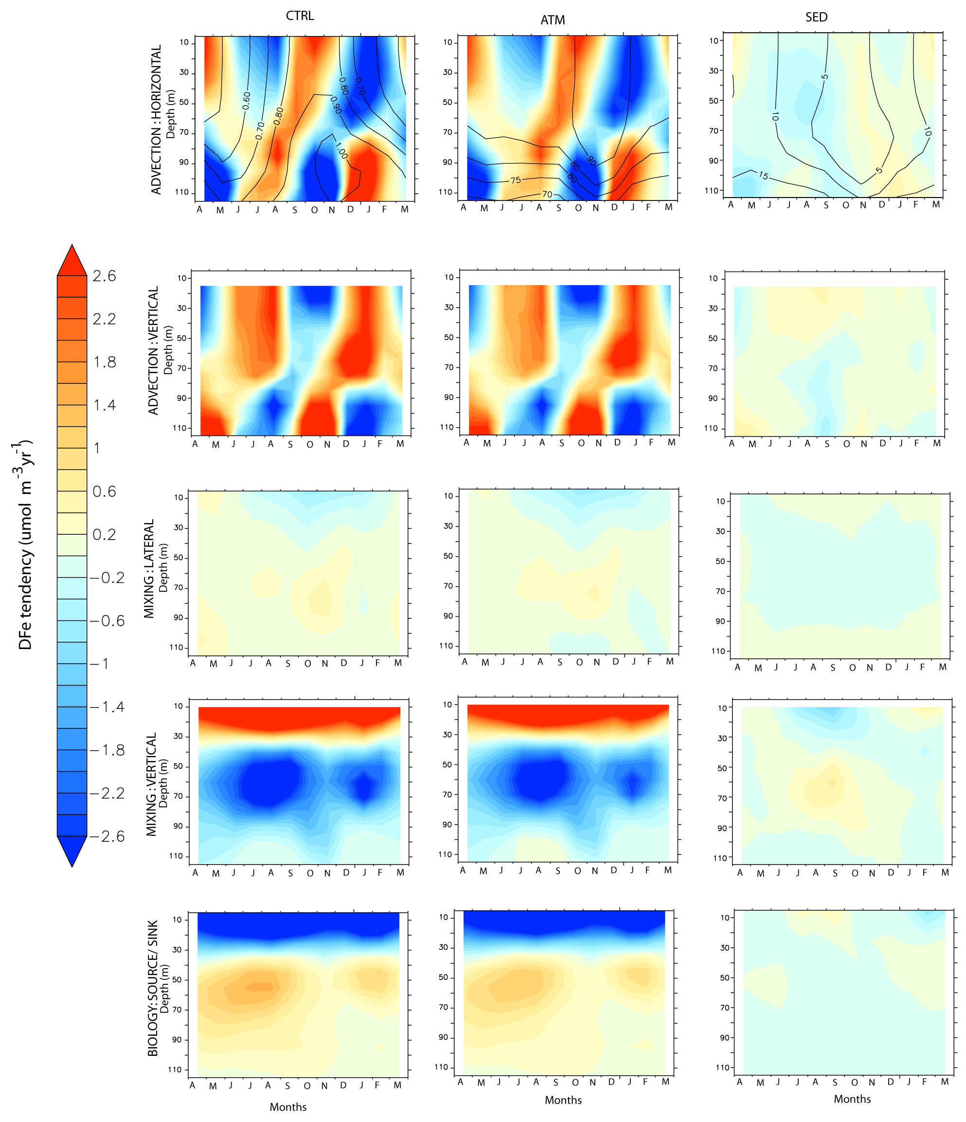
3.4.3 Central equatorial IO
With chlorophyll concentrations around 0.1 mg m−3 for most of the year, the central equatorial IO (2∘ S–2∘ N and 76–80∘ E) is the least productive of all the regions considered (Fig. 9d). Unlike its counterparts in the Pacific and the Atlantic oceans, the equatorial IO experiences only transient upwelling due to changes in wind direction associated with the migration of the intertropical convergence zone. This also leads to surface currents reversing their direction four times a year. Thus, the region experiences westward surface currents of weak magnitude during the southwest and northeast monsoon months and much stronger eastward current during the spring and fall intermonsoon months (Han et al., 1999). These narrow eastward surface currents during the intermonsoon months, known as the Wyrtki Jets, are in response to westerly winds (Wyrtki, 1973). The biogeochemical characteristics of the region have only been recently explored with the help of satellite and in situ data (e.g., Prasanna Kumar et al., 2012; Strutton et al., 2015). Deepening of the surface layer associated with the eastward transport of water during the intermonsoon months lowers productivity (Prasanna Kumar et al., 2012). Chlorophyll concentrations, although much lower compared to the rest of the IO, peak during October–December, possibly due to wind stirring or shear instability at the base of the eastward-moving Wyrtki Jet (Strutton et al., 2015). Additionally, in situ measurements in the central equatorial IO have revealed deep chlorophyll maxima, located at ∼ 60 m depth, that contribute to more than 30 % of the total chlorophyll biomass (Vidya et al., 2013). The peak ocean DFe concentration is encountered during August–November. Overall, the comparison between the CTRL, ATM, and SED cases show that atmospheric deposition, peaking during July (Fig. 9d), dominates the DFe contribution to the central equatorial IO, whereas the sedimentary DFe plays a distant secondary role (Fig. 12).
Horizontal advection is the most important process of DFe supply within the mixed layer during March–May and September–November (Fig. 12). During the intervening months, vertical advection plays the predominant role in DFe supply. Decomposing the horizontal advection further into DFe′ and U′ reveals that the meridional velocity convergence is the main contributor to the central equatorial IO DFe budget during March–May and September–November (Fig. S14 in the Supplement). This originates from the westerly wind directing equatorward Ekman flow in both the hemispheres, which leads to convergence and drives eastward-propagating downwelling Kelvin waves (McPhaden et al., 2015). Averaged over the upper 100 m, zonal velocity convergence, although of somewhat lower magnitude, opposes meridional velocity convergence throughout the year. When the Wyrtki Jet weakens, upwelling induced by easterly wind drives upward vertical supply of DFe, whereas there is downward vertical removal of DFe during the intervening periods. This alternation between upwelling and downwelling control on DFe has an upward phase propagation. An important feature of the central equatorial IO, in contrast to other equatorial regions, is the presence of the transient Equatorial Undercurrent between 60–200 m depth, the core of which is generally centered at the depth of the 20 ∘C isotherm (Chen et al., 2015). The Equatorial Undercurrent appears most strongly during winter–spring months and with much weaker magnitude during summer–fall months (Chen et al., 2015; Schott and McCreary, 2001). The CESM simulation reveals the signature of the upper part of the Equatorial Undercurrent in influencing the DFe budget. This is characterized by the zonal velocity underneath the mixed layer (∼ 80 m depth) showing strong eastward transport during January–April and a much weaker eastward transport during September–November. The horizontal convergence of DFe is prominent during the developing phase of the Equatorial Undercurrent (December–February and June–August), probably in association with the progressive eastward extension and strengthening of the Equatorial Undercurrent from the western IO. These periods of horizontal DFe convergence are interspersed with vertical DFe convergence. Superimposed on advection, vertical mixing plays an important role in bringing subsurface DFe to the surface levels in the upper 30 m, peaking during July–August.
Biological removal of DFe, almost entirely by small phytoplankton, is conspicuous in the upper 40 m and peaks during September. This is in line with sediment trap studies over the central equatorial IO, where peak biogenic fluxes are detected during the southwest and fall intermonsoon months and are dominated by coccolithophorids and foraminifera carbonate (Ramaswamy and Gaye, 2006). Furthermore, in situ water samples have shown that picoplankton, having sizes of less than 10 µm, constitute more than 90 % of the phytoplankton biomass in the central equatorial IO (Vidya et al., 2013). The period of peak biogenic flux is also characterized by a peak in DFe removal by scavenging and remineralization of particulate iron released from mortality and grazing at deeper layers (Fig. S16c in the Supplement). A secondary increase in the biological removal of DFe is noticed during January–March in association with a secondary peak in chlorophyll, although its impact is not evident in sediment trap biogenic-flux data (Vidya et al., 2013). This might arise from the remineralization of particulate iron being almost twice the magnitude of scavenging losses during this time of the year.
3.4.4 Central southern tropical IO
The central southern tropical IO (13–17∘ S and 72-76∘ E) is located in the transition zone between the DFe-poor region of the subtropical IO gyre and the DFe-enriched northern IO. Of all the regions considered, this receives the lowest atmospheric DFe (Fig. 9e), resulting in DFe limitation of phytoplankton growth, particularly during the boreal summer (Fig. 7). Steady southeasterly winds, prevailing throughout the year, transport dust from Australian sources into this region. The peak in dust deposition is during austral spring and summer in association with strong source activity (Kok et al., 2021; Yang et al., 2021). A secondary peak in dust deposition during austral winter is possibly associated with enhanced transport. The northern part of the central southern tropical IO lies on the Seychelles–Chagos thermocline ridge, which is characterized by doming up of the thermocline due to negative wind stress curl resulting in Ekman divergence (Vialard et al., 2009). The thermocline progressively deepens towards the sub-tropical southern IO gyre to the south as wind stress curl changes sign to positive. The westward-flowing South Equatorial Current brings low-salinity water and nutrients from the Indonesian region. Satellite-observed enhanced chlorophyll concentrations during the boreal (austral) summer (winter) months have been attributed to vertical diffusion (Końe et al., 2009; Lévy et al., 2007). Additionally, westward-propagating upwelling and/or downwelling Rossby waves arrive in this region following La Nina and/or El Nino events and play a key role in modulating sea surface height and the depth of thermocline (Masumoto and Meyers, 1998; Périgaud and Delecluse, 1992). This perturbs the depth of the nitracline, which has a significant impact on column productivity (Kawamiya and Oschlies, 2001).
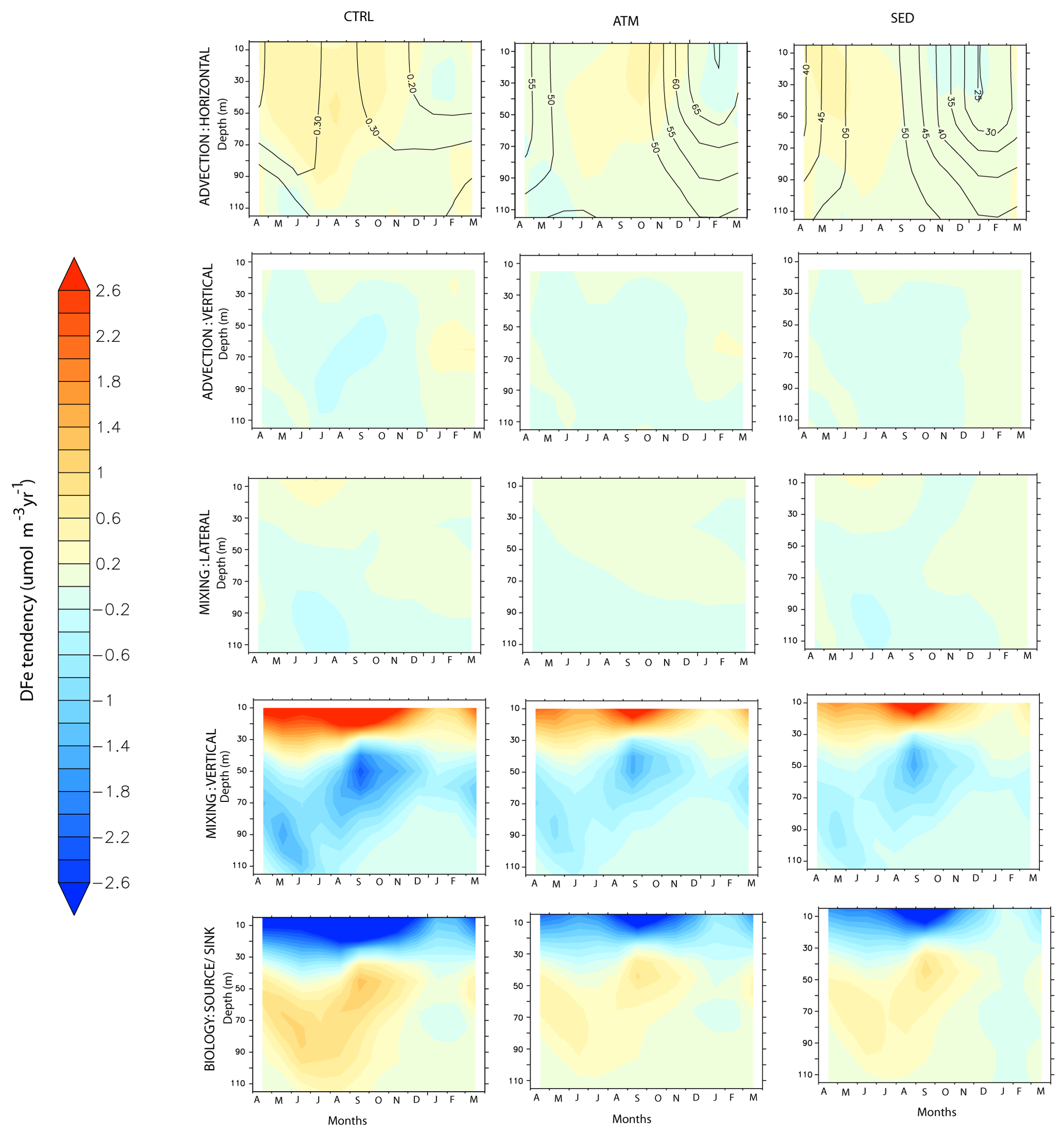
Both ATM and SED sources are important in this region for DFe supply, with the SED (ATM) source having a higher contribution during austral winter (summer) months (Fig. 13). Analysis of the CESM-simulated DFe budget reveals that vertical mixing in the upper 30 m is the most important process of DFe supply, which peaks during September. This is the time of the year when CESM records the lowest sea surface temperature resulting in mixed-layer deepening. Such winter mixing leads to the erosion of the vertical gradient in DFe observed during the rest of the year in the upper 120 m. Horizontal advection is the next most important supplier of DFe in this region. The westward-flowing South Equatorial Current is strongest during austral winter and during winter-to-summer transition months. This results in meridional velocity convergence and zonal velocity divergence, resulting in a quasi-balance between DFe supply and removal (Fig. S15 in the Supplement). Overall, horizontal advection leads to predominantly sedimentary DFe convergence during March–June and predominantly atmospheric DFe convergence during September–November.
The wind stress curl is mostly negative, that is upwelling favorable, throughout the year. Between April–October (austral winter), when winter convection-driven blooms are prominent, wind stress curl becomes weakly negative to slightly positive. Following this, during January–March, the wind stress curl becomes strongly negative, resulting in upward velocity, and favors vertical advection of both atmospheric and sedimentary DFe in equal magnitude. While vertical U′ is responsible for supplying DFe in the upper 50 m, vertical DFe′ is important at deeper depths (Fig. S15 in the Supplement).
The biological sink of DFe peaks during the month of maximum vertical mixing, that is, during September. During this time, the uptake of DFe is dominated by diatoms, which accounts for more than 80 % of the total DFe uptake. Small phytoplankton dominate the rest of the year. Scavenging removal of DFe and particulate iron remineralization peak 1 month later during October between 50–90 m depth (Fig. S16d in the Supplement). Overall, the central southern tropical IO is the only region where atmospheric deposition and sedimentary sources of iron are equally important in driving the DFe budget.
Using the ocean component of the Earth system model CESM version 2.1, this study elucidates the impacts of various sources of DFe on upper-ocean productivity, nutrient limitations, and DFe budgets over the northern IO. The iron cycle in CESM represents the complex interplay between several processes including DFe supply, removal by scavenging and biological uptake, particulate iron remineralization, and organic-ligand complexation. The major sources of DFe for this region are included in this model, namely atmospheric deposition, sediments, hydrothermal vents, and rivers. Although there are model biases in representing physical and biogeochemical variables, the overall patterns of the spatial and temporal variation of DFe are simulated reasonably well in CESM.
The study finds that atmospheric deposition is the most important source of DFe to the northern IO. Atmospheric deposition contributes well over 50 % of the total DFe concentration and more than 10 % (35 %) to the upper-100 m (surface-level) chlorophyll concentrations, especially over the AS, the equatorial IO, and the southern tropical IO. Sedimentary sources become important along continental shelves, where they can contribute to more than 20 % of the total DFe. The sedimentary source has the largest impact in fueling phytoplankton blooms over the southern tropical IO during June–September. In contrast, hydrothermal and river sources have negligible impacts on upper-ocean DFe pools in this region. Almost all regions that experience significant positive chlorophyll responses to atmospheric and sedimentary sources of DFe show a preponderance of diatoms over other phytoplankton groups. The increases in phytoplankton following external DFe addition are evoked in regions with low background DFe levels (< 0.3 nM) and high initial NO3:DFe, indicating the importance of high levels of macronutrients. Following the external DFe addition, a shift to nitrate limitation of phytoplankton is observed.
Analysis of the DFe budget across different biophysical regimes in the northern IO shows that this budget is generally dominated by atmospheric deposition, with sedimentary sources of DFe being a distant second contributor. The exception to this occurs over the southern tropical IO region, where both atmospheric and sedimentary sources become equally important. In all the regions considered, vertical mixing is the most important physical mechanism through which DFe is supplied, and furthermore, this mechanism is active almost throughout the year. In contrast, the importance of horizontal and vertical advection is highly seasonal. DFe uptake by small phytoplankton in the upper ocean is the most important route through which DFe removal takes place, except in the productive waters where diatoms also participate in the removal process. At subsurface levels, competition between the removal of DFe by scavenging and the remineralization of particulate iron determines the DFe pool available to the surface ocean via these aforementioned physical processes.
Of all DFe sources, atmospheric deposition is most likely to be vulnerable to future global warming, and changes to it will perhaps exert a strong influence on upper-ocean productivity and nutrient limitation. Additionally, 59 % of the continental shelves and bathyal seafloor over the northern IO experiences hypoxic conditions (Helly and Levin, 2004), and there are several lines of evidence pointing to reductions in oxygen content over this region during the last few decades due to enhanced upper-ocean stratification (Schmidtko et al., 2017). This will possibly impact the flux of iron from reduced sediments. The present study thus provides foundations to explore how different future scenarios of atmospheric deposition and the extent of reducing sediments can impact biogeochemistry over the northern IO.
Climatologies of ocean temperature, salinity, and nutrients are from the World Ocean Atlas 2018, available at https://www.ncei.noaa.gov/access/world-ocean-atlas-2018/ (last access: 15 June 2021). Monthly surface chlorophyll data from OC-CCI are obtainable from https://www.oceancolour.org/ (last access: 13 June 2022). The monthly climatology of ocean mixed-layer depth based on Holte et al. (2017) is downloadable from http://mixedlayer.ucsd.edu/ (last access: 1 September 2021). Surface ocean current data from OSCAR can be downloaded from https://podaac.jpl.nasa.gov/dataset/OSCAR_L4_OC_third-deg?ids =Keywords:Keywords:Projects&values=Oceans::Solid%20Earth:: OSCAR&provider=PODAAC (last access: 4 September 2021).
Dissolved iron data from the GEOTRACES Intermediate Data Product 2021 are available at https://www.geotraces.org/geotraces-intermediate-data-product-2021/ (last access: 15 March 2022). Additionally, dissolved-iron profile data are also obtainable from Tagliabue et al. (2012), available at https://www.bodc.ac.uk/geotraces/data/historical/ (last access: 1 July 2022). The code for CESM2.1 can be downloaded from https://www.cesm.ucar.edu/models/cesm2/release_download.html (last access: 1 December 2020).
The supplement related to this article is available online at: https://doi.org/10.5194/bg-20-2613-2023-supplement.
The author has declared that there are no competing interests.
Publisher's note: Copernicus Publications remains neutral with regard to jurisdictional claims in published maps and institutional affiliations.
Priyanka Banerjee acknowledges the computational facilities provided by the Supercomputer Education and Research Centre (SERC) at the Indian Institute of Science for carrying out the CESM simulations. Priyanka Banerjee is also grateful to Anh Pham, Nicola Wiseman, and an anonymous reviewer for the constructive comments, which have significantly improved this paper.
This research has been supported by the Department of Science and Technology, Ministry of Science and Technology, India (grant no. DST/INSPIRE/04/2018/002625).
This paper was edited by Peter Landschützer and reviewed by Nicola Wiseman, Anh Pham, and one anonymous referee.
Anand, S. S., Rengarajan, R., Sarma, V. V. S. S., Sudheer, A. K., Bhushan, R., and Singh, S. K.: Spatial variability of upper ocean POC export in the Bay of Bengal and the Indian Ocean determined using particle-reactive 234Th, J. Geophys. Res.-Oceans, 122, 3753–3770, https://doi.org/10.1002/2016JC012639, 2017.
Anand, S. S., Rengarajan, R., Shenoy, D., Gauns, M., and Naqvi, S. W. A.: POC export fluxes in the Arabian Sea and the Bay of Bengal: A simultaneous and study, Mar. Chem., 198, 70–87, https://doi.org/10.1016/j.marchem.2017.11.005, 2018.
Anderson, L. and Sarmiento, J.: Redfield ratios of remineralization determined by nutrient data analysis, Global Biogeochem. Cy., 8, 65–80, https://doi.org/10.1029/93GB03318, 1994.
Armstrong, R. A., Lee, C., Hedges, J. I., Honjo, S., and Wakeham, S.: A new, mechanistic model for organic carbon fluxes in the ocean: based on the quantitative association of POC with ballast minerals, Deep-Sea Res., 49, 219–236, 2002.
Banerjee, P. and Kumar, S. P.: Dust-induced episodic phytoplankton blooms in the Arabian Sea during winter monsoon, J. Geophys. Res.-Oceans, 119, 7123–7138, https://doi.org/10.1002/2014JC010304, 2014.
Banerjee, P., Satheesh, S. K., Moorthy, K. K., Nanjundiah, R. S., and Nair, V. S.: Long-range transport of mineral dust to the northeast Indian Ocean: Regional versus remote sources and the implications, J. Climate, 32, 1525–1549, https://doi.org/10.1175/JCLI-D-18-0403.1, 2019.
Barber, R. T., Marra, J., Bidigare, R. C., Codispoti, L. A., Halpern, D., Johnson, Z., Latasa, M., Goericke, R., and Smith, S. L.: Primary productivity and its regulation in the Arabian Sea during 1995, Deep-Sea Res. Pt. II, 48, 1127–1172, https://doi.org/10.1016/S0967-0645(00)00134-X, 2001.
Beal, L. M., Ffield, A., and Gordon, A. L.: Spreading of Red Sea overflow waters in the Indian Ocean, J. Geophys. Res., 105, 8549–8564, https://doi.org/10.1029/1999JC900306, 2000.
Bianchi, D., Dunne, J. P., Sarmiento, J. L., and Galbraith, E. D.: Data-based estimates of suboxia, denitrification, and N2O production in the ocean and their sensitivities to dissolved O2, Global Biogeochem. Cy., 26, GB2009, https://doi.org/10.1029/2011gb004209, 2012.
Blain, S., Quéguiner, B., Armand, L., Belviso, S., Bombled, B., Bopp, L., Bowie, A., Brunet, C., Brussaard, C., Carlotti, F., Christaki, U., Corbière, A., Durand, I., Ebersbach, F., Fuda, J.-L., Garcia, N., Gerringa, L., Griffiths, B., Guigue, C., Guillerm, C., Jacquet, S., Jeandel, C., Laan, P., Lefèvre, D., Lo Monaco, C., Malits, A., Mosseri, J., Obernosterer, I., Park, Y.-H., Picheral, M., Pondaven, P., Remenyi, T., Sandroni, V., Sarthou, G., Savoye, N., Scouarnec, L., Souhaut, M., Thuiller, D., Timmermans, K., Trull, T., Uitz, J., van Beek, P., Veldhuis, M., Vincent, D., Viollier, E., Vong, L., and Wagener, T.: Effect of natural iron fertilization on carbon sequestration in the Southern Ocean, Nature, 446, 1070–1074, https://doi.org/10.1038/nature05700, 2007.
Boss, E. and Behrenfeld, M.: In situ evaluation of the initiation of the North Atlantic phytoplankton bloom, Geophys. Res. Lett., 37, L18603, https://doi.org/10.1029/2010GL044174, 2010.
Boyd, P. W. and Ellwood, M. J.: The biogeochemical cycle of iron in the ocean, Nat. Geosci., 3, 675–682, https://doi.org/10.1038/ngeo964, 2010.
Buck, K. N., Lohan, M. C., Berger, C. J., and Bruland, K. W.: Dissolved iron speciation in two distinct river plumes and an estuary: Implications for riverine iron supply, Limnol. Oceanogr., 52, 843–855, https://doi.org/10.4319/lo.2007.52.2.0843, 2007.
Buesseler, K., Ball, L., Andrews, J., Benitez-Nelson, C., Belastock, R., Chai, F., and Chao, Y.: Upper ocean export of particulate organic carbon in the Arabian Sea derived from thorium-234, Deep-Sea Res. Pt. II, 45, 2461–2487, https://doi.org/10.1016/S0967-0645(98)80022-2, 1998.
Canfield, D. E.: The geochemistry of river particulates from the continental USA: Major elements, Geochim. Cosmochim. Ac., 61, 3349–3365, https://doi.org/10.1016/s0016-7037(97)00172-5, 1997.
Chen, G., Han, W., Li, Y., Wang, D., and McPhaden, M. J.: Seasonal-to-interannual time-scale dynamics of the equatorial undercurrent in the Indian Ocean, J. Phys. Oceanogr., 45, 1532–1553, https://doi.org/10.1175/JPO-D-14-0225.1, 2015.
Chinni, V. and Singh, S. K.: Dissolved iron cycling in the Arabian Sea and sub-tropical gyre region of the Indian Ocean, Geochim. Cosmochim. Ac., 317, 325–348, https://doi.org/10.1016/j.gca.2021.10.026, 2022.
Chinni, V., Singh, S. K., Bhushan, R., Rengarajan, R., and Sarma, V. V. S. S.: Spatial variability in dissolved iron concentrations in the marginal and open waters of the Indian Ocean, Mar. Chem., 208, 11–28, https://doi.org/10.1016/j.marchem.2018.11.007, 2019.
Conway, T. M. and John, S. G.: Quantification of dissolved iron sources to the North Atlantic Ocean, Nature, 511, 212–215, https://doi.org/10.1038/nature13482, 2014.
Dai, A., Qian, T., Trenberth, K. E., and Milliman, J. D.: Changes in continental freshwater discharge from 1948 to 2004, J. Climate, 22, 2773–2792, https://doi.org/10.1175/2008JCLI2592.1, 2009.
Danabasoglu, G., Bates, S. C., Briegleb, B. P., Jayne, S. R., Jochum, M., Large, W. G., Peacock, S., and Yeager, S. G.: The CCSM4 ocean component, J. Climate, 25, 1361–1389, https://doi.org/10.1175/JCLI-D-11-00091.1, 2012.
Danabasoglu, G., Lamarque, J.-F., Bacmeister, J., Bailey, D. A., DuVivier, A. K. , Edwards, J., Emmons, L. K., Fasullo, J., Garcia, R., Gettelman, A., Hannay, C., Holland, M. M., Large, W. G., Lauritzen, P. H., Lawrence, D. M., Lenaerts, J. T. M., Lindsay, K., Lipscomb, W. H., Mills, M. J., Neale, R., Oleson, K. W., Otto-Bliesner, B., Phillips, A. S., Sacks, W., Tilmes, S., van Kampenhout, L., Vertenstein, M., Bertini, A., Dennis, J., Deser, C., Fischer, C., Fox-Kemper, B., Kay, J. E., Kinnison, D., Kushner, P. J., Larson, V. E., Long, M. C., Mickelson, S., Moore, J. K., Nienhouse, E., Polvani, L., Rasch, P. J., and Strand, W. G.: The Community Earth System Model Version 2 (CESM2), J. Adv. Model. Earth Sy., 12, e2019MS001916, https://doi.org/10.1029/2019MS001916, 2020.
de Baar, H. J. W., Boyd, P. W., Coale, K. H., Landry, M. R., Tsuda, A., Assmy, P., Bakker, D. C. E., Bozec, Y., Barber, R. T., Brzezinski, M. A., Buesseler, K. O., Boye, M., Croot, P. L., Gervais, F., Gorbunov, M. Y., Harrison, P. J., Hiscock, W. T., Laan, P., Lancelot, C., Law, C. S., Levasseur, M., Marchetti, A., Millero, F. J., Nishioka, J., Nojiri, Y., van Oijen, T., Riebesell, U., Rijkenberg, M. J. A., Saito, H., Takeda, S., Timmermans, K. R., Veldhuis, M. J. W., Waite, A. M., and Wong, C.-S.: Synthesis of iron fertilization experiments: From the Iron Age in the Age of Enlightenment, J. Geophys. Res., 110, C09S16, https://doi.org/10.1029/2004JC002601, 2005.
de Baar, H., Gerringa, L., Laan, P., and Timmermans, K.: Efficiency of carbon removal per added iron in ocean iron fertilization, Mar. Ecol. Prog. Ser., 364, 269–282, https://doi.org/10.3354/meps07548, 2008.
Dohan, K. and Maximenko, N.: Monitoring ocean currents with satellite sensors, Oceanography, 23, 94–103, 2010.
Dutkiewicz, S., Ward, B. A., Monteiro, F., and Follows, M. J.: Interconnection between nitrogen fixers and iron in the Pacific Ocean: Theory and numerical model, Global Biogeochem. Cy., 26, GB1012, https://doi.org/10.1029/2011GB004039, 2012.
Elrod, V. A., Berelson, W. M., Coale, K. H., and Johnson, K. S.: The flux of iron from continental shelf sediments: A missing source for global budgets, Geophys. Res. Lett., 31, L12307, https://doi.org/10.1029/2004GL020216, 2004.
Gamo, T., Okamura, K., Hatanaka, H., Hasumoto, H., Komatsu, D., Chinen, M., Mori, M.,Tanaka, J., Hirota, A. and Tsunogai, U.: Hydrothermal plumes in the Gulf of Aden, as characterized by light transmission, Mn, Fe, CH4 and delta13C-CH4 anomalies, Deep-Sea Res. Pt. II, 121, 62–70, 2015.
Garcia, H. E., Locarnini, R. A., Boyer, T. P., Antonov, J. I., Baranova, O. K., Zweng, M. M., Reagan, J. R., and Johnson, D. R.: World Ocean Atlas 2013, Volume 3: Dissolved Oxygen, Apparent Oxygen Utilization, and Oxygen Saturation, edited by: Levitus, S. and Mishonov, A., NOAA Atlas NESDIS, 75, Washington, DC: NOAA, 27 pp., 2014a.
Garcia, H. E., Locarnini, R. A., Boyer, T. P., Antonov, J. I., Baranova, O. K., Zweng, M. M., Reagan, J. R., and Johnson, D. R.: World Ocean Atlas 2013, Volume 4: Dissolved Inorganic Nutrients (phosphate, nitrate, silicate), edited by: Levitus, S. and Mishonov, A., NOAA Atlas NESDIS, 76, Washington, DC: NOAA, 25 pp., 2014b.
Garcia H. E., Boyer, T. P., Baranova, O. K., Locarnini, R. A., Mishonov, A. V., Grodsky, A., Paver, C. R., Weathers, K. W., Smolyar, I. V., Reagan, J. R., Seidov, D., and Zweng, M. M.: World Ocean Atlas 2018: Product Documentation, edited by: Mishonov, A., NOAA/NESDIS, Silver Spring, MD, 2019.
Geider, R. J. and La Roche, J.: The role of iron in phytoplankton photosynthesis, and the potential for iron-limitation of primary productivity in the sea, Photosynth. Res., 39, 275–301, https://doi.org/10.1007/bf00014588, 1994.
Gent, P. R. and McWilliams, J. C.: Isopycnal mixing in ocean circulation models, J. Phys. Oceanogr., 20, 150–155, https://doi.org/10.1175/1520-0485(1990)020<0150:IMIOCM>2.0.CO;2, 1990.
GEOTRACES Intermediate Data Product Group: The GEOTRACES Intermediate Data Product 2021 (IDP2021), NERC EDS British Oceanographic Data Centre NOC, https://doi.org/10.5285/cf2d9ba9-d51d-3b7c-e053-8486abc0f5fd, 2021.
Grand, M. M., Measures, C. I., Hatta, M., Hiscock, W. T., Buck, C. S., and Landing, W. M.: Dust deposition in the eastern Indian Ocean: The ocean perspective from Antarctica to the Bay of Bengal, Global Biogeochem. Cy., 29, 357–374, https://doi.org/10.1002/2014gb004898, 2015.
Guieu, C., Al Azhar, M., Aumont, O., Mahowald, N., Lévy, M., Éthé, C., and Lachkar, Z.: Major impact of dust deposition on the productivity of the Arabian Sea, Geophys. Res. Lett., 46, 6736–6744, 2019.
Gustafsson, O., Kruså, M., Zencak, Z., Sheesley, R. J., Granat, L., Engström, E., Praveen, P. S., Rao, P. S., Leck, C., and Rodhe, H.: Brown clouds over South Asia: biomass or fossil fuel combustion?, Science, 323, 495–498, https://doi.org/10.1126/science.1164857, 2009.
Haake, B., Ittekkot, V., Rixen, T., Ramaswamy, V., Nair, R. R., and Curry, W. B.: Seasonality and interannual variability of particle fluxes to the deep Arabian Sea, Deep-Sea Res. Pt. I, 40, 1323–1344, 1993.
Han, W., McCreary, J. P., Anderson, D. L. T., and Mariano, A. J.: Dynamics of the eastern surface jets in the equatorial Indian Ocean, J. Phys. Oceanogr., 29, 2191–2209, https://doi.org/10.1175/1520-0485(1999)029<2191:DOTESJ>2.0.CO;2, 1999.
Harrison, C. S., Long, M. C., Lovenduski, N. S., and Moore, J. K.: Mesoscale Effects on Carbon Export: A Global Perspective, Global Biogeochem. Cy., 32, 680–703, https://doi.org/10.1002/2017GB005751, 2018.
Helly, J. J. and Levin, L. A.: Global distribution of naturally occurring marine hypoxia on continental margins, Deep-Sea Res. Pt. I, 51, 1159–1168, 2004.
Holte, J., Talley, L. D., Gilson, J., and Roemmich, D.: An Argo mixed layer climatology and database, Geophys. Res. Lett., 44, 5618–5626, https://doi.org/10.1002/2017GL073426, 2017.
Huffman, G. J., Adler, R. F., Arkin, P., Chang, A., Ferraro, R., Gruber, A., Janowiak, J., McNab, A., Rudolf, B., and Schneider, U.: The Global Precipitation Climatology Project (GPCP) Combined Precipitation Dataset, B. Am. Meteorol. Soc., 78, 5–20, https://doi.org/10.1175/1520-0477(1997)078<0005:TGPCPG>2.0.CO;2, 1997.
Ilyina, T., Six, K. D., Segschneider, J., Maier-Reimer, E., Li, H., and Núñez-Riboni, I.: Global ocean biogeochemistry model HAMOCC: Model architecture and performance as component of the MPI-Earth system model in different CMIP5 experimental realizations, J. Adv. Model. Earth Sy., 5, 287–315, https://doi.org/10.1029/2012MS000178, 2013.
Jickells, T. D., An, Z. S., Andersen, K. K., Baker, A. R., Bergametti, G., Brooks, N., Cao, J. J., Boyd, P. W., Duce, R. A., Hunter, K. A., Kawahata, H., Kubilay, N., laRoche, J., Liss, P. S., Mahowald, N., Prospero, J. M., Ridgwell, A. J., Tegen, I., and Torres, R.: Global Iron Connections between Desert Dust, Ocean Biogeochemistry, and Climate, Science, 308, 67–71, 2005.
Jin, Q., Wei, J., Pu, B., Yang, Z. L., and Parajuli, S. P.: High summertime aerosol loadings over the Arabian Sea and their transport pathways, J. Geophys. Res.-Atmos., 123, 10568–10590, https://doi.org/10.1029/2018jd028588, 2018.
Johnson, K. S., Chavez, F. P., and Friederich, G. E.: Continental-shelf sediment as a primary source of iron for coastal phytoplankton, Nature, 398, 697–700, https://doi.org/10.1038/19511, 1999.
Kalnay, E., Kanamitsu, M., Kistler, R., Collins, W., Deaven, D., Gandin, L., Iredell, M., Saha, S., White, G., Woollen, J., Zhu, Y., Leetmaa, A., Reynolds, R., Chelliah, M., Ebisuzaki, W., Higgins, W., Janowiak, J., Mo, K. C., Ropelewski, C., Wang, J., Jenne, R., and Joseph, D.: The NCEP/NCAR 40-Year Reanalysis Project, B. Am. Meteorol. Soc., 77, 437–471, https://doi.org/10.1175/1520-0477(1996)077<0437:TNYRP>2.0.CO;2, 1996.
Kawamiya, M. and Oschlies, A.: Formation of a basin-scale surface chlorophyll pattern by Rossby waves, Geophys. Res. Lett., 28, 4139–4142, 2001.
Kohfeld, K. E. and Harrison, S. P.: DIRTMAP: the geological record of dust, Earth-Sci. Rev., 54, 81–114, https://doi.org/10.1016/S0012-8252(01)00042-3, 2001.
Kok, J. F., Adebiyi, A. A., Albani, S., Balkanski, Y., Checa-Garcia, R., Chin, M., Colarco, P. R., Hamilton, D. S., Huang, Y., Ito, A., Klose, M., Li, L., Mahowald, N. M., Miller, R. L., Obiso, V., Pérez García-Pando, C., Rocha-Lima, A., and Wan, J. S.: Contribution of the world's main dust source regions to the global cycle of desert dust, Atmos. Chem. Phys., 21, 8169–8193, https://doi.org/10.5194/acp-21-8169-2021, 2021.
Końe, V., Aumont, O., Lévy, M., and Resplandy, L.: Physical and Biogeochemical Controls of the Phytoplankton Seasonal Cycle in the Indian Ocean: A Modeling Study, Geoph. Monog. Series, 185, 147–166, https://doi.org/10.1029/2008GM000700, 2009.
Kumar, A., Suresh, K., and Rahaman, W.: Geochemical Characterization of Modern Aeolian Dust over the Northeastern Arabian Sea: Implication for Dust Transport in the Arabian Sea, Sci. Total Environ., 729, 138576, https://doi.org/10.1016/j.scitotenv.2020.138576, 2020.
Kuttippurath, J., Sunanda, N., Martin, M. V., and Chakraborty, K.: Tropical storms trigger phytoplankton blooms in the deserts of north Indian Ocean, NPJ Climate and Atmospheric Science, 4, 11, https://doi.org/10.1038/s41612-021-00166-x, 2021.
Large, W. G. and Yeager, S. G.: The global climatology of an interannually varying air-sea flux data set, Clim. Dynam., 33, 341–364, https://doi.org/10.1007/s00382-008-0441-3, 2009.
Large, W. G., McWilliams, J. C., and Doney, S. C.: Oceanic vertical mixing: A review and a model with a nonlocal boundary layer parameterization, Rev. Geophys., 32, 363–403, 1994.
Léon, J. F. and Legrand, M.: Mineral dust sources in the surroundings of the North Indian Ocean, Geophys. Res. Lett., 30, 1309, https://doi.org/10.1029/2002GL016690, 2003.
Letelier, R. M., Karl, D. M., Abbott, M. R., and Bidigare, R. R.: Light driven seasonal patterns of chlorophyll and nitrate in the lower euphotic zone of the North Pacific Subtropical Gyre, Limnol. Oceanogr., 49, 508–519, https://doi.org/10.4319/lo.2004.49.2.0508, 2004.
Levitus, S., Boyer, T., Concright, M., Johnson, D., O'Brien, T., Antonov, J., Stephens, C., and Garfield, R.: Introduction, Vol. I, World Ocean Database 1998, NOAA Atlas NESDIS 18, US Government Printing Office, Washington, DC, 346 pp, 1998.
Lévy, M., Shankar, D., André, J., Shenoi, S., Durand, F., and de Boyer Montégut, C.: Basin-wide seasonal evolution of the Indian Ocean's phytoplankton blooms, J. Geophys. Res.-Oceans, 112, C12014, https://doi.org/10.1029/2007JC004090, 2007.
Liu, J. P., Xue, Z., Ross, K.,Wang, H. J., Yang, Z. S., and Gao, S.: Fate of sediments delivered to the sea by Asian large rivers: Long-distance transport and formation of remote alongshore clinothems, Sedimentary Record, 7, 4–9, https://doi.org/10.2110/sedred.2009.4.4, 2009.
Liu, X., Ma, P.-L., Wang, H., Tilmes, S., Singh, B., Easter, R. C., Ghan, S. J., and Rasch, P. J.: Description and evaluation of a new four-mode version of the Modal Aerosol Module (MAM4) within version 5.3 of the Community Atmosphere Model, Geosci. Model Dev., 9, 505–522, https://doi.org/10.5194/gmd-9-505-2016, 2016.
Long, M. C., Moore, J. K., Lindsay, K., Levy, M. N., Doney, S. C., Luo, J. Y., Krumhardt, K. M., Letscher, R. T., Grover, M., and Sylvester, Z. T.: Simulations with the Marine Biogeochemistry Library (MARBL), J. Adv. Model. Earth Sy., accepted, https://doi.org/10.1029/2021MS002647, 2021.
Madhu, N., Jyothibabu, R., Maheswaran, P., Gerson, V. J., Gopalakrishnan, T., and Nair, K.: Lack of seasonality in phytoplankton standing stock (chlorophyll a) and production in the western Bay of Bengal, Cont. Shelf Res., 26, 1868–1883, 2006.
Madhupratap, M., Prasanna Kumar, S., Bhattathiri, P. M. A., DileepKumar, M., Raghukumar, S., Nair, K. K. C., and Ramaiah, N.: Mechanism of the biological response to winter cooling in the northeastern Arabian Sea, Nature, 384, 549–552, 1996.
Madhupratap, M., Gauns, M., Ramaiah, N., Kumar, S. P., Muraleedharan, P., de Sousa, S., Sardessai, S., and Muraleedharan, U.: Biogeochemistry of the Bay of Bengal: physical, chemical and primary productivity characteristics of the central and western Bay of Bengal during summer monsoon 2001, Deep-Sea Res. Pt. II, 50, 881–896, https://doi.org/10.1016/S0967-0645(02)00611-2, 2003.
Mahowald, N. M., Engelstaedter, S., Luo, C., Sealy, A., Artaxo, P., Benitez-Nelson, C., Bonnet, S., Chen, Y., Chuang, P. Y., Cohen, D. D., Dulac, F., Herut, B., Johansen, A. M., Kubilay, N., Losno, R., Maenhaut, W., Paytan, A., Prospero, J. M., Shank, L. M., and Siefert, R. L.: Atmospheric iron deposition: global distribution, variability, and human perturbations, Annu. Rev. Mar. Sci., 1, 245–278, https://doi.org/10.1146/annurev.marine.010908.163727, 2009.
Masumoto, Y. and Meyers, G.: Forced Rossby waves in the southern tropical Indian Ocean, J. Geophys. Res.-Oceans, 103, 27589–27602, https://doi.org/10.1029/98JC02546, 1998.
Mayorga, E., Seitzinger, S. P., Harrison, J. A., Dumont, E., Beusen, A. H. W., Bouwman, A. F., Fekete, B. M., Kroeze, C. and van Drecht, G.: Global Nutrient Export from WaterSheds 2 (NEWS 2): Model development and implementation, Environ. Modell. Softw., 25, 837–853, https://doi.org/10.1016/j.envsoft.2010.01.007, 2010.
McLennan, S. M.: Relationships between the trace element composition of sedimentary rocks and upper continental crust, Geochem. Geophy. Geosy., 2, 1021, https://doi.org/10.1029/2000gc000109, 2001.
McPhaden, M. J., Wang, Y., and Ravichandran, M.: Volume transports of the Wyrtki jets and their relationship to the Indian Ocean dipole, J. Geophys. Res.-Oceans, 120, 5302–5317, 2015.
Measures, C. I. and Vink, S.: Seasonal variations in the distribution of Fe and Al in the surface waters of the Arabian Sea, Deep-Sea Res. Pt. II, 46, 1597–1622, 1999.
Mills, M. M., Ridame, C., Davey, M., La Roche, J., and Geider, R. J.: Iron and phosphorus co-limit nitrogen fixation in the eastern tropical North Atlantic, Nature, 429, 292, https://doi.org/10.1038/nature02550, 2004.
Moffett, J. W., Goepfert, T. J., and Naqvi, S. W. A.: Reduced iron associated with secondary nitrite maxima in the Arabian Sea, Deep-Sea Res. Pt. I, 54, 1341–1349, https://doi.org/10.1016/j.dsr.2007.04.004, 2007.
Moffett, J. W., Vedamati, J., Goepfert, T. J., Pratihary, A., Gauns, M., and Naqvi, S. W. A.: Biogeochemistry of iron in the Arabian Sea, Limnol. Oceanogr., 60, 1671–1688, https://doi.org/10.1002/lno.10132, 2015.
Moore, C. M., Mills, M. M., Achterberg, E. P., Geider, R. J., La Roche, J., Lucas, M. I., McDonagh, E. I., Pan, X., Poulton, A. J., and Rijkenberg, M. J.: Large-scale distribution of Atlantic nitrogen fixation controlled by iron availability, Nat. Geosci., 2, 867–871, 2009.
Moore, C. M., Mills, M. M., Arrigo, K. R., Berman-Frank, I., Bopp, L., Boyd, P. W., Galbraith, E. D., Geider, R. J., Guieu, C., Jaccard, S. L., Jickells, T. D., Roche, J. L., Lenton, T. M., Mahowald, N. M., Marañón, E., Marinov, I., Moore, J. K., Nakatsuka, T., Oschlies, A., Saito, M. A., Thingstad, T. F., Tsuda, A., and Ulloa, O.: Processes and patterns of oceanic nutrient limitation, Nat. Geosci., 6, 701–710, https://doi.org/10.1038/NGEO1765, 2013.
Moore, J. K. and Braucher, O.: Sedimentary and mineral dust sources of dissolved iron to the world ocean, Biogeosciences, 5, 631–656, https://doi.org/10.5194/bg-5-631-2008, 2008.
Moore, J. K., Doney, S. C., and Lindsay, K.: Upper ocean ecosystem dynamics and iron cycling in a global three-dimensional model, Global Biogeochem. Cy., 18, GB4028, https://doi.org/10.1029/2004GB002220, 2004.
Moore, J. K., Lindsay, K., Doney, S. C., Long, M. C., and Misumi, K.: Marine Ecosystem Dynamics and Biogeochemical Cycling in the Community Earth System Model CESM1(BGC): Comparison of the 1990s with the 2090s under the RCP4.5 and RCP8.5 Scenarios, J. Climate, 26, 9291–9312, https://doi.org/10.1175/jcli-d-12-00566.1, 2013.
Moorthy, K. K. and Babu, S. S.: Aerosol black carbon over Bay of Bengal observed from an island location, Port Blair: Temporal features and long-range transport, J. Geophys. Res., 111, D17205, https://doi.org/10.1029/2005JD006855, 2006.
Morrison, J. M., Codispoti, L. A., Gaurin, S., Jones, B., Manghanani, V., and Zheng, Z.: Seasonal variations of hydrographic and nutrient fields during the US JGOFS Arabian Sea Process Study, Deep-Sea Res. Pt. II, 45, 2053–2101, 1998.
Morrison, J. M., Codispoti, L. A., Smith, S. L., Wishner, K., Flagg, C., Gardner, W. D., Gaurin, S., Naqvi, S., Manghnani, V., Prosperie, L., and Gundersen, J. S.: The oxygen minimum zone in the Arabian Sea during 1995, Deep-Sea Res. Pt. II, 46, 1903–1931, 1999.
Naqvi, S. W. A., Moffett, J. W., Gauns, M. U., Narvekar, P. V., Pratihary, A. K., Naik, H., Shenoy, D. M., Jayakumar, D. A., Goepfert, T. J., Patra, P. K., Al-Azri, A., and Ahmed, S. I.: The Arabian Sea as a high-nutrient, low-chlorophyll region during the late Southwest Monsoon, Biogeosciences, 7, 2091–2100, https://doi.org/10.5194/bg-7-2091-2010, 2010.
Nishioka, J., Obata, H., and Tsumune, D.: Evidence of an extensive spread of hydrothermal dissolved iron in the Indian Ocean, Earth Planet. Sc. Lett., 361, 26–33, https://doi.org/10.1016/j.epsl.2012.11.040, 2013.
Olsen, A., Key, R. M., van Heuven, S., Lauvset, S. K., Velo, A., Lin, X., Schirnick, C., Kozyr, A., Tanhua, T., Hoppema, M., Jutterström, S., Steinfeldt, R., Jeansson, E., Ishii, M., Pérez, F. F., and Suzuki, T.: The Global Ocean Data Analysis Project version 2 (GLODAPv2) – an internally consistent data product for the world ocean, Earth Syst. Sci. Data, 8, 297–323, https://doi.org/10.5194/essd-8-297-2016, 2016.
Périgaud, C. and Delecluse, P.: Annual sea level variations in the southern tropical Indian Ocean from Geosat and shallow water simulations, J. Geophys. Res., 97, 20169–20178, https://doi.org/10.1029/92JC01961, 1992.
Pham, A. L. D. and Ito, T.: Anthropogenic iron deposition alters the ecosystem and carbon balance of the Indian Ocean over a centennial timescale, J. Geophys. Res.-Oceans, 126, e2020JC016475, https://doi.org/10.1029/2020JC016475, 2021.
Pollard, R. T., Salter, I., Sanders, R. J., Lucas, M. I., Moore, C. M., Mills, R. A., Statham, P. J., Allen, J. T., Baker, A. R., Bakker, D. C. E., Charette, M. A., Fielding, S., Fones, G. R., French, M., Hickman, A. E., Holland, R. J., Hughes, J. A., Jickells, T. D., Lampitt, R. S., Morris, P. J., Nedelec, F. H., Nielsdottir, M., Planquette, H., Popova, E. E., Poulton, A. J., Read, J. F., Seeyave, S., Smith, T., Stinchcombe, M., Taylor, S., Thomalla, S., Venables, H. J., Williamson, R., and Zubkov, M. V.: Southern Ocean deep-water carbon export enhanced by natural iron fertilization, Nature, 457, 577–580, https://doi.org/10.1038/nature07716, 2009.
Prasanna Kumar, S., Madhupratap, M., Dileep Kumar, M., Muraleedharan, P. M., de Souza, S. N., Gauns, M., and Sarma, V. V. S. S.: High biological productivity in the central Arabian Sea during summer monsoon driven by Ekman pumping and lateral advection, Curr. Sci.-India, 81, 1633–1638, 2001.
Prasanna Kumar, S., Nuncio, M., Narvekar, J., Kumar, A., Sardesai, S., de Souza, S. N., Gauns, M., Ramaiah, N., and Madhupratap, M.: Are eddies nature's trigger to enhance biological productivity in the Bay of Bengal?, Geophys. Res. Lett., 31, L07309, https://doi.org/10.1029/2003GL019274, 2004.
Prasanna Kumar, S., Divya David, T., Byju, P., Narvekar, J., Yoneyama, K., Nakatani, N., Ishida, A., Horii, T., Masumoto, Y., and Mizuno, K.: Bio-physical coupling and ocean dynamics in the central equatorial Indian Ocean during 2006 Indian Ocean Dipole, Geophys. Res. Lett., 39, L14601, https://doi.org/10.1029/2012GL052609, 2012.
Ramaswamy, V. and Gaye, B.: Regional variations in the fluxes of foraminifera carbonate, coccolithophorid carbonate and biogenic opal in the northern Indian Ocean, Deep-Sea Res. Pt. I, 53, 271–293, https://doi.org/10.1016/j.dsr.2005.11.003, 2006.
Ramaswamy, V., Gaye, B., Shirodkar, P. V., Rao, P. S., Chivas, A. R., Wheeler, D., and Thwin, S.: Distribution and sources of organic carbon, nitrogen and their isotopic signatures in sediments from the Ayeyarwady (Irrawaddy) continental shelf, northern Andaman Sea, Mar. Chem., 111, 137–150. https://doi.org/10.1016/j.marchem.2008.04.006, 2008.
Raven, J. A.: The iron and molybdenum use efficiencies of plant growth with different energy, carbon and nitrogen sources, New Phytol., 109, 279–287, https://doi.org/10.1111/j.1469-8137.1988.tb04196.x, 1988.
Redi, M. H.: Oceanic isopycnal mixing by coordinate rotation, J. Phys. Oceanogr., 12, 1154–1158, https://doi.org/10.1175/1520-0485(1982)012<1154:OIMBCR>2.0.CO;2, 1982.
Resplandy, L., Lévy, M., Madec, G., Pous, S., Aumont, O., and Kumar, D.: Contribution of mesoscale processes to nutrient budgets in the Arabian Sea, J. Geophys. Res., 116, C11007, https://doi.org/10.1029/2011JC007006, 2011.
Rixen, T., Gaye, B., and Emeis, K.-C.: The monsoon, carbon fluxes, and the organic carbon pump in the northern Indian Ocean, Prog. Oceanogr., 175, 24–39, https://doi.org/10.1016/j.pocean.2019.03.001, 2019.
Robinson, R. A. J., Bird, M. I., Oo, N. W., Hoey, T. B., Aye, M. M., Higgitt, D. L., Lud, X. X., Swe, A., Tun, T., and Win, S. L.: The Irrawaddy river sediment flux to the Indian Ocean: the original nineteenth-century data revisited, J. Geol., 115, 629–640, https://doi.org/10.1086/521607, 2007.
Sander, S. and Koschinsky, A.: Metal flux from hydrothermal vents increased by organic complexation, Nat. Geosci., 4, 145–150, https://doi.org/10.1038/ngeo1088, 2011.
Sathyendranath, S., Brewin, R. J., Brockmann, C., Brotas, V., Calton, B., Chuprin, A., Cipollini, P., Couto, A. B., Dingle, J., Doerffer, R., Donlon, C., Dowell, M., Farman, A., Grant, M., Groom, S., Horseman, A., Jackson, T., Krasemann, H., Lavender, S., Martinez-Vicente, V., Mazeran, C., Mélin, F., Moore, T. S., Müller, D., Regner, P., Roy, S., Steele, C. J., Steinmetz, F., Swinton, J., Taberner, M., Thompson, A., Valente, A., Zühlke, M., Brando, V. E., Feng, H., Feldman, G., Franz, B. A., Frouin, R., Gould, R. W., Hooker, S. B., Kahru, M., Kratzer, S., Mitchell, B. G., Muller-Karger, F. E., Sosik, H. M., Voss, K. J., Werdell, J., and Platt, T.: An Ocean-Colour Time Series for Use in Climate Studies: The Experience of the Ocean-Colour Climate Change Initiative (OC-CCI), Sensors, 19, 4285, https://doi.org/10.3390/s19194285, 2019.
Schlosser, C., Klar, J. K., Wake, B. D., Snow, J. T., Honey, D. J., Woodward, E. M. S., Lohan, M. C., Achterberg, E. P., and Moore, C. M.: Seasonal ITCZ migration dynamically controls the location of the (sub)tropical Atlantic biogeochemical divide, P. Natl. Acad. Sci. USA, 111, 1438–1442, 2014.
Schmidtko, S., Stramma, L., and Visbeck, M.: Decline in global oceanic oxygen content during the past five decades, Nature, 542, 335–339, https://doi.org/10.1038/nature21399, 2017.
Schott, F. and McCreary, J. P.: The monsoon circulation of the Indian Ocean, Prog. Oceanogr., 51, 1–123, https://doi.org/10.1016/S0079-6611(01)00083-0, 2001.
Sedwick, P. N. and DiTullio, G. R.: Regulation of algal blooms in Antarctic shelf waters by the release of iron from melting sea ice, Geophys. Res. Lett., 24, 2515–2518, https://doi.org/10.1029/97GL02596, 1997.
Singh, N. D., Chinni, V., and Singh, S. K.: Dissolved aluminium cycling in the northern, equatorial and subtropical gyre region of the Indian Ocean, Geochim. Cosmochim. Ac., 268, 160–185, https://doi.org/10.1016/j.gca.2019.09.028, 2020.
Sholkovitz, E. R., Sedwick, P. N., Church, T. M., Baker, A. R., and Powell, C. F.: Fractional solubility of aerosol iron: Synthesis of a global-scale data set, Geochim. Cosmochim. Ac., 89, 173–189, https://doi.org/10.1016/j.gca.2012.04.022, 2012.
Smith, R., Jones, P., Briegleb, B., Bryan, F., Danabasoglu, G., Dennis, J., Dukowicz, J., Eden, C., Fox-Kemper, B., Gent, P., Hecht, M., Jayne, S., Jochum, M., Large, W., Lindsay, K., Maltrud, M., Norton, N., Peacock, S., Vertenstein, M., and Yeager, S.: The Parallel Ocean Program (POP) reference manual, Ocean component of the Community Climate System Model (CCSM), LANL Tech. Report, LAUR-10-01853, National Center for Atmospheric Research, Boulder, CO, USA, 141 pp., 2010.
Smith, S. L.: Understanding the Arabian Sea: Reflections on the 1994–1996 Arabian Sea Expedition, Deep-Sea Res. Pt. II, 48, 1385–1402, 2001.
Srinivas, B. and Sarin, M. M.: Atmospheric dry-deposition of mineral dust and anthropogenic trace metals to the Bay of Bengal, J. Mar. Syst., 126, 56–68, https://doi.org/10.1016/j.jmarsys.2012.11.004, 2013.
Srinivas, B., Sarin, M. M., and Kumar, A.: Impact of anthropogenic sources on aerosol iron solubility over the Bay of Bengal and the Arabian Sea, Biogeochemistry, 110, 257–268, https://doi.org/10.1007/s10533-011-9680-1, 2012.
Strutton, P. G., Coles, V. J., Hood, R. R., Matear, R. J., McPhaden, M. J., and Phillips, H. E.: Biogeochemical variability in the central equatorial Indian Ocean during the monsoon transition, Biogeosciences, 12, 2367–2382, https://doi.org/10.5194/bg-12-2367-2015, 2015.
Sunda, W. G. and Huntsman, S. A.: Iron uptake and growth limitation in oceanic and coastal phytoplankton, Mar. Chem., 50, 189–206, https://doi.org/10.1016/0304-4203(95)00035-P, 1995.
Tagliabue, A., Bopp, L., Dutay, J.-C., Bowie, A. R., Chever, F., Jean-Baptiste, P., Bucciarelli, E., Lannuzel, D., Remenyi, T., Sarthou, G., Aumont, O., Gehlen, M., and Jeandel, C.: Hydrothermal contribution to the oceanic dissolved iron inventory, Nat. Geosci., 3, 252–256, https://doi.org/10.1038/ngeo818, 2010.
Tagliabue, A., Mtshali, T., Aumont, O., Bowie, A. R., Klunder, M. B., Roychoudhury, A. N., and Swart, S.: A global compilation of dissolved iron measurements: focus on distributions and processes in the Southern Ocean, Biogeosciences, 9, 2333–2349, https://doi.org/10.5194/bg-9-2333-2012, 2012.
Tagliabue, A., Aumont, O., and Bopp, L.: The impact of different external sources of iron on the global carbon cycle, Geophys. Res. Lett., 41, 920–926, https://doi.org/10.1002/2013GL059059, 2014.
Tagliabue, A., Aumont, O., De'Ath, R., Dunne, J. P., Dutkiewicz, S., Galbraith, E., Misumi, K., Moore, J. K., Ridgwell, A., Sherman, E., Stock, C., Vichi, M., Völker, C., and Yool, A.: How well do global ocean biogeochemistry models simulate dissolved iron distributions?, Global Biogeochem. Cy., 30, 149–174, https://doi.org/10.1002/2015GB005289, 2016.
Takeda, S., Kamarani, A., and Kawanobe, K.: Effects of nitrogen and iron entichments on phytoplankton communities, Mar. Chem., 50, 229–241, https://doi.org/10.1016/0304-4203(95)00038-S,1995.
Thushara, V., Vinayachandran, P. N. M., Matthews, A. J., Webber, B. G. M., and Queste, B. Y.: Vertical distribution of chlorophyll in dynamically distinct regions of the southern Bay of Bengal, Biogeosciences, 16, 1447–1468, https://doi.org/10.5194/bg-16-1447-2019, 2019.
Twining, B. S., Rauschenberg, S., Morton, P. L., and Vogt, S.: Metal contents of phytoplankton and labile particulate material in the North Atlantic Ocean, Progr. Oceanogr., 137, 261–283, https://doi.org/10.1016/j.pocean.2015.07.001, 2015.
Twining, B. S., Rauschenberg, S., Baer, S. E., Lomas, M. W., Martiny, A. C., and Antipova, O. M.: A nutrient limitation mosaic in the eastern tropical Indian Ocean, Deep-Sea Res. Pt. II, 166, 125–140, https://doi.org/10.1016/j.dsr2.2019.05.001, 2019.
Twining, B. S., Antipova, O., Chappell, P. D., Cohen, N. R., Jacquot, J. E., Mann, E. L., Marchetti, A., Ohnemus, D. C., Rauschenberg, S., and Tagliabue, A.: Taxonomic and nutrient controls on phytoplankton iron quotas in the ocean, Limnology and Oceanography Letters, 6, 96–106, https://doi.org/10.1002/lol2.10179, 2021.
Unger, D., Ittekkot, V., Schäfer, P., Tiemann, J., and Reschke, S.: Seasonality and interannual variability of particle fluxes to the deep Bay of Bengal: influence of riverine input and oceanographic processes, Deep-Sea Res. Pt. II, 50, 897–923, 2003.
Vialard, J., Duvel, J. P., McPhaden, M. J., Bouruet-Aubertot, P., Ward, B., Key, E., Bourras, D., Weller, R., Minnett, P., Weill, A., Cassou, C., Eymard, L., Fristedt, T., Basdevant, C., Dandonneau, Y., Duteil, O., Izumo, T., de Boyer Montégut, C., Masson, S., and Kennan, S.: Cirene: Air–Sea Interactions in the Seychelles – Chagos Thermocline Ridge Region, B. Am. Meteorol. Soc., 90, 45–62, https://doi.org/10.1175/2008BAMS2499.1, 2009.
Vidya, P. J. and Prasanna Kumar, S.: Role of mesoscale eddies on the variability of biogenic flux in the northern and central Bay of Bengal, J. Geophys. Res.-Oceans, 118, 5760–5771, https://doi.org/10.1002/jgrc.20423, 2013.
Vidya, P. J., Prasanna Kumar, S., Gauns, M., Verenkar, A., Unger, D., and Ramaswamy, V.: Influence of physical and biological processes on the seasonal cycle of biogenic flux in the equatorial Indian Ocean, Biogeosciences, 10, 7493–7507, https://doi.org/10.5194/bg-10-7493-2013, 2013.
Vinayachandran, P. N., Chauhan, P., Mohan, M., and Nayak, S.: Biological response of the sea around Sri Lanka to summer monsoon, Geophys. Res. Lett., 31, L0I302, https://doi.org/10.1029/2003GL018533, 2004.
Vinayachandran, P. N., Shankar, D., Vernekar, S., Sandeep, K. K., Amol, P., Neema, C. P., and Chatterjee, A.: A summer monsoon pump to keep the Bay of Bengal salty, Geophys. Res. Lett., 40, 1777–1782, https://doi.org/10.1002/grl.50274, 2013.
Vu, H. and Sohrin, Y.: Diverse stoichiometry of dissolved trace metals in the Indian Ocean, Sci. Rep.-UK, 3, p. 1745, https://doi.org/10.1038/srep01745, 2013.
Wang, S., Bailey, D., Lindsay, K., Moore, J. K., and Holland, M.: Impact of sea ice on the marine iron cycle and phytoplankton productivity, Biogeosciences, 11, 4713–4731, https://doi.org/10.5194/bg-11-4713-2014, 2014.
Webber, B. G. M., Matthews, A. J., Vinayachandran, P. N., Neema, C. P., Sanchez-Franks, A., Vijith, V., Amol, P., and Baranowski, D. B.: The dynamics of the Southwest Monsoon current in 2016 from high-resolution in situ observations and models, J. Phys. Oceanogr., 48, 2259–2282, https://doi.org/10.1175/JPO-D-17-0215.1, 2018.
Wiggert, J. D., and Murtugudde, R. G.: The sensitivity of the Southwest Monsoon phytoplankton bloom to variations in aeolian iron deposition over the Arabian Sea, J. Geophys. Res., 112, C05005, https://doi.org/10.1029/2006JC003514, 2007.
Wyrtki, K.: An equatorial jet in the Indian Ocean, Science, 181, 262–264, https://doi.org/10.1126/science.181.4096.262, 1973.
Xie, P. and Arkin, P. A.: Global precipitation: A 17-year monthly analysis based on gauge observations, satellite estimates, and numerical model outputs, B. Am. Meteorol. Soc., 78, 2539–2558, https://doi.org/10.1175/1520-0477(1997)078<2539:GPAYMA>2.0.CO;2, 1997.
Yang, X., Zhao, C., Yang, Y., and Fan, H.: Long-term multi-source data analysis about the characteristics of aerosol optical properties and types over Australia, Atmos. Chem. Phys., 21, 3803–3825, https://doi.org/10.5194/acp-21-3803-2021, 2021.
Yoon, J.-E., Yoo, K.-C., Macdonald, A. M., Yoon, H.-I., Park, K.-T., Yang, E. J., Kim, H.-C., Lee, J. I., Lee, M. K., Jung, J., Park, J., Lee, J., Kim, S., Kim, S.-S., Kim, K., and Kim, I.-N.: Reviews and syntheses: Ocean iron fertilization experiments – past, present, and future looking to a future Korean Iron Fertilization Experiment in the Southern Ocean (KIFES) project, Biogeosciences, 15, 5847–5889, https://doi.org/10.5194/bg-15-5847-2018, 2018.
Zhang, Y., Rossow, W. B., Lacis, A. A., Oinas, V., and Mishchenko, M. I.: Calculation of radiative fluxes from the surface to top of atmosphere based on ISCCP and other global data sets: Refinements of the radiative transfer model and the input data, J. Geophys. Res., 109, D19105, https://doi.org/10.1029/2003JD004457, 2004.