A differentiable, physics-informed ecosystem modeling and learning framework for large-scale inverse problems: demonstration with photosynthesis simulations

Photosynthesis plays an important role in carbon, nitrogen, and water cycles. Ecosystem models for photosynthesis are characterized by many parameters that are obtained from limited in situ measurements and applied to the same plant types. Previous site-by-site calibration approaches could not leverage big data and faced issues like overfitting or parameter non-uniqueness. Here we developed an end-to-end programmatically differentiable (meaning gradients of outputs to variables used in the model can be obtained efficiently and accurately) version of the photosynthesis process representation within the Functionally Assembled Terrestrial Ecosystem Simulator (FATES) model. As a genre of physics-informed machine learning (ML), differentiable models couple physics-based formulations to neural networks (NNs) that learn parameterizations (and potentially processes) from observations, here photosynthesis rates. We first demonstrated that the framework was able to correctly recover multiple assumed parameter values concurrently using synthetic training data. Then, using a real-world dataset consisting of many different plant functional types (PFTs), we learned parameters that performed substantially better and greatly reduced biases compared to literature values. Further, the framework allowed us to gain insights at a large scale. Our results showed that the carboxylation rate at 25 ^∘C (V_c,max25) was more impactful than a factor representing water limitation, although tuning both was helpful in addressing biases with the default values. This framework could potentially enable substantial improvement in our capability to learn parameters and reduce biases for ecosystem modeling at large scales.

1 Introduction

Plant photosynthesis is critically important for regulating the global carbon and nutrient cycles, and thus the future climate. Understanding future climate trajectories requires understanding photosynthetic responses to changes in environmental factors including atmospheric CO₂ concentrations, radiation, temperature, humidity, and nutrient and water availability (Kirschbaum, 2004). Photosynthesis is influenced by many factors such as higher CO₂ levels, reduced productivity of vegetation (i.e., nutrient concentration; Thompson et al., 2017), intensified droughts (Urban et al., 2017; Xu et al., 2019), and rising temperatures (Dusenge et al., 2019) under a changing climate. To comprehensively evaluate the impacts of these changing processes and vegetation feedback to the atmosphere, we need accurate representations of photosynthesis in our models.

For global assessments of the carbon cycle, vegetation models were developed to simulate terrestrial ecosystem processes and the distributions of vegetation, both vertically in the soil–plant system and horizontally across the landscape. Substantial efforts over the last few decades have improved the representation of vegetation and its responses and feedback to climate change (Fisher et al., 2018). A typical framework structure for vegetation models is to keep track of changes in carbon and optionally nutrient states, driven by climatic variables and modulated by soil properties, with feedback to the climate, e.g., CO₂ releases, radiation, and vegetation composition and structure. A core component of the vegetation module is photosynthesis (Quillet et al., 2010).

Present ecosystem models for photosynthesis are based primarily on mechanistic descriptions of plant photosynthesis pathways, but this theoretically sound modeling paradigm faces many challenges, with parametric uncertainty being a major one. Photosynthesis models may describe limitations of carboxylation rates, light availability, and plant-specific factors like enzyme efficiencies for C₃ and C₄ plants differently (Farquhar et al., 1980; Farquhar and Caemmerer, 1982; Meyer, 1983; Von Caemmerer, 2003, 2013; Yin and Struik, 2009). They contain many parameters that quantify these efficiencies and limitations. In the past, these parameters have been estimated from different approaches: (1) obtained from a limited set of in situ sites and scaled based on climate and environmental factors (Verheijen et al., 2013), (2) calibrated on observational data site by site or for a few sites for a specific plant functional type (PFT; Mäkelä et al., 2019; Wang et al., 2014), or (3) optimized based on environmental conditions (Ali et al., 2016). However, these estimated values may not be optimal at the global scale. Site-by-site calibrations using genetic or similar algorithms are highly expensive and are limited in their spatial coverage and generalizability to different PFTs and species. Furthermore, such calibration faces the issue of nonuniqueness (which some call equifinality; Beven and Freer, 2001), where different parameter sets produce the same outcome. As a result, calibration can easily lead to poorly generalizable parameter values. This problem exists for many domains with diverse parameters, including ecosystem modeling (Tang and Zhuang, 2008). It has been similarly found in hydrologic modeling and has troubled scientists there for decades (Beven, 2006). More recently, it has been possible for some parameters to be fitted directly from large datasets with directly measured parameter values (Luo et al., 2021), which is highly valuable but is limited to those parameters with extensive observations, e.g., soil water retention and hydraulic properties. An efficient way to permit large-scale inverse modeling is needed.

There has been substantial progress in utilizing modern machine learning (ML) for geosciences. Purely data-driven deep learning models (LeCun et al., 2015; Reichstein et al., 2019; Shen, 2018; Shen et al., 2018) directly learn from data so they tend to be fairly accurate, and many have outperformed traditional models for a large number of applications across domains such as hydrology (Feng et al., 2020, 2021; Rahmani et al., 2020, 2021; Liu et al., 2023; Wunsch et al., 2021; Fang and Shen, 2020), agriculture (ElSaadani et al., 2021; Hossain et al., 2019; Liu et al., 2022; Saleem et al., 2019), energy balance (Zhu et al., 2021), cryosphere (Leong and Horgan, 2020; Zhang et al., 2019), water quality (Hrnjica et al., 2021; Zhi et al., 2021; Saha et al., 2023; Zhi et al., 2023), and ecosystem modeling (Zhang et al., 2020, 2021). In particular, the loss function is defined on all data points and sites, enforcing stronger constraints and leading to the data synergy effect, where the model gains better performance as the amount of training data increases (Fang et al., 2022). Unfortunately, deep learning models also lack interpretability and process clarity, and can only output trained variables with extensive observations. This need for data is often not satisfied for ecological processes.

To aid geoscientific models in general, Tsai et al. (2021) presented an efficient framework known as differentiable parameter learning (dPL), in an effort to leverage recent progress in ML to mitigate the issues with parameter inversion discussed above. This framework turns parameter estimation into a large-scale ML problem. It is mainly composed of a parameter estimation module based on a neural network (NN), combined with a process-based model (PBM) or its surrogate. The whole framework must be “programmatically differentiable” (Baydin et al., 2018; Innes et al., 2019), which refers to a programming paradigm that can efficiently and accurately obtain the gradients of the outputs with respect to any of the variables used in the model (Shen et al., 2023). Once we have programmatic differentiability, dPL can efficiently learn unknown functions from big data to serve as either a parameterization or process representation. Tsai et al. (2021) found that this framework scales well with more data, produces spatially and temporally well-generalized parameter sets, extends well to uncalibrated variables, and saves orders of magnitude in computational time. Feng et al. (2022a) further showed that a differentiable process-based hydrologic model with dPL could approach the performance of a purely data-driven ML model, and potentially outperform ML in data-sparse regions (Feng et al., 2022b). These successes can be conveniently migrated to the ecosystem modeling domain.

Here, we applied the dPL framework to the leaf-scale photosynthesis module of the Functionally Assembled Terrestrial Ecosystem Simulator (FATES) model. FATES is an ecosystem model that describes coexistence and competition in PFTs (Koven et al., 2020). FATES can be used as an ecosystem module in the Community Land Model (CLM; Oleson et al., 2013; Lawrence et al., 2019) to represent ecosystem demography (Fisher et al., 2015). The photosynthesis module is based on the Farquhar photosynthesis model. To apply the dPL framework in our study, we first reimplemented the photosynthesis module from FATES so that it became programmatically differentiable. Second, we connected this model to NNs for parameter estimation. With this tool, we aimed to answer the following questions.

1. Are parameters like V_c,max25 and soil water limitation factor simultaneously identifiable?

2. What is the achievable model performance, in terms of predicting photosynthesis rates in space and time, by tuning the parameters for the classical photosynthesis module without changing the model structure?

3. Are parameters learned from a large global dataset similar to the values used in current models?

In the following, we first describe the photosynthesis model with different parameter estimation experiments and target datasets. We then discuss the parameters chosen to be estimated and their significance. Afterward, we present the results from synthetic experiments and experiments based on real datasets from sites around the globe. Finally, we compare the learned parameters to values from the literature and provide some suggestions for future work.

2 Methods and datasets

2.1 General overview

Our general framework trains connected NNs to provide parameters (and later process representations) to PBMs, in this case the photosynthesis module of the FATES ecosystem model, on all the training data points simultaneously (Fig. 1a). The NNs map from some raw inputs to some tuneable physical parameters (θ; later extensible to processes) required for the PBM. The predicted physical parameters are then fed into the differentiable PBM along with other required forcing variables (F) and untuned constant attributes (θ_c) to compute the simulated target variable (y_sim), which is compared with observations to compute a loss function. The forward run starts from the NN inputs and ends at the loss function (following the blue arrows in Fig. 1a); the model's goal is to minimize the output of the loss function. We then backpropagate the errors (shown by black arrows in Fig. 1a) through the PBM equations back to the NNs so we can train them using gradient descent. To support gradient-based training, the entire framework must be differentiable (Shen et al., 2023), which ensures that neither the NN nor the PBM is a black box – they both allow explicit inspection and modification of the internal structures. Thus, the photosynthesis module of FATES had to be reimplemented on a differentiable platform.

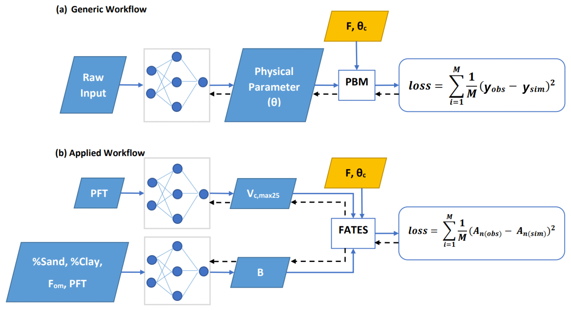
Figure 1 Diagram showing the dPL framework, which is a hybrid of NNs and the photosynthesis module in the FATES ecosystem model written on a differentiable platform. (a) The generic workflow: some raw information is mapped into physical parameters via an NN. These parameters are sent into a PBM, which then outputs the simulations, y_sim, that are compared with the observations, y_obs. Direct supervision for the physical parameters themselves is not required – we do not need ground truth values for these parameters. The loss function is “global” in that it involves all training data points, rather than being computed site-by-site as done in traditional calibration. (b) The workflow for the computational example described in this work. We estimate either V_c,max25 or the parameter B, or both of them at the same time, using NNs. The parameters are then fed into the differentiable photosynthesis module in FATES, which then outputs the net photosynthesis rate, A_n(sim), that is compared with A_n(obs). When not estimated from the data, default values from the literature were used. Blue arrows show the running of the NNs with the PBM in a forward (“prediction”) mode, while black arrows indicate backpropagation from the loss function back through the differentiable model equations to the NNs to update their weights, which is only done during initial NN training.

In this case, the PBM is the photosynthesis module in FATES, which can be written as a nonlinear system of equations, and its solution is implicit. The system can be written as

$$\begin{array}{}\text{(1)}& f\left(x;\mathit{\theta },{\mathit{\theta }}_{\mathrm{c}},F\right)=\mathrm{0};y=h\left(x,\mathit{\theta },{\mathit{\theta }}_{\mathrm{c}},F\right),\end{array}$$

where f represents the physical system constraint, h is an observation operator, x represents the unknowns of the equations (in this case the intercellular leaf CO₂ partial pressure, Pa), y is an observable variable (in this case net photosynthetic rate, µmol m⁻² s⁻¹) that is dependent on x via h, F represents some meteorological forcing variables such as radiation and air temperature, θ represents a list of tuneable physical parameters, and θ_c represents untuned constant attributes. Given a set of θ with known θ_c and F, we need to solve for x from f and send the solution into h to further compute y: $y=h\left(f^{-\mathrm{1}}\left(\mathit{\theta },{\mathit{\theta }}_{\mathrm{c}},F\right),\mathit{\theta },{\mathit{\theta }}_{\mathrm{c}},F\right)$.

This whole workflow can be lumped into one model:

$$\begin{array}{}\text{(2)}& y={\mathit{\delta }}_{\mathrm{psn}}\left(\mathit{\theta },{\mathit{\theta }}_{\mathrm{c}},F\right)\end{array}$$

where δ_psn represents the overall photosynthesis model. Some of the tuneable parameters are typically formulated as being PFT dependent (e.g., the maximum carboxylation rate at 25 ^∘C, V_c,max25), where each PFT includes groups of plant species that share similar physical and phenological characteristics leading to similar interactions with the environment. Other tuneable parameters are related to soil water availability (e.g., soil water stress parameters). We posit that there exists a parameterization scheme, θ=g^W(R), which is a mapping relationship of some underlying attributes R (e.g., soil attributes and plant traits) with the physical parameters represented by NN g with W learnable weights. Thus, we can learn W so that the simulated variable y matches the observations y^*:

$$\begin{array}{}\text{(3)}& W={\mathrm{argmin}}_W\left(L\left({\mathit{\delta }}_{\mathrm{psn}}\left(g^W\left(R\right),{\mathit{\theta }}_{\mathrm{c}},F\right),y^{\ast }\right)\right),\end{array}$$

where L is the loss function. For the purpose of solving the inverse problem and training the NN g^W in an “online” mode using gradient descent (the only practically employed algorithm for NN training), we reimplemented the photosynthesis module in FATES onto two differentiable platforms: Julia and PyTorch (discussed in more detail below).

In order to test the learning capability of our framework and the identifiability of the parameters, we first ran synthetic experiments to verify if the model would be able to correctly retrieve assumed values for the physical parameters. Second, using a dataset with thousands of photosynthesis rate measurements, we trained the differentiable model to obtain estimated parameters at the global scale, and compared them to the literature.

2.2 The Farquhar photosynthesis model

The FATES photosynthesis module is based on the classical Farquhar model for C₃ plants (Farquhar et al., 1980), which calculates the photosynthetic rate based on carbon fluxes under different limitations. For C₄ plants, it uses the Collatz model (Collatz et al., 1992). Both models assume that the gross photosynthetic rate is affected by the maximum rate of carboxylation and is limited by the concentration of RuBP carboxylase (Rubisco; A_c), light and electron transport (A_j), and the concentration of PEP carboxylase enzyme in C₄ plants (A_p). The final gross photosynthetic rate “A” is calculated using the empirical curvature parameters (θ_cj and θ_ip), while the net photosynthetic rate A_n is the same as the gross rate (A) after the plant respiration rate (R_d) is subtracted. The system can be described succinctly as the following, with Eqs. (4) and (5) playing the roles of f and h in Eq. (1), respectively; the whole set of associated equations is detailed in Fig. 2 and Appendix A.

$$\begin{array}{}\text{(4)}& {\displaystyle }{C}_{\mathrm{i}}=C_{\mathrm{a}}-A_{\mathrm{n}}{P}_{\mathrm{atm}}{\displaystyle \frac{(\mathrm{1.4}{g}_{\mathrm{s}}+\mathrm{1.6}{g}_{\mathrm{b}})}{(g_{\mathrm{s}}\times g_{\mathrm{b}})}},\text{(5)}& {\displaystyle }{A}_{\mathrm{n}}=A\left(C_{\mathrm{i}}\right)-R_d.\end{array}$$

Equation (4) is a single-variable nonlinear equation, with the intercellular leaf CO₂ pressure (C_i) as the unknown term to be solved (serving as the x term in Eq. 1). C_i is influenced by the CO₂ partial pressure near the leaf surface (C_a), the net photosynthetic rate (A_n), the atmospheric pressure (P_atm), the leaf stomatal conductance (g_s), and the leaf boundary layer conductance (g_b). Upon solving for C_i, we can further calculate A_n, which is the y term in Eq. (1). In the original implementations of FATES and CLM, the system of nonlinear equations was solved iteratively using fixed-point iteration (Oleson et al., 2013).

In order to train the physical equations and NNs together using gradient descent, the above equations were implemented on differentiable platforms to support backpropagation. We developed two alternative implementations: using PyTorch in Python (Paszke et al., 2019) and using Julia (Bezanson et al., 2012). The PyTorch version solves the coupled nonlinear equations using our parallel implementation of Newton iteration with automatic differentiation, while the Julia version uses adjoint-based methods implemented via a symbolic computer algebra system and is compatible with a wide variety of nonlinear solvers (Gowda et al., 2022). In contrast to the previous fixed-point iteration used by the original FATES model, our PyTorch Newton iteration solver can run on a graphical processing unit (GPU) in parallel for many sites. Newton's iteration method features second-order convergence compared to the slower convergence of fixed-point iteration, while GPU parallelism represents orders-of-magnitude savings in computational time compared to the original algorithm in FATES. The photosynthesis problem studied here has only one unknown (C_i) even though there are many other supporting equations, but we have successfully tested other larger nonlinear systems. Altogether, we can train this model with the coupled NNs for hundreds of data points in under 10 min (typically in 600 iterations) and could also train the model on 10 000 data points. For future work where time steps are involved, the adjoint method will likely be employed to reduce GPU memory use during nonlinear iterative solving. For the Julia implementation, the symbolic toolbox ModelingToolKit.jl (Gowda et al., 2022; Ma et al., 2022) was employed to automatically generate the solution scheme as Julia code, and along with solvers from NonlinearSolve.jl, solve the system of equations in the forward problem. Presently, we have implemented the Julia version in serial mode only. Results presented in this paper were produced using the PyTorch version, although the computational results were the same with the Julia version. Hence, we think both versions have value for future effort.

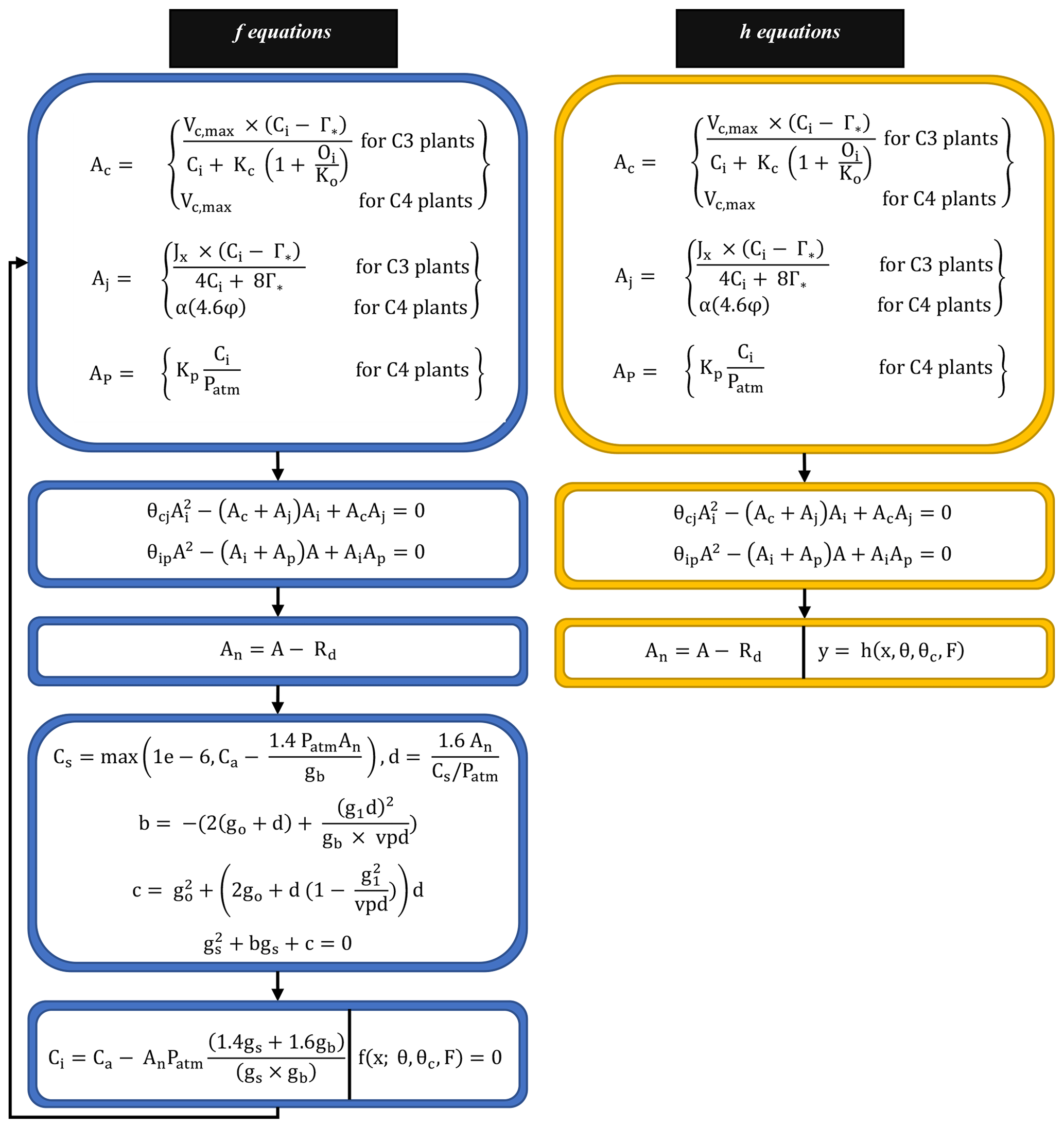
Figure 2 Model equations corresponding to f and h in Eq. (1). Blue boxes indicate equations corresponding to f. Yellow boxes indicate equations corresponding to h. First, we obtain a solution for C_i (intercellular leaf CO₂ pressure) by solving the nonlinear system (f equations) as illustrated in the last (bottom) blue box. Then, we run the h equations forward to compute A_n (net photosynthesis rate) using A_c, A_j, and A_p as discussed in Sect. 2.2. Details about different variables and parameters included in the f and h equations are provided in Appendix A.

2.3 The parameterization pipeline and model changes

We used multilayer perceptron (MLP) NNs as the parameterization module g in Eq. (3). The purpose of the MLPs is to estimate parameters θ, which are then fed into the photosynthesis module to obtain the net photosynthetic rate (A_n; Appendix A). The MLPs were trained based on minimization of the loss function – in brief, the goal is to minimize the difference between the solved and observed values of A_n. As described in Eq. (2), the whole workflow is hereafter referred to as the δ_psn model (“delta-photosynthesis model”; the Greek letter δ is selected because the model is programmatically differentiable and δ is often associated with gradients). There may be multiple MLPs used to estimate different parameters in θ, each with different inputs of either continuous or categorical data, and they can all be trained together. Figure 1a shows the general framework for parameter estimation experiments and panel (b) shows the framework of this particular work.

We chose to estimate one or both of two specific parameters in our experiments. The first one is the plant maximum carboxylation rate at 25 ^∘C (V_c,max25), which is normally formulated as a PFT-dependent parameter. Although V_c,max25 is hypothesized to be PFT dependent, recent studies have shown that the parameter can vary in space and time and by different species in the PFT as well (Ali et al., 2015; Chen et al., 2022; Qian et al., 2019). Estimating V_c,max25 is not a trivial matter due to its high variability and sensitivity to different factors such as drought, leading some studies to suggest a substitute. For example, Croft et al. (2017) suggested using leaf chlorophyll content as a direct proxy for V_c,max25. Nevertheless, considering this is an initial study applying dPL, we followed the convention and parameterized it based on PFT:

$$\begin{array}{}\text{(6)}& V_{\mathrm{c},\max \mathrm{25}}={\mathrm{NN}}_V\left(\mathrm{PFT}\right),\end{array}$$

where PFT is the plant functional type category (in one-hot encoding format, which translates each category to a binary vector) and the NN used for parameterization of V_c,max25 is referred to as NN_V hereafter.

The second parameterization is for parameter B defined by Clapp and Hornberger (1978), which influences the soil water stress function (β_t, where the subscript t indicates transpiration). β_t, called “btran” in the CLM code, reflects the impacts of soil wetness on stomatal conductance and ranges from zero (extreme dry conditions causing stomata closure) to one (wet conditions with stomata fully open). In the following, we describe B and β_t computations as in CLM4.5 (Oleson et al., 2013). B is purely a function of soil properties and is defined for each soil layer as B_i, where i refers to the soil layer (see Appendix B). B_i equations will later be replaced by our NN-based parameterization scheme as explained in Sect. 2.3.1 because they were originally empirical and may not be optimal at the global scale. B comes into play when calculating the soil water potential ψ_i using a power-law formulation:

$$\begin{array}{}\text{(7)}& {\mathit{\psi }}_i={\mathit{\psi }}_{\mathrm{sat},i}\times S_i^{-B_i}\ge {\mathit{\psi }}_{\mathrm{c}},\end{array}$$

where ψ_sat,i is the saturated soil matric potential and S_i is the soil wetness, both defined for a specific soil layer (see Appendix B for detailed calculations). The plant wilting factor (w_i) is then calculated using ψ_i and other PFT-dependent parameters (defined in CLM4.5) such as the soil matric potentials for closed stomata ψ_c and open stomata ψ_o, which represent the soil water potentials when stomata are fully closed and fully open, respectively, as defined in Eq. (8). The factor w_i is also dependent on other factors like the temperature of the soil layer (T_i) relative to the freezing temperature (T_f), the volumetric liquid water content (θ_liq), the volumetric ice content (θ_ice), and the volumetric water content at saturation (θ_sat). In our calculations, θ_ice was ignored since both the leaf and the air temperatures in our dataset were above freezing (0 ^∘C or 273.15 K) by at least 5 ^∘C.

$$\begin{array}{}\text{(8)}& w_i=\left\{\begin{array}{l}\frac{{\mathit{\psi }}_{\mathrm{c}}-{\mathit{\psi }}_i}{{\mathit{\psi }}_{\mathrm{c}}-{\mathit{\psi }}_{\mathrm{o}}}\left[\frac{{\mathit{\theta }}_{\mathrm{sat},i}-{\mathit{\theta }}_{\mathrm{ice},i}}{{\mathit{\theta }}_{\mathrm{sat},i}}\right]\le \mathrm{1};\\ T_i>T_{\mathrm{f}}-\mathrm{2}\text{and}{\mathit{\theta }}_{\mathrm{liq},i}>\mathrm{0}\\ \\ \mathrm{0};\\ T_i\le T_{\mathrm{f}}-\mathrm{2}\text{or}{\mathit{\theta }}_{\mathrm{liq},i}\le \mathrm{0}\end{array}\right\}.\end{array}$$

Finally, β_t can be calculated by aggregating the plant wilting factor (w_i) and plant root distribution (r_i) across different soil layers based on the PFT as

$$\begin{array}{}\text{(9)}& {\mathit{\beta }}_{\mathrm{t}}=\sum _i{w}_i{r}_i.\end{array}$$

2.3.1 Model changes

In the original water limitation function in CLM4.5, the stomata response to soil water potential is based on a linear function between the water potential for stomata openness and closedness (see Eq. 8). In light of the possibility that plants could respond differently to soil water potential depending on plant hydraulic traits (Christoffersen et al., 2016), in this study, we modified the soil water limitation for PFTs so that they could have different shapes. Specifically, we defined PFT-dependent soil water stress, ψ_i(PFT) ranging from ψ_c and ψ_o, depending on the soil water content, which is calculated as follows:

$$\begin{array}{}\text{(10)}& {\mathit{\psi }}_i\left(\mathrm{PFT}\right)={\mathit{\psi }}_{\mathrm{o}}\times S_i^{-B_i(\mathrm{soil},\mathrm{PFT})}\ge {\mathit{\psi }}_{\mathrm{c}}.\end{array}$$

B_i is a PFT- and soil-texture-dependent shape parameter (between 0 and 1) estimated as

$$\begin{array}{}\text{(11)}& B_i={\mathrm{NN}}_{B_i}(\mathit{\%}{\mathrm{sand}}_i,\mathit{\%}{\mathrm{clay}}_i,F_{\mathrm{om},i},\mathrm{PFT}),\end{array}$$

where %sand_i, %clay_i, and F_om,i respectively represent the percentage of sand, the percentage of clay, and the fraction of organic matter in soil layer i. The PFT-dependent soil water stress, ψ_i(PFT), is then fed into the plant wilting Eq. (8) as follows:

$$\begin{array}{}\text{(12)}& \begin{array}{rl}{w}_i& ={\displaystyle \frac{{\mathit{\psi }}_{\mathrm{c}}-{\mathit{\psi }}_i\left(\mathrm{PFT}\right)}{{\mathit{\psi }}_{\mathrm{c}}-{\mathit{\psi }}_{\mathrm{o}}}}\\ & ={\displaystyle \frac{{\mathit{\psi }}_{\mathrm{c}}-max\mathit{\psi }\left({\mathit{\psi }}_{\mathrm{c}},{\mathit{\psi }}_{\mathrm{o}}\times S_i^{-B_i(\mathrm{soil},\mathrm{PFT})}\right)}{{\mathit{\psi }}_{\mathrm{c}}-{\mathit{\psi }}_{\mathrm{o}}}}\le \mathrm{1}\end{array}.\end{array}$$

The new shape parameter B_i in Eq. (11) has a different range (between 0 and 1) from the original one defined by Clapp and Hornberger (1978) in Eq. (7), and it varies spatially for different static attributes and for different PFTs as well. The default equations in CLM4.5 for computations of B_i (Appendix B) show that the parameter B_i depends on two attributes, %clay_i and F_om,i, which is why they were used in NN${}_{B_i}$. To account for the dependence of ψ_sat,i on %sand_i (Appendix B) and its replacement by ψ_o (see Eqs. 7 and 10), %sand_i was also added to NN${}_{B_i}$. We also added PFT to NN${}_{B_i}$ inputs because vegetation may interact with the soil moisture constraint and we want to allow relevant factors to be included, rather than restricting the list of inputs to what was previously used in the literature. Since in NN${}_{B_i}$ we use quantitative inputs (%sand_i, %clay${}_i,F_{\mathrm{om},i}$) along with categorical inputs (PFT), we used the embedding layer in PyTorch, which translates each category to a vector of quantitative variables. This categorical data can then easily be combined with other quantitative inputs we provide to our NN.

Using the original Eq. (7) for computing ψ_i resulted in a plant wilting factor, w_i, equal to one for more than 90 % of the data points across different soil layers. Changing Eq. (7) to the form shown in Eq. (10) helped to express more variability in w_i and eventually in the computed soil water stress function (β_t).

2.4 Input and observation datasets

2.4.1 Forcing and photosynthesis rates

For meteorological forcings, we used the ERA5 Reanalysis dataset (Muñoz Sabater, 2019), which provides hourly estimates of soil moisture at different soil depths. Soil moisture contributes to the computation of β_t (see Appendix B), where the soil wetness S depends on both the soil moisture and the saturated soil moisture.

For observations of photosynthesis, we used data from the leaf gas exchange database (Knauer et al., 2018; Lin et al., 2015), which is a global database of stomatal conductance measurements and leaf-level photosynthetic rates. It incorporates data from several sites around the world in Australia, Europe, USA, and Asia (Fig. 3). We refer to this dataset as Lin15 throughout the rest of this work, with 43 sites chosen whose dates and times of measurements were available. Lin15 covered nine different PFT categories: rainfed crop “Crop R”, Broadleaf evergreen tree tropical “BET Tropical”, Broadleaf evergreen tree temperate “BET Temperate”, C₃ grass, C₄ grass, Needleleaf evergreen tree boreal “NET Boreal”, Needleleaf evergreen tree temperate “NET Temperate”, Broadleaf deciduous tree temperate “BDT Temperate”, and Broadleaf deciduous shrub temperate “BDS Temperate”. Measurements were taken on the sub-hourly scale but not necessarily at a continuous daily interval. That is why for almost all the sites, data were available on some random days (not necessarily continuous) for one or a few years.

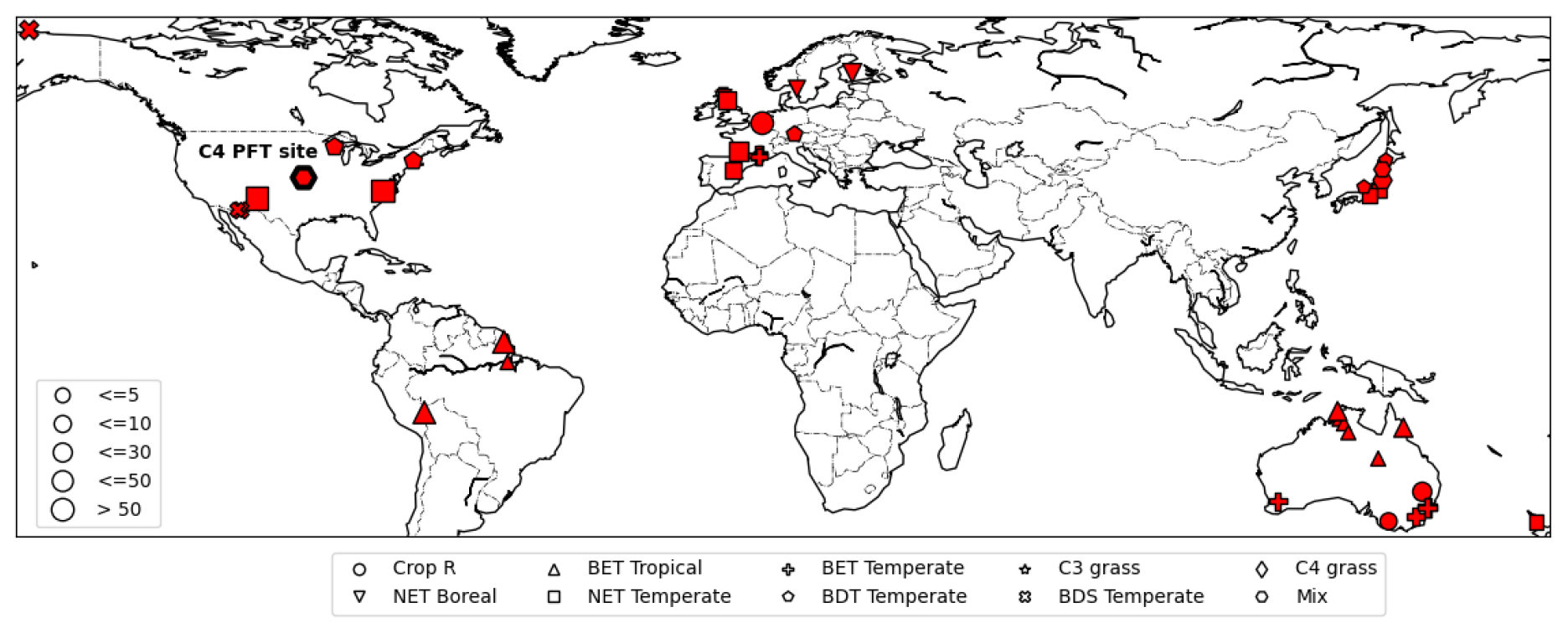
Figure 3 Map of sites available from the leaf gas exchange database (Lin et al., 2015). Different symbols represent different PFTs. The C₄ site is highlighted by a thick-bordered hexagon. The marker sizes represent the quantity of data available for each site (map based on matplotlib basemap; Hunter, 2007).

Lin15 also contained forcing variables, including air temperature (T), leaf temperature (T_v), atmospheric pressure (P_atm), relative humidity (RH), photosynthetic active radiation (φ) and boundary layer conductance (g_b). We used ERA5 to fill in for any missing forcing variables in Lin15. In Eq. (4), P_atm and g_b were used directly from the dataset, while C_a was estimated using observations of the leaf surface CO₂ concentrations, and g_s was calculated using the Medlyn conductance model (Medlyn et al., 2011) as explained in Appendix A.

2.4.2 Static attributes

For β_t calculations, we used data from Hengl and Wheeler (2018) for the soil organic carbon content at different soil depths, where the conventional Van Bemmelen factor of 1.72 was used to convert to soil organic matter (F_om). Data for sand and clay percentages (%sand, %clay) were obtained from Hengl (2018). Both are global datasets available at 250 m resolution at six different soil depths (0, 10, 30, 60, 100, and 200 cm), which describe five soil layers.

2.4.3 CLM4.5 default parameters

CLM4.5 documentation (Oleson et al., 2013) provides reference values for comparison and equations for both target parameters V_c,max25 and B. For V_c,max25, default values corresponding to each PFT (shown in Table 3) are well documented in CLM4.5 (Chap. 8; Table 8.1). Similarly, for parameters B and β_t, their default equations (shown in this work in Appendix B) are provided in the documentation of CLM4.5 as well. We also used other PFT photosynthetic parameters required for β_t computations, such as the soil matric potentials for closed stomata, ψ_c, and open stomata, ψ_o (see Eqs. 8, 10, 12), and the plant root distribution parameters (see Eq. 9).

2.5 Synthetic data and real data experiments

2.5.1 Case 1: synthetic data

In our synthetic experiments, we assumed values for some parameters to generate synthetic photosynthesis rates that could serve as synthetic training data. Then, we estimated those parameters with NNs while keeping other components unmodified. These experiments were intended to verify the plausibility and efficiency of the dPL framework and to verify the identifiability of parameters.

In the first synthetic case, “V_c,max-only”, the δ_psn framework was tested for its ability to accurately retrieve a single PFT-dependent parameter, V_c,max25, using NN_V. We used the suggested values for V_c,max25 from CLM4.5 for different PFTs to calculate the synthetic net photosynthetic rates (synthetic training data). For this case the β_t values were kept constant (equal to one) for all data points, since we intended to test the retrievability of one parameter.

In the second synthetic case, “V_c,max-B”, we tested simultaneously retrieving both V_c,max25 and B, the latter of which varies spatially for different static attributes. For simplicity, we used only the topsoil layer for this case and excluded the influence of the PFT term; therefore we assumed $B_{\mathrm{1}}=\mathrm{0.1}\cdot F_{\mathrm{om},\mathrm{1}}+\mathrm{0.45}\cdot (\mathit{\%}{\mathrm{sand}}_{\mathrm{1}}+\mathit{\%}{\mathrm{clay}}_{\mathrm{1}})$ to generate the synthetic data. The plant wilting factor (w₁) was then calculated using Eq. (12) and was fed into Eq. (9) to compute the soil water stress function (β_t). Since we were using only the topsoil layer, β_t was simplified to (β_t=w₁r₁) with a root distribution value for the topsoil layer (r₁=1). To retrieve B₁, we used NN${}_{B_i}$ (see Eq. 11) but excluded the PFT term since it was not used in synthesizing B₁ values.

For both synthetic runs “V_c,max-only” and “V_c,max-B”, the MLP models were trained concurrently for all PFTs with several data points for each PFT. Moreover, white noise was added to the synthetic values of A_n with a standard deviation of 5 % of the mean value.

2.5.2 Case 2: real data

Once we confirmed that the model passed the test of the synthetic case (correctly retrieving parameter values which were used to generate the data it was given), it was then applied to a real dataset (Lin et al., 2015) using observation data. This tested whether the model, learning from this dataset for many of the PFTs, could find parameters to better describe photosynthesis data than the literature values. There was no ground truth in this case so we tested multiple formulations to better understand the impacts of allowing more or less flexibility in the estimation and role of each parameter.

We tested several formulations to estimate either one (V_c,max25) or two parameters (V_c,max25 and B) at a time. In essence, we compared allowing either one or two of the parameters to be estimated vs. using the default formulation or values from the original model. For V_c,max25, the default values were those defined in CLM4.5, while for β_t, the default equations (Appendix B) were used to obtain its values. Altogether, we trained the following models.

•  

  V_def+B_def: in this case, V_c,max25 took the default values from CLM4.5 and B was calculated using the default equations (Appendix B). This was used as a reference case.

•  

  V_def+B: in this formulation, the default V_c,max25 values from CLM4.5 were used while B was estimated using NN${}_{B_i}$.

•  

  V+B_def: in this formulation, V_c,max25 was estimated using NN_V, while B was calculated using the default equations (Appendix B).

•  

  V+B: in this formulation, we employed both NN_V and NN${}_{B_i}$. They were trained concurrently to see if this interfered with parameter retrieval.

Representing a real case, B_i was estimated for the ith soil layer based on the static attributes for that layer in the four tested model formulations. Thus, B_i varied both horizontally and vertically for each PFT.

Just as in the synthetic case, the MLPs were shared between all sites. All sites were used to calculate one loss function as in typical ML tasks, with the hope of ensuring the wide applicability of the MLPs and leveraging the synergy between all sites (Fang et al., 2022). In this way, we also hoped to identify parameters that generalize well in space and are applicable at large scales.

The MLPs employed had three layers: an input layer, a single hidden layer, and an output layer. To ensure an output value between 0 and 1 for both V_c,max25 and B parameterizations, sigmoid activation functions were used for both hidden and output layers. V_c,max25 was then rescaled to be within a pre-defined range based on literature values of 20 to 150 µmol m⁻² s⁻¹. For the ith soil layer, B_i values were kept between 0 and 1, so with S_i ranging between 0.01 and 1 (see Appendix B), the term $S_i^{-B_i}$ then had a range of 1 to 100. This ensured that the value of ψ_i ranged from ψ_c to ψ_o (see Eq. 10).

The quantity of available data posed a limitation and did not permit an extensive hyperparameter tuning experiment with a train/validation/test split. Hence, we employed a “lazy” trial and error process with hyperparameters (learning rates and hidden size) using 70 % of the data as training data and 30 % as a validation set just to ensure we had a roughly reasonably performing hyperparameter set. We selected a learning rate of 0.045 and a hidden size equal to the number of inputs (nine for NN_V and eight for NN${}_{B_i}$). We kept these same hyperparameters when we ran five-fold cross validation with an 80 % : 20 % train : test ratio. In addition, we found that moderately perturbing the hyperparameters resulted in very little change in the performance (see Appendix C). This design was necessary considering the practical limits of the available data, even though this study already represents a large-sample study in the domain of ecosystem modeling.

Two different tests were performed with respect to data splitting: temporal holdout and randomized cross validation – the former test stresses the models' ability to project into the future, while the latter is the typical experiment run in the literature. Due to the irregularity of measurement dates at each location (as mentioned previously in Sect. 2.4.1), the temporal periods for the training and testing datasets varied by location. In the temporal holdout test, for each PFT in each location, the available dates of measurements were recorded. The oldest 80 % of these dates were used for training and the remaining most recent 20 % were used for testing. The temporal holdout test was run for both synthetic and real data experiments. For the randomized cross validation test, as the name implies, the dataset was randomly split into five folds (groups) and each time the model was trained on four folds (80 % of the data points) and tested on the 5th fold (20 % of the data points). This was done a total of five rounds so that all of the data points were used for testing once. The cross validation test was run only for the real data experiments.

We then compared the values of V_c,max25 learned by the V+B model, trained on all data points, against values of V_c,max25 in other data sources (Kattge et al., 2020; Rogers, 2014), which highlights the variability of these parameters. The TRY database (Kattge et al., 2020) has V_c,max25 values defined for several species which can be aggregated to get unique values for each PFT (Table 3). Moreover, we compared our V_c,max25 values to the ones used in different Earth system models (ESMs; Rogers, 2014) for various PFTs, e.g., the Atmosphere-Vegetation Interaction Model (AVIM; Ji, 1995) and the Biosphere Energy Transfer Hydrology scheme (BETHY; Knorr and Heimann, 2001). The comparison enabled us to determine whether the inversely determined values were on the same order of magnitude as previously employed in the literature, and were physically plausible. We expected our values for different PFTs to be at least partially correlated with the ones used in the literature, as they were meant to represent the same physical quantity. A complete disagreement or a different order of magnitude would suggest that our values may not be physically representative. Partial discrepancies would highlight any knowledge gaps. We did not perform a similar comparison between learned and computed B_i values from default equations since the new shape parameter B_i(soil,PFT) (see Eq. 11) is different from the original one and has a different range (between 0 and 1).

2.6 Statistical metrics

To evaluate different experiments and explore the sensitivity of the results to changing different parameters, we chose four different metrics as shown in Table 1. The four metrics were root mean square error (RMSE), bias, Pearson's correlation (COR), and Nash–Sutcliffe efficiency (NSE). Both RMSE and bias measure how far the model simulations are from the observations (and thus the ideal value is 0); however, RMSE is the standard deviation of all errors while bias is calculated as the average. COR measures the linear relationship between both the simulations and the observations, ranging between −1 and 1. NSE measures the relative magnitude of the residual variance relative to the observed data variance (Nash and Sutcliffe, 1970), and has a perfect score of 1. Table 1 shows the formulations of the four metrics and their possible ranges.

Table 1 Performance metrics used for evaluation and their possible ranges.

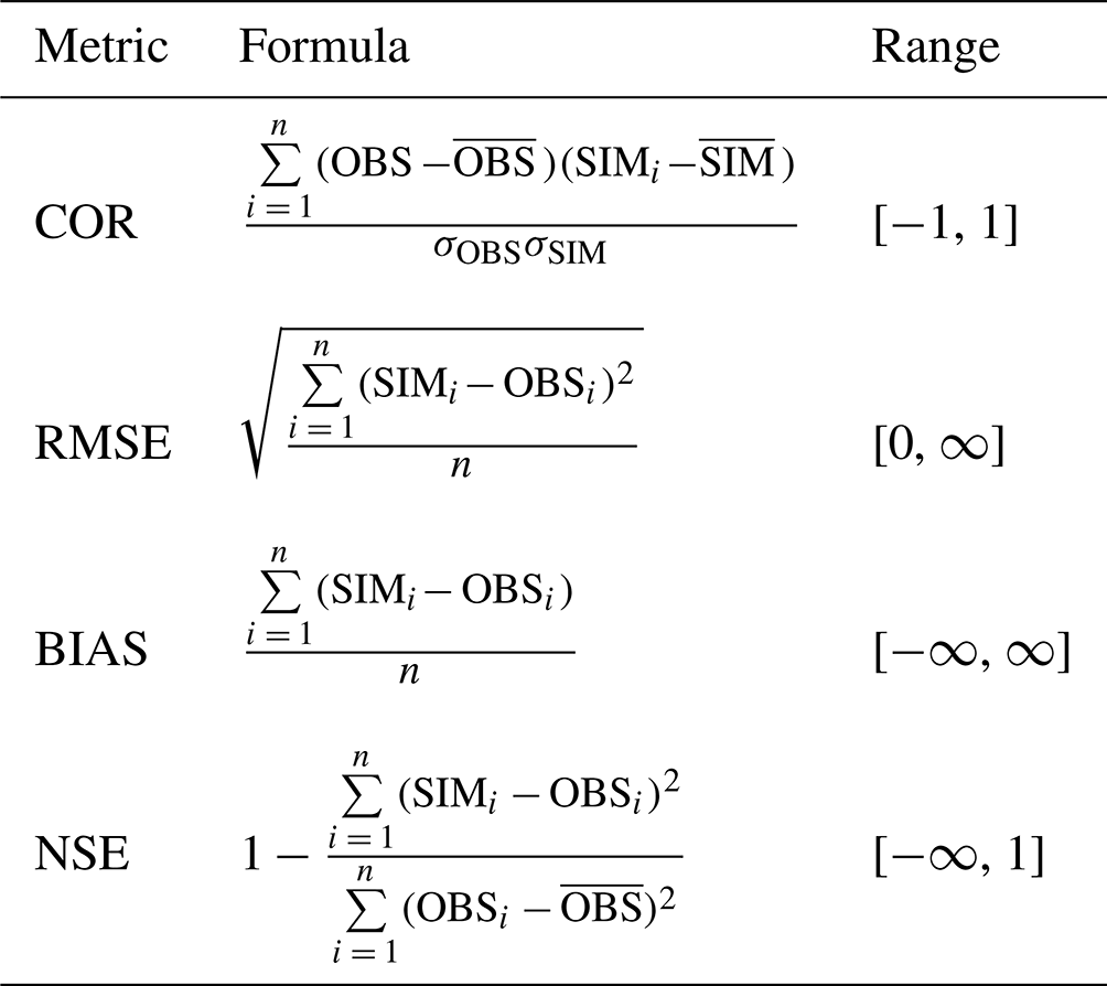
σ refers to the standard deviation, $\stackrel{\mathrm{‾}}{\mathrm{OBS}}$ refers to the mean of the observed values, and $\stackrel{\mathrm{‾}}{\mathrm{SIM}}$ refers to the mean of the simulated values.

3 Results

3.1 Results for synthetic data case

The results of the synthetic experiments showed that our workflow successfully recovered the parameters in both the one-parameter case (“V_c,max-only”, Fig. 4) and the two-parameter case (“V_c,max-B”, Fig. 5). In the one-parameter “V_c,max-only” case, the recovered parameters agreed with the assumed values almost completely for each PFT (Fig. 4a). The model was able to capture the variability in the values of V_c,max25 for different PFTs, where the values ranged from 100.7 µmol m⁻² s⁻¹ for rainfed crops (defined as Crop R in CLM4.5) to around 50 µmol m⁻² s⁻¹ for C₄ grass (Fig. 4a). Moreover, we found nearly complete agreement between the synthetic and recovered net photosynthesis rates (A_n; Fig. 4b). This single-parameter case demonstrated that the dPL framework and the posited formulation $V_{\mathrm{c},\max \mathrm{25}}={\mathrm{NN}}_V\left(\mathrm{PFT}\right)$ were functional, but (as intended) did not show the effects of parameter interactions.

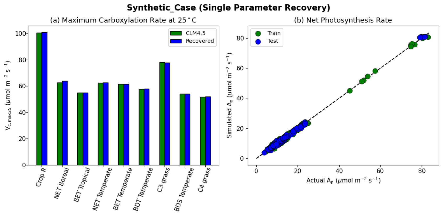
Figure 4 Single parameter recovery for synthetic data. (a) Comparison of modeled parameter values to literature values by PFT. (b) Actual and modeled net photosynthesis rates for training and testing periods (dashed line indicates the ideal 1 : 1 relationship).

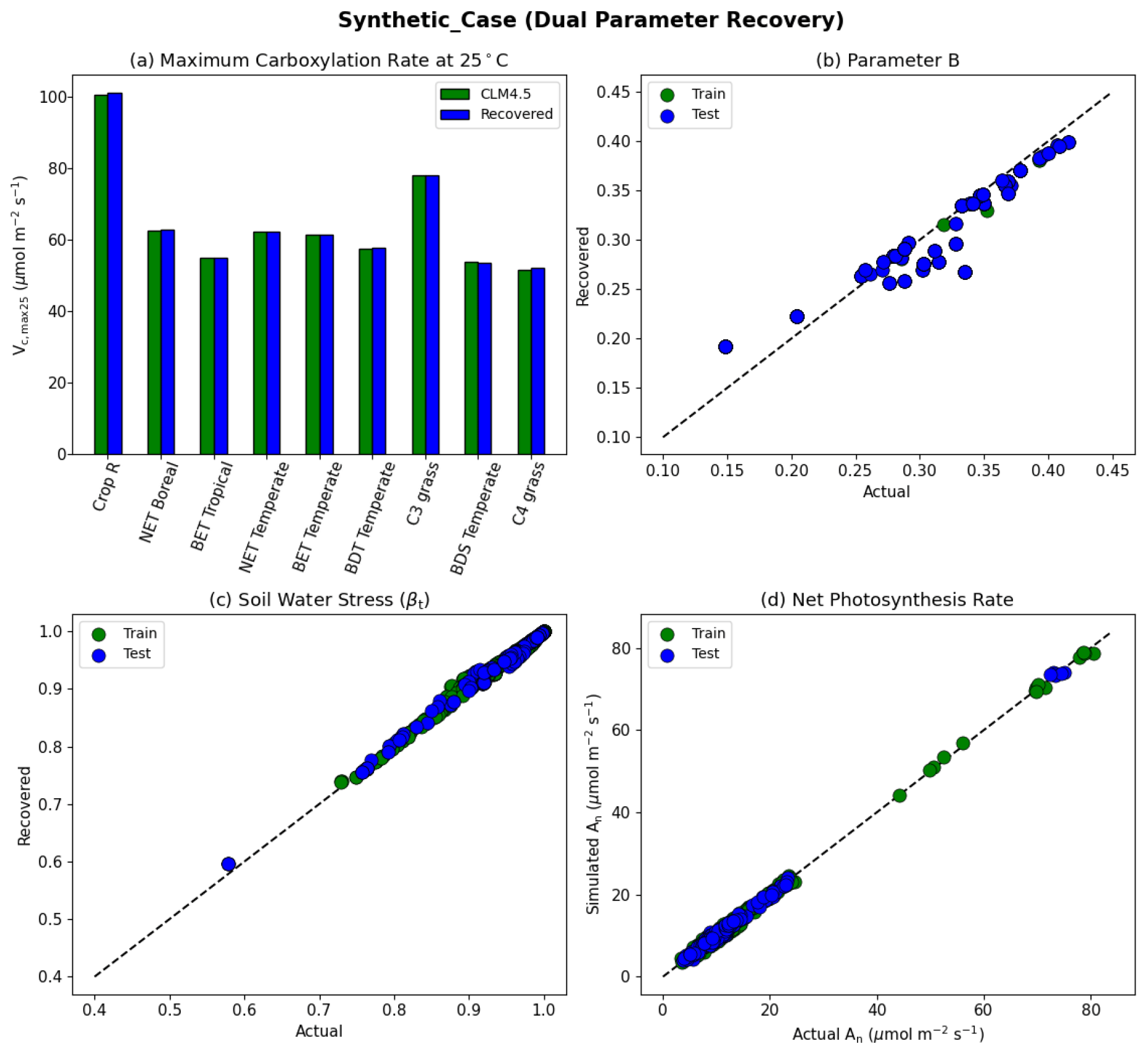
Figure 5 Dual parameter recovery for synthetic data. (a) Comparison of modeled parameter values to literature values by PFT estimated using NN_V. (b) Actual and modeled parameter values for B, estimated using NN${}_{B_i}$. (c) Actual and modeled parameter values for β_t for the topsoil layer. (d) Actual and modeled net photosynthesis rates for training and testing periods. Dashed lines in (b)–(d) indicate the ideal 1 : 1 relationship.

With the dual-parameter case, we found a similarly near-complete recovery for V_c,max25 (Fig. 5a) and a near-complete reproduction of simulated photosynthesis (Fig. 5d). However, we noticed a negligible amount of scattering with β_t (Fig. 5c), and to a larger extent, with B (Fig. 5b). For all experiments, we verified that the training and testing periods were highly consistent (between green and blue points in the scatterplots). The results indicate that the problem formulation allows for sufficient sensitivity of the net photosynthesis rate with respect to PFT-specific V_c,max25 and the soil water constraint. In addition, V_c,max25 and B influence the photosynthesis rate in different ways so that, along with a large dataset with different combinations of moisture conditions and PFTs, they can be identified simultaneously. This forms the basis of the next stage of the work. The soil moisture parameter identifiability was slightly weakened compared to V_c,max25 because there were more equations involved between B and A_n, and some of them had parameters in the exponential operators, e.g., ${\mathit{\psi }}_i={\mathit{\psi }}_{\mathrm{o}}\cdot S_i^{-B_i}$. Mathematically, such a curve can be flat and the gradients can be small in some ranges of S. Mechanistically, A_n can have reduced sensitivity to B under some conditions. Therefore, we do not expect soil properties to be fully identifiable from photosynthesis data, but the general pattern may still be learnable.

3.2 Results for real data case

3.2.1 Comparisons between candidate formulations

In the test cases employing real datasets, the V+B model (employing both NN_V and NN${}_{B_i}$) exhibited obvious advantages over the default photosynthesis module in FATES model and the default parameters, as well as the models that learned only one of the parameters (Table 2). For the temporal holdout test, the default CLM4.5 parameters (V_def+B_def) led to a lower correlation (0.539), a large bias (1.330 µmol m⁻² s⁻¹) and nearly zero NSE (0.001, resulting mainly from the large bias; Table 2a). In particular, the default values appeared to cause an underestimation of the net photosynthetic rate (A_n) for BET Tropical (Fig. 6a, I) and C₃ grass (Fig. 6a, II) but large overestimation for the high-photosynthesis data points of C₄ plants (Fig. 6a, III). After allowing B to be learned (V_def+B), the correlation for testing slightly increased to (0.551), while the bias remained high (0.724 µmol m⁻² s⁻¹); it seems that the learning of water stress alone did not address the bias. On the other hand, when we only allowed V_c,max25 to be estimated (V+B_def), the bias greatly increased (−1.653) and the test NSE was slightly decreased to (0.130). Finally, if we allowed both parameters to be learned (V+B), a decent correlation was obtained (0.757), the bias was the smallest value yet (−0.327 µmol m⁻² s⁻¹), and the test NSE was 0.565, which means the model explained about half of the variance in the observed photosynthesis rate. The remaining error might be attributable to other untuned parameters, processes related to vegetation states which are not considered by the present model. These issues can be potentially further improved in the future using the differentiable modeling paradigm.

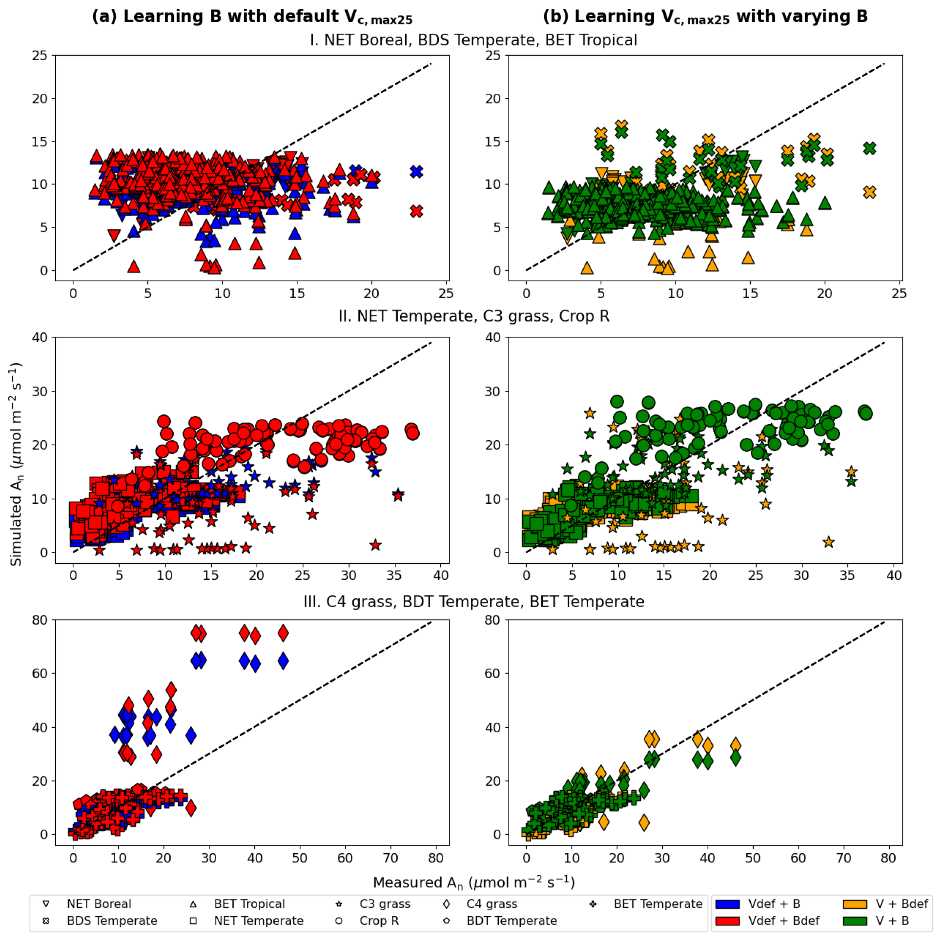
Figure 6 Comparisons of photosynthesis model calibration. Comparing impacts of default and learned parameters by plotting observed vs. simulated A_n (net photosynthetic rate) values calculated using different candidate models (described by which parameter definitions they use). (a) Impact of learning B with default V_c,max25. (b) Impact of learning V_c,max25 with varying B (either learned alongside V in V+B or defined by the default equations in CLM4.5). The colors represent the results from the four different models, the shapes indicate the PFT groups, and the dotted line in each panel indicates the ideal 1 : 1 relationship. Subscript “def” indicates that the variable was calculated using the default definitions in CLM4.5, while no subscript indicates that the parameter was learned using an NN. Scatterplots were created using the test results from each of the five folds of the cross validation test. For better illustration, only three PFTs are placed in a panel, as indicated by the panel titles. Comparing symbols in the same panel gives insights about the role of estimating B, while comparing left and right panels gives insights about the role of estimating V_c,max25.

Table 2 Performance metrics for the candidate models for the Lin15 dataset. In the following, the subscript “def” indicates that the default parameter value from CLM4.5 was used, while parameters without “def” were estimated as an output of a NN (in all cases, V indicates that V_c,max25 was estimated as a function of PFT using NN_V and B indicates estimation using NN${}_{B_i}$). Part (a) shows the temporal holdout test, where the oldest 80 % of data points were used for training and the most recent 20 % were reserved for testing; part (b) shows the cross validation (five-fold) test.

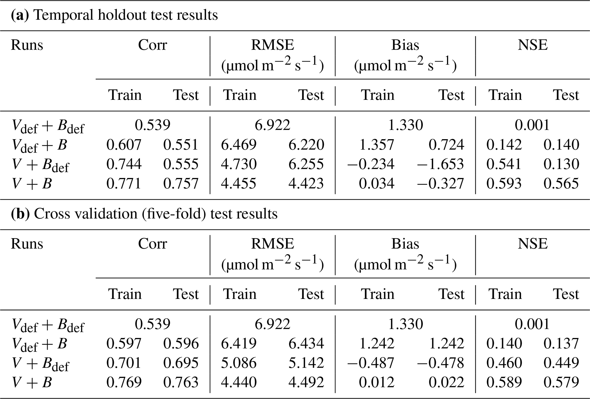
A similar behavior in the performance metrics was observed for the five-fold cross-validation test (see Sect. 2; Table 2b). The cross validation test decreased to a great extent the disparity in the metrics' values between the training and testing datasets (Table 2b). However, contrary to the temporal holdout test, we found a slight improvement in COR (0.596) and NSE (0.137) when B was learned (V_def+B), while a much higher boost was found in the metrics when V_c,max25 was learned (V+B_def). This shows the higher impact of learning V_c,max25 on the simulation of A_n, where the COR and NSE increased to 0.695 and 0.449, respectively, while the bias decreased to −0.478. Similar to the temporal holdout test, the V+B model showed the best metrics in comparison to other models, with the lowest RMSE (4.492) and bias (0.022) values, and the highest COR (0.763) and NSE (0.579) values.

Consistent with the observations of the synthetic experiments, V_c,max25 and B impacted A_n in different ways. When V_c,max25 was not adjusted, the photosynthesis rates simulated for a number of sites in the high A_n range (most of them C₄ plants) had some substantial overestimation, regardless of whether B had learned or default values (Fig. 6a). It was only after the model also learned V_c,max25 that these high biases were reduced (Fig. 6b). Hence, apparently, the learning reduced the V_c,max25 for these sites compared to the default values. In contrast, learning B mainly corrected the low bias for low simulated A_n data points (specifically for BET Tropical, C₃ grass, and C₄ grass; Fig. 6b). A group of sites with underestimations in A_n has been corrected upward (from yellow to green, bottom points in Fig. 6b) due to a correction in the soil parameter B. Apparently, the original parameters overestimated the water stress for these sites. Learning both parameters together was also effective in reducing overestimations and underestimations in the simulated A_n for NET Boreal and BDS Temperate, respectively. Our results suggest the adjustments to both parameters improved the results, but V_c,max25 was more impactful, especially in addressing the bias.

We also noticed the different PFTs benefited differently from the parameter learning. For example, BDS Temperate and Crop R did not benefit much (compare red symbols in Fig. 6a and green symbols in Fig. 6b), BET Tropical and NET Temperate saw moderately improved correlation, while C₃ grass and C₄ grass saw significant improvements in both correlation and bias. These observations indicate the parameters (and thus related processes) tuned here (V_c,max25 and B) have large impacts on C₃ and C₄ grass while other untuned processes, e.g., vegetation growth and nutrient states, may be contributing to the errors with BDS Temperate and Crop R. C₃ plants' improvement is mostly due to learning B, as they are more sensitive to drought in the model, while C₄ plants' improvement is due to learning V_c,max25, as they are more resistant to drought but more sensitive to light in the model.

In addition, our test showed that the framework is moderately impacted by long-term nonstationarity, as the temporal test had worse metrics than the cross-validation test (compare Table 2 part b with a). The absolute value of the bias increased from 0.022 in the cross validation test to 0.327 in the temporal test. This suggests that the current model (and perhaps the training data) still has some limitations with representing long-term changes. Possible reasons may include CO₂ fertilization and its impact on water use efficiency or differences in the state of plants, as this factor is not included in our present parameterization. In the future, these issues could be addressed by assembling a more long-term training dataset (the Lin15 dataset has data ranging from 1991 to 2013), as well as improving the parameterization and physics of the model.

3.2.2 Recovered parameters

Even though we did not prescribe the values of V_c,max25, the training on the dataset converged to parameter values that were partially correlated with, yet still substantially different from, the literature values, and were on the same order of magnitude (Fig. 7). The default V_c,max25 values came from in situ measurements at a limited number of sites, while our values came from learning from a moderately large dataset (essentially an inversion process limited to the model structure). The fact that they agreed with each other in the main pattern suggests both have merit, and that the learning process captured fundamental physics. The upper half of Fig. 7b saw a high correlation, but V_c,max25 values for the V+B model were uniformly higher than the CLM4.5 defaults, especially for the NET Boreal PFT. The correlation was lower toward the lower half of Fig. 7b (where V_c,max25 from CLM4.5 was lower than 65 µmol m⁻² s⁻¹) – the learned V_c,max25 had a larger variability. In particular, the learned V_c,max25 (V+B) for C₄ grass is much lower than the default, which could be attributed to species-level variability and the fact that the dataset contains very limited sites with C₄ plants. Hence, we do not argue that the values learned here would be applicable globally to other C₄ grasses. It seems that the inter-PFT variability in V_c,max25 was previously underrepresented by the CLM4.5 default parameter values (BET Tropical, BET Temperate, BDS Temperate, C₄ grass), and the learning process used here enhanced the variability. Moreover, we note that for either Crop R, BET Tropical, BET/BDT Temperate, or C₄ grass, the influence of learning B on V_c,max25 was mostly small (V_c,max25 from V+B and V+B_def models were mostly similar), and thus the interactions between these two parameters were not significant. The overall results showcase the ability of the algorithm to adapt to data and reveal parameter interactions.

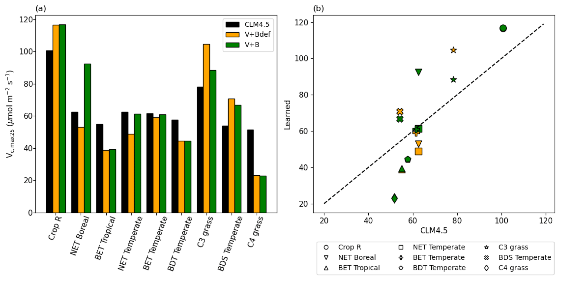
Figure 7 Parameter recovery for real data. (a) Comparison of modeled parameter values to literature values of V_c,max25 by PFT. (b) Actual and modeled V_c,max25 values plotted by PFT (dashed line indicates the 1 : 1 ideal relationship). In this figure, both “V+B_def” and “V+B” models were trained using the whole dataset.

In our interpretation, the learned values represent a more “fine-tuned” version of the literature V_c,max25 values, with the interference from soil water stress disentangled. The magnitude and ranking for PFTs remained similar to the literature values, but the results were improved in different ways for different PFTs. The V+B model obtained lower V_c,max25 for C₄ grass, addressing the significant overestimation bias for these sites, which we noted in Fig. 6a, III. Due to their different photosynthesis pathway, C₄ plants have the lowest learned V_c,max25, but overall the highest net photosynthesis rates, which were not heavily influenced by the choice of the B parameter. For C₃ grass, V+B only slightly increased V_c,max25 compared to the default CLM4.5 values, which addressed the notable low bias in Fig. 6b, II. The default soil parameterization for C₃ grass sites seemed somewhat deficient as soil water stress accounted for the other parts of variance in net photosynthesis, as demonstrated by the comparison between V+B and V+B_def models in Figs. 6b-II and 7b for C₃ grass.

We compared our learned V_c,max25 values (Table 3 and Fig. 8) with values from other ESMs and with some observatory values in the TRY database (Kattge et al., 2020; Rogers, 2014). The learned V_c,max25 values are higher than those of the TRY database for most PFT classes except for BDT Temperate and BDS Temperate; however, they are within the range of values used in other ESMs except for relatively higher estimations for Crop R, NET Boreal, and C₃ grass. On the scale of ESMs, several values for V_c,max25 are adopted by those models. We computed the correlation coefficient between our learned V_c,max25 values and reference values from other ESMs and the TRY database, finding high correlations (except for AVIM) between the learned and reference V_c,max25 values for CLM4.5 (0.844), BETHY (0.900), and the TRY database (0.699). For instance, V_c,max25 for C₄ grass is 25 and 20 (µmol m⁻² s⁻¹) in AVIM and BETHY, respectively (Table 3). These values agree with the learned V_c,max25 of the V+B model of 22.90 (µmol m⁻² s⁻¹), whereas much higher values were found to be adopted for C₄ grass, with 60 (µmol m⁻² s⁻¹) being used in the biogeochemical cycles model BiomeBGC as reported in Rogers (2014) and 51.6 (µmol m⁻² s⁻¹) in CLM4.5. V_c,max25 from the V+B model and TRY database are similar for BET Tropical and BDT Temperate. For BDS Temperate, the learned V_c,max25 was lower than that in TRY by ∼ 20 (µmol m⁻² s⁻¹), but similar values were used by BETHY and lower values were used by AVIM. For Crop R, NET Boreal, NET Temperate, and BET Temperate, the learned V_c,max25 values were all ∼ 20–30 (µmol m⁻² s⁻¹) higher than those of the TRY database, but (except for NET Boreal) similar values have been used in AVIM or BETHY. Both the learned (V+B) and the observed (TRY database) V_c,max25 values show a similar pattern to the lowest V_c,max25 for BET Tropical and a high value assigned for Crop R.

Table 3 V_c,max25 simulated by the V+B model versus observed values from the TRY database (with partial overlap in species with the Lin15 dataset – the percentage of overlap is provided in the table), and used in different ESMs such as CLM4.5, AVIM, and BETHY.

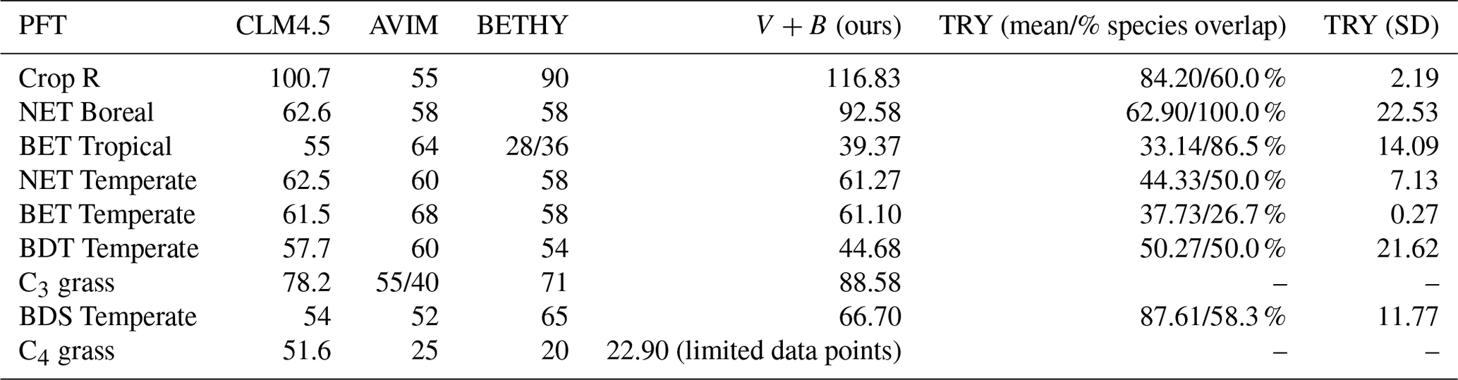
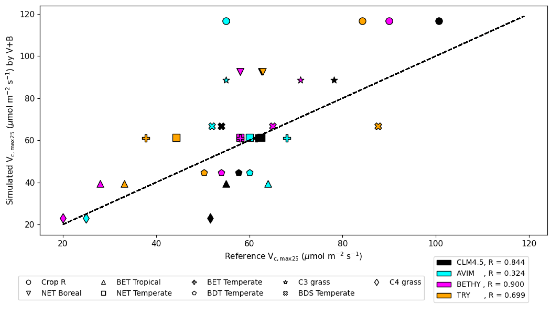
Figure 8 The correlation between the V_c,max25 values estimated by the V+B model on the y axis versus V_c,max25 values from CLM4.5 (black markers), AVIM (cyan markers), BETHY (magenta markers), and the TRY database (orange markers). Different marker shapes represent different PFTs, while different colors represent different reference sources for V_c,max25 per PFT. For the TRY database, we do not have values for C₃ grass and C₄ grass due to the lack of overlap in species between the TRY database and our dataset for those two PFTs. The dashed line indicates a 1 : 1 relationship.

4 Discussion

As an initial exploration of the potential of the emerging differentiable computing paradigm (a genre of physics-informed ML; Shen et al., 2023) for applications in ecosystem modeling, our work showed promise but also had many limitations, as the goal was not to produce the best-performing photosynthetic model. We restricted our parameter sets to be dependent on PFT, whereas it is known that within-PFT variation can be significant, and parameters could also be determined on the trait level as well as by multiple environmental factors. Our model did not consider the effects of memory (e.g., rainfall in previous days) or the state of the vegetation (e.g., carbon stored in the canopy or carbon : nitrogen ratios in the canopy). The soil moisture data comes from the ERA5 dataset, which, based on comparisons to in situ data, would be outperformed by ML-based soil moisture predictions (Fang et al., 2017; Liu et al., 2022, 2023), but we used it due to its seamless global coverage and availability for multiple soil depths. This work also only modified the parameterization scheme and did not learn model structures. Recently, development in differentiable hydrologic models has allowed for learning parts of the model using NNs (Feng et al., 2022a, b). In summary, we believe there is still much room for improving model quality, but at some point we will likely run into the limits of measurements (aleatoric uncertainty) or data availability (epistemic uncertainty; Hüllermeier and Waegeman, 2021). Future effort can harness deep networks to establish reference levels as a measure of the data uncertainty (Feng et al., 2022a).

This work appears to be the first evaluation of the Lin15 dataset, and, as such, it establishes a reference level to which future studies can compare. The current dataset may still have limitations in that the number of sites for C₄ plants is small and in that it does not allow for ample testing. Some geoscientific domains have well-known benchmark datasets, e.g., the CAMELS dataset in hydrology (Feng et al., 2020). Having such a common (and hopefully large) benchmark dataset allows better model structures to be rapidly discovered and is highly beneficial to the growth of the community (Shen et al., 2018). Related to the limits of measurement errors discussed above, multiple deep-learning-based studies have explored the approximate data error limit (or best achievable model) of CAMELS and that knowledge has been appreciated by the community (Feng et al., 2021). Moreover, deep learning methods benefit from data synergy effects (Fang et al., 2022), where more sites and more diverse data lead to a more robust model and better performance for each site.

Although applying the dPL framework improved the parameters to an extent, the model still has similar structural limitations as other Farquhar-type models. We did not test the model's ability to capture the seasonality of the net photosynthetic rate due the limited site-level temporal data. The seasonal behavior of the model is expected to be similar to other Farquhar models as here we only learned static parameters. Further improvement likely will need to consider vegetation growth. Also, this study did not cover spatial generalization since we do not present results for spatial tests nor is it based on site-level comparison. Improving spatial generalization may require further changes in the model or dynamical parameters or the use of other error mitigation approaches (Feng et al., 2021, 2022b; Ma et al., 2021). This was not within the scope of this study; however, it will be considered for future work.

We would like to highlight that such parameterizations are suitable to the target and forcing datasets used in training (which is still the most representative accessible dataset) and are related to the PBM employed. The dataset may have limitations related to the consistency of the measurement approach, and there may be errors in the forcing data or imperfections in model structure. The model performance may also vary based on the different forcing data and inputs used.

5 Conclusions

In this study, we proposed a novel differentiable ecosystem modeling framework that uses NNs as a parameterization scheme to support a process-based ecosystem model (FATES). Training coupled NNs was not previously possible without differentiable programming, and it allows us to approximate complex a priori unknown mapping relationships between PFTs, landscape characteristics, and physical parameters. The photosynthesis module was treated as a system of nonlinear equations, and, like other such systems, could be solved efficiently and in a massively parallel fashion on GPUs by our differentiable framework. V_c,max25 and a soil water parameter (B) could be simultaneously identified in our synthetic experiments, because they played different roles in the model.

Compared to purely data-driven ML approaches, the differentiable programming framework provides physically meaningful variables and can be used to learn relationships from big data. Via training on a global dataset, we found V_c,max25 values for global sites that correlate with the values in the literature but produce more accurate net photosynthesis rates. It is noteworthy that these values were identified without any supervision from experts other than the preparation of the training dataset and the model. We conclude that V_c,max25 has a larger impact on photosynthesis than the soil water stress parameter, but both can be useful in tuning model responses, with varied impacts on different plants, and their default values were not optimal. Not only is differentiable modeling able to improve simulation quality and provide model parameterization, it also allows us to modify model structure and ask questions regarding unclear parts of the model in the future. There is significant room for this framework to improve and expand to other ecosystem modeling applications.

Appendix A: The system of nonlinear equations

The FATES photosynthesis module is based on the classical Farquhar model for C₃ plants (Farquhar et al., 1980), which calculates the photosynthetic rate based on carbon fluxes under different limitations. For C₄ plants, it uses the Collatz model (Collatz et al., 1992). Both models assume that the gross photosynthetic rate is affected by the maximum rate of carboxylation and is limited by the concentration of Rubisco (A_c; see Eq. A1), light and electron transport (A_j; see Eq. A2), and the concentration of PEP carboxylase enzyme in C₄ plants (A_p; see Eq. A3). A_c,A_j, and A_p are calculated as

$$\begin{array}{}\text{(A1)}& {\displaystyle }{A}_{\mathrm{c}}=\left\{\begin{array}{ll}\frac{V_{\mathrm{c},\max }\times \left(C_{\mathrm{i}}-{\mathrm{\Gamma }}_{\ast }\right)}{C_{\mathrm{i}}+K_{\mathrm{c}}\left(\mathrm{1}+\frac{O_i}{K_{\mathrm{o}}}\right)}& \mathrm{for}{\mathrm{C}}_{\mathrm{3}}\mathrm{plants}\\ V_{\mathrm{c},\max }& \mathrm{for}{\mathrm{C}}_{\mathrm{4}}\mathrm{plants}\end{array}\right\},\text{(A2)}& {\displaystyle }{A}_{\mathrm{j}}=\left\{\begin{array}{ll}\frac{J_x\times \left(C_{\mathrm{i}}-{\mathrm{\Gamma }}_{\ast }\right)}{\mathrm{4}{C}_{\mathrm{i}}+\mathrm{8}{\mathrm{\Gamma }}_{\ast }}& \mathrm{for}{\mathrm{C}}_{\mathrm{3}}\mathrm{plants}\\ \mathit{\alpha }\left(\mathrm{4.6}\mathit{\phi }\right)& \mathrm{for}{\mathrm{C}}_{\mathrm{4}}\mathrm{plants}\end{array}\right\},\text{(A3)}& {\displaystyle }{A}_{\mathrm{P}}=\left\{\begin{array}{ll}{K}_p\frac{C_{\mathrm{i}}}{P_{\mathrm{atm}}}& \mathrm{for}{\mathrm{C}}_{\mathrm{4}}\mathrm{plants}\end{array}\right\},\end{array}$$

where V_c,max is the maximum carboxylation rate, C_i is the intercellular leaf CO₂ pressure (nonlinear system output), Γ_∗ is the CO₂ compensation point, K_c and K_o are the Michaelis–Menten constants, O_i is the O₂ partial pressure (calculated as 20 % of the atmospheric pressure), J_x is the electron transport rate (see Eqs. A4 and A5), α is the quantum efficiency (0.05 mol CO₂ mol⁻¹ photon), φ is the photosynthetically active radiation (available in Lin15), K_p is the initial slope of C₄ CO₂ response curve, and P_atm is the atmospheric pressure (available in Lin15).

Γ_∗, K_c, and K_o are the scaled parameters based on leaf temperature (T_v) calculated using their standardized values at 25 ^∘C which are ${\mathrm{\Gamma }}_{\ast \mathrm{25}}=\mathrm{42.75}\times {\mathrm{10}}^{-\mathrm{6}}{P}_{\mathrm{atm}}$, $K_{\mathrm{c},\mathrm{25}}=\mathrm{404.9}\times {\mathrm{10}}^{-\mathrm{6}}{P}_{\mathrm{atm}}$, and $K_{\mathrm{o},\mathrm{25}}=\mathrm{278.4}\times {\mathrm{10}}^{-\mathrm{3}}{P}_{\mathrm{atm}}$, multiplied by the temperature response functions defined in chapter 9.0 in CLM5.0 (Lawrence et al., 2019).

J_x is given by the minimum root of the following quadratic equation:

$$\begin{array}{}\text{(A4)}& {\mathit{\theta }}_{\mathrm{PSII}}{J}_x^{\mathrm{2}}-\left(I_{\mathrm{PSII}}+J_{\max }\right)J_x+I_{\mathrm{PSII}}{J}_{\max }=\mathrm{0},\end{array}$$

where J_max is the maximum electron transport rate, θ_PSII is an empirical curvature for the electron transport rate (0.7) and I_PSII is the light utilized in electron transport calculated using a quantum yield parameter (Φ_PSII=0.85) as

$$\begin{array}{}\text{(A5)}& I_{\mathrm{PSII}}=\mathrm{0.5}{\mathrm{\Phi }}_{\mathrm{PSII}}\left(\mathrm{4.6}\mathit{\phi }\right).\end{array}$$

The three biophysical rates V_c,max, J_max, and K_p along with the plant respiration rate (R_d), adjusted for T_v, are calculated using their standardized values at 25 ^∘C multiplied by temperature response functions defined in Chap. 9.0 in CLM5.0 (Lawrence et al., 2019). V_c,max is also adjusted for the soil water availability by multiplying it with the soil water stress function (β_t).

In our case, V_c,max25 is either the default value provided in CLM4.5 or it is learned by an NN, which then is used to calculate other standardized biophysical rates as

$$\begin{array}{}\text{(A6)}& {\displaystyle }{J}_{\max \mathrm{25}}=\mathrm{1.67}{V}_{\mathrm{c},\max \mathrm{25}},\text{(A7)}& {\displaystyle }{R}_{d\mathrm{25}}=\left\{\begin{array}{ll}\mathrm{0.015}{V}_{\mathrm{c},\max \mathrm{25}}& \mathrm{for}{\mathrm{C}}_{\mathrm{3}}\mathrm{plants}\\ \mathrm{0.025}{V}_{\mathrm{c},\max \mathrm{25}}& \mathrm{for}{\mathrm{C}}_{\mathrm{4}}\mathrm{plants}\end{array}\right\},\text{(A8)}& {\displaystyle }{K}_{p\mathrm{25}}=\left\{\begin{array}{ll}\mathrm{20}\mathrm{000}{V}_{\mathrm{c},\max \mathrm{25}}& \mathrm{for}{\mathrm{C}}_{\mathrm{4}}\mathrm{plants}\end{array}\right\}.\end{array}$$

The gross photosynthetic rate (A) is then calculated by solving for the minimum root of the quadratic equations:

$$\begin{array}{}\text{(A9)}& {\displaystyle }{\mathit{\theta }}_{\mathrm{cj}}{A}_{\mathrm{i}}^{\mathrm{2}}-\left(A_{\mathrm{c}}+A_{\mathrm{j}}\right)A_{\mathrm{i}}+A_{\mathrm{c}}{A}_{\mathrm{j}}=\mathrm{0},\text{(A10)}& {\displaystyle }{\mathit{\theta }}_{\mathrm{ip}}{A}^{\mathrm{2}}-\left(A_{\mathrm{i}}+A_{\mathrm{p}}\right)A+A_{\mathrm{i}}{A}_{\mathrm{p}}=\mathrm{0},\end{array}$$

where A_i is an intermediate co-limited photosynthetic rate calculated using the empirical curvature parameter (θ_cj=0.999). Using A_i, A_p, and the empirical curvature parameter (θ_ip=0.999), the gross rate (A) is given by the smaller root of Eq. (A10). The net photosynthetic rate (A_n) is

$$\begin{array}{}\text{(A11)}& A_{\mathrm{n}}=A-R_d.\end{array}$$

Then using A_n, the CO₂ partial pressure at the leaf surface (C_s) is calculated as

$$\begin{array}{}\text{(A12)}& C_{\mathrm{s}}=C_{\mathrm{a}}-{\displaystyle \frac{\mathrm{1.4}{P}_{\mathrm{atm}}{A}_{\mathrm{n}}}{g_{\mathrm{b}}}}\ge \mathrm{1.0}\times {\mathrm{10}}^{-\mathrm{6}},\end{array}$$

where C_a is CO₂ partial pressure near the leaf surface (estimated using observations of the leaf surface CO₂ concentrations in Lin15) and g_b is the leaf boundary layer conductance, which was available in Lin15 for some sites and the missing values were filled using the mean g_b of the whole dataset. The stomatal conductance (g_s) is then given by the maximum root of the quadratic equation:

$$\begin{array}{}\text{(A13)}& g_{\mathrm{s}}^{\mathrm{2}}+b{g}_{\mathrm{s}}+c=\mathrm{0},\end{array}$$

where b, c, and d are functions in some PFT-dependent parameters:

$$\begin{array}{}\text{(A14)}& {\displaystyle }b=-\left(\mathrm{2}(g_{\mathrm{o}}+d)+{\displaystyle \frac{{\left(g_{\mathrm{1}}d\right)}^{\mathrm{2}}}{g_{\mathrm{b}}\times \mathrm{vpd}}}\right),\text{(A15)}& {\displaystyle }c=g_{\mathrm{o}}^{\mathrm{2}}+\left(\mathrm{2}{g}_{\mathrm{o}}+d\left(\mathrm{1}-{\displaystyle \frac{g_{\mathrm{1}}^{\mathrm{2}}}{\mathrm{vpd}}}\right)\right)d,\text{(A16)}& {\displaystyle }d={\displaystyle \frac{\mathrm{1.6}{A}_{\mathrm{n}}}{C_{\mathrm{s}}/P_{\mathrm{atm}}}}.\end{array}$$

g_o, the water stressed minimum stomatal conductance, is calculated as the multiplication of β_t and the unstressed minimum stomatal conductance (10 000 µmol m⁻² s⁻¹ for C₃, 40 000 µmol m⁻² s⁻¹ for C₄). g₁, the slope of the Medlyn stomatal conductance model (Medlyn et al., 2011), is a PFT-specific parameter defined in CLM5.0 (Lawrence et al., 2019). vpd, the vapor pressure deficit, was available in Lin15. Finally, C_i, is related to A_n using C_a, P_atm, g_s, and g_b as the following:

$$\begin{array}{}\text{(A17)}& C_{\mathrm{i}}=C_{\mathrm{a}}-A_{\mathrm{n}}{P}_{\mathrm{atm}}{\displaystyle \frac{(\mathrm{1.4}{g}_{\mathrm{s}}+\mathrm{1.6}{g}_{\mathrm{b}})}{(g_{\mathrm{s}}\times g_{\mathrm{b}})}}.\end{array}$$

Appendix B: Computations of btran (β_t) in CLM4.5

β_t is calculated by aggregating the plant wilting factor (w_i) and plant root distribution (r_i) across different soil different layers as

$$\begin{array}{}\text{(B1)}& {\mathit{\beta }}_{\mathrm{t}}=\sum _i{w}_i{r}_i.\end{array}$$

The plant wilting factor (w_i) for soil layer i is mainly dependent on the soil water potential ψ_i and other PFT-dependent parameters such as the soil matric potentials for closed stomata ψ_c and open stomata ψ_o, which represent the soil water potentials when stomata are fully closed and fully open, respectively. The factor w_i is also dependent on other factors like the temperature of the soil layer (T_i) relative to the freezing temperature (T_f), the volumetric liquid water content (θ_liq,i) and volumetric ice (θ_ice,i) content, and the volumetric water content at saturation (θ_sat,i).

$$\begin{array}{}\text{(B2)}& w_i=\left\{\begin{array}{l}\frac{{\mathit{\psi }}_{\mathrm{c}}-{\mathit{\psi }}_i}{{\mathit{\psi }}_{\mathrm{c}}-{\mathit{\psi }}_{\mathrm{o}}}\left[\frac{{\mathit{\theta }}_{\mathrm{sat},i}-{\mathit{\theta }}_{\mathrm{ice},i}}{{\mathit{\theta }}_{\mathrm{sat},i}}\right]\le \mathrm{1};\\ T_i>T_{\mathrm{f}}-\mathrm{2}\mathrm{and}{\mathit{\theta }}_{\mathrm{liq},i}>\mathrm{0}\\ \\ \mathrm{0};\\ T_i\le T_{\mathrm{f}}-\mathrm{2}\mathrm{or}{\mathit{\theta }}_{\mathrm{liq},i}\le \mathrm{0}\end{array}\right\}.\end{array}$$

The soil matric potential ψ_i is calculated using a power-law formulation:

$$\begin{array}{}\text{(B3)}& {\mathit{\psi }}_i={\mathit{\psi }}_{\mathrm{sat},i}\times S_i^{-B_i}\ge {\mathit{\psi }}_{\mathrm{c}},\end{array}$$

where ψ_sat,i is the saturated soil matric potential, S_i is the soil wetness, and B_i is the Clapp–Hornberger parameter, all defined for a specific soil layer (i). Different soil attributes such as percentages of sand (%sand_i) and clay (%clay_i), fraction of organic matter (F_om,i), and soil moisture (θ_liq,i) are used in computing ψ_sat,i, S_i, and B_i. ψ_sat,i is calculated as

$$\begin{array}{}\text{(B4)}& {\mathit{\psi }}_{\mathrm{sat},i}=\left(\mathrm{1}-F_{\mathrm{om},i}\right)\times {\mathit{\psi }}_{\mathrm{sat},\min ,i}+F_{\mathrm{om},i}\times {\mathit{\psi }}_{\mathrm{sat},\mathrm{om}},\end{array}$$

where ψ_sat,om is the saturated organic matter matric potential (−10.3 mm; Letts et al., 2000) and ${\mathit{\psi }}_{\mathrm{sat},\min ,i}$ is the saturated mineral soil matric potential calculated using %sand_i as

$$\begin{array}{}\text{(B5)}& {\mathit{\psi }}_{\mathrm{sat},\min ,i}=-\mathrm{10.0}\times {\mathrm{10}}^{\mathrm{1.88}-\mathrm{0.0131}\times (\mathit{\%}\mathrm{sand}{)}_i}.\end{array}$$

The soil wetness (S_i) is calculated using the volumetric contents θ_liq,i, θ_ice,i, and θ_sat,i as

$$\begin{array}{}\text{(B6)}& S_i={\displaystyle \frac{{\mathit{\theta }}_{\mathrm{liq},i}}{{\mathit{\theta }}_{\mathrm{sat},i}-{\mathit{\theta }}_{\mathrm{ice},i}}},\mathrm{0.01}\le S_i\le \mathrm{1},\end{array}$$

where θ_sat,i for a soil layer is

$$\begin{array}{}\text{(B7)}& {\mathit{\theta }}_{\mathrm{sat},i}=\left(\mathrm{1}-F_{\mathrm{om},i}\right)\times {\mathit{\theta }}_{\mathrm{sat},\min ,i}+F_{\mathrm{om},i}\times {\mathit{\theta }}_{\mathrm{sat},\mathrm{om}}.\end{array}$$

θ_sat,om is the porosity of the organic matter (0.9; Letts et al., 2000; Farouki, 1981), while the porosity of the mineral soil (θ_sat,min) using %sand is

$$\begin{array}{}\text{(B8)}& {\mathit{\theta }}_{\mathrm{sat},\min ,i}=\mathrm{0.489}-\mathrm{0.00126}\times (\mathit{\%}\mathrm{sand}{)}_i.\end{array}$$

Similar to ψ_sat,i and θ_sat,i (see Eqs. B4 and B7), the parameter B_i is calculated as

$$\begin{array}{}\text{(B9)}& B_i=\left(\mathrm{1}-F_{\mathrm{om},i}\right)\times B_{\min ,i}+F_{\mathrm{om},i}\times B_{\mathrm{om}},\end{array}$$

where B_om is the parameter for organic matter (2.7; Letts et al., 2000), while $B_{min,i}$, the parameter for mineral soil, is

$$\begin{array}{}\text{(B10)}& B_{\min ,i}=\mathrm{2.91}+\mathrm{0.159}\times (\mathit{\%}\mathrm{clay}{)}_i.\end{array}$$

Appendix C

Table C1 V+B model formulation performance for different sizes of NN${}_{B_i}$ [input size, hidden size, output size] with a 80 % : 20 % train : test split ratio.

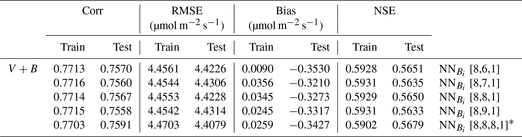
^* In the last experiment we used two hidden layers (i.e., NN${}_{B_i}$ [input size, hidden layer₁ size, hidden layer₂ size, output size]).