Quantifying vegetation indices using terrestrial laser scanning: methodological complexities and ecological insights from a Mediterranean forest

Accurate measurement of vegetation density metrics including plant, wood and leaf area indices (PAI, WAI and LAI) is key to monitoring and modelling carbon storage and uptake in forests. Traditional passive sensor approaches, such as digital hemispherical photography (DHP), cannot separate leaf and wood material, nor individual trees, and require many assumptions in processing. Terrestrial laser scanning (TLS) data offer new opportunities to improve understanding of tree and canopy structure. Multiple methods have been developed to derive PAI and LAI from TLS data, but there is little consensus on the best approach, nor are methods benchmarked as standard.

Using TLS data collected in 33 plots containing 2472 trees of 5 species in Mediterranean forests, we compare three TLS methods (lidar pulse, 2D intensity image and voxel-based) to derive PAI and compare with co-located DHP. We then separate leaf and wood in individual tree point clouds to calculate the ratio of wood to total plant area (α), a metric to correct for non-photosynthetic material in LAI estimates. We use individual tree TLS point clouds to estimate how α varies with species, tree height and stand density.

We find the lidar pulse method agrees most closely with DHP, but it is limited to single-scan data, so it cannot determine individual tree properties, including α. The voxel-based method shows promise for ecological studies as it can be applied to individual tree point clouds. Using the voxel-based method, we show that species explain some variation in α; however, height and plot density were better predictors.

Our findings highlight the value of TLS data to improve fundamental understanding of tree form and function as well as the importance of rigorous testing of TLS data processing methods at a time when new approaches are being rapidly developed. New algorithms need to be compared against traditional methods and existing algorithms, using common reference data. Whilst promising, our results show that metrics derived from TLS data are not yet reliably calibrated and validated to the extent they are ready to replace traditional approaches for large-scale monitoring of PAI and LAI.

1 Introduction

Leaf area index (LAI), defined as half the amount of green leaf area per unit ground area (Chen and Black, 1992), determines global evapotranspiration, phenological patterns and canopy photosynthesis and is therefore an essential climate variable (ECV), as well as a key input in dynamic global vegetation models (Sea et al., 2011; Weiss et al., 2004). Accurate measurements of leaf, wood and plant area indices (LAI, WAI and PAI) have historically been derived from labour-intensive destructive sampling (Baret et al., 2013; Jonckheere et al., 2004), so over large spatial or temporal scales these can only be measured indirectly, typically with remote sensing. Large-scale remote sensing, using spaceborne and airborne instruments, has been widely used to estimate LAI over large areas (Pfeifer et al., 2012), but it requires calibration and validation using in situ measurements to constrain information retrieval (Calders et al., 2018). Non-destructive in situ vegetation index estimates have historically been made by measuring light transmission below the canopy and using simplifying assumptions about canopy structure to estimate the amount of intercepting material (e.g. Beer–Lambert's law; Monsi and Saeki, 1953). The most common method, digital hemispherical photography (DHP; Fig. 1a), requires both model assumptions and subjective user choices during data acquisition and processing in order to estimate both PAI and LAI (Breda, 2003). DHP images are processed by separating sky from canopy, but not photosynthetic from non-photosynthetic vegetative material, so additional assumptions are needed to calculate either LAI or WAI (Jonckheere et al., 2004; Pfeifer et al., 2012). Separation of LAI from PAI can be achieved by removing or masking branches and stems from hemispherical images (e.g. Sea et al., 2011; Woodgate et al., 2016), but it is not reliable when leaves are occluded by woody components (Hardwick et al., 2015). An alternative approach is to take separate DHP measurements in both leaf on and leaf off conditions and derive empirical wood-to-plant ratios (WAI / PAI, α) (Leblanc and Chen, 2001), but this is not always practical, for example in evergreen forests. The difficulty of separation means that studies often omit correcting for the effect of WAI on optical PAI measurements altogether (Woodgate et al., 2016), but since woody components in the forest canopy can account for more than 30 % of PAI (Ma et al., 2016) this can introduce overestimation. Further, although DHP estimates of LAI or PAI are valuable both for ecosystem monitoring and developing satellite LAI products (Hardwick et al., 2015; Pfeifer et al., 2012), they are limited to sampling only at a neighbourhood or plot level (Weiss et al., 2004) and cannot be used to measure individual tree LAI except for open grown trees (Béland et al., 2014).

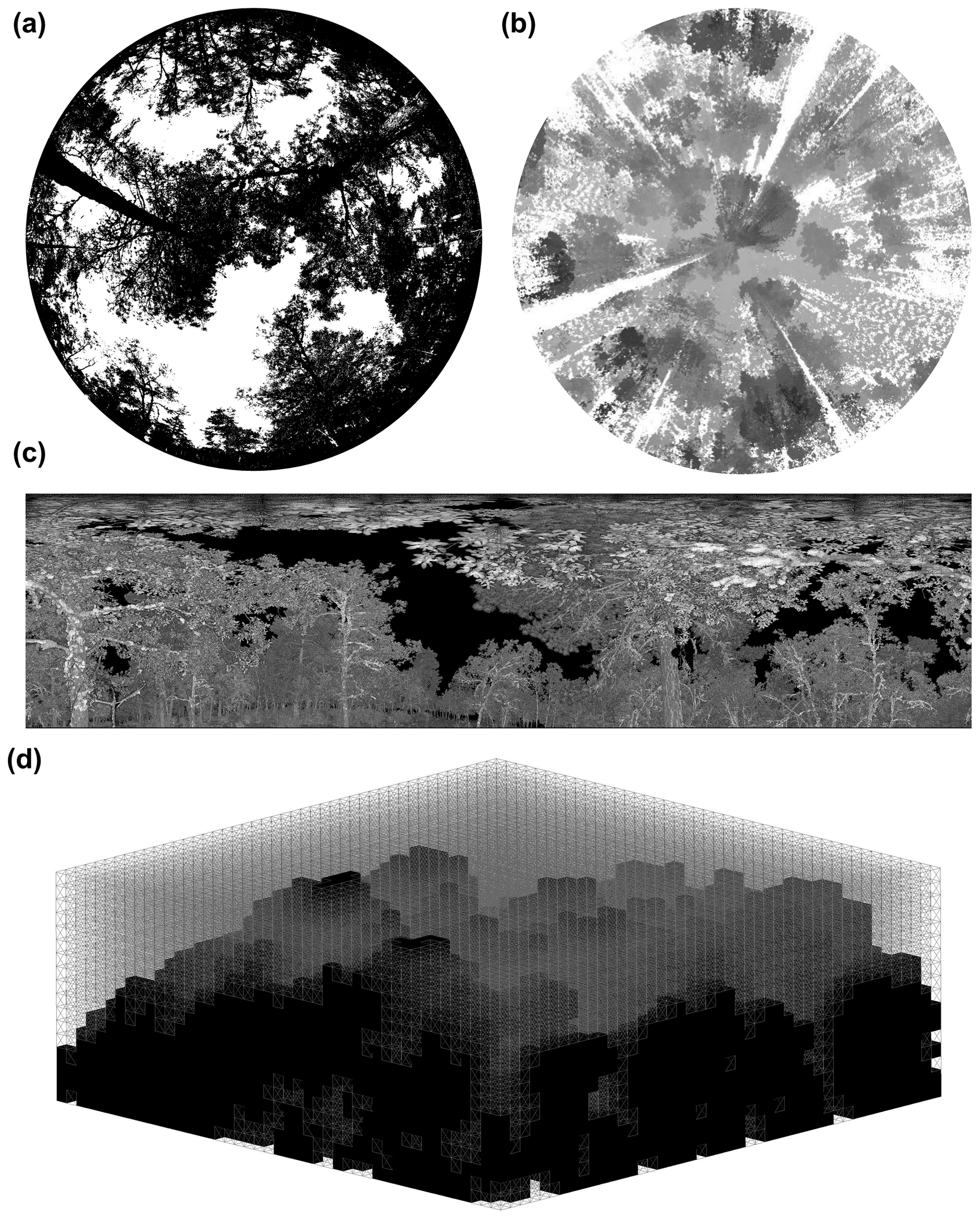
Figure 1 Visual representation of the four methods for PAI and WAI estimation used in this study: (a) a binarised digital hemispherical photograph (DHP), (b) TLS raw single-scan point cloud, for the lidar pulse method (Jupp et al., 2008). Image shows a top-down view of raw point cloud, and greyscale represents low (grey) and high (black) Z values, (c) TLS 2D intensity image for the 2D intensity image method (Zheng et al., 2013), (d) voxelised co-registered whole-plot point cloud for the voxel-based method (Hosoi and Omasa, 2006), showing a representative schematic of cube voxels with edge length of 1 m, voxelised using the R package VoxR (Lecigne et al., 2018). Solid black voxels are classified as containing vegetation (filled), and voxels outlined with grey lines are voxels classified as empty.

The ratio of wood to total plant area, α, is known to be dynamic, changing in response to abiotic and biotic conditions. For example, the Huber value (sapwood-to-leaf-area ratio, a related measure to α) may vary according to water availability (Carter and White, 2009). Leaf area may therefore be indicative of the drought tolerance level of a tree, with more drought-tolerant species displaying a lower leaf area, reducing the hydraulic conductance of the whole tree and therefore increasing its drought tolerance (Niinemets and Valladares, 2006). α has been hypothesised to increase with the size of a tree in response to the increased hydraulic demand associated with greater hydraulic resistance of tall trees (Magnani et al., 2000) and higher transpiration rates of larger LAI (Battaglia et al., 1998; Phillips et al., 2003). Stand density may also impact α (Long and Smith, 1988; Whitehead, 1978), as increased stand level water use scales linearly with LAI (Battaglia et al., 1998; Specht and Specht, 1989), reducing water availability to individual trees competing for the same resources (Jump et al., 2017). Large-scale quantification of α or Huber value, however, is difficult as studies usually rely on a small number of destructively sampled trees (e.g. Carter and White, 2009; Magnani et al., 2000), litterfall traps (e.g. Phillips et al., 2003) or masking hemispherical images (e.g. Sea et al., 2011; Woodgate et al., 2016). These approaches are only applicable on a small to medium scale, and in the case of image masking, cannot differentiate between individuals. Variation in α, for example by species and or stand structure, is therefore largely unknown.

1.1 TLS methods for calculating PAI, LAI and WAI

Terrestrial laser scanning (TLS) generates high-resolution 3D measurements of whole forests and individual trees (Burt et al., 2019; Disney, 2018), leading to the development of completely new monitoring approaches to understand the structure and function of ecosystems (Lines et al., 2022). Unlike traditional passive sensors, TLS can estimate PAI, WAI, and LAI for both whole plots and individual tree point clouds (Calders et al., 2018) and is unaffected by illumination conditions. This has led to the development of several methods for processing TLS data to extract the key metrics PAI, WAI and LAI (e.g. Hosoi and Omasa, 2006; Jupp et al., 2008; Zheng et al., 2013). However, intercomparison studies of algorithms and processing approaches to derive the same metrics from different TLS methods are lacking. TLS methods for extracting PAI, LAI and WAI can be broadly categorised into two types: (1) lidar return counting, using single-scan data (e.g. the lidar pulse method; Jupp et al., 2008, and 2D intensity image method; Zheng et al., 2013), and (2) point cloud voxelisation, usually using co-registered scans (e.g. the voxel-based method; Hosoi and Omasa, 2006).

The lidar pulse method (Jupp et al., 2008; Fig. 1b) estimates gap fraction (P_gap) using single-scan data, as a function of the total number of outgoing lidar pulses from the sensor and the number of pulses that are intercepted by the canopy. This method, which eliminates illumination impacts associated with the use of DHP (Calders et al., 2014), has been implemented in the Python module PyLidar (https://www.pylidar.org, last access: 11 July 2023) and the R package rTLS (Guzman, et al., 2021). Using the lidar pulse method, Calders et al. (2018) compared PAI estimates from two ground-based passive sensors (LiCOR LAI-2000 and DHP) with TLS data collected with a RIEGL VZ-400 TLS in a deciduous woodland and found the two passive sensors underestimated PAI values compared to TLS, with differences dependent on DHP processing and leaf on/off conditions.

The 2D intensity image method (Zheng et al., 2013; Fig. 1c) also uses raw single-scan TLS point clouds but, unlike the lidar pulse method, converts lidar returns into 2D panoramas where pixel values represent return intensity. PAI is estimated by classifying pixels as sky or vegetation, based on their intensity value, to estimate P_gap, and then applying Beer–Lambert's law. Like the lidar pulse method, this approach has been shown to generate higher PAI estimates than DHP (Calders et al., 2018; Woodgate et al., 2015; Grotti et al., 2020), with differences attributed to the greater pixel resolution and viewing distance of TLS resolving more small canopy details (Grotti et al., 2020).

The voxel-based method (Fig. 1d) estimates PAI by segmenting a point cloud into voxels and either simulating radiative transfer within each cube (Béland et al., 2014; Kamoske et al., 2019) or classifying voxels as either containing vegetation or not and dividing vegetation voxels by the total number of voxels (Hosoi and Omasa, 2006; Itakura and Hosoi, 2019; Li et al., 2017). Crucially, this method may be applied to multiple co-registered scan point clouds and so can be used to calculate PAI for both whole plots and individual, segmented TLS trees. However, PAI estimates derived using the voxel method are highly dependent on voxel size (Calders et al., 2020). Using a radiative transfer approach, Béland et al. (2014) demonstrated that voxel size is dependent on canopy clumping, radiative transfer model assumptions and occlusion effects, making a single, fixed choice of voxel size for all ecosystem types, scanners or datasets impossible. To test various approaches to selecting voxel size using a voxel classification approach, Li et al. (2016) matched voxel size to point cloud resolution, individual tree leaf size, and minimum beam distance and tested against destructive samples, finding that voxel size matched to point cloud resolution had the closest PAI values to destructive samples. The lidar pulse method and 2D intensity image method both use single-scan data. However, to generate robust estimates of canopy properties that avoid errors from occlusion effects, multiple co-registered scans taken from different locations are likely needed (Wilkes et al., 2017). Further, both these methods require raw unfiltered data to accurately measure the ratio of pulses emitted from the scanner and number of pulses that are intercepted by vegetation. This means “noisy” points caused by backscattered pulses (Wilkes et al., 2017) are included in analyses, potentially leading to higher PAI estimates. However, the lidar pulse and 2D intensity image methods may introduce fewer estimation errors compared to DHP, which is influenced by differences in sky illumination conditions and camera exposure (Weiss et al., 2004).

1.2 Scope and aims

The aims of this study are twofold: the first aim is to compare three TLS methods for estimating PAI with traditional DHP. The second aim of this study is to use TLS to understand drivers of individual tree α variation.

In this study we use a dataset of 528 co-located DHP and high-resolution TLS scans from 33 forest plots to compare DHP-derived PAI (PAI_DHP) with estimates from three methods to estimate PAI from TLS data (PAI_TLS): the lidar pulse method, the 2D intensity image method, and the voxel-based method (Fig. 1). We use a dataset collected from a network of pine–oak forest plots in Spain (Owen et al., 2021) and ask (1) are the three TLS methods able to reproduce PAI_DHP estimates at single-scan and whole-plot level? (2) Does α, calculated from the voxel-based method on individual tree point clouds, vary with species and tolerance to drought? And (3) does α scale with height and stand density?

2 Methods

2.1 Study site

We collected TLS and DHP data from 29 plots in Alto Tajo Natural Park (40^∘41^′N, 02^∘03^′ W; FunDIV – functional diversity plots; see Baeten et al., 2013, for a detailed description of the plots) and four plots in Cuéllar (41^∘23^′ N 4^∘21^′ W) in June–July 2018 (see Owen et al., 2021, for full details) (Fig. A1 in Appendix A). Plots contained two oak (Quercus) species and three pine (Pinus) species: semi-deciduous Q. faginea and evergreen Q. ilex and P. nigra, P. pinaster and P. sylvestris. P. sylvestris is the least drought-tolerant species, followed by P. nigra, Q. faginea and Q. ilex; shade tolerance follows the same ranking (Niinemets and Valladares, 2006; Owen et al., 2021). Although not quantitatively ranked, P. pinaster has been shown to be very drought tolerant, appearing in drier areas than the other species (Madrigal-González et al., 2017). The area is characterised by a Mediterranean climate (altitudinal range 840–1400 m a.s.l.) (Jucker et al., 2014; Madrigal-González et al., 2017). In addition to the five main canopy tree species, plots contained an understorey of Juniperus thurifera and Buxus sempervirens (Kuusk et al., 2018).

2.2 Field protocol

In each of the 33 plots of size 30 × 30 m, we collected TLS scans on a 10 m grid, making 16 scan locations following Wilkes et al. (2017) to minimise occlusion effects associated with insufficient scans. We used a Leica HDS6200 TLS set to super high resolution (3.1 × 3.1 mm resolution at 10 m with a beam divergence of ≤5 mm at 50 m; scan time 6 m 44 s; see Owen et al., 2021). At each of the 528 scan locations and following the protocol in Pfeifer et al. (2012), we captured co-located DHP images with three exposure settings (automatic and ± one stop exposure compensation), levelling a Canon EOS 6D full frame DSLR sensor with a Sigma EX DG F3.5 fisheye lens, mounted on a Vanguard Alta Pro 263AT tripod.

2.3 Calculation of single-scan and whole-plot PAI using DHP data

For each of the red–green–blue (RGB) DHP images we extracted the blue band for image thresholding, as this best represents sky–vegetation contrast (Pfeifer et al., 2012). For each plot, we picked the exposure setting that best represented sky–vegetation difference based on pixel brightness histograms of four sample locations indicative of the plot. We carried out automatic image thresholding using the Ridler and Calvard method (1978), to create a binary image of sky and vegetation, avoiding subjective user pixel classification (Jonckheere et al., 2005). We calculated PAI from the binary image, limiting the field of view to a 5^∘ band centred on the hinge angle of 57.5^∘ (55–60^∘). The hinge angle has a path length through the canopy twice the canopy height, so the band around it is an area of significant spatial averaging taken as representative of canopy structure of the area (Calders et al., 2018; Jupp et al., 2008). From the binarised hinge angle band we calculated P_gap as the number of sky pixels divided by the total number of pixels and PAI using an inverse Beer–Lambert law equation (Monsi and Saeki, 1953). We calculated whole-plot PAI as the arithmetic mean of the 16 plot scan location PAI estimates. As this value does not correct for canopy clumping, it is better described as effective PAI, rather than true PAI (Woodgate et al., 2015). However, as the TLS and DHP methods we apply here account for canopy clumping differently, we compared effective values and here on refer to effective PAI as PAI (Calders et al., 2018). DHP images used in this study are freely available (see Flynn et al., 2023).

2.4 Calculation of single-scan and whole-plot PAI from TLS data

To calculate PAI using the lidar pulse method (Jupp et al., 2008), we calculated P_gap for a single scan (Fig. 1b) by summing all returned laser pulses and dividing by the number of total outgoing pulses, following Lovell et al. (2011; see Eq. 7 in that study), and then estimated PAI following Jupp et al. (2008; see Eq. 18 in that study), setting the sensor range to 5^∘ around the hinge angle as before (55–60^∘). Single-scan PAI was taken as the cumulative sum of PAI values estimated by vertically dividing the hinge region into 0.25 m intervals (Calders et al., 2014). We implemented the lidar pulse method using the open-source R (R Core Team, 2022) package rTLS (Guzmán et al., 2021).

To calculate PAI using the 2D intensity image method (Zheng et al., 2013), we converted 3D TLS point cloud data from all 528 scan locations into polar coordinates, scaled intensity values to cover the full 0–255 range (Fig. 1c) and rasterised into a 2D intensity image using the open-source R package raster (Hijmans, 2022). We cut the 2D intensity image to a 5^∘ band around the hinge angle (55–60^∘) and classified sky and vegetation pixels in each image using the Ridler and Calvard method (1978). We calculated P_gap as the number of pixels classified as sky divided by the total number of pixels and derived PAI with an inverse Beer–Lambert law equation (Monsi and Saeki, 1953).

Following the same approach as applied to our DHP data, we calculated whole-plot PAI for the lidar pulse and 2D intensity image methods as the arithmetic mean of the 16 plot scan location PAI estimates.

To calculate PAI using the voxel-based method, we followed a voxel classification approach (Hosoi and Omasa, 2006), downsampling the point cloud to 0.05 m to aid computation time and matching the voxel size to the resolution of the point cloud, following Li et al. (2016), who showed that matching the voxel size to the point cloud point-to-point minimum distance (resolution) increases accuracy as small canopy gaps are not included in voxels classified as vegetation. We chose to use a voxel classification approach (rather than a radiative-transfer-based one) as this method is widely applicable to a range of TLS systems and levels of processing, as well as providing explicit guidance on voxel size selection, which is known to impact derived PAI estimates (Li et al., 2016). We re-combined individually segmented trees, filtered for noise using a height-dependent statistical filter (see Owen et al., 2021) back into whole-plot point clouds and voxelised them using the open-source R package VoxR (Lecigne et al., 2018), with a full grid covering the minimum to maximum xyz ranges of the plot. We classified any voxel containing >0 points as vegetation (“filled”) and empty voxels as gaps. We then split the voxelised point cloud vertically into slices one voxel high. Within each slice, the contact frequency is calculated as the fraction of filled to total number of voxels. We then multiplied the contact frequency by a correction factor for leaf inclination, set at 1.1 (Li et al., 2017), and whole-plot PAI was calculated as the sum of all slices' contact frequencies.

2.5 Calculation of individual tree PAI, WAI and α using the voxel-based method

As the only method using multiple co-registered scans, the voxel-based method is the only method compared in this study capable of deriving PAI, WAI and LAI of segmented individual tree point clouds. We estimated PAI and WAI for 2472 individual trees segmented from co-registered point clouds following a similar method to the whole-plot point cloud. We used individual tree point clouds downsampled to 0.05 m, to aid computation time, and segmented using the automated tree segmentation program treeseg (Burt et al., 2019), implemented in C$++$, by Owen et al. (2021) for that study. Individual segmented tree data used in this study are freely available (see Owen et al., 2022).

To estimate PAI, WAI and α for each tree, we used individual tree point clouds wood–leaf separated by Owen et al. (2021) using the open-source Python library TLSeparation (Vicari et al., 2019) and then used the separated wood point clouds to calculate WAI. TLSeparation assigns points as either leaf or wood, iteratively looking at a predetermined number of nearest neighbours (k-NN). The k-NN of each iteration is directly dependent on point cloud density, since high-density point clouds will require higher a k-NN (Vicari et al., 2019). The utility package in TLSeparation was used to automatically detect the optimum k-NN for each tree point cloud.

To voxelise individual tree complete (Fig. 2a) and wood only (Fig. 2b) point clouds, we used a modified approach based on Lecigne et al. (2018), voxelising within the projected crown area of the whole tree point cloud (Fig. 2c) to calculate PAI. In the same way as for PAI, we calculated WAI using the separated wood point cloud within the projected crown area of the whole tree (Fig. 2d; using the whole crown and not just the wood point cloud) and derived α for each tree as $\mathrm{WAI}/\mathrm{PAI}$, allowing a comparison with existing literature estimating α for a range of ecosystems (Sea et al., 2011; Woodgate et al., 2016).

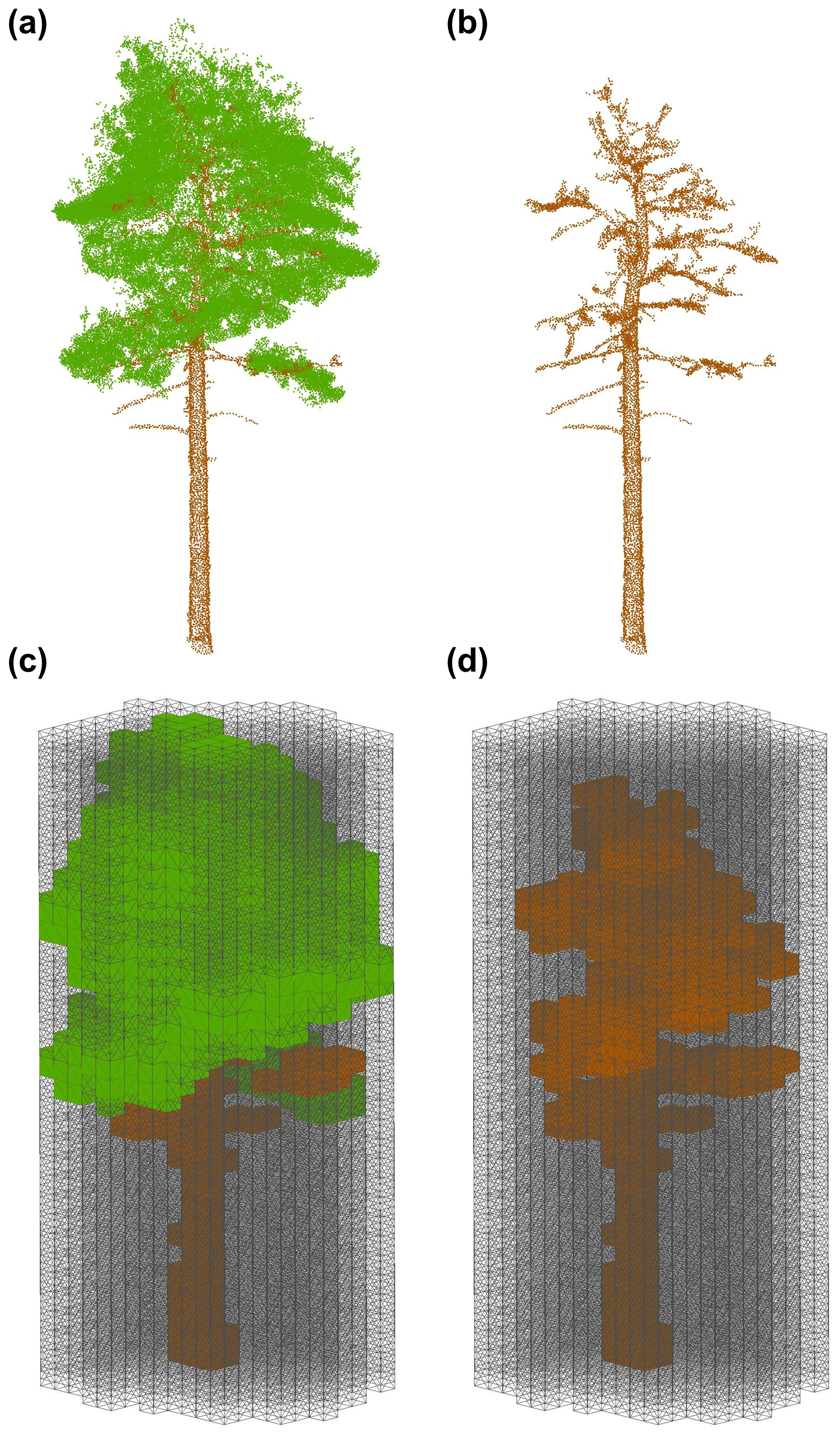
Figure 2 Visualisation of the workflow for applying the voxel-based method to estimate individual tree PAI, WAI and α. (a) Individual tree point cloud; (b) separated leaf off (wood) individual tree point cloud; (c) voxelised individual tree point cloud; (d) voxelised wood cloud. Coloured voxels (green represents leaf and brown represents wood) are filled voxels, and grey lines are empty voxels. Empty voxels occupy the space within the projected crown area of the tree. Image shows schematic of point cloud voxelised with cube voxels with edge length of 0.5 m. Panels (a) and (b) show wood and leaf separation of an example P. sylvestris, carried out using TLSeparation (Vicari et al., 2019). Point cloud voxelisation was carried out using modified functions from R package VoxR (Lecigne et al., 2018). Note that our method used voxel sizes at the resolution of the cloud (0.05 m), but here we present an image with larger voxels to ease visual interpretation.

2.6 Statistical analyses

We tested the relationships between PAI_TLS and PAI_DHP estimates using standardised major axis (SMA) using the open-source R (R Core Team, 2022) package smatr (Warton et al., 2012). SMA is an approach to estimating a line of best fit where we are not able to predict one variable from another (Warton et al., 2006); we chose SMA because we do not have a “true” validation dataset, so we avoid assuming either DHP or any of the TLS methods produce the most accurate results. For each TLS method, we assessed the relationship with DHP using the coefficient of determination and RMSE. We chose to compare PAI values rather than WAI or LAI as to do so would mean an additional correction for non-photosynthetic elements, which each method does in different ways, therefore introducing further sources of uncertainty and limiting our ability to fairly compare processing approaches. To further understand observed drivers of variance in PAI, we tested the relationship between PAI and whole-plot crown area index, CAI, a proxy measure of stand density and local competition (Caspersen et al., 2011; Coomes et al., 2012). We calculated CAI as the sum of TLS-derived projected crown area, divided by the plot area (Owen et al., 2021).

To test whether α differs by species, we used linear mixed models (LMMs) in the R package lme4 (Bates et al., 2015). We included an intercept only random plot effect to account for local effects on α:

$$\begin{array}{}\text{(1)}& {\mathit{\alpha }}_{i,sj}={\mathit{\phi }}_s+{\mathrm{Plot}}_j.\end{array}$$

Here, α_i is α of an individual of species s, in plot j, and φ_s is the parameter to be fit. To test the effect of stand structure and tree height on α, we fit relationships separately for each species, again including a random plot effect:

$$\begin{array}{}\text{(2)}& {\mathit{\alpha }}_{i,sj}={\mathit{\phi }}_s+b_s{H}_i+c_s{\mathrm{CAI}}_j+{\mathrm{Plot}}_{sj.}\end{array}$$

Here H_i is the height of the tree, and CAI_j is the crown area index for the plot, with other parameters as before.

For each species' model (Eq. 2), we calculated the intra-class correlation coefficient (ICC). The ICC, similar to coefficient of determination, quantifies the amount of variance explained by the random effect in a linear mixed model (Nakagawa et al., 2017).

3 Results

3.1 Comparison of plant area index estimated by DHP and single-scan TLS

Of the two single-scan TLS methods tested (lidar pulse method and 2D intensity image method), we found that the relationship between PAI estimated using the lidar pulse method and PAI_DHP had a higher R² than the 2D intensity image method (SMA; lidar pulse method R²=0.50, slope = 0.73, p<0.001, RMSE = 0.14 and 2D intensity image method R²=0.22, slope = 0.38, p<0.001, RMSE = 0.39, respectively, Fig. 3a). At larger PAI values, both TLS methods underestimated PAI relative to DHP (Fig. 3b). We found statistically significant negative correlations between residuals and DHP for both methods (SMA; 2D intensity image method residuals R²=0.85, slope = −0.88, p<0.01; lidar pulse method residuals R²=0.47, slope = −0.70, p<0.01; Fig. 3b). The 2D intensity image method showed larger underestimation at higher PAI_DHP values, suggesting this method may saturate sooner for higher PAI values than either DHP or the lidar pulse method (Fig. 3b).

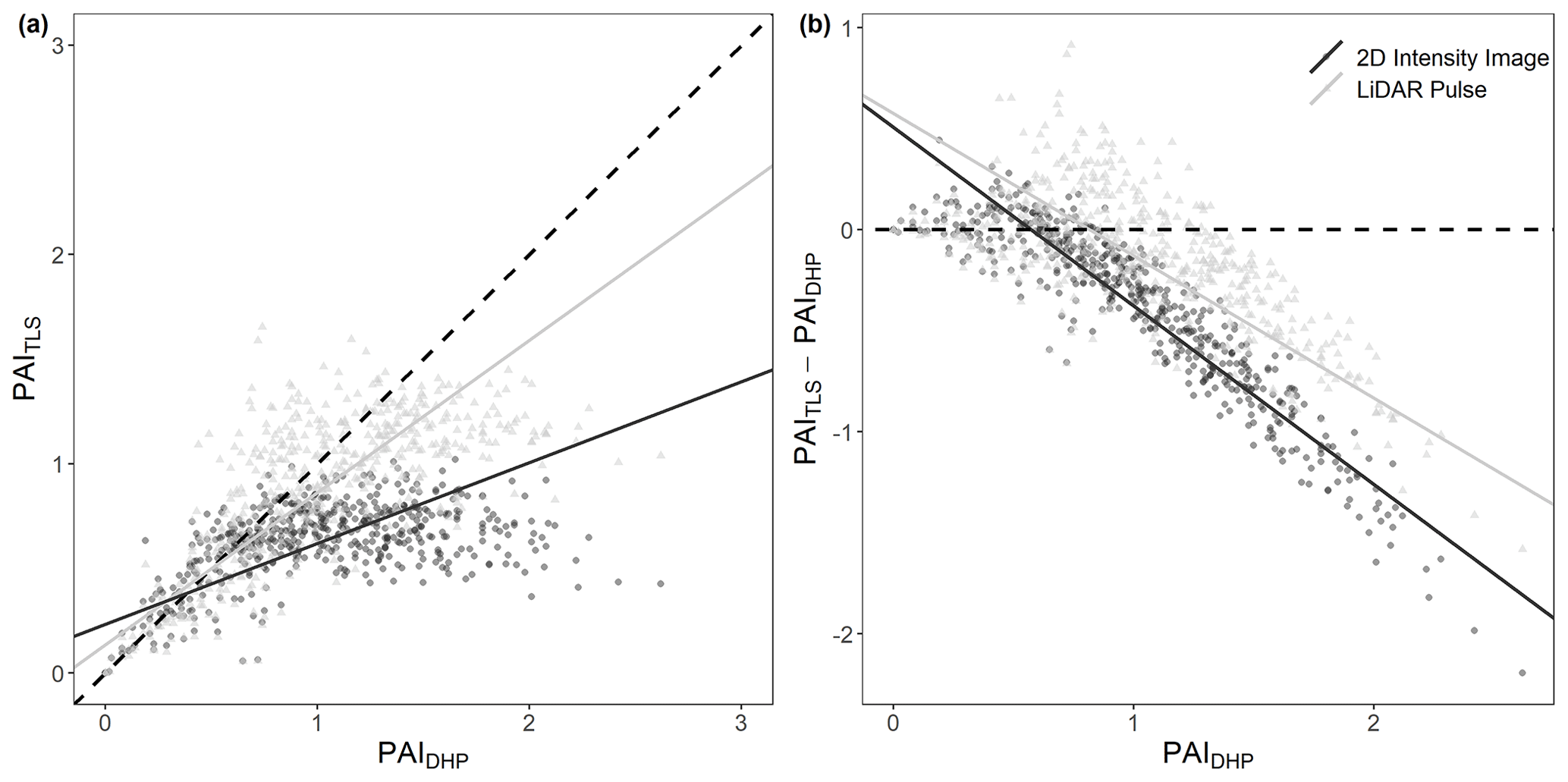
Figure 3 Comparison of single-scan PAI_TLS and PAI_DHP estimates, for all 528 scan locations (16 per plot). (a) The correlation between DHP-derived PAI with PAI derived using the 2D intensity image method R²=0.22, slope = 0.38, p<0.001, RMSE = 0.39 (circles), and lidar pulse method R²=0.50, slope = 0.73, p<0.001, RMSE = 0.14 (triangles). Dashed line in (a) represents 1 : 1 relationship. (b) The difference between PAI_TLS and PAI_DHP estimates for the 2D intensity image method and lidar pulse method. Dashed line in (b) represents 0. Solid lines show statistically significant relationships fitted using SMA (p<0.01).

3.2 Comparison of whole-plot plant area index estimated using TLS and DHP and the effect of plot structure on PAI

We found statistically significant correlations between whole-plot PAI_TLS values and PAI_DHP for all three TLS methods (Fig. 4). As for single scans, the lidar pulse method showed the closest agreement to PAI_DHP, here compared to both the voxel-based and 2D intensity image methods (SMA; lidar pulse method R²=0.66, slope = 0.82, p<0.01, RMSE = 0.14; voxel-based method R²=0.39, slope = 2.76, p<0.01, RMSE = 0.88; 2D intensity image method R²=0.35, slope = 0.36, p<0.01, RMSE = 0.39, respectively; Fig. 4a). The 2D intensity image method and lidar pulse method consistently underestimated PAI compared to DHP, whilst the voxel-based method underestimated in plots with lower PAI_DHP and overestimated in plots with higher PAI_DHP. The voxel-based method's high PAI values compared to other methods are likely due to its use of multiple co-registered scans reducing occlusion effects prevalent in single-scan data.

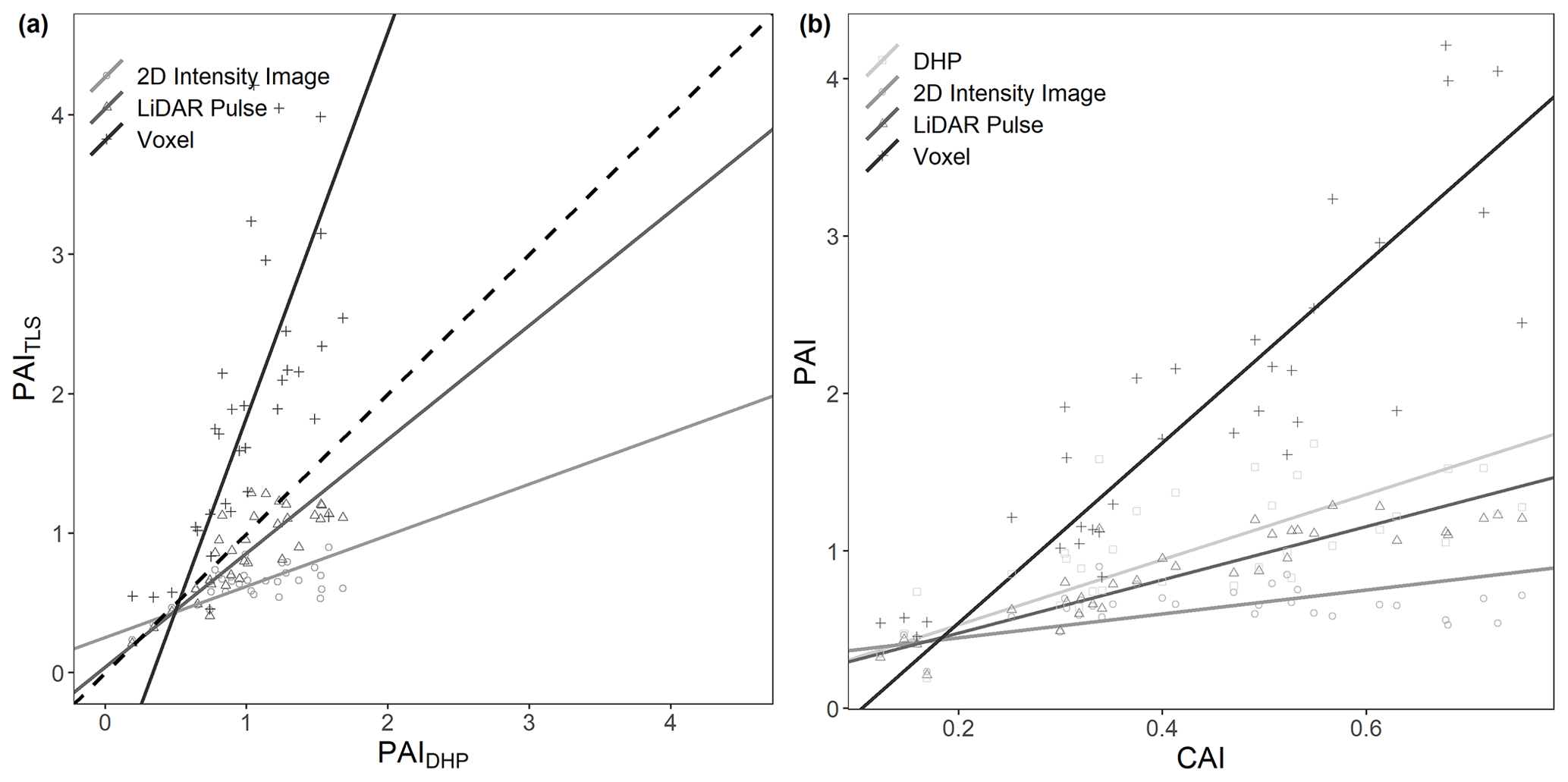
Figure 4 Comparison of plot level PAI_TLS vs. PAI_DHP and CAI vs. PAI estimates for all 33 plots. (a) The correlation between DHP-derived PAI and PAI derived using 2D intensity image R²=0.35, slope = 0.36, p<0.01, RMSE = 0.39 (circle), lidar pulse R²=0.66, slope = 0.82, p<0.01, RMSE = 0.14 (triangle) and voxel-based R²=0.39, slope = 2.76, p<0.01, RMSE = 0.88 (cross) methods. (b) The correlation between TLS-derived CAI and PAI derived using DHP R²=0.46, slope = 2.07, p<0.01 (square), 2D intensity image R²=0.15, slope = 0.76, p<0.05 (circle) lidar pulse R²=0.79, slope = 1.69, p<0.01 (triangle) and voxel-based R²=0.76, slope = 5.72, p<0.01 (cross) methods. Lines show statistically significant relationships fitted using SMA (p<0.01). Dashed line in (a) represents 1 : 1 relationship.

To assess the effect of plot structure on variation in TLS-derived PAI, we compared PAI_TLS estimates with TLS-derived CAI (Fig. 4b). We found a significant positive relationship between CAI and PAI estimated using each of the lidar pulse method, the voxel-based method and DHP (SMA; lidar pulse method R²=0.79, slope = 1.69, p<0.01; voxel-based method R²=0.76, slope = 5.72, p<0.01; 2D intensity image method R²=0.15, slope = 0.76, p<0.05; DHP R²=0.46, slope = 2.07, p<0.01, respectively; Fig. 4b), where the 2D intensity image method shows signs of saturation at medium CAI values (Fig. 4b).

3.3 Influence of species, tree height and CAI on α

To understand drivers of variance in α, we used individual tree PAI and WAI, calculated using the voxel-based method to test the relationship between species and α and the relationship between height/CAI and α. We found that more drought-tolerant species generally had higher α values than less drought-tolerant species (Table B1 in Appendix B; Fig. 5); however, confidence intervals were wide and overlapping, suggesting that species is not a strong predictor of variation in α. We found a statistically significant negative effect of height (p<0.001; Table B2; Fig. 6a) and positive effect of CAI (p < 0.01–0.05; Table B2; Fig. 6b) on α for all species apart from P. sylvestris. α decreased more rapidly with height and increased less rapidly with CAI for oaks than pines. Statistically significant ICC values were higher for P. nigra (ICC = 0.211; Table B2) than P. pinaster, Q. faginea and Q. ilex (ICC = 0.036; 0.060; 0.070, respectively), showing that more α variation is explained by the random plot effect in P. nigra than the other species. P. pinaster has a wider confidence interval (Fig. 5), possibly explained by its lower sample size. To understand drivers of variance in WAI we carried out additional analysis to test the relationship between WAI and species, height, CAI and PAI and presented these results in Appendix C (Fig. C3; Tables C3, C4).

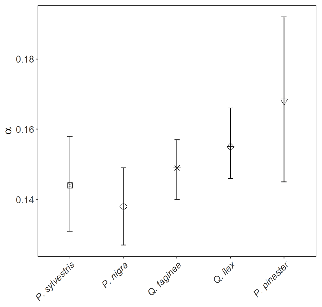
Figure 5 Linear-mixed-model-derived α values (φ, Eq. 1) for all 2472 individual trees of species P. sylvestris, P. nigra, Q. faginea, Q. ilex and P. pinaster. Error bars represent 95 % confidence intervals. Species are listed left to right from low–high drought tolerance, with the exception of P. pinaster, for which drought tolerance index has not been calculated in the literature. Drought tolerance rankings are taken from Niinemets and Valladares (2006).

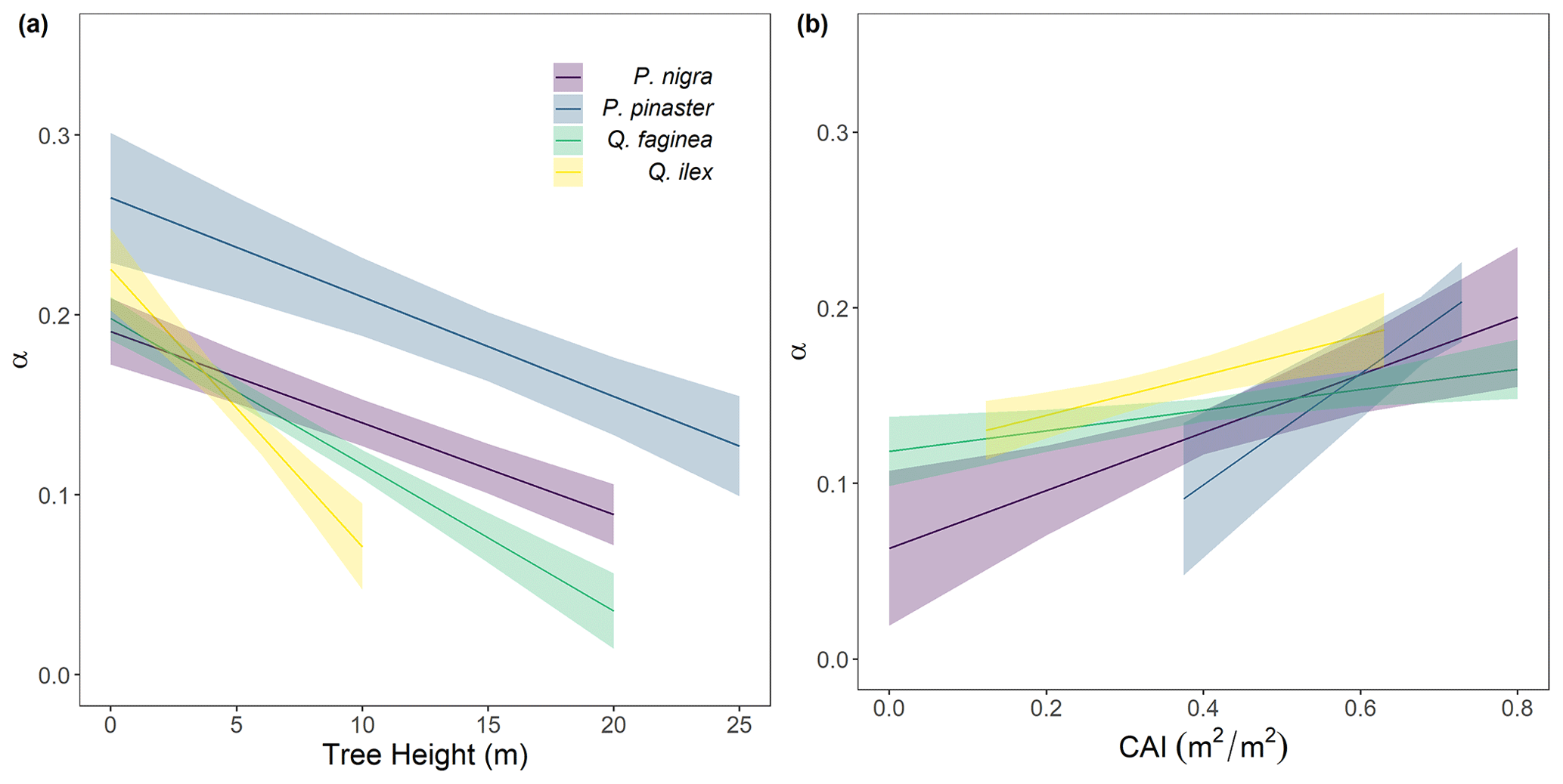
Figure 6 Variation in α for each species: Pinus nigra, P. pinaster, Q. faginea and Q. ilex with (a) height and (b) plot CAI. Lines represent statistically significant linear mixed models (Eq. 2; significance levels from p<0.001 to p<0.05). Ribbons represent 95 % confidence intervals. The model for P. sylvestris was not statistically significant.

4 Discussion

4.1 Comparison of approaches to deriving PAI from remote sensed data

We found substantial differences in PAI values estimated from TLS and DHP and from different TLS processing methods (Figs. 3 and 4). Further, differences between TLS methods varied across plot structure, with the greatest differences between methods in plots with high CAI and therefore high canopy density. Although previous studies have presented TLS as an improvement over DHP due to its independence of illumination and sky conditions during the data acquisition phase and ability to resolve fine-scale canopy elements and gaps (Calders et al., 2018; Grotti et al., 2020; Zhu et al., 2018), we have shown that there is large variability between TLS processing methods in Mediterranean forests. Rigorous intercomparison of approaches, ideally using standard benchmarking TLS datasets, and destructive sampling, would improve trust and reliability of TLS algorithms.

We found the lidar pulse method (Jupp et al., 2008) to have the best agreement with DHP for both whole-plot and single-scan PAI estimates. In contrast to previous studies comparing PAI_TLS with PAI_DHP (Calders et al., 2018; Grotti et al., 2020; Woodgate et al., 2015), we found that the lidar pulse and 2D intensity image methods underestimated PAI compared to DHP, except at very low PAI values (PAI_TLS < 0.5). Quantification of PAI from DHP may introduce additional sources of error; for example, its relatively lower resolution compared to TLS could lead to mixed pixels that have a greater chance of misclassification of sky as vegetation (Jonckheere et al., 2004). This effect could be enhanced in a Mediterranean forest as trees in drier climates tend to have smaller leaves (Peppe et al., 2011), leading to more small canopy gaps that TLS may resolve where DHP cannot. Further, although we took steps to reduce the error introduced at DHP data acquisition and processing steps, including using automatic thresholding and collecting images with multiple exposures, DHP processing requires both model and user assumptions that can impact results. For example, PAI_DHP estimates are highly sensitive to camera exposure; increasing one stop of exposure can result in 3 %–28 % difference in PAI, and use of automatic exposure can result in up to 70 % error (Zhang et al., 2005).

We found the voxel-based method overestimated PAI values compared to the other methods at the whole-plot level. This is likely due to the method's use of co-registered scans, rather than averaged single-scan PAI values, since co-registered scans will reduce occlusion effects prevalent in single-scan data that could to lead to an underestimation of PAI (Wilkes et al., 2017). The voxel-based method is, however, sensitive to voxel size (Li et al., 2016), and larger voxels lead to larger PAI estimates as they are unable to capture all of the intricate details of canopy structure; we chose a voxel size of 0.05 m to match the minimum distance between points in our downsampled dataset. However, the voxel-based method is a memory-intensive approach to calculating PAI, and smaller voxels have higher memory requirements. We picked this data resolution, and therefore voxel size, to balance the need to capture fine-scale canopy details against memory requirements for running the method on many large plot point clouds. Voxel size could have been chosen based on estimates' match to DHP, but this would assume (1) that DHP estimates are most accurate and (2) that DHP data are always available, limiting the wider applicability of our findings. Understanding which method is over- or underestimating would require a destructively sampled dataset for validation, which was not possible for this study (or most ecosystems). However, other studies using voxel approaches have found that although these produce high LAI values for individual trees, these are underestimates compared with destructive samples (Li et al., 2016). Regardless, PAI and LAI estimates using a voxel-based approach are highly dependent on voxel size (Li et al., 2016), and future work should test the influence of voxel size on PAI estimates, using destructive samples in a range of environments.

The relationship between the lidar pulse method and TLS-derived CAI had the highest R², demonstrating that the method is well suited to measuring PAI across the range of plot CAI values used in this study. Although the 2D intensity image method can tackle the significant challenges presented by edge effects and partial beam interceptions, particularly present in phase-shift systems (Grotti et al., 2020), our results suggest this method has a lower performance ability, with saturation occurring sooner than all other methods in dense forests (Figs. 3 and 4). The 2D intensity image method uses the same raw single-scan data as the lidar pulse method, so the better performance from the latter is likely due to the method's use of vertically resolved gap fraction; both the lidar pulse method and voxel-based method account for the vertical structure of the canopy by summing vertical slices through the canopy.

4.2 α variation between species and plot

We used the voxel-based method to investigate individual tree α variation between species and across structure, as this was the only approach we compared that could be applied to single tree point clouds which are leaf–wood separated. We found α values obtained were within the range of values obtained from destructive approaches (0.1–0.6, Gower et al., 1997). The drought- and shade-intolerant P. nigra showed stronger variability in α across plots (higher ICC value, Table B2) than other species, suggesting its wood–leaf ratio may be more sensitive to site factors. However, as the plots measured in this study vary in both abiotic conditions (altitude, aspect, slope, wetness) as well as species composition, stem density and canopy cover, there may be other drivers of variation in α values.

We found some evidence that species with higher drought tolerance had higher α values (Fig. 5; Table B1); however, confidence intervals were wide, suggesting a weak relationship. There is evidence that trees that tolerate water-limited environments have a lower leaf area (Battaglia et al., 1998; Mencuccini and Grace, 1995), so higher α values may reflect maintenance of homeostasis of leaf water use through adjustment of wood-to-leaf-area ratio (Carter and White, 2009; Gazal et al., 2006). The potential for a tree to lose water is mostly regulated through leaf traits including stomatal conductance and leaf area, and both stand (Battaglia et al., 1998; Specht and Specht, 1989) and individual tree (Mencuccini, 2003) water use have been found to scale linearly with LAI, with drought often mitigated through leaf shedding (López et al., 2021).

4.3 Tree stature and stand density drive α variation

Although species had a weak relationship with α, tree height and plot CAI had a statistically significant relationship with α (p<0.001–p<0.05) for all species, showing the importance of local stand structure on leaf and woody allocation. We found that α scaled negatively with height for all species apart from P. sylvestris, suggesting that in this environment, taller trees generally have a lower proportion of wood to plant area index than shorter ones. P. sylvestris, which is at the edge of its geographical range and physiological limits (Castro-Díez et al., 1997; Owen et al., 2021), showed no significant relationship between height and α. We found that α scaled positively with plot level CAI for all species apart from P. sylvestris; that is, trees growing in denser plots have a higher α. This supports theory that trees growing in dense forests are competing for resources, reducing individual tree leaf area (Jump et al., 2017). The negative relationships between height and α and positive relationships between CAI and α relationships in our model suggest that trees may initially invest in vertical growth to reach the canopy level and once there invest in lateral growth, with more leaf area, to increase light capture. This supports theory that trees grow to outcompete neighbouring individuals for light capture (Purves and Pacala, 2008) and evidence that both lateral growth and LAI are reduced beneath closed canopies (Beaudet and Messier, 1998; Canham, 1988).

Wood may be harder to accurately classify than leaves in TLS data (Vicari et al., 2019), resulting in a higher occurrence of false positives in wood clouds, potentially leading to an overestimation in WAI, and therefore underestimation of α, especially in trees with small leaves which are prevalent in dry, Mediterranean environments (Peppe et al., 2011). The problem of misclassification will increase in taller trees due to TLS beam divergence, occlusion and larger beam footprint at further distances (Vicari et al., 2019), suggesting that WAI overestimation could be more pronounced in tall trees. Although our dense scanning strategy (Owen et al., 2021) was designed to mitigate some of these effects, these effects mean our findings may underestimate the slope of the negative relationship between α and tree height. Conversely, the increasing leaf-to-wood ratio could potentially be explained by a greater number of empty voxels caused by occlusion in large trees. However, we took significant steps to reduce occlusion, employing a 10 m scanning strategy that was developed in a dense tropical forest (Wilkes et al., 2017).

4.4 Correcting for non-photosynthetic elements in LAI estimates using TLS

The value of TLS data to estimate individual tree PAI, WAI and subsequently α demonstrates their potential to correct for non-photosynthetic components in ground-based remote sensing measurements of LAI. Properly correcting for WAI in LAI estimates is of global importance as small errors in ground-based measurements propagate through to large-scale satellite observations generating large errors in global vegetation models (Calders et al., 2018). The work presented here provides a foundation for future work combining multi-source and multi-scale remote sensing datasets to correct large-scale LAI products. Our results echo others in finding that the prevalence of woody material in the tree canopy, and therefore α is dynamic and varies by species as well as senescence, crown health and, in the case of deciduous forests, leaf phenology (Gower et al., 1999). The use of single α value in a plot or region (Olivas et al., 2013; Woodgate et al., 2016), invariant of species, size and forest structure, to convert PAI to LAI is therefore problematic (Niu et al., 2021). Our study demonstrates the importance of taking species mix and structural variation into account when correcting for non-photosynthetic material in ground-based LAI estimates.

5 Conclusions

We tested three methods for estimating PAI using terrestrial laser scanning data and compared these against traditional DHP measurements. We found large variation between PAI values estimated from each TLS method and DHP, demonstrating that care should be taken when deriving PAI from ground-based remote sensing methods. Although the lidar pulse method was found to have the best agreement with both single-scan and whole-plot PAI values measured by DHP, the voxel-based method allowed separate analysis of the key metric used to correct for the effect of WAI in LAI measurements, α, in individual trees. We recommend the lidar pulse method as a fast and effective method for PAI estimation independent of illumination conditions. Whilst the voxel-based method may be used to analyse individual tree α and determine ecological drivers of variation, work remains to determine the validity of these approaches, in particular correct voxel size choice. We found that α varies by species, height and stand density, showing the importance of accurately correcting for WAI on the individual tree level and the utility of TLS to do so.

The variation in our results for the different methods used to derive PAI from TLS data shows that there is some way to go before TLS-derived vegetation indices can be interpreted as robust and reliable. Validation using destructive samples and further intercomparison studies of methods are needed to demonstrate the advantages of TLS, and use of benchmarking datasets should be standard. DHP is a faster, cheaper and more widely accessible method for PAI estimation, and while TLS promises to alleviate potential bias in DHP estimates, results are highly method dependent. Our results demonstrate the challenges that stand in the way of large-scale adoption of TLS for vegetation index monitoring.

Appendix A

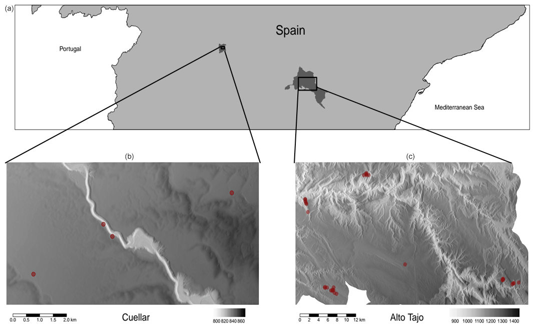
Figure A1 Map of plot locations within two field sites in central Spain (Cuéllar, b and Alto Tajo, c). Red points show plot locations on high-resolution digital terrain models enhanced with hillshading shown in greyscale (taken from the Supplement of Owen et al., 2021).

Appendix B

Table B1 Species–α linear mixed model (Eq. 1) showing relationship between tree species and α for all 2472 individual trees. Species are listed from low–high drought tolerance, with the exception of P. pinaster, for which drought tolerance index has not been calculated in the literature.

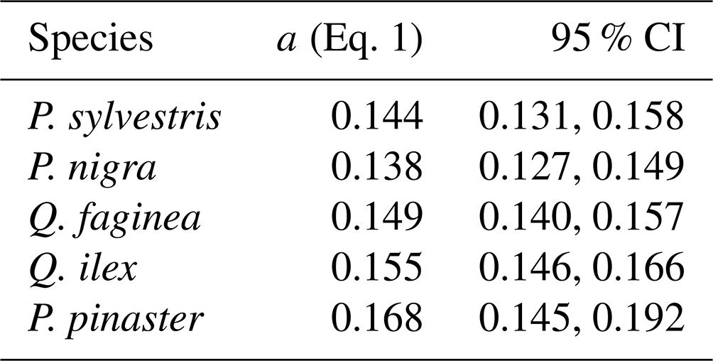
95 % CI denotes the 95 % confidence intervals.

Table B2 Height–α linear mixed models for each species (Eq. 2) showing relationship between tree height and plot CAI and α for all 2472 individual trees. Species are listed from low–high estimated α.

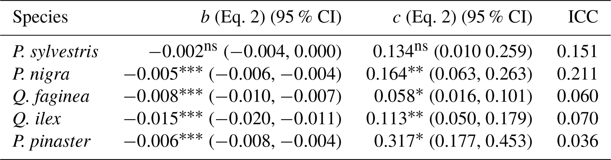
Significance codes: p<0.001 ${}^{***}$; p<0.01 ${}^{**}$; p<0.05 ^*; not significant ^ns; 95 % CI denotes the 95 % confidence intervals, and ICC is the intra-class correlation coefficient.

Appendix C

$$\begin{array}{}\text{(C1)}& {\displaystyle }\mathrm{WAI}=m_{\mathrm{species}}\text{(C2)}& {\displaystyle }\mathrm{WAI}=m\mathrm{height}+b\text{(C3)}& {\displaystyle }\mathrm{WAI}=m\mathrm{CAI}+b\text{(C4)}& {\displaystyle }\mathrm{WAI}=m\mathrm{PAI}+b,\end{array}$$

where WAI is the wood area index; species, height, CAI and PAI are the tree species, tree height, crown area index of the plot in which the tree is growing and tree plant area index respectively, and m and b are parameters to be fit.

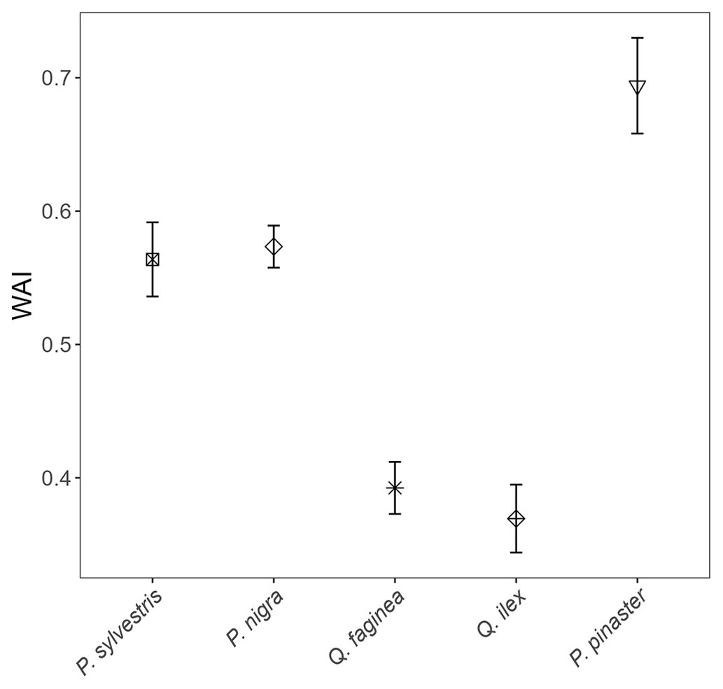
Figure C1 Linear-model-derived WAI values (m, Eq. C1) for all 2472 individual trees of species P. sylvestris, P. nigra, Q. faginea, Q. ilex and P. pinaster. Error bars represent 95 % confidence intervals. Species are listed from low–high drought tolerance, with the exception of P. pinaster, for which drought tolerance index has not been calculated in the literature. Between-species differences in WAI are likely primarily driven by differences in average tree height.

Table C1 Linear model (Eq. C1) showing relationship between tree species and WAI for all 2471 individual trees.

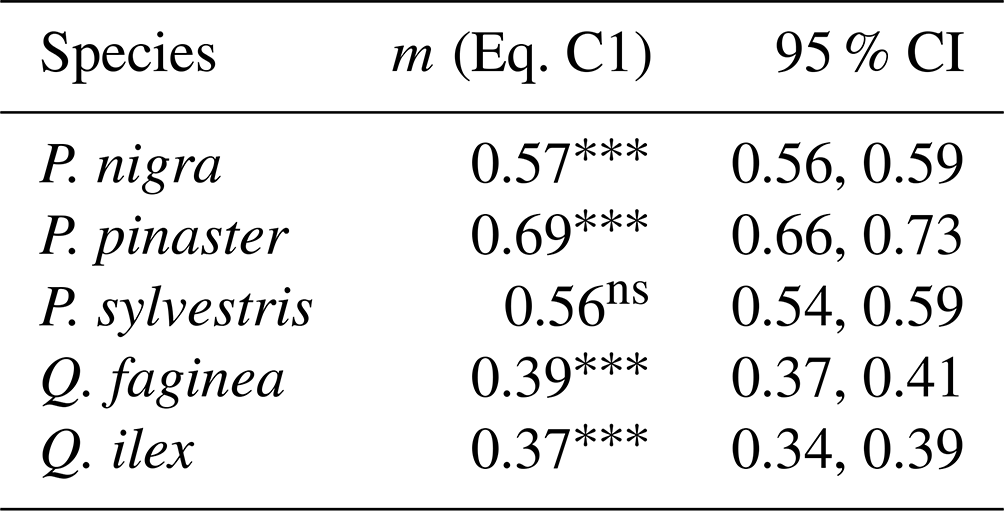
Significance codes: p<0.001 ${}^{***}$; p<0.01 ${}^{**}$; p<0.05 ^*; not significant ^ns; 95 % CI denotes the 95 % confidence intervals.

Table C2 Linear models (Eqs. C2, C3, C4) predicting WAI as a function of tree height, CAI (density) and PAI.

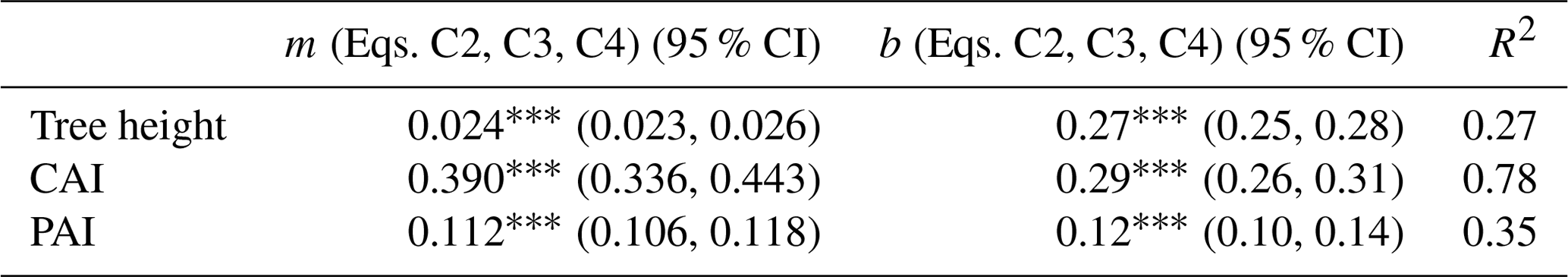
Significance codes: p<0.001 ${}^{***}$; p<0.01 ${}^{**}$; p<0.05 ^*; not significant ^ns; 95 % CI denotes the 95 % confidence intervals.