Simulated methane emissions from Arctic ponds are highly sensitive to warming

The Arctic is warming at an above-average rate, and small, shallow waterbodies such as ponds are vulnerable to this warming due to their low thermal inertia compared to larger lakes. While ponds are a relevant landscape-scale source of methane under the current climate, the response of pond methane emissions to warming is uncertain. We employ a new, process-based model for methane emissions from ponds (MeEP) to investigate the methane emission response of polygonal-tundra ponds in northeastern Siberia to warming.

MeEP is the first dedicated model of pond methane emissions which differentiates between the three main pond types of the polygonal-tundra, ice-wedge, polygonal-center, and merged polygonal ponds and resolves the three main pathways of methane emissions – diffusion, ebullition, and plant-mediated transport. We perform idealized warming experiments, with increases in the mean annual temperature of 2.5, 5, and 7.5 ^∘C on top of a historical simulation. The simulations reveal an approximately linear increase in emissions from ponds of 1.33 g CH₄ yr^−1 ∘C⁻¹ m⁻² in this temperature range. Under annual temperatures 5 ^∘C above present temperatures, pond methane emissions are more than 3 times higher than now. Most of this emission increase is due to the additional substrate provided by the increased net productivity of the vascular plants. Furthermore, plant-mediated transport is the dominating pathway of methane emissions in all simulations. We conclude that vascular plants as a substrate source and efficient methane pathway should be included in future pan-Arctic assessments of pond methane emissions.

1 Introduction

Waterbodies cover large parts of the Arctic landmasses (Muster et al., 2017), and ponds (surface area $<\mathrm{8}\times {\mathrm{10}}^{\mathrm{4}}$ m²; Ramsar Convention Secretariat, 2016) are the most numerous among them (Downing et al., 2006; Polishchuk et al., 2018; Muster et al., 2019). These ponds are a relevant component within the Arctic carbon cycle (Abnizova et al., 2012), as they emit carbon dioxide and, notably, methane (Wik et al., 2016; Holgerson and Raymond, 2016; Beckebanze et al., 2022). In a pan-Arctic synthesis study, Kuhn et al. (2021) show that more than 30 % of the total waterbody methane emissions come from small waterbodies (<0.1 km²), even though they only cover 10 % of the water-body area. This paper explores how pond methane emissions might change under higher temperatures.

The Arctic is warming rapidly (Chapman and Walsh, 1993; Bekryaev et al., 2010; Rantanen et al., 2022), which induces a multitude of changes to the permafrost landscape and to the embedded ponds specifically. Ponds are vulnerable to climate change due to their small size and low thermal inertia compared to lakes. During longer ice-free seasons, more water is lost to evaporation and subsurface runoff (Anderson et al., 2013; Riordan et al., 2006). So far, Arctic ponds have been sustained by the frozen ground, which has a low hydraulic permeability. Loss of permafrost, in turn, promotes drainage (Jepsen et al., 2013). While ponds are already disappearing in some regions, such as in discontinuous permafrost landscapes in Alaska (Riordan et al., 2006; Andresen and Lougheed, 2015), other regions might become richer in ponds with warming (Christensen et al., 2004; Bring et al., 2016).

The ice-wedge polygonal tundra is a landscape type that typically features a high pond density. Polygonal tundra covers roughly 3 % of the landmasses in the Arctic (Minke et al., 2007). It forms because temperatures drop far below freezing in winter; consequently, the soil contracts, and tension cracks open up. These cracks fill with meltwater in the spring before the soil can expand again. If this process repeatedly occurs, ice wedges eventually form just below the active layer (Jorgenson et al., 2015). The cracks often occur in shapes that resemble polygons (Cresto Aleina et al., 2013), and the formation of the ice wedges leads to movement of material from the center of the polygon to the edges, resulting in dry rims on top of the ice wedges and moist centers in the middle of the polygons (Minayeva et al., 2016). Melting of ice wedges is likely accompanied by increased formation of ponds (Jorgenson et al., 2006; Liljedahl et al., 2016). If the ice wedge itself degrades, a water-filled trough forms on top. These ponds are often elongated, and the remainder of the ice wedge constitutes part of the pond bottom, leading to cold bottom temperatures. These ponds are labeled ice-wedge ponds. If the middle part of a polygon subsides in between the ice wedges, then a nearly circular pond develops with a flat bottom. We call these ponds polygonal-center ponds. Finally, sometimes several polygons subside, leading to comparably large submerged areas, though the polygonal structure is often visible at the pond edge and bottom. We label these ponds merged polygonal ponds. These three pond types exhibit different methane dynamics (Rehder et al., 2021).

Most Arctic ponds emit predominantly contemporary, recently fixed carbon (Negandhi et al., 2013; Bouchard et al., 2015; Dean et al., 2020). However, newly formed ice-wedge ponds might emit older carbon than the average Arctic pond. When the permafrost adjacent to the thawing ice wedge degrades, old carbon can leech from the thawed sediments into the pond, additionally fueling methanogenesis (Langer et al., 2015; Prėskienis et al., 2021) and exerting a positive climatic feedback.

Furthermore, the composition of the ponds' methanogenic communities might change in response to the warming Arctic. Zhu et al. (2020) predicted that this will lead to an additional, strong increase in pond methane emissions. Besides temperature, methanogenesis in waterbodies depends on substrate availability. In permafrost soils, methanogens predominately use hydrogen and carbon dioxide or acetate, and increasing quantities of these substrates in the soil increase the rate of methanogenesis (de Jong et al., 2018). Vascular plants are one source of substrate (Joabsson and Christensen, 2001; Rehder et al., 2021), and vegetation and its composition in the Arctic are already changing (Villarreal et al., 2012; Bhatt et al., 2013). As a consequence methane emissions from Arctic ponds are expected to undergo substantial changes.

We aim to explore how pond methane emissions might change in a warmer Arctic and analyze as many of these interlinked effects on methane cycling in a single study as possible by employing the model MeEP (Methane Emissions from Ponds). MeEP is the first model specifically developed to represent the distinct ponds of the polygonal tundra on the landscape scale (here about 5 km²) and, notably, includes plant-mediated transport in addition to diffusion and ebullition. While diffusion and ebullition are usually accounted for, the impact of plant-mediated transport on landscape-scale fluxes from ponds is usually not considered, but we expect it to be as important as the other two fluxes.

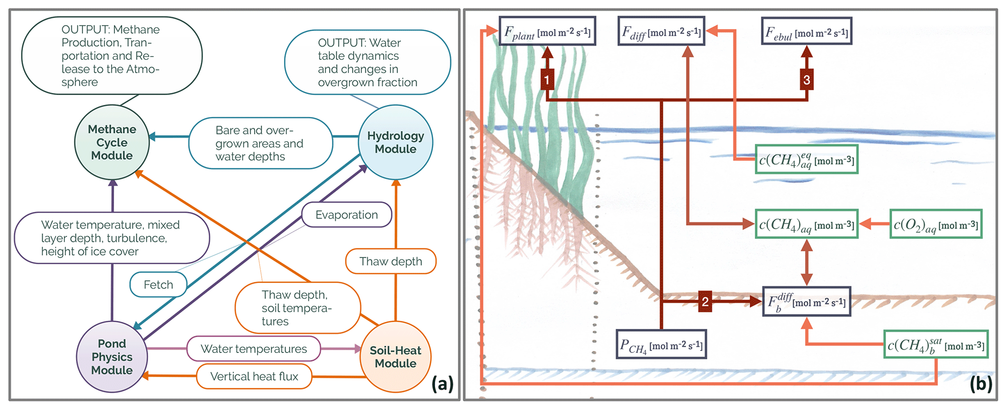
Figure 1 (a) Overview of the modules constituting MeEP. The variables which are used to couple the modules label the arrows in between the modules. The output of the methane and hydrological modules which we use in this work is listed as well. (b) Overview of the methane module with the main variables. F_plant denotes the plant-mediated transport, F_diff stands for the diffusive flux from water to the atmosphere, and F_ebul stands for ebullition. $P_{{\mathrm{CH}}_{\mathrm{4}}}$ is the rate of methanogenesis, and $F_{\mathrm{b}}^{\text{diff}}$ is the diffusion from the sediment to the atmosphere. Finally, c indicates concentration, the subscript aq labels dissolved gases, b is the sediment, and the superscript eq is concentration in equilibrium with the atmosphere.

2 Materials and methods

2.1 Short description and setup of MeEP

MeEP consists of four coupled modules: a pond-physics module; a soil-heat module; a hydrological module; and, the main focus of this work, a methane module. All modules operate at the same temporal resolution with time steps of 1 h (Fig. 1a). The pond physics, hydrological, and methane modules are one-dimensional, while the soil-heat module laterally couples pond sediments with the surrounding tundra. We set up the model for Samoylov Island in the Lena River delta, Siberia, and use one instance of the three former modules for each pond type. Each instance of the methane module is split into two parts: one for the overgrown and one for the open-water fraction of the pond. The soil-heat module uses a tiling approach, and we employ one tile for each pond type and one tile for the surrounding tundra. A detailed description of the methane and hydrological module is included as a Supplement to this paper (Figs. S1 and S2 in the Supplement). The Supplement also contains an overview of the constants (see Table S3).

2.1.1 Pond physics

We use the lake module FLake (Mironov, 2005) to simulate the physical properties of the pond. FLake is a bulk model predicting the mixing conditions and the temperature profile of a waterbody. To that end, FLake divides the water column into a mixed layer and a stratified thermocline. FLake incorporates a description of heat transport in the sediment. We switched off this part of the model in favor of the soil-heat module described below, including freeze-and-thaw processes. Instead, we compute the heat flux from the sediment into the pond based on the equation in FLake by using the temperature profile of our soil-heat module. Thus, the sediment temperatures from the soil-heat module provide a heat flux as a lower boundary for FLake, while water temperature is used as an upper boundary for the soil-heat module.

2.1.2 Soil heat

We used a simplified version of the CryoGrid permafrost model, called CryoGridLite (Langer et al., 2022), coupled to the FLake model to represent the transient temperature field in the sediments beneath the ponds. Unlike the standard CryoGrid model, this version employs an implicit finite-difference scheme to solve the heat equation with phase change, originally established by Swaminathan and Voller (1992). This allows the representation of a freezing curve for free water with a discrete phase change at 0 ^∘C. We emphasize that this is a good first-order approximation for sandy and organic-rich sediments such as those present at the study site. The uncoupled soil-heat model was successfully applied to determine the thickness and shape of taliks beneath serpentine river channels in the Lena River delta (Juhls et al., 2021). The coupling between FLake and CryoGrid at the top of the sediment domain was achieved by applying the bottom water temperature provided by FLake as the upper boundary condition to the sediment domain. The lower boundary (at 20 m depth) was defined by a constant geothermal heat flux (0.05 W m⁻²). At this depth, local measurements find nearly no annual cycle (Boike et al., 2019). The model framework allows lateral heat exchange with the surrounding permafrost tundra based on laterally coupled tiles (Langer et al., 2016; Nitzbon et al., 2019). We set sediment properties with depth (stratigraphy) individually for the tundra tile and for the pond types. We used local data of the porosity and organic content from Zubrzycki et al. (2013). Both porosity and organic content decrease with depth. Under ice-wedge ponds, soil layers starting at 1 m depth consist of 90 % ice.

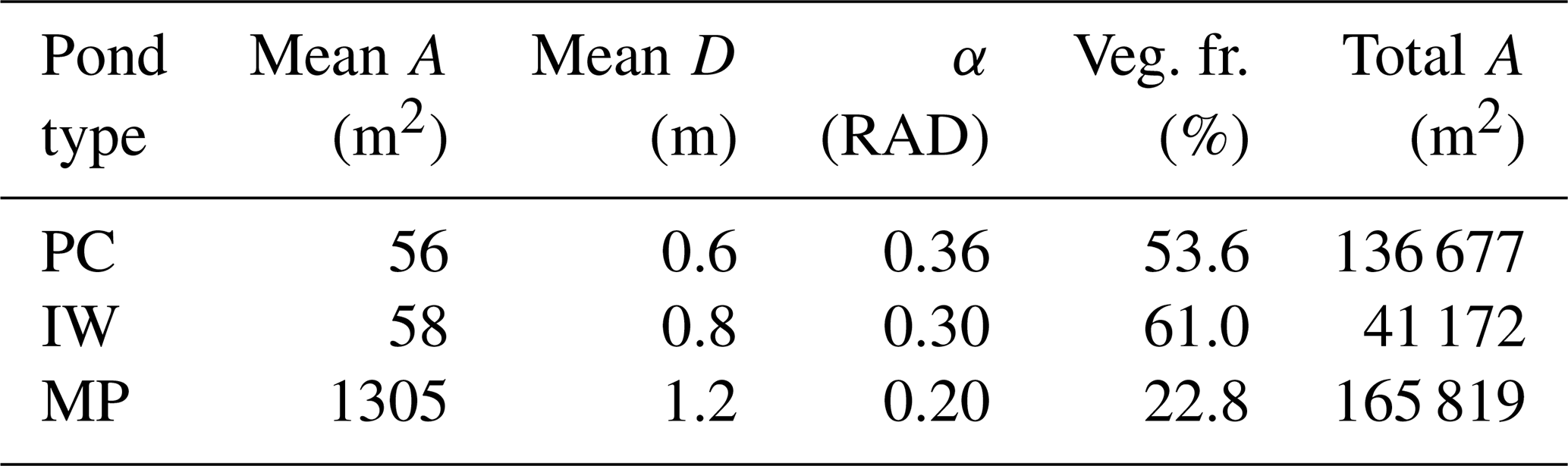
Table 1 Properties of thermokarst ponds on the river terrace of Samoylov Island. Ponds in MeEP are classified as either polygonal-center (PC), ice-wedge (IW), or merged polygonal (MP) ponds. Each of these types is represented by their typical geometry: the average area of an individual pond (mean A), the total area covered by all ponds of a specific type (total A), and the overgrown fraction of a pond type (veg. fr.) were provided by the land-cover classification (Beckebanze et al., 2022). The mean depths (mean D) are estimates by Rehder et al. (2021). α is the angle between the bank of the pond and the horizontal plane. Since macrophytes only grow in shallow water, α was set to match the overgrown fraction of each pond type. Ponds cover roughly 11.5 % of the Holocene river terrace of Samoylov Island.

2.1.3 Hydrology

The hydrological model (see Sect. S2) is responsible for water table dynamics fed into FLake and for partitioning of the pond into an overgrown and open-water part for the methane module. Water table dynamics are computed as the balance between precipitation, evaporation provided by FLake, and above- and belowground runoff. Belowground runoff follows Darcy's law, and the soil properties were set according to local hydraulic conductivity measurements by Helbig et al. (2013).

Changes in the water table height lead to changes in the areas of the overgrown and open-water parts of the pond. To compute these changes, we assume the pond's cross-section to be an isosceles trapezoid as a simple geometric form, with an angle α between the slope and the horizontal plane. Plants are assumed to grow in all parts shallow enough (water depths <0.5 m), and α was set so that the allocation to overgrown and open water matches observations (Table 1). The methane module is executed for each part of the pond and uses the respective mean water depth.

2.1.4 Methane

The methane module is separated into two parts: one for the ice-free (see Fig. 1b) and one for the ice-covered season. In summer, the model is built on three main assumptions:

• We assume equilibrium between production and emission of methane in each time step. Under this assumption, all variables become stationary, and time-dependent terms are zero.

• We assume that there is no lateral mixing between the overgrown and the open-water parts of a pond. Thus, we can solve the methane module individually for each part of the pond.

• We assume that the whole water column is well mixed in summer and that the methane concentration throughout the water column is constant.

These assumptions introduce inaccuracies. Due to the first and third assumption, MeEP does not consider any effect of methane storage in the pond, which we assume to be negligible, because of the small water depths and regular mixing of the waterbody. Generally we find that in our simulations, the ponds are completely mixed more than half the time even for ice-wedge ponds and that stratification lasts on average less than half a day before the pond is completely mixed again under present conditions. Under warmer climatic conditions, FLake predicts a further reduction in stratification. Thus, the amount of methane that could accumulate in the stratified water is limited, and stratification most directly impacts the rate of diffusion, only one of the three pathways for methane. Overall, the assumptions distinctly simplify the model, and we can find an analytical solution to our equations.

In MeEP, methane is produced exclusively in the sediment, with the production being dependent on the sediment temperature T_b and thaw depth h_s(Stepanenko et al., 2011) as follows:

$$\begin{array}{}\text{(1)}& \begin{array}{rl}{P}_{{\mathrm{CH}}_{\mathrm{4}}}=& {\displaystyle \frac{P_{\mathrm{0}}}{a}}\cdot q_{\mathrm{10}}^{(T_{\text{b}}-\mathrm{273.15})/\left(\mathrm{10}{}^{\circ }\mathrm{C}\right)}\times (\mathrm{1}-e^{-a{h}_{\text{s}}})\cdot f_{\text{prod}}\\ & \left(\mathrm{mol}{\mathrm{m}}^{-\mathrm{2}}{\mathrm{s}}^{-\mathrm{1}}\right),\end{array}\end{array}$$

with P₀ being the tuned base productivity of the ponds. The methane production depends linearly on the net primary productivity (NPP) through the dimensionless f_prod, which is based on Walter et al. (2001) and was set up to range from zero to roughly one under present-day conditions. Since the methanogens do not use all the substrate within the same time step, we apply a running average on NPP with a window length of 1 month and split methane production into a part dependent on NPP (75 %) and a base productivity (25 %) based on findings by Bouchard et al. (2015) and Dean et al. (2020). Methane productivity in the open water correlates with the amount of littoral vegetation (Juutinen et al., 2003); thus for open water f_prod additionally takes the ratio of overgrown versus open water into account. How quickly the methane production decreases with sediment depth is determined by a (m⁻¹), while q₁₀ is a constant describing the temperature dependence, which was set to 3.4 according to local measurements (Walz et al., 2017).

All the methane produced in a time step is emitted or oxidized in the same time step through one of the three following pathways. First, in the overgrown part of the pond, evading through emergent macrophytes is the most efficient pathway for methane, meaning that most methane produced in the sediment is allotted to this plant-mediated transport based on Walter et al. (1996). The amount of methane transmitted through vascular plants depends on the thaw depth and leaf area index as a measure for the seasonality and density of the vegetation. We assume a fixed fraction of the plant-mediated methane to be oxidized (f_ox=0.2), reducing the methane flux from plants F_plant. The value 0.2 is a conservative estimate based on the work of Turner et al. (2020) and Ström et al. (2005), who measured the oxidation rates of the plant species dominating our study region. We compute the plant-mediated transport as

$$\begin{array}{}\text{(2)}& \begin{array}{rl}{F}_{\text{plant}}=& (\mathrm{1}-f_{\text{ox}})\cdot \text{min}\mathit{\{}\mathit{\beta }\cdot f_{\text{growth}}\cdot h_{\text{s}}\cdot c({\mathrm{CH}}_{\mathrm{4}}{)}_{\text{b}}^{\text{sat}},P_{{\mathrm{CH}}_{\mathrm{4}}}\mathit{\}}\\ & \left(\mathrm{mol}{\mathrm{m}}^{-\mathrm{2}}{\mathrm{s}}^{-\mathrm{1}}\right).\end{array}\end{array}$$

β (s⁻¹) is a dimensionless factor describing plant density and their ability to conduct methane combined with a rate factor (Walter et al., 2001); f_growth is a dimensionless measure of the plant growth which depends on the leaf area index, which varies between 0 and 4 and is computed following Walter and Heimann (2000); and $c({\mathrm{CH}}_{\mathrm{4}}{)}_{\text{b}}^{\text{sat}}$ is the saturation concentration of methane in the sediment, which we compute using temperature-dependent Henry constants ($H_{\text{b}}^{{\mathrm{CH}}_{\mathrm{4}}}$ and $H_{\text{b}}^{{\mathrm{N}}_{\mathrm{2}}}$). The concentration is controlled by the hydrostatic pressure at the pond bottom p_h and the partial pressure of nitrogen (N₂). We assume the N₂ concentration to be in equilibrium with the atmosphere in the water column (c(N₂)_eq) and decay exponentially in the sediment at the rate ${\mathit{\lambda }}_{{\mathrm{N}}_{\mathrm{2}}}$ (Stepanenko et al., 2011; Bazhin, 2001). The saturation concentration then reads

$$\begin{array}{}\text{(3)}& \begin{array}{rl}c({\mathrm{CH}}_{\mathrm{4}}{)}_{\text{b}}^{\text{sat}}=& \mathit{\varphi }\cdot H_{\text{b}}^{{\mathrm{CH}}_{\mathrm{4}}}\cdot \mathit{\gamma }\cdot \left(p_{\text{h}}-{\displaystyle \frac{c({\mathrm{N}}_{\mathrm{2}}{)}_{\text{eq}}}{H_{\text{b}}^{{\mathrm{N}}_{\mathrm{2}}}}}\cdot e^{\frac{-{\mathit{\lambda }}_{N_{\mathrm{2}}}\cdot h_{\text{s}}}{\mathrm{2}}}\right)\\ & \left(\mathrm{mol}{\mathrm{m}}^{-\mathrm{3}}\right),\end{array}\end{array}$$

where ϕ denotes the porosity of the top sediment (m³ m⁻³), which is set to 0.97 based on measurement data (Helbig et al., 2013; Zubrzycki et al., 2013), and γ, a dimensionless threshold which was tuned using chamber measurements of pond methane fluxes by Knoblauch et al. (2015).

Next, methane is diffused through the water column and into the atmosphere. We compute diffusion based on the balance

$$\begin{array}{}\text{(4)}& {\displaystyle }{F}_{\text{b}}^{\text{diff}}-F_{\text{diff}}-F_{\text{ox}}{\displaystyle }=\mathrm{0},\end{array}$$

where $F_{\text{b}}^{\text{diff}}$ and F_diff stand for the methane flux between the sediment and water column and between the water column and atmosphere, respectively. Diffusion is the slowest pathway; thus, we dynamically account for oxidation (F_ox) using the Michaelis–Menten relation with constants determined by Martinez-Cruz et al. (2015). We compute $F_{\text{b}}^{\text{diff}}$ based on the gradient between the concentration in water and sediment multiplied by the diffusivity based on Sabrekov et al. (2017). For diffusion to the atmosphere we utilize

$$\begin{array}{}\text{(5)}& F_{\text{diff}}=k_{\text{p}}\left(c({\mathrm{CH}}_{\mathrm{4}}{)}_{\text{aq}}-c({\mathrm{CH}}_{\mathrm{4}}{)}_{\text{aq}}^{\text{eq}}\right)\left(\mathrm{mol}{\mathrm{m}}^{-\mathrm{2}}{\mathrm{s}}^{-\mathrm{1}}\right)\end{array}$$

and compute the piston velocity k_p following Heiskanen et al. (2014). The water methane concentration is denoted by c(CH₄)_aq, and $c({\mathrm{CH}}_{\mathrm{4}}{)}_{\text{aq}}^{\text{eq}}$ is the methane concentration if the water column were in equilibrium with the atmosphere. We solve Eq. (4) for c(CH₄)_aq to compute the fluxes.

Lastly, if more methane is produced than what can leave the sediment through plant-mediated transport or diffusion, this methane escapes the ponds in the form of gas bubbles (ebullition).

We assume that there is no exchange of methane between the water column and atmosphere, while the pond is ice-capped in winter. However, methane is still produced in the sediment until it freezes during the ice-on period. This methane accumulates in the water column, where part of it oxidizes until the oxygen in the water column is depleted. Furthermore, if methane concentrations exceed the temperature-dependent saturation concentration, the methane gasses out. This methane is encapsulated in the ice (Langer et al., 2015). The methane accumulated in the water column and the methane caught in the ice are emitted at once when the ice cover comes off. For simplicity the ice cover is not fractional, so the pond is either ice-covered or has no ice.

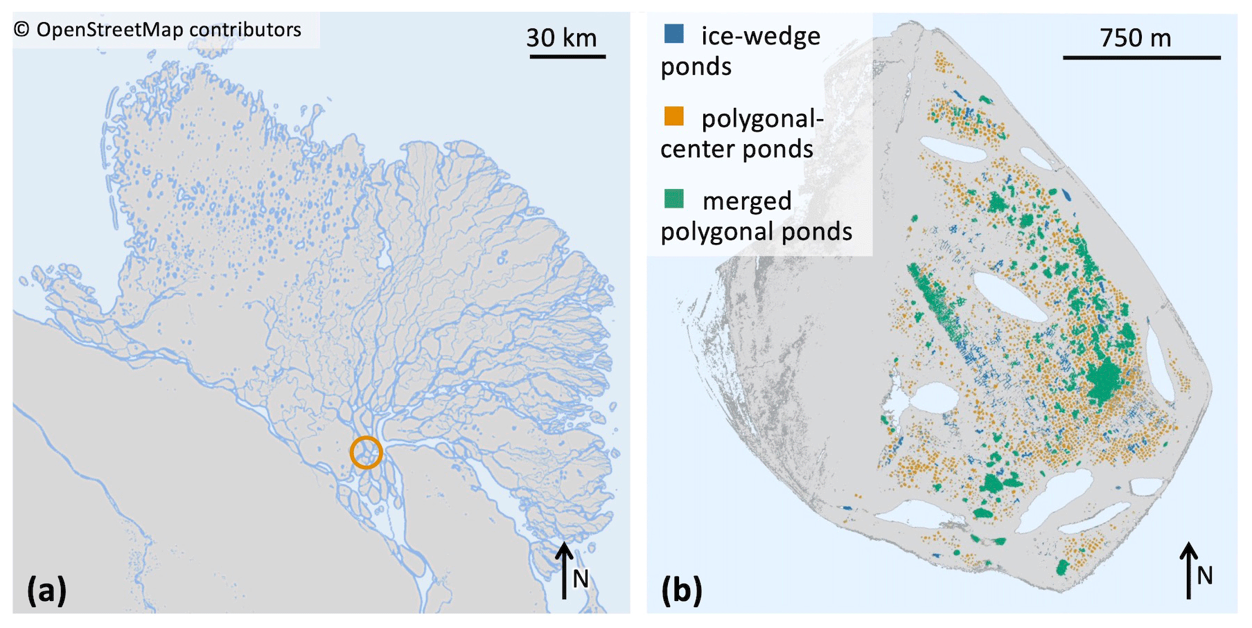
Figure 2 (a) Map of the Lena River delta, which is situated in northeastern Siberia. Location of Samoylov Island marked by a circle. © OpenStreetMap contributors 2022. Distributed under the Open Data Commons Open Database License (ODbL) v1.0. (b) Map of Samoylov Island including a classification of all ponds on the river terrace (eastern part of the island) based on the landscape-scale pond classification. Larger lakes which are not part of this study are drawn in light blue.

2.2 Study site in the Lena River delta

In this study we focus on the extensively researched Samoylov Island (Kutzbach et al., 2004; Abnizova et al., 2012; Helbig et al., 2013; Zubrzycki et al., 2013; Knoblauch et al., 2015; Boike et al., 2019; Rehder et al., 2021; and Beckebanze et al., 2022; among others). Samoylov Island lies in the Lena River delta of northeastern Siberia at 72^∘22^′ N and 126^∘30^′ E (Fig. 2). The island is composed of Holocene sediments and can be divided into two geomorphologically different parts. The western part consists of a floodplain, while the eastern part is a river terrace featuring polygonal tundra (Zubrzycki et al., 2013; Kartoziia, 2019). This part of the island contains more than 1300 ponds (Muster et al., 2012) in an area of ∼3 km² (Beckebanze et al., 2022) and thus is an excellent site to study ponds. Surface methane concentrations in the different pond types are similar to polygonal-tundra ponds in Canada (Rehder et al., 2021). We use a pond classification (Mirbach et al., 2022) which provides spatial information on the location, size, and type of all ponds on Samoylov Island (Table 1 and Fig. 2b). This classification uses the distinct shapes and sizes of the three pond types to distinguish between the three pond classes. The pond types are determined by size limits and by how circular the pond is.

2.3 Forcing and setup of scenario simulations

To force MeEP, we use a mixture of reanalysis (ERA5; Hersbach et al., 2020) and remote-sensing (MODIS; Myneni et al., 2015) data: we use the ERA5 variables for specific humidity, surface downwards solar radiation, surface downwards thermal radiation, surface pressure, temperature at 2 m height, total precipitation, and the wind speed at 10 m height. Wind speed has been computed as the Euclidean norm of two orthogonal wind components. From MODIS, we extract the leaf area index for low vegetation and estimate net primary production. Net primary production is calculated as half of the gross primary production (Waring et al., 1998; Gifford, 2003). We always extract the grid box closest to our study site for 2002–2019. To spin up MeEP, we compute the average year from this period and force MeEP for 10 years with this average forcing. For analysis, we use the years 2004–2019. At the beginning of 2004, the vegetation cover is reset once.

Table 2 Overview of warming simulations. The simulations (sim.) we conduct are listed in this table. We use historical forcing for the hist_all simulations, and for the experiments we use forcing adapted to a mean increase in annual temperature ΔT.

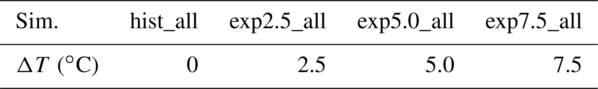
In addition to a historical simulation hist_all, we simulate warming scenarios. To that end, we scale each forcing variable to fit a ΔT warmer Arctic, with $\mathrm{\Delta }T\left({}^{\circ }C\right)\in \mathit{\{}\mathrm{2.5},\mathrm{5},\mathrm{7.5}\mathit{\}}$ (exp2.5_all, exp5.0_all, and exp7.5_all). Due to the Arctic amplification, we might reach a warming of 7.5 ^∘C even under moderate warming scenarios. Thus, by choosing evenly spaced temperature increases with a maximum warming of 7.5 ^∘C, we track how emissions are likely to change in the future (Bekryaev et al., 2010; Rantanen et al., 2022). We determine expressions to scale the forcing variables using the Max Planck Institute Earth system model (MPI-ESM) simulations (Wieners et al., 2019; Mauritsen et al., 2019) from the 1pctCO2 scenarios of CMIP6 (Eyring et al., 2016). We fit each variable to the local annual mean temperature for each month, either linearly or with a quadratic function. If the slope of the fit exceeds its standard deviation (i.e., the change is significant), we scale the forcing variable. No trend was detected for wind speed, shortwave radiation, and air pressure. We adapted net primary productivity, the leaf area index, incoming longwave radiation, precipitation, relative humidity, and air temperatures. Using the fit, we can compute a monthly change in the forcing for a given temperature increase ΔT. We interpolate linearly between two values to apply this monthly increase to hourly time steps. In the MPI-M 1pctCO2 simulation, our study area warms about 2.1 times faster than the global average. Thus, our local warming scenarios of 2.5, 5, and 7.5 ^∘C correspond to moderate global temperature increases of 1.2, 2.4, and 3.6 ^∘C compared to present temperatures.

Table 3 Additional simulations to extract the signal from individual components. We force the methane module with mixed forcing from the hist_all and exp5.0_all simulations, separating three components based on (a) temperature- and season-length-related variables (exp5.0_Temp), (b) variables connected to hydrology (exp5.0_Hyd), and (c) variables representing vegetation (exp5.0_Veg).

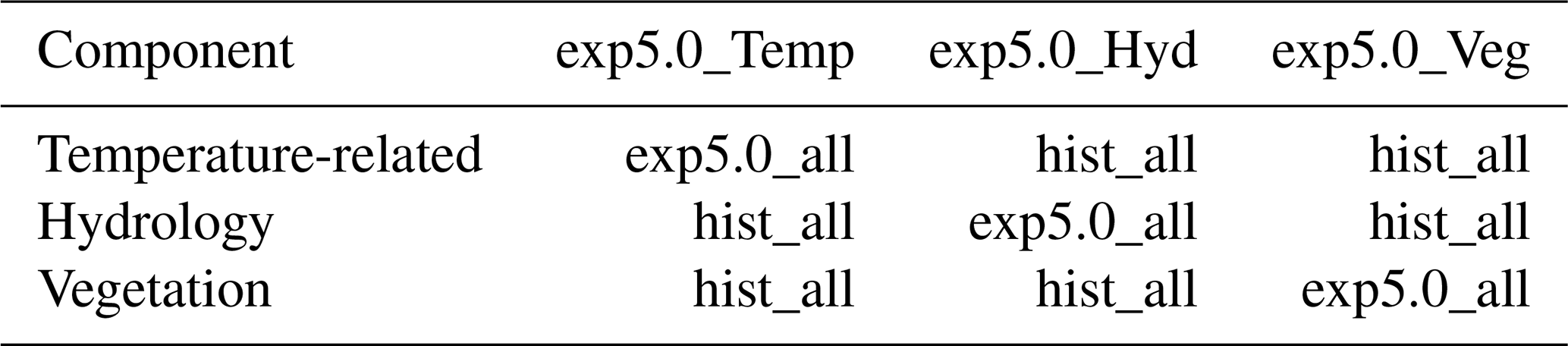
Temperature-related variables: thaw depth, Deardorff velocity, pond mixed-layer and bottom temperature, ice thickness, and its changes since the last time step. Hydrology: areas and mean depths of the overgrown and open-water parts of the ponds. Vegetation: leaf area index and net primary productivity.

Lastly, to extract the impact of specific components on the pond methane emissions, we simulate the methane module with mixed forcing from hist_all and exp5.0_all (Table 3). The components we extract are (a) temperature- and season-length-related variables (exp5.0_Temp), (b) variables connected to hydrology (exp5.0_Hyd), (c) and variables representing vegetation (exp5.0_Veg). Since mixing the forcing of the historical simulation and the warming scenario simulations leads to artifacts in spring and fall, when ice is about to melt or has just formed, we do not account for the spring flush in these simulations. Thus, we only focus on open-water-season emissions.

Table 4 Tuning parameters. The parameters listed below were set using data by Knoblauch et al. (2015).

3 Model tuning and validation

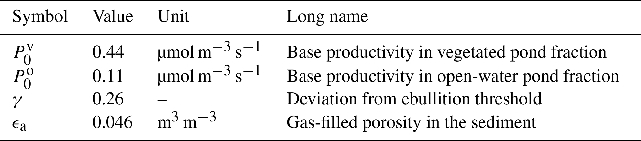
The base productivity in the sediment and the distribution of methane among the three pathways were tuned using chamber measurements by Knoblauch et al. (2015). Their dataset provides time series of the individual methane pathways for five ponds – four polygonal-center ponds and one ice-wedge pond – on Samoylov Island during two seasons. In total, six variables were tuned (Table 4). We tuned the general magnitude of the fluxes using the base productivity P₀ (Eq. 1) and tuned it separately for the overgrown and the open-water part of the pond. γ is a factor used to determine the saturation concentration in the sediment, which uses Henry's law (Eq. 3). It is introduced as a correction factor to account for the shape of the bubbles; Henry's law was derived for flat surfaces, but bubbles are spherical (Stepanenko et al., 2011). We also tuned the gas-filled porosity in the sediment, for which no measurements were available. This parameter influences the diffusion from the sediment into the water column (Sabrekov et al., 2017).

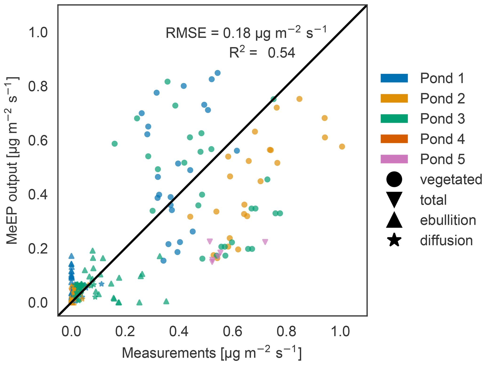
Figure 3 Measured versus tuned modeled methane emissions. Comparison of measured (x axis) and modeled (y axis) methane fluxes for the five ponds measured by Knoblauch et al. (2015) (color code). The fluxes are broken down into different pathways (ebullition and diffusion) where possible. Vegetated fluxes are fluxes measured over the overgrown part of the pond.

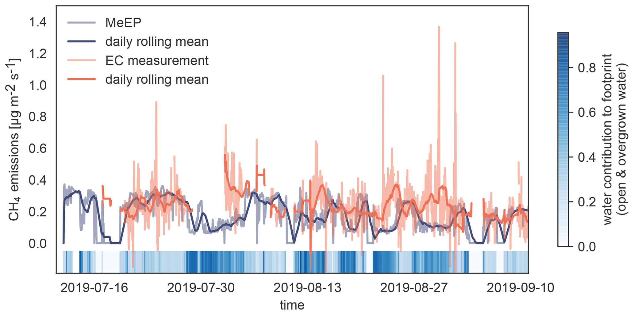
Figure 4 Validation of MeEP with eddy covariance (EC) measurements. We compare the EC flux measurements (Beckebanze et al., 2022) to simulated EC flux using the overgrown and open-water fluxes modeled with MeEP and the measured mean tundra fluxes of 0.15 µg m⁻² s⁻¹ multiplied by their respective contribution to the footprint. The eddy covariance measurements were then taken to a large merged polygonal pond. To visualize how much the pond contributed to the flux in a time step, we added colored strips at the bottom of the plot.

When comparing the individual flux measurements against modeled values (Fig. 3), we achieved an R² value of 0.54, and thus the model is able to capture the average behavior of the ponds. Much of the variance can in part be explained by differences between ponds. The tuning parameters are the overall best fit, but not necessarily the best fit for each pond, so that some fluxes are over- and some are underestimated. Notably, the maximal goodness of the fit we can achieve depends on the q₁₀ value we use. We set q₁₀ to 3.4 to match local measurements (Walz et al., 2017). Jansen et al. (2022) synthesized measurements of methane production in global lake sediments and determined the temperature dependency using an Arrhenius-type equation. In the temperature range of our simulations, using a q₁₀ of 3.4 is in the range of the uncertainty of Jansen et al. (2022) (see Fig. S3). However, if we use a q₁₀ of 2 and tune the model again, we achieve a better match between the model and measurements (R² value of 0.63; see Fig. S4). This indicates either that the temperature dependence of methane production is lower than 3.4 or that we underestimate the temperature dependency of methane-consuming processes along the different emission pathways. However, both tuned model versions, with a q₁₀ of 2.0 and of 3.4, have a similar annual cycle (Fig. S5a) because we tune the magnitude of summer emissions to measurements. Nevertheless, the spread between total annual emissions is larger when using a higher q₁₀ (Figs. S5b and S6), and the standard deviation in the estimate by Walz et al. (2017) can lead to a doubling or halving in total emissions if the model is not tuned again (Fig. S6). This shows that the measurement uncertainty regarding the temperature dependence of methane production translates into large uncertainty regarding modeled methane emissions if the modeled emissions are not constrained by further measurements.

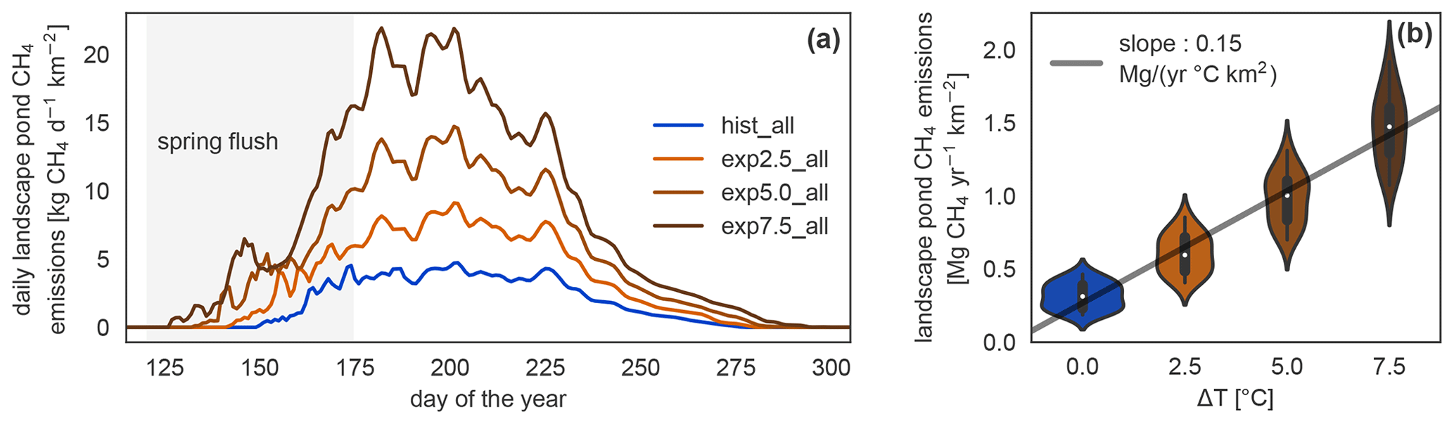
Figure 5 Daily and annual methane emission changes in the different simulations. (a) Seasonal dynamics of methane emissions from ponds per square kilometer of river terrace on Samoylov Island in scenario simulations. The seasonal cycle exhibits a peak at the beginning of the open-water season caused by the spring flush. (b) Linear regression of annual landscape-scale pond methane emissions per square kilometer of river terrace versus annual mean temperature increase. The distribution of annual emissions per year in each simulation is depicted as violin plots: the more often a certain y value occurs, the wider the shape is.

To assess how well the model performs compared to measurements to which it has been tuned, we use eddy covariance measurements from Samoylov Island from summer 2019 (Beckebanze et al., 2022). Eddy covariance fluxes are almost always a compound of fluxes from different land cover classes. In this case, the footprint, the area measured by the eddy covariance instruments, includes mostly tundra to the west interspersed with polygonal-center ponds, which make up about 10 % of the footprint in this wind direction. To the east, over 90 % of the footprint of the tower consists of the open and overgrown water of the merged polygonal pond. The relative contribution of the three surface classes, open and overgrown water and tundra, to the eddy covariance flux varies with time, and a pure signal from the waterbody does not exist. To compare MeEP to measurements, we imitate the eddy covariance signal using the contribution of each of the three surface classes to the footprint. This contribution was retrieved using a footprint model and a land cover classification (Mirbach et al., 2022). The overgrown and open-water fluxes predicted by MeEP are multiplied by their respective cover fraction. To this end, we add the mean tundra flux determined with the eddy covariance method of 0.15 µg m⁻² s⁻¹ and then compare this simulated eddy covariance flux to the real eddy covariance fluxes (Fig. 4). Please refer to Beckebanze et al. (2022) for more detail on the data processing.

MeEP-based fluxes are slightly lower, so MeEP output might be a conservative estimate of landscape pond methane emissions. However, there are some differences in temporal development. The spatial heterogeneity likely causes these differences in the measured fluxes, which MeEP cannot reproduce. Seep ebullition (constant ebullition from one spot) likely generated especially high emissions from one point in the measurements. In the simulated fluxes, ebullition is assumed to be constant over the area. Thus, differences in the temporal evolution are expected, and we conclude that the tuning of MeEP was successful.

We want to note that MeEP was designed for an average pond, not for individual ponds. Methane emissions from individual waterbodies can be highly variable (Sepulveda-Jauregui et al., 2015; Jansen et al., 2020; Beckebanze et al., 2022). However, MeEP provides emission estimates for an average pond rather than resolving spatial heterogeneity within a pond.

4 Results

4.1 Methane emission response to warming

MeEP projects an increase in methane emissions with warming (Fig. 5), from methane emissions of (316±86) kg CH₄ yr⁻¹ km⁻² (mean and standard deviation) in the hist_all simulation to (605±128), (985±172), and (1466±232) kg CH₄ yr⁻¹ km⁻² in the exp2.5_all, exp5.0_all, and exp7.5_all simulations, respectively. These are the average river terrace emissions using an area-weighted mean of the three pond types. Emissions in the exp5.0_all simulation are 3.1 times higher than in the hist_all simulation. Using a linear regression between the mean increase in annual air temperature and the total pond emissions (Fig. 5b), we determine an increase in emissions from pond areas of 1.33 g CH₄ yr^−1 ∘C⁻¹ m⁻². The increase in annual emissions is caused by an increase in mean emissions over the open-water season and by a longer open-water season (Fig. 5b). The open-water season lengthens from a mean of 109 d in hist_all to 124 d in exp2.5_all, 138 d in exp5.0_all, and 152 d in exp7.5_all. On average, the growing season lengthens by 5.7 d ^∘C⁻¹ of warming.

We further investigate the interaction of increased season length and elevated temperatures using growing-degree days. The accumulated growing-degree days above 5 ^∘C (GDD5) integrate temperatures and season length in one metric. The annual methane emissions exhibit a clear linear dependence on GDD5 (Fig. 6). This linear dependence, however, does not hold for all simulations. The differences between the applied forcings cause offsets between the different experiments. While the forcing itself uses ERA5 and MODIS, we used ESM scenario simulations to determine the forcing variable's sensitivity to warming. We find a strong dependence, especially of net primary productivity on warming in the ESM simulations, leading to pronounced changes in this variable across MeEP simulations. If 2 years, 1 from the hist_all simulation and 1 from exp2.5_all, have a similar mean annual air temperature, then net primary productivity in the exp2.5_all simulation will exceed primary productivity in the hist_all simulation by more than 60 %. Thus, air temperature can only be used as a proxy for other forcing variables within one simulation, not across simulations with different forcing. However, air temperature or GDD5 can predict total pond methane emissions within one simulation. Note that, in contrast to Fig. 5, the emissions displayed in Fig. 6 are not integrated over the total pond area on Samoylov Island but are given in relative units per pond area. Thus, we do not account for changes in the pond area.

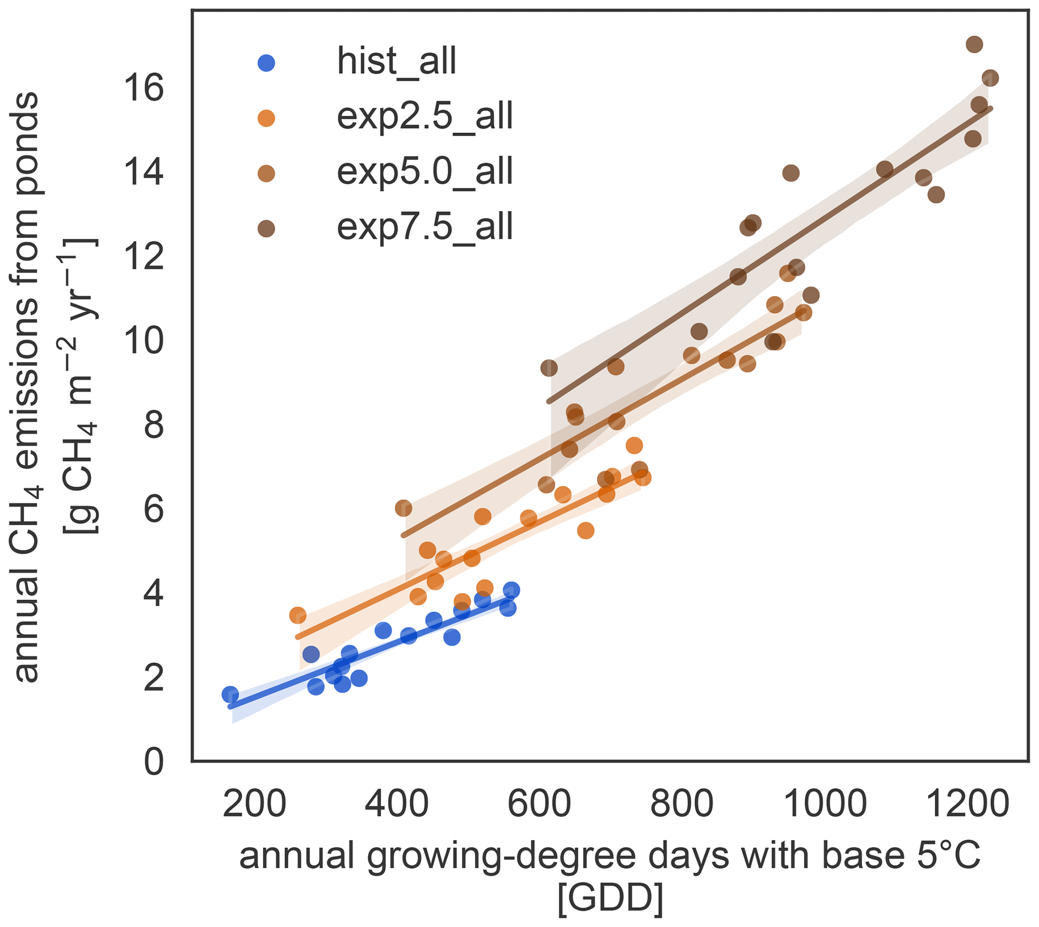
Figure 6 Growing-degree days as a control on annual methane emissions. For each simulation, the dependence of the cumulative annual methane emissions (y axis) on the cumulative annual GDD5 (x axis) can be approximated by a linear regression (solid lines, confidence intervals shown as shaded area).

4.2 Hydrological response to warming

The total pond area and its allocation to open and overgrown water change with time between simulations. In MeEP, ponds are initialized at the beginning of the simulation. Though no new ponds can form during a simulation, MeEP computes the water table based on the hydrological budget of precipitation, evaporation, and both below- and aboveground runoff. MeEP projects only a small reduction in the total pond area in response to elevated temperatures (Fig. 7). Even the area reduction in the most extreme warming simulation we conducted (exp7.5_all) is still within the standard deviation of the base simulation hist_all. Total pond areas decrease from a landscape fraction of 11.7±0.4 % (mean ± standard deviation) in the hist_all scenario to 11.5±0.4 % in exp7.5_all. Consequently, the changes in the areas of open and overgrown water are negligible, and on average, 4.7±0.4 % of the landscape is covered by the overgrown water fraction of ponds. However, the hydrological module of MeEP is rather simple, and we examine its limitations in Sect. 5.3.

4.3 What causes the methane emission to increase?

Since the changes in waterbody areas are small, the impact of the hydrology on the total methane emissions is small too. Nevertheless, the decrease in area is the only response of the system which leads to a reduction in the emissions under warming (Fig. 8). Changes in physical variables, like temperature and the length of the open-water season, lead to an increase in emissions with warming. In our simulation, vegetation biomass and productivity increase under elevated temperatures. These changes in vegetation are the dominant driver of increased methane emissions with warming. Though emissions start later in the year in the exp5.0_Veg simulation compared to the exp5.0_Temp simulation, the total annual emissions are much higher than in the simulations which exclude the increased plant productivity. Thus, changes in the forcing related to vegetation are the main driver of methane emission increases.

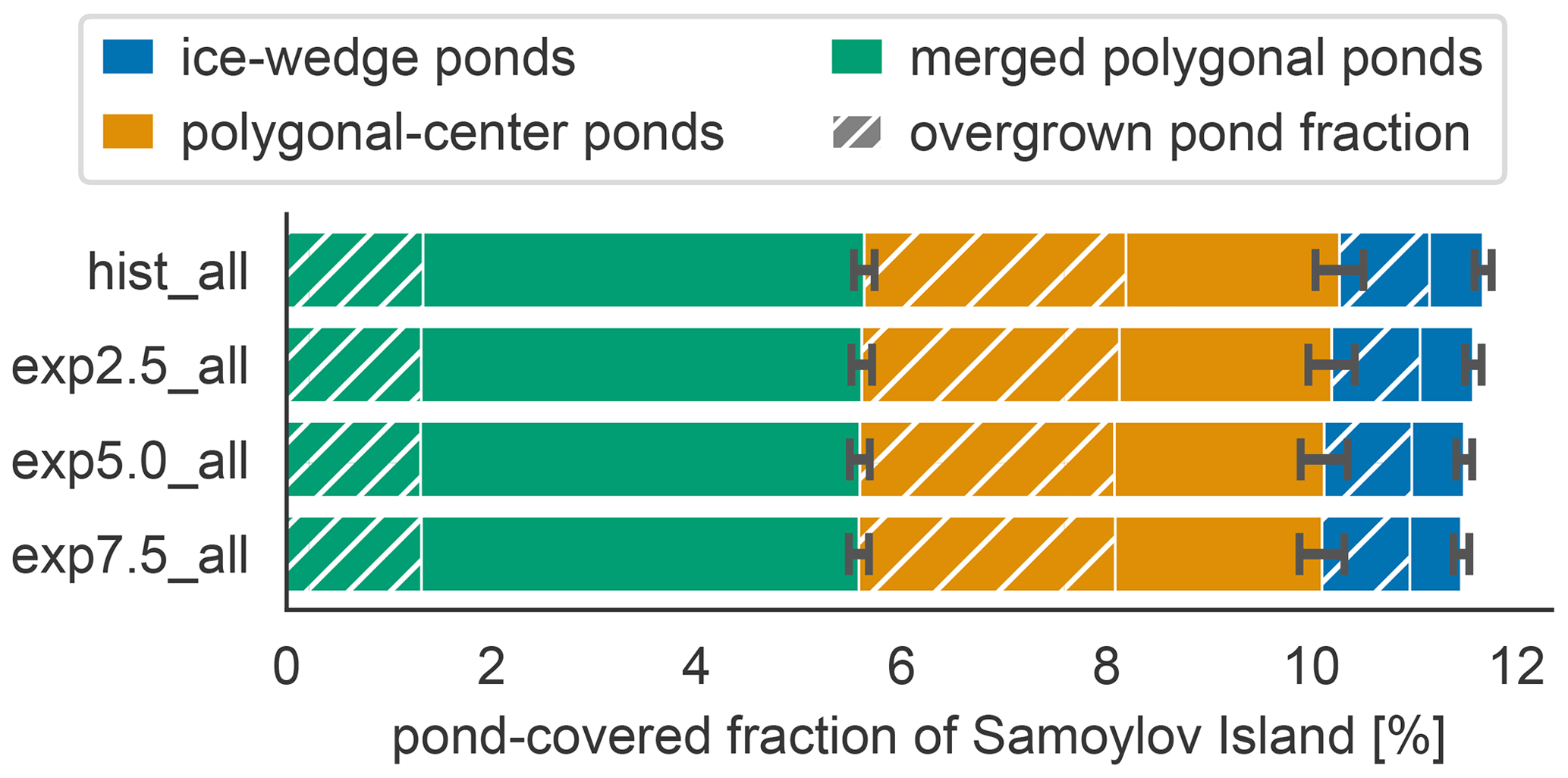
Figure 7 Pond area changes between simulations. The average landscape fraction covered by each pond type (y axis) changes slightly between scenarios (x axis). The overgrown fraction of each pond type is hatched.

Table 5 Methane emissions from each pond type. The open-water season fluxes differ between open and overgrown water for the three pond types. Shown here are values from the hist_all simulation. The total pond fluxes are computed using an area-weighted mean.

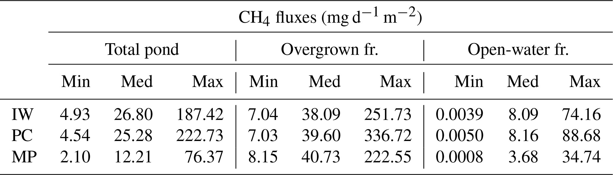
IW, ice-wedge pond; PC, polygonal-center pond; MP, merged polygonal pond; min, minimum; med, median; max, maximum; fr., fraction.

4.4 Impact of pond methane emissions on the landscape scale

The impact of vegetation can also be observed when investigating the impact of overgrown- and open-water fluxes on the landscape scale. While the modeled fluxes from overgrown water exceed the measured average tundra fluxes (Wille et al., 2008), fluxes from open water are lower (Fig. 9a). When comparing simulated emissions from the three pond types to overall tundra emissions measured with eddy covariance (Fig. 9b), we find that ice-wedge and polygonal-center ponds emit slightly more methane per unit area of pond than the average tundra. In contrast, merged polygonal ponds emit slightly less. The latter are the pond type with the highest open-water fraction (Table 5). To summarize, though small ponds contribute slightly disproportionately to the landscape methane emissions, we do not find that ponds are hotspots of methane emissions at the landscape scale – at least not under the current climate.

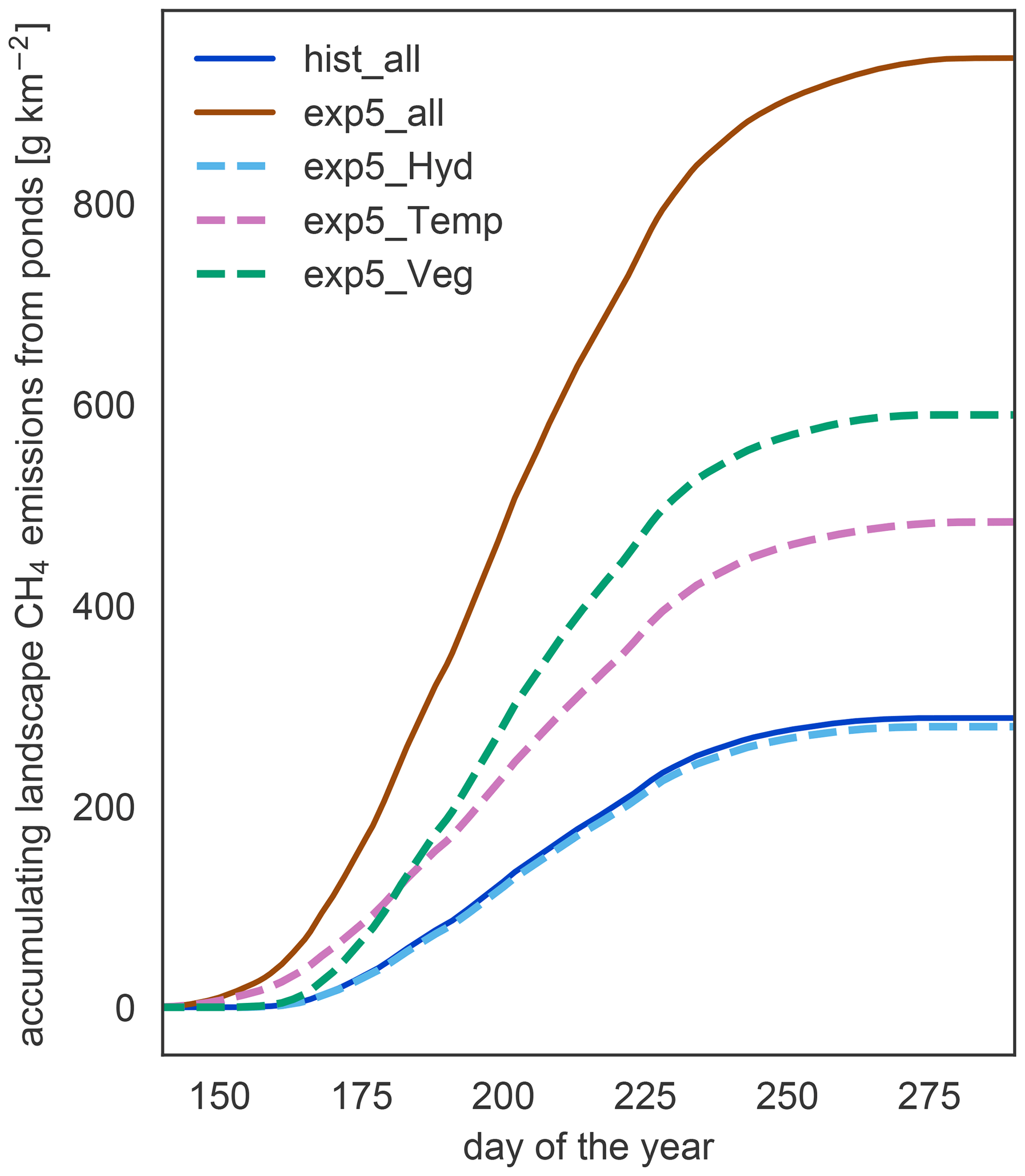
Figure 8 Components driving changes in methane emissions. To isolate the impact of different components on the increasing methane emissions, we simulate the methane part of MeEP mixing input from hist_all and exp5.0_all (see Table 3). In this figure, we compare the accumulated emissions over the course of the average year between different simulations.

Albeit lower than the fluxes from overgrown water in all scenarios, open-water fluxes become more important in the warming simulations (Fig. 10), mostly due to increased ebullition. The relative importance of the plant-mediated fluxes, on the other hand, stays constant over the scenarios, while the impact of the spring flush decreases substantially. In hist_all, the spring flush contributes between 6 %–23 % (minimum and maximum), with a mean contribution of 10 %. In the exp7.5_all simulation, the maximal contribution of the spring flush of 5 % is lower than the minimum contribution in the hist_all simulation. Overall, we find a pronounced increase in pond methane emissions with warming.

5 Discussion

5.1 MeEP model output is conservative compared to pan-Arctic methane flux measurements

Ponds in our study region exhibit low methane emissions compared to other Arctic ponds (Liebner et al., 2011). Emissions from ponds are of a similar magnitude to the overall tundra emissions measured by an eddy covariance system which averages over different surface types (Fig. 9; Beckebanze et al., 2022). MeEP was tuned to local measurements reproducing the typical local emission patterns and predicts median emissions of 12–27 mg d⁻¹ m⁻² depending on the pond type. In a circumpolar synthesis, Kuhn et al. (2021) determined methane emissions from different lake classes. They estimated median diffusive fluxes of 16 mg d⁻¹ m⁻² from small (<0.1 km²) peatland lakes, the class closest to the waterbodies studied here. Adding ebullitive fluxes of 23 mg d⁻¹ m⁻², they estimate total emissions of 39 mg d⁻¹ m⁻² from small peatland lakes. Thus the present-day emissions in our study area are low compared to the pan-Arctic average, and when upscaling to a broader landscape, higher emissions than the ones predicted here can be expected.

The emission patterns of pond types in MeEP are the same as in observational studies. Bouchard et al. (2015) found open-water emissions with a median of 56.6 mg d⁻¹ m⁻² from ice-wedge ponds, 27.9 mg d⁻¹ m⁻² from polygonal-center ponds, and 3 mg d⁻¹ m⁻² from lakes in a polygonal landscape in northeastern Canada in July. As in our model setup, ice-wedge ponds emit only slightly more methane than polygonal-center ponds, and larger waterbodies emit considerably less.

Prėskienis et al. (2021) also measured the spring flush. They estimate that up to 52 % of the annual methane is emitted when the ice melts. This is nearly double our maximum values of 23 %. Wik et al. (2016), who aggregated pan-Arctic fluxes, report an average spring flush of 27 % for thermokarst waterbodies, which is still larger than the mean amount in the hist_all simulation of 10 %. Notably, Wik et al. (2016) summarized waterbodies of all sizes in the thermokarst category, and Prėskienis et al. (2021) reported lower spring flushes for larger waterbodies. Thus, the spring flush modeled by MeEP (Fig. 5) might be a low estimate of the real spring flush but are of the right order of magnitude.

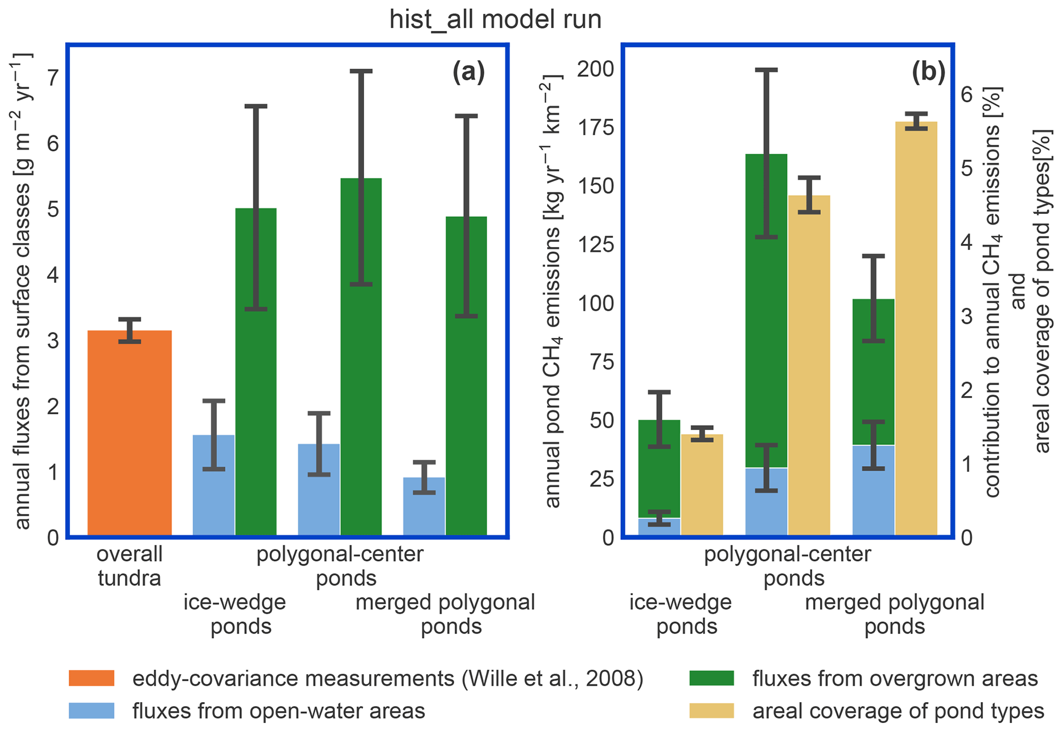
Figure 9 Impact of pond emissions on landscape methane emissions. (a) For the hist_all simulation, we compare fluxes from different landscape elements. The estimates for the overall tundra emissions (orange bar) were acquired with eddy-covariance measurements over the growing season of 2003 (Wille et al., 2008) and are shown for comparison. Note that the influence of ponds on these measurements is low. The methane emissions per square meter of open and overgrown water are broken down per pond type. (b) Methane emissions per square kilometer of polygonal tundra of each pond type are displayed as stacked bars. We compare these emissions per pond type to the area this pond type covers in the polygonal tundra of Samoylov Island (sand-colored bar). This comparison relies on the assumption that the emissions measured by Wille et al. (2008) are representative of polygonal-tundra emissions.

Pond methane emissions from our study site are lower than emissions measured elsewhere, and the spring flush predicted by MeEP is also a lower estimate. So, while pond methane emissions in the hist_all simulation are comparable to measurements in, e.g., the Canadian Arctic, the absolute magnitude of fluxes presented in this study is a conservative estimate compared to pond emissions on the pan-Arctic scale.

5.2 Vegetation changes intensify pond methane emission increases

In the whole Arctic, vegetation has a strong impact on methane emissions (e.g., Joabsson et al., 1999; Andresen et al., 2017; Turner et al., 2020). We can split this impact into two parts. First, vascular-plant productivity increases substrate availability, which increases methanogenesis (Joabsson and Christensen, 2001; Kim, 2015). Second, emergent macrophytes are a highly efficient pathway for methane emissions (Knoblauch et al., 2015).

Plant-mediated transport means gases diffuse with low resistance through the aerenchyma of plants. Aerenchyma are air-filled pores in leaves, roots, and stems of macrophytes (Whiting and Chanton, 1992; Colmer, 2003). The methane flux through these plants increases with their aboveground biomass (Ström et al., 2012; Joabsson and Christensen, 2001), and the aboveground biomass correlates linearly with leaf area index (Andresen et al., 2017). MeEP uses leaf area index, a variable readily available from remote sensing (Myneni et al., 2015), to modulate the plant-mediated transport (Walter and Heimann, 2000). The leaf area index increases with temperature in our forcing (Euskirchen et al., 2009). This trend is in line with findings that emergent macrophytes, for example Arctophila fulva, have already become more abundant in some regions. Arctophila fulva is a very efficient transmitter of methane (Knoblauch et al., 2015; Andresen et al., 2017), which is also abundant in our study region (Knoblauch et al., 2015). This emergent macrophyte is already expanding in similar landscapes, e.g., on Barrow Peninsula in Alaska (Villarreal et al., 2012). We find that coverage of emergent macrophytes increases in such a way that plant-mediated transport is limited by methanogenesis rather than by the conductivity and abundance of aerenchyma. In overgrown parts of the ponds, plant-mediated transport is by far the dominant mode of transportation (Whiting and Chanton, 1992; Andresen et al., 2017). When comparing open-water and overgrown fluxes, the contribution of the overgrown part stays constant over all scenarios with increasing methane emissions (Fig. 10). The plant-mediated transport scales with the increase in total emissions because the density of vascular plants increases with temperature. We represent the density of plants using leaf area index in the model. A higher density of vascular plants means a higher density of aerenchyma, which increases the capacity of the plant-mediated transport more efficiently. Thus, this capacity builds up at the same rate as methanogenesis.

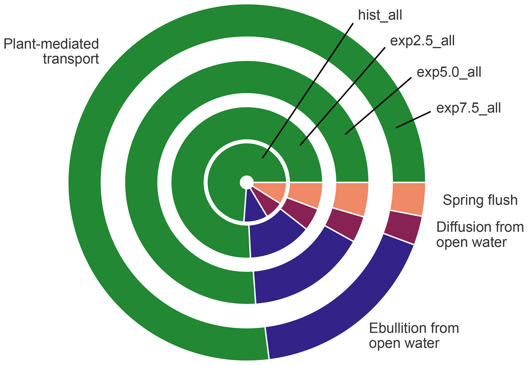
Figure 10 The contribution of each flux type to the overall emissions in the average year. The size of a segment represents the contribution of the respective flux type. The area of each circle is proportional to the absolute methane emissions of the average year in each simulation.

Further, vegetation in permafrost regions adds a positive feedback loop to warming (Lara et al., 2019). Higher temperatures increase plant biomass in the Arctic (Euskirchen et al., 2009; Elmendorf et al., 2012; Andresen and Lougheed, 2015), and, with an increasing thaw depth, conditions for plants become more favorable: nutrients, which are a limiting factor in tundra landscapes, leach out of the thawing permafrost and support vegetation growths (Andresen et al., 2017; Lara et al., 2019). A higher macrophyte cover adds more substrate to the sediment, fueling methanogenesis (Joabsson et al., 1999; Joabsson and Christensen, 2001; Ström et al., 2012; dos Santos Fonseca et al., 2017), which already under present conditions consumes mostly contemporary carbon (Negandhi et al., 2013; Dean et al., 2020). This increases methane emissions, closing the feedback loop (Lara et al., 2019).

In MeEP, this increase in substrate is the main driver of elevated emissions under warming (Fig. 8), leading to an increase in methane emissions that is more than 20 % higher than the increase due to higher temperatures alone. The strength of the methanogenesis response to warming is determined by the term f_prod (see Eq. 1). This term prescribes a linear dependence of methane production on relative changes in net primary productivity. A connection between plant productivity and methanogenesis has been observed in a sub-Arctic fen (Whiting and Chanton, 1992). However, this connection is species-dependent (Vizza et al., 2017; Ström et al., 2005), and some species typical of European wetlands can also reduce methanogenesis (Grünfeld and Brix, 1999). To improve the model, we need additional studies on the impact of emergent macrophytes on Arctic pond or lake methanogenesis.

The linear dependence of methanogenesis on plant productivity is a reasonable first estimate given the evidence that in Arctic landscapes, vascular plants enhance methanogenesis (Joabsson and Christensen, 2001; Ström et al., 2003; Lara et al., 2019). A parameterization based on new measurements that focus on macrophytes' impact in ponds on methanogenesis would be a step forward to constrain future pond methane emissions better. A dynamic model of macrophyte coverage and productivity could be included in a second step. Despite uncertainty in the strengths of the link between methanogenesis and vascular-plant productivity, our projections underpin the importance of future vegetation changes for pond methane emissions.

Vegetation changes occur slowly on multi-annual timescales (Villarreal et al., 2012), leading to higher emissions even in comparably cool years. This effect is especially apparent in Fig. 6; the regressions do not collapse onto a single line. Rather years with the same growing-degree days emit more methane with higher warming. However, growing-degree days are a good predictor of annual methane emissions within a simulation. They combine the direct impact of temperature with a measure of how favorable temperatures are for plant growth for each year. In the Arctic, multi-year vegetation changes are already well underway (Bhatt et al., 2013; Wrona et al., 2016). However, vegetation changes in the Arctic do not solely depend on temperature (Wrona et al., 2016), and the Arctic does not become greener in all regions but even browns in some (Bhatt et al., 2013; Winkler et al., 2021). This browning is strongly connected to changes in hydrology as browning is caused by a lack of water (Winkler et al., 2021).

5.3 Hydrological changes slightly decrease pond methane emission

The tendency of a landscape to become either wetter or drier under warming is dependent on local topography (Jones et al., 2022; Miner et al., 2022). An overall inclined area is likely to drain (Bring et al., 2016). However, in a very flat landscape such as our study area, it might become wetter with warming (Christensen et al., 2004). In the polygonal tundra, warming leads to permafrost degradation, which prompts loss of ground ice, subsidence, and pond formation, leading to higher methane emissions (Kim, 2015), especially along the ice wedges (Yoshikawa and Hinzman, 2003; Liljedahl et al., 2016). Consequently, a degrading polygonal tundra features an increasing number of ice-wedge ponds (Bouchard et al., 2020; Wickland et al., 2020). As the degradation proceeds, the ponds are inclined to vanish again because of either infilling or drainage (Stow et al., 2004; Cresto Aleina et al., 2015; Jorgenson et al., 2015; Wickland et al., 2020). Additionally, an increase in emergent macrophytes can promote pond drainage by intensifying transpiration (Andresen and Lougheed, 2015).

The landscapes drain as permafrost thaws because the disappearing ice has been acting as a barrier for the water. Without permafrost, water can better drain subsurface. However, drainage is impeded if the soils have low permeability, such as highly decomposed peat, and ponds and lakes can be sustained (Smith et al., 2005). Though we do not focus on pond formation in MeEP, existing ponds may drain. MeEP includes a simple surface and subsurface flow formulation, which depends on the local permeability (Helbig et al., 2013). In MeEP, pond areas decrease slightly with warming (Fig. 7). Thus, even in our first-order approximation of pond hydrology, we find evidence of pond drainage reducing pond methane emissions (Fig. 8), though to a lesser extent than for example in van Huissteden et al. (2011). They reported that drainage limits waterbody methane emissions on the landscape scale. The hydrological model implemented in MeEP is one-dimensional and can consequently only provide a first-order estimate of water table dynamics. More complex dynamics on the landscape scale, such as the formation of a network of channels along the ice wedges promoting fast drainage through percolation (Cresto Aleina et al., 2013), are likely to increase drainage. Thus, our estimate of runoff might be too low.

5.4 Landscape-scale impact of pond methane emissions

When estimating the landscape-scale impact of methane emissions from ponds and lakes, many studies concentrate on diffusive emissions (Juutinen et al., 2009; Holgerson and Raymond, 2016; Polishchuk et al., 2018; Hughes-Allen et al., 2021; Zabelina et al., 2020), though some also include ebullition (Sepulveda-Jauregui et al., 2015; Wik et al., 2016; Kuhn et al., 2021). We find that including ebullition is important because, in ponds, ebullition contributes more than diffusion to the total emissions (Kuhn et al., 2021; Praetzel et al., 2021) and becomes much more important with warming (Fig. 10). In MeEP, ponds are very sensitive to rising temperatures. The model projects emissions to roughly double at a temperature increase of only 2.5 ^∘C (Fig. 5b).

Much of the intensification of methane emissions in MeEP is due to vegetation growth, which leads to a strong boost in mean emissions during the ice-free season and a higher peak of emissions in summer (Fig. 5a). These emissions are notably higher than mean tundra emissions already under current climatic conditions (Fig. 9) and should be included in future large-scale pond-methane-emission assessments.

We might even underestimate the response of ponds to warming because methane production is described by a q₁₀ equation (Walz et al., 2017). This description does not account for shifts in methanogen communities, which can enhance the rate of methanogenesis under warming (Zhu et al., 2020). Additionally, we only account for present-day substrate in the current setup; methanogenesis is coupled to vegetation productivity of the same year. This assumption is valid for ponds at the moment (Negandhi et al., 2013; Bouchard et al., 2015; Dean et al., 2020) but might change as permafrost degrades, and old carbon leeches into the ponds (Langer et al., 2015; Prėskienis et al., 2021). This additional carbon is not included in our projections. Therefore, our estimate is conservative.

Our model was set up and calibrated for one specific region featuring one specific landscape type. To quantify emissions in other regions and especially other landscape types, MeEP should be tuned with more and additional data. The magnitude of emissions depends strongly on the base productivity P₀, which is the tuning parameter for the microbial communities and likely differs depending on the structure of the microbial communities. The base productivity for the vegetated pond fraction $P_{\mathrm{0}}^{\text{v}}$ also incorporates the impact of higher substrate availability on the microbial community. Consequently, this parameter is indirectly affected by the vegetation structure in our study region. To apply this model to other regions, special attention should be placed on availability of measurements from the overgrown parts of the ponds, especially plant-mediated transport. One caveat when adapting MeEP for the larger scale is that, in our study area, ponds do not feature floating mosses like sphagnum, which can be found at other sites and reduce methane emissions (Kuhn et al., 2018). While submerged mosses do not impact surface methane concentrations at our study site (Rehder et al., 2021), the same might not be true for floating vegetation.

6 Conclusions

While ponds are not hotspots of methane emissions in our study area under the current climate, our model simulations indicate that they will become stronger methane sources under further warming. We project an increase in pond methane emissions of 1.33 g CH₄ m⁻² yr^−1 ∘C⁻¹. At the same time, the pond area decreases only slightly. However, the hydrological module of MeEP only gives a first-order approximation of water table dynamics. To better gauge the future impact of ponds, we need better projections of pond inception and drainage.

Much of the methane emission increase from ponds is mediated through macrophytes. The vascular plants become more productive and provide additional substrate for methanogenesis. In our simulations, the impact of the additional substrate on methanogenesis is substantially stronger than the impact of elevated temperatures or a prolonged open-water season. However, the relationship between emergent-macrophyte productivity and methanogenesis in ponds could only be approximated due to a lack of measurement data. We further find that plant-mediated transport is the methane pathway contributing most to the overall landscape emissions in simulated-temperature regimes. Unfortunately, plant-mediated transport is the methane pathway least often reported in measurement datasets of pond methane emissions. This makes it harder to generalize our findings at a larger scale, and more observations of this emission pathway and its contribution to overall pond methane emissions are needed. Additionally, the current version of MeEP only uses one value for the conductivity of plants, even though we know that different plant species conduct methane with varying efficiency (Knoblauch et al., 2015). To upscale the plant-mediated fluxes realistically, vegetation maps of the dominant macrophytes would be a strong asset. However, we suppose that vegetation similarly impacts ponds in other Arctic regions. In that case, it is crucial to include macrophytes as a substrate source and as an efficient methane pathway for a pan-Arctic assessment of pond methane emissions under warming.