the Creative Commons Attribution 4.0 License.
the Creative Commons Attribution 4.0 License.
 | 17 Aug 2023
Anthropogenic activities significantly increase annual greenhouse gas (GHG) fluxes from temperate headwater streams in Germany
Ricky Mwangada Mwanake
Gretchen Maria Gettel
Elizabeth Gachibu Wangari
Clarissa Glaser
Tobias Houska
Lutz Breuer
Klaus Butterbach-Bahl
Anthropogenic activities increase the contributions of inland waters to global greenhouse gas (GHG; CO2, CH4, and N2O) budgets, yet the mechanisms driving these increases are still not well constrained. In this study, we quantified year-long GHG concentrations, fluxes, and water physico-chemical variables from 28 sites contrasted by land use across five headwater catchments in Germany. Based on linear mixed-effects models, we showed that land use was more significant than seasonality in controlling the intra-annual variability of the GHGs. Streams in agriculture-dominated catchments or with wastewater inflows had up to 10 times higher daily CO2, CH4, and N2O emissions and were also more temporally variable (CV > 55 %) than forested streams. Our findings also suggested that nutrient, labile carbon, and dissolved GHG inputs from the agricultural and settlement areas may have supported these hotspots and hot-moments of fluvial GHG emissions. Overall, the annual emission from anthropogenic-influenced streams in CO2 equivalents was up to 20 times higher (∼ 71 kg CO2 m−2 yr−1) than from natural streams (∼ 3 kg CO2 m−2 yr−1), with CO2 accounting for up to 81 % of these annual emissions, while N2O and CH4 accounted for up to 18 % and 7 %, respectively. The positive influence of anthropogenic activities on fluvial GHG emissions also resulted in a breakdown of the expected declining trends of fluvial GHG emissions with stream size. Therefore, future studies should focus on anthropogenically perturbed streams, as their GHG emissions are much more variable in space and time and can potentially introduce the largest uncertainties to fluvial GHG estimates.
- Article
(6723 KB) - Full-text XML
- BibTeX
- EndNote


Streams and rivers cover only a small fraction of the earth's land surface (0.4 %; Allen and Pavelsky, 2018), yet they are significant contributors to global greenhouse (CO2, CH4, and N2O) budgets, emitting approximately 7.6 (6.1–9.1) Pg-CO2 equivalent into the atmosphere per year (Li et al., 2021). Headwater streams are hotspots for greenhouse gas (GHG) emissions within fluvial ecosystems due to their large surface area to volume ratio compared to larger rivers, allowing for close connectivity with GHG sources (Hotchkiss et al., 2015; Turner et al., 2015). Several biogeochemical processes are responsible for GHG production and consumption within headwater ecosystems. Biogenic CO2 production is mainly attributed to the respiration of organic matter (Battin et al., 2008). Production of CH4 occurs through methanogenesis, with carbon dioxide and acetic acid as substrates under anaerobic conditions (Stanley et al., 2016). Methane consumption is also possible through methanotrophy in oxygen-rich stream waters, producing CO2 (Shelley et al., 2014). N2O is mainly a byproduct in nitrification (under aerobic conditions) or an intermediate product in denitrification (under anaerobic conditions), but it can also be reduced to N2 in organic-rich and nitrate-poor ecosystems (Quick et al., 2019). Apart from instream biogeochemical production, GHG concentrations in headwater streams may also come from external sources such as groundwater and terrestrial soils (e.g., Borges et al., 2015; Hotchkiss et al., 2015). These external sources are generally dominant during periods of heavy precipitation when the hydrological connectivity between the streams and their surrounding terrestrial landscape and groundwater is activated. Yet, partitioning the sources of these GHGs between in situ production and external sources remains a challenge to aquatic scientists, as their contributions are mainly compounded and also vary widely depending on discharge conditions and the surrounding land use (e.g., Aho and Raymond, 2019; Borges et al., 2019; Mwanake et al., 2022).
Within headwaters, anthropogenic practices such as fertilizer application and construction of drainage ditches to allow agricultural use of former wetlands alter the rates of instream GHG production and their external sources, thereby influencing their spatial-temporal dynamics (Peacock et al., 2021a; Wallin et al., 2020; Mwanake et al., 2019). Elevated hydrological inputs of dissolved GHGs, nutrients, and labile carbon to streams from fertilized croplands have been shown to increase their N2O (e.g., Beaulieu et al., 2009; Mwanake et al., 2019), CO2 (e.g., Bodmer et al., 2016; Borges et al., 2018), and CH4 fluxes (e.g., Deirmendjian et al., 2019; Mwanake et al., 2022) by favoring instream GHG production processes and also ensuring steady supplies in periods of low in situ biogeochemical production. While such trends in agricultural streams show similarities across different catchment locations, GHG emissions from streams in predominantly forested catchments with minor influences from croplands and wetlands show more diverse patterns. Some studies indicated that forest streams are hotspots for GHG fluxes (e.g., Wallin et al ., 2018; Audet et al., 2019; Herreid et al., 2021), while others found the opposite, with much lower fluxes in forests as compared to other land uses (e.g., Bodmer et al., 2016; Mwanake et al., 2022). Besides draining CH4- and CO2-rich terrestrial soils, drainage ditches are characterized by short water residence times, high organic loads, and highly variable O2 levels, which can simultaneously support vigorous CH4 and CO2 production and, subsequently, higher fluxes. For example, in a recent meta-analysis, ditches and canals accounted for up to 3 % of the global anthropogenic CH4 emissions (Peacock et al., 2021b). Yet, studies on them are scarce, and thus the main factors making them hotspots of carbon fluxes are still not well constrained.
In fluvial ecosystems within settlement areas, point-source inflows of wastewater effluents have also been reported to alter natural GHG trends along the river continuum (Park et al., 2018). The wastewater effluent is either substrate-rich, favoring in situ GHG production, or GHG-rich, resulting in high riverine GHG emissions downstream of the inflow point (e.g., Marescaux et al., 2018; Begum et al., 2021; Zhang et al., 2021; Wang et al., 2022). For example, in a study of urban-impacted rivers in the Seine basin in France, Marescaux et al. (2018) found elevated CO2, CH4, and N2O concentrations and fluxes downstream of wastewater inflows, which disproportionately contributed up to 52 % of the basin-wide annual GHG fluxes. Similar findings were also found in urban-impacted rivers in China, where their GHG emissions were up to 14 times higher than those in other land uses (Zhang et al., 2021). Yet, studies on GHG emissions from urban-impacted fluvial ecosystems are still scarce, and therefore their contributions to riverine annual GHG budgets are not well constrained. Moreover, little is known about the cumulative effects of diffuse and point pollution sources on the magnitude of riverine GHG fluxes and whether the diffuse pollution sources exert longer-lasting controls on their fluxes than the point sources.
Under temperate climatic conditions, pronounced seasonality regulates the availability of nutrients and, to some extent, the O2 in lotic ecosystems, which are both key factors driving instream GHG production and gas exchange rates (Borges et al., 2018; Rocher-Ros et al., 2019; Herreid et al., 2021; Aho et al., 2022). Cold winter periods are generally characterized by low instream carbon and nitrogen processing, which results in nutrient accumulation (e.g., Herreid et al., 2021). In contrast, high instream C and N processing are characteristic of warm summer periods (e.g., Borges et al., 2018; Aho et al., 2021, 2022). Seasonality in precipitation regulates discharge, whereby heavy precipitation events or snowmelt during spring result in high discharge events. At the same time, dry summers and winter periods are often characterized by lower discharge (e.g., Aho et al., 2022). Discharge determines the water residence times in streams, which control the rates of instream C and N processing. Previous studies have shown that low discharge periods with longer water residence times favor instream GHG production processes (e.g., Borges et al., 2018; Mwanake et al., 2022). In comparison, high discharge periods with shorter water residence times are unfavorable to instream C and N cycling, resulting in the dominance of externally sourced GHGs from upstream terrestrial sources depending on the surrounding land use. For example, studies have found that during high discharge periods, streams draining wetlands show peak CO2 and CH4 concentrations (e.g., Aho et al., 2019; Borges et al., 2019), and pronounced N2O concentrations are found in streams of cropland-dominated catchments (e.g., Mwanake et al., 2022).
The dynamic interactions between seasonality and land use discussed above indicate that less frequent measurements of riverine GHG concentrations and fluxes may fail to capture periods of elevated fluvial emissions at spatial hotspot areas, resulting in an underestimation of the annual emissions. Yet, only a handful of studies in temperate streams have assessed the seasonal dynamics of GHG fluxes at sampling points with contrasting land uses (e.g., Marescaux et al., 2018; Borges et al., 2018; Herreid et al., 2021; Galantini et al., 2021), resulting in uncertainties in the mechanisms that drive either hot periods or hotspots of fluvial GHG fluxes. As climate change causes more extreme discharge conditions and as agricultural intensification and settlement areas continue to increase (Winkler et al., 2021), more studies that cover a wide array of land uses, discharge, and temperature conditions are needed to allow for developing a better mechanistic understanding of their effects on fluvial GHG dynamics by unraveling synergistic or antagonistic relationships amongst them. This increased process understanding will form the basis of future mechanistic modeling approaches, which are essential to better predict how fluvial GHG emissions will respond to future climate and land use changes (Battin et al., 2023).
The main objective of this study was to assess the seasonality–land-use relationships of water physico-chemical variables and GHG concentration and fluxes by comparing temperate lotic ecosystems of forests and wetlands with those from more human-influenced agricultural and settlement catchments. To do so, we conducted at least tri-weekly measurements covering a full year of observations and mainly focused on headwater streams (stream orders 1–6), which, despite being hotspots of fluvial emissions, remain currently underrepresented in global GHG datasets (Drake et al., 2018; Li et al., 2021). We hypothesize that catchment land use is the most critical control for stream GHG concentration and fluxes, with higher seasonal variability in human-influenced ecosystems than in natural ones. Moreover, we hypothesized that drainage ditches and headwater streams with wastewater inflow within agricultural and settlement areas are hotspots for GHG emissions, driven by direct dissolved GHG inputs or substrate inputs that favor in situ GHG production.
2.1 Study areas and sampling design
Five headwater catchments in central (Schwingbach), southeast (Loisach), and southwest (Ammer, Goldersbach, and Steinlach) Germany were investigated in this study. The catchments covered a wide range of fluvial ecosystems with different stream orders and land use characteristics (Table 1; Fig. 1). The catchment boundaries for each site were determined based on the most downstream sampling location within each catchment (Fig. 1). Elevation of the Schwingbach catchment (54 km2), located in the central-German state of Hessen, ranges from 176–480 m above sea level (a.s.l.). The catchment has a mixed land use of ∼ 41 % mixed forests, 46 % croplands, 8 % settlement areas, and 5 % pasturelands (Wangari et al., 2022) (Fig. 1a). The climate is warm and temperate (Cfb, Köppen climate classification), with an annual rainfall of 742 mm (monthly mean min: 51 mm, monthly mean max: 72 mm) (1999–2019) and a mean annual temperature of 9.8 ∘C (monthly mean min: 1.3 ∘C, monthly mean max: 18.8 ∘C) (1991–2021) (Climate-data.org, https://en.climate-data.org/europe/germany/hesse/giessen-151/, last access: 1 August 2022).
The Upper Loisach catchment (467 km2, outlet Eschenlohe town) is located in the mountainous region of the Bavarian Alps, Germany. The catchment is characterized by a pronounced relief and steep slopes, with elevations ranging from 616–2963 m a.s.l. Land use in the catchment comprises coniferous and deciduous forests interspersed with natural grasslands and rocky surfaces on the mountain slopes (78 %). At the valley bottom, the land use is mainly settlement areas (9 %), managed grasslands (8 %), and wetlands (5 %) (Fig. 1b). The climate is cold and temperate (Dfb, Köppen climate classification), with annual precipitation of 1693 mm (monthly mean min: 87 mm, monthly mean max: 207 mm) (1999–2019) and mean annual temperature of 3.8 ∘C (monthly mean min: −6.6 ∘C, monthly mean max: 13.1 ∘C) (1991–2021) (Climate-data.org, https://en.climate-data.org/europe/germany/free-state-of-bavaria/garmisch-partenkirchen-8762/, last access: 1 August 2022).
The other three catchments are sub-catchments of the Neckar river (Fig. 1c). The Goldersbach (116 km2), a tributary of the main Ammer stream, is a forested catchment (95 %), with elevations ranging from 366–583 m a.s.l. The Steinlach catchment (513 km2) is also dominated by forests (74 %), with agricultural lands (croplands and grasslands) and settlement areas occupying 21 % and 5 % of the landscape, respectively. The elevation range of the hilly area is 321–878 m a.s.l. (Fig. 1c). The Ammer catchment (304 km2, outlet Pfäffingen) is dominated by agricultural lands (80 %), with 11 % forests and 9 % settlement areas (Fig. 1c). It has moderate slopes with an elevation ranging from 319–610 m a.s.l. The Ammer stream is a gaining stream fed by an extensive groundwater karst system and has significant discharge levels even during the driest periods of the year (Glaser et al., 2020). The climate is warm and temperate (Cfb, Köppen climate classification), with a mean annual rainfall of 923 mm (monthly mean min: 63 mm, monthly mean max: 98 mm) (1999–2019) and a mean annual temperature of 9.3 ∘C (monthly mean min: 0.2 ∘C, monthly mean max: 18.6 ∘C) (1991–2021) (Climate-data.org, https://en.climate-data.org/europe/germany/baden-wuerttemberg/tuebingen-22712/, last access: 1 August 2022).
Across the five catchments, a total of 28 sites at headwater streams (N=23, orders 1–6, defined after Strahler, 1952), drainage ditches (N=3), and wastewater outflows (N=2, Text A1) were sampled every 2–3 weeks for an entire year (Table 1, Fig. 1). The Schwingbach and Loisach catchments were sampled from June 2020 to June 2021, while the Goldersbach, Ammer, and Steinlach catchments were sampled from April 2021 to April 2022.
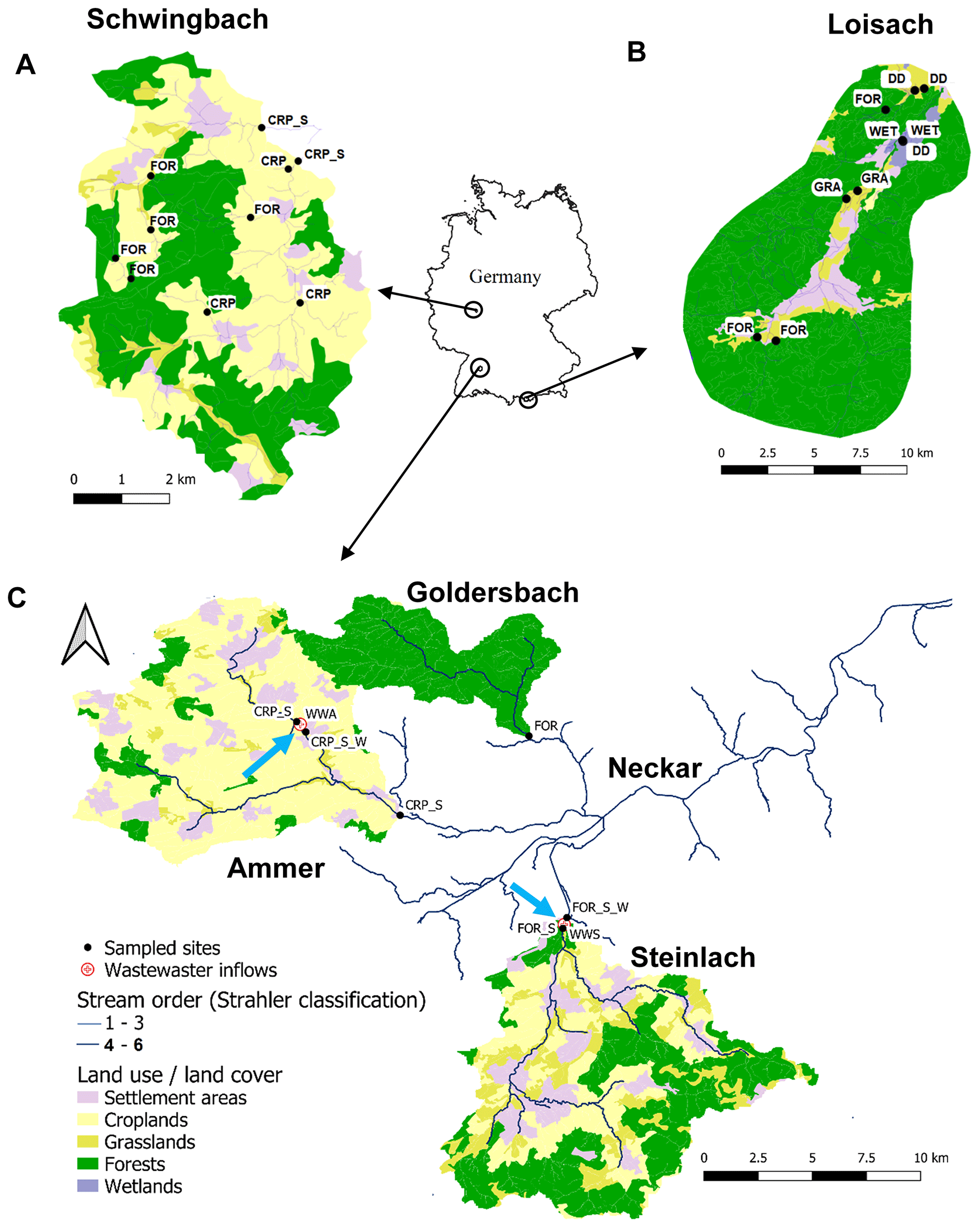
Figure 1Land cover maps of the (a) Schwingbach, (b) Loisach, and (c) Neckar sub-catchments (Goldersbach, Ammer, and Steinlach) derived from the CORINE Land Cover 2018 inventory with a 25 ha spatial resolution (https://land.copernicus.eu/pan-european/corine-land-cover/clc2018?tab=mapview). The black dots with labels (abbreviations explained in Table 1) represent sampled headwater streams and drainage ditch sampling points. Wastewater inflows sampled are indicated by blue arrows on the maps. Drainage ditches in the Loisach catchment were dug in the 1930s to 1960s in order to lower water levels to improve grassland productivity in areas formerly occupied by wetlands.
2.2 Sub-catchment delineation and land use classification
Sub-catchments for each sampling point in the Loisach, Goldersbach, Steinlach, Ammer, and Schwingbach catchments were delineated in QGIS (Quantum Geographic Information System) from a digital elevation model (DEM) (EU-DEM v1.1) with a 25 m resolution (European Copernicus mission, https://land.copernicus.eu/imagery-in-situ/eu-dem/eu-dem-v1.1, last access: 1 August 2021). Land use/land cover percentages of all the delineated sub-catchments were calculated from the CORINE Land Cover 2018 survey with a 25 ha spatial resolution (https://land.copernicus.eu/pan-european/corine-land-cover/clc2018?tab=mapview, last access: 1 August 2021). For data analysis, we classified sub-catchments according to their dominant land cover (> 50 % of the total area) into forest (FOR), cropland (CRP), grassland (GRA), and wetland (WET) and further differentiated sub-catchments with the influence of settlement areas (S) and wastewater inflows (W) (Table 1). As drainage ditches (DDs) in the Loisach catchment were added as an extra land use category, this classification resulted in nine land use classes (for details, see Table 1).
2.3 Hydrological and water physico-chemical characteristics
In the Loisach and Schwingbach catchments, discharge was calculated (Gore, 2007) from stream depth and velocity measurements using an electromagnetic sensor (OTT MF Pro, Hydromet, Germany). For streams in the Neckar sub-catchments, velocity was measured using the electromagnetic sensor (OTT MF Pro, Hydromet, Germany), and depth and discharge was obtained directly from gauging stations maintained by the water authority of the state of Baden-Württemberg (https://udo.lubw.baden-wuerttemberg.de/public/index.xhtml, last access: 1 August 2022). The slope of a ∼ 5 m reach at each sampling point was measured using a laser rangefinder with a slope function (Nikon Model: 8381, Japan). The slopes and velocities were used to model the site-specific gas transfer velocities (k in m d−1) for the quantification of daily GHG fluxes per unit stream surface area (mass m−2 d−1) (see details in the flux calculation section).
Discharge measurements at each sampling location and every sampling event were complemented by in situ measurements of water temperature (∘C), electrical conductivity (µS cm−1), dissolved oxygen (DO) (mg L−1), and pH using the ProDSS multiprobe (YSI Inc., USA). Water samples for nutrient and organic carbon analyses were also collected and filtered on-site through polyethersulfone (PES) filters (0.45 µm pore size, pre-leached with 60 mL of Milli-Q water). The samples were stored in 30 mL acid-washed high-density polyethylene (HDPE) sample bottles in triplicates and transported within 24 h to the laboratories at Karlsruhe Institute of Technology, Campus Alpin, Justus Liebig University Giessen, or the University of Tübingen. On arrival, all samples were immediately frozen for later analysis.
After unfreezing the samples overnight in a 4 ∘C refrigerator, the samples were directly analyzed for dissolved organic carbon (DOC), total dissolved nitrogen (TDN), nitrate (NO3-N), and ammonium (NH4-N) concentrations. Dissolved organic nitrogen (DON) concentrations were estimated as the difference between the TDN and dissolved inorganic nitrogen DIN (NO3-N + NH4-N) concentrations. DIN concentrations were determined using colorimetric methods, and the absorbance of the samples was measured using a microplate spectrophotometer (model: Epoch, BioTek Inc., USA). NO3-N concentrations were analyzed based on reactions with the Griess reagent (Patton and Kryskalla, 2011), and NH4-N concentrations were analyzed using the indophenol method (Bolleter et al., 1961). The DOC concentrations were measured as non-purgeable organic carbon (NPOC) using a TOC/TN analyzer (Analytik Jena, multi N/C 3100, Germany) after pre-treating the sample with 25 % HCl acid to remove the dissolved inorganic carbon (DIC). The TDN concentrations were analyzed simultaneously with the same instrument (Analytik Jena, multi N/C 3100, Germany).
2.4 Gas sampling, analysis, and calculations of annual areal fluxes
GHG stream, ditch, and wastewater samples were collected in triplicates simultaneously with the water physico-chemical samples using the headspace equilibration technique (Raymond et al., 1997). In brief, 80 mL of background water was equilibrated with 20 mL of atmospheric air in a syringe at in situ water temperatures. The headspace gas sample was transferred into 10 mL glass vials for GHG concentration analysis in the laboratory of the Karlsruhe Institute of Technology, Campus Alpin (see full sampling details in Mwanake et al., 2022). Atmospheric air samples were taken twice (morning and afternoon) on each sampling day to correct for background atmospheric GHG concentrations. GHG concentrations from the headspace were analyzed using a gas chromatograph (GC) (SRI 8610C, Germany) with an electron capture detector (ECD) for N2O and a flame ionization detector (FID) with an upstream methanizer for simultaneous measurements of CH4 and CO2 concentrations. The standards used for the GC calibration were 450, 800, 1000, 1500, 2000, and 3000 ppm for CO2; 1, 2, 3, 4, 5, and 6 ppm for CH4; and 0.4, 0.8, 1, 1.5, 2, and 3 ppm for N2O. Dissolved GHG concentrations in the stream water were calculated from post-equilibration gas concentrations in the headspace after correcting for atmospheric (ambient) GHG concentrations (e.g., Aho et al., 2019; Mwanake et al., 2022).
Daily diffusive fluxes (F) (mol m−2 d−1) of the GHGs were estimated using Fick's Law of gas diffusion, where F is the product of the gas exchange velocity (k) (m d−1) and the difference between the stream water (Caq) (mol m−3) and the ambient atmospheric gas concentration in water assuming equilibrium with the atmosphere (Csat) (mol m−3) (Eq. 1). GHG concentrations and fluxes were expressed in mass units by multiplying by the respective molar masses.
The temperature-specific gas transfer velocities (k) for each of the gases were calculated from normalized gas transfer velocities (k600) (m d−1) (corresponding to the k of CO2 at 20 ∘C with a Schmidt number of 600) and temperature-dependent Schmidt numbers (Sc) (unitless) of the respective gases (Eq. 2).
The k600 was modeled using Eq. (3) (drawn from Eq. 4 in Table 2 of Raymond et al., 2012), which was calibrated from headwater streams of similar characteristics as our study sites, where V is stream velocity (m s−1), and S is the slope (m m−1).
Before choosing the equation above for modeling the k600 values, we compared the k600 values calculated from all seven empirical models by Raymond et al. (2012). The predicted k600 values from models 3, 4, 5, and 6 in Table 2 of Raymond et al. (2012), which all use velocity and slope as input parameters, were mainly similar for the three discharge periods and across all stream orders 1–6 (ANOVA; p> 0.05). In contrast, the calculated k600 values from equations 1, 2, and 7, which use a stream depth parameter, were higher (ANOVA; p<0.05), particularly from the higher stream orders (5–6). This finding is inconsistent with the energy dissipation model of turbulent streams, where k600 is predicted to decrease with stream order. We, therefore, interpreted this to indicate a breakdown of these models for higher stream orders. This also agrees with Raymond et al. (2012) recommendations, and we, therefore, choose not to use models 1, 2, and 7 for this study. Out of the remaining Eqs. (3), (4), (5), and (6), we used Eq. (4), which calculated k600 based on the slope and velocity parameters and was also in line with several previous studies spanning a wide range of stream orders similar to our study (see Aho et al., 2019; Borges et al., 2019; Mwanake et al., 2019; Hall and Ulseth, 2020; Aho et al., 2021; Mwanake et al., 2022). The uncertainties in the modeled gas transfer velocities were reduced in this study by parametrizing the velocities and slopes based on actual field measurements of both variables. Equation (3) also estimated the gas transfer velocities in the drainage ditches with a measurable flow velocity and slope.
Water-to-atmosphere fluxes for all three GHGs across all land use classes in each sub-catchment were calculated from the mean daily CO2, CH4, and N2O fluxes during different discharge conditions. Total GHG fluxes were expressed as CO2 equivalent emissions (mg CO2 eq m−2 d−1) computed from global warming potentials (GWP100) using 28 for CH4 and 298 for N2O (IPCC, 2014). We followed the procedure developed in Mwanake et al. (2022) to scale tri-weekly measurements to annual flux estimates. Briefly, we classified each sampling date of every location into low, medium, or high discharge conditions according to whether normalized discharge fell in the 0 %–33 % (low), 34 %–66 % (medium), or 67 %–100 % (high) percentile days. Normalized discharge for each site was determined by dividing each absolute discharge measurement for every site visit during the year by the maximum measured discharge. The number of days in each discharge period was estimated as the ratio of observations in each discharge period to the total number of flux observations in individual land use classes in each catchment. CO2 equivalents fluxes were then calculated for the three different discharge periods in each land use class by multiplying the daily mean CO2 equivalents flux measured during each period and the number of days within each period. Annual fluxes were finally estimated by summing up the emissions of the low, medium, and high discharge periods for the individual land use classes in each catchment.
2.5 Statistical analysis
Linear mixed-effects models were used to investigate the effect of seasonality and land use on water physico-chemical variables, GHG concentrations, and fluxes (“lme4” package in R version 4.1.1). Fixed effects in the models consisted of land use classes in each catchment (Table 1) and season: summer 1 June–31 August, autumn 1 September–30 November, winter 1 December–28 February, and spring 1 March–31 May. Random effects accounting for repeated measures were also included in the models. Model performance was assessed based on the distribution of residuals (i.e., residuals should be normally distributed with a mean close to zero) and conditional r2 values calculated from significant models (p value < 0.05) (“MuMln” package in R). A Tukey post hoc test (p value < 0.05) of least-square means was used on the mixed models to identify individual differences within each categorical fixed effect. GHG concentration and flux data and other water physico-chemical variables were transformed using the natural logarithm to meet the assumption of normality. Because we quantified occasional negative fluxes in some of our sites, constant flux values of 50 mg m−2 d−1 for CO2-C, 0.5 mg m−2 d−1 for CH4-C, and 10 µg m−2 d−1 for N2O-N were added to the fluxes to enable the natural logarithm transformations.
Path analysis from structural equation models (SEMs, “lavaan” package in R version 4.1.1) was used to determine how environmental factors linked to seasonality and land use directly or indirectly influenced instream GHG production and consumption processes as well as external GHG sources, i.e., dissolved GHG inputs to the streams originating from either wastewater inflows or terrestrial landscapes which were not produced in situ. In brief, these SEMs were constructed based on causal relationships between environmental variables (interpreted as ultimate drivers of GHG concentrations) and substrate variables, which are affected by the environmental variables and also act as immediate drivers that affect GHG concentrations. Substrate variables in the models, which are known to influence in situ biogeochemical GHG production and consumption processes directly, included dissolved oxygen (DO) (% saturation), DOC (mg L−1), NH4-N (mg L−1), and NO3-N (mg L−1) concentrations (Battin et al., 2008; Stanley et al., 2016; Quick et al., 2019). The environmental variables in the models, which influence in situ GHG concentrations either directly by facilitating dissolved GHG inputs or indirectly by controlling the substrate variables, were water temperature (∘C) (a proxy for different seasons), stream velocity (V) (m s−1), percentage of upstream agricultural area for each sampling point (AGR: grassland + cropland area), and wastewater inflows (WW: Boolean numbers, i.e., 1 for the presence of wastewater inflow and 0 for absence).
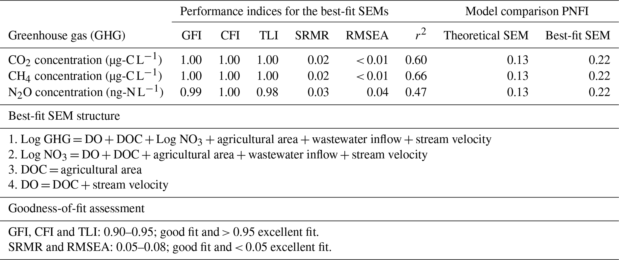
The hypothesized relationships between the substrate and environmental drivers of instream GHG concentrations were assessed in the overall theoretical SEM, which comprises several multivariate regression equations shown in Eqs. (4)–(8). To get the best-fit SEM, the removal of parts of the theoretical SEM was done manually until the model with the highest parsimony fit index (PNFI) and a root mean squared error of approximation (RMSEA) of < 0.05 was found (Schumacker and Lomax, 2015). Graphical representations of the significant relationship pathways from the best-fit model, including standardized slope parameter estimates, were done using the “semPlot” package in R software.
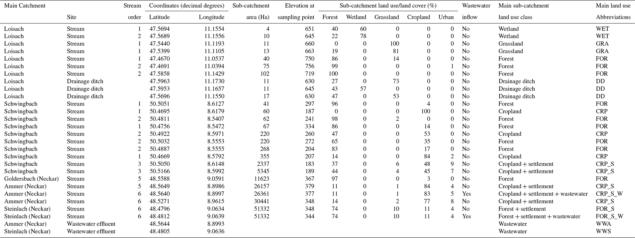
Table 1Summary descriptions of sampling sites located in the Schwingbach, Loisach, and Neckar sub-catchments (Goldersbach, Ammer, and Steinlach) (Fig. 1). The land use (%) was calculated for the site-specific upstream sub-catchments based on the CORINE Land Cover 2018 survey of Europe (see main text for details).
3.1 Hydrological variables
Across all sampling points and seasons, tri-weekly sampled stream velocity measurements (annual mean ± SE) were 2-fold higher for streams (0.19 ± 0.009 m s−1, range: 0.01–1.17) than ditches (0.05 ± 0.06 m s−1, range: 0.01–0.23) (Fig. A1). Seasonality had an overall significant effect (p value < 0.05) on stream velocities across all sampling points, with higher stream velocities observed in spring (0.24 ± 0.02 m s−1) than in autumn (0.12 ± 0.01 m s−1) (Tables 2, B2). Discharge in streams (3.9–18 500 L s−1) and in ditches (0.1–37 L s−1) was highly variable, reflecting differing stream sizes and seasonal variability (Fig. A1). The Neckar sub-catchments, dominated by streams (orders 5–6), had an order of magnitude higher mean annual discharge (874.7 ± 178 L s−1) than the streams in the other catchments (Loisach: 50.5 ± 6 L s−1, and Schwingbach: 26.7 ± 4 L s−1). The average discharge at the stream and ditch sampling points in all our study catchments were 3- to 5-fold higher in spring and summer (384.1 ± 96 and 526.4 ± 171 L s−1, respectively) than in autumn and winter (86.25 ± 13.07 and 157.3 ± 31.58, respectively; p value < 0.01; Tables 2, B2).
Table 2Results of multiple linear mixed-effects models predicting the effect of seasonality (summer, autumn, winter, and spring) and sub-catchment land use (Table 1) on stream velocity, discharge, water physico-chemical variables, GHG concentration, gas-transfer velocity, and GHG flux. The model performance was assessed based on conditional r2 and the distribution of residuals, including the variances explained by fixed effects and repeated measures' random effects.
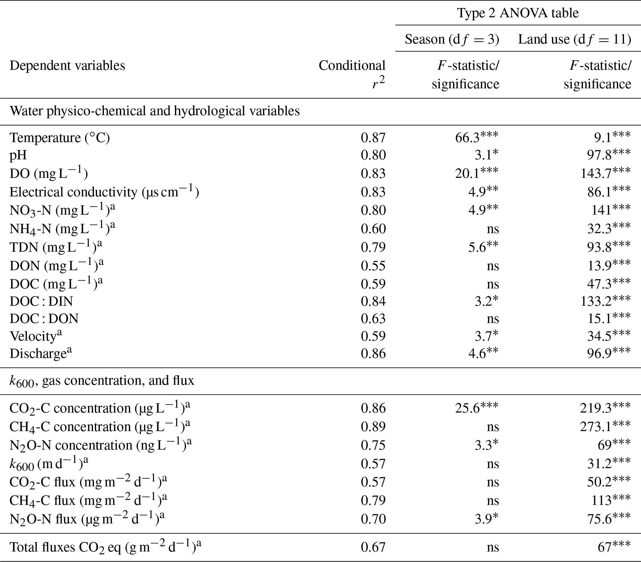
Level of significance (p value): * < 0.05, < 0.01, < 0.001, ns > 0.05. a Natural logarithm transformation. Conditional r2 is variance, explained by fixed and random effects of sampling date. df is degrees of freedom.
3.2 Water physico-chemical variables
3.2.1 Seasonal variation
Water temperature, DO, and pH ranged from 0.9–24 ∘C, 1.1–15.7 mg O2 L−1, and 6.7–9.0, respectively. Streams in the mountainous Loisach catchment had a mean annual (± SE) water temperature of 9.0 ± 0.2 ∘C, which was ∼ 1 ∘C colder than streams of the Schwingbach catchment (10.0 ± 0.4 ∘C) and 3∘ colder than streams in the Neckar sub-catchments (12.0 ± 0.3 ∘C). The annual ranges of NH4-N, NO3-N, DON, TDN, and DOC concentrations across all catchments were 0.05–1.0, 0.5–14.8, 0.05–10.9, 0.6–17.0, and 0.9–16.0 mg C L−1, respectively. DO, NO3, and TDN concentrations showed significant seasonal variability (Tables 2, B2). DO was higher in winter and spring than in summer and autumn (p value < 0.001). NO3-N and TDN concentrations were highest in winter and lowest in autumn and summer (p value < 0.01), while NH4-N, DOC, and DON showed no significant seasonal variation (p value > 0.05; Tables 2, B2). We additionally calculated DOC : DIN and DOC : DON molar ratios, which had interquartile ranges from 0.9–4.9 and 4.1–29.0, respectively. DOC : DIN ratios showed significant seasonal variability, with higher values in summer and spring than in winter (p value < 0.05), while no seasonal variability was found for DOC : DON ratios (p value > 0.05; Tables 2, B2).
3.2.2 Land use variation
Catchment land use was more significant than seasonality in explaining the variability of most water physico-chemical variables (p value < 0.001; Table 2). In the Loisach catchment, ditches had up to 2.6 times lower DO and 8 times lower NO3-N concentrations than the streams across all land use types (Fig. 2; Table B3). In contrast, NH4-N and DOC concentrations, as well as the DOC : DIN ratio, were 6–10 times higher in the ditches than in the streams (Fig. 2; Table B3). In the Neckar sub-catchments, forested streams had 1–2 times higher DO and DOC concentrations than cropland, settlement, and wastewater-influenced streams. The opposite was true for NO3-N and DON concentrations, which were an order of magnitude higher in the cropland-, settlement-, and wastewater-influenced streams than in the forested streams (Fig. 2; Table B3). As a result, DOC : DIN and DOC : DON ratios in the Neckar sub-catchments were, therefore, higher in forested streams than in cropland, settlement, and wastewater-influenced streams (Table B3).
In addition, cropland streams directly receiving wastewater inflows also had significantly lower DO and higher DOC than cropland streams without wastewater inflows (Fig. 2; Table B3). While NO3-N and DON concentrations were not significantly different in cropland streams with or without wastewater inflows, the concentrations of both variables were slightly higher in cropland streams with wastewater inflows (Table B3). In streams of the Schwingbach catchment, surrounding croplands and settlement areas also influenced NO3-N concentrations, which were up to 3-fold higher than in the forested streams. Across all the three catchments, DO concentrations, DOC : DIN ratios, and DOC : DON ratios were higher in the forested streams and decreased in streams of sub-catchments with predominant agricultural land uses or settlement areas, while the opposite was found for NO3-N and DON concentrations (Table B3). Additionally, forested streams in the Loisach catchment had an order of magnitude higher DOC : DON ratios than forested streams in the Neckar and Schwingbach catchments (Table B3).
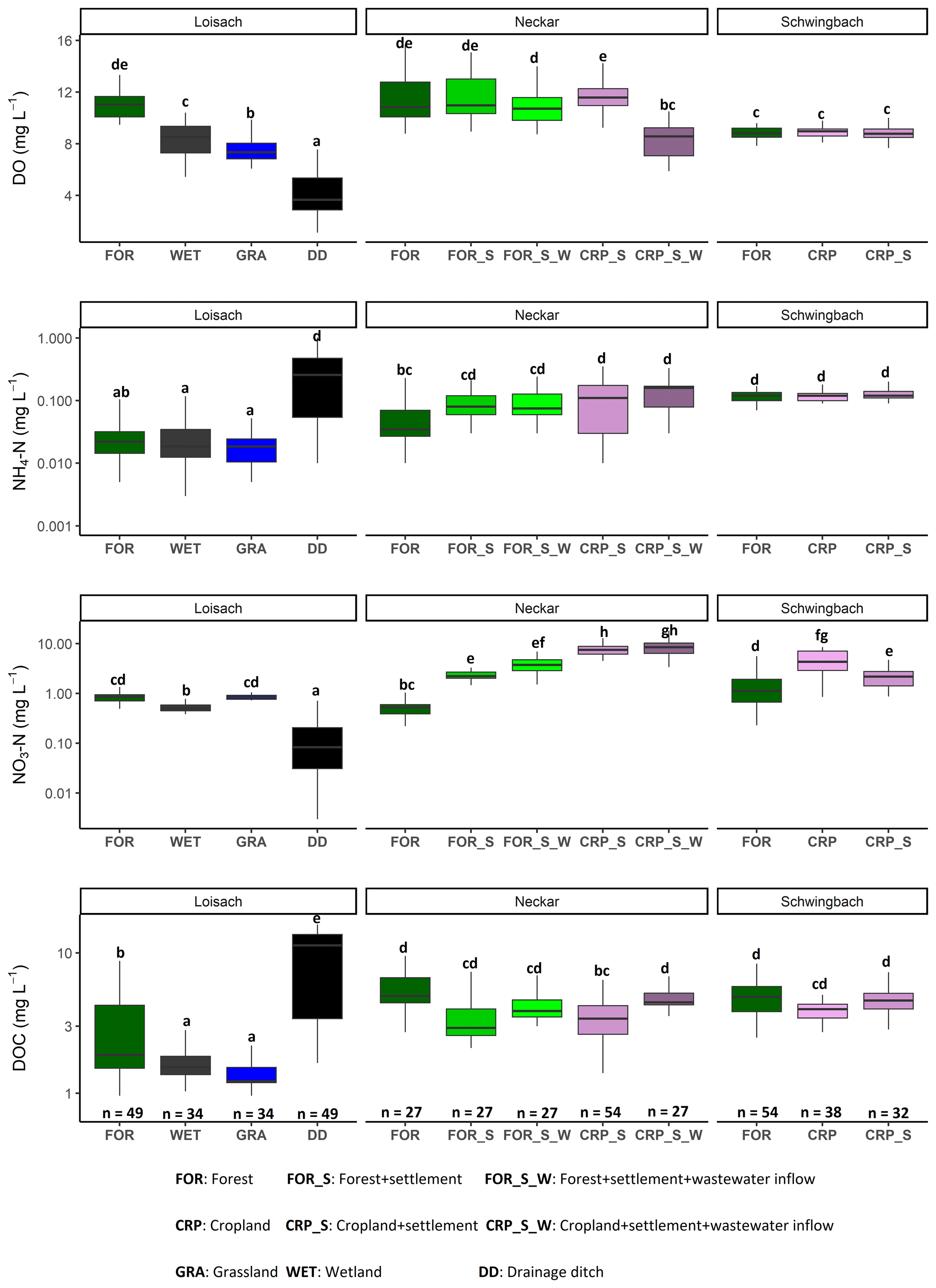
Figure 2Boxplots of DO, NH4-N, NO3-N, and DOC concentrations in stream and ditch waters in the three catchments grouped by dominating land uses (see Table 1 methods). The letters on top of the boxplots represent significant differences (p<0.05) among land use classes across the three catchments based on Tukey post hoc analyses from the linear mixed-effects model results (Table 2).
3.3 GHG concentrations and fluxes
3.3.1 Seasonal variation
In all headwater streams, CH4 and N2O concentrations varied greatly, spanning 3 orders of magnitude, i.e., from 0.03–58 µg-C L−1 (pCH4 1.3–2145 µatm) for CH4 and from 20–18 717 ng-N L−1 (pN2O 21–15 813 natm) for N2O. In contrast, CO2 concentrations varied less, spanning only 1 order of magnitude from 219–4868 µg-C L−1 (pCO2 369–7979 µatm). GHG concentrations in ditches also varied widely, with CH4, N2O, and CO2 concentrations spanning 1–2 orders of magnitude, ranging from 27–831 µg-C L−1 (pCH4 1469–34 482 µatm), 56–1540 ng-N L−1 (pN2O 35–1512 natm), and 1722–9746 µg-C L−1 (pCO2 2888–13 400 µatm), respectively (Figs. A2, A3).
Streams and drainage ditches across all seasons were predominantly sources of atmospheric CH4, N2O, and CO2, as indicated by concentrations mostly above the atmospheric background and the positive flux values displayed in Fig. 3. CO2 fluxes from streams ranged from −0.05–179 g C m−2 d−1 (mean 19 g C m−2 d−1), CH4 fluxes ranged from −0.40–325 mg C m−2 d−1 (mean 30 mg C m−2 d−1), and N2O fluxes ranged from −9.2–199.5 mg N m−2 d−1 (mean 12 mg N m−2 d−1). CO2 and CH4 fluxes from the ditches varied between 2–63 g C m−2 d−1 (mean 13.7 g C m−2 d−1) and from 117–7933 mg C m−2 d−1 (mean 1532 mg C m−2 d−1), respectively, while N2O fluxes ranged from −0.8–7.1 mg N m−2 d−1 (mean 1.2 mg N m−2 d−1).
Seasonal variations in GHG concentrations and fluxes were GHG-dependent and varied across the land uses within each catchment (Figs. 3, A2). In the Loisach catchment, there was a decline in instream CO2 concentrations in the summer, followed by a subsequent increase in autumn, particularly at non-forested sampling points (Fig. A2). Similar instream CO2 concentration trends, with lower values in the summer season and increasing values in autumn, were also found for non-forested streams of the Neckar sub-catchments (Fig. A2). However, non-forested streams of the Schwingbach catchments showed slightly different trends, with a decline in CO2 concentrations in spring and an increase in CO2 concentrations in the late summer (Fig. A2). Considering all data over all catchments, seasonality had an overall significant effect on CO2 (p value < 0.001), with summer concentrations being 1.6 times lower than in autumn, while CO2 fluxes showed no significant seasonal variability (p value> 0.05; Tables 2, B2).
In contrast to CO2, N2O concentrations in the Loisach and Schwingbach catchments decreased from summer to autumn but increased again towards the beginning of winter (Fig. A2). In autumn, N2O concentrations at first- and second-order forested streams in the Loisach and Schwingbach catchments were often below atmospheric concentrations (Fig. A2), characterizing these sites as N2O sinks (Fig. 3). A similar autumn decline in N2O concentrations was not observed in the streams of the Neckar sub-catchments, but rather, N2O concentrations increased from autumn to winter (Fig. A2). Across all catchments and sampling points, N2O concentrations were 2.4 times higher in winter than in the other seasons (p value < 0.05; Table B2). N2O fluxes were up to 1.6 times higher in summer and winter than in autumn and spring (p value < 0.05; Fig. 3; Table B2), which represented periods of either high N2O concentrations and moderate gas transfer velocities (winter) or moderate N2O concentrations and high gas transfer velocities (summer) (Table B2).
CH4 concentrations showed a seasonal pattern only in the Schwingbach catchment (Fig. A2), which showed a decline from summer through autumn and winter. This trend was not observed for the other catchments (Fig. A2) and resulted in a non-significant seasonal effect on both concentrations and fluxes when all data from all catchments were considered together (p value > 0.05; Tables 2, B2). Overall, GHG fluxes from streams within human-influenced land use classes (grasslands, croplands, and settlement areas) were more temporally variable (annual coefficient of variation > 55 %) than those in sub-catchments dominated by forests or wetlands (Fig. 3).
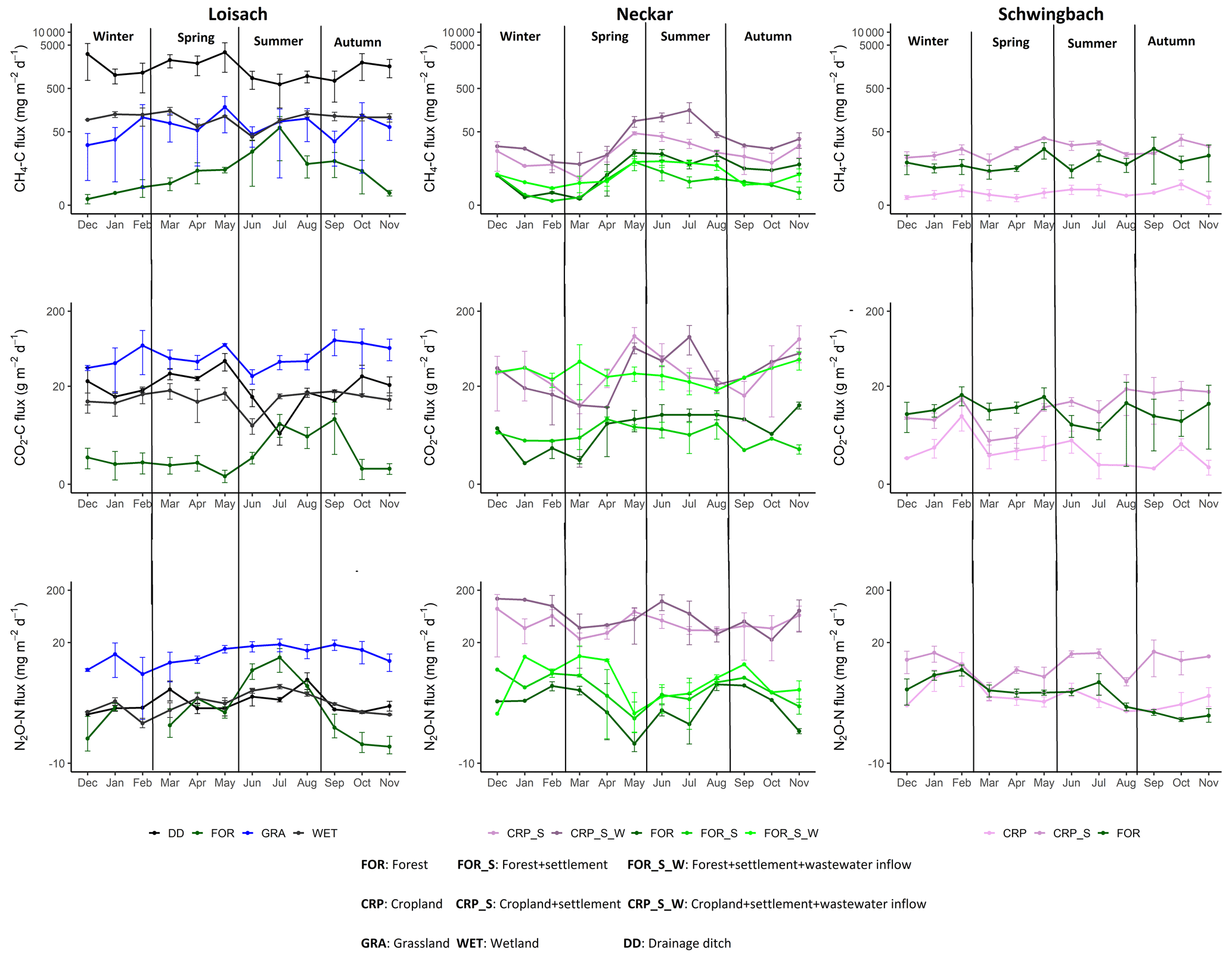
Figure 3Monthly mean ± SE of CO2, CH4, and N2O fluxes across all 26 sampled streams and ditches in the Loisach, Neckar, and Schwingbach catchments (see Table 1 methods). The colors of the lines and labels on the graph indicate the nine dominant land use classes.
3.3.2 Land use variation
Like water physico-chemical variables, the variability in GHG concentrations and fluxes was more strongly linked to catchment land use than seasonality (p value < 0.001; Table 2). In the Loisach catchment, CO2 concentrations and fluxes were an order of magnitude higher for the ditch and stream sites dominated by grassland land uses than forested-dominated sites (Figs. 3, 4; Table B3). N2O concentrations and fluxes in streams were also an order of magnitude higher in the grassland streams compared to the wetland and forested ones, with the latter functioning as occasional sinks for atmospheric N2O (Figs. 3, 4; Table B3). Wetland streams had higher CH4 fluxes than the other streams (Figs. 3, 4; Table B3). Overall, ditches showed up to 14 times more elevated CO2 and up to 850-fold higher CH4 concentrations than the streams of the Loisach catchment (Fig. A3; Table B3). In contrast, N2O concentrations in the ditches were highly variable, with higher and lower than atmospheric concentrations over the sampling year (Figs. A2, A3). CH4 fluxes were 2 orders of magnitude higher in ditches than in streams (Figs. 3, 4; Table B3). Interestingly, the ditches were even more often N2O sinks than forests, which resulted in the overall lowest N2O fluxes, e.g., 10 times lower than the ones of grassland-dominated streams (Fig. 3; Table B3)
In the Neckar sub-catchments, CO2, CH4, and N2O concentrations and fluxes were 1–10 times higher in the streams located in cropland and settlement areas compared to streams in forested areas (Figs. 3, 4, A3; Table B3). Generally, GHG concentrations and fluxes of streams in cropland and settlement areas further increased if wastewater inflows affected sampling points (Figs. 3, 4, A3; Table B3). For the latter, it is noteworthy that pronounced differences in wastewater characteristics existed in our study, even though the treatment procedures and the number of served households (80 000) were comparable for the two wastewater treatment plants. Overall, the wastewater outflow in the Ammer catchment had higher TDN, DOC, CH4, and N2O concentrations than the Steinlach catchment (Table B1). In contrast to the other two catchments, forested streams in the Schwingbach catchment had CO2 and CH4 concentrations and fluxes comparable to cropland- and settlement-influenced streams within the catchment (Figs. 3, 4, A3; Table B3). However, N2O concentrations and fluxes were higher in streams with cropland and settlement influences than in forested streams (Figs. 3, 4, A3; Table B3).
In addition to land use effects, we also examined spatial variability in the GHG concentrations and fluxes linked to stream order differences. We found tendencies of higher CO2, CH4, and N2O concentrations and fluxes with increasing stream orders in the Schwingbach and Neckar catchments dominated by croplands and settlement areas. In contrast to the Neckar and Schwingbach catchments, GHG concentrations and fluxes in the more natural Loisach catchment decreased with stream order (Fig. A4). Comparing across catchments, higher stream orders (5 and 6) in the human-influenced Neckar catchment had higher or comparable GHG concentrations and fluxes than lower stream orders (1–3) in the Schwingbach and Loisach catchments (Fig. A4).
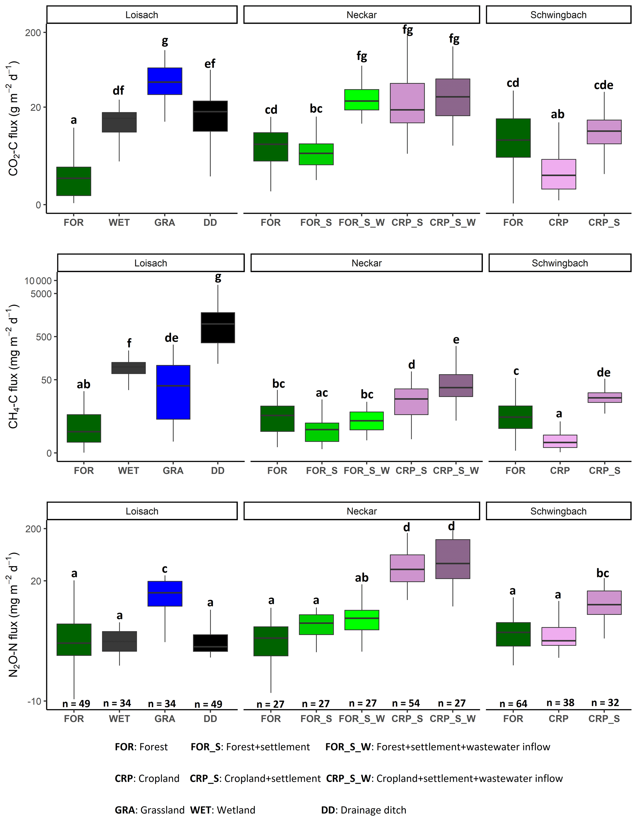
Figure 4Boxplots of CO2, CH4, and N2O fluxes in stream and ditch waters in the three catchments grouped by land uses (see Table 1 methods). Letters on top of the boxplots represent significant differences (p<0.05) amongst the land use classes across the three catchments based on Tukey post hoc analyses from the linear mixed-effects model results (Table 2).
3.4 Direct and indirect drivers of greenhouse gas concentrations
We used path analyses from best-fit SEMs based on all our datasets to explain how environmental factors such as upstream agricultural area, wastewater inflow, and stream velocity controlled the spatial-temporal dynamics of GHG concentrations that drove the fluxes. The slope parameter estimates from the SEMs revealed significant (p value < 0.05) interactions between the environmental variables and DO (% saturation), DOC mg L−1, and NO3-N mg L−1, i.e., substrate variables that directly control in situ GHG concentrations (Fig. 5, Table B4). In contrast to all other variables, water temperature and NH4-N mg L−1 did not contribute significantly (p value > 0.05) to the variance explained by the best-fit SEMs and were removed from the final path analyses (Table B4). That said, an increase in the upstream agricultural area resulted in a ∼ 46 % increase in in situ NO3-N concentrations. Wastewater inputs resulted in a ∼ 23 % increase in in situ NO3 concentrations, while DOC concentrations were not significantly affected. DO decreased with increasing DOC concentrations, while NO3-N concentrations followed an opposite pattern and increased with increasing DO concentrations (Fig. 5).
CO2 and CH4 concentrations had a negative relationship with DO (Fig. 5a–b), but N2O concentrations were not significantly related to DO (Fig. 5c). Besides DO, CO2 concentrations decreased by 17 % with stream velocity, increased by 18 % with wastewater inflows, and increased by 23 % with upstream agricultural area (Fig. 5a). CH4 concentrations also decreased by 16 % with increasing stream velocity. However, the effect of the increased share of agricultural areas (+11 %) on CH4 concentrations was lower than for CO2. Additionally, CH4 concentrations also decreased by 29 % with increasing NO3-N concentrations (Fig. 5b). In contrast to CO2 and CH4, N2O concentrations increased by 43 % with increasing NO3-N concentrations, while the effect of stream velocity was of minor importance (−8 %). Compared to CH4 and CO2, N2O concentrations in stream and river waters showed similar or stronger relationships to wastewater inflows (+16 %) and upstream agricultural area (+32 %) (Fig. 5c). Overall, the best-fit SEMs explained 60 %, 66 %, and 47 % of the observed variances in CO2, CH4, and N2O concentrations, respectively (Table B4).
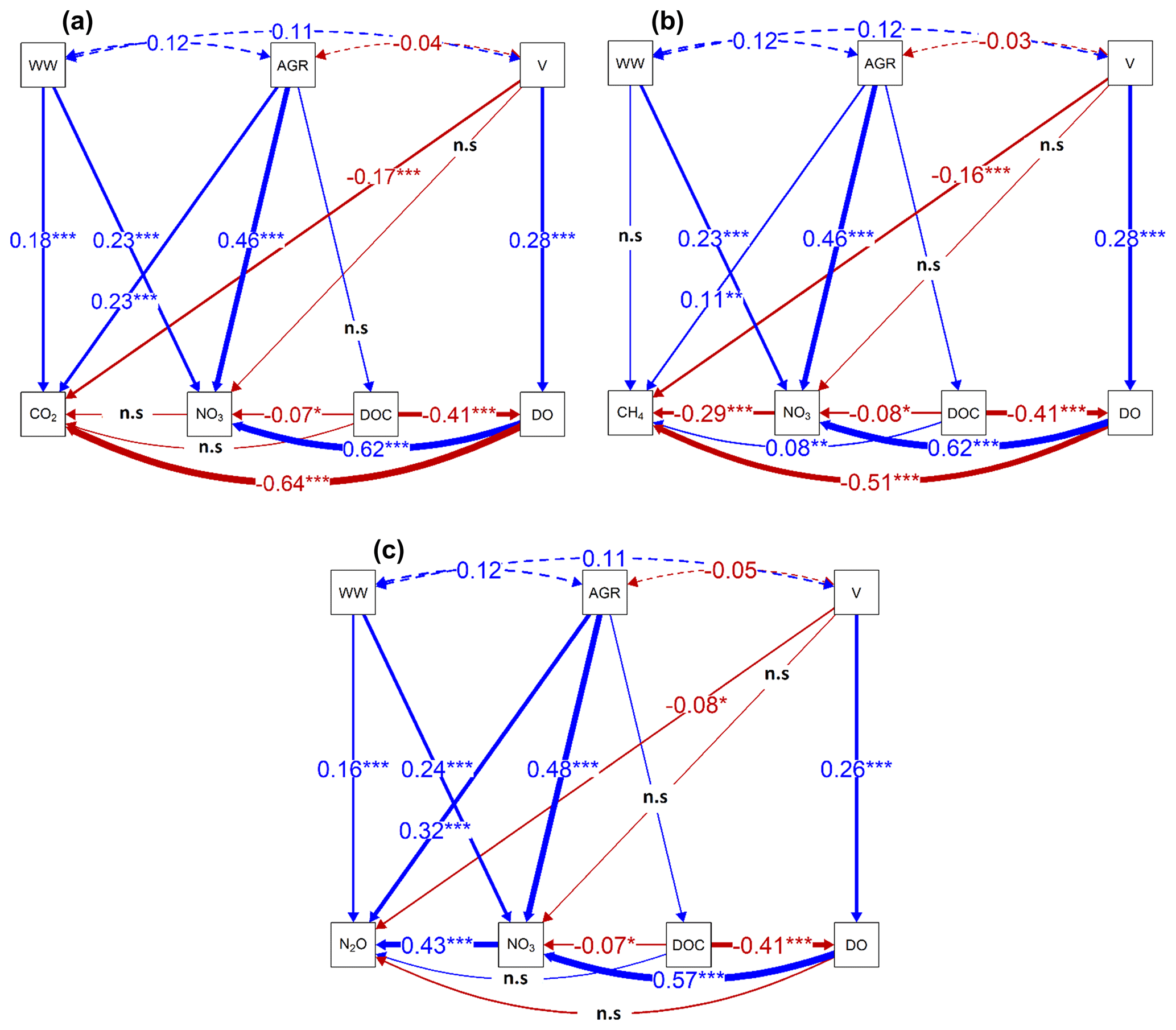
Figure 5Regression pathways predicting (a) Loge CO2 concentration µg-C L−1, (b) Loge CH4 concentration µg-C L−1, and (c) Loge N2O concentration ng-N L−1 across all sampling points and seasons from best-fit SEMs consisting of substrate (DO, DOC, and NO3-N) and environmental variables (stream velocity (V)), percentage agricultural area (AGR; grassland + cropland areas), and wastewater inflows (WW). The numbers on the lines represent standardized slope parameters, with significant (p value < 0.05) relationships indicated by * and non-significant (p value > 0.05) relationships indicated by ns. Solid lines represent fitted relationships, while dashed lines represent co-variances in the environmental variables. Blue lines represent positive relationships, and red represents negative relationships, with width representing the strength of the relationships.
3.5 Annual areal fluxes
Based on global warming potential calculations, CO2 dominated the annual GHG emissions across all headwater catchments, with contributions ranging from 57 %–100 %. The non-CO2 gas contributions were much lower and ranged from 0 %–43 % for CH4 and 0 %–18 % for N2O (Fig. 6). The highest contribution of CH4 (43 %) was found at ditch sampling points in the Loisach, while the highest N2O contributions (up to 18 %) were observed at the cropland-influenced streams fed by wastewater inflows in the Neckar sub-catchments (Fig. 6). Overall, the annual CO2 equivalent emissions from anthropogenic-influenced streams (∼ 71 kg CO2 m−2 yr−1) were up to 20 times higher than from natural forested streams (∼ 3 kg CO2 m−2 yr−1; Fig. 6). Its also noteworthy that the total annual GHG emission from oligotrophic forested streams in the Loisach catchment was significantly lower than other forested catchments in the more human-influenced Schwingbach and Neckar sub-catchments (Fig. 6).
Regarding different discharge periods, high and medium discharge periods contributed up to 91 % to total GHG emissions in anthropogenic-influenced streams but only 4 % in forested streams (Fig. 6). Overall, the high and medium discharge periods contributed the most to the annual fluxes quantified in lower-order streams (Strahler 1–2) and ditch sampling points, which were prevalent in the Loisach and Schwingbach sub-catchments (Figs. 6b, c). The opposite was true for larger forested and cropland streams in the Neckar sub-catchment, where higher annual flux contributions occurred primarily in the low discharge period (Fig. 6a). However, this pattern did not hold for cropland streams with the wastewater inflows in the same catchment, with the sites showing an 82 % increase in annual emissions during the high and medium discharge periods (Figs. 6b, c).
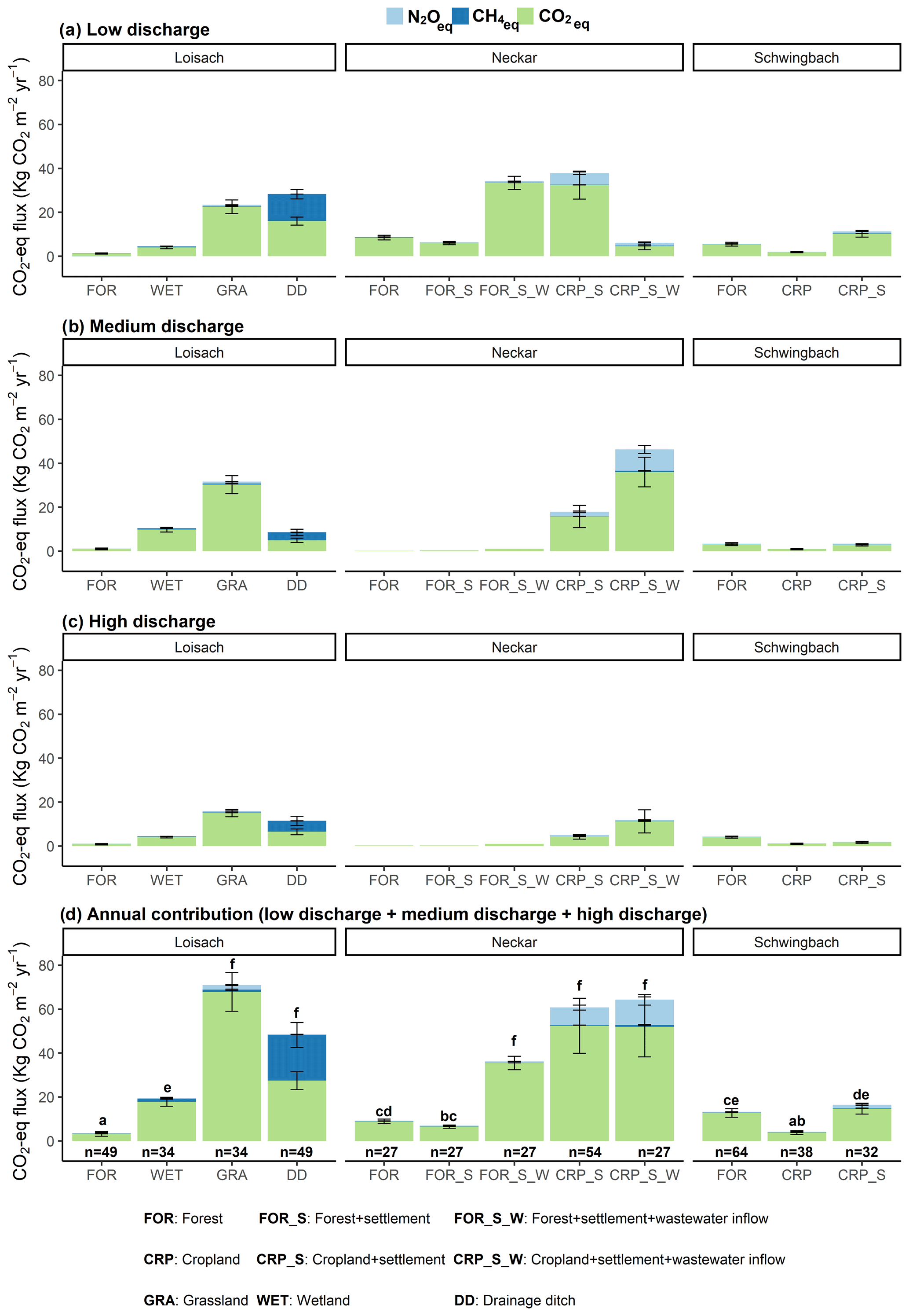
Figure 6Areal CO2 equivalent fluxes (mean ± SE) grouped by GHG type for each land use class during (a) low, (b) medium, and (c) high discharge periods. Panel (d) represents the total annual fluxes by summing up contributions from the three discharge periods. Letters on the bar graphs represent significant differences (p<0.05) in the annual areal emissions amongst the land use classes across the three catchments based on Tukey post hoc analyses from the linear mixed-effects model results (Table 2).
The GHG fluxes quantified from headwater streams and ditches in this study add to the growing evidence that both aquatic ecosystems are significant net emitters of GHGs to the atmosphere. In agreement with previous studies, CO2 accounted for most (> 81 %) of the annual fluvial GHG fluxes in CO2 equivalents (e.g., Marescaux et al., 2018; Mwanake et al., 2022; Li et al., 2021). However, the presence of upstream agricultural and settlement areas seemed to alter these trends by reducing the contribution of CO2 and increasing N2O and CH4 contributions. The effects of the above anthropogenic activities on aquatic GHG dynamics were twofold. Drainage ditches were landscape hotspots for CH4 emissions, while increasing upstream agricultural and settlement areas resulted in fluvial N2O hotspots. The emissions from human-influenced streams were further supplemented by wastewater inflows, which provided year-long nutrients, labile carbon, and GHG supplies, resulting in much higher CO2 and N2O annual emissions. Besides influencing GHG hotspots, the temporal dynamics of GHG fluxes from streams and ditches in our study were further impacted by anthropogenic influences. While catchments dominated by wetlands or forested areas exhibited low seasonal variabilities due to limitations in conditions that favor peak emissions (increased gas transfer velocities and sufficient GHG supplies), opposite trends were found at catchments dominated by agricultural and settlement areas or affected by wastewater inflow. These findings suggested that the occasional peak GHG emissions in the later catchments represented periods where external GHG sources from supersaturated terrestrial soils or wastewater inflows outweighed supply constraints during peak discharge periods with high gas transfer velocities. These findings suggest that future land use changes from natural forests to agricultural and settlement areas may increase the radiative forcing of aquatic GHG emissions by increasing the magnitudes of their annual fluxes, especially in a changing climate with more extreme discharge conditions.
4.1 Seasonal variability in GHG concentrations and fluxes
Seasonal trends in in situ GHG concentrations and fluxes were mainly linked to substrate availability (C and N), discharge, and temperature, similar to previous studies on other streams in temperate climates (Dinsmore et al., 2013; Deirmendjian et al., 2019; Herreid et al., 2021). The low in situ CO2 concentrations (< 100 % saturation) during summer (Table B2) suggested elevated photosynthetic uptake within the streams and ditches, which is in line with the results of a recent meta-analysis on lotic ecosystems (Gómez-Gener et al., 2021). The decline in CO2 concentrations in summer was most apparent at the non-forested stream sampling points, with higher canopy cover in the forested areas likely limiting in situ stream photosynthesis due to shading effects. These non-forested sites also had higher instream dissolved inorganic nitrogen concentrations, nutrient conditions previously shown to favor macrophyte photosynthetic uptake of CO2, resulting in lower in situ stream CO2 concentrations (Deirmendjian et al., 2019). We also found that stream and ditch waters were oversaturated with CO2 in autumn and winter. These seasons are characterized on the one hand by low discharge and low stream velocity, conditions which likely reduce degassing rates, and on the other hand by elevated in situ C metabolism, as supported by low DO concentration in autumn, which indicates respiratory O2 consumption (e.g., Borges et al., 2018). We attribute the lack of seasonality in CO2 fluxes (Table B2) to the compensatory effects of seasonally varying stream velocities and CO2 source strengths. For example, high CO2 concentrations and low gas transfer velocities in autumn and vice versa in spring resulted in comparable CO2 fluxes in the two seasons (Table B2).
N2O concentrations also varied significantly across seasons, but the pattern differed from that of CO2. In autumn, forested lower-order streams in the Loisach and Schwingbach catchments mainly showed N2O concentrations below atmospheric background concentrations and were temporary sinks of N2O (Fig. 3). This finding could be related to increased inputs of organic matter in these headwater catchments due to leaf fall, providing additional organic carbon for microbial metabolism in this period, which likely increased the demand for terminal electron acceptors such as O2, NO3, and N2O. This conclusion is also supported by the lowest DO and NO3-N concentrations during autumn, which could suggest the dominance of complete denitrification in the streams (Quick et al., 2019). With decreasing temperatures towards winter, lower productivity and N demand within the streams resulted in the accumulation of NO3-N, which seemed to favor internal N2O production, as seen by the positive relationship between the two variables (Fig. 5c). The high sensitivity of the N2O reductase to low temperatures might have further supported elevated N2O concentration and fluxes during winter (e.g., Holtan-Hartwig et al., 2002). A similar finding of high winter N2O concentrations and fluxes was also found in other temperate streams, alluding to similar controls of temperature and nutrient availability (Herreid et al., 2021; Galantini et al., 2021). Thus, based on our results, winter periods can significantly contribute to annual N2O emission budgets. Yet, to the best of our knowledge, temperate studies covering the winter period are still scarce. In contrast to CO2 and N2O, neither CH4 concentrations nor fluxes showed any seasonal trends. Such a finding is similar to what was found in a global meta-analysis (Stanley et al., 2016), where multiple controls related to substrate availability, geomorphology, and hydrology were shown to result in a high spatial-temporal variance of CH4, thus masking any seasonal emission patterns.
4.2 Effect of human impacts on GHG concentrations and fluxes
Anthropogenic-influenced streams and ditches draining predominantly agricultural and settlement areas showed higher CO2 equivalent GHG emissions than forested streams (Fig. 6). Such a finding is similar to other studies in the temperate region (e.g., Borges et al., 2018; Deirmendjian et al., 2019; Galantini et al., 2021). The high GHG emissions of streams and ditches in agricultural and settlement areas are likely due to elevated hydrological inflow (e.g., via groundwater and interflow) of nitrogen and labile carbon (e.g., Lambert et al., 2017; Deirmendjian et al., 2019; Mwanake et al., 2019) or terrestrially originating dissolved GHGs linked to lower vegetation cover compared to forested catchments (e.g., Deirmendjian et al., 2019; Mwanake et al., 2022). This interpretation could be supported by the significant positive relationships that we found between percentage agriculture and stream CO2, CH4, and N2O, as well as nitrate concentration and a positive trend for DOC (Fig. 5).
Low DOC : DON ratios have previously been linked to more labile and less aromatic forms of dissolved organic matter (DOM) (Sebestyen et al., 2008; O'Donnell et al., 2010). We found significantly lower DOC : DON ratios in streams and ditches in agricultural and settlement areas than in forested streams, suggesting that the more bioavailable DOM in the human-influenced ecosystems favored elevated GHG production through heterotrophic processes (e.g., Bodmer et al., 2016). Such differences in DOC : DON ratios were also found amongst forested streams, with a decreasing trend from the Loisach, Neckar, to Schwingbach catchments, which may also explain the differences in their GHG emissions (Fig. 6). The differences in the DOM bioavailability of forested streams in the three catchments may suggest differences in DOM flow paths during terrestrial–groundwater–stream interactions. We contend that the moderately sloping streams of the Neckar and Schwingbach catchments likely had lower DOC : DON ratios due to longer water residence times and higher contributions of groundwater inflow (e.g., Sebestyen et al., 2008) than those in the steeper forested catchments of the Loisach (Table B3). The distinct difference in water stable isotope signatures, i.e., the shift of precipitation vs. stream water seasonality across the three catchments (Mwanake et al., 2023), further supported the difference in water residence times and their relationships with stream slope (e.g., Zhou et al., 2021).
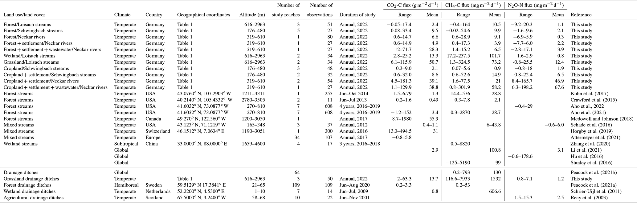
Table 3Compilation of GHG emissions from temperate streams and ditches mostly with comparable land use, climate, and altitude ranges.
In addition to land use influences, wastewater inflows into streams in agricultural and settlement areas further increased GHG concentrations and fluxes. The two sampled wastewater effluents, which drained into the Steinlach and Ammer streams of the Neckar sub-catchments, showed higher GHG concentrations than the stream water upstream of the inflows (Fig. A5, Table B1), which mainly led to increased GHG concentration and fluxes also downstream of the wastewater inflows. This finding is similar to what was found in other temperate studies comparing stream GHG concentration upstream and downstream of wastewater inflows (e.g., Marescaux et al., 2018; Aho et al., 2022). However, due to higher background GHG fluxes in the cropland than in the forested sub-catchments (Fig. 4), differences in the total GHG emissions before and after wastewater inflow were more pronounced in the forested sub-catchments (Fig. 6). In addition to the pronounced differences in the quality of the wastewater effluent (Table B1), this finding also shows the importance of background GHG fluxes as influenced by catchment land use in assessing how wastewater inflows affect riverine GHG emissions.
Apart from land use influences, GHG fluxes from streams have previously been shown to decrease with stream order, as dissolved GHG inputs from groundwater and terrestrial sources also reduce (e.g., Hotchkiss et al., 2015; Turner et al., 2015; Mwanake et al., 2022). While our study design was not meant to explicitly assess stream order influences due to limited replication across a wide range of stream orders, we did find an opposite trend with stream order, similar to other studies in anthropogenic-influenced catchments (e.g., Borges et al., 2018; Marescaux et al., 2018). For example, higher-order streams (stream orders > 5) in the Neckar sub-catchments dominated by croplands and with wastewater influences had either higher or comparable GHG fluxes than lower-order streams (stream orders < 3) in the Loisach and Schwingbach catchments. We, therefore, show a potential breakdown of stream order–GHG relationships in highly human-impacted lotic ecosystems, with disproportionately higher GHG emissions than in more natural ecosystems. We also show that significant nutrient and labile carbon supplies to higher-order streams, which create ideal conditions for GHG production and emission, may outweigh the physical disadvantages (e.g., lower surface area to volume ratio) of higher-order streams relative to lower-order streams.
Drainage ditches, characterized by low flow velocities and high DOC : DIN ratios, functioned as strong sources of CO2 and CH4 fluxes compared to streams. In addition to draining CO2- and CH4-rich wetland and grassland soils, we assume that the low DO, high DOC, and low NO3-N concentrations, along with high water retention times, supported high in situ CH4 production rates in the ditch sediments, resulting in their overall highest contribution of CH4 fluxes to total annual GHG emission budgets than streams (Fig. 6). This interpretation is further supported by a significant negative relationship between CH4 and DO, as well as NO3-N concentrations, and a positive relationship with DOC concentrations, associations which have also previously been linked to in situ methane production in fluvial ecosystems (e.g., Baulch et al., 2011a; Schade et al., 2016). High CH4 fluxes from drainage ditches were also found in other studies from both forested and wetland areas (e.g., Schrier-Uijl et al., 2011; Peacock et al., 2021a). Contrastingly, ditches were only weak sources or even sinks for atmospheric N2O. This finding suggests N2O reduction to N2 via complete denitrification, an interpretation already made in previous studies on lotic ecosystems (e.g., Baulch et al., 2011b; Mwanake et al., 2019).
4.3 Comparison of GHG flux magnitudes with regional and global studies
This study's daily CH4 and N2O diffusive flux ranges from both streams and ditches are mostly within the same order of magnitude as those previously reported in global synthesis studies (Table 3: Hu et al., 2016; Stanley et al., 2016). In contrast, this study reported among the highest fluvial CO2 emissions compared to other regional and global studies, with significant mean fluxes of up to 51 g C m−2 d−1 (Table 3). We attribute this finding to moderate–steep slopes such as those quantified in the mountain streams of the Loisach catchment or diffuse and point terrestrial dissolved CO2 inputs from the more human-influenced Schwingbach and Neckar catchments, translating to higher fluvial CO2 fluxes (Fig. 6). However, our high CO2 fluxes are comparable with those quantified from other temperate streams in Canada and Switzerland with similar moderate–steep slopes and considerable dissolved CO2 inputs from terrestrial landscapes (e.g., Mcdowell and Johnson. 2018; Horgby et al., 2019). The CH4 fluxes from streams in this study are comparable with those previously found in temperate sub-catchments with similar land uses and altitudes but are lower than those reported from permafrost streams in China (Table 3; Zhang et al., 2020). Our N2O fluxes from cropland-, settlement-, and wastewater-influenced streams are higher than those previously reported in a mixed land use catchment (Schade et al., 2016). Still, our forest N2O fluxes are in the same range as those of other temperate forested streams (Aho et al., 2022). That said, these comparisons may be hampered, particularly for fluvial N2O fluxes, by the limited number of available studies (Table 3).
The average ditch CH4 fluxes in this study are higher than those reported for forest and wetland draining ditches in boreal and temperate regions (Table 3: Schrier-Uijl et al., 2011; Peacock et al., 2021a) and the global mean provided by Peacock et al. (2021b), which includes estimates from large canals. In contrast, N2O fluxes from ditches in this study are lower than those quantified from NO3-N-rich agricultural ditches in temperate regions (Table 3: Reay et al., 2003).
Streams and ditches in agricultural and settlement areas were characterized by significantly higher GHG fluxes with more significant intra-annual variabilities than forests and wetlands. A combination of wastewater inflows and agricultural land use resulted in the highest fluvial CO2, CH4, and N2O fluxes, particularly during high discharge periods with substantial external dissolved GHGs. In general, anthropogenic activities resulted in a potential breakdown of the expected decrease of the GHG source strengths with increasing stream order, as higher-order streams in the Neckar sub-catchments with cropland and settlement influences had either higher or comparable concentrations and fluxes than small streams in the Loisach and Schwingbach catchments. As most studies use stream order to upscale local and regional riverine fluxes, we show from our results that caution must be taken in applying the methodology, particularly across catchments differing in land use intensity.
Our findings indicate that future work should focus more on human-influenced headwater stream ecosystems, as they contribute disproportionately large annual fluxes and are more temporally variable than natural ones. Our study also found higher winter N2O fluxes, emphasizing the need for continuous sampling regimes covering full years to reduce uncertainty in annual GHG emission estimates. Combining continuous sampling regimes of all three biogenic GHGs (CO2, N2O, and CH4) across catchments with contrasting land uses will further constrict riverine emissions and aid in developing targeted emission reduction mitigation strategies.
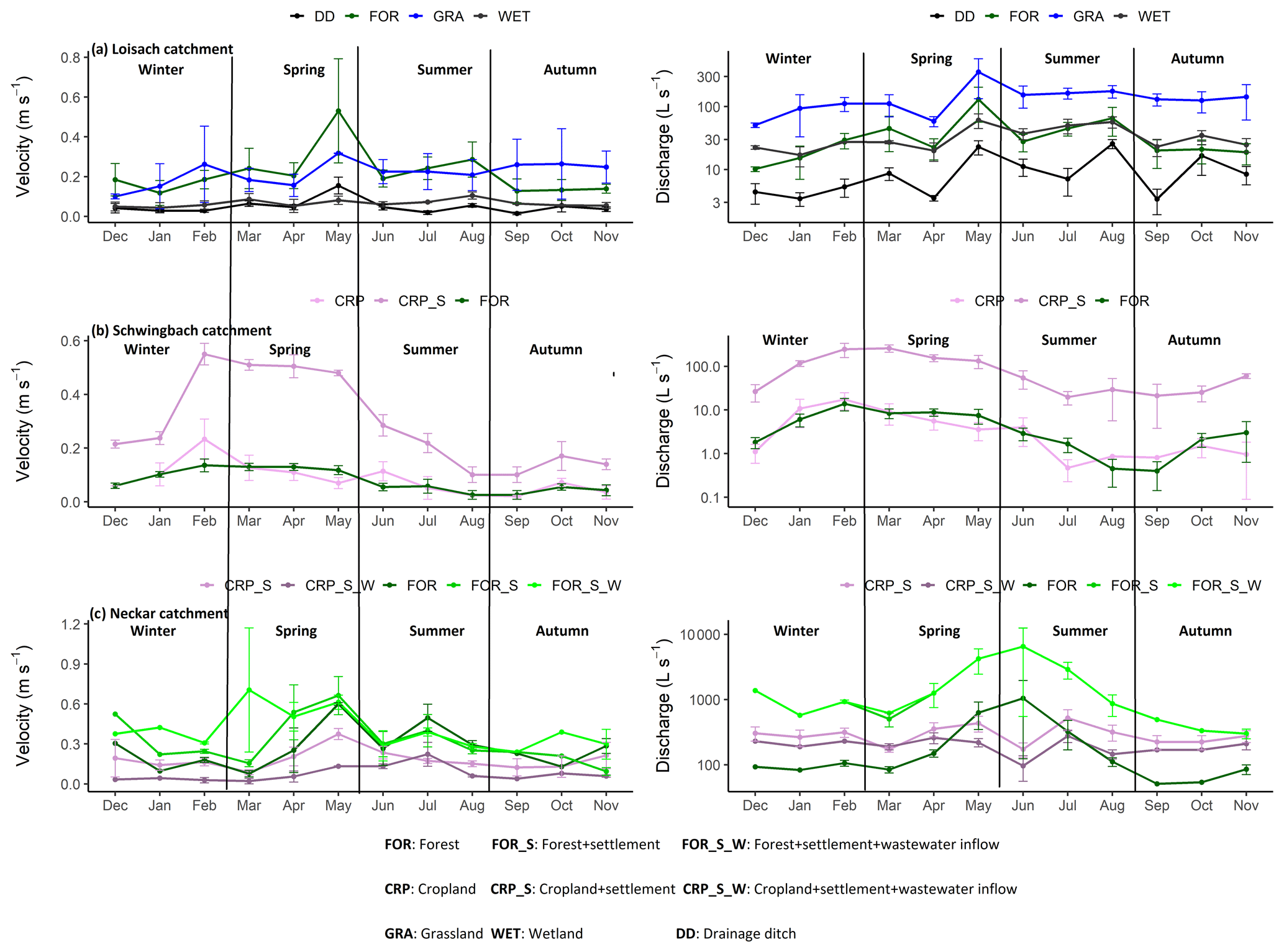
Figure A1Monthly mean ± SE velocity and discharge grouped by land use/land cover classes in the (a) Loisach, (b) Schwingbach, and (c) Neckar catchments.
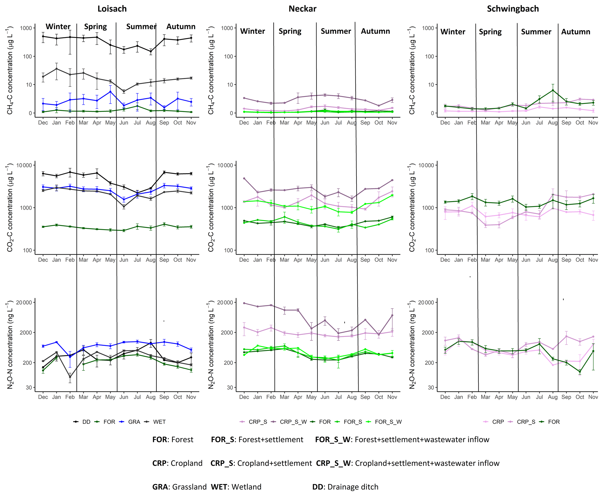
Figure A2Monthly mean ± SE CO2, CH4, and N2O concentrations at sites within the Loisach, Neckar, and Schwingbach catchments.
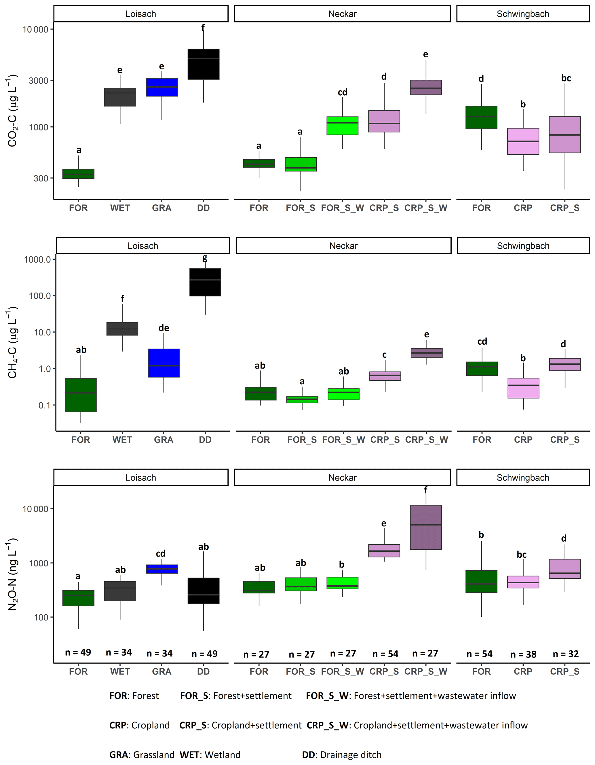
Figure A3Boxplots of CO2, CH4, and N2O concentrations in stream and ditch waters in the three catchments grouped by dominating land uses (see Table 1 methods). The letters on top of the boxplots represent significant differences (p<0.05) amongst the land use classes across the three catchments based on Tukey post hoc analyses from the linear mixed-effects model results (Table 2).
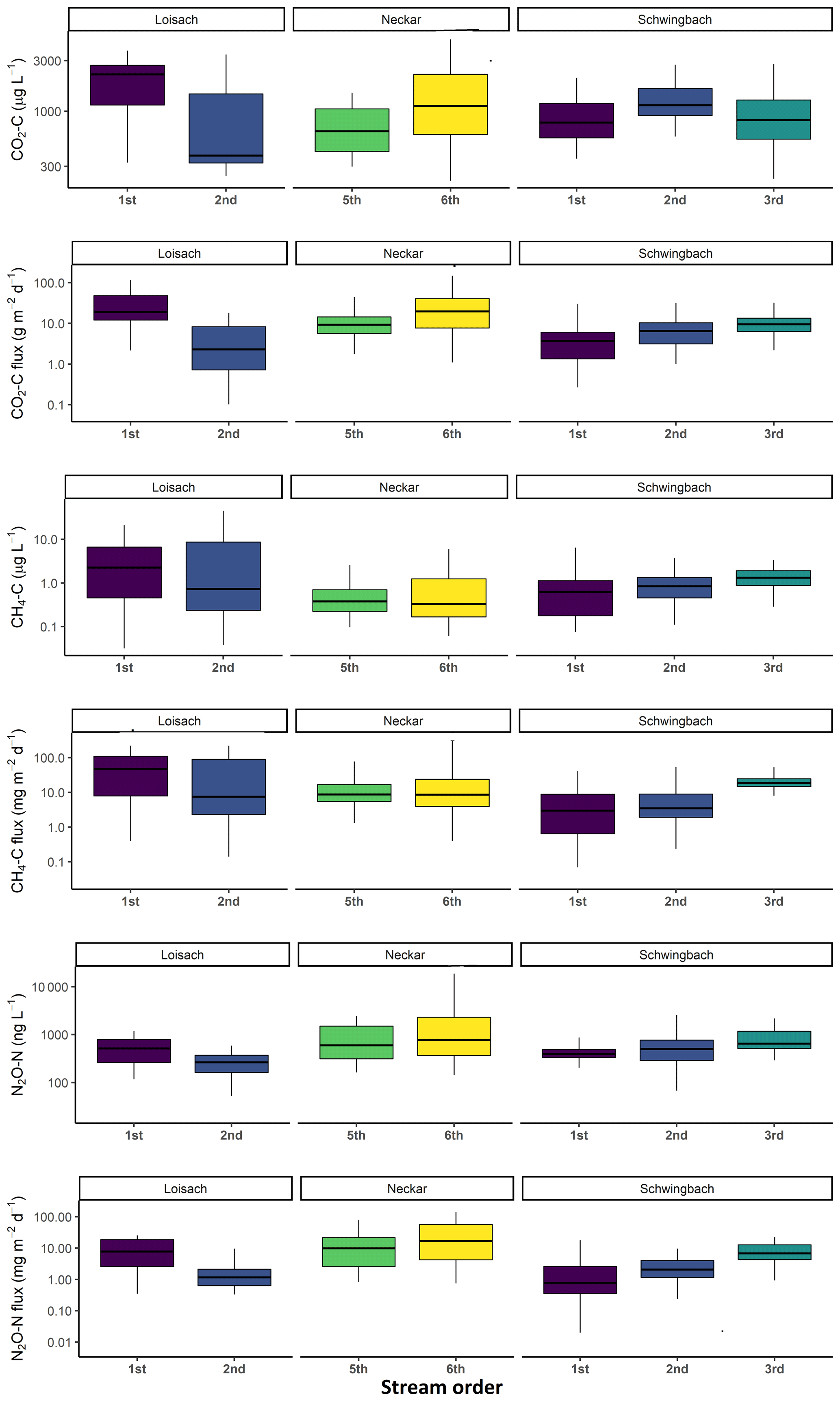
Figure A4Boxplots of stream CO2, CH4, and N2O concentrations and fluxes in the three catchments grouped by stream order (see Table 1 methods).
Table B1Annual means (+ SE) of water chemistry variables and gas concentration measured in the effluents of the Ammer (WWA) and Steinlach (WWS) wastewater treatment plants.
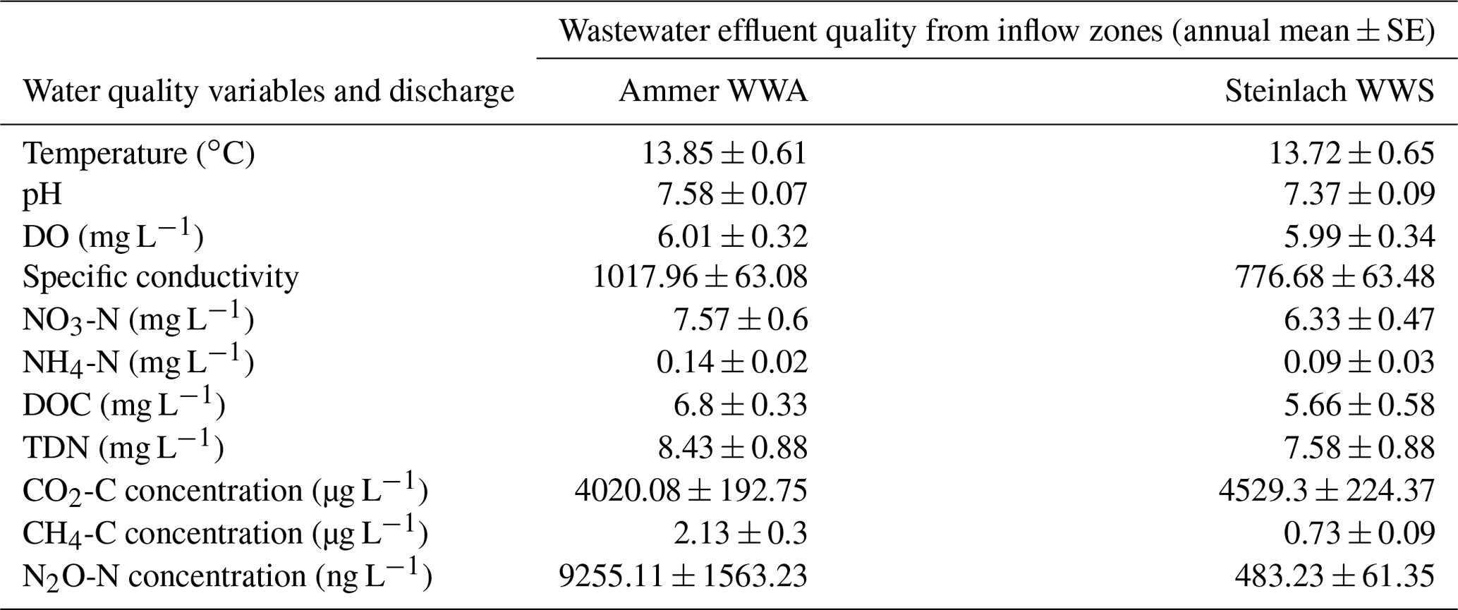
Table B2Seasonal means (+ SE) of water physico-chemical variables, gas concentration, and flux measured in the Loisach, Neckar, and Schwingbach catchments. The letters beside the means represent significant differences (p<0.05) amongst the seasons across the three catchments based on Tukey post hoc analyses from the linear mixed-effects model results (Table 2).
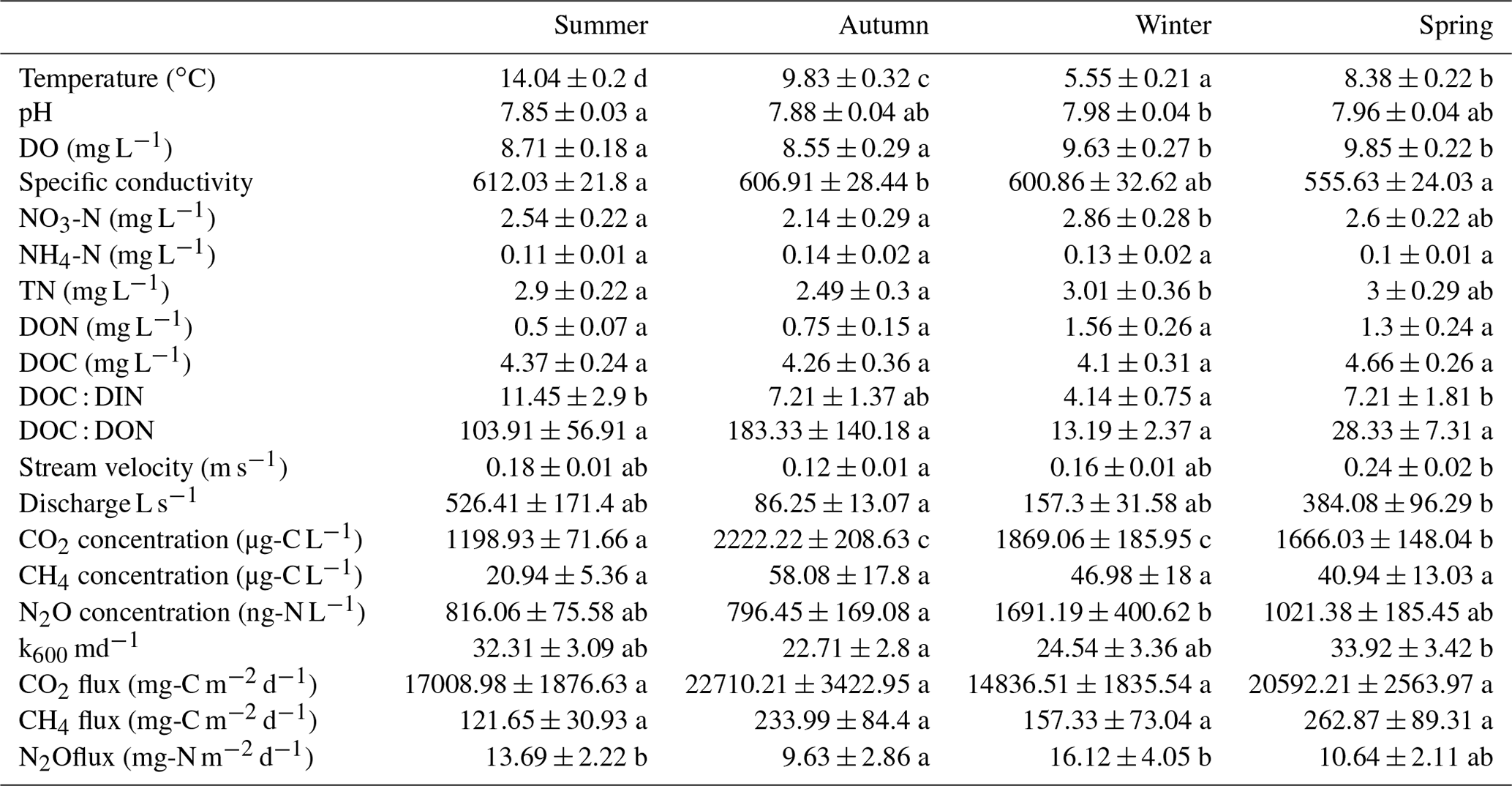
Table B3Annual mean ± standard errors of measured water physico-chemical variables, GHG concentration, and flux for land use classes in the Loisach (FOR: forest, WET: wetland, GRA: grassland, and DD: drainage ditches), the Neckar (FOR, FOR_S: forest + settlement, FOR_S_W: forest + settlement + wastewater inflow, CRP_S: cropland + settlement, and CRP_S_W: cropland + settlement + wastewater inflow), and the Schwingbach catchment (FOR, CRP: cropland and CRP_S). The number of observations in each land use class is represented by “n” in brackets. The letters beside the means represent significant differences (p<0.05) amongst the land use classes across the three catchments based on Tukey post hoc analyses from the linear mixed-effects model results (Table 2).
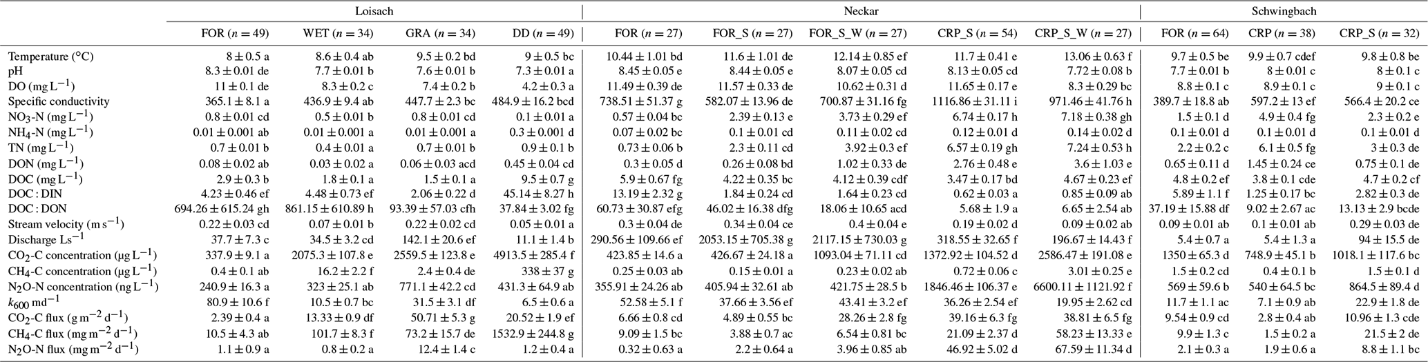
Table B4Indices highlighting the performance of the best-fit SEMs, which indicate significant interaction pathways of both direct and indirect drivers of in situ GHG concentrations in temperate streams, rivers, and drainage ditches. The goodness-of-fit index (GFI), comparative fit index (CF1), Tucker–Lewis index, standardized root mean square residual (SRMR), and root means squared error of approximation (RMSEA) are measures of model goodness of fit, while the parsimony fit index (PNFI) compares the best-fit model to the theoretical model.
The appendixes contain monthly, seasonal, and land-use-specific water physico-chemical and GHG data used in this research. All raw data (xlsx format) will be made available upon request to the corresponding author via email.
RMM, RK, GMG, CG, and KBB designed the field experiments. RK, KBB, TH, and LB provided the infrastructural funding, and RMM and EGW did the field and laboratory work. RMM did the statistical analysis, consulting with RK and GMG. RMM prepared the first draft of the paper, consulting with RK. All co-authors contributed to the final version.
The contact author has declared that none of the authors has any competing interests.
Publisher’s note: Copernicus Publications remains neutral with regard to jurisdictional claims in published maps and institutional affiliations.
This research was funded by the German academic exchange service (DAAD) as part of Ricky Mwangada Mwanake's doctoral studies. Infrastructure for the research was provided by the TERENO Bavarian Alps/Pre-Alps Observatory, funded by the Helmholtz Association and the Federal Ministry of Education and Research (BMBF). The authors would like to thank the entire laboratory staff at Karlsruhe Institute of Technology, Campus Alpin, Justus Liebig University Giessen, and the University of Tübingen for providing logistical support and supporting the gas and nutrient analyses. We also acknowledge the contributions of Alisson Kolar, Paul Levin Degott, Franz Weyerer, and Raphael Boehm during the field campaigns.
This research has been supported by the Deutscher Akademischer Austauschdienst (grant no. 57440921).
The article processing charges for this open-access publication were covered by the Karlsruhe Institute of Technology (KIT).
This paper was edited by Gwenaël Abril and reviewed by two anonymous referees.
Aho, K. S. and Raymond, P. A.: Differential response of greenhouse gas evasion to storms in forested and wetland streams, J. Geophys. Res.-Biogeo., 124, 649–662, https://doi.org/10.1029/2018JG004750, 2019.
Aho, K. S., Fair, J. H., Hosen, J. D., Kyzivat, E. D., Logozzo, L. A., Rocher-Ros, G., Weber, L. C., Yoon, B., and Raymond, P. A.: Distinct concentration-discharge dynamics in temperate streams and rivers: CO2 exhibits chemostasis while CH4 exhibits source limitation due to temperature control, Limnol. Oceanogr., 66, 3656–3668, https://doi.org/10.1002/lno.11906, 2021.
Aho, K. S., Fair, J. H., Hosen, J. D., Kyzivat, E. D., Logozzo, L. A., Weber, L. C., Yoon, B., Zarnetske, J. P., and Raymond, P. A.: An intense precipitation event causes a temperate forested drainage network to shift from N2O source to sink, Limnol. Oceanogr., 67, S242–S257, https://doi.org/10.1002/lno.12006, 2022.
Allen, G. H. and Pavelsky, T. M.: Global extent of rivers and streams, Science, 361, 585–588, https://doi.org/10.1126/science.aat0636, 2018.
Attermeyer, K., Casas-Ruiz, J. P., Fuss, T., Pastor, A., Cauvy-Fraunié, S., Sheath, D., Nydahl, A. C., Doretto, A., Portela, A. P., Doyle, B. C., and Simov, N.: Carbon dioxide fluxes increase from day to night across European streams, Commun. Earth Environ., 2, 118, https://doi.org/10.1038/s43247-021-00192-w, 2021.
Audet, J., Bastviken, D., Bundschuh, M., Buffam, I., Feckler, A., Klemedtsson, L., Laudon, H., Löfgren, S., Natchimuthu, S., Öquist, M., Peacock, M., and Wallin, M. B.: Forest streams are important sources for nitrous oxide emissions, Glob. Change Biol., 26, 629–641, https://doi.org/10.1111/gcb.14812, 2019.
Battin, T. J., Kaplan, L. A., Findlay, S., Hopkinson, C. S., Marti, E., Packman, A. I., Newbold, J. D., and Sabater, F.: Biophysical controls on organic carbon fluxes in fluvial networks, Nat. Geosci., 1, 95–100, https://doi.org/10.1038/ngeo101, 2008.
Battin, T. J., Lauerwald, R., Bernhardt, E. S., Bertuzzo, E., Gener, L. G., Hall Jr., R. O., Hotchkiss, E. R., Maavara, T., Pavelsky, T. M., Ran, L., and Raymond, P.: River ecosystem metabolism and carbon biogeochemistry in a changing world, Nature, 613, 449–459, https://doi.org/10.1038/s41586-022-05500-8, 2023.
Baulch, H. M., Dillon, P. J., Maranger, R., and Schiff, S. L.: Diffusive and ebullitive transport of methane and nitrous oxide from streams: Are bubble-mediated fluxes important?, J. Geophys. Res.-Biogeo., 116, G4, https://doi.org/10.1029/2011JG001656, 2011a.
Baulch, H. M., Schiff, S. L., Maranger, R., and Dillon, P. J.: Nitrogen enrichment and the emission of nitrous oxide from streams, Global Biogeochem. Cy., 25, 4, https://doi.org/10.1029/2011GB004047, 2011b.
Beaulieu, J. J., Arango, C. P., and Tank, J. L.: The effects of season and agriculture on nitrous oxide production in headwater streams, J. Environ. Qual., 38, 637–646, https://doi.org/10.2134/jeq2008.0003, 2009.
Begum, M. S., Bogard, M. J., Butman, D. E., Chea, E., Kumar, S., Lu, X., Nayna, O. K., Ran, L., Richey, J. E., Tareq, S. M., and Xuan, D. T.: Localized pollution impacts on greenhouse gas dynamics in three anthropogenically modified Asian river systems, J. Geophys. Res.-Biogeo., 126, 2020JG006124, https://doi.org/10.1029/2020JG006124, 2021.
Bodmer, P., Heinz, M., Pusch, M., Singer, G., and Premke, K.: Carbon dynamics and their link to dissolved organic matter quality across contrasting stream ecosystems, Sci. Total Environ., 553, 574–586, https://doi.org/10.1016/j.scitotenv.2016.02.095, 2016.
Bolleter, W. T., Bushman, C. J., and Tidwell, P. W.: Spectrophotometric determination of ammonia as indophenol, Anal. Chem., 33, 592–594, https://doi.org/10.1021/ac60172a034, 1961.
Borges, A. V., Darchambeau, F., Teodoru, C. R., Marwick, T. R., Tamooh, F., Geeraert, N., Omengo, F.O., Guérin, F., Lambert, T., Morana, C., and Okuku, E.: Globally significant greenhouse-gas emissions from African inland waters, Nat. Geosci., 8, 637–642, https://doi.org/10.1038/ngeo2486, 2015.
Borges, A. V., Darchambeau, F., Lambert, T., Bouillon, S., Morana, C., Brouyère, S., Hakoun, V., Jurado, A., Tseng, H.C., Descy, J. P., and Roland, F. A.: Effects of agricultural land use on fluvial carbon dioxide, methane and nitrous oxide concentrations in a large European river, the Meuse (Belgium), Sci. Total Environ., 610/611, 342–355, https://doi.org/10.1016/j.scitotenv.2017.08.047, 2018.
Borges, A. V., Darchambeau, F., Lambert, T., Morana, C., Allen, G. H., Tambwe, E., Toengaho Sembaito, A., Mambo, T., Nlandu Wabakhangazi, J., Descy, J. P., and Teodoru, C. R.: Variations in dissolved greenhouse gases (CO2, CH4, N2O) in the Congo river network overwhelmingly driven by fluvial-wetland connectivity, Biogeosciences, 16, 3801–3834, https://doi.org/10.5194/bg-16-3801-2019, 2019.
Crawford, J. T., Dornblaser, M. M., Stanley, E. H., Clow, D. W., and Striegl, R. G.: Source limitation of carbon gas emissions in high-elevation mountain streams and lakes, J. Geophys. Res.-Biogeo., 120, 952–964, https://doi.org/10.1002/2014JG002861, 2015.
Deirmendjian, L., Anschutz, P., Morel, C., Mollier, A., Augusto, L., Loustau, D., Cotovicz Jr., L.C., Buquet, D., Lajaunie, K., Chaillou, G., and Voltz, B.: Importance of the vegetation-groundwater-stream continuum to understand transformation of biogenic carbon in aquatic systems – A case study based on a pine-maize comparison in a lowland sandy watershed (Landes de Gascogne, SW France), Sci. Total Environ., 661, 613–629, https://doi.org/10.1016/j.scitotenv.2019.01.152, 2019.
Dinsmore, K. J., Wallin, M. B., Johnson, M. S., Billett, M. F., Bishop, K., Pumpanen, J., and Ojala, A.: Contrasting CO2 concentration discharge dynamics in headwater streams: A multi-catchment comparison, J. Geophys. Res.-Biogeo., 118, 445–461, https://doi.org/10.1002/jgrg.20047, 2013.
Drake, T. W., Raymond, P. A., and Spencer, R. G.: Terrestrial carbon inputs to inland waters: A current synthesis of estimates and uncertainty, Limnol. Oceanogr. Lett., 3, 132–142, https://doi.org/10.1002/lol2.10055, 2018.
Galantini, L., Lapierre, J. F., and Maranger, R.: How are greenhouse gases coupled across seasons in a large temperate river with differential land use?, Ecosystems, 24, 2007–2027, 2021.
Gomez-Gener, L., Rocher-Ros, G., Battin, T., Cohen, M. J., Dalmagro, H. J., Dinsmore, K. J., Drake, T. W., Duvert, C., Enrich-Prast, A., Horgby, Å., and Johnson, M. S.: Global carbon dioxide efflux from rivers enhanced by high nocturnal emissions, Nat. Geosci., 14, 289–294, https://doi.org/10.1038/A41561-021-00722-3, 2021.
Glaser, C., Schwientek, M., Junginger, T., Gilfedder, B. S., Frei, S., Werneburg, M., Zwiener, C., and Zarfl, C.: Comparison of environmental tracers including organic micropollutants as groundwater exfiltration indicators into a small river of a karstic catchment, Hydrol. Process., 34, 4712–4726, https://doi.org/10.1002/hyp.13909, 2020.
Gore, J. A.: Discharge measurements and streamflow analysis, in: Methods in stream ecology, edited by: Hauer, F. R. and Lamberti, G. A., 2nd Edn., Chap. 3, 51–77, Cambridge, MA, Academic Press, https://doi.org/10.1016/B978-012332908-0.50005-X, 2007.
Hall Jr., R. O. and Ulseth, A. J.: Gas exchange in streams and rivers, Wiley Interdisciplinary Reviews: Water, 7, e1391, https://doi.org/10.1002/wat2.1391, 2020.
Herreid, A. M., Wymore, A. S., Varner, R. K., Potter, J. D., and McDowell, W. H.: Divergent controls on stream greenhouse gas concentrations across a land-use gradient, Ecosystems, 24, 1299–1316, https://doi.org/10.1007/A10021-020-00584-7, 2021.
Holtan-Hartwig, L., Dörsch, P., and Bakken, L. R.: Low temperature control of soil denitrifying communities: kinetics of N2O production and reduction, Soil Biol. Biochem., 34, 1797–1806, https://doi.org/10.1016/S0038-0717(02)00169-4, 2002.
Horgby, Å., Boix Canadell, M., Ulseth, A. J., Vennemann, T. W., and Battin, T. J.: High-resolution spatial sampling identifies groundwater as driver of CO2 dynamics in an Alpine stream network, J. Geophys. Res.-Biogeo., 124, 1961–1976, https://doi.org/10.1029/2019JG005047, 2019.
Hotchkiss, E. R., Hall Jr., R. O., Sponseller, R. A., Butman, D., Klaminder, J., Laudon, H., Rosvall, M., and Karlsson, J.: Sources of and processes controlling CO2 emissions change with the size of streams and rivers, Nat. Geosci., 8, 696–699, https://doi.org/10.1038/ngeo2507, 2015.
Hu, M., Chen, D., and Dahlgren, R. A.: Modeling nitrous oxide emission from rivers: a global assessment, Glob. Change Biol., 22, 3566–3582, https://doi.org/10.1111/gcb.13351, 2016.
IPCC (Intergovernmental Panel on Climate Change): Climate change 2013–the physical science basis: Working group I contribution to the fifth assessment report of the Intergovernmental Panel on Climate Change, Cambridge: Cambridge University Press, https://doi.org/10.1017/CBO9781107415324, 2014.
Kuhn, C., Bettigole, C., Glick, H. B., Seegmiller, L., Oliver, C. D., and Raymond, P.: Patterns in stream greenhouse gas dynamics from mountains to plains in northcentral Wyoming, J. Geophys. Res.-Biogeo., 122, 2173–2190, https://doi.org/10.1002/2017JG003906, 2017.
Lambert, T., Bouillon, S., Darchambeau, F., Morana, C., Roland, F. A. E., Descy, J., and Borges, A. V.: Effects of human land use on the terrestrial and aquatic sources of fluvial organic matter in a temperate river basin (The Meuse River, Belgium), Biogeochemistry, 136, 191–211, 2017.
Li, M., Peng, C., Zhang, K., Xu, L., Wang, J., Yang, Y., Li, P., Liu, Z., and He, N.: Headwater stream ecosystem: an important source of greenhouse gases to the atmosphere, Water Res., 190, 116738, https://doi.org/10.1016/j.watres.2020.116738, 2021.
Marescaux, A., Thieu, V., and Garnier, J.: Carbon dioxide, methane and nitrous oxide emissions from the human-impacted Seine watershed in France, Sci. Total Environ., 643, 247–259, https://doi.org/10.1016/j.scitotenv.2018.06.151, 2018.
McDowell, M. J. and Johnson, M. S.: Gas transfer velocities evaluated using carbon dioxide as a tracer show high streamflow to be a major driver of total CO2 evasion flux for a headwater stream, J. Geophys. Res.-Biogeo., 123, 2183–2197, https://doi.org/10.1029/2018JG004388, 2018.
Mwanake, R. M., Gettel, G. M., Aho, K. S., Namwaya, D. W., Masese, F. O., Butterbach-Bahl, K., and Raymond, P. A.: Land use, not stream order, controls N2O concentration and flux in the upper Mara River basin, Kenya, J. Geophys. Res.-Biogeo., 124, 3491–3506, https://doi.org/10.1029/2019jg005063, 2019.
Mwanake, R. M., Gettel, G. M., Ishimwe, C., Wangari, E. G., Butterbach-Bahl, K., and Kiese, R.: Basin-scale estimates of greenhouse gas emissions from the Mara River, Kenya: Importance of discharge, stream size, and land use/land cover, Limnol. Oceanogr., 67, 1776–1793, https://doi.org/10.1002/lno.12166, 2022.
Mwanake, R. M., Gettel, G. M., Wangari, E. G., Butterbach-Bahl, K., and Kiese, R.: Interactive effects of catchment mean water residence time and agricultural area on water physico-chemical variables and GHG saturations in headwater streams, Front. Water, 5, 1220544, https://doi.org/10.3389/frwa.2023.1220544, 2023.
O'Donnell, J. A., Aiken, G. R., Kane, E. S., and Jones, J. B.: Source water controls on the character and origin of dissolved organic matter in streams of the Yukon River basin, Alaska, J. Geophys. Res.-Biogeo., 115, G3, https://doi.org/10.1029/2009JG001153, 2010.
Park, J. H., Nayna, O. K., Begum, M. S., Chea, E., Hartmann, J., Keil, R. G., Kumar, S., Lu, X., Ran, L., Richey, J. E., and Sarma, V. V.: Reviews and syntheses: Anthropogenic perturbations to carbon fluxes in Asian river systems – concepts, emerging trends, and research challenges, Biogeosciences, 15, 3049–3069, https://doi.org/10.5194/bg-15-3049-2018, 2018.
Patton, C. J. and Kryskalla, J. R.: Colorimetric determination of nitrate plus nitrite in water by enzymatic reduction, automated discrete analyzer methods, US Geological Survey, Techniques and Methods, Book 5, 34 pp., https://doi.org/10.3133/tm5B8, 2011.
Peacock, M., Granath, G., Wallin, M. B., Högbom, L., and Futter, M. N.: Significant Emissions From Forest Drainage Ditches – An Unaccounted Term in Anthropogenic Greenhouse Gas Inventories?, J. Geophys. Res.-Biogeo., 126, 10, https://doi.org/10.1029/2021JG006478, 2021a.
Peacock, M., Audet, J., Bastviken, D., Futter, M. N., Gauci, V., Grinham, A., Harrison, J. A., Kent, M. S., Kosten, S., Lovelock, C. E., and Veraart, A. J.: Global importance of methane emissions from drainage ditches and canals, Environ. Res. Lett., 16, 044010, https://doi.org/10.1088/1748-9326/abeb36, 2021b.
Quick, A. M., Reeder, W. J., Farrell, T. B., Tonina, D., Feris, K. P., and Benner, S. G.: Nitrous oxide from streams and rivers: A review of primary biogeochemical pathways and environmental variables, Earth-Sci. Rev., 191, 224–262, https://doi.org/10.1016/j.earscirev.2019.02.021, 2019.
Raymond, P. A., Zappa, C. J., Butman, D., Bott, T. L., Potter, J., Mulholland, P., Laursen, A. E., McDowell, W. H., and Newbold, D.: Scaling the gas transfer velocity and hydraulic geometry in streams and small rivers, Limnol. Oceanogr., 2, 41–53, https://doi.org/10.1215/21573689-1597669, 2012.
Reay, D. S., Smith, K. A., and Edwards, A. C.: Nitrous oxide emission from agricultural drainage waters, Glob. Change Biol., 9, 195–203, https://doi.org/10.1046/j.1365-2486.2003.00584.x, 2003.
Rocher-Ros, G., Sponseller, R. A., Lidberg, W., Mörth, C. M., and Giesler, R.: Landscape process domains drive patterns of CO2 evasion from river networks, Limnol. Oceanogr. Lett., 4, 87–95, https://doi.org/10.1002/lol2.10108, 2019.
Schade, J. D., Bailio, J., and McDowell, W. H.: Greenhouse gas flux from headwater streams in New Hampshire, USA: Patterns and drivers, Limnol. Oceanogr., 61, 165–17, https://doi.org/10.1002/lno.10337, 2016.
Schrier-Uijl, A. P., Veraart, A. J., Leffelaar, P. A., Berendse, F., and Veenendaal, E. M.: Release of CO2 and CH4 from lakes and drainage ditches in temperate wetlands, Biogeochemistry, 102, 265–279, https://doi.org/10.1007/A10533-010-9440-7, 2011.
Schumacker, R. E. and Lomax, R. G.: A Beginner's Guide to Structural Equation Modeling, 4th Edn., New York, Routledge, https://doi.org/10.4324/9781315749105, 2015.
Sebestyen, S. D., Boyer, E. W., Shanley, J. B., Kendall, C., Doctor, D. H., Aiken, G. R., and Ohte, N.: Sources, transformations, and hydrological processes that control stream nitrate and dissolved organic matter concentrations during snowmelt in an upland forest, Water Resour. Res., 44, 12, https://doi.org/10.1029/2008WR006983, 2008.
Shelley, F., Grey, J., and Trimmer, M.: Widespread methanotrophic primary production in lowland chalk rivers, Proc. Roy. Soc. B, 281, 1783, https://doi.org/10.1098/rspb.2013.2854, 2014.
Stanley, E. H, Casson, N. J., Christel, S. T., Crawford, J. T., Loken, L. C., and Oliver, S. K.: The ecology of methane in streams and rivers: patterns, controls, and global significance, Ecol. Monogr., 86, 146–171, https://doi.org/10.1890/15-1027, 2016.
Strahler, A. N.: Hypsometric (area-altitude) analysis of erosional topography, GSA Bull., 63, 1117–1142, https://doi.org/10.1130/0016-7606(1952)63[1117:HAAOET]2.0.CO;2, 1952.
Turner, P. A., Griffis, T. J., Lee, X., Baker, J. M., Venterea, R. T., and Wood, J. D.: Indirect nitrous oxide emissions from streams within the US Corn Belt scale with stream order, P. Natl. Acad. Sci. USA, 112, 9839–9843, https://doi.org/10.1073/pnas.1503598112, 2015.
Wallin, M. B., Campeau, A., Audet, J., Bastviken, D., Bishop, K., Kokic, J., Laudon, H., Lundin, E., Löfgren, S., Natchimuthu, S., and Sobek, S.: Carbon dioxide and methane emissions of Swedish low-order streams – A national estimate and lessons learnt from more than a decade of observations, Limnol. Oceanogr., 3, 156–167, https://doi.org/10.1002/lol2.10061, 2018.
Wallin, M. B., Audet, J., Peacock, M., Sahlée, E., and Winterdahl, M.: Carbon dioxide dynamics in an agricultural headwater stream driven by hydrology and primary production, Biogeosciences, 17, 2487–2498, https://doi.org/10.5194/bg-17-2487-2020, 2020.
Wang, D., Ye, W., Wu, G., Li, R., Guan, Y., Zhang, W., Wang, J., Shan, Y., and Hubacek, K.: Greenhouse gas emissions from municipal wastewater treatment facitlities in China from 2006 to 2019, Sci. Data, 9, 317, https://doi.org/10.1038/s41597-022-01439-7, 2022.
Wangari, E. G., Mwanake, R. M., Kraus, D., Werner, C., Gettel, G. M., Kiese, R., Breuer, L., Butterbach-Bahl, K., and Houska, T.: Number of chamber measurement locations for accurate quantification of landscape-scale greenhouse gas fluxes: Importance of land use, seasonality, and greenhouse gas type, J. Geophys. Res.-Biogeo., 127, 9, https://doi.org/10.1029/2022JG006901, 2022.
Winkler, K., Fuchs, R., Rounsevell, M., and Herold, M.: Global land use changes are four times greater than previously estimated, Nat. Commun., 12, 1–10, 2021.
Zhang, L., Xia, X., Liu, S., Zhang, S., Li, S., Wang, J., Wang, G., Gao, H., Zhang, Z., Wang, Q., and Wen, W.: Significant methane ebullition from alpine permafrost rivers on the East Qinghai–Tibet Plateau, Nat. Geosci., 13, 349–354, 2020.
Zhang, W., Li, H., Xiao, Q., and Li, X.: Urban rivers are hotspots of riverine greenhouse gas (N2O, CH4, CO2) emissions in the mixed-landscape chaohu lake basin, Water Res., 189, 116624, https://doi.org/10.1016/j.watres.2020.116624, 2021.
Zhou, J., Liu, G., Meng, Y., Xia, C., Chen, K., and Chen, Y.: Using stable isotopes as tracer to investigate hydrological condition and estimate water residence time in a plain region, Chengdu, China, Sci. Rep., 11, 1–12, https://doi.org/10.1038/s41598-021-82349-3, 2021.