Sources and sinks of carbonyl sulfide inferred from tower and mobile atmospheric observations in the Netherlands

Carbonyl sulfide (COS) is a promising tracer for the estimation of terrestrial ecosystem gross primary production (GPP). However, understanding its non-GPP-related sources and sinks, e.g., anthropogenic sources and soil sources and sinks, is also critical to the success of the approach. Here we infer the regional sources and sinks of COS using continuous in situ mole fraction profile measurements of COS along the 60 m tall Lutjewad tower (1 m a.s.l.; 53^∘24^′ N, 6^∘21^′ E) in the Netherlands. To identify potential sources that caused the observed enhancements of COS mole fractions at Lutjewad, both discrete flask samples and in situ measurements in the province of Groningen were made from a mobile van using a quantum cascade laser spectrometer (QCLS). We also simulated the COS mole fractions at Lutjewad using the Stochastic Time-Inverted Lagrangian Transport (STILT) model combined with emission inventories and plant uptake fluxes. We determined the nighttime COS fluxes to be $-\mathrm{3.0}\pm \mathrm{2.6}$ pmol m⁻² s⁻¹ using the radon-tracer correlation approach and Lutjewad observations. Furthermore, we identified and quantified several COS sources, including biodigesters, sugar production facilities and silicon carbide production facilities in the province of Groningen. Moreover, the simulation results show that the observed COS enhancements can be partially explained by known industrial sources of COS and CS₂, in particular from the Ruhr Valley (51.5^∘ N, 7.2^∘ E) and Antwerp (51.2^∘ N, 4.4^∘ E) areas. The contribution of likely missing anthropogenic sources of COS and CS₂ in the inventory may be significant. The impact of the identified sources in the province of Groningen is estimated to be negligible in terms of the observed COS enhancements. However, in specific conditions, these sources may influence the measurements in Lutjewad. These results are valuable for improving our understanding of the sources and sinks of COS, contributing to the use of COS as a tracer for GPP.

1 Introduction

Interest in the budget of carbonyl sulfide (COS) has grown over the last decade due to the close relation of COS and carbon dioxide (CO₂) vegetative uptake. The two gases follow a similar uptake pathway from the leaf boundary layer up to the site of reaction in the plant (Stimler et al., 2010). COS therefore provides a means to separate the concurrent uptake of gross primary productivity (GPP) and respiration flux of CO₂ (Campbell et al., 2008; Montzka et al., 2007). Those individual fluxes can otherwise not be measured directly at scales larger than the leaf scale. Besides the interest in COS as a tracer for GPP, COS is also of interest in the stratosphere as it plays a role in the formation of the stratospheric sulfate aerosol layer, which has an overall cooling effect on the Earth's climate (Brühl et al., 2012).

Mole fractions of COS in the atmosphere range between 350 and 550 parts per trillion (ppt) globally. The vegetative uptake of COS is the largest sink in the atmospheric COS budget, followed by uptake by soils (Berry et al., 2013; Whelan et al., 2018). The main sources of COS are anthropogenic emissions, the ocean, wetlands and biomass burning. Anthropogenic emissions of COS can be either direct emissions of COS (e.g., coal combustion, aluminum smelting, pigment and paper industry) or indirect through emissions of CS₂ (e.g., rayon production, agricultural chemicals and tire wear), which can be oxidized to COS (Zumkehr et al., 2018). Unfortunately, the current COS budget has large uncertainties, and lacks COS sources to balance the sinks, mainly due to uncertainties in the contribution of the tropical ocean and anthropogenic emissions (Whelan et al., 2018).

The long-term COS record presented by Montzka et al. (2007) gave insight into the seasonality of COS mole fractions: it showed that the COS mole fraction is largely influenced by uptake by the biosphere in the Northern Hemisphere and by oceanic emissions in the Southern Hemisphere. This dataset is still being updated and can be visualized online (NOAA, 2023). These measurements were made using discrete flask samples (one to five samples per month) that were analyzed by a gas chromatographic and mass spectrometer. However, optical instruments that are capable of making high-frequency (1 to 10 Hz) in situ simultaneous measurements of COS and CO₂ (Stimler et al., 2009) are available, e.g., a quantum cascade laser spectrometer (QCLS). This creates opportunities to advance our understanding of the COS sources and sinks through flux measurements using the eddy-covariance technique and soil and branch chamber measurements (Berkelhammer et al., 2014; Commane et al., 2015; Kitz et al., 2017; Maseyk et al., 2014; Sun et al., 2018; Vesala et al., 2022; Wehr et al., 2017; Yang et al., 2018) and through atmospheric mole fraction measurements within the continental and marine boundary layer (Belviso et al., 2016, 2020; Commane et al., 2013; Kooijmans et al., 2016; Lennartz et al., 2017). Moreover, this instrument enabled the collection of in situ data from a mobile van, which made it possible to identify COS sources directly at their emission sites.

The tropospheric COS molar fraction is only monitored at a few sites in Europe. Among these, four monitoring sites are located in western Europe, within 48 and 53^∘ N: Mace Head, Ireland (Montzka et al., 2007); Gif-sur-Yvette and Traînou, France (Belviso et al., 2022b); and Lutjewad, the Netherlands (Kooijmans et al., 2016). Moreover, COS has been recently monitored discontinuously in Utrecht, the Netherlands (Baartman et al., 2022). The observations in these studies show higher autumn and winter COS molar fractions in the Netherlands than at Mace Head, Ireland, and at Gif-sur-Yvette and Traînou, France. This calls for a more thorough investigation of possible local sources in the Netherlands at a local and regional scale. A proper assessment of local sources is also necessary to evaluate the performance of existing databases, such as the one realized by Zumkehr et al. (2018). A recent effort has been reported by Belviso et al. (2023) at a sub-regional level in France.

This study aims to investigate the processes that impact the atmospheric COS mole fractions at Lutjewad and to infer the influence of local COS sources on the Lutjewad measurements. This has been realized with continuous atmospheric mole fraction observations of COS, CO₂ and carbon monoxide (CO) at the 60 m tall tower and with discrete flask and continuous in situ measurements of COS, CO₂, CH₄, N₂O and CO from a mobile van in the province of Groningen in the Netherlands. Moreover, atmospheric COS and CO₂ mole fractions at Lutjewad were simulated for the period of January and February 2018, using the Stochastic Time-Inverted Lagrangian Transport (STILT) model. Finally, we estimated nighttime COS ecosystem fluxes and anthropogenic COS emissions from identified local sources based on atmospheric mole fraction measurements of COS.

2 Methodology

2.1 Measurement sites

2.1.1 Stationary measurements

Profile measurements were performed at the Lutjewad atmospheric monitoring station in the Netherlands (53^∘24^′ N, 6^∘21^′ E). The Lutjewad station is located at the north coast of the Netherlands in front of the Wadden Sea (largely consisting of tidal mudflats). The first kilometer towards the north is covered by salt marshes. Towards the south, the area is used for agriculture. Much of the land in the area is reclaimed from the sea with the use of dikes since the 15th century. The agricultural land around the Lutjewad station was reclaimed from the Wadden Sea in the 19th and early in the 20th century; therefore, the soil consists of clay that originates from the sea. The station is located next to the dike (which is 7 m high) of the Wadden Sea and consists of a 60 m tall tower. The area is sparsely populated: the closest village is Hornhuizen (∼200 inhabitants) at a distance of 1.3 km towards the south; the closest city is Groningen (∼ 200 000 inhabitants) at a distance of 25 km towards the southeast. A small ferry port is 10 km towards the west of the station. Farmlands around the measurement station are planted with seed potatoes, sugar beets and winter wheat. An aluminum smelting factory is 40 km towards the southeast (Damco Aluminium; 53^∘18^′ N, 6^∘58^′ E) which lies within the Delfzijl–Farmsum industrial area. Regionally, there are several aluminum and chemical facilities at 250 km distance in the German Ruhr area (e.g., Trimet Aluminium, Hydro) that may be a source of COS.

2.1.2 Mobile flask and in situ measurements

Several facilities were investigated for their potential COS emissions in the surroundings of Lutjewad, including both known COS emitters from literature, such as coal-related industries (Campbell et al., 2015; Zumkehr et al., 2018), and potential new sources, such as organic waste treatment plants (Aston and Douglas, 1981; Smet et al., 1998). These locations and their source types are summarized in Table 1, with their locations shown in Fig. 1.

Table 1 Possible sources of COS according to the retrieved literature.

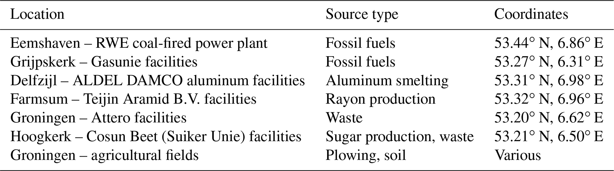
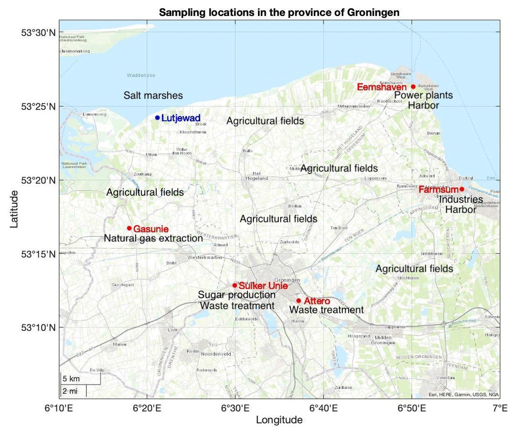
Figure 1 Location of Lutjewad and of the sampling locations in the province of Groningen (the Netherlands). The map also shows the major features of the sampling locations and their surrounding areas. Only the locations where emissions were detected are described in the text.

2.2 Measurements of COS, CO₂ and CO

2.2.1 Stationary measurements

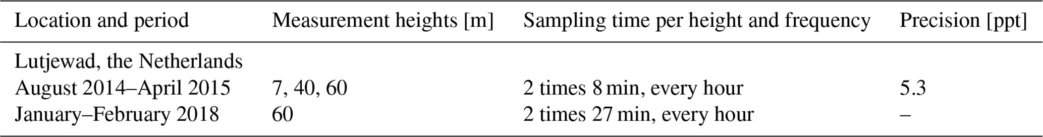
A QCLS was used to measure dry mole fractions of COS, CO₂, CO and H₂O at different heights of the Lutjewad tower between 2014 and 2018 (Table 2). The measured data were first presented in Kooijmans et al. (2016, their Fig. 12) for the period between August 2014 and April 2015. The setup of the QCLS is described in detail in Kooijmans et al. (2016). In summary, the QCLS sampled air from different heights (see Table 2) and the different sampling lines (Synflex Dekabon or Teflon) were switched with a multi-position Valco valve (VICI, Valco Instruments Co. Inc.). The sampling time differed per period (Table 2). A reference cylinder was measured every 0.5 h to correct for instrument drift and to calibrate the measurements to the common scales. Specifically, the reference cylinders were calibrated against two NOAA Earth System Research Laboratories (ESRL) standards for COS (NOAA-2004 scale) and CO₂ (WMO-X2007 CO₂ scale) at the University of Groningen (Kooijmans et al., 2016). The measurements had to be corrected for a leaking solenoid valve for the period between August 2014 and January 2015. This was done by comparing the CO₂ measurements with measurements from a collocated cavity ring-down spectrometer (Picarro Inc. model G2401-m) and applying a similar dilution factor to all gas species (see details in Kooijmans et al., 2016). A target cylinder was measured once every hour in all periods except for the measurements in Lutjewad in January–February 2018. Kooijmans et al. (2016) gave an overview of all uncertainty contributions that are relevant for obtaining accurate and precise COS mole fractions, that is, the repeatability of the NOAA scale (2.1 ppt), calibration of reference standards and ambient air samples (2.8 ppt), water vapor correction (2.9 ppt), and measurement precision. The measurement precision (defined as the standard deviation over minute-averaged target cylinder measurements after drift correction with reference measurements) has changed over the years; the average precision for the 2014–2015 period was 5.3 ppt.

Field standard cylinders are calibrated against NOAA standards in the laboratory before and after each measurement period to test for drift in the molar fraction of gas species. The COS mole fraction measurements of nine cylinders are available, and five cylinders changed by less than 2.5 ppt a⁻¹, two cylinders decreased by ∼ 10 ppt a⁻¹ and two cylinders decreased by ∼ 30 ppt a⁻¹. The four cylinders that drifted more than 10 ppt a⁻¹ were not used as reference cylinders in the data processing. All of the cylinders were uncoated aluminum cylinders, which, according to experience at NOAA, are more prone to COS mole fraction drift than Aculife-treated aluminum cylinders.

To investigate COS seasonal cycle amplitude in Lutjewad, besides the in situ measurements, we also measured flasks that were sampled at 60 m between December 2013 and February 2016 with an average of four samples per month. Of the flask samples, 81 % were taken at noon CET (UTC+1). For a detailed description of the measurement procedure, see Kooijmans et al. (2016). The flask measurements of COS mole fractions were used together with the in situ measurements in Lutjewad to construct a seasonal fit to the data. We constructed a seasonal fit to the 60 m COS and CO₂ mole fractions from Lutjewad. The non-linear least-squares fit of COS mole fractions is shown in Fig. S2 of the Supplement, and details are explained in the accompanying text.

Table 2 Measurement periods at the Lutjewad site with an overview of the measurement heights, sampling time and 1 min measurement precision based on target cylinder measurements (in January–February 2018 in Lutjewad, no target measurements were made).

2.2.2 Mobile flask and in situ measurements

The mobile and in situ investigation of the sources described in Sect. 2.1 was performed in September and October 2019. Firstly, discrete samples were collected in flasks and analyzed on a QCLS, which allowed the simultaneous analysis of COS, CO, CO₂, CH₄ and N₂O. Afterwards, a van was equipped as a mobile sampling station to realize in situ continuous analysis and allow immediate detection of COS enhancements. A QCLS was placed in the inside of the van, where electricity was supplied by three 115 A h 12 V lead acid batteries via a Mean Well TS-700 inverter. The instrument pulled air through a sampling line, with its inlet placed on the top of the vehicle. The sampling line was equipped with a reverse cup as a rain guard and a Nafion dryer to remove most water vapor from the air samples. During sampling, GPS live data synchronized with the QCLS time log were collected. Generally, this method allowed real-time investigation of the areas of interest, enabling the understanding of the spatial distribution of trace gas concentration.

2.3 Nighttime ecosystem flux in Lutjewad

Nighttime fluxes of COS and CO₂ are estimated for the Lutjewad area based on the radon-tracer method, similarly to the calculation of nighttime fluxes in Hyytiälä by Kooijmans et al. (2017). Measurements of ²²²Rn can be used to calculate fluxes of other gases because ²²²Rn is produced in the soil with a constant rate and it diffuses through the soil into the air. Once it is in the atmosphere, it is only affected by radioactive decay and by the effect of atmospheric mixing. The nighttime mole fractions of gases be either enriched (in the case of dominant sources) or depleted (in the case of dominant sinks) in a shallower nocturnal boundary layer compared to the daytime boundary layer. This means that, when the ²²²Rn exhalation rate (F_Rn) is known, the surface fluxes of another gas (in this case of COS (F_COS) and CO₂ ($F_{{\mathrm{CO}}_{\mathrm{2}}}$)) can be determined from the mole fraction changes of the gas (ΔCOS and ΔCO₂) over the night relative to the mole fraction change of ²²²Rn (Δ²²²Rn): e.g., $F_{\mathrm{COS}}=F_{\mathrm{Rn}}\cdot (\mathrm{\Delta }\mathrm{COS}/{\mathrm{\Delta }}^{\mathrm{222}}\mathrm{Rn})$ (Belviso et al., 2013, 2020; Schmidt et al., 1996; van der Laan et al., 2009). F_Rn was determined for the Lutjewad area in different measurement and modeling studies, an overview of which is given in van der Laan et al. (2016). In these studies, F_Rn varied between 2.3 and 5.1 mBq m⁻² s⁻¹. We will use the average over these studies, 3.7 mBq m⁻² s⁻¹, with a standard deviation of 1.2 mBq m⁻² s⁻¹. The ²²²Rn measurements in Lutjewad are made with an ANSTO dual-flow-loop two-filter detector (Whittlestone and Zahorowski, 1998). Details about the measurement procedure are described in van der Laan et al. (2009). COS and CO₂ fluxes are only calculated for nights when at least seven data points are available, where the R² values between ²²²Rn and COS (CO₂) mole fractions are larger than 0.4 (0.5), and where the standard error of the flux (based on the uncertainty in the slope between ²²²Rn and COS or CO₂ mole fractions) is smaller than 4 pmol m⁻² s⁻¹ (COS) and 1.5 µmol m⁻² s⁻¹ (CO₂). The calculations are limited to nighttime data since the ²²²Rn method is based on vertical gradients and would therefore be difficult to apply with convective conditions. Furthermore, the uncertainties in the radon-tracer method largely result from the uncertainty in F_Rn. The flux uncertainty is therefore calculated as the quadrature sum of the uncertainty in the slope and in F_Rn (1.2 mBq m⁻² s⁻¹).

2.4 Simulations of COS mole fractions

To understand the influence of natural and anthropogenic COS sources on the concentration measurements at Lutjewad, atmospheric transport simulations were performed to obtain COS mole fractions at the station. The simulation covers the period from January to February 2018, given the availability for both observations and models data and unusually high COS molar fractions (see Sect. 3.2) for this period. This analysis aims to disentangle the influence of local and regional sources on these observations. To simulate the enhancements from the COS background concentrations, the Stochastic Time-Inverted Lagrangian Transport (STILT) model (Lin et al., 2003), driven by ECMWF Integrated Forecasting System (IFS) operational analysis at a 0.25^∘ × 0.25^∘ resolution, was combined with COS biosphere and soil fluxes from the Simple Biosphere Model, version 4 (SiB4) (Kooijmans et al., 2021), and with the anthropogenic emission database by Zumkehr et al. (2018). The COS background was estimated using the endpoint of the STILT model trajectories in the analysis domain and the derived 3D concentration fields from the Transport Model 5 four-dimensional variational model (TM5-4DVAR) inversions (Ma et al., 2021).

The STILT model establishes the link between the emissions in the upwind influencing area and the measurements at a defined location and time. This is realized by releasing particles to the atmosphere that are driven by meteorological winds and transported backwards in time to determine the origin of air parcels influencing the measurements. Each simulation run releases 100 particles from the Lutjewad station, at a height of 60 m. The transport of these particles is reconstructed within the selected domain (latitude 34.0–73.5^∘ N, longitude 20.0^∘ W–45.5^∘ E, to cover Europe) in 3 h time steps over 10 d back in time. For this study case, the period covers a total of 472 time steps between 1 January 2018 at midnight and 28 February 2018 at 21:00 CET (UTC+1). Depending on the number, the location and the height of the particles, the model computes footprints in ppm (µmol m⁻² s⁻¹)⁻¹, at a 0.1^∘ × 0.1^∘ resolution, indicating the influence of specific areas on the final measurements. An example is shown in Fig. 2c. The resulting footprint becomes more dispersed and its total value becomes smaller for each time step back in time, and it is thus less influential on the simulated concentration at the receptor. In this analysis, footprints are reliably negligible (their sum over the selected domain being at least 3 orders of magnitude lower than at the beginning of the simulation) after 8 to 9 d. Therefore, the simulation time span is set to 10 d to confidently cover all the potentially significant footprint values.

The SiB4 and the anthropogenic emission databases include gridded COS fluxes (pmol m⁻² s⁻¹) and were interpolated to grids of 0.1^∘ × 0.1^∘ to match the STILT footprints. Biospheric COS fluxes are defined for each 3 h time step, depending on time of the day and seasonality. In the considered period, these fluxes are negative, mainly due to COS uptake by soils. Anthropogenic fluxes are assumed to be constant over time and include both direct and indirect COS emissions. Anthropogenic COS emissions maps are shown in Fig. 2a–b. The indirect emissions are accounted for as CS₂ fluxes. The conversion of CS₂ to COS is computed with two different scenarios, considering a 3 d exponential (Khan et al., 2017) and a 10 d exponential conversion rate (Ma et al., 2021), with a reaction yield of 0.87 (Ma et al., 2021; Zumkehr et al., 2018). Therefore, the indirect COS fluxes are calculated for each time step i back in time (maximum 240 h or 10 d) as described by Eq. (1). All COS fluxes are then multiplied by footprint values f to obtain the relative COS contributions: $\mathrm{\Delta }{\mathrm{COS}}_i=F_i\cdot f$. Consequently, the COS enhancement at the receptor ΔCOS consists of the contribution from the biospheric fluxes ΔCOS_bio, the contribution from the constant direct anthropogenic emissions $\mathrm{\Delta }{\mathrm{COS}}_{\mathrm{ant}}^{\mathrm{dir}}$ and the contribution from time-varying indirect anthropogenic fluxes $\mathrm{\Delta }{\mathrm{COS}}_{\mathrm{ant}}^{\mathrm{ind}}$.

$$\begin{array}{}\text{(1)}& {\displaystyle }{F}_{\mathrm{ant},i}^{\mathrm{ind}}=F_{{\mathrm{CS}}_{\mathrm{2}}}\cdot \left(\mathrm{1}-e^{-\frac{i}{\mathit{\tau }}}\right)\cdot \mathrm{0.87},\text{with}\mathit{\tau }=\mathrm{3},\mathrm{10}\mathrm{d}\text{(2)}& {\displaystyle }\mathrm{\Delta }\mathrm{COS}=\mathrm{\Delta }{\mathrm{COS}}_{\mathrm{bio}}+\mathrm{\Delta }{\mathrm{COS}}_{\mathrm{ant}}^{\mathrm{dir}}+\mathrm{\Delta }{\mathrm{COS}}_{\mathrm{ant}}^{\mathrm{ind}}\end{array}$$

As stated earlier in the text, the background was estimated using the endpoint of the particles in the STILT model and the 3D concentration fields from the TM5-4DVAR simulations. These are geospatially defined by a 6^∘ × 4^∘ × 1 km (longitude × latitude × altitude) grid, where each box of this grid is related to a specific COS concentration. The endpoint of each particle's trajectory within this grid was therefore associated with its respective concentration (see Fig. S3). For each time step t, the COS background is calculated as the average of the COS concentrations over the 100 particles' endpoints of the STILT model. The product between gridded footprints and fluxes yields, instead, the contribution of each location to the COS enhancements over the background in Lutjewad, in ppt (see Fig. 2d).

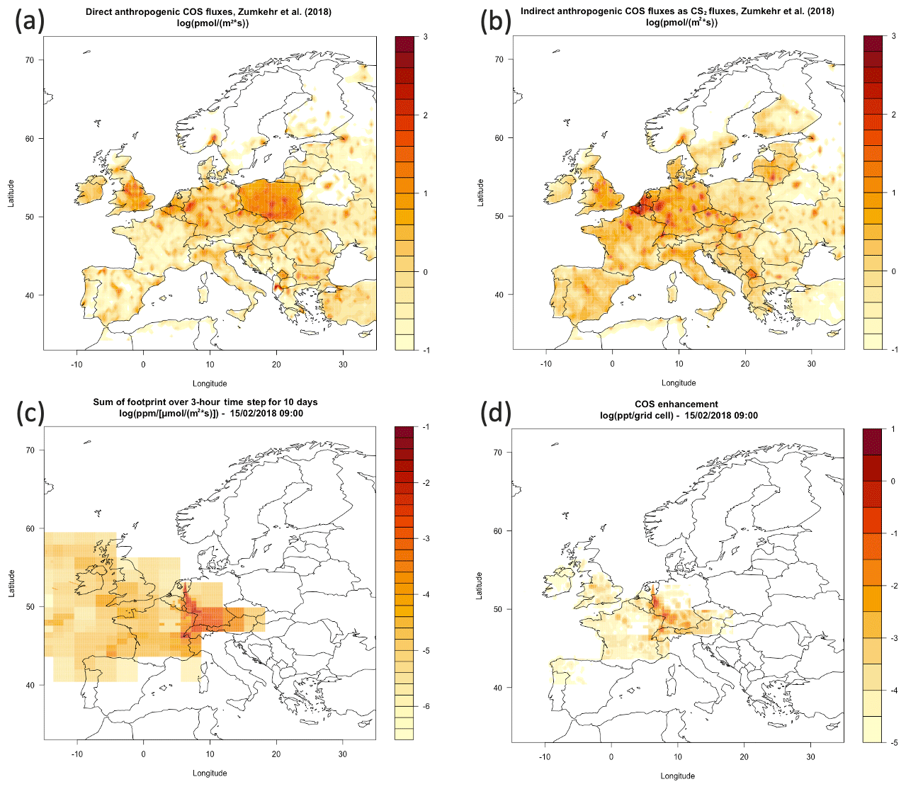
Figure 2 Reported in logarithmic scales: (a) and (b) show the localized COS and CS₂ sources according to Zumkehr et al. (2018); (c) shows an example of localized footprint values resulting from the STILT model simulations, summed over 10 d before the starting time step (15 February 2018, 09:00 CET (UTC+1)); and (d) the modeled enhancement resulting from the product of footprint and fluxes (see Sect. 2.4), identifying the sources influencing Lutjewad in the Ruhr area (the ranges of these scales were adjusted for clarity purposes).

Ultimately, the total COS molar fraction simulation of each time step can be calculated using Eq. (3), over 3 h time steps, for the months of January and February 2018:

$$\begin{array}{}\text{(3)}& C_{\mathrm{COS}}=B_{\mathrm{COS}}+\mathrm{\Delta }\mathrm{COS},\end{array}$$

where C_COS is the total COS molar fraction, B_COS the COS background and ΔCOS the COS enhancement (or depletion, for ΔCOS_bio) associated with fluxes calculated with Eq. (2).

In addition, CO₂ molar fractions were simulated using the STILT footprint tool implemented at ICOS Carbon Portal (Karstens et al., 2022). This tool combines STILT simulations with anthropogenic CO₂ emissions categorized by sector from the EDGAR v4.3 inventory (Janssens-Maenhout et al., 2017) and biospheric CO₂ fluxes from the Vegetation Photosynthesis and Respiration Model (VPRM) (Mahadevan et al., 2008).

3 Results

3.1 Estimate of nighttime COS and CO₂ fluxes

Figure 3 shows the nighttime fluxes of COS and CO₂ in Lutjewad based on the radon-tracer method. Most of the derived COS fluxes are negative, implying COS sinks at the surface. Occasionally, there are positive fluxes, which coincide with periods in which we observe COS spikes after plowing (see Kooijmans, 2018). The median nighttime COS flux is $-\mathrm{3.0}\pm \mathrm{2.6}$ pmol m⁻² s⁻¹ (excluding the positive fluxes), with $-\mathrm{2.9}\pm \mathrm{2.2}$ pmol m⁻² s⁻¹ from August to November 2015 and $-\mathrm{7.2}\pm \mathrm{2.8}$ in April 2015. The average SiB4 COS nighttime (21:00–06:00 CET (UTC+1)) flux was retrieved for Lutjewad (53.4^∘ N, 6.3^∘ E) for January and February 2018 and was estimated to be $-\mathrm{2.1}\pm \mathrm{0.2}$ pmol m⁻² s⁻¹. The nights with COS emissions have an average COS flux of $+\mathrm{3.5}\pm \mathrm{2.1}$ pmol m⁻² s⁻¹. Nighttime CO₂ fluxes decrease from August to December, then increase in January and reach their highest levels in April (note that CO₂ fluxes from May–July are not available).

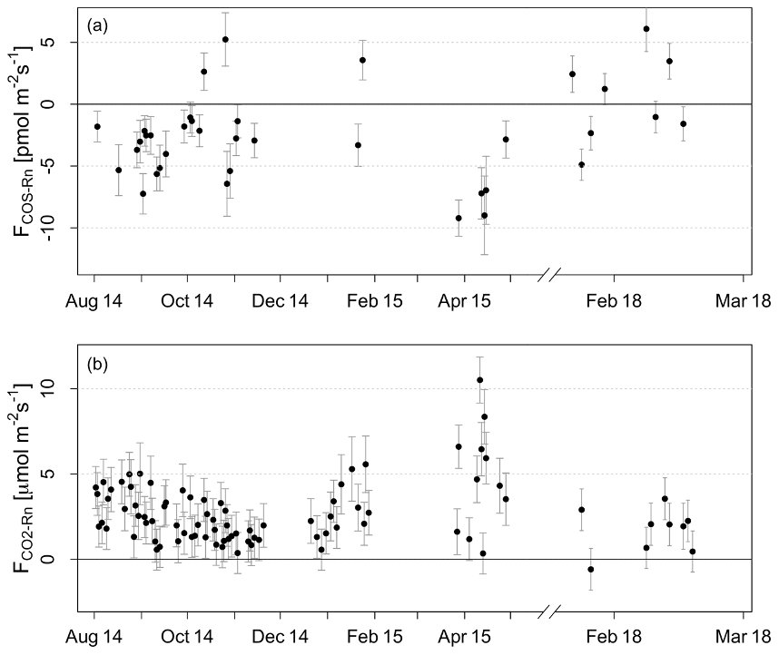
Figure 3 Nighttime fluxes of COS (a) and CO₂ (b) in Lutjewad based on the radon-tracer method. Note that the x axis jumps from April 2015 to February 2018.

3.2 Modeled and observed COS and CO₂ mole fraction

The period of January and February 2018 is characterized by a few episodes of increased COS mole fractions that sometimes last for a few hours but also extend to a few days (Fig. 4). This period was characterized by cold weather (air temperature <0 ^∘C), which allowed plowing activities with heavy machinery in the agricultural fields surrounding the station. At 60 m, we observed COS elevations on the order of hundreds of ppt above the background mole fraction over a period of a few days. CO₂ and CO (the latter is not shown in Fig. 4) molar fractions are also elevated when COS is higher. CO₂ and CO mole fractions are strongly correlated in this period (R²=0.94), and the ratio of CO to CO₂ elevations in this period is 5.3 ppb ppm⁻¹. COS mole fractions are not as strongly correlated with CO₂ and CO (R²=0.50 and 0.48, respectively).

The observations of COS and CO₂ in the period of January and February 2018 were further investigated, using the simulations described in Sect. 2.4. Figures 4 and 5 show the comparison between the modeled results and the measurements in Lutjewad for January and February 2018. The model generally reproduces the measurement trend well for both species. For CO₂, the average difference between measurements and modeled values was 3.6 ± 5.4 ppm (Fig. 5b). The model captures the CO₂ enhancements on 22–28 January (Period 1, R²=0.74), 30–31 January (Period 2, R²=0.88), 5–11 February (Period 3, R²=0.61) and 12–15 February (Period 4, R²=0.82), although generally it slightly underestimates the total molar fraction (see Figs. 4 and 5 as well as the regression analysis between modeled results and measurements, reported in Figs. S4 and S5 in Sect. S2 of the Supplement). Figure 6 shows the contribution of background, biosphere and anthropogenic emissions to the final results for both gases. Anthropogenic emissions represented the biggest contributors to the deviations from the background for both gas species. As expected, the biospheric influence results in emissions for CO₂ due to the respiration process which dominates plant behavior in winter. In contrast, the biospheric contribution to COS molar fraction results in depletion of this gas species, which can be attributed to soil uptake. Four periods when either COS or CO₂ showed significant enhancements compared to the background were selected within the investigated time frame. According to the model, most of the enhancements can be attributed to industry in the Ruhr area (Period 4) and the Antwerp–Rotterdam region (Periods 1 and 2 and last part of Period 3). Interestingly, the Ruhr area is also responsible for the overestimation occurring on 19 February for both species. For Periods 1, 2 and 4 the model estimates roughly between 51 % and 68 % of the measured CO₂ enhancements. On the other hand, Period 3 is related to the lowest R² value and to the highest underestimation, simulating just around 32 % of the measured enhancements (see Figs. 4b, 5b). This is the only period related to eastern footprints in the selected time frame.

With regard to COS, it is clear that the model generally shows a slight overestimation of its molar fraction, with an average difference between measurements and modeled values of −4.5 ± 26.9 ppt (Fig. 5a). The model is generally less accurate in reproducing COS mole fractions when compared to its CO₂ performance. However, the model still captures 61 % of the enhancements of Period 4 (R²=0.70), which the STILT model attributes to the Ruhr area. Moreover, the model captures singular peaks related to the Ruhr area's emissions in Period 1 (over the whole period, R²=0.23). Furthermore, it reproduces the trends of the enhancements in the second part of Period 3 (Fig. 4a, 8–11 February). This period is related to a mixed southern and eastern footprint, which ascribes this share of enhancements to the Antwerp–Rotterdam area and to paper production locations in northern Germany (an example is shown in Fig. S6). Nonetheless, severe underestimations occur persistently between 7–10 February and as singular events around 6 and 17 February (Fig. 4a). The largest underestimation of COS reaches around 254 ppt on 7 February (Fig. 5a). As stated earlier in the text, Period 3 and 17 February, unlike most of the other periods, are characterized by eastern-footprint outputs, followed by high footprint values close to the Lutjewad area. Altogether, this suggests that the emissions of both COS and CO₂ east of Lutjewad may be underestimated. Noticeably, the highest CO₂ underestimations, occurring between 9 and 10 February and reaching up to 26.9 ppm (Fig. 5b), are mostly related to southern influences but still show high influences from the Lutjewad surroundings.

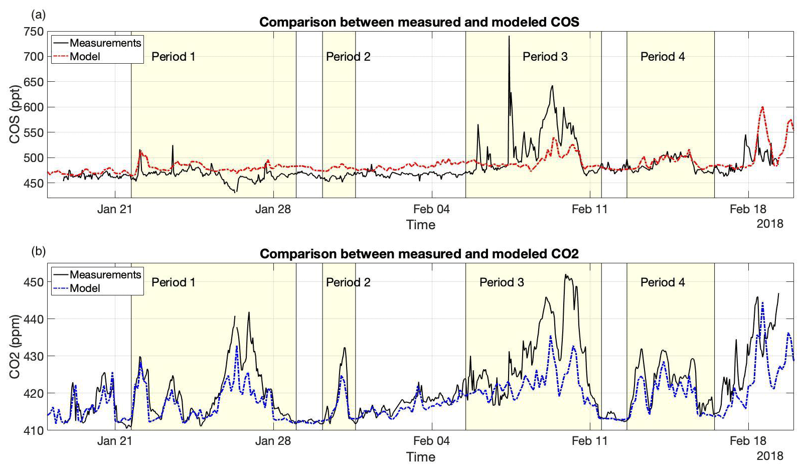
Figure 4 Modeled and observed mole fractions of (a) COS and (b) CO₂ in Lutjewad (60 m a.g.l.) in January and February 2018 (the time format on the x axes is “month day”). The periods of interest in this time frame are highlighted in yellow: during these time intervals, CO₂ and/or COS enhancements were measured.

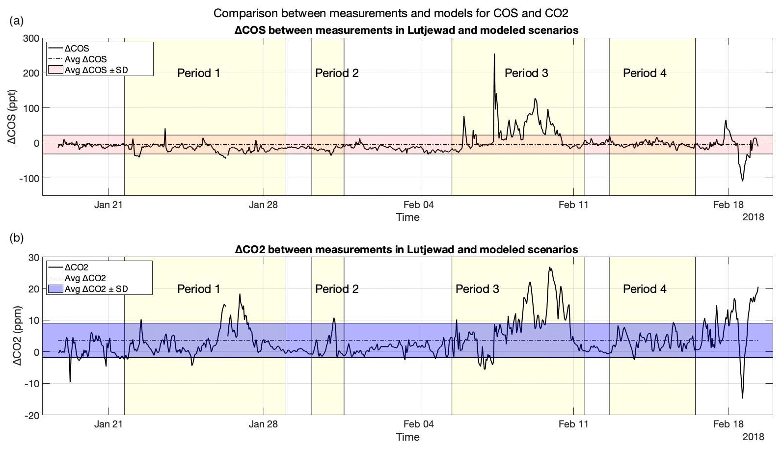
Figure 5 Difference between modeled and observed (a) COS and (b) CO₂ mole fractions. The red- and blue-shaded areas include the values lying between the average difference between measurements and models ± the standard deviation of this difference.

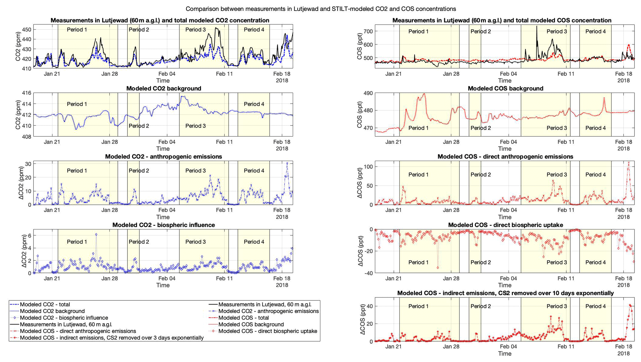
Figure 6 Mole fractions of CO₂ and COS, showing the contributions of background, biosphere and anthropogenic emissions. The top plots show the difference between modeled results and measurements for both gases. The indirect emissions of COS in this figure were computed assuming a 10 d exponential conversion of CS₂ to COS.

3.3 Discrete samples and in situ measurements

During the sampling activities using flasks and a mobile van, described in Sect. 2.2.2, COS sources were identified. In particular, emissions were found at the Suiker Unie facilities (53.2^∘ N, 6.5^∘ E), at the Attero facilities (53.2^∘ N, 6.6^∘ E), and at coal- and aluminum-related industries in Eemshaven (53.4^∘ N, 6.8^∘ E) and in the Delfzijl–Farmsum area (53.3^∘ N, 6.9^∘ E) (see Fig. 1). Given the southeasterly wind direction during sampling, it was not possible to separate the contribution of each company in Farmsum to the measured mole fractions. Therefore, these results will be reported by the name of the industrial facilities: ChemiePark. The only company that could be easily isolated in the area was ESD-SIC (53.3^∘ N, 7.0^∘ E), a silicon carbide producer (see Fig. 7a, b). This company is known to be related to occasional explosive events (Dagblad van het Noorden, 2018; Provincie Groningen, 2018a; The Northern Times, 2018), which will be discussed later in the text. Discrete sampling was performed in Eemshaven, where industries and energy plants based on fossil fuels can be found, and at the Attero facilities for waste treatment and biogas production. The results of these samples are presented in Tables S1 and S2 of the Supplement. Among these results, COS enhancements between tens of ppt and about 100 ppt were measured at the waste disposal site and at the biodigesters of Attero. Suiker Unie facilities also produce biogas from the sugar treatment leftovers, and at this site COS mole fractions went up to 1.8 ppb, almost 1.3 ppb above the background values. These findings are of particular interest, as will be described in Sect. 4.1. In situ measurements from a mobile van were performed at the fields near the Lutjewad station at the end of October 2019 while the area was being plowed. On this occasion, no COS enhancements were detected from plowing activities. The results of continuous measurements showing COS enhancements are reported in Table 3. The fluxes for the in situ measurements were calculated with a Gaussian dispersion model after Csanady et al. (1973), using COS mole fractions, distance from the source and wind speed. The errors were estimated performing a Monte Carlo simulation, similarly to Bakkaloglu et al. (2021). The COS enhancements from the background were chosen from a uniform distribution within the observed enhancement range. Distance from the source and wind speed were selected from a normal distribution centered at the estimated distance and average wind speed. The estimated wind speed determined the stability class for the Gaussian dispersion model for each specific run of the Monte Carlo simulation. For some of these sources, such as Suiker Unie, biodigesters and industries in Farmsum, co-emissions of COS with CO, CO₂, CH₄ and N₂O were occasionally measured. As reported in Table 3, the highest enhancements were measured at the ChemiePark, and the related fluxes were consequently estimated in the range of 9369 ± 8582 kg(COS) a⁻¹.

Table 3 Summary of COS fluxes obtained with in situ measurements combined with Monte Carlo simulations. COS fluxes are reported as both COS and S emission rates. Suiker Unie is a seasonal factory that runs for about 5 months; thus, the reported yearly emissions should be considered just a tool to compare the magnitude of different sources of COS when the companies are active.

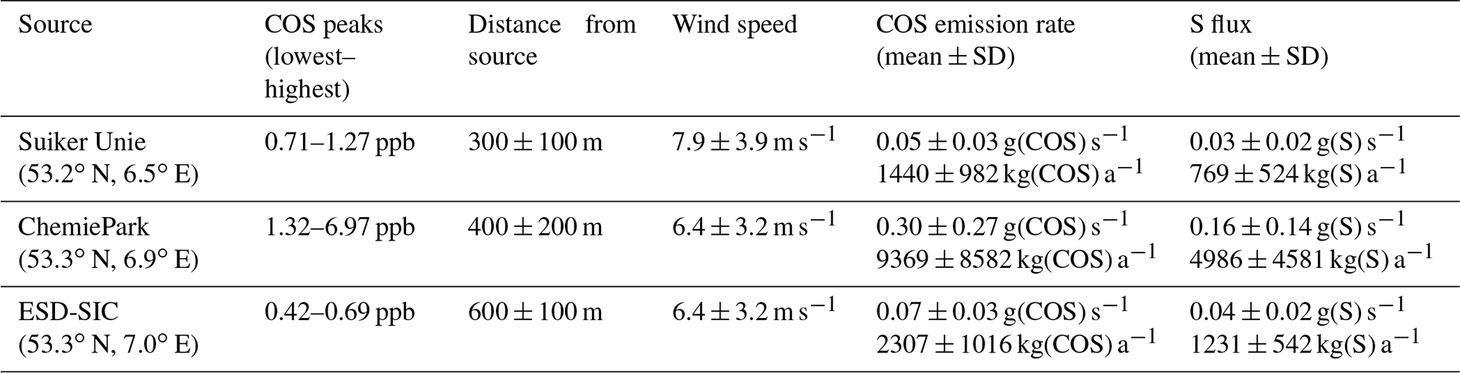
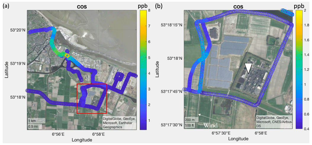
Figure 7 (a) Results of the COS in situ observations in the Farmsum site. The ESD-SIC area is highlighted with a red square in (a) and shown alone in (b). The emissions at ESD-SIC were strongly correlated with CO and CH₄.

3.3.1 Influence of observed local sources

As described in Sect. 3.2, mismatches were found between measurements at the Lutjewad station and the respective modeled results. Often, these mismatches were related to the high influences of areas east of Lutjewad and in the station's surroundings, in particular the areas of Groningen and northeast Germany. Therefore, we added the fluxes in Table 3 to the available anthropogenic database described in Sect. 2.4 to check whether they could explain the gap described in Sect. 3.2. After the implementation of the local fluxes at their respective coordinates, all belonging to the Groningen area, these sources accounted for a total of 93.7 pmol m⁻² s⁻¹. Consequently, COS mole fractions were recalculated using the model described in Sect. 2.4. The resulting time series was then compared with the results described in Sect. 3.2, as shown in Fig. 8. The additional sources, according to the estimated fluxes, would only have a marginal effect on the final results. Nonetheless, the highest increases occur during the same time as periods when the model underestimates the results the most (5–10 February and, to a smaller degree, 17–19 February), signalling a higher local influence at such occasions.

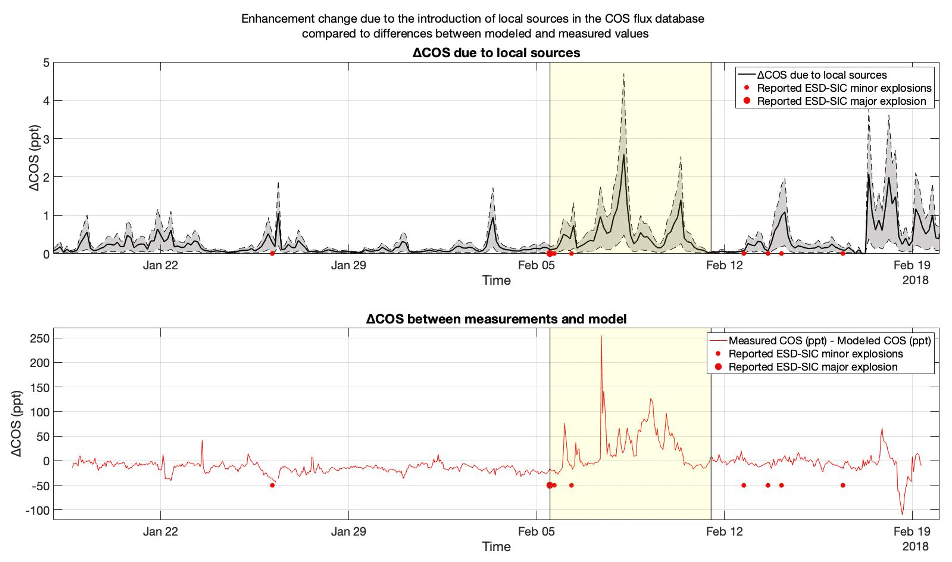
Figure 8 COS increase in the results after the introduction of local sources in the model, reported as mean contribution (black line) ± the relative standard deviation (grey area). The period when the highest underestimations occur, which coincides with the highest contributions of local sources to the final results, is highlighted in yellow. The red dots show explosive events occurring at ESD-SIC, which are discussed in the text.

To understand how large local emissions would have to be to explain this gap, the highest enhancement from the background (261.7 ppt, on 7 February at 09:00 CET (UTC+1)) was divided by the sum of local footprints between Lutjewad and the identified sources (52.9–53.4^∘ N, 6.3–7^∘ E) associated with this date. This resulted in an estimated local flux of 148.3 pmol m⁻² s⁻¹. Hypothesizing an even distribution of the sources presented in Table 3 over the same area, local emissions would result in a flux of 2.4 pmol m⁻² s⁻¹. Therefore, the estimated local flux needed to justify the highest measured enhancement in Lutjewad is roughly 2 orders of magnitude higher than the one resulting from the measurements in Table 3. This suggests this peak could only be related to a peculiar event, as will be discussed later in Sect. 4.1.1.

4 Discussion

4.1 Anthropogenic sources of COS

The COS enhancements measured in Lutjewad between 2014 and 2018 were firstly attributed to either plowing activities or other anthropogenic emitters. As reported in Sect. 3.3, no emissions were found from plowing activities during this study. However, the measurements for plowing activities were rather limited, and, knowing that rapeseed was grown in some fields in the province of Groningen, it is still possible that a fertilizer based on rapeseed byproducts (Belviso et al., 2022a) or the soil acts as a COS source occasionally, depending on soil moisture, temperature, composition and use (Kaisermann et al., 2018; Katayama et al., 1992; Kitz et al., 2017; Maseyk et al., 2014; Whelan et al., 2018). Overall, it remains unclear if plowing contributed to the measured COS enhancements.

The results presented in Sect. 3.3 demonstrate the presence of local sources of COS in the province of Groningen. Unfortunately, it was not possible to link the emissions to specific production rates or resources consumption of the observed companies due to lack of information about these parameters. Nonetheless, it is notable that COS emissions were measured from biodigesters, present at the Attero and at the Suiker Unie facilities. Biodigesters are currently not included as sources in the available databases (Campbell et al., 2015; Zumkehr et al., 2018), but the presence of COS has been reported in different food products, such as cheese and cabbage (Aston and Douglas, 1981; Maarse, 1991). Therefore, the role of organic waste as a source of COS could be potentially significant on a global scale and should be further investigated.

According to the footprints obtained using the STILT model, some COS enhancements can be ascribed to known European industrial areas. These include the Ruhr area (Germany); Antwerp (Belgium); Rotterdam–Amsterdam (Netherlands); and, less frequently, northeast Germany, eastern Europe or the United Kingdom. The Ruhr area, in particular, seems to be almost fully accountable for the enhancements measured between 14–15 February (Figs. 4, 5, 6). However, the mismatch between 5 and 10 February could not be ascribed to air transport from known sources. In this period, STILT simulations found eastern footprints showing high influences of Lutjewad's surroundings. The influence of local sources is small according to the available measurements. Nonetheless, as described in the following paragraph, specific exceptional local events could explain the unusually high COS mole fractions measured during this time interval.

Explosions at ESD-SIC

Among the measured local COS sources, ESD-SIC deserves a particular focus. The company produces silicon carbide (SiC) using the Acheson process, which involves high-temperature furnaces where petroleum coke and silica (sand, SiO₂) can react, producing SiC and CO. The reaction between petroleum coke and sand produces low-calorific process gas which contains around 1 % sulfur-containing compounds (ESD-SIC, 2022). This gas then undergoes a desulfurization process which removes around 90 % of the sulfur compounds (ESD-SIC, 2022). Coke-derived gases have been reported to contain sulfur compounds, including COS (Ferm, 1957). Zeng et al. (2021) also report significant quantities of CS₂ and COS being produced by the thermal oxidative reaction of sulfur-containing compounds in the presence of hydrocarbons. Together with what ESD-SIC explains on their website, this could explain the observed COS enhancements reported in Table 3. Moreover, this company has been reported to cause a nuisance on several occasions with smell or, more noticeably, with explosions (Provincie Groningen, 2018a, b). Local newspapers have broadly covered these occurrences: already on 13 January 2015 an explosion covered the villages of Meedhuizen and Tjuchem (situated about 5 km south-southwest of ESD-SIC) in SiC soot (RTVNoord, 2015). On those dates, no COS enhancements were observed in Lutjewad. However, the footprints calculated for that period suggest that the measured air originated southwest of the station (ICOS, 2022). Later, frequent explosions occurred in January and February 2018 (Dagblad van het Noorden, 2018; Provincie Groningen, 2018a, b; RTVNoord, 2018; The Northern Times, 2018). Among these, a particularly severe explosion happened on 5 February 2018 at 11:55 CET (UTC+1), which was followed by two smaller explosions, the same day at 15:54 and on 6 February at 07:15 (Provincie Groningen, 2018a). As explained in Sect. 3.3, the highest COS and CO₂ enhancements in Lutjewad, severely underestimated for both species by the modeled results, were found between 5 and 10 February. The footprints related to these dates indicate eastern origins for the measured air. This finds further confirmation in local newspapers articles which, again, describe easterly winds and soot-related problems in villages west of ESD-SIC following the explosions (Dagblad van het Noorden, 2018; RTVNoord, 2018). The measurements for ESD-SIC (Table 3) on a non-explosion occasion and their implementation in the model (Fig. 8) would not justify the differences between the modeled results and the measurements. Nonetheless, given the results and the information available, the occurrence of these explosions during easterly wind conditions could be the reason behind the enhancements measured in Lutjewad between 2014 and 2018. However, it is good to mention that the model resolution might have not been high enough to reproduce the dispersion of emissions in such a limited zone. Moreover, it is possible that other sources could be present near Lutjewad or in general in the areas influencing the observations at the tower. Furthermore, the vertical mixing parameter of the model may have been too fast to correctly simulate the plume transport in such a limited area with stable night conditions. Also, possible indirect emissions of CS₂ were not considered in this simulation. In other words, a model with a higher resolution and/or a more detailed database would probably produce a different and more accurate estimate for the missing source in the area. Therefore, the missing source of 148.3 pmol m⁻² s⁻¹ presented in Sect. 3.3.1 should be considered just a rough estimate.

4.2 COS and GPP

The results presented in Sect. 3.2 and 3.3 underline the relevance of assessing a thorough regional COS budget in the context of using this gas as a tracer for GPP. From this study, it is clear that both the background molar fraction and the enhancements measured in Lutjewad are influenced by anthropogenic sources. In fact, excursions of the COS molar fraction can be ascribed to both local sources and sources located hundreds of kilometers from the station, such as the Ruhr area in Germany. A poor assessment of COS sources may lead to biased findings with regard to COS flux estimations, which would therefore mislead the GPP evaluation. With regard to the observed COS enhancements, inverse transport models provide a tool to prevent inaccurate interpretations or at least to allow a preliminary assessment of possible biases due to the origin of the analyzed air.

5 Conclusions

We have inferred the regional sources and sinks of COS using continuous in situ mole fraction profile measurements of COS along the 60 m tall Lutjewad tower (1 m a.s.l.; 53^∘24^′ N, 6^∘21^′ E) in the Netherlands. To identify potential sources that caused the observed enhancements of COS mole fractions at Lutjewad, we have made both discrete flask samples and in situ measurements in the province of Groningen from a mobile van using a quantum cascade laser spectrometer (QCLS). We detected lower COS mole fractions from inland, which are likely driven by vegetation and soil uptake, and found no indications that the mudflats and salt marshes at the coast are a net sink or a net source. The nighttime COS fluxes were determined to be $-\mathrm{3.0}\pm \mathrm{2.6}$ pmol m⁻² s⁻¹ using the radon-tracer correlation approach. Furthermore, local sources of COS were identified in the province of Groningen. Among these, emissions were measured at biodigesters and facilities related to organic waste processing. Biodigesters and organic waste are currently not included in emission databases of COS. However, the COS emissions have not been linked to specific process capacities or resource consumption, which currently limits the upscaling of these newly found sources for modeling purposes. The same issues apply to agricultural soils, which could not be fully proven as a COS source or sink.

We simulated both COS and CO₂ concentrations at the Lutjewad station using STILT and found that part of the observed COS enhancements can be explained by known industrial areas in Europe, such as the Ruhr area or the harbors of Antwerp and Rotterdam. Nonetheless, strong emissions during explosions occurring at ESD-SIC, a silicon carbide producer in the province of Groningen, could potentially explain large COS enhancements that were associated with easterly wind conditions. Our study demonstrates that the influence of local to regional anthropogenic sources should be considered when using COS measurements as a tracer for GPP, especially for atmospheric measurements that are close to urban areas. This approach, combining COS stationary measurements, mobile measurements and models, could be applied in other existing measurement locations. It could allow a broader assessment of local anthropogenic influences to prevent biases in COS budget and seasonality estimates.