Alkalinity biases in CMIP6 Earth system models and implications for simulated CO₂ drawdown via artificial alkalinity enhancement

The partitioning of CO₂ between atmosphere and ocean depends to a large degree not only on the amount of dissolved inorganic carbon (DIC) but also on alkalinity in the surface ocean. That is also why ocean alkalinity enhancement (OAE) is discussed as one potential approach in the context of negative emission technologies. Although alkalinity is thus an important variable of the marine carbonate system, little knowledge exists on how its representation in models compares with measurements. We evaluated the large-scale alkalinity distribution in 14 CMIP6 Earth system models (ESMs) against the observational data set GLODAPv2 and show that most models, as well as the multi-model mean, underestimate alkalinity at the surface and in the upper ocean and overestimate it in the deeper ocean. The decomposition of the global mean alkalinity biases into contributions from (i) physical processes (preformed alkalinity), which include the physical redistribution of biased alkalinity originating from the soft tissue and carbonates pumps; (ii) remineralization; and (iii) carbonate formation and dissolution showed that the bias stemming from the physical redistribution of alkalinity is dominant. However, below the upper few hundred meters the bias from carbonate dissolution can gain similar importance to physical biases, while the contribution from remineralization processes is negligible. This highlights the critical need for better understanding and quantification of processes driving calcium carbonate dissolution in microenvironments above the saturation horizons and implementation of these processes into biogeochemical models.

For the application of the models to assess the potential of OAE to increase ocean carbon uptake, a back-of-the-envelope calculation was conducted with each model's global mean surface alkalinity, DIC, and partial pressure of CO₂ in seawater (pCO₂) as input parameters. We evaluate the following two metrics: (1) the initial pCO₂ reduction at the surface ocean after alkalinity addition and (2) the uptake efficiency (ηCO₂) after air–sea equilibration is reached. The relative biases of alkalinity versus DIC at the surface affect the Revelle factor and therefore the initial pCO₂ reduction after alkalinity addition. The global mean surface alkalinity bias relative to GLODAPv2 in the different models ranges from −85 mmol m⁻³ (−3.6 %) to +50 mmol m⁻³ (+2.1 %) (mean: −25 mmol m⁻³ or −1.1 %). For DIC the relative bias ranges from −55 mmol m⁻³ (−2.6 %) to 53 mmol m⁻³ (+2.5 %) (mean: −13 mmol m⁻³ or −0.6 %). All but two of the CMIP6 models evaluated here overestimate the Revelle factor at the surface by up to 3.4 % and thus overestimate the initial pCO₂ reduction after alkalinity addition by up to 13 %. The uptake efficiency, ηCO₂, then takes into account that a higher Revelle factor and a higher initial pCO₂ reduction after alkalinity addition and equilibration mostly compensate for each other, meaning that resulting DIC differences in the models are small (−0.1 % to 1.1 %). The overestimation of the initial pCO₂ reduction has to be taken into account when reporting on efficiencies of ocean alkalinity enhancement experiments using CMIP6 models, especially as long as the CO₂ equilibrium is not reached.

1 Introduction

Since preindustrial times the ocean has taken up about a quarter of the anthropogenic CO₂ emitted into the atmosphere (Friedlingstein et al., 2022). The exact amount of ocean CO₂ uptake is determined by the surface ocean carbonate system, which can be largely described by the amount of dissolved inorganic carbon (DIC) and total alkalinity (TA) in the surface ocean (Zeebe and Wolf-Gladrow, 2001). Total alkalinity is a measure of the excess of bases (proton acceptors) over acids (proton donors) and plays a central role in determining the partitioning of the DIC pool into its three chemical components, aqueous CO₂ and bicarbonate (HCO${}_{\mathrm{3}}^{-}$) and carbonate (CO${}_{\mathrm{3}}^{\mathrm{2}-}$) ions. Aqueous CO₂ is the only of the three marine carbonate species that can exchange with the atmosphere. Once in the ocean, most of the additional CO₂ taken up is converted into the two other carbonate species. By changing the chemical equilibria between the carbonate species, the ocean carbon uptake leads to ocean acidification with a decrease in pH. This change in the chemical equilibria also reduces the seawater buffer capacity, i.e., the ability of seawater to resist a change in its carbonate chemistry. The Revelle factor, as a measure of this buffer capacity, is the sensitivity of relative pCO₂ (partial pressure of CO₂ in seawater) change to relative changes in DIC and depends both on DIC and TA. A low Revelle factor indicates a high buffering capacity and vice versa (Revelle and Suess, 1957; Middelburg et al., 2020). The lower the Revelle factor, the more DIC occurs as CO${}_{\mathrm{3}}^{\mathrm{2}-}$ and pCO₂ levels in the ocean are lower. This allows the ocean to take up more CO₂, which in turn also lowers atmospheric pCO₂ (Egleston et al., 2010). Overall, the buffer capacity implies that the resulting change in pH and CO₂ from the same process, e.g., carbonate dissolution, differs depending on the background conditions in TA and DIC (Middleburg et al., 2020). Any changes in pH and CO₂ would be smaller in low-sensitivity or well-buffered seawater with a high TA : DIC ratio (low Revelle factor). That is why it is important that Earth system models (ESMs) simulate reasonable initial states of TA and DIC when they are used to quantify the potential CO₂ uptake of the ocean.

In 2015, the “Paris Agreement” was adopted by 196 governments at the Conference of the Parties 21 (COP21). Its goal is to restrict human-induced global warming to well below 2 ^∘C, preferably to 1.5 ^∘C, compared to preindustrial levels. To accomplish this goal, the signing countries aim to reach peak emissions as quickly as possible and to achieve carbon neutrality by the mid-21st century. This goal is likely not achievable through carbon emission reductions alone according to socio-economic scenario simulations with integrated assessment models (Rogelj et al., 2018). The IPCC Special Report on Global Warming of 1.5 ^∘C states that all (most) projected pathways that limit warming to 1.5 ^∘C (2 ^∘C) also require use of carbon dioxide removal (CDR) or negative emission technologies (NETs) on the order of 100–1000 Gt CO₂ over the 21st century (Rogelj et al., 2018). Existing and potential CDR measures are afforestation and reforestation, land restoration and soil carbon sequestration, bioenergy with carbon capture and storage (BECCS), direct air carbon capture and storage (DACCS), enhanced weathering, and ocean alkalinization (Gattuso et al., 2018; de Coninck et al., 2018; National Academies of Sciences, Engineering, and Medicine, 2019, 2022). So far, much research has focused on land-based CDR measures, and it has become clear that it would be extremely difficult to limit global warming to the agreed level with land-based NETs alone (Fuss et al., 2018; Lawrence et al., 2018; Smith et al., 2016).

Less is known about ocean-based NETs, although some of them appear promising, especially with respect to the potential scale of application (Gattuso et al., 2018; GESAMP, 2019). One promising pathway could be ocean alkalinity enhancement (OAE; Köhler et al., 2013; Renforth and Henderson, 2017). This method is an accelerated version of the natural process of silicate weathering, where alkaline minerals can be mined and crushed (e.g., olivine) or created (e.g., lime) and added to the surface ocean. Alternatively, alkaline solutions from electrochemical weathering can be added. In both scenarios, the alkalinity of the upper ocean is increased and with it the carbon storage capacity of seawater, which leads to an increased uptake of CO₂ from the atmosphere. Aside from lab experiments (Hartmann et al., 2023) and first results from microcosm experiments (Ferderer et al., 2022), these OAE applications are untested at larger scales, meaning that simulations with state-of-the-art ESMs are essential for assessing the efficiency and biogeochemical implications of ocean alkalinization. Previous model experiments have provided first estimates of the efficiency for idealized experiment setups (e.g., Ilyina et al., 2013; Köhler et al., 2013; Keller et al., 2014; Hauck et al., 2016; González and Ilyina, 2016; Lenton et al., 2018; Burt et al., 2021). Although these modeling studies have suggested that OAE may be a viable method to help reduce atmospheric CO₂, the results are difficult to compare due to different experimental designs. Another caveat is that previous estimates of OAE efficiency and side effects were based on single-model experiments and did not include a thorough assessment of simulated alkalinity and model dependence of the results. Now, more and more projects are underway or in planning that seek to apply more realistic scenarios for OAE, e.g., in regional OAE applications (Butenschön et al., 2021; Wang et al., 2023) or coastal applications (Feng et al., 2017; He and Tyka, 2023), which is why a model evaluation is even more important. Furthermore, the development of standards for monitoring, reporting, and verification (MRV) methods for real-world OAE applications is currently underway and it is becoming clear that numerical simulations are required to fulfill these MRV requirements because of the complexity of the carbonate system and the insufficient maturity of observational sensors (Ho et al., 2023; Bach et al., 2023). Therefore, the continuous development of suitable, carefully validated models is a critical part of this effort (Ho et al., 2023).

There have been a number of studies that evaluate the simulation of ocean biogeochemical parameters in state-of-the-art ESMs that contributed to CMIP6, the sixth phase of the Coupled Model Intercomparison Project (Eyring et al., 2016), but did not include the evaluation of alkalinity (Séférian et al., 2020; Tagliabue et al., 2021; Kwiatkowski et al., 2020) or if they did then only with one global score number (Terhaar et al., 2022; Fu et al., 2022). The recent study by Planchat et al. (2023) assessed simulated alkalinity and parameters related to the carbonate pump in CMIP6 models and their predecessor CMIP5 versions. They report an improvement in the representation of alkalinity and the carbonate pump in CMIP6 versus CMIP5. While some models did increase in complexity, they find that potential effects of future ocean changes (e.g., ocean acidification) are not well constrained in many models.

Here, we present further analyses of biases in alkalinity and DIC in CMIP6 models. We show how those biases can be attributed to the ocean's physical, soft-tissue, or carbonate counter pump following Koeve et al. (2014). Furthermore, we provide an estimate of each model's carbonate system sensitivity to OAE depending on their alkalinity and DIC bias in historical simulations.

2 Methods

2.1 CMIP6 models and observational data products

Our evaluation includes 14 ESMs with ocean biogeochemistry modules from 10 modeling centers that contributed to CMIP6 and that provided most of the following variables: “dissic” (DIC [mol m⁻³]), “no3” (nitrate concentration [mol m⁻³]), “o2” (dissolved oxygen concentration [mol m⁻³]), “ph” (seawater pH on total scale), “po4” (phosphate concentration [mol m⁻³]), “so” (salinity (S) [g kg⁻¹]), “talk” (TA [mol m⁻³]), and “thetao” (potential temperature [^∘C]), see Table 1.

Table 1 Overview of CMIP6 models considered in this study listing the climate model name and description paper, the model ocean component, the model biogeochemistry component, horizontal grid resolution, number of vertical levels, the ensemble member considered, and the data reference

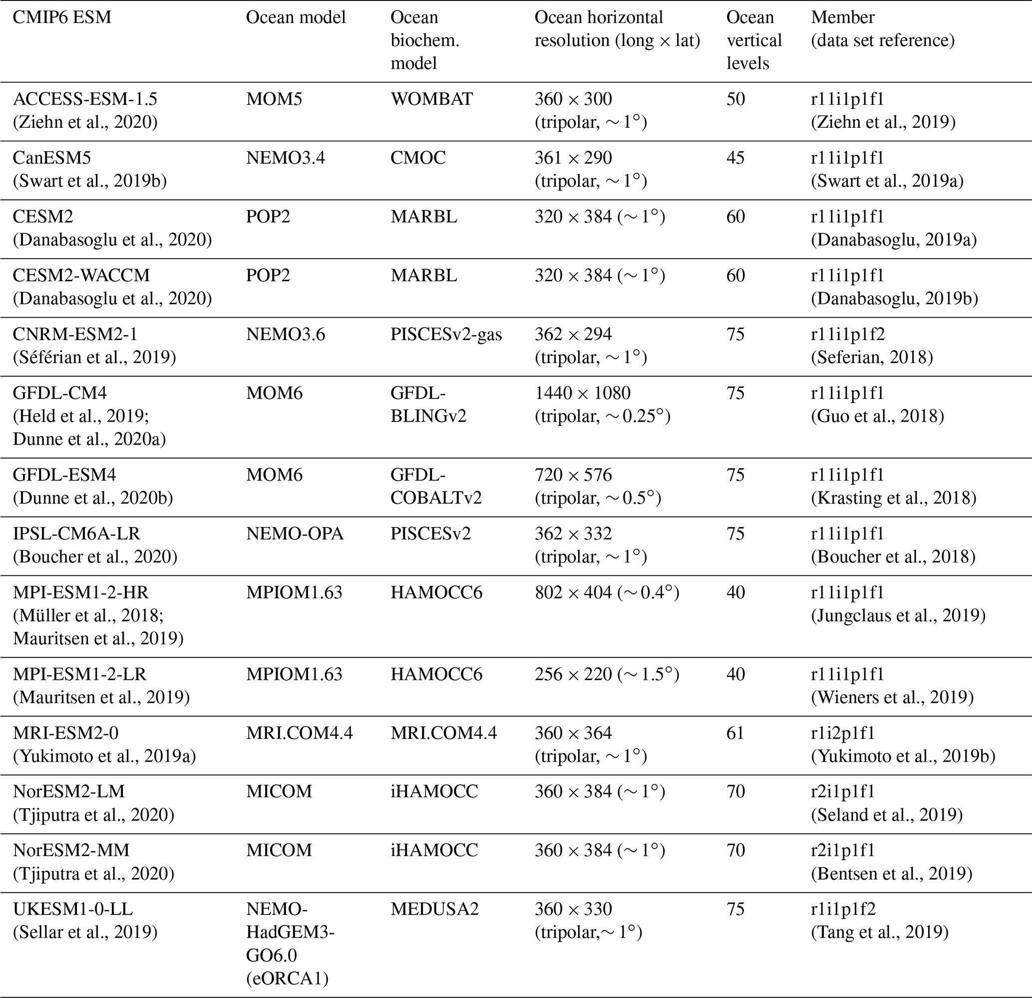
For the 14 CMIP6 ESMs, monthly data from one ensemble member (see Table 1) of the historical simulation were downloaded from the CMIP6 archive (https://esgf-data.dkrz.de, last access: 8 March 2022), post-processed, and regridded with bilinear remapping onto a common 1^∘ × 1^∘ grid using Climate Data Operators (CDO, Schulzweida, 2022). TA is often normalized (TA_n) with salinity to exclude the freshwater effect in the alkalinity assessment (Millero et al., 1998; Fry et al., 2015). Salinity normalization of alkalinity was achieved by using a reference salinity of 35 g kg⁻¹. Grid points with a salinity smaller than 10 were masked to avoid very high TA_n values, e.g., from the Baltic Sea:

$$\begin{array}{}\text{(1)}& {\mathrm{TA}}_{\mathrm{n}}={\displaystyle \frac{\mathrm{TA}}{S}}\times \mathrm{35},\end{array}$$

with S being the grid point salinity. The present-day (1995–2014) model climatologies from the historical simulations are evaluated against gridded observational products: (i) TA, DIC, and pH from the GLODAPv2.2016b Mapped Climatology (in the following GLODAP, Lauvset et al., 2016); (ii) oxygen and nutrients from the World Ocean Atlas 2018 data set (WOA, Garcia et al., 2019) and GLODAP (not shown); and (iii) salinity and temperature from the Polar science center Hydrographic Climatology (PHC3.0, Steele et al., 2001) and WOA (not shown). For the evaluation of global mean vertical profiles, the model data are interpolated onto the same 33 vertical levels used in the GLODAP climatology. For the purpose of model assessment, the GLODAP TA and DIC data are converted from units of µmol kg⁻¹ to mmol m⁻³ using the potential density computed from GLODAP salinity and temperature data.

2.2 Analysis of the vertical distribution of total alkalinity – the TA^* method

In order to better understand the vertical distribution of modeled alkalinity compared to the observed one, we follow the “TA^* method” as described by Koeve et al. (2014). This method aims to separate the effects of biogeochemical processes and ocean circulation on the distribution of TA. To achieve this, TA is separated into three components: preformed TA (TA⁰), TA decrease from remineralization of organic matter (TA^r), and TA increase due to calcium carbonate (CaCO₃) formation and dissolution (TA^*):

$$\begin{array}{}\text{(2)}& \mathrm{TA}={\mathrm{TA}}^{\mathrm{0}}+{\mathrm{TA}}^{\ast }-{\mathrm{TA}}^{\mathrm{r}}\left[\mathrm{mmol}{\mathrm{m}}^{-\mathrm{3}}\right].\end{array}$$

Preformed TA represents the TA of a water parcel when it was last in contact with the atmosphere. This preformed TA is derived by applying multi-linear regression of upper-ocean (here the top 100 m) salinity, potential temperature, and PO onto upper ocean TA values for each model. PO is a conservative water-mass tracer analog to NO in Broecker (1974) where

$$\begin{array}{}\text{(3)}& \mathrm{PO}={\mathrm{O}}_{\mathrm{2}}+r_{-{\mathrm{O}}_{\mathrm{2}}:{\mathrm{PO}}_{\mathrm{4}}}\cdot {\mathrm{PO}}_{\mathrm{4}},\end{array}$$

with $r_{-{\mathrm{O}}_{\mathrm{2}}:{\mathrm{PO}}_{\mathrm{4}}}=\mathrm{170}$ (Koeve et al., 2014). The obtained regression coefficients are then applied to salinity, potential temperature, and PO everywhere in the interior ocean to compute the model's TA⁰ at any location. This preformed alkalinity also includes the physical redistribution of alkalinity biases stemming originally from soft tissue and carbonate pumps and the upwelling of water masses with biased alkalinity.

The TA^r term describes the reduction in TA stemming from the remineralization of organic matter. This term can be described as a function of the simulated apparent oxygen utilization (AOU, Garcia and Levitus, 2006):

$$\begin{array}{}\text{(4)}& {\mathrm{TA}}^{\mathrm{r}}=r_{\mathrm{Alk}:{\mathrm{NO}}_{\mathrm{3}}}\cdot r_{{\mathrm{NO}}_{\mathrm{3}}:-{\mathrm{O}}_{\mathrm{2}}}\cdot \mathrm{AOU},\end{array}$$

with $r_{\mathrm{Alk}:{\mathrm{NO}}_{\mathrm{3}}}=\mathrm{1.26}$, $r_{{\mathrm{NO}}_{\mathrm{3}}:-{\mathrm{O}}_{\mathrm{2}}}=\mathrm{1}/\mathrm{10.625}$ (Koeve et al., 2014), and AOU as the difference between oxygen saturation computed following Weiss (1970) and oxygen concentration O₂.

Lastly, the contribution from carbonate formation and dissolution, TA^*, is computed as the residual after rearranging Eq. (2).

We applied the TA^* method to 10 of 14 CMIP6 ESMs (CNRM-ESM2-1, GFDL-CM4, GFDL-ESM4, IPSL-CM6A-LR, MPI-ESM1-2-HR, MPI-ESM1-2-LR, MRI-ESM2-0, NorESM2-LM, NorESM2-MM, and UKESM1-0-LL), which had the necessary output fields (“talk”, “so”, “thetao”, “o2”, and “po4”).

2.3 Theoretical model sensitivity to alkalinity enhancement

Systematic biases in TA and DIC have implications for a model's theoretical carbonate system sensitivity to added alkalinity during OAE. Thus, differences in ocean carbon uptake and pH increase may occur. In order to evaluate the range of this carbonate system sensitivity we conducted back-of-the-envelope-calculations for all ESMs and the GLODAP data set using the MATLAB toolbox CO2SYS (Lewis and Wallace, 1998; van Heuven et al., 2011). This toolbox, from any combination of two out of five variables (DIC, TA, pH, pCO₂, fCO₂), computes the values of the missing variables and derived quantities. Here, we use the time and area-weighted mean surface TA and DIC (Fig. 1) converted from mmol m⁻³ to µmol kg⁻¹ with a density of 1026 kg m⁻³; see Table S1 in the Supplement for input values. Additionally, we use the following values for the computation of the models' carbonate systems: salinity of 34.0, potential temperature of 15 ^∘C, silicic acid of 2 µmol kg⁻¹, and phosphate of 1 µmol kg⁻¹. Gas exchange with the atmosphere is not considered in any of our theoretical calculations. First, we evaluate the CO2SYS output fields Revelle factor, pH, and pCO₂ for the CMIP6 ESMs against the values for the GLODAP data. In a second step, we assess the initial changes in surface pCO₂ and pH after an addition of 100 µmol kg⁻¹ TA (corresponds to 102.6 mmol m⁻³ TA) while keeping DIC constant. In a third step, we evaluate the CO₂ uptake efficiency (ηCO₂) (Renforth and Henderson, 2017; Tyka et al., 2022) and the pH difference at constant pCO₂, which simulates completed air–sea CO₂ equilibration. Note that the latter calculation has an ocean-centric perspective as it assumes constant atmospheric CO₂, which contradicts the motivation for OAE to reduce atmospheric CO₂, and thus it will only be valid for small-scale applications. The uptake efficiency metric has been previously applied in ocean model simulations with constant and non-interactive atmospheric CO₂ (Tyka et al., 2022; He and Tyka, 2023). We follow this approach here in our idealized calculations while acknowledging that atmospheric CO₂ would drop in emission-driven simulations (magnitude dependent on the amount of alkalinity added; González et al., 2018; Lenton et al., 2018; Köhler, 2020), as in the real world, through feedbacks with the atmosphere and the land biosphere (Oschlies, 2009). The assumption of constant atmospheric CO₂ (and thus constant surface ocean pCO₂) was shown to overestimate oceanic CO₂ uptake by 2 % on an annual timescale but by 25 % on a decadal timescale and further increasing on longer timescales (Oschlies, 2009).

The uptake efficiency, ηCO₂, is the ratio of moles of CO₂ absorbed to moles of added alkalinity and can also be expressed as the ratio of the partial pressure sensitivities of pCO₂ with respect to TA and to DIC (Tyka et al., 2022; He and Tyka, 2023):

$$\begin{array}{}\text{(5)}& \mathit{\eta }{\mathrm{CO}}_{\mathrm{2}}={\displaystyle \frac{\mathrm{\Delta }\mathrm{DIC}}{\mathrm{\Delta }\mathrm{TA}}}=-{\displaystyle \frac{\frac{\partial p{\mathrm{CO}}_{\mathrm{2}}}{\partial \mathrm{TA}}}{\frac{\partial p{\mathrm{CO}}_{\mathrm{2}}}{\partial \mathrm{DIC}}}}.\end{array}$$

For the uptake efficiency at constant pCO₂, the ΔDIC was also computed using CO2SYS, here with TA + 100 µmol kg⁻¹ and the initial pCO₂ as input parameters.

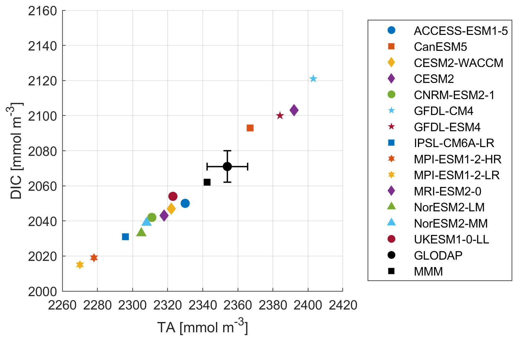
Figure 1 Global mean surface DIC [mmol m⁻³] versus TA [mmol m⁻³] of the 14 CMIP6 ESMs, the multi-model mean (MMM), and GLODAP including its error estimate.

3 Results

3.1 Analysis of CMIP6 alkalinity and DIC

The comparison of the models' simulated TA at the ocean surface to the GLODAP climatology shows that – on a global scale – most models underestimate surface TA and DIC, except for four models, CanESM5, GFDL-CM4, GFDL-ESM4, and MRI-ESM2-0, which simulate too much TA and DIC at the surface (Figs. 1, 2). The multi-model mean (MMM) is only slightly negatively biased (Figs. 1, 2). Global mean surface TA and DIC biases are strongly correlated (R=0.99, Fig. 1). Near-surface TA is strongly correlated with salinity, and upper-ocean salinity is governed by freshwater fluxes, e.g., precipitation and evaporation (Millero et al., 1998), and river flows (Cai et al., 2010). Overall, the comparison of salinity-normalized TA_n to GLODAP data shows bias patterns very similar to those of TA for all models. Most notably, some regional peculiarities that stem from salinity biases rather than biogeochemical processes are smoothed out (e.g., North Atlantic bias in NorESM; see Fig. S1 in the Supplement).

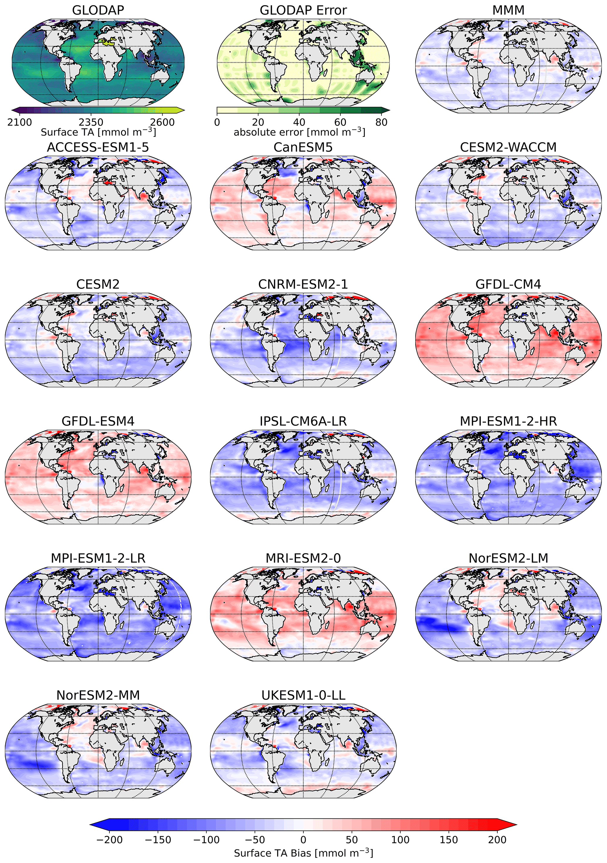
Figure 2 Surface distribution of TA in GLODAP (top left), its error estimate (top center), and the CMIP6 multi-model-mean (MMM) bias (top right), as well as the respective biases of the ESMs.

The vertical profiles of globally averaged TA and normalized TA_n (Fig. 3) show the aforementioned distribution of the CMIP6 models' surface biases as well, with most of the models showing less surface TA than GLODAP. The models mostly reproduce the features of the observed TA depth profile: the surface minimum, the subsurface maximum of TA, another minimum at around 500 m depth and the increase in TA with deeper depth (Fig. 3a). Two models of the same family (MPI-ESM1-2-LR and MPI-ESM1-2-HR) have less TA than the GLODAP product over the whole water column, and two models (GFDL-CM4 and GFDL-ESM4) have higher TA overall. This indicates that their global inventory of TA is too low (too high) compared to GLODAP. The explanation for the systematic low bias in the MPI model seems to be that too much TA was lost to the sediments during the model spin up (Koeve et al., 2014; Planchat et al., 2023). The high TA bias in the GFDL ESMs was apparently introduced in the post-processing step during the unit conversion from gravimetric (µmol kg⁻¹) to volumetric data (mmol m⁻³, common SI unit). The unit conversion is usually based on a chosen density value, which is not prescribed in modeling protocols. While most models chose a value between 1024 and 1028 kg m⁻³, the modeling group at GFDL apparently converted the units using a value of 1035 kg m⁻³ (Planchat et al., 2023). The profiles of the other models show either too little TA at the surface and too much at depth or vice versa, indicating that their TA inventory is closer to the observed one but that the TA distribution in the water column differs from the observations. Salinity normalization generally does not change the bias patterns (Fig. 3b). The salinity normalization does affect the shape of the profiles in the upper ocean. The surface minima and the subsurface maxima seen in TA disappear. Those features are essentially related to the upper-ocean salinity distribution.

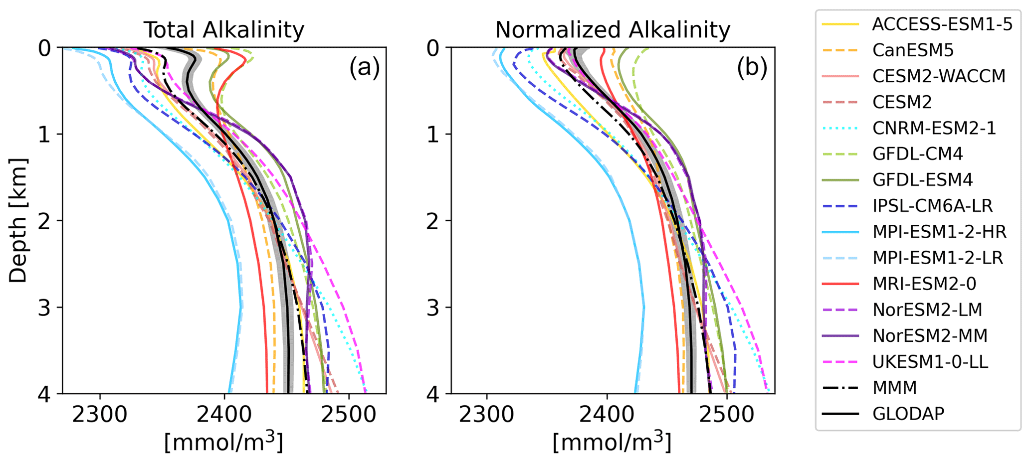
Figure 3 Vertical profiles of global mean TA (a) and TA_n (b) of the CMIP6 ESMs, the multi-model-mean (MMM), and GLODAP (black) with error estimate (grey shading).

The near-surface TA maximum seen in the global profile is also evident in the Atlantic, Pacific, and Indian oceans (Fig. 4). The high TA is related to the salinity maxima of subtropical underwater in the respective basins (Talley, 2002) and all models replicate this pattern. In the Atlantic Ocean, a TA minimum can be observed in the GLODAP data at around 800 m depth, which represents Antarctic Intermediate Water in the South Atlantic (low salinity) (Takahashi et al., 1981). This minimum is not well reproduced by the ESMs, referring to circulation biases. The relatively low TA in the deep Atlantic Ocean (compared to the Pacific and Indian oceans) between 1500 and 3500 m depth and the small gradient with depth are linked to North Atlantic Deep Water (NADW). Most models reproduce this pattern, while the CNRM, IPSL, and UK ESMs simulate a strong increase in TA below about 2000 m depth (Fig. 4b). Those three ESMs have a NEMO ocean model in common. The profile shapes in the Southern Ocean and Arctic Ocean are generally reproduced in terms of the TA gradients with depth, although the biases in absolute amount of TA present are visible here as well.

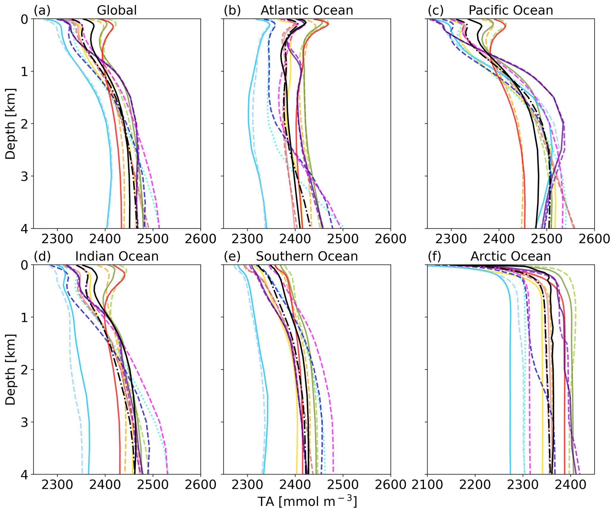
Figure 4 Global mean TA profiles for the major ocean basins. Color assignment is the same as in Fig. 3.

The surface DIC patterns compared to GLODAP show very similar patterns to those for TA in both general direction and local distribution (Fig. 5). The global mean surface biases in TA compared to GLODAP range from −85 mmol m⁻³ (−3.6 %) to +50 mmol m⁻³ (+2.1 %), where the MMM bias is −25 mmol m⁻³ (−1.1 %), and for the global mean surface DIC the biases range from −55 mmol m⁻³ (−2.6 %) to 53 mmol m⁻³ (+2.5 %), with the MMM bias being −13 mmol m⁻³ (−0.6 %). TA biases likely lead DIC biases, as DIC can adjust through gas exchange of CO₂ to maintain a surface chemical equilibrium with the atmospheric CO₂ concentration. Models with higher TA have higher DIC values and vice versa. We next investigate the origin of the models' alkalinity biases.

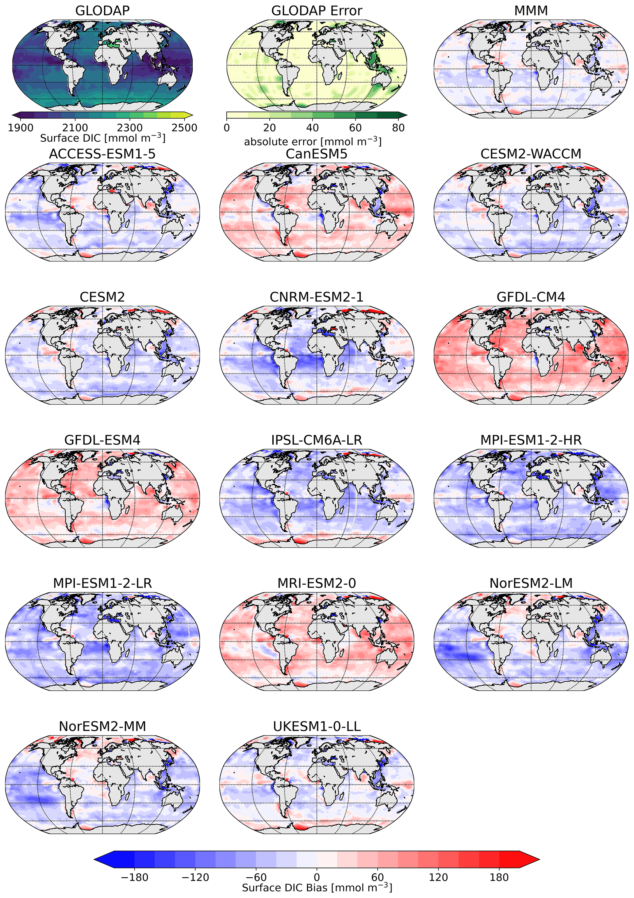
Figure 5 Surface distribution of DIC in GLODAP (top left), its error estimate (top center), and the CMIP6 multi-model mean (MMM) bias (top right), as well as the respective biases of the ESMs.

3.2 Decomposition of the vertical alkalinity biases

The goal of the TA^* method (Koeve et al., 2014) is to separate the TA bias into contributions from (1) an inadequate representation of ocean physics or forcings (e.g., circulation, freshwater flow, evaporation, and precipitation), (2) the parameterization of calcium carbonate (CaCO₃) formation and dissolution, and (3) the parameterization of organic matter remineralization processes. The first part, preformed alkalinity, includes the advection and upwelling of already biased water masses.

The decomposition of the TA biases (Fig. 6a) shows that in the upper 1 km most of the models' alkalinity biases are due to their preformed TA (Fig. 6b). Per definition, models with a negative surface TA bias have a negative bias in preformed TA. Below about 1000 m depth, TA⁰ stays constant with depth. TA biases from the representation of organic matter remineralization processes are on the order of 5 to 10 mmol m⁻³ and play only a negligible role in absolute terms (Fig. 6c). The bias in TA from calcium carbonate dissolution in the interior ocean (Fig. 6d) can in absolute terms be comparable to or even larger than the bias in preformed TA. The MRI model and the GFDL models have a small negative bias in TA^* on the order of ∼ 10–20 mmol m⁻³ that is relatively constant with depth. The MPI and NorESM models have a slight positive TA^* bias on about the same order of magnitude that is also relatively constant with depth, while the UKESM, the CNRM-ESM, and the IPSL-ESM exhibit TA^* biases that increase with depth. The CNRM model has the largest TA^* bias, with about 100 mmol m⁻³ at 4000 m depth. CNRM-ESM2-1 and IPSL-CM6A-LR both contain the same ocean model (NEMO) and the same biogeochemical model (PISCESv2). Dissolution in PISCESv2 is treated explicitly and is dependent on the calcite saturation state, and the sinking speed for particulate inorganic carbon (PIC) is depth-dependent, while for other models the sinking speed is constant. In two of the models (of Fig. 6d), MRI-ESM2-0 and UKESM1-0-LL, CaCO₃ is dissolved without a sediment, while the other models do have explicit sediment treatments where CaCO₃ is buried or dissolved, depending on either the calcite saturation state or a set rate (Planchat et al., 2023). A direct link of the treatment of CaCO₃ at the bottom to the bias at depths is not obvious in this case.

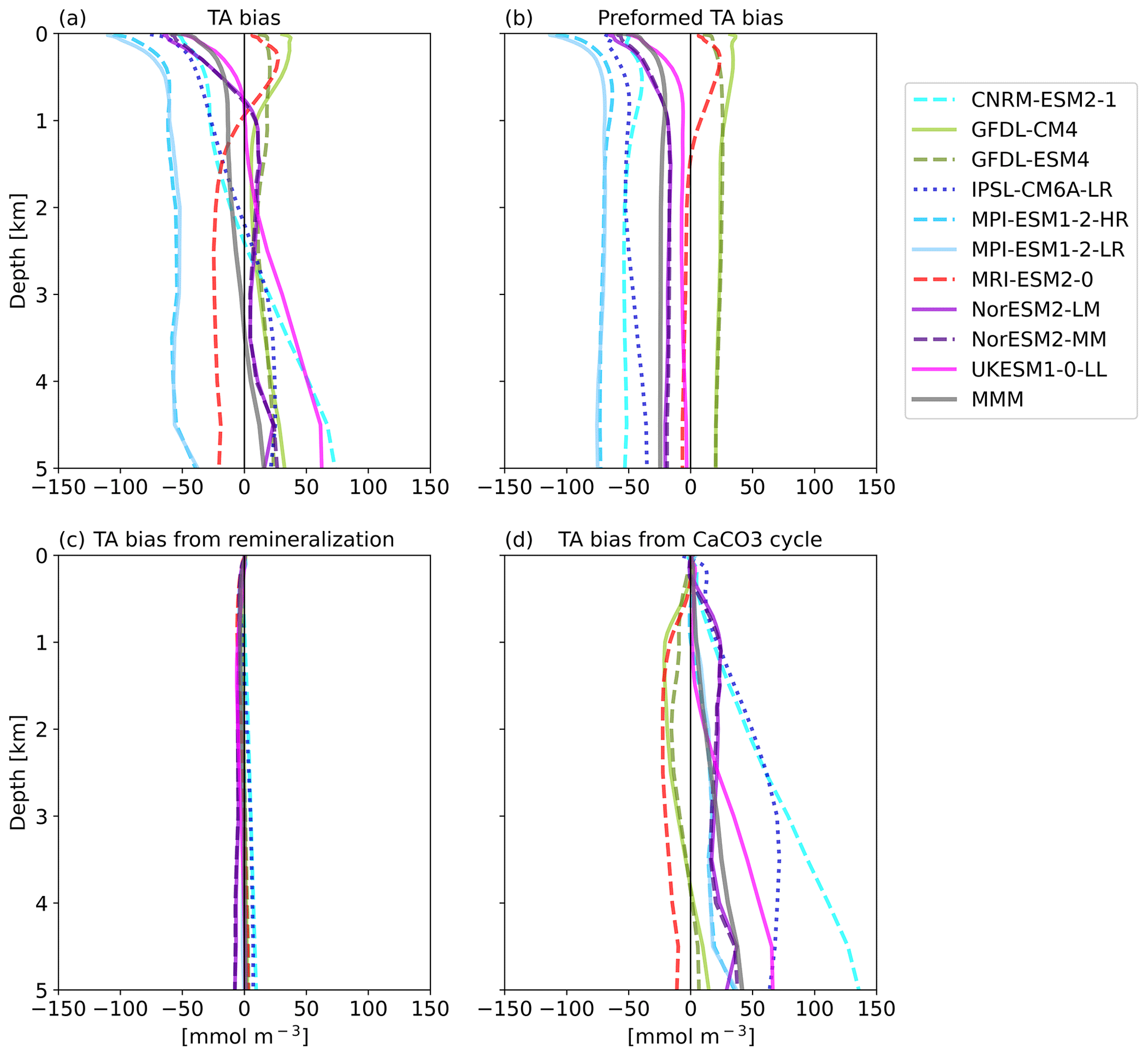
Figure 6 Globally averaged depth profiles of biases in (a) TA, (b) preformed TA (TA⁰), (c) TA from remineralization (TA^r), and (d) from calcium carbonate formation and dissolution (TA^*) in 10 CMIP6 models compared to the GLODAP climatology.

3.3 Impact of biases on OAE efficiency

Biases in simulated surface TA and DIC have implications for the individual models' efficiency of OAE. By causing biases in the Revelle factor, they also result in biases in initial surface ocean pCO₂ reduction after alkalinity addition, and final pCO₂ values after equilibration with the atmosphere might differ. In order to evaluate the range of this sensitivity, a back-of-the-envelope calculation was conducted using the ESMs' surface TA, DIC, pCO₂, and an alkalinity addition of 100 µmol kg⁻¹ to calculate the full carbonate system before and immediately after alkalinity enhancement and after assumed air–sea equilibration (see Sect. 2.3). The results from this calculation (Fig. 7b, d, e, f, g, h, i), together with the initial, unperturbed TA and TA–DIC ratios (Fig. 7a, c), are assessed for the ESMs and the MMM against the respective values for GLODAP.

The global mean Revelle factor from the CO2SYS computation for the GLODAP data set (10.19) is the third lowest in our compilation, and thus almost all ESMs have a higher Revelle factor than the GLODAP data, ranging from 10.18 to 10.54 (Fig. 7b). The Revelle factor is anti-correlated to the average TA–DIC ratio ($R=-\mathrm{0.99}$, Fig. 7c). In addition, the order of surface pH ($R=-\mathrm{0.96}$, Fig. 7g) and pCO₂ (R=0.97, Fig. 7d) values corresponds largely to each model's rank in Revelle factor (and thus also with the TA–DIC ratio). Models with a higher Revelle factor than GLODAP have a lower buffer capacity, which leads to already higher pCO₂ values (290 to 314 µatm) and lower pH (8.12 to 8.17) than in GLODAP (pCO₂: 292 µatm; pH: 8.16). Those models also show a greater initial reduction in surface ocean pCO₂ for the hypothetical addition of 100 µmol kg⁻¹ of TA ($R=-\mathrm{0.99}$, Fig. 7e) than GLODAP (−92 µatm), ranging from a 91 µatm to a 104 µatm decrease in pCO₂. Models with a higher Revelle factor also have a higher uptake efficiency, ηCO₂ (R=0.98, Fig. 7f). The initial change in pH after alkalinity addition (Fig. 7h) is about an order of magnitude larger than the change in pH after complete air–sea equilibration at constant atmospheric CO₂ (Fig. 7i). The respective changes in pH (non-equilibrated and equilibrated at constant atm CO₂) have a higher correlation to TA ($R=-\mathrm{0.92}$, $R=-\mathrm{0.99}$) than to the Revelle factor (R=0.83, R=0.63).

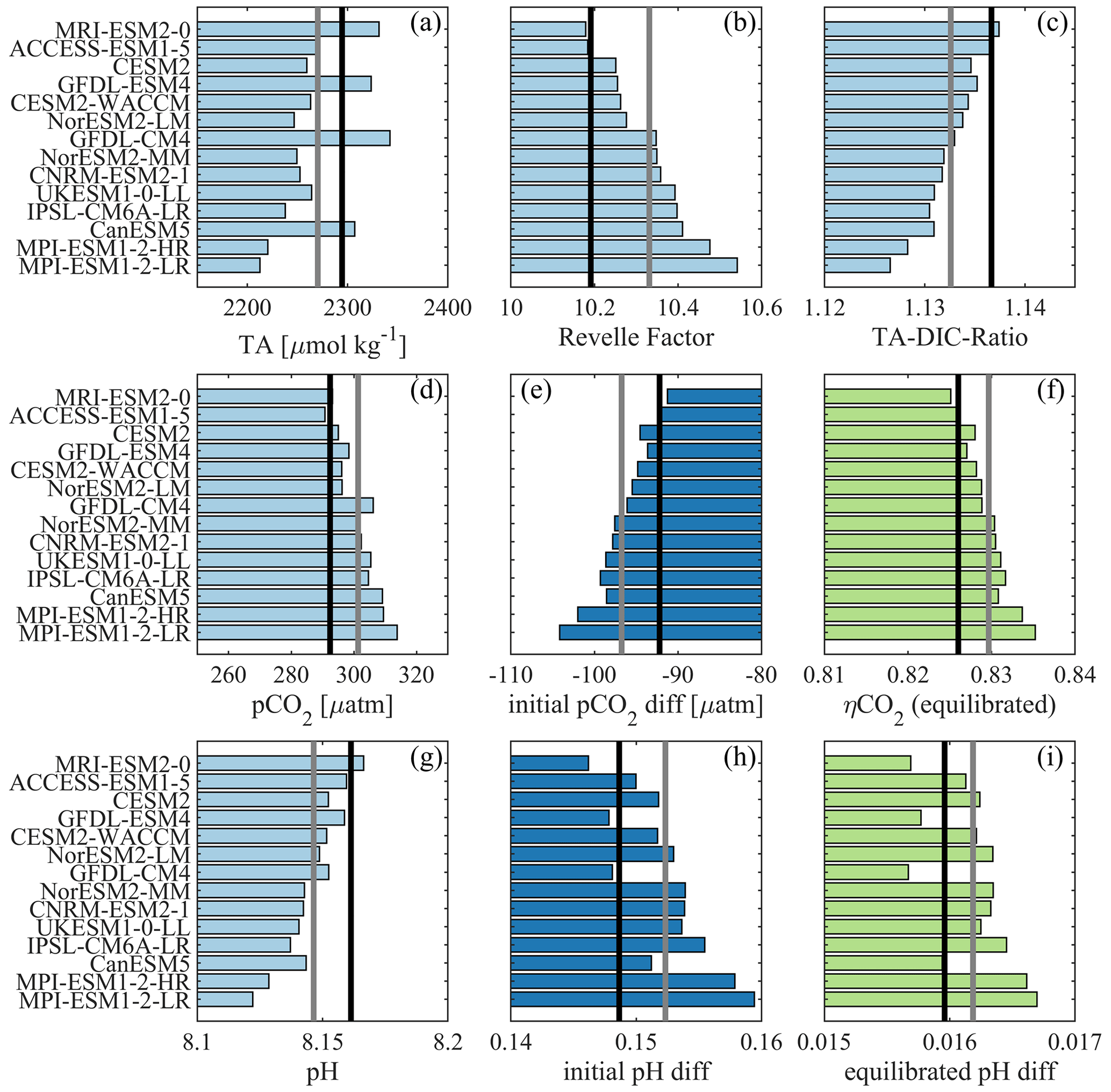
Figure 7 Carbonate system parameters were computed for all CMIP6 ESMs, the MMM (grey line), and the GLODAP data (black line) with the CO2SYS toolbox. The results are sorted by Revelle factor in ascending order for all panels. Shown are the TA (a), the Revelle factor (b), the TA–DIC ratio (c), initial pCO₂ (d), the difference in pCO₂ after a 100 µmol kg⁻¹ addition of TA (e), the uptake efficiency ηCO₂ (f), the initial pH (g), the difference in pH for constant DIC (h), and the difference in pH for constant pCO₂ (i). Light blue indicates the unperturbed mean state in the ESMs and GLODAP, dark blue indicates the initial state after OAE, and green indicates the state after OAE and subsequent air–sea equilibration.

In relative terms, we find that the ESMs' TA biases range from −3.6 % to +2.1 % with a mean of −1.1 % and that their DIC biases range from −2.6 % to +2.5 % with a mean value of −0.6 % (Fig. 1). Furthermore, the ESMs estimates of the initial pCO₂ decrease after a hypothetical TA enhancement by 100 µmol kg⁻¹ range from −1.0 % up to 13.0 % (mean 5.1 %) relative to GLODAP (Table S2). The controlling factor for this bias in initial pCO₂ reduction is in most cases the Revelle factor rather than the TA bias alone because the TA bias is always accompanied by a (partly) compensating DIC bias.

This simplified OAE example shows that for 12 out of 14 ESMs an increase of 100 µmol kg⁻¹ in TA would lead to a higher initial decrease in pCO₂ than observational data from GLODAP suggest. A higher sensitivity to TA changes due to a higher Revelle factor has also been shown in Hauck et al. (2016) during a decadal-scale OAE simulation. We additionally calculated the effect of the additions of 200, 500, and 1000 µmol kg⁻¹ of TA. The degree of pCO₂ overestimation decreases with the amount of TA added, but for a theoretical addition of 1000 µmol kg⁻¹ of TA the maximum initial pCO₂ reduction overestimate with respect to GLODAP is still 8 % (Table S2). We conclude that almost all ESMs might overestimate the initial pCO₂ difference in simulated OAE experiments. On the other hand, the CO₂ uptake efficiency computed with constant pCO₂ (equilibrated DIC) only differs by −0.1 % to 1.1 % (mean: 0.4 %) from the GLODAP value, and the ESMs may thus represent equilibrium CO₂ uptake rather robustly.

The initial increase in pH after alkalinity addition is relatively large (Fig. 7h, >0.1 pH units, i.e., on the same order of magnitude as the pH decrease since industrialization). However, after equilibration with the atmosphere (at presumed constant atmospheric CO₂), the lasting pH change is small (about 0.016, Fig. 7i). These pH changes are in line with previous quantifications (independent of the amount of alkalinity added; e.g., Köhler et al., 2013; Hartmann et al., 2013; Hauck et al., 2016), and their small magnitude is the direct result of the additional carbon uptake from the atmosphere. In emission-driven simulations, where atmospheric CO₂ is substantially reduced through large applications of alkalinization, pH increases more substantially (e.g., by <0.1 for an atmospheric CO₂ reduction of <100 ppm, Lenton et al., 2018; by >0.3 for an atmospheric CO₂ reduction of >1000 ppm in a multi-millennial simulation, Köhler, 2020). These findings call into question the commonly made statement that ocean alkalinization is unique as it “simultaneously mitigates atmospheric concentrations of CO₂ and ocean acidification” (Burt et al., 2021; Ilyina et al., 2013; National Academy of Science, 2021). While ocean alkalinity enhancement allows for additional CO₂ uptake at a pH level that does not drop any further, a restoration or rise in pH is only possible if (a) the water mass is not in contact with the atmosphere (perhaps for deep-ocean applications) or (b) ocean alkalinization is efficient in reducing atmospheric CO₂, which is the driver of ocean acidification. The latter case, however, applies to all land- and ocean-based CDR methods that are efficient in reducing atmospheric CO₂, and thus ocean alkalinity enhancement is not unique in this regard.

4 Discussion and conclusions

We evaluated CMIP6 models regarding their large-scale biases in TA and DIC compared to the gridded data set GLODAP. A total of 10 out of 14 ESMs underestimate surface TA (MMM: −25 mmol m⁻³; i.e., −1.1 %) and DIC (MMM: −13 mmol m⁻³; i.e., −0.6 %) with respect to observations. The range of the bias in TA is −85 mmol m⁻³ (−3.6 %) to 50 mmol m⁻³ (+2.1 %), and in DIC it is −55 mmol m⁻³ (−2.6 %) to 53 mmol m⁻³ (+2.5 %). This is a reversal from the TA and DIC representation in CMIP5, where most models and the MMM overestimated these variables, and the absolute and relative errors were at least twice as large as in CMIP6 (Planchat et al., 2023). The direction of the bias and the relative biases of TA and DIC have a direct impact on the Revelle factor and the initial pCO₂ reduction in the surface ocean after alkalinity addition (and thus affect CO₂ uptake) and should be known when assessing model experiments simulating OAE or other NETs that directly affect the ocean's carbonate chemistry. Terhaar et al. (2022) also found that CMIP6 models overestimate the Revelle factor and propose that CMIP6 models underestimate the anthropogenic ocean carbon sink from 1994 to 2007 by 9 %, of which around 3 % can be explained by the overestimation of the Revelle factor, while the remaining 6 % are related to the models' underestimation of the formation of mode and intermediate water in the Southern Ocean (Terhaar et al., 2021).

It is helpful to understand the contributions of the physical and biological pumps (soft tissue and calcium carbonate, respectively) to these TA biases in ESMs. The value of decomposing the carbon pump has already been recognized in previous studies (e.g., Sarmiento and Gruber, 2006; Kwon et al., 2009); however, there is not a common standard to achieve this decomposition. Here, we separated the global mean vertical TA bias into contributions from preformed alkalinity (TA⁰, physical pump), remineralization (TA^r, soft tissue pump), and alkalinity from calcification and carbonate dissolution (TA^*, CaCO₃ pump) following Koeve et al. (2014). This decomposition method aims to compute the physical contribution to the alkalinity distribution explicitly, similar to the method used in Oka (2020) and contrary to those of Sarmiento and Gruber (2006) and Planchat et al. (2023). An advantage of this method is that the preformed alkalinity is computed for each grid point and is therefore resolved spatially. In their presentation of the method, Koeve et al. (2014) note that the computation of TA^* according to Eqs. (2) to (4) reproduces tracer-based simulated TA^* robustly in most of the global ocean but that higher uncertainties occur in the Atlantic and in the 500 to a 1000 m layer in the Pacific and Indian oceans. Here, we only focused on the TA^* results for the global mean ocean. A caveat that was mentioned by Koeve et al. (2014) is that AOU is known to overestimate true oxygen utilization by 20 %–25 %. Hence, our TA^r computed from AOU probably also overestimates by this percentage. However, TA^r is rather small, and here we focus on the implication of the TA^* biases in ESMs and potential remedies for these biases.

The result from our TA^* analysis is that the global distribution of TA in ESMs is largely determined by preformed TA (especially in the upper ocean), which is set by ocean model physics (advection, overturning, mixing, etc.); however, this performed TA is not purely physical but also contains the physical redistribution of already biased TA. In the sub-surface and deep ocean, biases in TA are also driven by the CaCO₃ cycle, while contributions from remineralization are negligible. Although Planchat et al. (2023) do not assess alkalinity biases due to the physical carbon pump, they also point to a larger contribution of the carbonate pump relative to the soft tissue pump (remineralization) to the (normalized) TA biases. The model processes involving the physical distribution of TA are tuned to achieve the best overall model performance, and it could be tested whether a tuning to improve TA would support this goal. The findings regarding the contribution to the TA biases from the CaCO₃ cycle simulation suggest that improving the parameterizations of biogeochemical processes that are sources and sinks of TA, e.g., calcification, remineralization of sinking detritus, chemical dissolution of calcium carbonate, biological CaCO₃ formation, and dissolution, would be beneficial. Since the bias in TA from remineralization is small in all models, parameterizations that affect the calcium carbonate cycle are the most practical lever to improve the TA distribution for most models. This in turn needs a much-improved process understanding of CaCO₃ dissolution in microenvironments such as aggregates, zooplankton, and fish guts above the calcite and aragonite saturation horizons (Sulpis et al., 2021; Jansen and Wolf-Gladrow, 2001; Salter et al., 2017) from field and laboratory studies in order to mechanistically represent these processes and how they might be altered in a high-CO₂ ocean. In the absence of this mechanistic understanding, some suggestions to reduce TA biases are listed below.

Possibilities for model tuning include the following suggestions.

• If TA is low at the surface, decreasing the calcification (rate) within realistic limits or increasing near-surface dissolution could be beneficial (Gangstø et al., 2008; Gehlen et al., 2007).

• If the calcite dissolution is prescribed to increase with depth (Yamanaka and Tajika, 1996), this process could be tuned to better match the observed vertical distributions of calcite or TA.

Possible improvements in model parameterizations include the following suggestions.

• If calcite dissolution is formulated as (mostly) saturation dependent and is therefore (close to) zero above the calcite saturation horizon, a term should be implemented that encompasses dissolution processes that have been observed to occur above said horizon, e.g., calcite dissolution in microenvironments like marine snow and zooplankton guts (Sulpis et al., 2021). It was shown that the acidic environment in guts of starving copepods can dissolve up to 38 % of the calcite taken up by grazing (White et al., 2018). For non-starving copepods this value was somewhat lower (Pond et al., 1995; Jansen and Wolf-Gladrow, 2001).

• In addition to those processes, it is known that aragonite and high-magnesium calcite have a shallower saturation horizon than calcite and contribute to upper-ocean calcium carbonate dissolution (Sabine et al., 2002; Gangstø et al., 2008; Barrett et al., 2014; Battaglia et al., 2016). Almost all models only simulate calcite explicitly (Planchat et al., 2023), which is a deficit since Buitenhuis et al. (2019) proposed that aragonite-producing pteropods might contribute at least 33 % to export of CaCO₃ at 100 m and up to 89 % to the pelagic calcification. Although exact numbers might be subject to reevaluation when more data become available, a carbon cycle formulation expanded to also simulate aragonite (formation and dissolution) may be beneficial for a more realistic alkalinity distribution.

• The representation of CaCO₃ treatment at the bottom sediment interface (dissolution, sedimentation, sediment weathering) is important for the total alkalinity budget and also for upper-ocean alkalinity, especially in more shallow regions where alkalinity-enriched waters (through dissolution) can recirculate to the upper ocean more quickly (Gehlen et al., 2007).

The back-of-the-envelope calculations of the ESMs' carbonate system states revealed that all but two of the models have a higher global mean Revelle factor than calculated from GLODAP, correlated with a higher TA–DIC ratio than suggested by observations (see also Terhaar et al., 2022). For a hypothetical addition of 100 µmol kg⁻¹ TA this bias leads to an overestimation of the initial pCO₂ reduction by up to 13 % (affecting CO₂ uptake from the atmosphere). The addition of just 100 µmol kg⁻¹ TA is actually at the very low end of the spectrum used in past and current OAE experiments in models and in mesocosms (Hartmann et al., 2023; Ferderer et al., 2022). This calculation is a simplified exercise since gas exchange between ocean and atmosphere is not accounted for and neither are the potential precipitation or sinking of calcium carbonate (Hartmann et al., 2023). The CO₂ uptake efficiency factor, ηCO₂, relates changes in surface DIC to alkalinity input. We computed this metric here with constant pCO₂ after alkalinity addition, which suggests complete equilibration and neglects any reduction in atmospheric CO₂ due to OAE. Studies suggest that the timescale and efficiency of the equilibration can differ immensely depending on the ocean region. He and Tyka (2023) found that after 1 year ηCO₂ varied between 0.2 and 0.85 and that after 10 years most locations showed an uptake fraction of 0.65–0.80. Jones et al. (2014) quantified the mean global air–sea equilibration timescale for CO₂ at 4.4 months (range of 0.5 to 24 months regionally). Bach et al. (2023) suggest a pragmatic timescale of 10 years for a 95 % DIC equilibration after OAE measures. It is within this range of suggested equilibration timescales that the differences in simulated pCO₂ change between ESMs are important.

The results of our idealized calculation also highlight the need to monitor at least two carbonate system variables to characterize the full carbonate system after alkalinity addition in a potential real-world application. Knowing the amount of alkalinity added and then monitoring pCO₂ with an autonomous sensor will not be sufficient to characterize the full carbonate system and the level of equilibrium reached, particularly as alkalinity and carbon will be subject to transport through mixing and advection. Autonomous sensors with high accuracy are currently only available for pCO₂, whereas alkalinity sensors are not commercially available (see review in Ho et al., 2023) and pH sensors do not have high enough accuracy (Wimart-Rousseau et al., 2023). This poses a challenge for monitoring, reporting, and verification (MRV) that may be tackled through (i) measuring discrete water samples until technical advances make autonomous measurements of two carbonate system variables possible or (ii) using models of high fidelity. In order to fully capture the effect of OAE on atmospheric CO₂ concentration and the model spread related to biases stemming from circulation and biogeochemical assumptions, model OAE experiments need to be performed in a suite of fully coupled emission-driven ESMs with a precise protocol and with realistic representation of the carbonate pump, including CaCO₃ dissolution above the carbonate saturation horizon, which is not even sufficiently understood in the real world (Sulpis et al., 2021).