A modeling approach to investigate drivers, variability and uncertainties in O₂ fluxes and O₂ : CO₂ exchange ratios in a temperate forest

The O₂ : CO₂ exchange ratio (ER) between terrestrial ecosystems and the atmosphere is a key parameter for partitioning global ocean and land carbon fluxes. The long-term terrestrial ER is considered to be close to 1.10 mol of O₂ consumed per mole of CO₂ produced. Due to the technical challenge in measuring directly the ER of entire terrestrial ecosystems (ER_eco), little is known about variations in ER at hourly and seasonal scales, as well as how different components contribute to ER_eco. In this modeling study, we explored the variability in and drivers of ER_eco and evaluated the hypothetical uncertainty in determining ecosystem O₂ fluxes based on current instrument precision. We adapted the one-dimensional, multilayer atmosphere–biosphere gas exchange model “CANVEG” to simulate hourly ER_eco from modeled O₂ and CO₂ fluxes in a temperate beech forest in Germany.

We found that the modeled annual mean ER_eco ranged from 1.06 to 1.12 mol mol⁻¹ within the 5-year study period. Hourly ER_eco showed strong variations over diel and seasonal cycles and within the vertical canopy profile. The determination of ER from O₂ and CO₂ mole fractions in air above and within the canopy (ER_conc) varied between 1.115 and 1.15 mol mol⁻¹. CANVEG simulations also indicated that ecosystem O₂ fluxes could be derived with the flux-gradient method using measured vertical gradients in scalar properties, as well as fluxes of CO₂, sensible heat and latent energy derived from eddy covariance measurements. Owing to measurement uncertainties, however, the uncertainty in estimated O₂ fluxes derived with the flux-gradient approach could be as high as 15 µmol m⁻² s⁻¹, which represented the 90 % quantile of the uncertainty in hourly data with a high-accuracy instrument. We also demonstrated that O₂ fluxes can be used to partition net CO₂ exchange fluxes into their component fluxes of photosynthesis and respiration if ER_eco is known. The uncertainty of the partitioned gross assimilation ranged from 1.43 to 4.88 µmol m⁻² s⁻¹ assuming a measurement uncertainty of 0.1 or 2.5 µmol m⁻² s⁻¹ for net ecosystem CO₂ exchange and from 0.1 to 15 µmol m⁻² s⁻¹ for net ecosystem O₂ exchange, respectively. Our analysis suggests that O₂ measurements at ecosystem scale have the potential to partition net CO₂ fluxes into their component fluxes, but further improvement in instrument precision is needed.

1 Introduction

Fluxes of O₂ and CO₂ between the terrestrial biosphere and atmosphere are inversely linked in photosynthesis, which assimilates CO₂ and releases O₂, and in respiration, which consumes O₂ and releases CO₂ (Keeling and Manning, 2014; Keeling and Shertz, 1992a; Krogh, 1919; Severinghaus, 1995). The relationship between these opposing fluxes can be described with the so-called O₂ : CO₂ exchange ratio (ER; see Table S1 in the Supplement for an overview of all abbreviations and variable names used here), which should be considered on various temporal and spatial scales – ranging from hourly to decadal scales temporally and from leaf to global scales spatially. Since the relationship of O₂ and CO₂ fluxes between the atmosphere and different carbon reservoirs (terrestrial biosphere, oceans and fossil fuels) differs on regional and global scales, these different ERs can be applied as parameters in global models in conjunction with observations of atmospheric O₂ and CO₂ abundances to quantify the global sinks of CO₂ into the ocean and the terrestrial biosphere (Battle et al., 2000; Ishidoya et al., 2012; Keeling and Manning, 2014; Keeling and Shertz, 1992b; Tohjima et al., 2019). The global ER for the terrestrial biosphere is commonly set to 1.10 mol of O₂ consumed per mole of CO₂ produced (or vice versa) (Severinghaus, 1995) by assuming that this value, derived from elemental abundance data, is a representative long-term average for all land biota (Keeling and Manning, 2014; Manning and Keeling, 2006). An ER of 1.05 mol mol⁻¹ was determined by Randerson et al. (2006) based on observed chemical compositions of plant parts for the quantification of the global carbon sink. Measurements using the oxidative ratio of organic material provided a more recent terrestrial ER estimate of 1.04 ± 0.03 mol mol⁻¹ (Worrall et al., 2013). Using an ER of 1.05 mol mol⁻¹ instead of 1.10 mol mol⁻¹ in carbon budget models will contribute 0.05 Pg C yr⁻¹ more to the global land carbon sink and an equivalent amount less to the ocean carbon sink (Keeling and Manning, 2014), indicating that the ER needs to be well constrained when parameterized in global ocean and land carbon cycle models.

On an ecosystem scale, a mole-fraction-based and a flux-based O₂ : CO₂ ratio can be considered (Ishidoya et al., 2013; Seibt et al., 2004). The former is defined as the fluctuations in the mole fraction of O₂ per mole fraction of CO₂ in the atmosphere (ER_conc). Thus, ER_conc is usually derived from the slopes of linear regressions between observed atmospheric O₂ and CO₂ mole fractions (Battle et al., 2019; Ishidoya et al., 2013; Seibt et al., 2004). Battle et al. (2019) observed an average ER_conc=1.08 ± 0.007 mol mol⁻¹ in a mixed deciduous forest over a 6-year period with temporal variations on a 6 h basis ranging between 0.85 and 1.15 mol mol⁻¹. Measurements of canopy air O₂ and CO₂ mole fractions at two different forest sites yielded ER_conc estimations between 1.01 and 1.03 mol mol⁻¹ averaged over 24 h periods and between 1.14 and 1.19 mol mol⁻¹ during daytime only (Seibt et al., 2004). Ishidoya et al. (2013) obtained differing ER_conc at two heights within a cool temperate deciduous forest, reflecting variations in ER_conc with canopy height. Furthermore, they observed different ER_conc during daytime (0.87 mol mol⁻¹) and nighttime (1.03 mol mol⁻¹) in summer, indicating a significant variation in ER_conc over the diel period (Ishidoya et al., 2013). Faassen et al. (2023) found much higher ER_conc over 24 h (2.05 ± 0.03 mol mol⁻¹) than for daytime only (1.10 ± 0.12 mol mol⁻¹) and nighttime only (1.22 ± 0.02 mol mol⁻¹) due to variations in the boundary layer height during the measurement period.

The flux-based O₂ : CO₂ ratio is defined as the O₂ flux per CO₂ flux between an ecosystem and the atmosphere (ER_eco). Flux estimates can be described as the net turbulent exchange or the overall net exchange (turbulent plus storage flux), and we focused on the latter in this study. Very few studies have attempted to quantify ER_eco because measuring O₂ fluxes at ecosystem scale is still a major challenge. Since O₂ and CO₂ are strongly anti-correlated in the processes of photosynthesis and respiration, changes in both scalars are very similar in absolute numbers, typically on the order of a few parts per million. However, the relative changes in O₂ are much smaller than in CO₂ owing to the much higher atmospheric abundance (around 210 000 ppm for O₂ and around 400 ppm for CO₂), making O₂ measurements at sufficient precision and accuracy technically challenging. Thus, previous studies resorted to, for instance, the flux-gradient method, chamber measurements and modeling approaches. Ishidoya et al. (2015) determined a daily mean net turbulent ER = 0.86 mol mol⁻¹ based on O₂ and CO₂ gradient measurements. Faassen et al. (2023) reported daytime and nighttime ER_eco as 0.92 ± 0.17 and 1.03 ± 0.05 mol mol⁻¹, respectively. In general, ER_eco depends on the elemental composition and reduction state of organic material and on the temporal variation and spatial distribution of sinks and sources of ecosystem flux components (Seibt et al., 2004). As described by Battle et al. (2019), the dynamics and interrelations of the various sinks and sources within the ecosystem, each with their own ER_eco, result in the mixed signal ER_conc.

Current micrometeorological approaches to measure gas exchange between ecosystems and the atmosphere include eddy covariance, flux-gradient and eddy accumulation methods, which could all theoretically be used to determine ecosystem O₂ fluxes. The applicability of the eddy covariance technique for O₂ flux estimation, however, requires high precision at a high measurement frequency (10–20 Hz). Except for a homemade, non-commercial vacuum ultraviolet (VUV) absorption analyzer (Stephens et al., 2003), no suitable instrument exists so far. The application of the eddy accumulation method is also technically challenging and has not yet been applied to O₂ (Emad and Siebicke, 2023a, b).

With the flux-gradient method, O₂ fluxes can be inferred from an O₂ gradient above a canopy and from an eddy diffusivity (K), which can be derived based on additional CO₂, sensible heat or latent heat flux measurements (Baldocchi et al., 1988). This method assumes that heat and mass are transported in a similar manner between two adjacent levels above the canopy (Baldocchi et al., 1988). The method's applicability is again particularly challenging for O₂ estimates owing to the typically large measurement uncertainty in relation to the small O₂ gradient. One approach to increase the measurement-to-noise ratio is to move the lower inlet of the gradient measurement closer to or even inside the canopy. This approach, however, violates the assumption of the flux-gradient method owing to infrequent but predominantly large eddies within the canopy, counter-gradient fluxes and possible non-differentiable gradients (Raupach, 1989; Wilson, 1989). The flux-gradient method has already been used for O₂ flux estimation above a cool temperate forest (Ishidoya et al., 2015), an urban canopy (Ishidoya et al., 2020) and a boreal forest (Faassen et al., 2023). The theoretical limits of the flux-gradient method for O₂ fluxes given current instrument precision and accuracy, however, have not yet been fully explored.

Chamber-level gas exchange measurements provide an alternative approach to measure the ER of individual components such as leaf, stem and soil, which could be scaled up to ecosystem level. Branch and soil chamber measurements in a German temperate forest showed an average ER of leaf net assimilation (ER_An; net assimilation defined as carboxylation minus photorespiration and dark respiration) between 1.08 ± 0.16 and 1.19 ± 0.12 mol mol⁻¹, as well as an ER of soil respiration (ER_soil) of 0.94 ± 0.04 mol mol⁻¹ (Seibt et al., 2004). In a cool temperate deciduous forest in Japan, chamber measurements indicated an ER_An=1.02 ± 0.03 and ER_soil=1.11 ± 0.01 mol mol⁻¹ (Ishidoya et al., 2013). Hilman et al. (2019) measured an average ER of stem respiration (ER_stem) between 0.97 and 1.95 mol mol⁻¹ for tropical, temperate and Mediterranean trees with a closed-flow chamber system with two continuous flow analyzers.

The ER variability in assimilation and respiration fluxes found in these studies provides a potential approach to partition net CO₂ fluxes into their components following similar approaches based on stable isotopes in CO₂ (Knohl and Buchmann, 2005; Ogee et al., 2004; Wehr and Saleska, 2015; Zobitz et al., 2007). Using simultaneous measurements of net ecosystem O₂ and CO₂ fluxes and considering the ER for the photosynthetic and respiratory processes in a canopy and at the soil surface, two mass balance equations can be written for O₂ and CO₂ (see Eq. 1 below). Hourly or half-hourly ER would need to agree with the typical time step of flux estimates derived with the eddy covariance technique, which is the standard method of measuring gas exchange between land surfaces and the atmosphere (Baldocchi et al., 2001; Goulden et al., 1996). Theoretically, such an O₂-based partitioning method only works for periods when the ER of gross assimilation (ER_A) and ER of gross ecosystem respiration (ER_R) differ because a second independent mass balance equation is needed to yield CO₂ fluxes of assimilation (F_A) and respiration (F_R). According to Ogee et al. (2004), the difference in ER has to be large enough to obtain a reasonable accuracy in the partitioned net CO₂ fluxes. Consequently, an analysis of temporal dynamics in ER_A and ER_R is necessary in order to evaluate the possibility of applying O₂ observations in a CO₂ flux-partitioning approach.

The contribution of flux components to the temporal and spatial variability in overall ecosystem O₂ fluxes can also be explored by modeling approaches. For example, net turbulent ER was simulated with a simple one-box model with daily time steps by assuming that O₂ and CO₂ mole fractions are spatially constant and temporally variable within the canopy (Ishidoya et al., 2015; Seibt et al., 2004). These simulations indicated that variations in net turbulent ER are influenced not only by leaf and soil fluxes but also by turbulence inside and outside the canopy (Seibt et al., 2004). To explore the drivers of ER variations at the ecosystem scale, more precise turbulence effects need to be considered. However, simple one-box models assume uniform and well-mixed air columns throughout the canopy, with the result that modeled ER lacks variations for different layers within the canopy.

Multilayer atmosphere–biosphere models such as CANVEG (Baldocchi, 1997; Baldocchi and Wilson, 2001) differ from one-box models in that they are designed to represent the temporal and (vertical) spatial scale of an eddy covariance tower. Therefore, they are a good simulator to test and examine new types of observations (Oikawa et al., 2017). CANVEG includes within-canopy transport of CO₂, water vapor and energy (Baldocchi, 1997; Baldocchi and Wilson, 2001), with the result that if it were adapted to O₂ processes, one could evaluate the accuracy of different flux measurement techniques such as eddy covariance or flux-gradient approaches. Published ER values of gross and/or net assimilation, stem respiration, and soil respiration can be employed as parameters to derive component-specific O₂ fluxes from existing modeled CO₂ fluxes. Thus, concurrent O₂ and CO₂ fluxes and ER can be plausibly simulated for multiple canopy layers and for the whole ecosystem, with which we can analyze the main drivers of modeled ER values, their diel and seasonal variability, and vertical variations. In addition, concurrently simulated mole fraction profiles – a function of turbulent dispersion and the strength and location of scalar sources and sinks – enable us to test the precision of the flux-gradient method for O₂ flux estimation while choosing various measurement heights inside and above the canopy. Furthermore, the performance of an O₂-based source-partitioning method can be evaluated based on model simulations.

Given these considerations, we defined the following objectives for this study: (1) to implement atmosphere–biosphere O₂ : CO₂ exchange ratios for various ecosystem components in the multilayer CANVEG model; (2) to explore temporal and spatial variations in O₂ : CO₂ exchange ratios at ecosystem scale, as well as the underlying main drivers at ecosystem scale; (3) to evaluate the potential precision of the flux-gradient approach to obtain O₂ fluxes; and (4) to evaluate the feasibility of O₂ flux measurements for CO₂ flux partitioning.

2 Methods

2.1 Site description

The meteorological and plant-specific ecophysiological measurements used in our model simulation were derived from the Leinefelde FLUXNET tower site (DE-Lnf; https://doi.org/10.18140/FLX/1440150) located in central Germany (51^∘19^′42^′′ N, 10^∘22^′04^′′ E; 450 m a.s.l.; Anthoni et al., 2004). The vegetation at the site is an even-aged managed beech stand (Fagus sylvatica L.) with an age of approximately 130 years (Tamrakar et al., 2018). Between 2002 and 2016, the mean annual temperature was 8.3 ± 0.7 ^∘C and the average cumulative annual precipitation was 600 ± 150 mm (Braden-Behrens et al., 2019). The canopy height (ht) was 37.5 m, and the effective leaf area index (LAI) was at maximum 4.8 m² m⁻² in the growing season in 2015 (Braden-Behrens et al., 2017).

Meteorological variables are continuously measured including air temperature, air humidity, direct and diffuse global radiation, photosynthetic photon flux density, wind velocity, air pressure, vapor pressure deficit, precipitation, atmospheric CO₂ mole fraction (CO_2 atm), soil temperature, and soil moisture. Also, fluxes of net ecosystem CO₂ exchange ($F_{{\mathrm{CO}}_{\mathrm{2}}}$), sensible heat (H) and latent heat (LE) are obtained with the eddy covariance technique at 44 m above the ground level (Anthoni et al., 2004). The meteorological variables were used as input data for our model simulations, while the flux estimates were storage-term-corrected and then used for model calibration and validation (see below). In this paper, upward fluxes (release to the atmosphere) are presented as positive quantities and downward fluxes (uptake by the ecosystem) as negative quantities. Thus, O₂ fluxes always have opposite signs to their corresponding CO₂ fluxes, which is in line with micrometeorological conventions.

2.2 Model description and model setup

We used the one-dimensional, multilayer atmosphere–biosphere gas exchange model “CANVEG”, described by Baldocchi (1997) and Baldocchi and Wilson (2001). The model domain included 120 model layers above the ground, in which the lower 40 aboveground layers covered the entire canopy, while the bottom layer represented the soil surface for the description of soil carbon and energy fluxes. The domain also included 10 belowground soil layers; however, this study did not consider processes within the soil column in any detail. CANVEG used hourly meteorological variables as drivers, as well as site-specific parameters (see Table 1), to simulate atmosphere–biosphere water vapor, CO₂ and energy fluxes within and above the forest canopy.

Table 1 Model parameters adjusted to the study site Leinefelde, Germany.

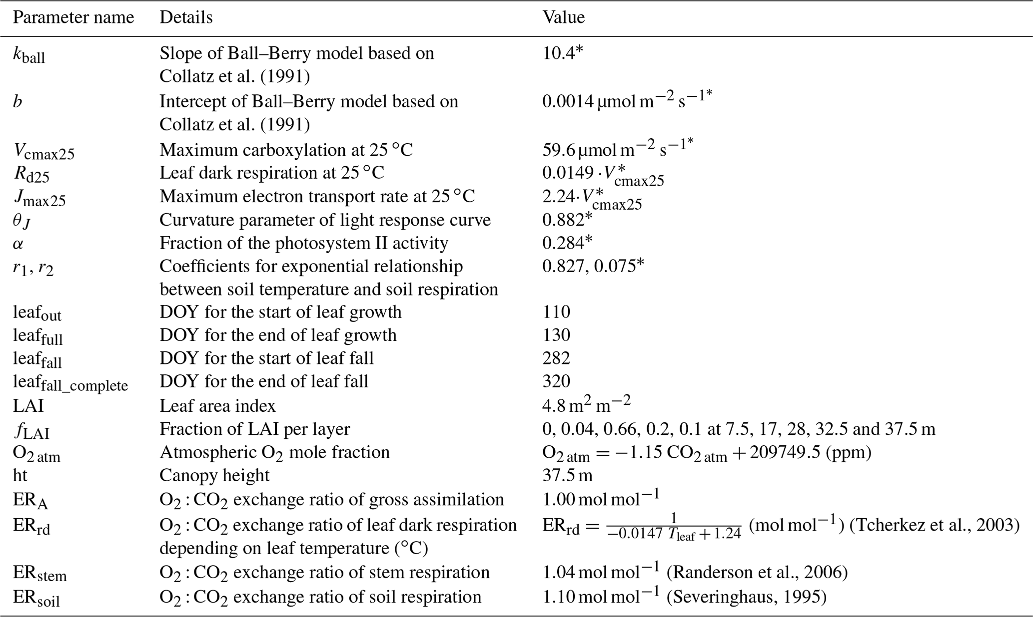
^∗ Parameters were calibrated with eddy covariance measurements of hourly $F_{{\mathrm{CO}}_{\mathrm{2}}}$, F_R, H and LE in 2012 and 2013 via the Markov chain Monte Carlo (MCMC) method.

The carbon, water and energy modules in CANVEG have been validated for various environmental conditions and forest types (Baldocchi, 1997; Baldocchi et al., 2002, 1999). Moreover, CANVEG has previously been applied to an unmanaged beech-dominated forest site only 30 km away from the site of this study (Knohl and Baldocchi, 2008) and has recently been used to simulate the isotopic composition of carbon assimilates at Leinefelde (Braden-Behrens et al., 2019). We translated the original C code (Baldocchi, 1997) to Fortran 90, which was then used for further implementations.

Atmospheric O₂ mole fraction (O_2 atm) as an input for the model was deduced from a fixed O₂ : CO₂ mole ratio of −1.15 mol mol⁻¹ and continuous CO₂ mole fraction measurements at the site (Table 1). The fixed O₂ : CO₂ mole ratio was derived from measurements at the University of Göttingen from November 2017 to January 2018 using a high-precision O₂ measurement system developed by Penelope Pickers (University of East Anglia, UK), which is very similar to the system described in Pickers et al. (2017). For these measurements, the correlation between O₂ and CO₂ mole fractions had R²=0.99.

Some model parameters regarding leaf photosynthesis, stomatal conductance and soil respiration were fitted to the actual site conditions via the Markov chain Monte Carlo (MCMC) method (Van Oijen et al., 2005). Eddy covariance measurements of hourly $F_{{\mathrm{CO}}_{\mathrm{2}}}$, H and LE, as well as the estimated ecosystem respiration (F_R) in 2012 and 2013, were used to calibrate the model parameters (Table 1). The years 2014–2016 were used for model validation. The leaf phenology parameters, including day of year (DOY) for the start of leaf growth, end of leaf growth, start of leaf fall and end of leaf fall (leaf_out, leaf_full, leaf_fall and leaf_{fall_complete}), were derived from daily camera images in 2015 above the canopy. LAI during the course of a year was simulated based on these four parameters: the DOY range before leaf_out and after leaf_{fall_complete} was defined as winter when LAI = zero, and the DOY range between leaf_full and leaf_fall was defined as summer when LAI = 4.8 m² m⁻². During spring (leaf_out < DOY  < leaf_full) and during autumn (leaf_fall < DOY < leaf_{fall_complete}) LAI increased or decreased linearly, respectively. The maximum LAI of 4.8 m² m⁻² and the LAI fraction (f_LAI) at five different heights in the canopy were measured using a LI-2000 plant canopy analyzer (LI-COR Biosciences GmbH, Germany) in 2015 (Braden-Behrens et al., 2017). The vertical LAI profile was assumed to follow a beta distribution, which was fitted to the observed f_LAI (Table 1). This relationship between LAI and height (z) allocates leaves mainly in the upper canopy ($z/\mathrm{ht}$ ≥ 0.45) with almost no leaves in the bottom canopy (Fig. 1a). The wood area index (WAI) consisted of the branches (80 % of total WAI) and the stems (20 % of total WAI). The branches were situated in the upper canopy ($z/\mathrm{ht}$ ≥ 0.45) following the same distribution algorithm as LAI, while in the lower canopy ($z/\mathrm{ht}$ < 0.45), the fraction of stem WAI per layer to total stem area was deduced from the fraction of stem diameter per layer to the diameter at breast height (f_DBH) as a function of height (z): f_DBH = 102 − 2.6z + 0.08z² − 0.0023z³ (Grundner et al., 1952). This setup of the forest canopy including leaf phenology and the vertical LAI and WAI profiles was used for all years of the model run. All site-specific parameters used in this study are listed in Table 1.

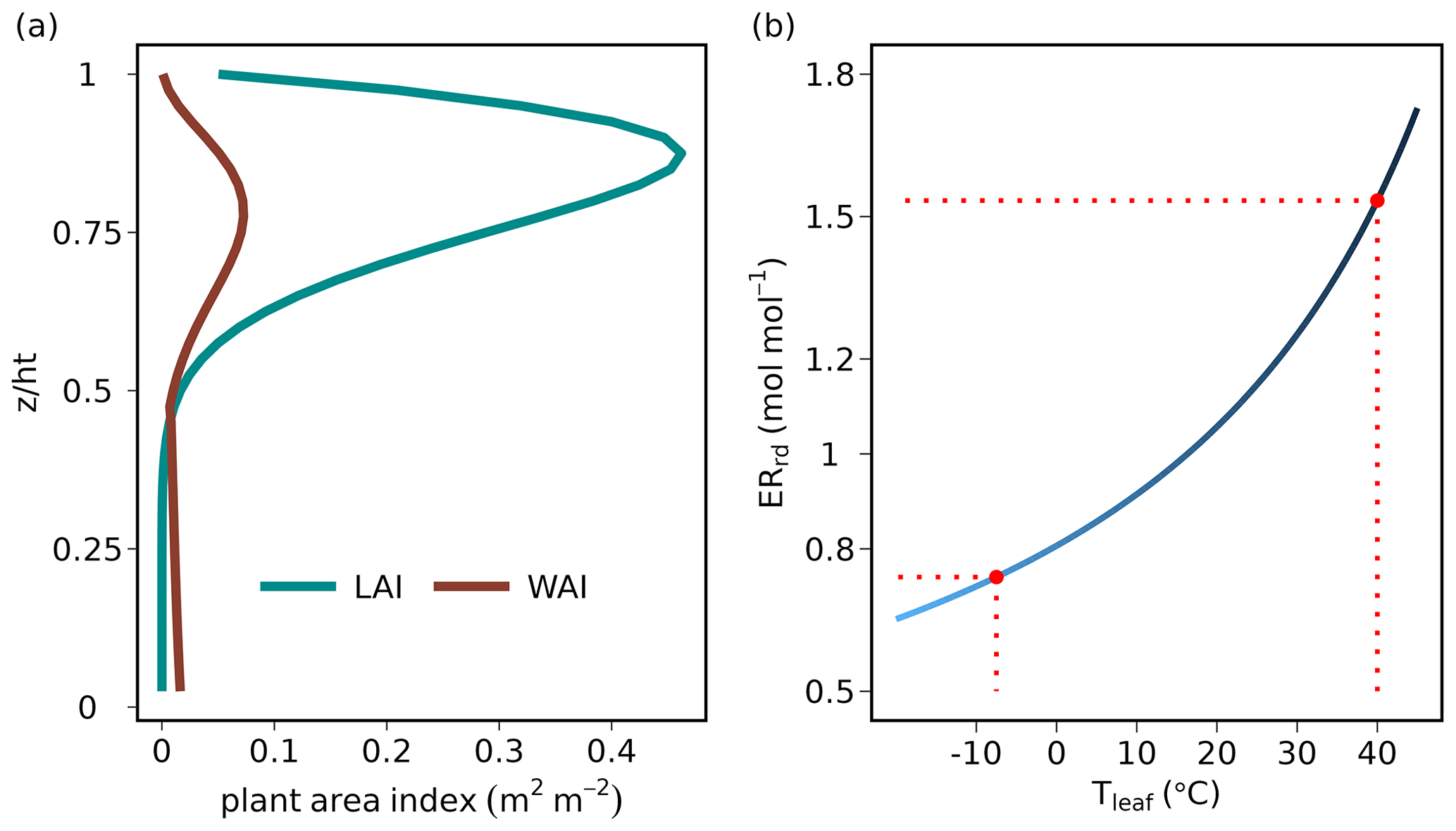
Figure 1 (a) Distribution of vertical leaf and wood area indices (LAI and WAI in m² m⁻² per canopy layer) used in the CANVEG model, derived from measurements at the Leinefelde study site (Braden-Behrens et al., 2017). The y axis is the ratio of the height in the canopy (z) to the top of the canopy (ht). (b) O₂ : CO₂ exchange ratio of leaf dark respiration (ER_rd in mol mol⁻¹) as a function of leaf temperature (T_leaf in ^∘C) after Tcherkez et al. (2003). The dashed red lines indicate the range of T_leaf and corresponding ER_rd in this study.

For the simulation of net ecosystem O₂ fluxes ($F_{{\mathrm{O}}_{\mathrm{2}}}$), values of ER had to be chosen: the input parameter of ER_A was set to 1.00 mol mol⁻¹ (Table 1) by assuming that photosynthesis produces glucose (C₆H₁₂O₆), resulting in equal O₂ and CO₂ fluxes. The ER of canopy respiration was attributed to the ER of leaf dark respiration (ER_rd) and stem respiration (ER_stem). ER_stem was fixed to 1.04 mol mol⁻¹ (Randerson et al., 2006), while the ER_rd was set to increase with leaf temperature (T_leaf; Fig. 1b) according to Tcherkez et al. (2003). ER_soil was set to 1.10 mol mol⁻¹ (Randerson et al., 2006; Severinghaus, 1995). To quantify the dependency of the CANVEG model regarding these fixed ER parameters, we also conducted a sensitivity analysis, where we changed ER_A, ER_stem and ER_soil each by ± 10 % and estimated the resulting relative changes in simulated O₂ fluxes. Furthermore, the impact of changed ER parameters was also investigated in the following parts of this study (see Sect. 2.3 and 2.5 below).

To validate the model, we used eddy covariance measurements of $F_{{\mathrm{CO}}_{\mathrm{2}}}$, H and LE from 2014 to 2016. To quantify the model performance, we calculated the slope, intercept and the coefficient of determination (R²) of a linear regression between modeled and observed $F_{{\mathrm{CO}}_{\mathrm{2}}}$, H and LE, as well as the root mean square error (RMSE).

2.3 Model simulations of flux- and mole-fraction-based exchange ratios

In CANVEG, CO₂ fluxes are simulated for the leaf, stem and soil components. The O₂ fluxes of each component are estimated by scaling each corresponding CO₂ flux by its ER. Respiratory CO₂ fluxes are defined to be positive, while assimilation CO₂ fluxes are negative. O₂ fluxes always have the opposite sign from the corresponding CO₂ fluxes, which would result in negative ER values. However, we have defined all ER parameters to be positive by including the factor (−1) in all relevant equations (see below) to be consistent with most published literature concerning O₂ : CO₂ exchange ratios (Ishidoya et al., 2013; Seibt et al., 2004). Another way of considering this is that the ERs are the ratios of moles of O₂ consumed per mole of CO₂ produced (or moles of O₂ produced per mole of CO₂ consumed).

The O₂ and CO₂ ecosystem fluxes are the balance of the simulated fluxes of gross assimilation (F_A, carboxylation minus photorespiration) and gross ecosystem respiration (F_R). The latter consists of leaf dark respiration (F_rd), stem respiration (F_stem) and soil respiration (F_soil, consisting of 50 % respiration by heterotrophs and 50 % by autotrophs):

$$\begin{array}{}\text{(1)}& \left\{\begin{array}{l}{F}_{{\mathrm{CO}}_{\mathrm{2}}}=F_{\mathrm{A}}+F_{\mathrm{rd}}+F_{\mathrm{stem}}+F_{\mathrm{soil}}=F_{\mathrm{A}}+F_{\mathrm{R}}\\ F_{{\mathrm{O}}_{\mathrm{2}}}=-F_{\mathrm{A}}{\mathrm{ER}}_{\mathrm{A}}-F_{\mathrm{rd}}{\mathrm{ER}}_{\mathrm{rd}}-F_{\mathrm{stem}}{\mathrm{ER}}_{\mathrm{stem}}\\ -F_{\mathrm{soil}}{\mathrm{ER}}_{\mathrm{soil}}=-F_{\mathrm{A}}{\mathrm{ER}}_{\mathrm{A}}-F_{\mathrm{R}}{\mathrm{ER}}_{\mathrm{R}}\end{array}\right.,\end{array}$$

where ER_A, ER_rd, ER_stem and ER_soil are given as model parameters (see Sect. 2.2.). The simulated $F_{{\mathrm{O}}_{\mathrm{2}}}$ and $F_{{\mathrm{CO}}_{\mathrm{2}}}$ include the storage fluxes associated with changes in O₂ and CO₂ mole fractions in the canopy air space because they were inferred by integrating fluxes for all canopy layers. In general, the CANVEG model only considered dry mole fractions of O₂ and CO₂. Usually, O₂ measurements are reported in per meg, which describes the change in the O₂ to N₂ ratio relative to a reference. To convert from parts per million to per meg, the factor $\mathrm{1}/\mathrm{0.2095}$ = 4.8 per meg ppm⁻¹ can be used, where 0.2095 represents the O₂ mole fraction of air (in mol mol⁻¹). In this study, we chose mole fraction as the unit for O₂ to be consistent with regard to the calculation of O₂ : CO₂ exchange ratios, which are usually presented in moles per mole (mol mol⁻¹).

For the model simulations, ER could be obtained for the entire ecosystem, for the net assimilation at the leaf level or for only respiratory processes by considering the simulations of the corresponding flux components. The ER of the overall ecosystem (ER_eco) in hourly time steps was calculated as the ratio of the hourly $F_{{\mathrm{O}}_{\mathrm{2}}}$ and $F_{{\mathrm{CO}}_{\mathrm{2}}}$ (including storage terms) summed up over the entire canopy height; that is,

$$\begin{array}{}\text{(2)}& {\mathrm{ER}}_{\mathrm{eco}}=-{\displaystyle \frac{F_{{\mathrm{O}}_{\mathrm{2}}}}{F_{{\mathrm{CO}}_{\mathrm{2}}}}}.\end{array}$$

ER_eco for specific canopy heights (ER${}_{\mathrm{eco}}^z$) was derived as the slope of linear regressions fitted to O₂ and CO₂ fluxes of multiple simulated time steps for each canopy layer.

Furthermore, the simulated ERs of net O₂ and CO₂ assimilation (ER_An) and of all respiratory fluxes (ER_R) were derived as

$$\begin{array}{}\text{(3)}& {\displaystyle }{\mathrm{ER}}_{\mathrm{An}}=-{\displaystyle \frac{-F_{\mathrm{A}}{\mathrm{ER}}_{\mathrm{A}}-F_{\mathrm{rd}}{\mathrm{ER}}_{\mathrm{rd}}}{F_{\mathrm{A}}+F_{\mathrm{rd}}}},\text{(4)}& {\displaystyle }{\mathrm{ER}}_{\mathrm{R}}=-{\displaystyle \frac{-F_{\mathrm{rd}}{\mathrm{ER}}_{\mathrm{rd}}-F_{\mathrm{stem}}{\mathrm{ER}}_{\mathrm{stem}}-F_{\mathrm{soil}}{\mathrm{ER}}_{\mathrm{soil}}}{F_{\mathrm{rd}}+F_{\mathrm{stem}}+F_{\mathrm{soil}}}}.\end{array}$$

Moreover, we assessed the impact of the model parameters ER_A, ER_stem and ER_soil by changing each by ± 10 % on estimates for ER_eco and ER_An within the sensitivity analysis.

The atmospheric O₂ mole fraction at each canopy layer was also computed by CANVEG, analogous to that done for CO₂ mole fraction (Baldocchi, 1997). CANVEG estimated atmospheric mole fraction per layer as a function of multilayer gas flux diffusion determined by a Lagrangian dispersion matrix (Baldocchi, 1992) and the atmospheric background gas mole fraction. The mole-fraction-based ER (ER_conc) and ER_conc at specific canopy heights (ER${}_{\mathrm{conc}}^z$) were defined as the ratio between the fluctuations in O₂ and CO₂ mole fractions, and both were calculated as the slopes of linear regressions fitted to hourly atmospheric O₂ versus CO₂ mole fractions for the growing seasons (the days of year with leaves in the canopy, between leaf_out and leaf_{fall_complete}) of all simulation years (Battle et al., 2019; Ishidoya et al., 2013; Seibt et al., 2004). Thus, we obtained ER${}_{\mathrm{eco}}^z$ and ER${}_{\mathrm{conc}}^z$ with the same approach by deriving the slopes of hourly data to allow for a comparison.

2.4 Evaluation of the flux-gradient method to obtain O₂ fluxes

The CANVEG simulations of ecosystem O₂ fluxes and O₂ mole fraction gradients provided the opportunity to test the applicability of the flux-gradient approach to estimate $F_{{\mathrm{O}}_{\mathrm{2}}}$. We assumed the flux-gradient measurement system could be installed both above the canopy and close to the forest floor. We especially aimed at testing the performance of the flux-gradient method based on current typical instrument performance for O₂ measurements. The turbulent O₂ ($F_{{\mathrm{O}}_{\mathrm{2}}}^{\sim }$), CO₂ ($F_{{\mathrm{CO}}_{\mathrm{2}}}^{\sim }$), sensible heat (H^∼) and latent heat (LE^∼) fluxes are related to vertical scalar gradients as follows (Meredith et al., 2014):

$$\begin{array}{}\text{(5)}& \left\{\begin{array}{l}{F}_{{\mathrm{O}}_{\mathrm{2}}}^{\sim }=-K_{\mathrm{o}}\frac{\mathrm{\Delta }o}{\mathrm{\Delta }z}{\mathit{\rho }}_{\mathrm{n}}\\ F_{{\mathrm{CO}}_{\mathrm{2}}}^{\sim }=-K_{\mathrm{c}}\frac{\mathrm{\Delta }c}{\mathrm{\Delta }z}{\mathit{\rho }}_{\mathrm{n}}\\ H^{\sim }=-K_{\mathrm{T}}\frac{\mathrm{\Delta }T}{\mathrm{\Delta }z}{\mathit{\rho }}_{\mathrm{m}}{c}_{\mathrm{p}}\\ {\mathit{LE}}^{\sim }=-K_{\mathrm{v}}\frac{\mathrm{\Delta }v}{\mathrm{\Delta }z}\mathit{\lambda }\end{array}\right.,\end{array}$$

where Δz (m) is the vertical height difference between the two measurement heights; ΔT, Δv, Δc and Δo denote the difference in air temperature (K), water vapor (kg m⁻³), CO₂ dry-air mole fraction (ppm) and O₂ dry-air mole fraction (ppm) between measurement heights, respectively; ρ_n and ρ_m are the molar density (mol m⁻³) and mass density of the air (kg m⁻³), respectively; c_p is the specific heat capacity of air (J kg⁻¹ K⁻¹); and λ is the latent heat of evaporation (J kg⁻¹). The superscript tilde in the flux nomenclatures denotes turbulent fluxes (without storage fluxes). K_o, K_c, K_T and K_v (m² s⁻¹) are the eddy diffusivities of the relevant scalars. Assuming that heat and mass are transported in a similar way between two adjacent levels above the canopy and so assuming that $K_{\mathrm{o}}=K_{\mathrm{c}}=K_{\mathrm{T}}=K_{\mathrm{v}}$ (Baldocchi et al., 1988), then O₂ fluxes can be estimated with each of the following equations:

$$\begin{array}{}\text{(6)}& \left\{\begin{array}{l}{F}_{{\mathrm{O}}_{\mathrm{2}},\mathrm{c}}^{\sim }=F_{{\mathrm{CO}}_{\mathrm{2}}}^{\sim }\frac{\mathrm{\Delta }o}{\mathrm{\Delta }c}\\ F_{{\mathrm{O}}_{\mathrm{2}},\mathrm{T}}^{\sim }=H^{\sim }\frac{\mathrm{\Delta }o{\mathit{\rho }}_{\mathrm{n}}}{\mathrm{\Delta }T{\mathit{\rho }}_{\mathrm{m}}{c}_{\mathrm{p}}}\\ F_{{\mathrm{O}}_{\mathrm{2}},\mathrm{v}}^{\sim }={\mathit{LE}}^{\sim }\frac{\mathrm{\Delta }o{\mathit{\rho }}_{\mathrm{n}}}{\mathrm{\Delta }v\mathit{\lambda }}\end{array}\right..\end{array}$$

From simulations of $F_{{\mathrm{CO}}_{\mathrm{2}}}^{\sim }$, H^∼ and LE^∼ and vertical scalar profiles, we derived $F_{{\mathrm{O}}_{\mathrm{2}}}$ from $F_{{\mathrm{O}}_{\mathrm{2}}}^{\sim }$ plus the storage term based on the flux-gradient method and compared these to the directly modeled $F_{{\mathrm{O}}_{\mathrm{2}}}$ (Eq. 1). Here, the subscripts c, T and v denote which flux and scalar are used (CO₂ mole fraction, air temperature or water vapor, respectively).

There are usually three main sources of error in the flux-gradient method: (1) the uncertainty in the vertical gradient (that is, the gradient of O₂ mole fraction, $\frac{\mathrm{\Delta }o}{\mathrm{\Delta }z}$) resulting from the precision and accuracy of the measurement instruments; (2) the magnitude of the mole fraction difference (Δc, ΔT or Δv) between the two measurement heights, which is usually small when the measurement heights are too close to each other or when the atmosphere is well mixed; and (3) the measurement uncertainty in the turbulent fluxes ($F_{{\mathrm{CO}}_{\mathrm{2}}}^{\sim }$, H^∼ or LE^∼), which we assumed to be zero because we applied here only our simulated turbulent fluxes. So here, we quantified the extent of the first two sources of uncertainty and defined conditions when the flux-gradient method could perform satisfactorily to obtain $F_{{\mathrm{O}}_{\mathrm{2}}}$. The influence of the first uncertainty was evaluated by adding a “measurement error” to Δo, where the uncertainty was assumed to be normally distributed with a mean of zero and a standard deviation of ± 0.7 ppm (3.36 per meg) based on typical measurement uncertainty of the O₂ mole fraction instrument used to derive the fixed atmospheric O₂ : CO₂ ratio (Pickers et al., 2017). Then the difference between the $F_{{\mathrm{O}}_{\mathrm{2}}}$ derived via the flux-gradient method with and without the measurement uncertainty (${\mathit{\sigma }}_{F_{{\mathrm{O}}_{\mathrm{2}}}}$) was evaluated.

The second uncertainty due to the magnitude in the gradient as a function of Δz was analyzed by estimating $F_{{\mathrm{O}}_{\mathrm{2}}}$ based on the flux gradient between a top measurement height at 2 times the canopy height in our model setup and each layer below until the soil surface ($z/\mathrm{ht}=\mathrm{0}$). The top measurement height was set to $z/\mathrm{ht}=\mathrm{2}$ following customary recommendations for the setup of eddy covariance towers following Rebmann et al. (2018). We also included measurement heights inside the canopy, where the vertical profiles are mostly nonlinear due to scalar sources and sinks, to illustrate the effect of violating the assumptions of the flux-gradient method. For comparison, the difference between the $F_{{\mathrm{O}}_{\mathrm{2}}}$ estimations derived by the flux-gradient method ($F_{{\mathrm{O}}_{\mathrm{2}},(\mathrm{c},\mathrm{T},\mathrm{v})}^{\sim }$, based on $F_{{\mathrm{CO}}_{\mathrm{2}}}^{\sim }$, H^∼ or LE^∼ and their respective vertical scalar profile) and by model simulations ($F_{{\mathrm{O}}_{\mathrm{2}},\mathrm{CANVEG}}^{\sim }$) was calculated:

$$\begin{array}{}\text{(7)}& \mathrm{\Delta }{F}_{{\mathrm{O}}_{\mathrm{2}},(\mathrm{c},\mathrm{T},\mathrm{v})}=F_{{\mathrm{O}}_{\mathrm{2}},(\mathrm{c},\mathrm{T},\mathrm{v})}^{\sim }-F_{{\mathrm{O}}_{\mathrm{2}},\mathrm{CANVEG}}^{\sim },\end{array}$$

where $\mathrm{\Delta }{F}_{{\mathrm{O}}_{\mathrm{2}}}$ is the difference for the application between the top measurement height ($z/\mathrm{ht}=\mathrm{2}$) and each layer below.

Finally, we also tested a three-height flux-gradient method based on the recent study of Faassen et al. (2023). They derived scalar concentrations at three heights ($z/\mathrm{ht}=\mathrm{0.9}$, 3.7 and 6.9 with ht = 18 m), fitted a quadratic scalar–height relationship and expressed the vertical gradient as the first derivative of z (see Eqs. 10 and 11 in Faassen et al., 2023). In our study, we selected the three heights at $z/\mathrm{ht}=\mathrm{1.05}$, 1.45 and 2 with ht =37.5 m to be with all heights above the canopy.

2.5 Uncertainties in partitioning net ecosystem CO₂ fluxes based on O₂ fluxes

The net ecosystem CO₂ exchange ($F_{{\mathrm{CO}}_{\mathrm{2}}}$) consists of two different components: gross assimilation (F_A) and gross ecosystem respiration (F_R). Similar to the stable-isotope flux-partitioning approach (Bowling et al., 2001; Knohl and Buchmann, 2005; Ogee et al., 2004; Oikawa et al., 2017; Yakir and Wang, 1996), O₂ and CO₂ flux mass balance equations can be written as shown in Eq. (1), where $F_{{\mathrm{CO}}_{\mathrm{2}}}$ is the observed ecosystem flux from eddy covariance measurements and $F_{{\mathrm{O}}_{\mathrm{2}}}$ is obtained by multiplying $F_{{\mathrm{CO}}_{\mathrm{2}}}$ by the modeled ER_eco in CANVEG following Eq. (2) (owing to the lack of actual $F_{{\mathrm{O}}_{\mathrm{2}}}$ measurements). We treated these mass balance equations as a probabilistic process assuming terms on the right-hand side are uncertainty quantities with a priori values ($F_{\mathrm{A}}^b,F_{\mathrm{R}}^b,{\mathrm{ER}}_{\mathrm{A}}^b,{\mathrm{ER}}_{\mathrm{R}}^b$) and uncertainties (${\mathit{\sigma }}_{F_{\mathrm{A}}^b},{\mathit{\sigma }}_{F_{\mathrm{R}}^b},{\mathit{\sigma }}_{{\mathrm{ER}}_{\mathrm{A}}^b},{\mathit{\sigma }}_{{\mathrm{ER}}_{\mathrm{R}}^b}$). Fluxes and exchange ratios, i.e., F_A, F_R, ER_A and ER_R, can then be calculated that minimize the differences between the left-hand side observations and the right-hand side “model” under consideration of their uncertainties, leading to a posteriori quantities ($F_{\mathrm{A}},F_{\mathrm{R}},{\mathrm{ER}}_{\mathrm{A}},{\mathrm{ER}}_{\mathrm{R}}$) with corresponding uncertainties (${\mathit{\sigma }}_{F_{\mathrm{A}}},{\mathit{\sigma }}_{F_{\mathrm{R}}},{\mathit{\sigma }}_{{\mathrm{ER}}_{\mathrm{A}}},{\mathit{\sigma }}_{{\mathrm{ER}}_{\mathrm{R}}}$). A cost function (J) was then written as a linear system with all the differences weighted by the corresponding a priori uncertainties:

$$\begin{array}{}\text{(8)}& \begin{array}{rl}J& ={\displaystyle \frac{\mathrm{1}}{\mathrm{2}}}[{\left({\displaystyle \frac{F_{\mathrm{A}}+F_{\mathrm{R}}-F_{{\mathrm{CO}}_{\mathrm{2}}}}{{\mathit{\sigma }}_{F_{{\mathrm{CO}}_{\mathrm{2}}}}}}\right)}^{\mathrm{2}}+{\left({\displaystyle \frac{F_{\mathrm{A}}{\mathrm{ER}}_{\mathrm{A}}+F_{\mathrm{R}}{\mathrm{ER}}_{\mathrm{R}}-F_{{\mathrm{O}}_{\mathrm{2}}}}{{\mathit{\sigma }}_{F_{{\mathrm{O}}_{\mathrm{2}}}}}}\right)}^{\mathrm{2}}+{\left({\displaystyle \frac{F_{\mathrm{A}}-F_{\mathrm{A}}^b}{{\mathit{\sigma }}_{F_{\mathrm{A}}^b}}}\right)}^{\mathrm{2}}\\ & +{\left({\displaystyle \frac{F_{\mathrm{R}}-F_{\mathrm{R}}^b}{{\mathit{\sigma }}_{F_{\mathrm{R}}^b}}}\right)}^{\mathrm{2}}+{\left({\displaystyle \frac{{\mathrm{ER}}_{\mathrm{A}}-{\mathrm{ER}}_{\mathrm{A}}^b}{{\mathit{\sigma }}_{{\mathrm{ER}}_{\mathrm{A}}^b}}}\right)}^{\mathrm{2}}+{\left({\displaystyle \frac{{\mathrm{ER}}_{\mathrm{R}}-{\mathrm{ER}}_{\mathrm{R}}^b}{{\mathit{\sigma }}_{{\mathrm{ER}}_{\mathrm{R}}^b}}}\right)}^{\mathrm{2}}].\end{array}\end{array}$$

The last four terms allow a solution to be defined with fewer equations than unknowns. The a posteriori values and uncertainties were returned at minimum J with predefined a priori values and uncertainties (Table 2). For the J function with multiple variables as in our case, the a posteriori means of any parameter, x, were found along the gradient of each variable where its Jacobian equaled zero ($\frac{\partial J}{\partial x}=\mathrm{0}$; Tarantola, 2004), while the corresponding a posteriori uncertainties were expressed as the square root of the inverse Hessian at the minimum ($\frac{{\partial }^{\mathrm{2}}J}{\partial x^{\mathrm{2}}}$; Tarantola, 2004):

$$\begin{array}{}\text{(9)}& \left[\begin{array}{c}{\mathit{\sigma }}_{F_{\mathrm{A}}}\\ {\mathit{\sigma }}_{F_{\mathrm{R}}}\\ {\mathit{\sigma }}_{{\mathrm{ER}}_{\mathrm{A}}}\\ {\mathit{\sigma }}_{{\mathrm{ER}}_{\mathrm{R}}}\end{array}\right]=\sqrt{{\left[\begin{array}{cccc}\frac{{\partial }^{\mathrm{2}}J}{\partial F_{\mathrm{A}}^{\mathrm{2}}}& \frac{{\partial }^{\mathrm{2}}J}{\partial F_{\mathrm{A}}\partial F_{\mathrm{R}}}& \frac{{\partial }^{\mathrm{2}}J}{\partial F_{\mathrm{A}}\partial {\mathrm{ER}}_{\mathrm{A}}}& \frac{{\partial }^{\mathrm{2}}J}{\partial F_{\mathrm{A}}\partial {\mathrm{ER}}_{\mathrm{R}}}\\ \frac{{\partial }^{\mathrm{2}}J}{\partial F_{\mathrm{R}}\partial F_{\mathrm{A}}}& \frac{{\partial }^{\mathrm{2}}J}{\partial F_{\mathrm{R}}^{\mathrm{2}}}& \frac{{\partial }^{\mathrm{2}}J}{\partial F_{\mathrm{R}}\partial {\mathrm{ER}}_{\mathrm{A}}}& \frac{{\partial }^{\mathrm{2}}J}{\partial F_{\mathrm{R}}\partial {\mathrm{ER}}_{\mathrm{R}}}\\ \frac{{\partial }^{\mathrm{2}}J}{\partial {\mathrm{ER}}_{\mathrm{A}}\partial F_{\mathrm{A}}}& \frac{{\partial }^{\mathrm{2}}J}{\partial {\mathrm{ER}}_{\mathrm{A}}\partial F_{\mathrm{R}}}& \frac{{\partial }^{\mathrm{2}}J}{\partial {\mathrm{ER}}_{\mathrm{A}}^{\mathrm{2}}}& \frac{{\partial }^{\mathrm{2}}J}{\partial {\mathrm{ER}}_{\mathrm{A}}\partial {\mathrm{ER}}_{\mathrm{R}}}\\ \frac{{\partial }^{\mathrm{2}}J}{\partial {\mathrm{ER}}_{\mathrm{R}}\partial F_{\mathrm{A}}}& \frac{{\partial }^{\mathrm{2}}J}{\partial {\mathrm{ER}}_{\mathrm{R}}\partial F_{\mathrm{R}}}& \frac{{\partial }^{\mathrm{2}}J}{\partial {\mathrm{ER}}_{\mathrm{R}}\partial {\mathrm{ER}}_{\mathrm{A}}}& \frac{{\partial }^{\mathrm{2}}J}{\partial {\mathrm{ER}}_{\mathrm{R}}^{\mathrm{2}}}\end{array}\right]}^{-\mathrm{1}}}.\end{array}$$

By assuming no correlations among the variables, only the diagonal elements of the Hessian were used in a posteriori uncertainty calculations.

Table 2 Assigned a priori values and uncertainties to build the cost function, J, for the uncertainty estimation of using O₂ fluxes to partition net CO₂ fluxes.

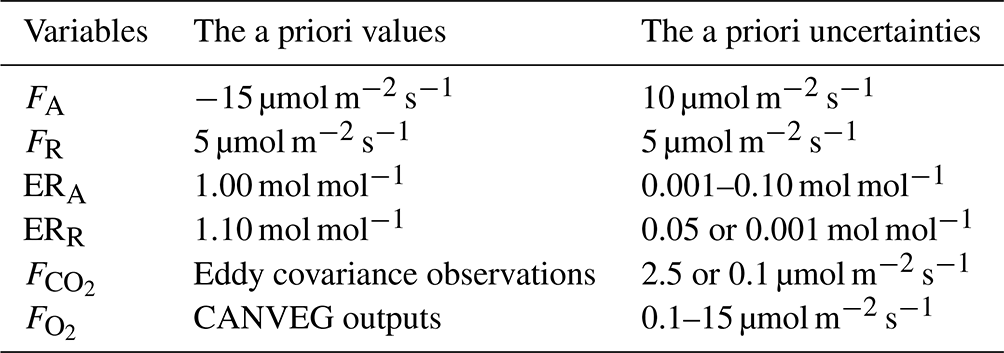
We evaluated the a posteriori uncertainties of partitioned photosynthetic fluxes on a typical day during summer (4 July 2012) with assigned a priori uncertainties. The a priori uncertainty of gross assimilation (${\mathit{\sigma }}_{F_{\mathrm{A}}^b}$) was set to 10 µmol m⁻² s⁻¹ and of ecosystem respiration (${\mathit{\sigma }}_{F_{\mathrm{R}}^b}$) to 5 µmol m⁻² s⁻¹, following Ogee et al. (2004) assuming less constraint on a posteriori results (Table 2). The uncertainty of the net CO₂ fluxes (${\mathit{\sigma }}_{F_{{\mathrm{CO}}_{\mathrm{2}}}}$) was derived from Mann and Lenschow's model (Lenschow et al., 1994) and calculated for our site to be 2.5 µmol m⁻² s⁻¹ (Braden-Behrens et al., 2019). We also examined if ${\mathit{\sigma }}_{F_{\mathrm{A}}}$ could be reduced if more accurate net CO₂ fluxes were measured (${\mathit{\sigma }}_{F_{{\mathrm{CO}}_{\mathrm{2}}}}=\mathrm{0.5}$ µmol m⁻² s⁻¹).

The uncertainty of measured ecosystem O₂ fluxes (${\mathit{\sigma }}_{F_{{\mathrm{O}}_{\mathrm{2}}}}$) is unknown to us. Consequently, we used the results from the flux-gradient method evaluation (Sect. 2.4.). In order to clearly quantify the effect of ${\mathit{\sigma }}_{F_{{\mathrm{O}}_{\mathrm{2}}}}$ and ${\mathit{\sigma }}_{{\mathrm{ER}}_{\mathrm{A}}}$ on flux-partitioning precision, we defined a ${\mathit{\sigma }}_{F_{{\mathrm{O}}_{\mathrm{2}}}}$ series ranging from 0.1 to 15 µmol m⁻² s⁻¹, representing the 90 % quantile of random Δo measurement uncertainty (see Sect. 2.4.), and a series of ${\mathit{\sigma }}_{{\mathrm{ER}}_{\mathrm{A}}^b}$ ranging from 0.001 to 0.1 mol mol⁻¹. ${\mathit{\sigma }}_{{\mathrm{ER}}_{\mathrm{R}}^b}$ was fixed to either 0.05 or 0.001 mol mol⁻¹.

Moreover, we assessed the impact of the model parameters ER_A, ER_stem and ER_soil on the source-partitioning results by changing each by ± 10 % and by estimating the absolute change in the a posteriori ${\mathit{\sigma }}_{F_{\mathrm{A}}}$.

3 Results

3.1 Model performance

The model generally showed similar performance for $F_{{\mathrm{CO}}_{\mathrm{2}}}$, H and LE during both calibration and validation (Fig. 2), indicating robust model behavior as a multilayer canopy flux simulator. The model validation for $F_{{\mathrm{CO}}_{\mathrm{2}}}$ (R²=0.82, slope of 1.016) was generally better than for H (R²=0.7, slope of 0.879) and LE (R²=0.77, slope of 1.02) (Fig. 2b, d and f). The disagreement between modeled and measured $F_{{\mathrm{CO}}_{\mathrm{2}}}$ indicated some uncertainties in the parameters for soil and stem respiration, as well as phenology, in the model equations. The similar scale but opposite sign of y intercepts for H and LE calibration simulations (Fig. 2c and e) indicated underestimation in H and the same amount of overestimation in LE. The slopes deviating from 1 for H and LE could come from a non-closure of the energy balance in the eddy covariance observations.

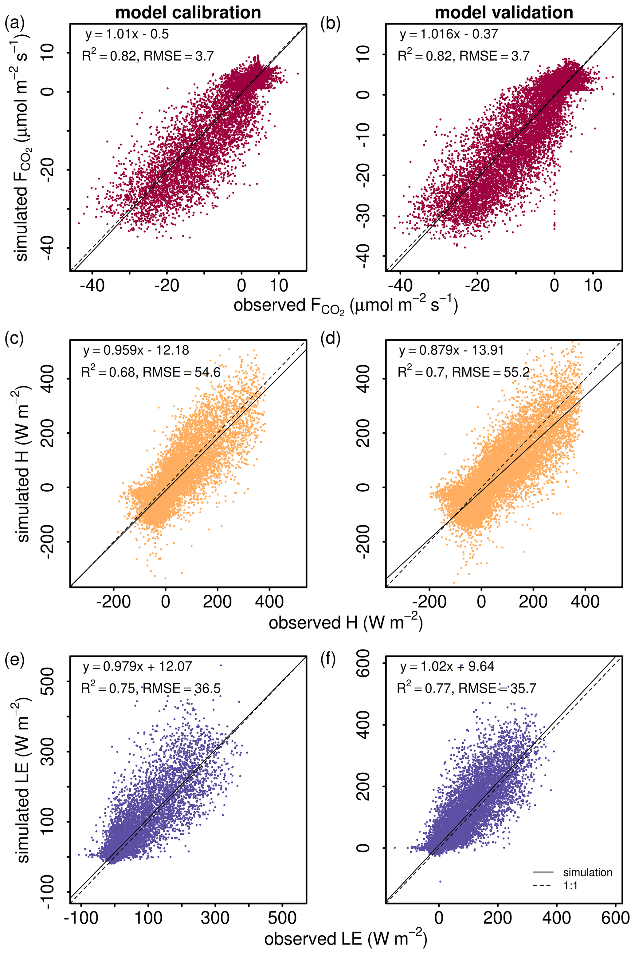
Figure 2 Comparison of (a, b) net ecosystem CO₂ flux ($F_{{\mathrm{CO}}_{\mathrm{2}}}$), (c, d) sensible heat flux (H), and (e, f) latent heat flux (LE) from 2012–2016 between model simulations (y axes) and eddy covariance observations (x axes). The left column shows all hourly data points for the calibration period (2012–2013), and the right column shows all hourly data points for the validation period (2014–2016). The linear regression line function, coefficient of determination (R²) and the root mean square error (RMSE) are included in each panel. The dashed lines are the 1:1 lines.

Due to potential variations in the ER model parameters (which were here taken from literature), we conducted a sensitivity analysis to show how these parameters affected the modeled $F_{{\mathrm{O}}_{\mathrm{2}}}$. If ER_A was increased or decreased by 10 %, the modeled $F_{{\mathrm{O}}_{\mathrm{2}}}$ sum of the entire study period increased or decreased on average by 20.3 % correspondingly. Similarly, a change by plus or minus 10 % increments in ER_soil and ER_stem caused the $F_{{\mathrm{O}}_{\mathrm{2}}}$ sum to decrease or increase by 8.6 % and 1.7 %, respectively. These results directly follow Eq. (1), where the derivative with respect to a specific ER gives the corresponding flux in percent. Oxygen fluxes were hence most sensitive to the ER of the largest carbon fluxes.

3.2 Temporal dynamics of O₂ : CO₂ exchange ratios

The median of the hourly ecosystem O₂ : CO₂ exchange ratio (ER_eco) throughout the simulation period (2012–2016) was 1.08 mol mol⁻¹, where the annual medians did not differ between years. The annual mean ER_eco ranged from 1.06 to 1.12 mol mol⁻¹ across the 5 years. Hourly ER_eco also varied seasonally and within the diel course, as shown as an example for the year 2012 in Fig. 3a. During the non-growing season, ER_eco values were constrained between 1.04 and 1.10 mol mol⁻¹, representing a mixture of the prevailing stem and soil respiration processes. During the growing season, ER_eco was close to 1.00 mol mol⁻¹ during daylight hours due to the dominance of photosynthetic processes and sometimes even smaller than 1.00 mol mol⁻¹ when daytime $F_{{\mathrm{O}}_{\mathrm{2}}}$ was smaller than daytime $F_{{\mathrm{CO}}_{\mathrm{2}}}$. This could occur with ER_A= 1.00 mol mol⁻¹ and ER_stem, ER_soil and ER_rd >1.00 mol mol⁻¹ (following Eq. 1) when more O₂ was consumed than CO₂ released for the respiratory fluxes, and thus the magnitude of net $F_{{\mathrm{O}}_{\mathrm{2}}}$ decreased. During nighttime in the growing season, ER_eco was > 1.00 mol mol⁻¹, representing a mixture of stem, soil and leaf dark respiration. For transition periods (sunrise and sunset), with flux magnitudes close to zero, ER_eco values were very high, owing to very small $F_{{\mathrm{CO}}_{\mathrm{2}}}$. Because ER_eco is a ratio, values could get extremely large and approach infinity as $F_{{\mathrm{CO}}_{\mathrm{2}}}$ approaches zero. However, since corresponding $F_{{\mathrm{O}}_{\mathrm{2}}}$ values were also very low, these ER_eco values had very little effect on median and mean ER_eco of the overall ecosystem over a longer time period.

Within the sensitivity analysis, the initial annual median ER_eco of 1.08 mol mol⁻¹ changed only by up to 0.02 mol mol⁻¹ due to the change in ER_A or ER_stem by ± 10 %. Increasing or decreasing ER_soil had the largest impact, where median ER_eco increased or decreased to 1.00 or 1.17 mol mol⁻¹, respectively. Also here, the interannual difference between years was very small. A similar pattern could be found for the annual mean ER_eco, which varied between 1.04 and 1.15 mol mol⁻¹ depending on ER_A and ER_stem and varied even between 1.00 and 1.24 mol mol⁻¹ due to ER_soil.

The median and mean of hourly O₂ : CO₂ net assimilation ratio (ER_An) were 0.99 and 0.97 mol mol⁻¹, respectively, for all growing seasons during the simulation period and did not vary between years. In the sensitivity analysis, ER_An was only slightly impacted by changes in the model parameter of ER_A (ER_stem and ER_soil had no impact). Again, the seasonal and diel variations in ER_An in the year 2012 of the original simulation are shown in Fig. 3b as an example. During nighttime, ER_An was equivalent to ER_rd and thus also dependent on T_leaf (Fig. 1b). With low T_leaf at the beginning or end of the growing season, ER_An was often smaller than 0.90 mol mol⁻¹. During daytime, when the magnitude of F_A was usually much larger than the magnitude of the opposing flux F_rd, ER_An was negatively correlated to T_leaf. Note that F_rd and ER_rd responded differently to T_leaf; that is, F_rd was a fraction of V_cmax, which had an optimal temperature at 27 ^∘C (Table 1), while ER_rd was positively correlated with T_leaf (Fig. 1b). Consequently, during periods with high T_leaf and low irradiation, F_rd was small, but ER_rd was large, and the magnitude of the O₂ flux of leaf respiration was larger than the magnitude of the CO₂ flux with $|-F_{\mathrm{rd}}\cdot$ ER${}_{\mathrm{rd}}\left|\mathit{>}\right|F_{\mathrm{rd}}|$. Moreover, $|-F_{\mathrm{A}}\cdot$ ER_A| and $\left|F_{\mathrm{A}}\right|$ were small with ER_A=1.00 mol mol⁻¹. It followed that under these conditions and given model implementation, ER_An described the ratio of O₂ uptake and CO₂ uptake (both fluxes with the same sign), when more O₂ was consumed due to leaf dark respiration than released by assimilation ($|-F_{\mathrm{rd}}\cdot$ ER${}_{\mathrm{rd}}\left|\mathit{>}\right|-F_{\mathrm{A}}\cdot$ ER_A|). In addition, because values of F_A were below zero and values of F_rd were greater than zero, values of ER_An (Eq. 3) laid mostly not between ER_A and ER_rd. Similar to ER_eco, high variations in ER_An were usually found during transition periods with low flux magnitudes.

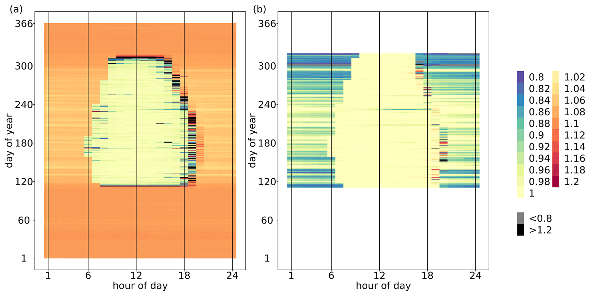
Figure 3 Temporal variations in (a) the exchange ratio of net ecosystem fluxes (ER_eco, mol mol⁻¹) and (b) the exchange ratio of net assimilation (ER_An, mol mol⁻¹) by hour of day and day of year in 2012. The exchange ratios were calculated as the ratio of the hourly $F_{{\mathrm{O}}_{\mathrm{2}}}$ and $F_{{\mathrm{CO}}_{\mathrm{2}}}$ (including storage terms) summed up over the entire canopy height. As a guide, 1 July is day 183.

3.3 Vertical profiles of O₂ : CO₂ flux and mole fraction ratios

The vertical profiles of ER_eco and ER_conc differed temporally and spatially. Figure 4 shows the diel vertical profiles of ER${}_{\mathrm{eco}}^z$ and ER${}_{\mathrm{conc}}^z$ averaged over all growing seasons from 2012–2016 (between leaf_out and leaf_{fall_complete}). The mean diel ER${}_{\mathrm{eco}}^z$ ranged from 0.985 to 1.10 mol mol⁻¹ (Fig. 4a). ER${}_{\mathrm{eco}}^z$ at the ground and bottom layers ($z/\mathrm{ht}\le \mathrm{0.35}$) showed very little variability across the day, reflecting the dominance of stem and soil respiration with fixed values of ER_soil and ER_stem (Fig. 4a). The upper levels of the canopy showed ER${}_{\mathrm{eco}}^z$ between 0.99 and 1.04 mol mol⁻¹ during the daylight period (06:00 to 20:00; all times are UTC + 1) due to the dominating fluxes of assimilation and stem respiration. The leaf dark respiration did not have a large impact on averaged daytime ER${}_{\mathrm{eco}}^z$. Moreover, the defined LAI and WAI distributions (Fig. 1a) were represented in the vertical profile of ER${}_{\mathrm{eco}}^z$, whereas the top canopy contained a larger proportion of sunlit leaves ($z/\mathrm{ht}\mathit{>}\mathrm{0.75}$) than the middle part (0.35 < $z/\mathrm{ht}$ < 0.75). Hence, ER${}_{\mathrm{eco}}^z$ in the top canopy was influenced more by fluxes of assimilation in daytime hours and was close to 1.00 mol mol⁻¹. Between $z/\mathrm{ht}=\mathrm{0.3}$ and $z/\mathrm{ht}=\mathrm{0.5}$, ER${}_{\mathrm{eco}}^z$ was larger than 1.06 mol mol⁻¹ during daytime due to higher respiratory processes than assimilation affected by low radiation and relatively high temperatures. The ER${}_{\mathrm{eco}}^z$ during nighttime (approximately before 06:00 and after 20:00) of the upper and middle canopy was usually larger than 1.04 mol mol⁻¹ due to respiratory fluxes.

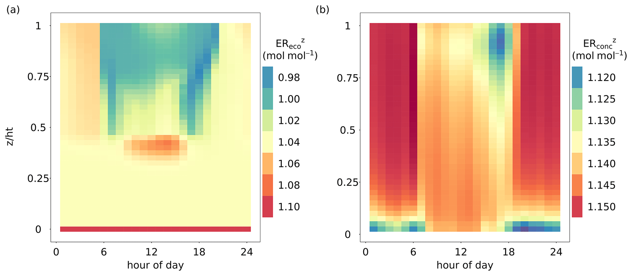
Figure 4 Comparison of the diel dynamics of the height-dependent O₂ : CO₂ flux and mole fraction ratios averaged over all growing seasons (day of year 110 to 320) from 2012–2016. (a) Vertical profile of the O₂ : CO₂ flux ratio inside the canopy (ER${}_{\mathrm{eco}}^z$, mol mol⁻¹), including the whole canopy domain and the soil component ($z/\mathrm{ht}=\mathrm{0}$). (b) Vertical profile of the O₂ : CO₂ mole fraction ratio inside the canopy (ER${}_{\mathrm{conc}}^z$, mol mol⁻¹), including the whole canopy domain. The exchange ratios for specific canopy heights were derived as the slope of linear regressions fitted to O₂ and CO₂ fluxes or dry-air mole fractions of multiple simulated time steps for each canopy layer.

The mean diel ER${}_{\mathrm{conc}}^z$ showed relatively small variations ranging from 1.115 to 1.15 mol mol⁻¹ (Fig. 4b) and thus closely matched the prescribed atmospheric O₂ : CO₂ mole fraction slope of 1.15 (Table 1). Especially during nighttime (before 06:00 and after 20:00), ER${}_{\mathrm{conc}}^z$ was mainly driven by the atmospheric O₂ and CO₂ background levels. However, bottom layers showed slightly lower values of ER${}_{\mathrm{conc}}^z$, down to 1.12 mol mol⁻¹, owing to an accumulation of CO₂ close to the soil surface produced by soil respiration and low turbulence. During daytime, the canopy air column was well mixed due to stronger turbulence. Nevertheless, ER${}_{\mathrm{conc}}^z$ values were slightly lower in the top canopy layers towards late afternoon and sunset, caused by prevailing canopy respiration.

3.4 Evaluation of the flux-gradient method to obtain O₂ fluxes

The vertical profiles of air temperature, water vapor, CO₂ and O₂ mole fractions were modeled for the entire CANVEG domain including 40 canopy layers and 80 atmosphere layers above the canopy. Figure 5 shows examples of vertical profiles for 12:00 to 13:00 (daytime) and 23:00 to 00:00 (nighttime) on 4 July 2012, an arbitrarily chosen sunny day. Generally, during daytime the vertical profiles within the canopy (Fig. 5a and c) were mostly induced by radiative transfer, leaf photosynthesis, transpiration and autotrophic respiration, which were influenced by the vertical LAI and WAI distributions (Fig. 1a). Furthermore, soil evaporation and respiration resulted in higher water vapor and CO₂ mole fractions close to the soil surface. For the layers above the canopy ($z/\mathrm{ht}\mathit{>}\mathrm{1}$), the profiles changed monotonically. Daytime O₂ and CO₂ profiles (Fig. 5c) showed a mirrored shape because the O₂ and CO₂ fluxes were contributing inversely to the atmospheric mole fractions. Nighttime water vapor and CO₂ profiles (Fig. 5d and d) showed a continuous decrease with height and the O₂ profile a continuous increase due to the dominance of soil evaporation and soil, with stem and leaf respiration in the lower layers being a sink for O₂. During nighttime, air temperature (Fig. 5b) was slightly lower at the canopy top than inside the canopy due to higher energy loss by the emission of longwave radiation.

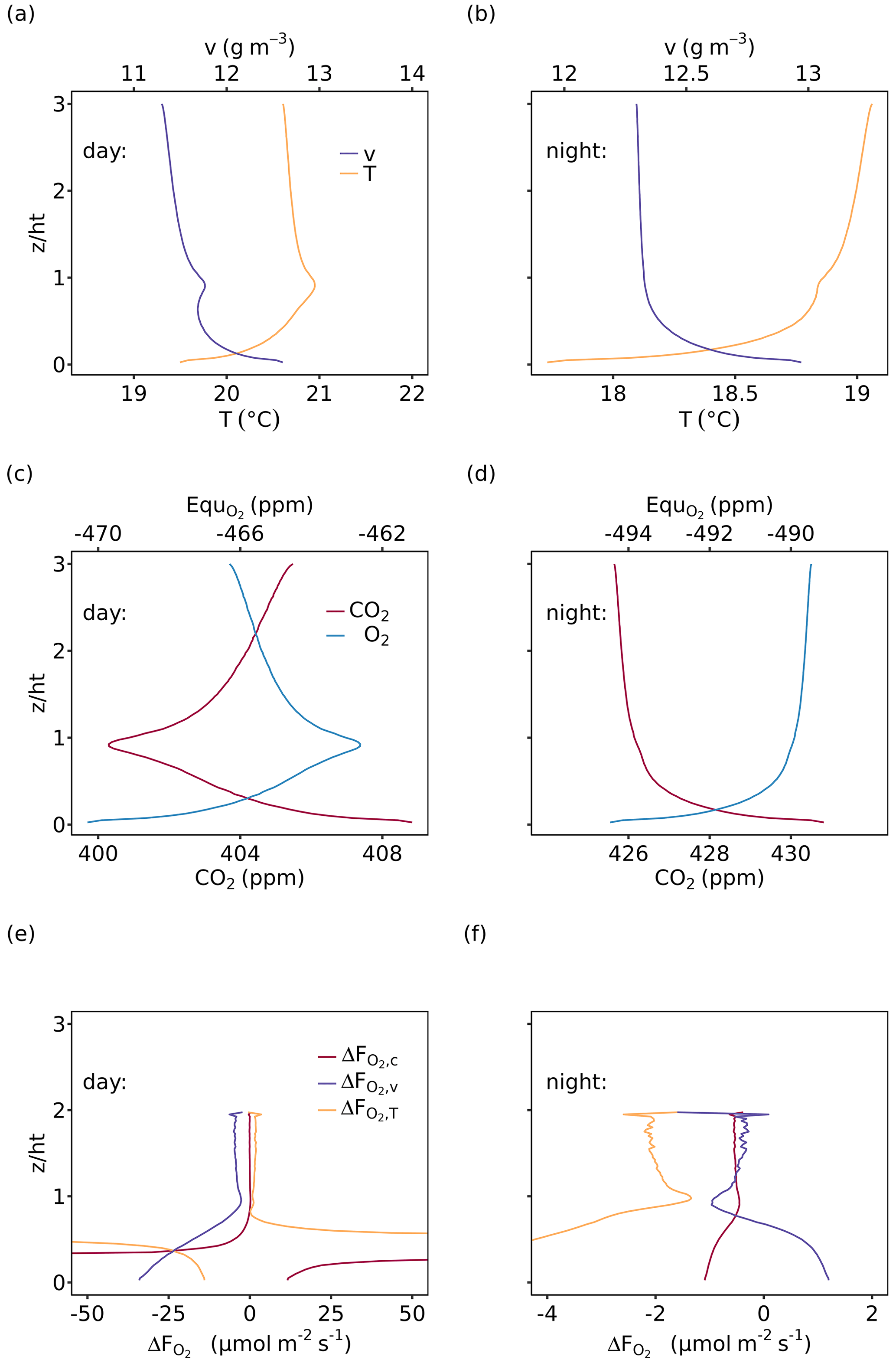
Figure 5 Vertical profiles of (a, b) air temperature (T) and water vapor (v) and (c, d) CO₂ and O₂ mole fractions of the entire model domain, where O₂ mole fractions are shown as the difference from 209 750 ppm (${\mathrm{Equ}}_{{\mathrm{O}}_{\mathrm{2}}}$, 209 750 ppm was derived as the intercept of the relationship between measured atmospheric O₂ and CO₂ mole fractions; see Table 1). (e, f) $\mathrm{\Delta }{F}_{{\mathrm{O}}_{\mathrm{2}},(\mathrm{c},\mathrm{T},\mathrm{v})}$ that resulted from Eq. (7) (Sect. 2.4). The left panels (a), (c) and (e) show mean profiles for 12:00 to 13:00 (daytime) and the right panels (c), (d) and (f) for 23:00 to 00:00 (nighttime), all for 4 July 2012. The flux-gradient method was applied for the gradients between a top measurement height at $z/\mathrm{ht}$ = 2 and each layer below and is based on profiles and fluxes of CO₂, H and LE ($\mathrm{\Delta }{F}_{{\mathrm{O}}_{\mathrm{2}},\mathrm{c}}$, $\mathrm{\Delta }{F}_{{\mathrm{O}}_{\mathrm{2}},\mathrm{T}}$ and $\mathrm{\Delta }{F}_{{\mathrm{O}}_{\mathrm{2}},\mathrm{v}}$).

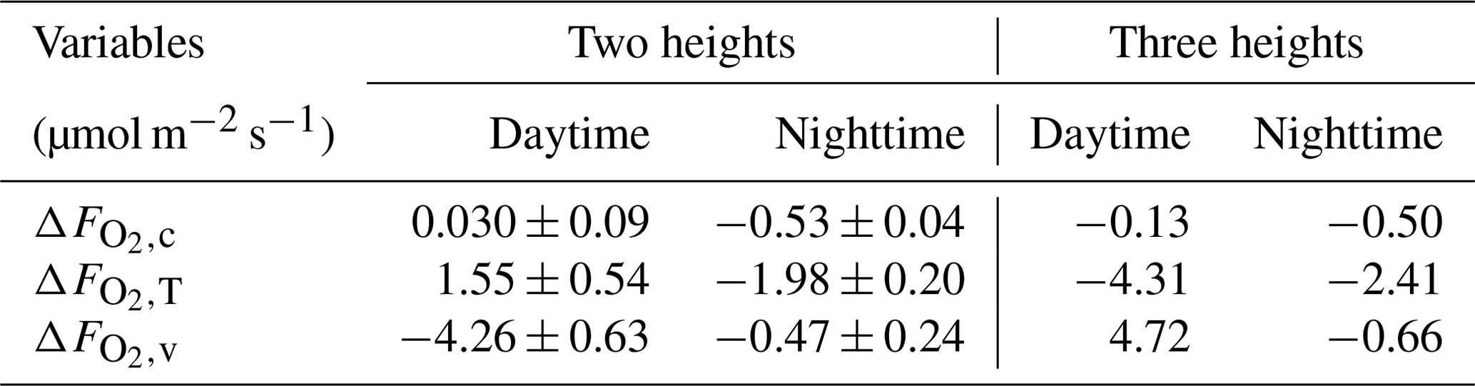
Based on these modeled vertical profiles and the corresponding flux ($F_{{\mathrm{CO}}_{\mathrm{2}}}$, H or LE, respectively), O₂ fluxes were calculated with the flux-gradient method and compared to the modeled O₂ fluxes from CANVEG, both corrected for the storage term. So in the following we always describe the ecosystem fluxes (turbulent fluxes plus storage terms). Figure 5e and f show the difference between the various flux-gradient methods derived and modeled $F_{{\mathrm{O}}_{\mathrm{2}}}$ ($\mathrm{\Delta }{F}_{{\mathrm{O}}_{\mathrm{2}},(\mathrm{c},\mathrm{T},\mathrm{v})}$; Eq. 7) for the respective simulation hours, when the scalar gradients were derived from two heights (Sect. 2.4). An $F_{{\mathrm{O}}_{\mathrm{2}}}$ estimate and a $\mathrm{\Delta }{F}_{{\mathrm{O}}_{\mathrm{2}},(\mathrm{c},\mathrm{T},\mathrm{v})}$ value were obtained for each layer. Generally, $\mathrm{\Delta }{F}_{{\mathrm{O}}_{\mathrm{2}}}$ derived with the flux-gradient method based on the CO₂ profile ($\mathrm{\Delta }{F}_{{\mathrm{O}}_{\mathrm{2}},\mathrm{c}}$) was lower than $\mathrm{\Delta }{F}_{{\mathrm{O}}_{\mathrm{2}}}$ derived from the temperature and water vapor profile ($\mathrm{\Delta }{F}_{{\mathrm{O}}_{\mathrm{2}},\mathrm{T}}$, $\mathrm{\Delta }{F}_{{\mathrm{O}}_{\mathrm{2}},\mathrm{v}}$; Fig. 5e and f). For daytime conditions (Fig. 5e), the mean $\mathrm{\Delta }{F}_{{\mathrm{O}}_{\mathrm{2}},\mathrm{c}}$, $\mathrm{\Delta }{F}_{{\mathrm{O}}_{\mathrm{2}},\mathrm{T}}$ and $\mathrm{\Delta }{F}_{{\mathrm{O}}_{\mathrm{2}},\mathrm{v}}$ above the canopy were 0.030 ± 0.09, 1.55 ± 0.54 and −4.26 ± 0.63 µmol m⁻² s⁻¹, respectively (Table 3). There was little vertical variation in $\mathrm{\Delta }{F}_{{\mathrm{O}}_{\mathrm{2}},(\mathrm{c},\mathrm{T},\mathrm{v})}$ above the canopy for nighttime (Fig. 5f). Here, the mean $\mathrm{\Delta }{F}_{{\mathrm{O}}_{\mathrm{2}},\mathrm{c}}$, $\mathrm{\Delta }{F}_{{\mathrm{O}}_{\mathrm{2}},\mathrm{T}}$ and $\mathrm{\Delta }{F}_{{\mathrm{O}}_{\mathrm{2}},\mathrm{v}}$ were −0.53 ± 0.04, −1.98 ± 0.20 and −0.47 ± 0.24 µmol m⁻² s⁻¹, respectively. By applying the three-height flux-gradient method based on Faassen et al. (2023), $\mathrm{\Delta }{F}_{{\mathrm{O}}_{\mathrm{2}}}$ for the daytime hours had a similar magnitude for $\mathrm{\Delta }{F}_{{\mathrm{O}}_{\mathrm{2}},\mathrm{c}}$ at −0.13 µmol m⁻² s⁻¹ and for $\mathrm{\Delta }{F}_{{\mathrm{O}}_{\mathrm{2}},\mathrm{v}}$ at −4.31 µmol m⁻² s⁻¹ and was larger for $\mathrm{\Delta }{F}_{{\mathrm{O}}_{\mathrm{2}},\mathrm{T}}$ at 4.72 µmol m⁻² s⁻¹. The corresponding nighttime $\mathrm{\Delta }{F}_{{\mathrm{O}}_{\mathrm{2}},\mathrm{c}}$, $\mathrm{\Delta }{F}_{{\mathrm{O}}_{\mathrm{2}},\mathrm{T}}$ and $\mathrm{\Delta }{F}_{{\mathrm{O}}_{\mathrm{2}},\mathrm{v}}$ derived from the three-height flux-gradient method were −0.50, −2.41 and −0.66 µmol m⁻² s⁻¹, indicating the similar $\mathrm{\Delta }{F}_{{\mathrm{O}}_{\mathrm{2}},\mathrm{c}}$ and $\mathrm{\Delta }{F}_{{\mathrm{O}}_{\mathrm{2}},\mathrm{v}}$ but a larger magnitude of $\mathrm{\Delta }{F}_{{\mathrm{O}}_{\mathrm{2}},\mathrm{T}}$ than with the two-height flux-gradient method.

Table 3 Difference between the $F_{{\mathrm{O}}_{\mathrm{2}}}$ estimations derived by the flux-gradient method ($F_{{\mathrm{O}}_{\mathrm{2}},(\mathrm{c},\mathrm{T},\mathrm{v})}^{\sim }$, based on $F_{{\mathrm{CO}}_{\mathrm{2}}}^{\sim }$, H^∼ or LE^∼ and their respective vertical scalar profile) and by model simulations ($F_{{\mathrm{O}}_{\mathrm{2}},\mathrm{CANVEG}}^{\sim }$) for above-canopy fluxes and for day- and nighttime individually. Results of the two-height approach are shown as the mean and standard deviation of flux gradients derived between $z/\mathrm{ht}$ = 2 and each layer below or above the canopy. Also results of the three-height approach are shown, where the flux gradient was derived between three fixed heights ($z/\mathrm{ht}$ = 1.05, 1.45 and 2 with ht = 37.5 m).

The $\mathrm{\Delta }{F}_{{\mathrm{O}}_{\mathrm{2}},(\mathrm{c},\mathrm{T},\mathrm{v})}$ within the canopy during daytime increased and was highly variable for all three methods due to the presence of sources and sinks, as well as nonlinearity of the gradients (Fig. 5e). $\mathrm{\Delta }{F}_{{\mathrm{O}}_{\mathrm{2}},\mathrm{c}}$ and $\mathrm{\Delta }{F}_{{\mathrm{O}}_{\mathrm{2}},\mathrm{T}}$ showed hyperbolic shapes with very low (< −50 µmol m⁻² s⁻¹) and high values (> 50 µmol m⁻² s⁻¹), where the CO₂ dry-air mole fractions or the temperatures, respectively, were very close to the conditions at the top measurement height, and so the gradients were very small. The sudden jumps from large positive to large negative values were caused by the change in signs of Δc and ΔT.

To guarantee a large gradient, the heights with $z/\mathrm{ht}=\mathrm{2}$ and $z/\mathrm{ht}=\mathrm{1.05}$ were used in inferring $F_{{\mathrm{O}}_{\mathrm{2}}}$ from vertical CO₂, temperature and water vapor gradients for the following analysis. Figure 6a, b and c show the median diel courses of $\mathrm{\Delta }{F}_{{\mathrm{O}}_{\mathrm{2}},\mathrm{c}}$, $\mathrm{\Delta }{F}_{{\mathrm{O}}_{\mathrm{2}},\mathrm{T}}$ and $\mathrm{\Delta }{F}_{{\mathrm{O}}_{\mathrm{2}},\mathrm{v}}$ for all growing seasons from 2012–2016. Assuming that with these heights the gradients were large enough, the inferred $F_{{\mathrm{O}}_{\mathrm{2}}}$ agreed well with modeled $F_{{\mathrm{O}}_{\mathrm{2}}}$ for $\mathrm{\Delta }{F}_{{\mathrm{O}}_{\mathrm{2}},\mathrm{c}}$ throughout the median diel course, ranging from −0.45 to −0.15 µmol m⁻² s⁻¹ (Fig. 6a). The medians of $\mathrm{\Delta }{F}_{{\mathrm{O}}_{\mathrm{2}},\mathrm{T}}$ and $\mathrm{\Delta }{F}_{{\mathrm{O}}_{\mathrm{2}},\mathrm{v}}$ indicated that $F_{{\mathrm{O}}_{\mathrm{2}},\mathrm{T}}$ was overestimated by up to 1.59 µmol m⁻² s⁻¹ and $F_{{\mathrm{O}}_{\mathrm{2}},\mathrm{v}}$ underestimated by up to 5.43 µmol m⁻² s⁻¹ during daytime hours (Fig. 6b and c). The standard deviations of $\mathrm{\Delta }{F}_{{\mathrm{O}}_{\mathrm{2}},(\mathrm{c},\mathrm{T},\mathrm{v})}$ reflected the diel variation in turbulent conditions and vertical gradients, which were also dependent on the eddy diffusivity. The nighttime standard deviation of $\mathrm{\Delta }{F}_{{\mathrm{O}}_{\mathrm{2}},\mathrm{v}}$ was relatively large but smaller for $\mathrm{\Delta }{F}_{{\mathrm{O}}_{\mathrm{2}},\mathrm{T}}$. The latter produced more outliers during daytime, especially during times of sunrise and sunset. The standard deviation of $\mathrm{\Delta }{F}_{{\mathrm{O}}_{\mathrm{2}},\mathrm{c}}$ was relatively low and usually < 10 µmol m⁻² s⁻¹ across all times of the day except at 08:00, 12:00 and 19:00 (Fig. 6a).

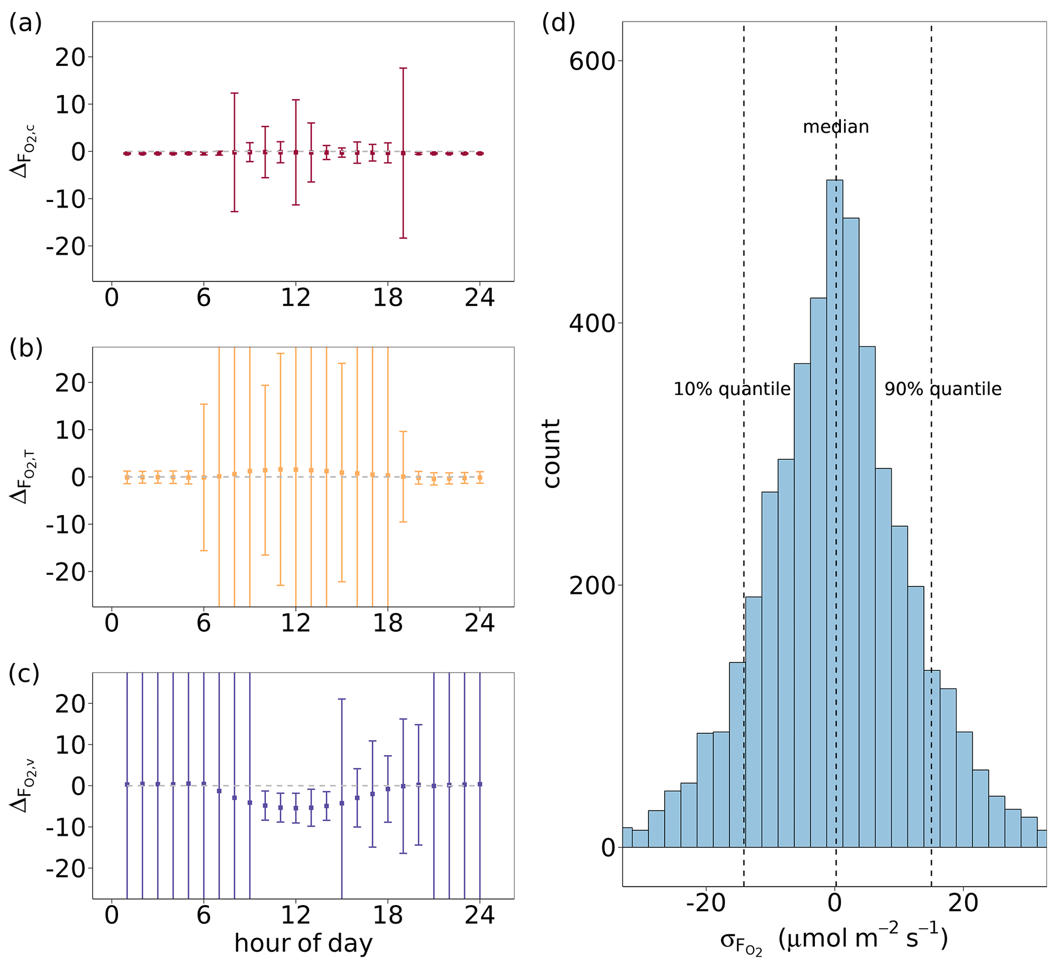
Figure 6 (a, b, c) Median diel cycles of the differences between O₂ fluxes derived by the flux-gradient method and by CANVEG simulation ($\mathrm{\Delta }{F}_{{\mathrm{O}}_{\mathrm{2}},(\mathrm{c},\mathrm{T},\mathrm{v})}$) for all growing seasons from 2012–2016. The flux-gradient method was applied for the gradients between $z/\mathrm{ht}$ = 2 and $z/\mathrm{ht}$ = 1.05 and is based on profiles and fluxes of (a) CO₂, (b) H and (c) LE ($\mathrm{\Delta }{F}_{{\mathrm{O}}_{\mathrm{2}},\mathrm{c}}$, $\mathrm{\Delta }{F}_{{\mathrm{O}}_{\mathrm{2}},\mathrm{T}}$ and $\mathrm{\Delta }{F}_{{\mathrm{O}}_{\mathrm{2}},\mathrm{v}}$). The error bars indicate the standard deviation of $\mathrm{\Delta }{F}_{{\mathrm{O}}_{\mathrm{2}},(\mathrm{c},\mathrm{T},\mathrm{v})}$ by hour. (d) Histogram of uncertainties in $F_{{\mathrm{O}}_{\mathrm{2}}}$ (${\mathit{\sigma }}_{F_{{\mathrm{O}}_{\mathrm{2}}}}$) derived by the flux-gradient method based on CO₂ profiles and fluxes, in which a random uncertainty in O₂ mole fractions (Δo) was included. The uncertainty in Δo followed a normal distribution with a mean of 0 and a standard deviation of 0.7 ppm (Pickers et al., 2017). In order to include daytime hours with an active canopy for the estimation of ${\mathit{\sigma }}_{F_{{\mathrm{O}}_{\mathrm{2}}}}$, Δo ≥ 1 ppm was used as a filter, assuming higher-oxygen dry-air mole fractions close to the canopy than in the top domain layers.

The above analysis evaluated the flux-gradient method solely regarding the characteristics and dynamics of various scalar gradients. Moreover, accurate and precise measurements of the scalars are also necessary for the satisfactory performance of this method. We added a random uncertainty to our modeled O₂ mole fractions to simulate gradient measurements with the current instrument uncertainty (Δo in Eq. 6). Figure 6d shows the distribution of the differences (${\mathit{\sigma }}_{F_{{\mathrm{O}}_{\mathrm{2}}}}$) between the $F_{{\mathrm{O}}_{\mathrm{2}}}$ estimates based on the flux-gradient method including a random measurement uncertainty in Δo or not. For this analysis, only hourly time steps within all growing seasons from 2012–2016 were chosen with Δo ≥ 1 ppm, when O₂ mole fractions increased with decreasing height above the canopy due to prevailing gross assimilation over respirations during daytime. The median of resulting ${\mathit{\sigma }}_{F_{{\mathrm{O}}_{\mathrm{2}}}}$ was 0.20 µmol m⁻² s⁻¹ and thus very close to zero. Here, we extracted the 10 % and 90 % quantile of ${\mathit{\sigma }}_{F_{{\mathrm{O}}_{\mathrm{2}}}}=-\mathrm{14.2}$ and 14.5 µmol m⁻² s⁻¹. Thus, we used 15 µmol m⁻² s⁻¹ as the upper limit of ${\mathit{\sigma }}_{F_{{\mathrm{O}}_{\mathrm{2}}}}$ in the evaluation of the flux-partitioning approach (Sect. 3.5).

3.5 Uncertainties in partitioning net ecosystem CO₂ fluxes based on O₂ fluxes

For the test day from 07:00 to 19:00 on 4 July 2012, model output of hourly $F_{{\mathrm{O}}_{\mathrm{2}}}$ was used to derive the main CO₂ flux components. The a posteriori uncertainties of the partitioned fluxes of gross assimilation (${\mathit{\sigma }}_{F_{\mathrm{A}}}$) decreased significantly with decreasing uncertainties of ${\mathit{\sigma }}_{{\mathrm{ER}}_{\mathrm{A}}}$ and ${\mathit{\sigma }}_{F_{{\mathrm{O}}_{\mathrm{2}}}}$, indicating the importance of reducing errors in ER and O₂ flux measurements (Fig. 7). The a priori uncertainties had strong effects on a posteriori uncertainties because a large ${\mathit{\sigma }}_{F_{\mathrm{A}}^b}$ allowed large $\mathrm{|}{F}_{\mathrm{A}}-F_{\mathrm{A}}^b\mathrm{|}$ to reach a minimum J value and vice versa (Eq. 8). Without the constraints of a priori uncertainties (Fig. 7a), ${\mathit{\sigma }}_{F_{\mathrm{A}}}$ reached 193 µmol m⁻² s⁻¹ at its maximum and then reduced with smaller ${\mathit{\sigma }}_{F_{{\mathrm{O}}_{\mathrm{2}}}}$ and ${\mathit{\sigma }}_{{\mathrm{ER}}_{\mathrm{A}}}$ to 28 µmol m⁻² s⁻¹, which was still larger than the a priori value (Table 2). If a priori uncertainties (${\mathit{\sigma }}_{F_{\mathrm{A}}^b}$, ${\mathit{\sigma }}_{F_{\mathrm{R}}^b}$, ${\mathit{\sigma }}_{{\mathrm{ER}}_{\mathrm{A}}^b}$, ${\mathit{\sigma }}_{{\mathrm{ER}}_{\mathrm{R}}^b}$) were included (Fig. 7b and c), ${\mathit{\sigma }}_{F_{\mathrm{A}}}$ was much lower. When assuming an uncertainty for the net CO₂ fluxes (${\mathit{\sigma }}_{F_{{\mathrm{CO}}_{\mathrm{2}}}}$) of 2.5 µmol m⁻² s⁻¹, ${\mathit{\sigma }}_{F_{\mathrm{A}}}$ showed very little variation and ranged between 4.74 and 4.88 µmol m⁻² s⁻¹, remaining close to the minimum of the chosen a priori uncertainty in F_A and F_R (Fig. 7b). When assuming more accurate $F_{{\mathrm{CO}}_{\mathrm{2}}}$ and ER_R measurements with ${\mathit{\sigma }}_{F_{{\mathrm{CO}}_{\mathrm{2}}}}=\mathrm{0.5}$ µmol m⁻² s⁻¹ and ${\mathit{\sigma }}_{{\mathrm{ER}}_{\mathrm{R}}}=\mathrm{0.001}$ mol mol⁻¹, ${\mathit{\sigma }}_{F_{\mathrm{A}}}$ was reduced to a minimum of 1.43 µmol m⁻² s⁻¹ (Fig. 7c). A moderate level of a priori uncertainties in O₂ fluxes and ER_A (bold black lines in Fig. 7c) resulted in ${\mathit{\sigma }}_{F_{\mathrm{A}}}=\mathrm{4.48}$ µmol m⁻² s⁻¹ for our test day. In this case, the partitioned F_A was 28.3 µmol m⁻² s⁻¹, which was about 6 % lower than the estimated gross assimilation obtained with the eddy covariance technique ($F_{\mathrm{A}}^b=\mathrm{30.2}$ µmol m⁻² s⁻¹). With regard to the sensitivity analysis, ${\mathit{\sigma }}_{F_{\mathrm{A}}}$ was only slightly impacted by ER_A. ${\mathit{\sigma }}_{F_{\mathrm{A}}}$ ranged from 1.42 to 4.83 µmol m⁻² s⁻¹ for the case of the lower a priori uncertainty (with ${\mathit{\sigma }}_{F_{{\mathrm{CO}}_{\mathrm{2}}}}=\mathrm{0.5}$ µmol m⁻² s⁻¹ and ${\mathit{\sigma }}_{{\mathrm{ER}}_{\mathrm{R}}}=\mathrm{0.001}$ mol mol⁻¹).

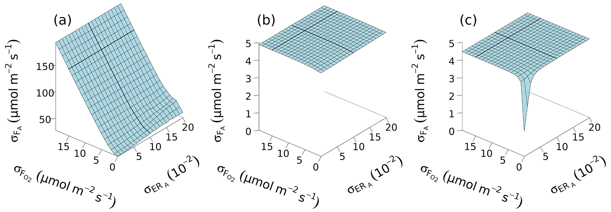
Figure 7 Uncertainty in partitioned gross assimilation CO₂ flux (F_A) determined from eddy covariance net ecosystem CO₂ flux ($F_{{\mathrm{CO}}_{\mathrm{2}}}$) with net ecosystem O₂ flux ($F_{{\mathrm{O}}_{\mathrm{2}}}$), O₂ : CO₂ ratio of gross assimilation (ER_A) and ecosystem respiration (ER_R) on 4 July 2012. (a) Optimized a posteriori uncertainty of F_A (${\mathit{\sigma }}_{F_{\mathrm{A}}}$) without a priori F_A values and uncertainties. (b) Optimized ${\mathit{\sigma }}_{F_A}$ including all of the a priori terms in the J function as written in Eq. (8), with a priori uncertainty of $F_{{\mathrm{CO}}_{\mathrm{2}}}$ (${\mathit{\sigma }}_{F_{{\mathrm{CO}}_{\mathrm{2}}}}$) = 2.5 µmol m⁻² s⁻¹ and a priori uncertainty of ER_R (${\mathit{\sigma }}_{{\mathrm{ER}}_{\mathrm{R}}^b}$) = 0.05 mol mol⁻¹. (c) Same cost function as for (b) but with ${\mathit{\sigma }}_{F_{{\mathrm{CO}}_{\mathrm{2}}}}=\mathrm{0.5}$ µmol m⁻² s⁻¹ and ${\mathit{\sigma }}_{{\mathrm{ER}}_{\mathrm{R}}^b}=$ 0.001 mol mol⁻¹. The bold black lines show the practical optimization test with ${\mathit{\sigma }}_{{\mathrm{ER}}_{\mathrm{A}}^b}$ and ${\mathit{\sigma }}_{F_{{\mathrm{O}}_{\mathrm{2}}}}$ around 0.01 mol mol⁻¹ and 15 µmol m⁻² s⁻¹, respectively (see Fig. 6d).

4 Discussions

4.1 Model setup and model performance

We added O₂ : CO₂ exchange ratios and O₂ flux processes into the one-dimensional, multilayer atmosphere–biosphere gas exchange model CANVEG. To represent natural atmosphere–ecosystem exchange satisfactorily, we first calibrated and validated the model based on eddy covariance CO₂ and energy flux observations from a temperate deciduous forest in Leinefelde, Germany, from 2012–2016. In a previous study, model performance was evaluated based on hourly CO₂, water vapor and energy fluxes in temperate oak forests (Baldocchi and Wilson, 2001). That evaluation, for hourly $F_{{\mathrm{CO}}_{\mathrm{2}}}$, yielded a slope of 1.09 of the regression between observations and simulation with R² = 0.82, which is comparable to our results (slope of 1.02 and R²=0.82; Fig. 2b). The model application in a deciduous temperate forest in central Germany (Knohl and Baldocchi, 2008) also showed a high match between hourly modeled and measured $F_{{\mathrm{CO}}_{\mathrm{2}}}$ (slope of 0.997, R² = 0.857). In addition, Hanson et al. (2004) compared the CANVEG model with seven other stand-level models where CANVEG performed very well (slope of 0.93, R²=0.82) based on simulated $F_{{\mathrm{CO}}_{\mathrm{2}}}$. In our study, the comparison between hourly LE simulation and observations obtained a regressed slope of 1.02 and R²=0.77 (Fig. 2f), indicating a better model performance than for daily evapotranspiration by Hanson et al. (2004) (slope of 1.17, R²=0.73). Knohl and Baldocchi (2008) found a slope of 0.926 and R²=0.825 for hourly LE simulation and a slope of 1.021 and R²=0.869 for hourly H simulation, indicating an underestimation of LE and a small overestimation of H. In our study, we observed an overestimation of LE and underestimation of H. The model performance (with regard to the slope, R² and RMSE) in the energy fluxes was generally lower than for CO₂ flux simulations because fitted parameters mainly affected the CO₂ fluxes and leaf assimilation (Table 1). By adjusting the assimilation rate, only transpiration was changed, which then had an impact on LE and H. The non-unity slope of H and LE could also point to the non-closure of the energy balance in the eddy covariance observations.

Furthermore, the modeling error could be caused by the implemented soil respiration algorithm, which did not consider the influence of soil water changes. Moreover, parameters for soil respiration were only calibrated based on eddy covariance observations ($F_{{\mathrm{CO}}_{\mathrm{2}}}$ and F_R) on the ecosystem scale, where independent chamber measurements would be beneficial. Moreover, an error in the seasonality of carbon and energy fluxes could be introduced by the uncertainty in leaf growth phenology and annual LAI. Although we simulated fluxes from 2012–2016, the total full-leaf LAI and leaf growth phenology parameters (Table 1) were only measured in the year 2015 and kept constant across the modeling period (Table 1). Adjusting LAI annually would only affect the timing of the fluxes but not the overall O₂ : CO₂ exchange ratio (ER) pattern.

This study used fixed ER parameter values owing to the lack of direct chamber O₂ and CO₂ flux measurements for leaf, stem and soil flux components at our study site. The O₂ : CO₂ exchange ratio of gross assimilation (ER_A) was set to 1.00 mol mol⁻¹ (Table 1), describing the production of carbohydrates by gross assimilation. Busch et al. (2018) described how plants use nitrogen while assimilating CO₂, resulting in carbon loss from the photorespiratory pathway in the form of glycine and serine. Since nitrogen assimilation increases O₂ emissions but has smaller effects on CO₂ uptake, incorporating nitrogen assimilation in the Farquhar et al. (1980) photosynthesis model would help to represent photosynthetic O₂ emissions more mechanistically in models. In this case, environmental conditions such as nitrogen fertilization and utilization would cause different ER_A values.

Studies obtaining exchange ratios of O₂ and CO₂ via chamber measurements at the soil or stem scale often state the so-called apparent respiratory quotient (ARQ), which is defined as the ratio of CO₂ efflux to O₂ uptake (Angert et al., 2012; Helm et al., 2021; Hilman and Angert, 2016; Hilman et al., 2022). Thus, ARQ could be compared to our ER_soil or ER_stem by taking the inverse of ARQ, which is the CO₂ : O₂ conductance ratio, following Hilman and Angert (2016). However, ARQ is also influenced by biotic and abiotic non-respiratory processes such as dissolution and refixation of respired CO₂ in the xylem sap (Angert et al., 2012; Hilman and Angert, 2016; Hilman et al., 2022), so we expect differences between the various quantities. Furthermore, studies discuss the so-called oxidative ratio (OR) based on the elemental analysis of organic material. OR is based on the stoichiometry of the respiratory product or net synthesized biomass, which represents the oxidation state of respiratory substances (Hilman et al., 2022; Juergensen et al., 2021).

All ARQ values from the cited references were converted to ER_stem or ER_soil for easier comparison. The ER_stem parameter of 1.04 mol mol⁻¹ used in this study was derived by Randerson et al. (2006) based on the OR of chemical compositions (lipid, lignin, protein, soluble phenolic, etc.) assigned to woody stems. Hilman and Angert (2016) measured a mean ER_stem=1.47 mol mol⁻¹ (ARQ = 0.68 ± 0.04 mol mol⁻¹) with direct continuous measurements for an apple tree. In addition, ER_stem also showed variations between 1.22 and 1.61 mol mol⁻¹ (ARQ = 0.62 to 0.82 mol mol⁻¹) during the measurement period (Hilman and Angert, 2016). The ER_stem varied between 1.28 and 2.56 mol mol⁻¹ (ARQ = 0.39 to 0.78 mol mol⁻¹) with the mean of 1.69 mol mol⁻¹ (ARQ = 0.59 mol mol⁻¹) among tropical, temperate and Mediterranean forests (Hilman et al., 2019). In addition, dry or wet environmental conditions lead to a seasonal variation in ER_stem (Angert et al., 2012).

The global OR of soils is suggested to be equal 1.10 ± 0.05 (Severinghaus, 1995). According to Hockaday et al. (2015), the soil OR is 1.006 at ambient CO₂ level and increases to 1.054 with elevated CO₂ level. Worrall et al. (2013) also derived a global soil OR = 1.04. Seibt et al. (2004) obtained an ER_soil=0.94 mol mol⁻¹ with field chamber measurements, while Ishidoya et al. (2013) obtained ER_soil=1.11 mol mol⁻¹. ER_soil also showed seasonal variations from about 1.11 mol mol⁻¹ (ARQ = 0.9 mol mol⁻¹) during late spring and summer to about 1.43 mol mol⁻¹ (ARQ = 0.7 mol mol⁻¹) during winter in a Mediterranean mixed conifer forest (Hicks Pries et al., 2020). Depending on ecosystem type, such as alpine areas, temperate, Mediterranean or tropical forests, and on sampling strategies, such as sampling of soil air or bulk soil, measured ER_soil varied between 0.88 to 4.35 mol mol⁻¹ (ARQ = 0.23 to 1.14 mol mol⁻¹) (Angert et al., 2012, 2015; Hilman et al., 2022). These variabilities related to seasons, forest types and ecosystem processes strongly suggest that site specific ER_stem and ER_soil should be used in O₂ flux simulations. A logarithmic relationship between soil ARQ and soil temperature, as found by Hilman et al. (2022), could also be introduced to future soil O₂ flux models. Due to this high variance between derived ERs of these different studies, we conducted a sensitivity analysis by changing ER_A, ER_stem or ER_soil by ± 10 % to show how these parameters affected the modeled $F_{{\mathrm{O}}_{\mathrm{2}}}$, ER_eco and ER_An. Furthermore, we assessed the impact of these model parameters on the source-partitioning results. In summary, the model simulations showed a small sensitivity towards the model parameter settings. The modeled $F_{{\mathrm{O}}_{\mathrm{2}}}$ sum was mostly sensitive to ER_A, which corresponded to the largest flux component. ER_eco and ER_An changed by less than 10 % in each case. The uncertainty in the source-partitioning results were mostly driven by the uncertainty of O₂ flux estimates (${\mathit{\sigma }}_{F_{{\mathrm{O}}_{\mathrm{2}}}}$) and much less by the ER parameters. Generally, all model simulations yielded the same tendency and pattern of exchange ratios.

4.2 Temporal and vertical dynamics of O₂ : CO₂ exchange ratios

The O₂ : CO₂ flux exchange ratio (ER_eco) quantifies the simultaneous canopy–atmosphere gas exchange of the whole ecosystem. We obtained ER_eco by aggregating simulated O₂ and CO₂ fluxes of all canopy layers and taking the ratio or by deriving the slopes of linear regressions fitted to O₂ and CO₂ fluxes of multiple simulated time steps for each canopy layer (ER${}_{\mathrm{eco}}^z$). The temporal variations in ER_eco arose from diel and seasonal variations in the flux contributions of gross assimilation and respiration to net ecosystem O₂ and CO₂ exchange. Since assimilation and respiration are two individual processes which are influenced by two differing main drivers – photosynthetic photon flux density and temperature – they usually show shifted diel cycles. Furthermore, fluxes from respiration consist of various components originating from various sources (e.g., respiration by heterotrophs, leaves or roots), which can also differ in their diel cycles, in their ER and in their proportions of total O₂ and CO₂ ecosystem fluxes. Further studies should obtain ER independently with respective chamber measurements in order to separate environmental effects (e.g., radiation, temperature, humidity) on each componential O₂ and CO₂ flux.

The ER_eco contains information about the turbulent flux exchange, as well as the O₂ and CO₂ storage terms between soil surface and measurement height. Our study focused on the whole ecosystem O₂ and CO₂ exchange ratio including storage terms. Annual mean ER_eco ranged from 1.06 to 1.12 mol mol⁻¹ within the 5 years, and estimates of ER${}_{\mathrm{eco}}^z$ varied between 0.99 and 1.10 mol mol⁻¹ with height in the canopy (Fig. 4a). Seibt et al. (2004) reported daytime net turbulent ER (considering turbulent fluxes and not including storage terms) between 1.26 and 1.38 mol mol⁻¹, which they derived with a one-box model. Next to the inclusion or exclusion of storage terms and the usage of different models, differences between Seibt et al.'s (2004) work and ours could also be caused by the difference in considered time periods: our simulations covered 5-year growing seasons of O₂ and CO₂ fluxes between the canopy and the atmosphere, and Seibt et al. (2004) focused on July and August between 1999 and 2001. Moreover, we used different componential ER parameters (Table 1) in our simulations.

Diel ER_An variations reflected separate responses of gross assimilation and leaf dark respiration to temperature. The median and mean of hourly ER_An were 0.99 and 0.96 mol mol⁻¹, respectively, for all growing seasons during the study period. However, ER_An showed extreme values during transition hours with low flux magnitudes (Fig. 3b). Ishidoya et al. (2013) found ER_An values close to 1.02 mol mol⁻¹ via leaf chamber measurements. According to Seibt et al. (2004), ER_An ranged between 1.04 and 1.20 mol mol⁻¹, observed also via chamber measurements when flux rates were between 2 and 5 µmol m⁻² s⁻¹. A lower flux rate (1.7 µmol m⁻² s⁻¹) led to a higher variability in ER_An (Seibt et al., 2004). The divergence between our ER_An estimates (which were close to 1.00 mol mol⁻¹) and to the chamber measurements could be caused by the utilization of varying nitrogen sources that would increase ER_An (Seibt et al., 2004).

The mole-based O₂ : CO₂ exchange ratio (ER_conc) is determined by the atmospheric background mole fractions of O₂ and CO₂, by the distributions and dynamics of sources and sinks, and by the turbulence inside the canopy. ER_conc is usually derived based on the slopes of Deming regressions of observed O₂ and CO₂ mole fractions, accounting for uncertainty in both variables (Battle et al., 2019; Ishidoya et al., 2020). Our results of ER_conc and ER_eco confirmed that ER_conc cannot represent simultaneous O₂ and CO₂ exchange as ER_eco, which was also recently found by Faassen et al. (2023). We also estimated ER${}_{\mathrm{conc}}^z$ for each canopy layer representing O₂ and CO₂ mole fractions of air at certain canopy heights. The mean diel ER${}_{\mathrm{conc}}^z$ showed only very small variations ranging from 1.12 to 1.15 mol mol⁻¹ within the diel course. Battle et al. (2019) observed an average ER_conc=1.081 ± 0.007 mol mol⁻¹ in a mixed deciduous forest over a 6-year period and ER_conc=1.03 ± 0.01 mol mol⁻¹ on two summer days in July 2007. Their ER_conc measurements also showed temporal variations on a 6 h basis between 0.85 and 1.15 mol mol⁻¹. Seibt et al. (2004) measured and modeled ER_conc during day- and nighttime at several sites and obtained values varying between 1.04 and 1.19 mol mol⁻¹. Ishidoya et al. (2013) observed daily average ER_conc=0.94 ± 0.01 mol mol⁻¹, with daytime ER_conc=0.87 ± 0.02 mol mol⁻¹ and nighttime ER_conc=1.03 ± 0.02 mol mol⁻¹. Ishidoya et al. (2013) also built a one-box canopy O₂ : CO₂ budget model applying the same parameter values ER_A=1.00 mol mol⁻¹ and ER_R=1.10 mol mol⁻¹ as our study. Their observed daytime ER_conc=0.87 mol mol⁻¹ agrees with their modeled net turbulent ER = 0.89 mol mol⁻¹. Our modeled ER${}_{\mathrm{conc}}^z$ estimates showed a lower temporal variability within the mean diel course than in the cited studies. This is to a large part due to background O₂ that was fixed to 1.15 of atmospheric CO₂ mole fractions (Table 2). One would expect, though, that this ratio might be lower during summer and most probably has also a diel cycle. Future work could include continuous measurements at the site resulting in a varying background value and potentially larger diel and seasonal variability. It is also possible that mixing in CANVEG was too strong, with the result that modeled ER${}_{\mathrm{conc}}^z$ was excessively influenced by the background value. This could be improved in future by comparing modeled temperature, water vapor and CO₂ mole fractions with measured mole fractions at different canopy heights, which have become standard measurements at eddy covariance sites in forests now.

4.3 Estimation of ecosystem O₂ fluxes and applications

Eddy covariance measurements, as typically conducted for CO₂ fluxes, are currently not possible for O₂ fluxes because no sufficiently fast and precise O₂ analyzer is commercially available yet (except for a self-made, non-commercial vacuum ultraviolet (VUV) absorption analyzer developed by Stephens et al., 2003). Requirements would be a precision of below 1 ppm against a background concentration of 210 000 ppm on a high, turbulence-resolving measurement frequency (Keeling and Manning, 2014). However, vertical profiles of air temperature, water vapor, CO₂ and O₂ mole fractions can already be obtained with high precision. With our modeled vertical profiles, we determined O₂ fluxes based on the flux-gradient approach, testing various profile setups and the necessary instrument precision for O₂ mole fraction measurements (Figs. 5 and 6). By choosing various heights to derive the mole fraction gradients, we confirmed that the selected heights should both be above the canopy. This guarantees that the profiles are differentiable as there are no sources or sinks between sampling heights and that the eddy diffusivity of O₂ is the same as that of the other corresponding scalars (Baldocchi et al., 1988). In addition, the mole fraction difference between the two heights should be as large as possible to decrease the uncertainty in O₂ flux estimates. Here, we selected, amongst others, heights at $z/\mathrm{ht}$ = 1.05 and 2 to obtain large gradients. Faassen et al. (2023) applied the flux-gradient method to estimate O₂ fluxes in a boreal forest with a canopy height of 18 m. Their measurements were conducted between 23 and 125 m for the vertical scalar gradient, reaching about 7 times the canopy height. Such a large distance between measurement heights in a profile system is usually only feasible for cropland, grassland or peatland study sites with low vegetation. For high vegetation, such as forest sites, a tall tower is needed (as in Faassen et al., 2023). However, by choosing two measurement heights with a large distance (e.g., multiple tens of meters), the difference between the footprint extensions of each height also becomes large, potentially resulting in erroneous flux estimates. If, for instance, the vertical CO₂ gradient could be doubled, the uncertainty in $F_{{\mathrm{O}}_{\mathrm{2}}}$ fluxes caused by the measurement uncertainty of O₂ gradients would be reduced by 50 % according to Eq. (6).

The median differences between $F_{{\mathrm{O}}_{\mathrm{2}}}$ derived with the flux-gradient method and modeled $F_{{\mathrm{O}}_{\mathrm{2}}}$ ($\mathrm{\Delta }{F}_{{\mathrm{O}}_{\mathrm{2}},(\mathrm{c},\mathrm{T},\mathrm{v})}$) were generally < 5.5 µmol m⁻² s⁻¹, independent of which scalar concentrations and fluxes were used for the latter. However, $\mathrm{\Delta }{F}_{{\mathrm{O}}_{\mathrm{2}},\mathrm{v}}$ and $\mathrm{\Delta }{F}_{{\mathrm{O}}_{\mathrm{2}},\mathrm{T}}$ deviated more from zero during daytime, indicating that $F_{{\mathrm{O}}_{\mathrm{2}}}$ estimates based on LE and the water vapor profile and on H and the temperature profile would lead to underestimation or overestimation, respectively, during daytime by the flux-gradient method (Fig. 6). The $F_{{\mathrm{O}}_{\mathrm{2}}}$ estimates during nighttime were more uncertain based on temperature and water vapor, as indicated by large standard deviations. These “outliers” occurred due to vertical gradients that were too small, caused by a low activity of sources and sinks and/or insufficient turbulence. The flux-gradient method based on CO₂ mole fractions and fluxes yielded $F_{{\mathrm{O}}_{\mathrm{2}}}$ estimates in better agreement with modeled $F_{{\mathrm{O}}_{\mathrm{2}}}$. But this was probably because the O₂ sources and sinks were highly correlated to CO₂ processes due to the O₂ modeling setup and constant ER (Eq. 1). Consequently, it is still recommended to use all the available gas or energy gradients to derive O₂ fluxes with the flux-gradient methods, and then choose the most appropriate method (if this is possible) for various times during the day or year depending on the magnitude of the gradients, the quality of flux measurements and the turbulence. The magnitude of the gradients could additionally be increased for each scalar by choosing scalar-specific measurement heights.

The flux-gradient method has already been used for O₂ flux estimation above a cool temperate forest (Ishidoya et al., 2015), an urban canopy (Ishidoya et al., 2020) and a boreal forest (Faassen et al., 2023). The latter study applied a three-height flux-gradient approach, where they estimated the eddy diffusivity K based on CO₂ and temperature measurements at three heights and applied a vertical O₂ gradient between two heights. We also tested this three-height flux-gradient approach based on our model simulations, but we assumed that all scalars including O₂ were measured at three heights. Based on our simulations, we could not observe an improvement in the flux estimation due to the inclusion of three measurement heights in the flux-gradient method instead of two heights.

Uncertainty of O₂ mole fraction estimates resulted in a median close to zero for the uncertainty ${\mathit{\sigma }}_{F_{{\mathrm{O}}_{\mathrm{2}}}}$. The uncertainty in O₂ mole fraction estimates was selected randomly following a normal distribution in the model simulations. Our analysis showed that the flux-gradient method has the potential for $F_{{\mathrm{O}}_{\mathrm{2}}}$ estimation, but we also found that estimated $F_{{\mathrm{O}}_{\mathrm{2}}}$ could be over- or underestimated by up to ± 5.5 µmol m⁻² s⁻¹. To make the flux-gradient method more precise, the vertical scalar gradient should be as large as possible and flux and profile measurements as precise as possible. To achieve this, on the one hand, a larger distance between measurement heights is needed (not possible over large forest stands but applicable for crop-, grass- and peatland), and on the other hand, a higher measurement precision is necessary to reduce the uncertainty in scalar gradient measurements.

In general, mass is transported in air due to diffusive and non-diffusive processes. Diffusive transport can be induced due to random turbulent or molecular motions acting against a gradient. As shown in Fig. 5, an exemplary vertical profile or gradient of CO₂ mole fraction regarding dry air shows a higher mole fraction close to the soil surface due to respiratory processes and a lower mole fraction within the forest canopy due to net assimilation during daytime. Above the canopy the CO₂ dry-air mole fraction increases slightly again within the boundary layer. The vertical O₂ profile is mirrored to this CO₂ profile (when dry-air mole fractions are considered). Because of the processes of evaporation and transpiration from the soil surface and canopy, water vapor is also added to the air column, and the vertical water vapor profile usually shows a decreasing water vapor mole fraction with increasing height. The addition of water vapor molecules to an air package dilutes the other molecules in that air package such as N₂, O₂ and CO₂ by replacing some of them. Thus, the ratio between the number of O₂ or CO₂ molecules and total number of air molecules (equal to mole fraction regarding moist air) decreases, and therefore the vertical O₂ and CO₂ gradients change. Furthermore, due to the addition of water vapor molecules, other air molecules are being displaced and moved away from the evaporating surface. This displacement effect yields a non-diffusive transport (also known as Stefan flow) that does not necessarily follow a gradient (Kowalski, 2017; Kowalski et al., 2021). The magnitudes of the dilution and displacement effects depend on the mass fraction of each gas (number and weight of molecules per mass of air), where O₂ is more affected than CO₂ due to its high abundance (Kowalski et al., 2021). Considering the above-described vertical profile, O₂ diffuses downwards towards the evaporating surface following the increased gradient due to the dilution effect. However, this downward motion can be offset by the displacement effect.

To analyze the transport of and the relationship between O₂ and CO₂ molecules, the dilution and displacement effects have to be considered – also in relation to the turbulent transport. The magnitudes and directions of diffusive (turbulence and molecular diffusion) and non-diffusive transport are variable and need to be quantified experimentally for various atmospheric conditions, ecosystems and heights above the ecosystems. Thus, the significance and impacts of the various transport types are unknown and currently under discussion. Considering the many open questions regarding non-diffusive transport, we have not implemented the Stefan flow within CANVEG until now.

The CANVEG model considers mole fractions regarding dry air (removing all the water vapor) for O₂ and CO₂, and therefore the dilution effect is excluded from the model simulations, and vertical gradients do not change due to the process of evapotranspiration. This allows for the comparison with O₂ measurements, where it is common practice to cryogenically dry the air before analysis for O₂ (Pickers et al., 2017). The non-diffusive transport (Stefan flow) would play a role in our study within the application of the flux-gradient method and the estimation of ER_conc. By the modification of the vertical gradients due to the non-diffusive transport, flux estimates based on the flux-gradient method would differ (personal communication with Andrew Kowalski). However, our study considered mostly net ecosystem fluxes in this application. Further, Kowalski et al. (2021) determined that the Webb, Pearman and Leuning (WPL) methodology, based on perturbations in the dry-air mass fraction, correctly estimated biogeochemical fluxes (for both water vapor and CO₂) despite incorrectly describing transport mechanisms. Therefore, the WPL methodology predicts that artificially eliminating the effects of water vapor (dilution and displacement) and expressing each gas with reference to dry air will yield the equivalent flux-gradient relationships. Furthermore, by assuming all scalars (temperature, water vapor, CO₂ and O₂) are transported similarly (and thus assuming the eddy diffusivities K_o, K_c, K_T and K_v are the same), we have added an additional uncertainty. Also due to the change in the vertical gradients, the estimation of ER_conc will be affected because the displacement by evapotranspiration has a different impact on CO₂ and O₂. However, again for the mole fractions regarding dry air, the effect should be small. Also, the estimated ER_conc (and also ER_eco) were reasonable and in line with the current understanding of the process.

Lastly, in our study, $F_{{\mathrm{CO}}_{\mathrm{2}}}$ obtained with the eddy covariance technique was source partitioned based on simulated $F_{{\mathrm{O}}_{\mathrm{2}}}$, and the uncertainty in gross assimilation (${\mathit{\sigma }}_{F_{\mathrm{A}}}$) was evaluated. By estimating CO₂ flux components following the same approach based on stable isotopes in CO₂, Knohl and Buchmann (2005) derived a ${\mathit{\sigma }}_{F_{\mathrm{A}}}$ for instantaneous half-hourly data of 6 µmol m⁻² s⁻¹ assuming CO₂ and ¹³CO₂ flux uncertainties of 0.5 µmol m⁻² s⁻¹ and 25 ‰ µmol m⁻² s⁻¹, respectively. A ${\mathit{\sigma }}_{F_{\mathrm{A}}}$ of around 4 µmol m⁻² s⁻¹ was found with a higher uncertainty in CO₂ fluxes (${\mathit{\sigma }}_{F_{{\mathrm{CO}}_{\mathrm{2}}}}$) of 2 µmol m⁻² s⁻¹ by Ogee et al. (2004). Our study obtained comparable results under similar levels of ${\mathit{\sigma }}_{F_{{\mathrm{CO}}_{\mathrm{2}}}}=\mathrm{2.5}$ µmol m⁻² s⁻¹ (Fig. 7b). However, Ogee et al. (2004) found that ${\mathit{\sigma }}_{F_{\mathrm{A}}}$ can be reduced to 2 µmol m⁻² s⁻¹ when an isotopic disequilibrium is larger than 0.004 (Fig. 6 in Ogee et al., 2004, p. 11). We obtained ER_A and ER_R disequilibrium (|ER_A− ER_R|) of around 0.086 mol mol⁻¹ but still could not improve our ${\mathit{\sigma }}_{F_{\mathrm{A}}}$ under normal ${\mathit{\sigma }}_{F_{{\mathrm{CO}}_{\mathrm{2}}}}$ levels (Fig. 7b). This was probably because our uncertainty in O₂ fluxes (${\mathit{\sigma }}_{F_{{\mathrm{O}}_{\mathrm{2}}}}$) was much larger (up to 15 µmol m⁻² s⁻¹) relative to the ER_A and ER_R disequilibrium (0.086 mol mol⁻¹) (Ogee et al., 2004). Here, we derived ${\mathit{\sigma }}_{F_{{\mathrm{O}}_{\mathrm{2}}}}$ based on the analysis of the flux-gradient application (Fig. 6d). Thus, a higher precision in $F_{{\mathrm{O}}_{\mathrm{2}}}$ estimates and/or a larger ER_A and ER_R disequilibrium ≥ 0.086 mol mol⁻¹ is needed. In our simulations, the disequilibrium had low variation due to the fixed ER parameters. A small variation was only introduced by the variable ER_rd due to leaf temperature. Implementing variable ER parameters (depending on, for example, environmental conditions) in the model or obtaining real ER values by measurements could be beneficial. Figure 7c shows that by improving the precision in $F_{{\mathrm{CO}}_{\mathrm{2}}}$ and ER_R estimates and not so much in $F_{{\mathrm{O}}_{\mathrm{2}}}$ also yields a lower uncertainty in estimates of gross assimilation. Faassen et al. (2023) changed ER_eco by ± 0.20 mol mol⁻¹, which resulted in a change in partitioned F_A of 6.7 %. However, they compared their partitioned flux components with F_A and F_R derived using the eddy covariance method by assuming that the latter describes the “true” values. They emphasize the importance of a correct estimate for ER_eco. Our evaluation of ${\mathit{\sigma }}_{F_{\mathrm{A}}}$ was based on assigned a priori uncertainties to all elements which were independent of the flux values (Ogee et al., 2004). Compared with eddy covariance data, our partitioned F_A also differed by about 6 %, which is comparable to flux-partitioning results of Faassen et al. (2023).

5 Conclusions

We implemented O₂ : CO₂ exchange ratios in the CANVEG multilayer ecosystem–atmosphere gas exchange model to enable hourly ecosystem O₂ flux simulations. The simulated ecosystem O₂ : CO₂ exchange ratio (ER_eco) showed strong diel and seasonal variations. The annual mean ER_eco ranged from 1.06 to 1.12 mol mol⁻¹ during the 5-year study period and depended significantly on our assumptions about the fixed model parameters describing the exchange ratios of the ecosystem components: leaves, stem and soil (ER_A, ER_stem, ER_soil). In particular, changes in ER_soil by ± 10 % yielded annual mean ER_eco from 1.00 up to 1.24 mol mol⁻¹. We also found that hourly ER_eco and exchange ratios of net assimilation (ER_An) exhibited high variability during transition periods (e.g., during sunrise and sunset) with low flux magnitudes.

According to our simulations, it is feasible to derive ecosystem O₂ fluxes with the flux-gradient approach based on sensible heat, latent heat and CO₂ turbulent flux measurements under field conditions, when the vertical gradients are measured between 1.05 to 2 times the canopy height. In particular, the vertical O₂ difference should be larger than 1 ppm. However, including uncertainty in O₂ mole fraction measurements of 0.7 ppm would increase the uncertainty in O₂ flux estimates by up to 15 µmol m⁻² s⁻¹. The precision of the source-partitioning application was driven by a priori uncertainties of O₂ and CO₂ flux and ER_A and ER_R measurements. With an ER_A and ER_R disequilibrium (|ER_A− ER_R|) of about 0.086 mol mol⁻¹, the uncertainty of partitioned gross assimilation can be constrained to < 5 µmol m⁻² s⁻¹ by narrowing the uncertainty of CO₂ measurements and ER_R estimates to 2.5 µmol m⁻² s⁻¹ and 0.05 mol mol⁻¹. O₂ flux measurements and additional information on the exchange ratios of gross assimilation and ecosystem respiration (ER_A, ER_R), for example obtained by chamber measurements, can thus be used as a source-partitioning approach for net CO₂ fluxes.

Our model study highlighted the potential temporal and spatially variability in O₂ : CO₂ exchange ratios of various ecosystem components and the drivers of O₂ fluxes at a forest study site. Furthermore, we provided guidance to micrometeorological approaches, such as the flux-gradient method, to obtain sufficient O₂ flux estimates depending on measurement setup and on current instrument precision. We further tested the usage of O₂ flux estimates to source partition net CO₂ fluxes. Further understanding of the relationship between environmental drivers and O₂ fluxes and O₂ : CO₂ exchange ratios, as well as continuous and long-term observations based on, for example, long-term chamber measurements, will greatly help to improve our ecosystem model and our understanding of the carbon cycle in terrestrial ecosystems.