Assessing impacts of coastal warming, acidification, and deoxygenation on Pacific oyster (Crassostrea gigas) farming: a case study in the Hinase area, Okayama Prefecture, and Shizugawa Bay, Miyagi Prefecture, Japan

Coastal warming, acidification, and deoxygenation are progressing primarily due to the increase in anthropogenic CO₂. Coastal acidification has been reported to have effects that are anticipated to become more severe as acidification progresses, including inhibiting the formation of shells of calcifying organisms such as shellfish, which include Pacific oysters (Crassostrea gigas), one of the most important aquaculture resources in Japan. Moreover, there is concern regarding the combined impacts of coastal warming, acidification, and deoxygenation on Pacific oysters. However, spatiotemporal variations in acidification and deoxygenation indicators such as pH, the aragonite saturation state (Ω_arag), and dissolved oxygen have not been observed and projected in oceanic Pacific oyster farms in Japan. To assess the present impacts and project future impacts of coastal warming, acidification, and deoxygenation on Pacific oysters, we performed continuous in situ monitoring, numerical modeling, and microscopic examination of Pacific oyster larvae in the Hinase area of Okayama Prefecture and Shizugawa Bay in Miyagi Prefecture, Japan, both of which are famous for their Pacific oyster farms. Our monitoring results first found Ω_arag values lower than the critical level of acidification for Pacific oyster larvae in Hinase, although no impact of acidification on larvae was identified by microscopic examination. Our modeling results suggest that Pacific oyster larvae are anticipated to be affected more seriously by the combined impacts of coastal warming and acidification, with lower pH and Ω_arag values and a prolonged spawning period, which may shorten the oyster shipping period and lower the quality of oysters.

1 Introduction

Since the industrial revolution of the mid-18th century, anthropogenic carbon dioxide (CO₂) emissions have increased (IPCC, 2021) as a result of activities such as fossil-fuel consumption, industry, and land-use changes (e.g., Le Quéré et al., 2018). The CO₂ emitted has a greenhouse effect and is therefore a contributor to global warming. Global warming is progressing due to the increase in anthropogenic CO₂ and other greenhouse gases. In addition, ocean temperatures are increasing as the oceans absorb the increased thermal energy associated with global warming (e.g., Levitus et al., 2009). There is concern that the impact on ecosystems in the seas will be considerable. The effects of rising sea temperatures on ecosystems vary. Most marine organisms are heterotherms, and there have been reports at higher latitudes of organisms that usually prefer warmer seawater in the south. Global warming may also cause extreme events such as larger typhoons (e.g., Yoshino et al., 2015) and increased heavy rainfall (e.g., Papalexiou and Montanari, 2019). Increased high-rainfall events result in increased river flooding and alter material inputs to the ocean, thus affecting coastal ecosystems (Hoshiba et al., 2021), which may, in turn, affect human well-being via fisheries and marine tourism. Therefore, it is necessary to predict the impact of ocean warming on coastal areas and ecosystems and to implement appropriate adaptation measures.

CO₂ absorbed by the oceans from the atmosphere reacts with water (H₂O) in seawater to form carbonic acid (H₂CO₃), and the H₂CO₃ separates into hydrogen ions (H⁺), bicarbonate ions (HCO${}_{\mathrm{3}}^{-}$), and carbonate ions (CO${}_{\mathrm{3}}^{\mathrm{2}-}$), releasing H⁺ into seawater:

$$\begin{array}{}\text{(1)}& {\mathrm{CO}}_{\mathrm{2}}+{\mathrm{H}}_{\mathrm{2}}\mathrm{O}\to {\mathrm{H}}_{\mathrm{2}}{\mathrm{CO}}_{\mathrm{3}}\to {\mathrm{HCO}}_{\mathrm{3}}^{-}+{\mathrm{H}}^{+}.\end{array}$$

Therefore, as the amount of CO₂ absorbed by the ocean increases, seawater, which is inherently slightly alkaline, decreases in pH and becomes closer to neutral or acidic. This phenomenon is called ocean acidification (Orr et al., 2005; Bates et al., 2014; Jiang et al., 2019).

Ocean acidification is a global phenomenon. Over the past century, global average pH values have decreased by 0.1 units, indicating an increase in hydrogen ion concentrations ([H⁺]) of nearly 30 % (Orr et al., 2005; Doney et al., 2020). Additionally, rates of ocean acidification have been reported to vary by region, especially in coastal regions. A major contributor to the differences in the progression of acidification in coastal areas is human activity, such as coastal protection works, inflows of river water containing industrial wastewater, and sea-surface aquaculture (Suzuki et al., 2020). In addition, spatiotemporal variations in seawater pH are more pronounced in coastal areas than in open-ocean areas because of the complex environments created by natural phenomena such as biological activity and river inflows associated with rainfall. Alterations in the acidity of coastal waters is termed coastal acidification or coastal ocean acidification (Wallace et al., 2014) and is typically distinguished from ocean acidification.

The H⁺ in seawater reacts with CO${}_{\mathrm{3}}^{\mathrm{2}-}$ to maintain equilibrium. Therefore, the concentration of carbonate ions ([CO${}_{\mathrm{3}}^{\mathrm{2}-}$]) in seawater decreases as acidification progresses. Calcifying organisms such as shellfish, corals, shrimps, and crabs, which have shells and skeletons of calcium carbonate (CaCO₃), are affected by this process. Because calcifying organisms form their own shells and skeletons using calcium ions (Ca²⁺) and CO${}_{\mathrm{3}}^{\mathrm{2}-}$ in seawater, the CaCO₃ saturation state (Ω) is an indicator of the effects on these organisms. Therefore, Ω and pH values are important for evaluating the effects of acidification on organisms. Ω is determined by the product of [CO${}_{\mathrm{3}}^{\mathrm{2}-}$] and calcium ion concentration ([Ca²⁺]), which is expressed by the following equation:

$$\begin{array}{}\text{(2)}& \mathrm{\Omega }={\displaystyle \frac{\left[{\mathrm{Ca}}^{\mathrm{2}+}\right]\left[{\mathrm{CO}}_{\mathrm{3}}^{\mathrm{2}-}\right]}{K_{\mathrm{sp}}}},\end{array}$$

where K_sp is the solubility product of CaCO₃ (Guinotte and Fabry, 2008).

Calcifying organisms include commercially important species that provide significant ecosystem services, such as shellfish and corals. Therefore, there are concerns regarding the impact of acidification on human communities. In addition, CaCO₃ has two crystalline body structures, aragonite and calcite, with aragonite being the more soluble (Morse et al., 1980). Because the larval stages of shellfish and corals form aragonite shells and skeletons, there is concern that the effects of acidification will be more pronounced than in organisms with calcite shells. Previous studies have reported the effects of reduced aragonite saturation (Ω_arag) on different species, based on laboratory experiments that evaluated acidification effects such as coral bleaching and the occurrence of deformities and mortality in larval shellfish by manipulating the partial pressure of CO₂ (Kurihara et al., 2007; Anthony et al., 2008; Kurihara, 2008; Kimura et al., 2011; Onitsuka et al., 2014, 2018; Waldbusser et al., 2015).

Climate change has increased the vertical density gradient of upper-ocean layers, thereby weakening the downward flux of oxygen and hence decreasing the oxygen content. The decreased solubility of oxygen in seawater induced by ocean-surface warming has contributed to the decrease in ocean oxygen content (ocean deoxygenation; Stramma et al., 2010, 2011, 2012, 2020; Helm et al., 2011; Sasano et al., 2015, 2018; Ito et al., 2017; Schmidtko et al., 2017; Oschlies et al., 2018; IPCC, 2019; Ono et al., 2021). In coastal areas, by contrast, oxygen content is frequently disturbed by anthropogenic processes such as eutrophication, changes in freshwater loading, and alteration of topography (coastal deoxygenation; Rabalais et al., 2010; Zhang et al., 2010; Ning et al., 2011; Breitburg et al., 2018; IPCC, 2019; Laffoley and Baxter, 2019; Wei et al., 2019; Limburg et al., 2020; Xiong et al., 2020; Fujii et al., 2021; Kessouri et al., 2021). Climate change also affects the coastal oxygen environment by increasing the temperature of coastal water, thus decreasing oxygen solubility, and modulates basin-scale water circulation, thereby changing the patterns and strengths of seasonal intrusions of open-ocean waters into coastal areas (Koslow et al., 2011, 2015; Booth et al., 2012). These indirect consequences of global climate change make coastal oxygen environments more problematic, even if the degree of anthropogenic perturbations in coastal areas remains constant.

In Japan, nutrient loadings from land areas have gradually decreased in most coastal regions (Abo and Yamamoto, 2019). Eutrophic conditions still exist however in many bays and estuaries, and seasonal hypoxic conditions in summer bottom layers improve only slowly (Imai et al., 2006; Ando et al., 2021; Yamamoto et al., 2021). Deoxygenation and ocean acidification cause combined effects on marine organisms (Melzner et al., 2013; DePasquale et al., 2015; Gobler and Baumann, 2016; IPCC, 2018). Monitoring variations in oxygen and pH is thus essential for the assessment of conditions in coastal ecosystems.

Pacific oyster farming occupies an important position in the domestic fisheries industry in Japan. In 2018, the value of oyster production from marine aquaculture was about JPY 35 billion, accounting for about 7 % of Japan's total marine aquaculture production. There are concerns regarding the economic impacts of coastal warming, acidification, and deoxygenation on regions where oyster farming is a key industry.

Previous assessments of the effects of acidification on Pacific oysters (Crassostrea gigas) have shown increased larval mortality and malformation rates due to lower pH and Ω_arag values, as well as reduced calcification rates in adult oysters (Gazeau et al., 2007; Kurihara et al., 2007; Waldbusser et al., 2015; Gimenez et al., 2018; Durland et al., 2019). Oyster farms in northwestern Oregon, which generate USD 273 million annually, have been impacted by coastal upwelling causing deep, low-pH, low-Ω_arag seawater to manifest at the surface (Barton et al., 2012). There is concern that Japan may face a similar situation in the future as acidification progresses.

Although the ecological effects of coastal warming, acidification, and deoxygenation on Pacific oysters (C. gigas) are becoming clearer, when and how these effects will occur at oyster-farming sites are unknown. Because Pacific oysters are a commercially important species, to recommend adaptation measures requires the projection of future impacts of coastal warming, acidification, and deoxygenation. For this purpose, we established monitoring sites in Pacific-oyster-farming areas in Japan and developed a coupled physical–biogeochemical model (Sect. 2). Section 3 provides observed and modeled data on coastal warming, acidification, and deoxygenation and on Pacific oysters and the farming thereof. Our findings are discussed and summarized in Sects. 4 and 5, respectively.

2 Materials and methods

2.1 Study sites

Two sites of Pacific oyster (C. gigas) aquaculture were selected: the Hinase area (hereafter Hinase) in the city of Bizen, Okayama Prefecture (Fig. 1a, b, c), and Shizugawa Bay (hereafter Shizugawa) in the town of Minamisanriku, Miyagi Prefecture, in the Tōhoku region (Fig. 1a, d, e). Okayama and Miyagi prefectures together account for approximately 20 % of the total domestic oyster aquaculture production, making them important regions for domestic oyster aquaculture. Of these, Hinase accounts for 50 % of Okayama Prefecture's oyster aquaculture production, and Shizugawa is a major oyster-farming area, accounting for 10 % of Miyagi Prefecture's oyster aquaculture production (Ministry of Agriculture, Forestry and Fisheries website, 2022).

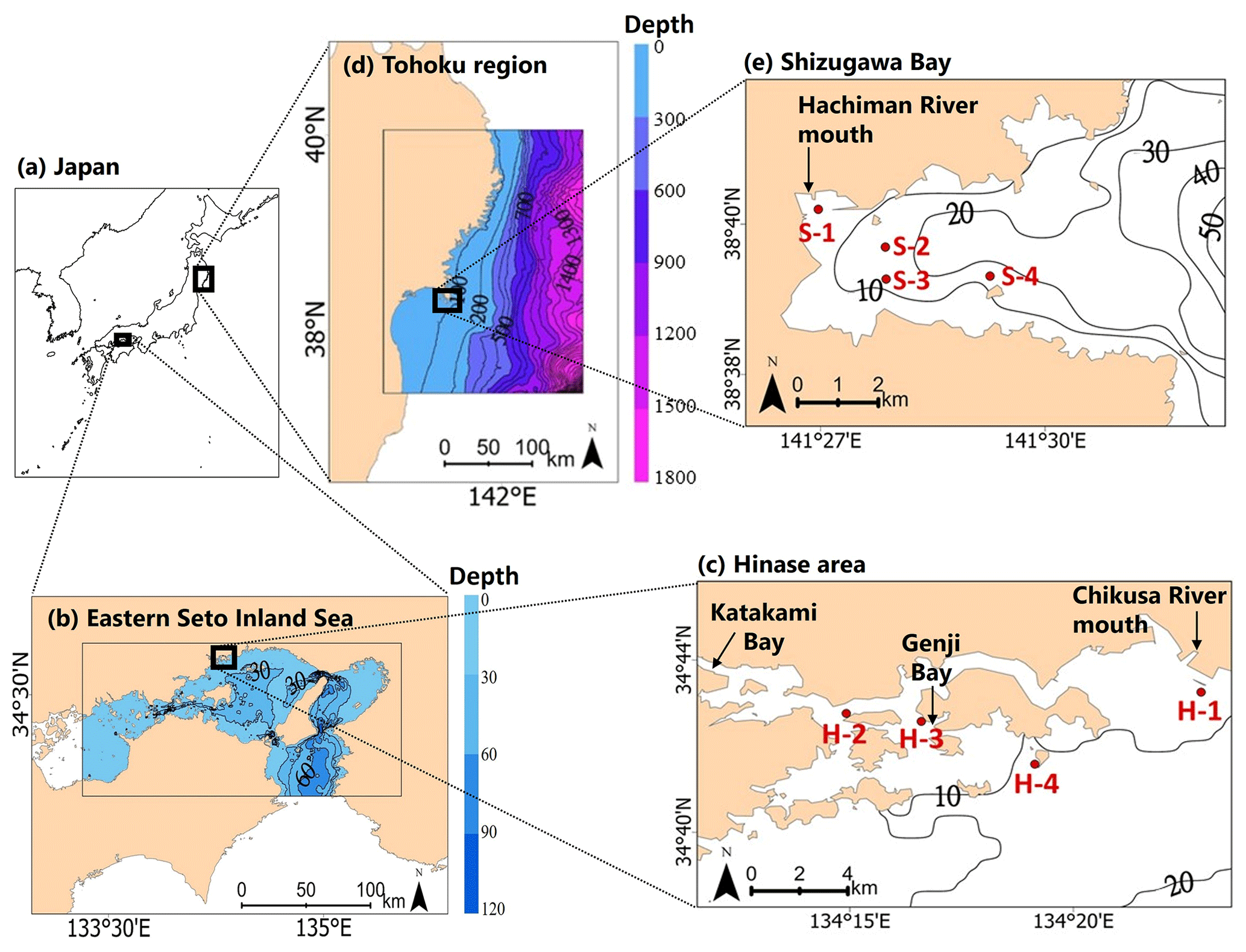
Figure 1 Map of (a) Japan, (b) the eastern Seto Inland Sea, (c) the Hinase area, (d) the Tōhoku region, and (e) Shizugawa Bay. H-1, H-2, H-3, and H-4 in (c) and S-1, S-2, S-3, and S-4 in (e) are monitoring sites in the Hinase area and Shizugawa Bay, respectively. The extent of the model grids used in each study area is also shown in (b) and (d).

Hinase is located in the Seto Inland Sea, the largest enclosed coastal sea in Japan (Association for Environmental Conservation of the Seto Inland Sea, 2022). The Seto Inland Sea is shallow, with an average depth of 38 m, and is bordered by the open sea at its southeastern, northwestern, and southwestern ends. In addition to being an enclosed sea area, excessive inflow of nutrients from the land due to human activities since the 1950s, loss of seaweed and eelgrass due to land reclamation, and frequent red tides caused by these factors have led to eutrophication of the sea area and hypoxia and anoxia in the bottom layer. Eutrophication has been overcome in many surface waters of the Seto Inland Sea through measures to control excessive inflow of nutrients from land over the last few decades, and the surface waters are even oligotrophic nowadays (e.g., Abo and Yamamoto, 2019; Yamamoto et al., 2021), but exchange of seawater with the open sea is weak, and the bottom layer is hypoxic.

Shizugawa Bay is a medium-sized bay that measures approximately 10 km east to west and 5 km north to south, with a mouth facing east (Horii et al., 1994), and has been classified as both an enclosed coastal sea (Ministry of the Environment, 2010) and an open-type bay (Komatsu et al., 2018). Since the 1990s, environmental impacts such as anoxia due to overcrowding of coho salmon and Pacific oysters have been observed (Nomura et al., 1996). Additionally, the Great East Japan earthquake of 11 March 2011 caused major damage to the social infrastructure surrounding the bay as well as the aquaculture facilities in the bay, and the subsequent tsunami affected the eelgrass and seaweed beds and tidal flats that support the fisheries.

Against this backdrop, observations of the marine environment are being conducted in both areas, with active cooperation by local fishers, within the framework of the Nippon Foundation Ocean Acidification Adaptation Project (OAAP; http://nippon.zaidan.info/jigyo/2022/0000097579/jigyo_info.html, last access: 15 November 2023), to assess acidification and to develop adaptation measures. Four monitoring sites have been set up in Hinase and Shizugawa (Fig. 1c, e). In Hinase, Site H-1 is located at the mouth of the Chikusa River, the largest river in the study site. Site H-2 is an oyster seedling site, located near the mouth of Katakami Bay. Site H-3 is an eelgrass bed, located at the mouth of Genji Bay. Site H-4 is the farthest offshore, with water depths of 10.2–12.4 m. In Shizugawa, Site S-1 is at the mouth of the Hachiman River, the largest river in the area. Site S-2 is a seaweed-farming site, and Site S-3 is a nursery for oysters. Site S-4 is the farthest offshore, and has water depths of 15.5–16.9 m.

2.2 Observation

We have measured hourly water temperature, salinity, and pH values at a depth of 1 m at each site in Hinase since 29 August 2020 and in Shizugawa since 4 September 2020, using instruments capable of continuous measurement. Dissolved oxygen (DO) has also been monitored continuously at a depth of 1–1.5 m at one site in Hinase (H-2) and one in Shizugawa (S-3) (Fig. 1c, e). A conductivity and temperature sensor (INFINITY-CTW ACTW-USB; JFE Advantech) was used to measure temperature and salinity hourly, while DO was measured hourly using a RINKO W AROW-USB (JFE Advantech). Calibration of the DO sensor was carried out by two-point (zero and span) calibration using 0 % and 100 % (saturated) oxygen waters (Fujii et al., 2021). To measure pH, glass-electrode pH sensors (SPS-14; Kimoto Electric) were used. The sensors were removed every 1–3 months for cleaning, including removal of attached organisms, data collection, battery replacement, and calibration. See Fujii et al. (2021) for details of the experimental design.

Water samples were collected when the sensors were maintained, and chlorophyll, total alkalinity (A_T), dissolved inorganic carbon (DIC), and nutrient (nitrate [NO₃], nitrite [NO₂], ammonium [NH₄], phosphate [PO₄], and silicate [Si]) concentrations were measured (Si was not assessed at Shizugawa). A_T and DIC values were obtained using a total alkalinity titration analyzer (ATT-05 by Kimoto Electronic) and a coulometer (model 3000A; Nippon ANS) (Wakita et al., 2017, 2021; Fujii et al., 2021). The values were calibrated against certified reference material provided by Andrew G. Dickson (Scripps Institution of Oceanography, University of California San Diego) and KANSO TECHNOS. The pH (total scale) values at the in situ temperatures were calculated from the carbonate dissociation constants in Lueker et al. (2000), the total boron concentration in Lee et al. (2010), the bisulfate dissociation constant in Dickson (1990), and the hydrogen fluoride dissociation constant in Perez and Fraga (1987), and temperature, salinity, A_T, and DIC were calculated using CO2SYS (Pierrot et al., 2006).

During continuous monitoring of pH, together with correction of the absolute value, it is necessary to correct for the drift of the sensor value (Yamaka, 2019; Fujii et al., 2021). In this study, the pH value of a pH sensor at time t (pH(t)) was obtained using the following equation (Hamanoue, 2022):

$$\begin{array}{}\text{(3)}& \begin{array}{rl}\mathrm{pH}\left(t\right)& ={\mathrm{pH}}_{\mathrm{m}}\left(t\right)+[\left({\mathrm{pH}}_{\mathrm{sample}}\left(t_{\mathrm{i}}\right)-{\mathrm{pH}}_{\mathrm{m}}\left(t_{\mathrm{i}}\right)\right)\\ & +\mathit{\left\{}{\mathrm{pH}}_{\mathrm{sample}}\right(t_{\mathrm{e}})-{\mathrm{pH}}_{\mathrm{m}}(\mathrm{d}{t}_{\mathrm{e}})\\ & -\left({\mathrm{pH}}_{\mathrm{sample}}\left(t_i\right)-{\mathrm{pH}}_{\mathrm{m}}\left(t_{\mathrm{i}}\right)\right)\mathit{\left\}}\right]\times {\displaystyle \frac{t-t_{\mathrm{i}}}{t_{\mathrm{e}}-t_{\mathrm{i}}}},\end{array}\end{array}$$

where pH_m(t) represents the measured value of pH at time t; pH_sample(t_e) and pH_sample(t_i) are the pH values at the end time (t_e) and start time (t_i) of each deployment, respectively, obtained by the seawater sample and sensor; and pH_m(t_i) is the pH value measured by the sensor at time t_i; pH_m(dt_e) is the minimal or average pH value measured by the sensor for 24 h prior to t_e. pH increases during the day due to photosynthesis and decreases during the night due to respiration of organisms. If algae or other organisms adhere to the glass-electrode portion of the sensor, the effect of photosynthesis during the day is amplified, and the pH value is overestimated. To minimize calibration uncertainty due to this effect, the lowest daily value was used for pH_m(dt_e) if an effect of photosynthesis was observed in the previous 24 h, and the average value was used if not.

Ω_arag can be calculated using two of the following values in addition to water temperature and salinity – pH, A_T, DIC, and CO₂ concentration in seawater. Of these, the A_T and DIC values were calculated by the above when seawater was sampled, but such sampling was conducted only once or twice per month. Therefore, because the A_T of seawater is highly correlated with salinity (e.g., Yamamoto-Kawai et al., 2015), a regression equation was calculated from the salinity and A_T values of the seawater samples (Fig. 2a, b). Hourly A_T values were estimated from hourly salinity data obtained from continuous observations. Hourly values of Ω_arag were calculated using CO2SYS (Lewis et al., 1998), together with water temperature and pH values obtained from continuous observations. The maximum error for this process of determining alkalinity from salinity is about 30 µmol kg⁻¹ and 0.06 for alkalinity and Ω_arag, respectively.

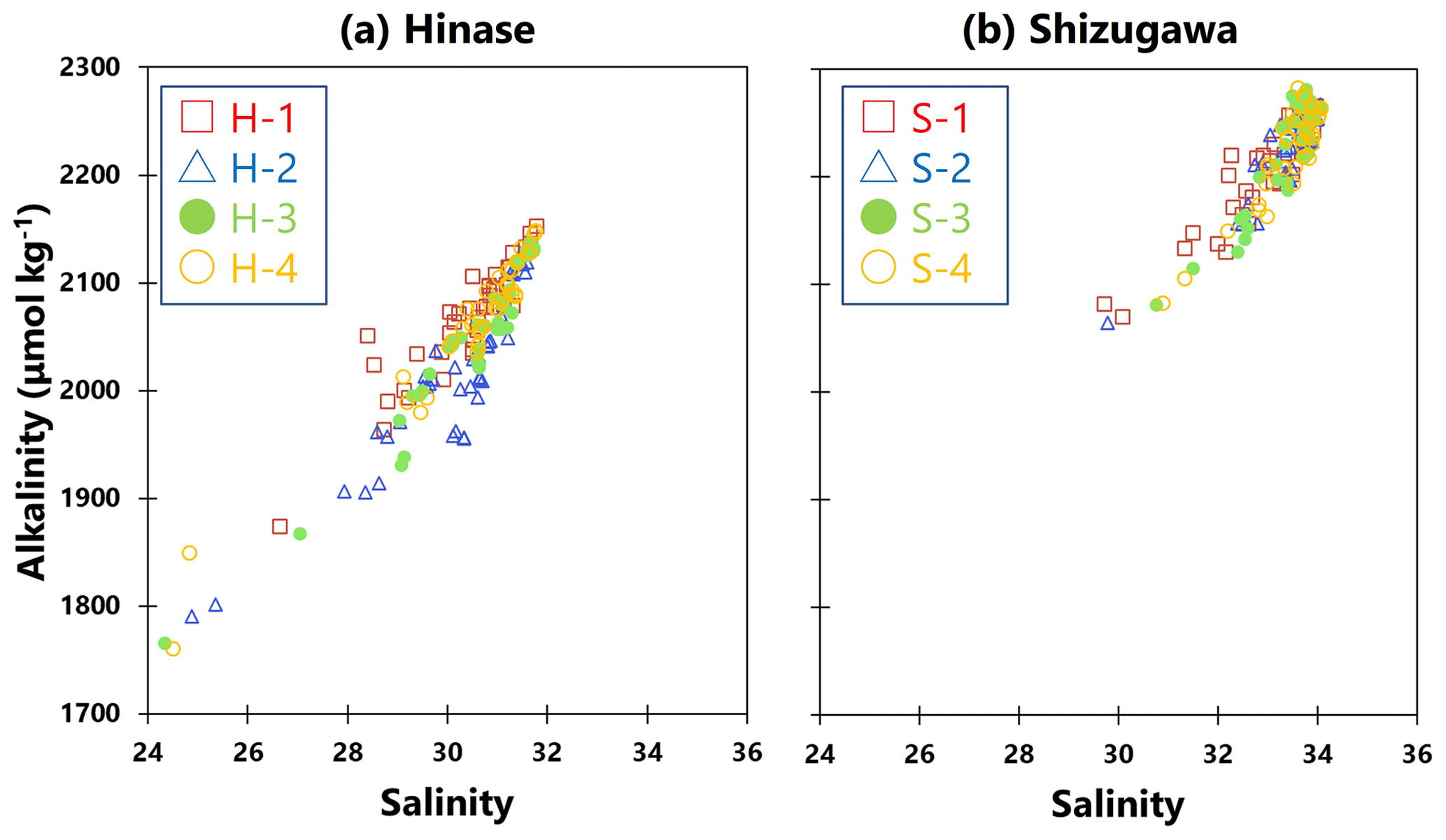
Figure 2 Observed total alkalinity (A_T) vs. salinity in (a) Hinase (H-1 (open red square), H-2 (open blue triangle), H-3 (solid green circle), and H-4 (open orange circle)) and (b) Shizugawa (S-1 (open red square), S-2 (open blue triangle), S-3 (solid green circle), and S-4 (open orange circle)). Correlation coefficients: H-1, R²=0.86; H-2, R²=0.85; H-3, R²=0.92; H-4, R²=0.94; S-1, R²=0.88; S-2, R²=0.85; S-3, R²=0.90; and S-4, R²=0.90.

To examine the effects of precipitation and freshwater inflow from rivers on the spatiotemporal changes in acidification indices, precipitation data from the sites nearest to Hinase (Mushiage, Oku (town), Setouchi, Okayama Prefecture) and Shizugawa (Shizugawa, Minamisanriku (town), Miyagi Prefecture) (Japan Meteorological Agency website; https://www.data.jma.go.jp/obd/stats/etrn/index.php, last access: 14 November 2023) were obtained. The precipitation data were compared directly with the spatiotemporal changes in salinity, pH, and Ω_arag to verify whether variations were due to precipitation or inflow from rivers.

2.3 Microscopic examination of oyster larvae

Like other calcifying organisms, Pacific oysters (C. gigas) are particularly vulnerable to acidification at the larval stage. By incubating Pacific oysters in a high-CO₂ tank, Kurihara et al. (2007) revealed that acidified water inhibited the growth of D-shaped veliger larvae. Thus, microscopic examination of D-shaped veliger larvae enables assessment of the impact of acidification on Pacific oysters.

Microscopic examination of D-shaped veliger larvae collected using 50–100 µm mesh plankton nets was carried out in Hinase and Shizugawa during the spawning season. In Hinase, the examination was performed at the Hinasecho Fisheries Cooperative Association from 4 July to 31 August 2020 (n=370) and from 21 June to 1 October 2020 (n=244), and at the Okucho Fisheries Cooperative Association from 11 July to 9 September 2020 (n=292) and from 2 July to 30 August 2021 (n=156). In Shizugawa, microscopy examination was performed at the Kesennuma Miyagi Prefectural Fisheries Experimental Station from 27 July to 2 September 2020 (n=60) and 26 July to 6 September (n=70).

2.4 Modeling

To reproduce the coastal environment in Hinase and Shizugawa and to project future conditions, the Regional Ocean Modeling System (ROMS) was used. Of the versions of ROMS, we chose CROCO (version 1.1; Jullien et al., 2019), which can perform high-resolution simulations and account for various interactions, including atmosphere, tides, and bathymetry. In addition, CROCO enables coupling of ROMS with the Pelagic Interaction Scheme for Carbon and Ecosystem Studies (PISCES; Aumont et al., 2003; Aumont, 2005), a marine ecosystem model, enabling calculation of biogeochemical as well as physical processes (Hamanoue, 2022; Bernardo et al., 2023). The model is therefore suitable for simulating complex coastal marine environments.

The prognostic variables for the physical processes of the model were water temperature and salinity, and those for the biogeochemical processes were DO, A_T, DIC, and nutrients (NO₃, PO₄, Si). pH and Ω_arag were calculated from the values of water temperature, salinity, A_T, and DIC obtained by the model using CO2SYS. The unavoidable biases in model results of prognostic variables relative to observed values were corrected using the procedure adapted by Yara et al. (2011) and Fujii et al. (2021).

The model domain was set to 133^∘38^′06^′′ to 135^∘47^′67^′′ E and 33^∘93^′24^′′ to 34^∘79^′81^′′ N in Hinase (Fig. 1b) and 140^∘86^′10^′′ to 142^∘86^′20^′′ E and 37^∘59^′47^′′ to 39^∘76^′47^′′ N in Shizugawa (Fig. 1d). The horizontal resolution of the models was approximately 2 km. The vertical coordinate system was the σ coordinate system, and the number of layers was 32. Bathymetry was derived using the 15 arcsec (∼ 500 m near the Equator) General Bathymetric Chart of the Oceans (2021) dataset (GEBCO website; Table 1). Model output data were at 6 h intervals (Bernardo et al., 2023). Representative simulations were carried out for present and future (2090s) conditions. Each simulation was carried out for a 1-year and 3-month period from May to July (2000 to 2001 for the present and 2099 to 2100 for the future), and the daily mean results at 1 m depth were used for analysis and comparison with the observed results.

Table 1 Boundary conditions for the coupled physical–biogeochemical model used in this study. For boundary conditions of dissolved oxygen (DO) and nutrients, the present replicate values were given for the 2090s.

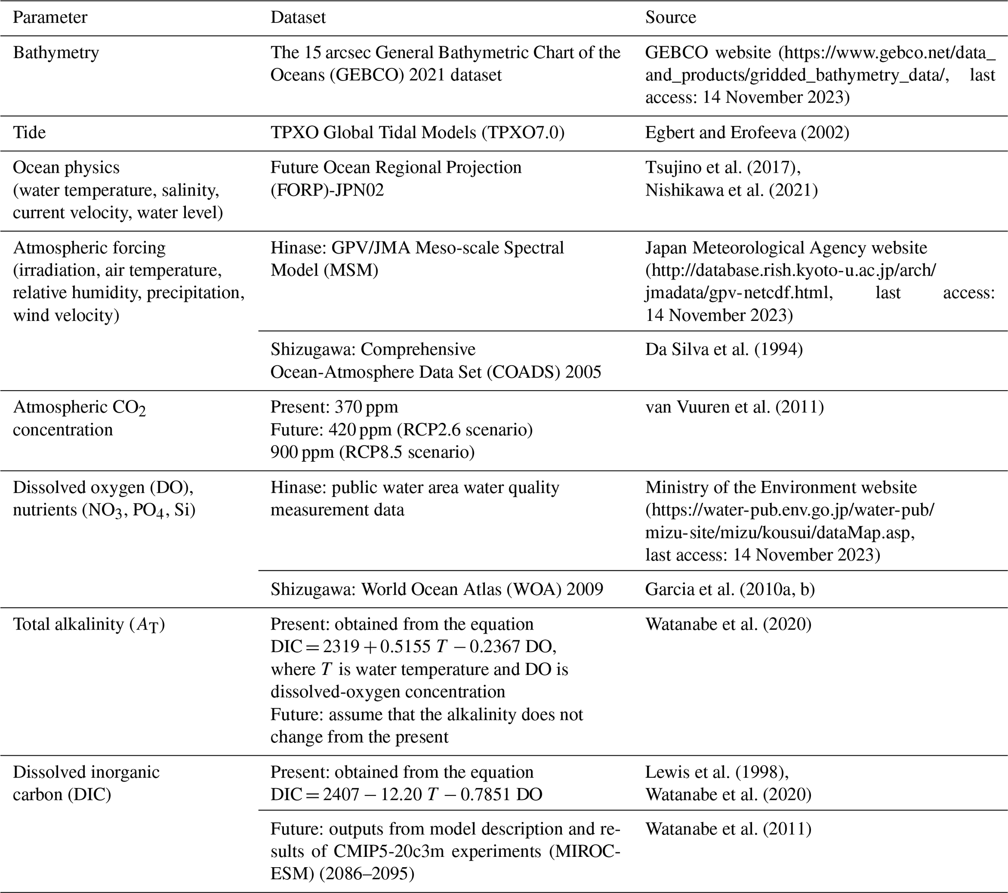
The boundary conditions for water temperature, salinity, current velocity, and the water level were taken from the Future Ocean Regional Projection (FORP)-JPN02 version-2 dataset (Nishikawa et al., 2021), which has a horizontal resolution of 2 km, the highest resolution for Japan to date. For the future greenhouse gas emissions scenarios, we used the MRI-CGCM3 climate prediction model outputs developed at the Meteorological Research Institute (Tsujino et al., 2017) under the Representative Concentration Pathway (RCP) 2.6 and 8.5 scenarios (van Vuuren et al., 2011) of the Coupled Model Intercomparison Project Phase 5 (CMIP5; Taylor et al., 2012). Table 1 lists the boundary conditions used in this study.

2.5 Thresholds for evaluating the impacts on Pacific oysters (C. gigas)

Pacific oysters (C. gigas) reach sexual maturity when the accumulated water temperature reaches 600 ^∘C based on a water temperature of 10 ^∘C, and at water temperatures of 20 ^∘C or higher they spawn once and then mature and spawn again (Oizumi et al., 1971). Therefore, there is a concern that a rise in water temperatures in the future may cause earlier or longer spawning and maturation times. The earlier spawning and maturation times may result in a mismatch with existing oyster-farming approaches. The prolonged spawning period may shorten the oyster shipping period and lower the oysters' quality (Akashige and Fushimi, 1992), potentially damaging the oyster-processing industry. In this study, based on Oizumi et al. (1971), spawning was assumed to start when the accumulated water temperature reaches 600 (^∘C day) based on a water temperature of 10 ^∘C and to end when the water temperature drops below 20 ^∘C. There are no previous studies that set the threshold for the impact of ocean acidification on Pacific oysters on Japan coasts. Therefore, to evaluate the impact of ocean acidification on Pacific oysters, we referred to a threshold of Ω_arag=1.5 (Waldbusser et al., 2015), which was obtained from rearing experiments of Pacific oyster larvae in Oregon, USA, and hence, the species and reaction to local environment may be different from those on Japan coasts. Below that threshold, the development of Pacific oyster larvae is likely to be affected, with slower growth and higher mortality.

To evaluate the impact of deoxygenation on Pacific oysters, we referred to a threshold DO concentration of 203 µmol kg⁻¹ as a lower limit of the optimal DO range for Pacific oyster growth (Hochachka, 1980; Fisheries Agency, 2013).

3 Results

3.1 Observation results

Water temperatures showed significant seasonal variations at both sites (Fig. 3a–h). In Hinase, the highest water temperature during the observation period was 32.3 ^∘C at H-2 on 8 August 2021 (Fig. 3b). The highest water temperatures at the other sites in Hinase were observed in August 2020, with a maximum temperature difference of 1.2 ^∘C between sites. The lowest water temperatures were observed in the middle of January 2021: 6.2 ^∘C at H-1, 3.9 ^∘C at H-2, 5.6 ^∘C at H-3, and 7.3 ^∘C at H-4 (Fig. 3a–d). In Shizugawa, the highest water temperature during the observation period was 28.7 ^∘C at S-2 on 6 August 2021 (Fig. 3f), and the highest water temperatures at the other sites were observed on 8 September 2020 or 6 August 2021 (Fig. 3e, g, h). The lowest water temperature of 6.5 ^∘C was observed at S-1 on 9 February 2021 (Fig. 3e). The difference between sites was about 0.8 and 0.7 ^∘C for the maximum and minimum water temperatures, respectively.

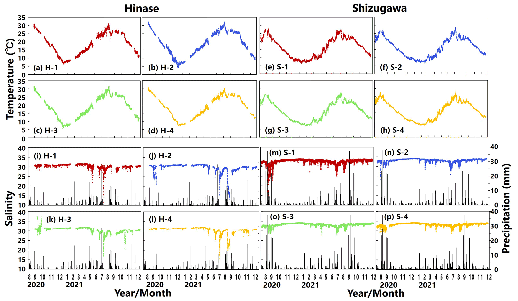
Figure 3 Observed temperature (^∘C) (top; a–h) and salinity (bottom; i–p) values in Hinase (H-1, H-2, H-3, and H-4) and Shizugawa (S-1, S-2, S-3, and S-4) from August 2020 to December 2021. Black bars in (i)–(p) indicate hourly precipitation (mm) at the nearest Automated Meteorological Data Acquisition System (AMeDAS) station – Mushiage (Hinase) and Shizugawa (Shizugawa) (Japan Meteorological Agency website; https://www.data.jma.go.jp/obd/stats/etrn/index.php, last access: 14 November 2023).

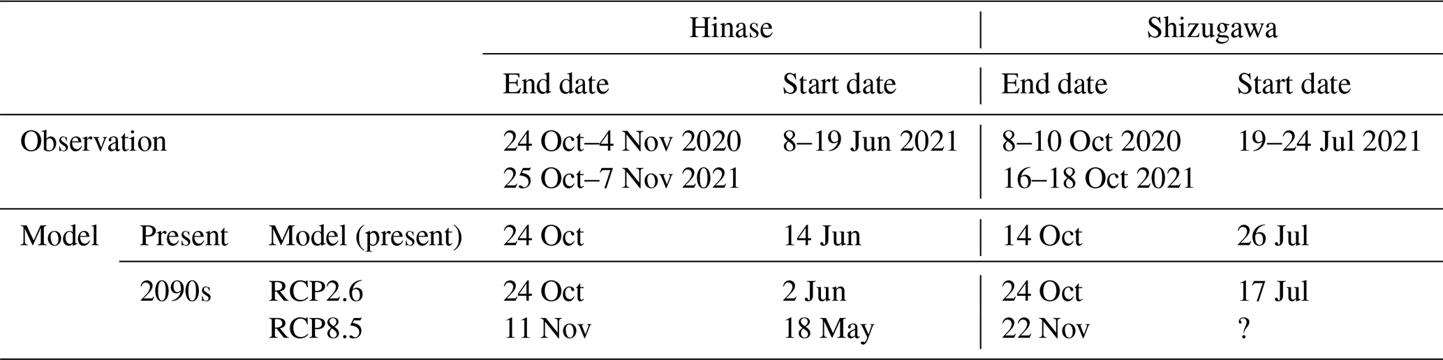
As mentioned in Sect. 2.5, spawning periods of Pacific oysters are estimated from the water temperature thresholds based on Oizumi et al. (1971) (Table 2). In Hinase, Pacific oysters were estimated to have stopped spawning between 24 October and 4 November 2020 and between 25 October and 7 November 2021 and to have begun spawning between 8 and 19 June in 2021, judging from the water temperature thresholds based on Oizumi et al. (1971). In Shizugawa, spawning was estimated to have ended between 8 and 10 October 2020 and between 16 and 18 October 2021 and to have begun between 19 and 24 July 2021.

Table 2 End and start dates of Pacific oyster (C. gigas) spawning in Hinase and Shizugawa, estimated from observed present and modeled present and future water temperatures and based on Oizumi et al. (1971).

Salinity usually varied between 30.5 and 31.5 at sites in Hinase and between 32 and 34 in Shizugawa (Fig. 3i–p). In the Hinase area, the minimum salinity at H-1, H-2, H-3, and H-4 during the monitoring period was 11.4, 13.3, 16.5, and 15.3 and appeared on 9 July, 23 August, 10 July, and 10 July 2021, respectively (Fig. 3i–l). The lowest salinity at H-1, H-3, and H-4 appeared on 9–10 July, and the second-lowest salinity at H-2 during the monitoring period (15.4) similarly appeared on 11 July 2021 (Fig. 3j); the heaviest rainfall during the monitoring period (hourly precipitation of 28.5 mm) around the sites occurred at 04:00 LT (Japan standard time) on 8 July 2021, i.e., 1 or 2 d before the lowest salinity appeared at the sites. The lowest salinity at H-2 appeared on 23 August 2021, after intermittent rainfall which lasted for several days from 12 August 2021. In the Shizugawa Bay, the minimum salinity at S-1, S-2, S-3, and S-4 during the monitoring period was 15.2, 23.5, 27.9, and 28.8 and appeared on 5 September 2020, 23 August 2020, 2 May 2021, and 11 July 2021, respectively (Fig. 3m–p). The extremely low salinity observed at S-1 (located at the mouth of the Hachiman River) at 17:00 LT on 5 September 2020 (Fig. 3m) seemed to be caused by the heaviest rainfall during the monitoring period, which was recorded on that day (hourly precipitation of 37.5 mm at 08:00 LT; 9 h earlier than the appearance of the lowest salinity at S-1); presumably the increased freshwater discharge from the Hachiman River followed the heavy rainfall. Although the relation between the salinity and rainfall during the entire period of monitoring was not statistically significant at any of the sites in Hinase and Shizugawa, extremely low salinity seems to be related to direct freshwater input from the rainfall and subsequently increased freshwater discharge from nearby rivers. Rainfall does not always result in a significant decrease in salinity, but when there is a significant decrease in salinity, it always tends to be after rainfall events.

The observed nutrient concentrations differed among sites and had large seasonal and interannual fluctuations, being relatively high in late summer and autumn and low in the other periods (not shown). The observed range of NO₃ concentration was 0.01–8.18 µmol kg⁻¹ in Hinase and 0.00–4.75 µmol kg⁻¹ in Shizugawa. That of PO₄ concentration was 0.03–1.29 µmol kg⁻¹ in Hinase and 0.01–0.74 µmol kg⁻¹ in Shizugawa. It is difficult to assess if the waters are oligotrophic or not by certain thresholds of nutrient concentrations. On the other hand, if we refer to the half-saturation constant of each nutrient concentration given in the model (e.g., 0.26–1.3 µmol kg⁻¹ for NO₃ and 0.0008–0.004 µmol kg⁻¹ for PO₄ in Aumont, 2005), NO₃ and PO₄ are considered to be depleted, which is regarded as an oligotrophic condition in some seasons in the surface water in both sites.

DO concentrations showed significant seasonal variation, generally being high in winter and low in summer at all sites in Hinase (Fig. 4a) and Shizugawa (Fig. 4b). Although the DO concentrations were above the lower limit of the optimal DO range for Pacific oyster growth (203 µmol kg⁻¹; Hochachka, 1980; Fisheries Agency, 2013) in Shizugawa, they were often below the optimal range in summer and autumn in Hinase.

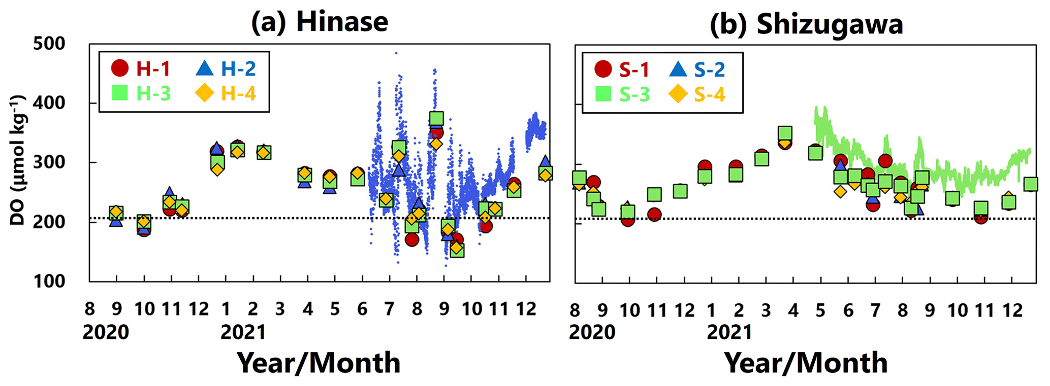
Figure 4 Time series of dissolved-oxygen (DO; µmol kg⁻¹) values in (a) Hinase and (b) Shizugawa. Measurements were carried out when water-bottle samples were collected, and solid red circles (H-1 and S-1), solid blue triangles (H-2 and S-2), solid green squares (H-3 and S-3), and solid yellow diamonds (H-4 and S-4) are measured values. Continuous monitoring using sensors was performed after 10 June 2021 at H-2 (in blue dots) and after 27 April 2021 at S-3 (in green dots). The monitored values are shown as dots (blue at H-2 and green at S-3). The lower threshold of the optimal DO range for the growth of Pacific oyster (C. gigas) (203 µmol kg⁻¹; Hochachka, 1980; Fisheries Agency, 2013) is denoted by a dotted line.

A_T values estimated from continuous salinity observations using the abovementioned regression equation (Fig. 2) matched those determined by water-sample analysis at each site (Fig. 5a–h). The estimates implied a significant decrease in A_T values, associated with a localized decrease in salinity as a result of rainfall and subsequent enhanced riverine discharge, that could not be captured by once- or twice-monthly water-sample analysis.

DIC values determined by water-sample analysis showed clear seasonal variation, being generally high in winter and low in summer (Fig. 5i–p), likely a result of the higher solubility of atmospheric CO₂ at low temperatures and more vigorous primary production, respectively. The DIC estimated from water temperature, salinity, and pH (and A_T via salinity) showed similar fluctuations to the corresponding A_T. In contrast, the estimated DIC showed abrupt changes at all sites that were not captured by water-sample analysis. Abrupt drawdowns of estimated DIC were sometimes found, and a significant decrease occurred at all four sites in Hinase on 13 July 2021 (Fig. 5i–l), after a major rainfall event.

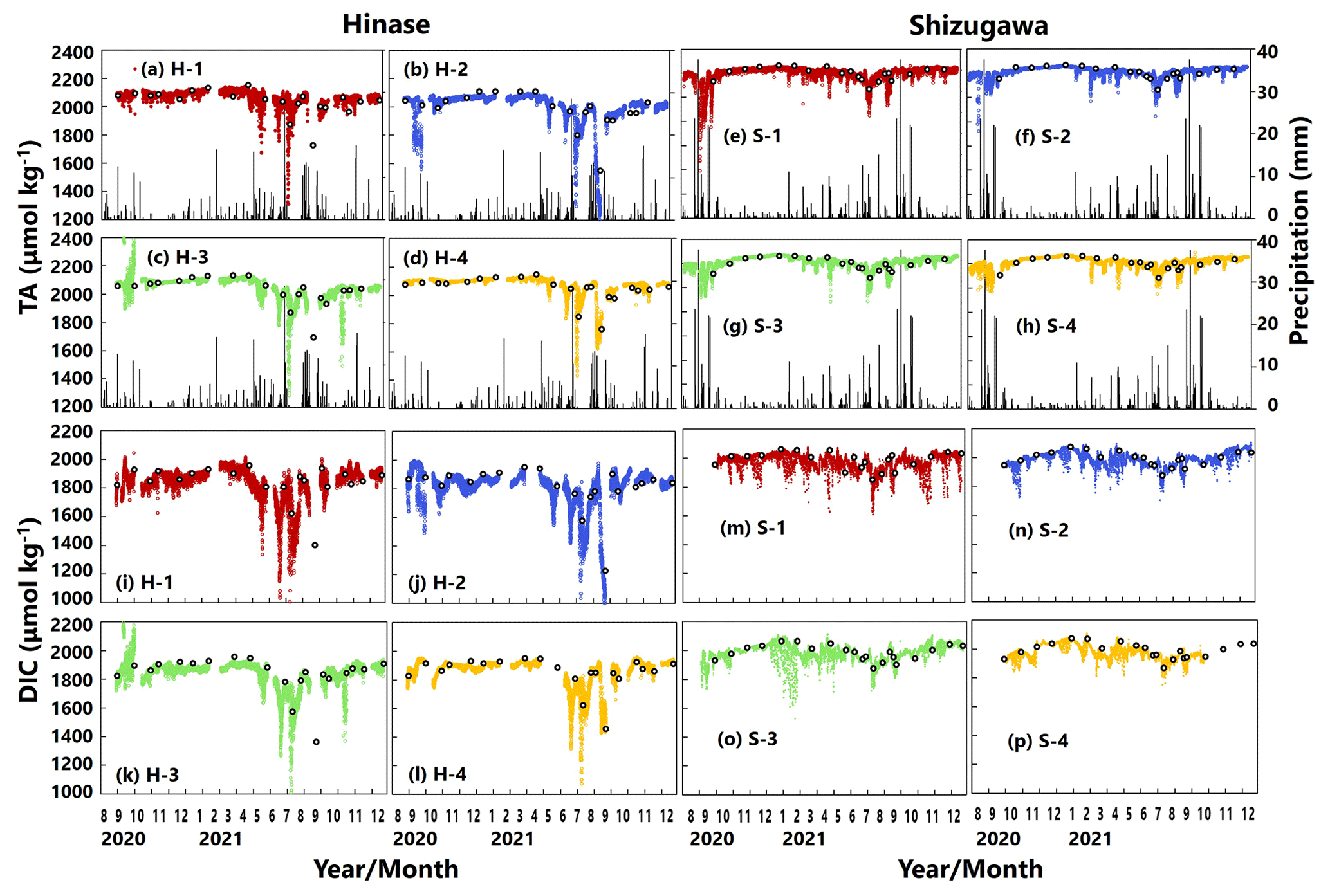
Figure 5 Total alkalinity (A_T (µmol kg⁻¹); a–h) and dissolved inorganic carbon (DIC (µmol kg⁻¹); i–p) values based on water-sample analysis (open circles) and estimated from continuously observed salinity (colored dots) in Hinase (H-1 to H-4) and Shizugawa (S-1 to S-4) from August 2020 to December 2021. Black bars in (a)–(h) indicate hourly precipitation (mm) at the nearest AMeDAS stations (Japan Meteorological Agency website; https://www.data.jma.go.jp/obd/stats/etrn/index.php, last access: 14 November 2023).

pH values varied widely during the observation period at all sites in Hinase and Shizugawa, with a marked decrease after rainfall (Fig. 6a–h). The extent of the post-rainfall decline in pH differed among the sites. In Hinase, the lowest pH was in September 2021 (Fig. 6a–d), and pH values were lower at H-1, H-2, and H-3 than at H-4, which was the farthest offshore. After rainfall on September 2021, the lowest pH values at H-1 and H-2 were 0.2 units lower than those at the other two sites. In Shizugawa, the lowest pH value of 7.8 occurred in July and August 2021, at S-1 and S-3 (in the estuary and offshore, respectively) (Fig. 6e, g).

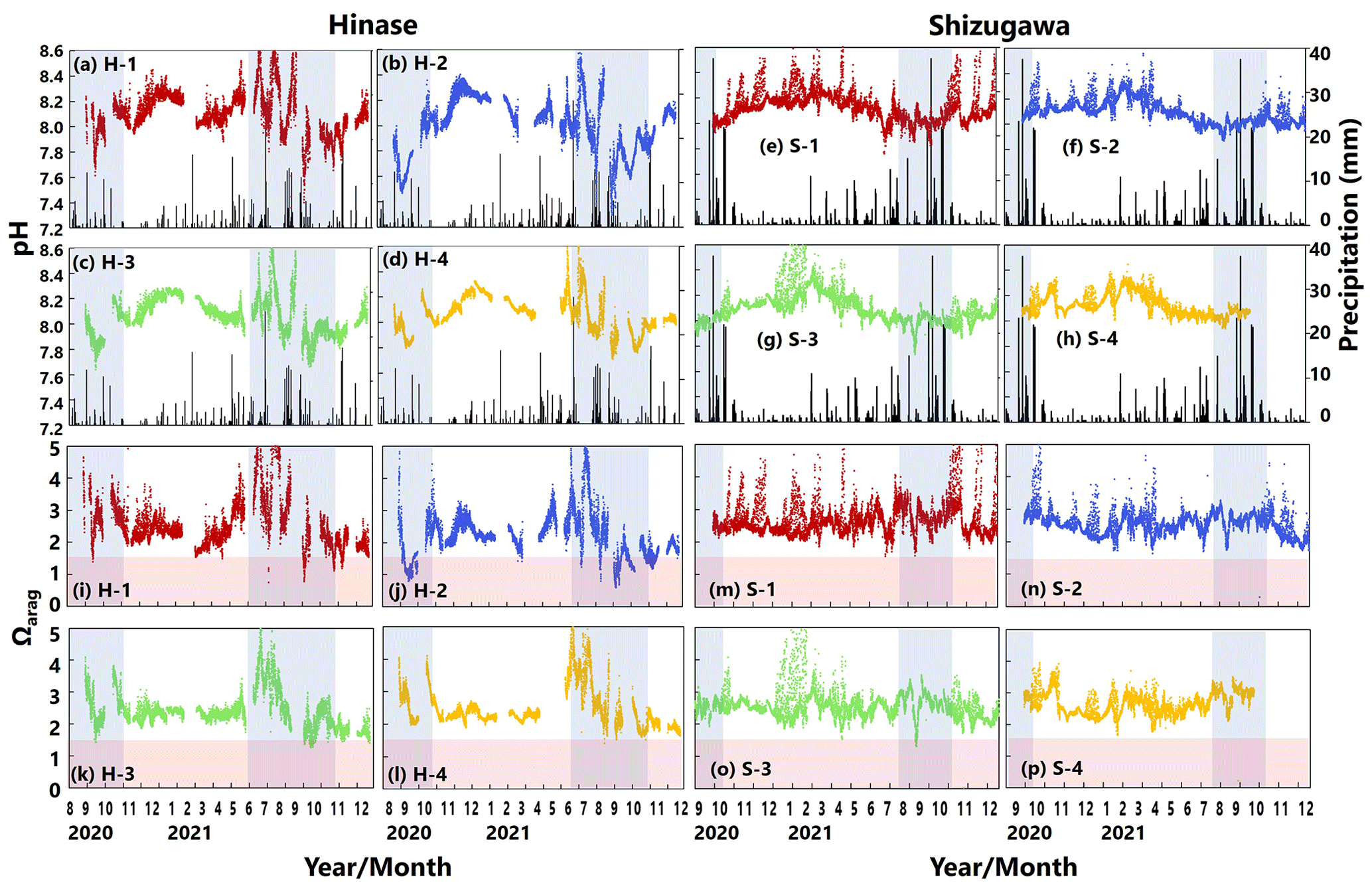
Figure 6 Observed pH (a–h) and aragonite saturation state (Ω_arag) (i–p) in (a) Hinase (H-1, H-2, H-3, and H-4) and (b) Shizugawa (S-1, S-2, S-3, and S-4) from August or September 2020 to December 2021. Red domains denote the critical level of acidification for Pacific oyster larvae in Waldbusser et al. (2015) (Ω_arag<1.5). Blue domains denote the spawning season of Pacific oyster estimated from Oizumi et al. (1971). Black bars in (a)–(h) indicate hourly precipitation (mm) at the nearest AMeDAS stations (Japan Meteorological Agency website; https://www.data.jma.go.jp/obd/stats/etrn/index.php).

Ω_arag varied significantly during the observation period at all sites in Hinase and Shizugawa (Fig. 6i–p). The temporal variability varied from site to site, with greater decreases at sites closer to the coast. Ω_arag values < 1.5 were often detected in Hinase, especially at H-1 and H-2 (Fig. 6i, j), which were close to the river. Furthermore, during the spawning season of Pacific oysters from June to October or November (Oizumi et al., 1971), values fell below that threshold locally; the lowest Ω_arag of 0.8 was observed at H-2, which is used as a nursery for oysters, and values remained below the threshold for 2 weeks (Fig. 6j). In Shizugawa, the Ω_arag value was below the threshold only in August 2021 at S-3 for 4 h (Fig. 6o, p), coinciding with the spawning season of Pacific oysters. However, no morphological abnormalities were observed in the larvae from Hinase and Shizugawa (Fig. 7), and therefore, we did not find any anecdotal evidence of impacts of ocean acidification on Pacific oyster larvae in this study.

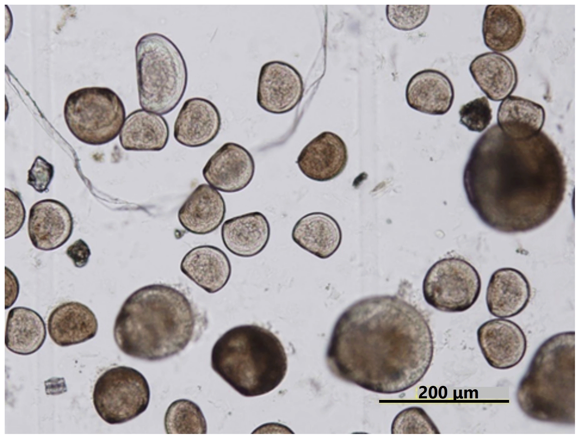
Figure 7 Micrograph of Pacific oyster larvae in Hinase. No morphological abnormalities were observed.

3.2 Modeling results

The model successfully reproduced the spatiotemporal variations in each parameter in Hinase and Shizugawa (Figs. 8 and 9), such as significant seasonal fluctuation in water temperature (Figs. 8a–d, 9a–d). The modeled salinity was relatively uniform in space and season. However, the salinity was lower in coastal regions in Hinase, especially near rivers in summer where and when freshwater discharge from rivers is dominant (Fig. 8e–h). The spatiotemporal variability was lower in Shizugawa, although the seawater flowing into the bay is likely influenced by freshwater discharged from the Kitakami River, the fifth-longest river in Japan (Fig. 9e–h). The modeled DO is in direct contrast with water temperature, higher in winter and lower in summer (Figs. 8i–l and 9i–l), primarily caused by higher and lower solubility of oxygen in cooler and warmer water, respectively.

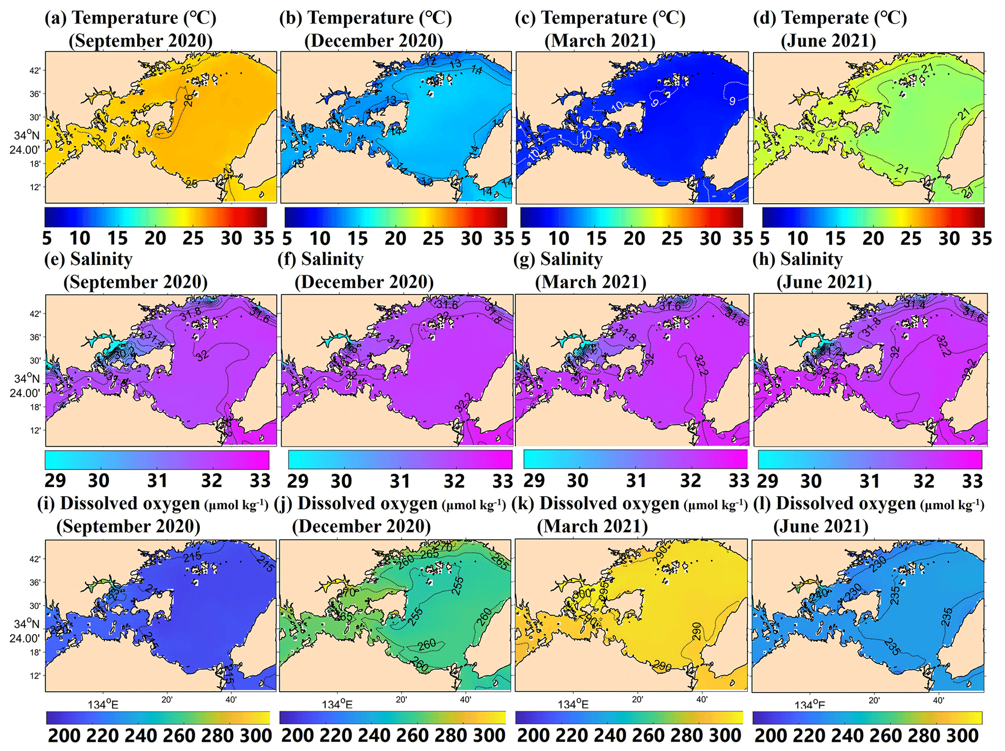
Figure 8 Horizontal distribution of modeled monthly-mean surface temperature (^∘C; a–d), salinity (e–h), and DO (µmol kg⁻¹; i–l) in September, December, March, and June in the model domain of the Hinase area.

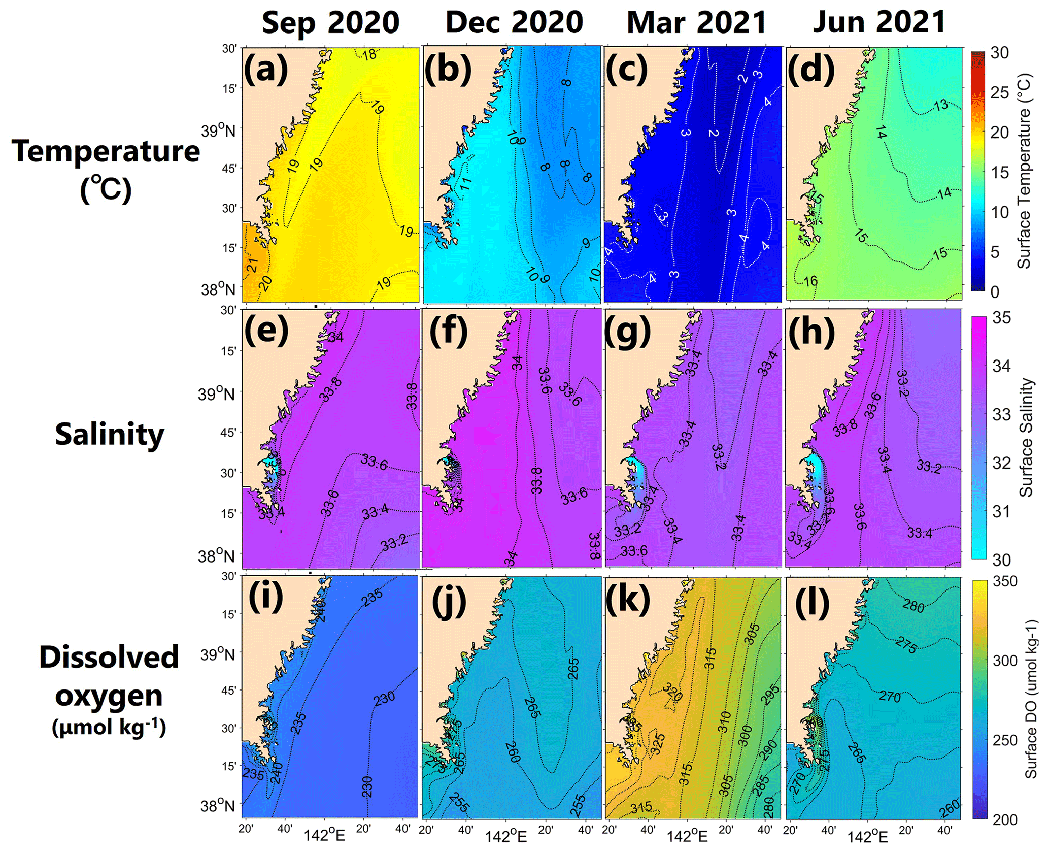
Figure 9 Horizontal distribution of modeled monthly-mean surface temperature (^∘C; a–d), salinity (e–h), and DO (µmol kg⁻¹; i–l) in September, December, March, and June in the model domain of Shizugawa Bay.

The modeled temperature reproduced the observed seasonal fluctuations in Hinase (Fig. 10a–d) and Shizugawa (Fig. 10e–h). However, the modeled seasonal fluctuation in temperature was around 1 month behind observations in Shizugawa. The model–observations mismatch may be a result of the internal variability in the climate model (Yara et al., 2011), especially for the Pacific Ocean, which provided the boundary conditions used in this study. Nonetheless, based on Oizumi et al. (1971), the current start and end dates of the Pacific oyster spawning period were calculated to be on 14 June in Hinase and 26 July in Shizugawa and on 24 October in Hinase and 14 October in Shizugawa, respectively. These are consistent with the observation-based estimated start dates (8–19 June in Hinase and 19–24 July in Shizugawa) and end dates (24 October–7 November in Hinase and 8–18 October in Shizugawa), respectively (Table 2). The observed sudden decrease in the salinity was reproduced but was underestimated by the model (Fig. 10i–p).

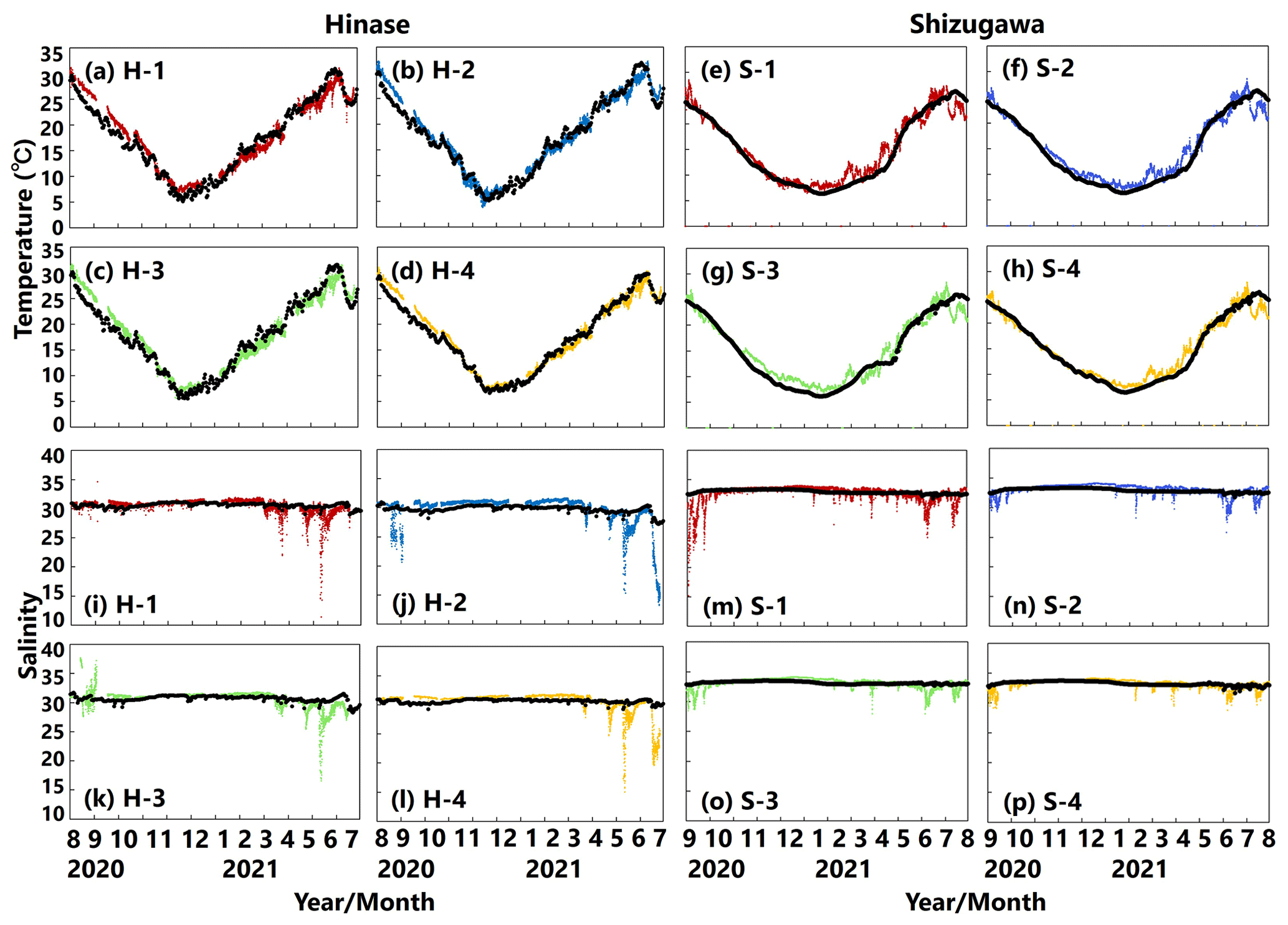
Figure 10 Observed (colored dots) and modeled (black lines) water temperature (a–h) and salinity (i–p) at 1 m depth in Hinase (August 2020 to July 2021) and Shizugawa (September 2020 to August 2021).

The modeled DO, A_T, and DIC values reproduced the observed seasonal fluctuations in Hinase and Shizugawa (Figs. 11a–b and 12a–p). However, the model did not reproduce the short-term fluctuations in biogeochemical parameters. This was mainly because the temporal resolution of the model output is 6 h, insufficient to resolve significant short-term fluctuations in biogeochemical processes predominantly caused by biological activities, i.e., photosynthesis by phytoplankton, eelgrass, and seaweeds during the day and respiration of marine organisms at night. Although the spatial resolution of the model (2 km) is relatively high for downscaling climate model outputs, it is insufficient to reproduce spatial differences in biogeochemical-parameter values among the four sites in Hinase and Shizugawa. Also, the model–observations mismatch for A_T and DIC values, especially the failure to reproduce sudden decreases, likely resulted from insufficient input of freshwater from rainfall and riverine water into the model.

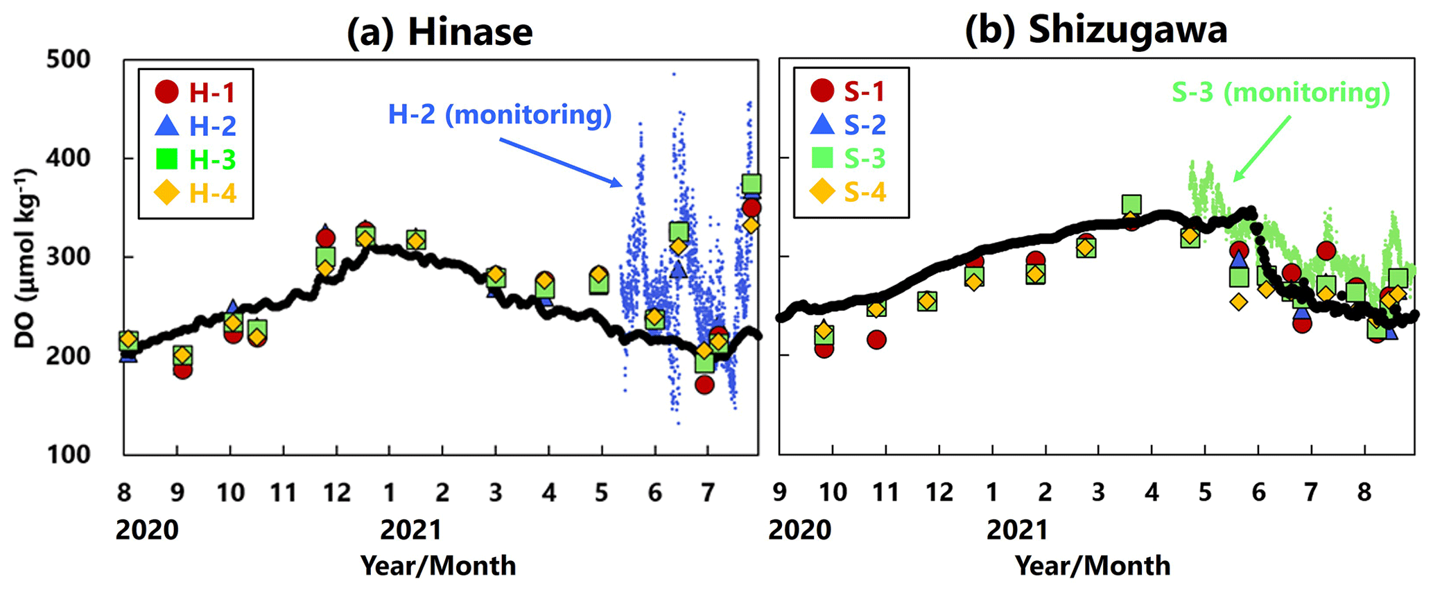
Figure 11 Observed (red circles (H-1 and S-1), blue triangles (H-2 and S-2), green squares (H-3 and S-3), and orange diamonds (H-4 and S-4)) and modeled (black lines) DO concentration (µmol kg⁻¹) at 1 m depth in (a) Hinase (August 2020 to July 2021) and (b) Shizugawa (September 2020 to August 2021). The monitored values are shown as dots (blue at H-2 and green at S-3).

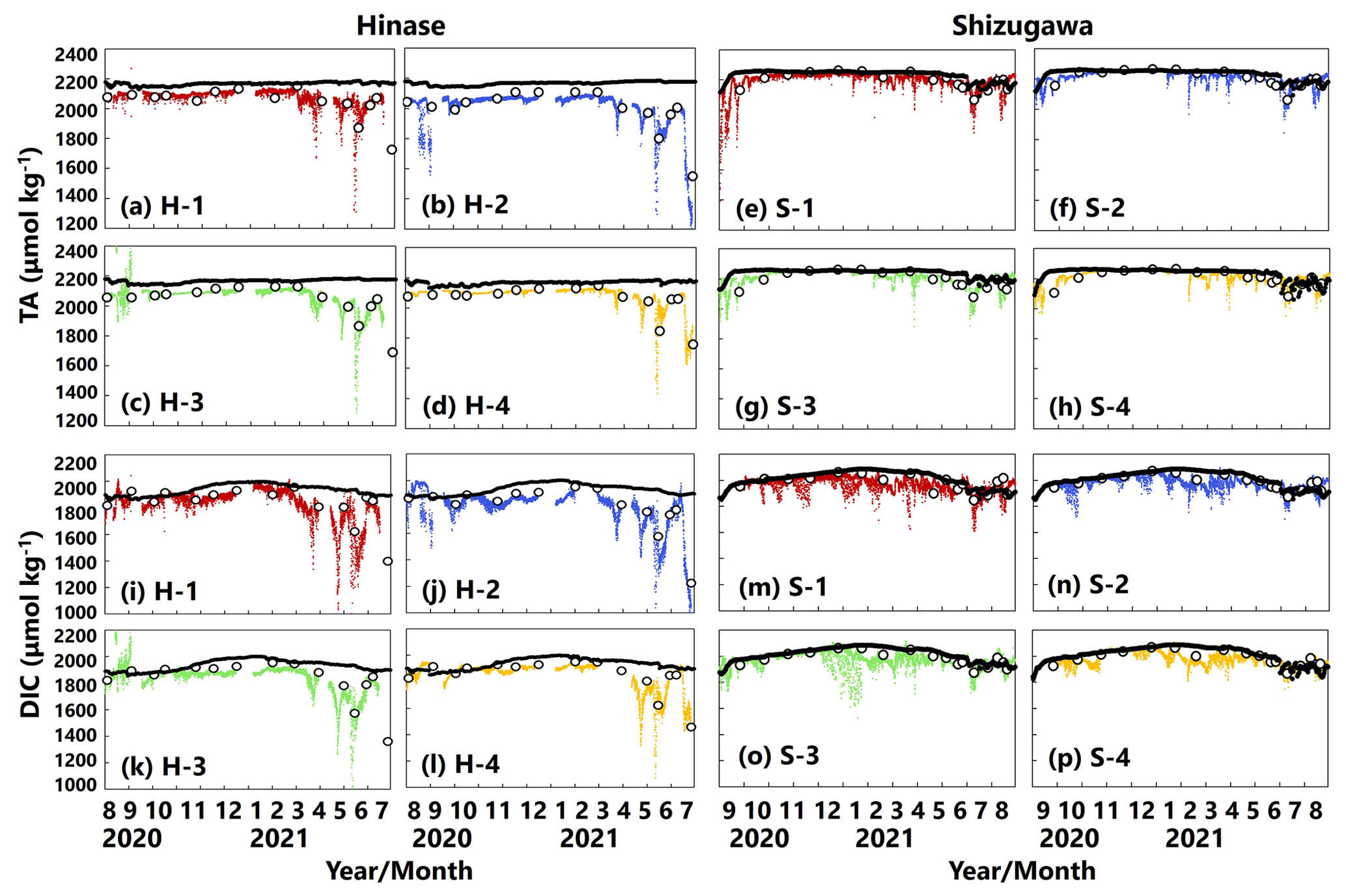
Figure 12 Observed (colored dots) and modeled (black lines) A_T (a–h; µmol kg⁻¹) and DIC (i–p; µmol kg⁻¹) concentration at 1 m depth in Hinase (August 2020 to July 2021) and Shizugawa (September 2020 to August 2021).

The modeled pH and Ω_arag values reproduced those observed (Fig. 13a–p). However, similarly to for the other biogeochemical parameters, the model had difficulty in simulating short-term fluctuations. Because the model's pH and Ω_arag values are calculated from modeled temperature, salinity, A_T, and DIC values, uncertainties in the latter could magnify or cancel out those in the former. The estimated number of days on which Ω_arag values are below the threshold of acidification for Pacific oyster larvae (1.5) at present by the model results is 0 d in both Hinase and Shizugawa. The number of days is modified to 3 d in Hinase and 7 d in Shizugawa if the observed short-term fluctuation is taken into account (Table 3).

Table 3 Simulated numbers of days when DO and Ω_arag values were below the lower bound of the optimal range (< 203 µmol kg⁻¹; Hochachka, 1980; Fisheries Agency, 2013) and the threshold of acidification (Ω_arag<1.5; Waldbusser et al., 2015) for Pacific oyster larvae in Hinase and Shizugawa. Numbers in parentheses for the threshold of acidification denote the numbers of days of overlap with the Pacific oyster spawning period (except for the 2090s with the RCP8.5 scenario in Shizugawa, because the spawning period could not be identified).

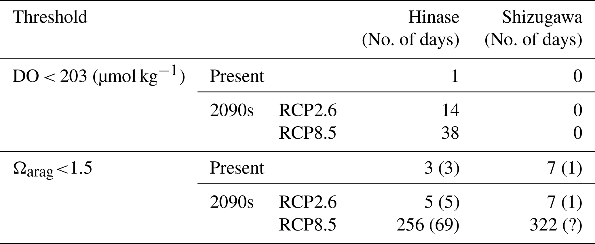
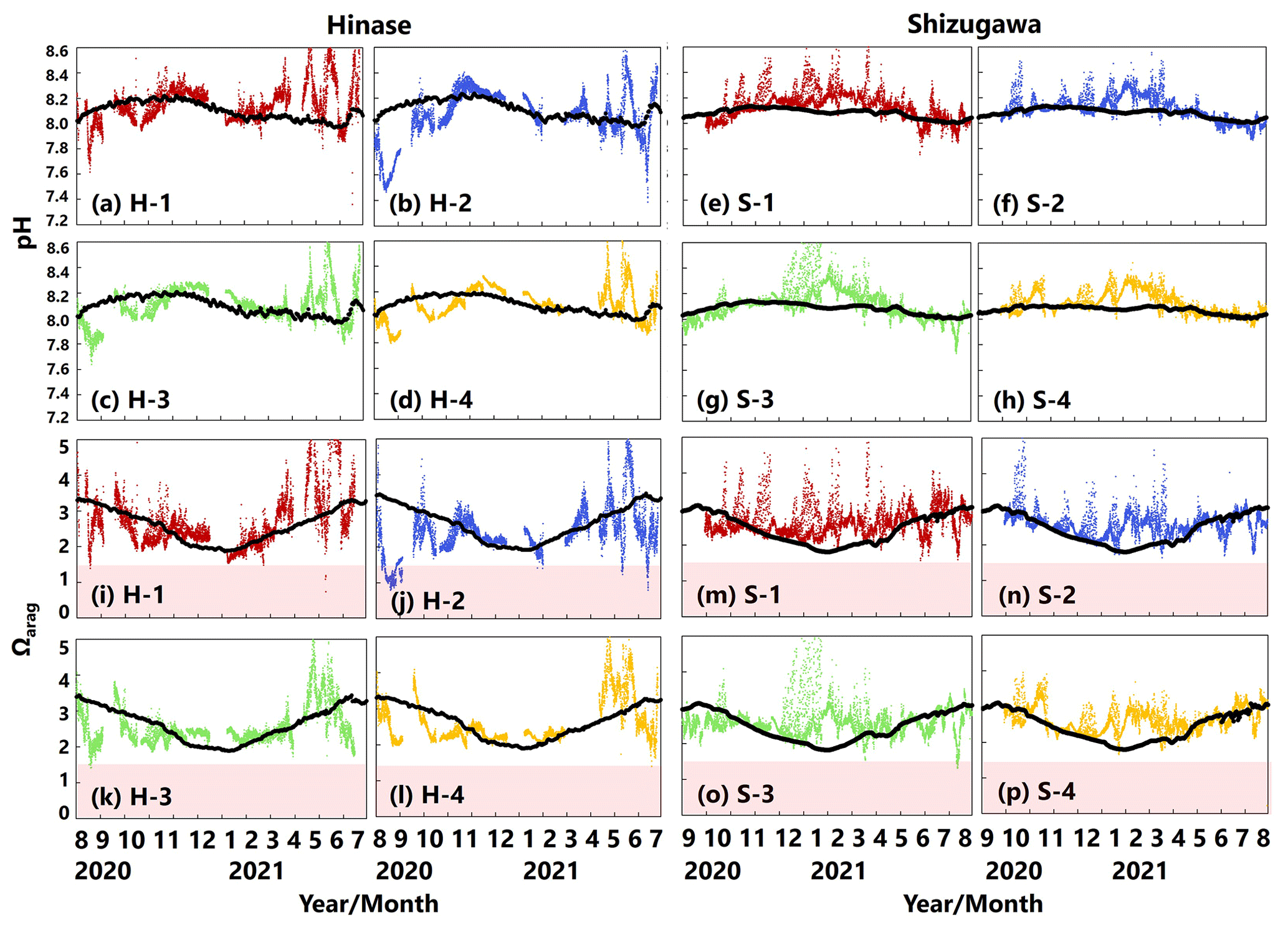
Figure 13 Observed (colored dots) and modeled (black lines) pH (a–h) and Ω_arag (i–p) at 1 m depth in Hinase (August 2020 to July 2021) and Shizugawa (September 2020 to August 2021). Red domains denote the critical level of acidification for Pacific oyster larvae in Waldbusser et al. (2015) (Ω_arag<1.5).

Following previous studies (e.g., Hauri et al., 2013; DeJong et al., 2015; Wada et al., 2020), monthly-mean contributions of pH and Ω_arag changes (ΔpH and ΔΩ_arag, respectively) with temperature (∂pH $/$ $\partial T\cdot \mathrm{\Delta }T$ and ∂Ω_arag $/$ $\partial T\cdot \mathrm{\Delta }T$), A_T (∂pH $/$ $\partial A_{\mathrm{T}}\cdot \mathrm{\Delta }\mathrm{nTA}$ and $\partial {\mathrm{\Omega }}_{\mathrm{arag}}/\partial A_{\mathrm{T}}$ ⋅ ΔnA_T), DIC (∂pH $/$ ∂DIC ⋅ ΔnDIC and ∂Ω_arag $/$ ∂DIC ⋅ ΔnDIC), and salinity (ΔFSpH and ΔFSΩ_arag) during the study period were examined. The contribution of ΔpH and ΔΩ_arag in each parameter is expressed as follows, based on Hauri et al. (2013):

$$\begin{array}{}\text{(4)}& \mathrm{\Delta }\mathrm{pH}\cong {\displaystyle \frac{\partial \mathrm{pH}}{\partial T}}\mathrm{\Delta }T+{\displaystyle \frac{\partial \mathrm{pH}}{\partial A_{\mathrm{T}}}}\mathrm{\Delta }n{A}_{\mathrm{T}}+{\displaystyle \frac{\partial \mathrm{pH}}{\partial \mathrm{DIC}}}\mathrm{\Delta }n\mathrm{DIC}+\mathrm{\Delta }{\mathrm{FS}}_{\mathrm{pH}}\end{array}$$

and

$$\begin{array}{}\text{(5)}& \begin{array}{rl}\mathrm{\Delta }{\mathrm{\Omega }}_{\mathrm{arag}}& \cong {\displaystyle \frac{\partial {\mathrm{\Omega }}_{\mathrm{arag}}}{\partial T}}\mathrm{\Delta }T+{\displaystyle \frac{\partial {\mathrm{\Omega }}_{\mathrm{arag}}}{\partial A_{\mathrm{T}}}}\mathrm{\Delta }n{A}_{\mathrm{T}}+{\displaystyle \frac{\partial {\mathrm{\Omega }}_{\mathrm{arag}}}{\partial \mathrm{DIC}}}\mathrm{\Delta }n\mathrm{DIC}\\ & +\mathrm{\Delta }{\mathrm{FS}}_{{\mathrm{\Omega }}_{\mathrm{arag}}},\end{array}\end{array}$$

where

$$\begin{array}{}\text{(6)}& \mathrm{\Delta }{\mathrm{FS}}_{\mathrm{pH}}={\displaystyle \frac{\partial \mathrm{pH}}{\partial S}}\mathrm{\Delta }S+{\displaystyle \frac{\partial \mathrm{pH}}{\partial A_{\mathrm{T}}}}\mathrm{\Delta }{A_{\mathrm{T}}}^S+{\displaystyle \frac{\partial \mathrm{pH}}{\partial \mathrm{DIC}}}\mathrm{\Delta }{\mathrm{DIC}}^S\end{array}$$

and

$$\begin{array}{}\text{(7)}& \mathrm{\Delta }{\mathrm{FS}}_{{\mathrm{\Omega }}_{\mathrm{arag}}}={\displaystyle \frac{\partial {\mathrm{\Omega }}_{\mathrm{arag}}}{\partial S}}\mathrm{\Delta }S+{\displaystyle \frac{\partial {\mathrm{\Omega }}_{\mathrm{arag}}}{\partial A_{\mathrm{T}}}}\mathrm{\Delta }{A_{\mathrm{T}}}^S+{\displaystyle \frac{\partial {\mathrm{\Omega }}_{\mathrm{arag}}}{\partial \mathrm{DIC}}}\mathrm{\Delta }{\mathrm{DIC}}^S.\end{array}$$

ΔnA_T and ΔnDIC are the salinity-normalized deviations from the annual means of A_T and DIC during the study period. $\mathrm{\Delta }{A_{\mathrm{T}}}^S$ and ΔDIC^S are deviations from the annual means due to freshwater input, and ΔFS_pH and $\mathrm{\Delta }{\mathrm{FS}}_{{\mathrm{\Omega }}_{\mathrm{arag}}}$ are the total contributions of freshwater input to ΔpH and ΔΩ_arag, respectively (Hauri et al., 2013).

ΔpH in Hinase was primarily controlled by ∂pH $/$ $\partial T\cdot \mathrm{\Delta }T$; i.e., pH was enhanced by warmer temperature in summer and autumn and was lowered by cooler temperature in winter and spring (Fig. 14a). Contribution of ∂pH $/$ ∂DIC ⋅ ΔDIC, resulting from biological production, was also dominant but the phase of ∂pH $/$ ∂DIC ⋅ ΔDIC was 4–5 months different from that of ∂pH $/$ ∂T ⋅ ΔT. The two terms partly canceled each other out and formed ΔpH. ΔpH in Shizugawa, on the other hand, was primarily controlled by ∂pH $/$ ∂DIC ⋅ ΔDIC, and the contribution of ∂pH $/$ ∂DIC ⋅ ΔDIC was largely canceled out by that of ∂pH $/$ ∂T ⋅ ΔT, which is out of phase in most of the months (Fig. 14b). As a result, ΔpH was relatively small in Shizugawa.

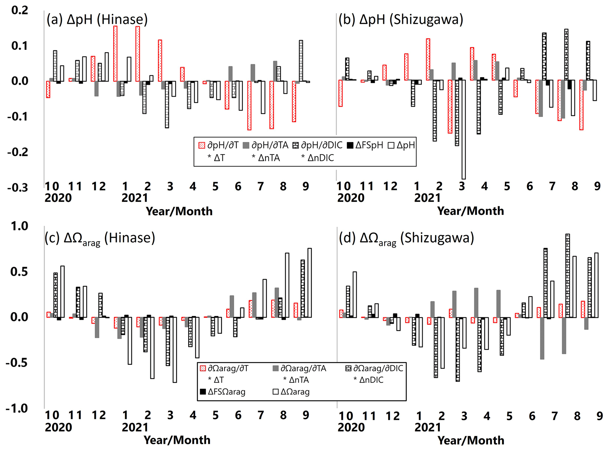
Figure 14 Monthly-mean contributions of pH and Ω_arag changes (ΔpH, a–b; ΔΩ_arag, c–d) in temperature (∂pH $/$ ∂T ⋅ ΔT and ∂Ω_arag/∂T ⋅ ΔT), A_T (∂pH $/$ ∂A_T ⋅ ΔA_T and $\partial {\mathrm{\Omega }}_{\mathrm{arag}}/\partial A_{\mathrm{T}}$ ⋅ ΔA_T), DIC (∂pH $/$ ∂DIC ⋅ ΔDIC and $\partial {\mathrm{\Omega }}_{\mathrm{arag}}/\partial$DIC ⋅ ΔDIC), and salinity (ΔFSpH and ΔFSΩ_arag) in Hinase (at H-4; a, c) and in Shizugawa (at S-4; b, d).

ΔΩ_arag values in Hinase and Shizugawa were primarily controlled by ∂pH $/$ ∂DIC ⋅ ΔnDIC and ∂Ω_arag/∂DIC ⋅ ΔnDIC; that is, pH and Ω_arag were enhanced by lower DIC concentration in winter and spring and lowered by higher DIC concentration in summer and autumn (Fig. 14c–d). The difference between ΔpH and ΔΩ_arag is that ΔpH was mainly controlled by temperature and DIC changes, while ΔΩ_arag was primarily controlled by DIC and A_T changes. The phases of ∂pH $/$ ∂A_T ⋅ ΔnA_T and $\partial {\mathrm{\Omega }}_{\mathrm{arag}}/\partial A_{\mathrm{T}}$ ⋅ ΔnA_T were almost opposite in the study period and, therefore, contributed to ΔpH and ΔΩ_arag differently between Hinase and Shizugawa. The monthly-mean contributions of ΔFS_pH and $\mathrm{\Delta }{\mathrm{FS}}_{{\mathrm{\Omega }}_{\mathrm{arag}}}$ to ΔpH and ΔΩ_arag were minor.

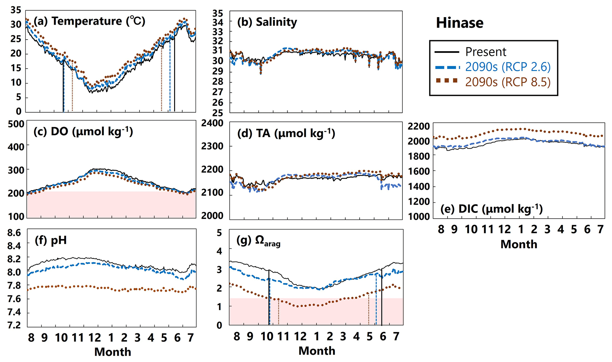
Figure 15 Modeled (a) temperature (^∘C), (b) salinity, (c) DO (µmol kg⁻¹), (d) A_T (µmol kg⁻¹), (e) DIC (µmol kg⁻¹), (f) pH, and (g) Ω_arag values in Hinase from August to July currently (solid black lines) and in the 2090s (RCP2.6 scenario, dashed blue lines; RCP8.5 scenario, dotted brown lines). The red domain in (c) denotes DO concentrations below the optimum DO range (< 203 µmol kg⁻¹) for the growth of Pacific oyster (Hochachka, 1980; Fisheries Agency, 2013). The red domain in (g) denotes the critical level of acidification for Pacific oyster larvae in Waldbusser et al. (2015) (Ω_arag<1.5). Modeled end and start dates of spawning period of Pacific oysters at present and in the 2090s with the RCP2.6 and RCP8.5 scenarios (Table 2) are shown in vertical solid black lines, dashed blue lines, and dotted brown lines, respectively, in (a) and (g). The end and start dates of the spawning period were estimated by referring to thresholds obtained from Oizumi et al. (1971).

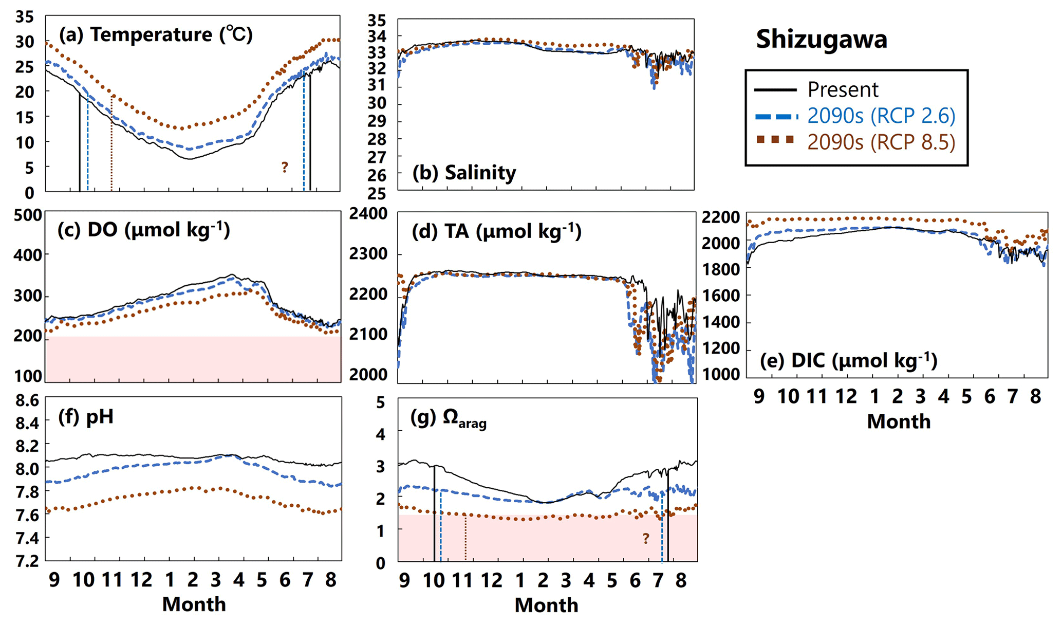
Figure 16 Modeled (a) temperature (^∘C), (b) salinity, (c) DO (µmol kg⁻¹), (d) A_T (µmol kg⁻¹), (e) DIC (µmol kg⁻¹), (f) pH, and (g) Ω_arag values in Shizugawa from September to August currently (solid black lines) and in the 2090s (RCP2.6 scenario, dashed blue lines; RCP8.5 scenario, dotted brown lines). The red domain in (c) denotes DO concentrations below the optimum DO range (< 203 µmol kg⁻¹) for the growth of Pacific oyster (Hochachka, 1980; Fisheries Agency, 2013). The red domain in (g) denotes the critical level of acidification for Pacific oyster larvae in Waldbusser et al. (2015) (Ω_arag<1.5). Modeled end and start dates of the spawning period of Pacific oysters at present and in the 2090s with the RCP2.6 and RCP8.5 scenarios (Table 2) are shown in vertical solid black lines, dashed blue lines, and dotted brown lines, respectively, in (a) and (g). The end and start dates of the spawning period were estimated by referring to thresholds obtained from Oizumi et al. (1971). The start date of the spawning season in the 2090s with the RCP8.5 scenario could not be projected in Shizugawa because water temperature lower than 10^∘C was not projected, and therefore, the threshold for evaluating the start date by Oizumi et al. (1971) could not be applied.

4 Discussion

4.1 Future projection

The projected results for physical and biogeochemical parameters in the 2090s differed markedly between Hinase and Shizugawa and between the RCP scenarios (RCP2.6 vs. RCP8.5) (Figs. 15 and 16).

In Hinase, the projected rise in water temperature for the rest of this century was slight (Fig. 15a), so DO concentrations will not change significantly (Fig. 15c). Similarly, salinity will not change by the end of this century, leading to no significant change in A_T (Fig. 15b, d). Therefore, the significant decrease in pH and Ω_arag values from the present to the 2090s, especially with the RCP8.5 scenario, is likely caused by the large increase in DIC resulting from the increased atmospheric CO₂ concentrations towards the end of the century (Fig. 15e). The projected results show that larvae of Pacific oysters (C. gigas) may experience a critical Ω_arag value year-round with the RCP8.5 scenario (Fig. 15g). This severe condition could be alleviated if anthropogenic CO₂ emissions are cut sufficiently in accordance with the Paris Agreement (RCP2.6 scenario). The projected results also imply no severe impact of deoxygenation on the growth of Pacific oysters, neither now nor in the 2090s, at least at 1 m depth.

In Shizugawa, water temperatures are predicted to rise by the 2090s (Fig. 16a), substantially decreasing DO concentrations (Fig. 16c). Although salinity and A_T values will not change from the present to the 2090s with any RCP scenario (Fig. 16b, d), DIC will increase significantly (Fig. 16e). Therefore, similarly to for Hinase, the Ω_arag value is predicted to decrease markedly towards the 2090s (Fig. 16g), mainly because of the increase in DIC values. In Shizugawa, no severe conditions for Pacific oysters are predicted with regard to DO concentrations, but Ω_arag values will be below the threshold (< 1.5) except in summer, unless anthropogenic CO₂ is reduced sufficiently.

4.2 Combined impacts of coastal warming, acidification, and deoxygenation

Because estimation of the timing of start and end dates of Pacific oyster (C. gigas) spawning is dependent on water temperature, the timing may be altered by future coastal warming. After confirming that the simulated timing of start and end dates is consistent with the observation-based estimated timing for the present, as described in Sect. 3.2, we projected the timing for the future.

Our model results imply that in Hinase the start date will be earlier in the 2090s than at present, by 2 weeks with the RCP2.6 scenario and by almost 1 month with the RCP8.5 scenario, and the end date will be later by around 20 d with the RCP8.5 scenario (Table 2; Fig. 15). In Shizugawa, the end date will be 10 d later than at present in the 2090s with the RCP2.6 scenario and more than 1 month later with the RCP8.5 scenario (Table 2; Fig. 16). With the RCP2.6 scenario, the start date is projected to be 10 d earlier in the 2090s than at present. With the RCP8.5 scenario, the water temperature is projected to be above 10^∘C year-round in the 2090s; therefore, we could not estimate the start date based on Oizumi et al. (1971).

Coastal warming and acidification may have synergistic impacts on Pacific oyster larvae. As mentioned above, coastal warming will lengthen the spawning period, which is the life stage most vulnerable to acidification. Therefore, Pacific oyster larvae may suffer from acidification more severely and over a longer period. Our model results imply that the number of days on which Ω_arag values are below the threshold of acidification for Pacific oyster larvae (1.5) in Hinase will increase from 0 d at present with the RCP2.6 scenario and to 204 d with the RCP8.5 scenario in the 2090s (Fig. 15). With the RCP8.5 scenario, 17 of the 204 d are during the spawning period. In Shizugawa, the number of days on which Ω_arag values are below 1.5 will increase from 0 d from the present with the RCP2.6 scenario to 244 d with the RCP8.5 scenario in the 2090s (Fig. 16).

However, because of the reasons mentioned in Sect. 2.4, the model underestimated the observed short-term fluctuation in Ω_arag (Fig. 13). Therefore, the number of days on which Ω_arag values are below 1.5 is also considered to be underestimated. Assuming that the observed short-term fluctuations in Ω_arag at present are maintained in the future, the simulated or projected number of days is increased from 0 to 3 d for the present, from 0 to 5 d with the RCP2.6 scenario, and from 204 to 256 d with the RCP8.5 scenario in Hinase. In Shizugawa, the projected number of days is modified from 0 to 7 d for the present with the RCP2.6 scenario and from 244 to 322 d with the RCP8.5 scenario (Table 3, Fig. S1). The duration of severe conditions might be 2 weeks longer, considering that 2–4 weeks is required for Pacific oyster larvae to settle after birth (e.g., Chanley and Dinamani, 1980; Tachi et al., 2013). The prolonged spawning period may shorten the oyster shipping period and lower their quality (Akashige and Fushimi, 1992), potentially damaging the oyster-processing industry.

Compared to the combined impacts of coastal warming and acidification, our model results indicate that the impact of deoxygenation on Pacific oysters will be less severe, at least in surface waters. The model results reveal that the number of days on which DO concentrations are below the optimal range for Pacific oyster growth (< 203 µmol kg⁻¹) will increase in Hinase from 1 d at present to 14 and 38 d in the 2090s with the RCP2.6 and RCP8.5 scenarios, respectively, and 0 d in Shizugawa at present and in the 2090s (Table 3). Similarly to for Ω_arag, however, the number of days on which DO concentrations are below 203 µmol kg⁻¹ is considered to be even greater if the observed significant short-term fluctuation (Fig. 10) is assumed. Nevertheless, we could not take the short-term fluctuation into account because of the lack of continuous DO observations (Fig. 11). Also, previous studies imply that impacts on marine organisms appear more severely under the co-occurrence of ocean acidification and deoxygenation than the occurrence of each stressor alone (Steckbauer et al., 2020; Yorifuji et al., 2023). In other words, the threshold for deoxygenation alone (203 µmol kg⁻¹) could be higher in the future when ocean acidification progresses.

4.3 Thresholds for impacts of ocean acidification on Pacific oysters on Japan coasts

In this study, impacts of ocean acidification on Pacific oysters (C. gigas) were evaluated by using the threshold of Ω_arag=1.5 (Waldbusser et al., 2015). On the other hand, as mentioned in Sect. 3.1, by microscopic examination we did not observe any morphological abnormalities in the larvae (Fig. 7), and therefore, we did not find any anecdotal evidence of impacts of ocean acidification on Pacific oyster larvae in this study. This is different from the situation on the West Coast of the USA where oyster farms have already been reported to be impacted by low-pH, low-Ω_arag seawater (e.g., Barton et al., 2012), as mentioned in Sect. 1. We need to clarify the discrepancy between the scientific findings and the fact that no specific impacts of ocean acidification on Pacific oyster larvae have so far been detected in the study sites, even though they occasionally experience the critical level of ocean acidification proposed by a previous study (Ω_arag<1.5; Waldbusser et al., 2015).

It is possible that we failed to collect abnormal larvae samples for the reason that the abnormal larvae died before our samples were taken, although it is unlikely that there were many such abnormal larvae present. If so, the plankton nets would have been able to collect sufficient numbers of them to be detected under microscopic examination.

Rearing experiments of Waldbusser et al. (2015) were performed in Oregon, USA, where Pacific oysters are not native, while they are native in both the Hinase area and Shizugawa Bay. Therefore, it is possible that the Pacific oysters in Hinase and Shizugawa have already partly adapted to local environmental changes, including lower-pH and lower-Ω_arag conditions caused by riverine discharge of freshwater and organic matter. To verify this, we might need further examination including new rearing experiments for native Pacific oyster species on Japan coasts.

Previous studies also suggest that oyster larvae have decreased swimming ability and sink as salinity decreases (e.g., Dekshennieks et al., 1996). Therefore, it is possible that the Pacific oyster larvae did not remain in low-salinity waters and consequently could escape from the lower-pH and lower-Ω_arag conditions. These issues should be taken into consideration in future works, although they are not in this study, and therefore, the impacts of ocean acidification on Pacific oysters may have been overestimated in this sense. Also, considering that our current model underestimated observed sudden decreases in salinity as mentioned in Sect. 3.2, more realistic input data of freshwater from rainfall and riverine water would be necessary for better model performance.

5 Conclusions

Impacts of ongoing coastal warming, acidification, and deoxygenation on Pacific oysters on Japan coasts have not been clarified before. This study aimed to assess the current impacts and project the future impacts, through continuous monitoring, microscopic examination, and numerical modeling in two representative oyster-farming regions in Japan, the Hinase area and Shizugawa Bay. This study first elucidated that oyster-farming sites in Hinase have experienced critical levels of acidification, although Pacific oyster larvae do not seem to have been affected. It may therefore be necessary to revisit the acidification threshold for Pacific oysters farmed on Japan coasts.

Our future projections imply that unless CO₂ emissions are reduced in accordance with the Paris Agreement (RCP2.6 scenario), oyster farming at the study sites may be seriously affected by coastal warming and acidification by the end of this century. The greatest impact will be on larvae, as a result of longer exposure to more acidified waters. A prolonged spawning period may harm oyster processing by shortening the shipping period and reducing oyster quality. Therefore, to minimize impacts on Pacific oyster farming, in addition to mitigation measures, local adaptation measures – such as regulation of freshwater and organic matter inflow from rivers and changes in oyster-farming practices – may be required.

Climate-change-driven extreme events will cause more frequent and intense heavy rainfall; subsequent river inflow of freshwater and organic matter to coasts may further reduce pH and Ω_arag in oyster farms. To plan how to minimize the adverse impacts of coastal warming and acidification, coupled physical–biogeochemical models with higher spatiotemporal resolution are needed to simulate river-inflow processes and daily fluctuations in biogeochemical parameters.