the Creative Commons Attribution 4.0 License.
the Creative Commons Attribution 4.0 License.
 | 24 Nov 2023
Chromophoric dissolved organic matter dynamics revealed through the optimization of an optical–biogeochemical model in the northwestern Mediterranean Sea
Eva Álvarez
Gianpiero Cossarini
Anna Teruzzi
Jorn Bruggeman
Karsten Bolding
Stefano Ciavatta
Vincenzo Vellucci
Fabrizio D'Ortenzio
David Antoine
Paolo Lazzari
Chromophoric dissolved organic matter (CDOM) significantly contributes to the non-water absorption budget in the Mediterranean Sea. The absorption coefficient of CDOM, aCDOM(λ), is measurable in situ and can be retrieved remotely, although ocean-colour algorithms do not distinguish it from the absorption of detritus. These observations can be used as indicators for the concentration of other relevant biogeochemical variables in the ocean, e.g. dissolved organic carbon. However, our ability to model the biogeochemical processes that determine CDOM concentrations is still limited. Here we propose a novel parameterization of the CDOM cycle that accounts for the interplay between the light- and nutrient-dependent dynamics of local CDOM production and degradation, as well as its vertical transport. The parameterization is included in a one-dimensional (1D) configuration of the Biogeochemical Flux Model (BFM), which is here coupled to the General Ocean Turbulence Model (GOTM) through the Framework for Aquatic Biogeochemical Models (FABM). Here the BFM is augmented with a bio-optical component that resolves spectrally the underwater light transmission. We run this new GOTM-(FABM)-BFM configuration to simulate the seasonal aCDOM(λ) cycle at the deep-water site of the Bouée pour l'acquisition de Séries Optiques à Long Terme (BOUSSOLE) project in the northwestern Mediterranean Sea. Our results show that accounting for both nutrient and light dependence of CDOM production improves the simulation of the seasonal and vertical dynamics of aCDOM(λ), including a subsurface maximum that forms in spring and progressively intensifies in summer. Furthermore, the model consistently reproduces the higher-than-average concentrations of CDOM per unit chlorophyll concentration observed at BOUSSOLE. The configuration, outputs, and sensitivity analyses from this 1D model application will be instrumental for future applications of BFM to the entire Mediterranean Sea in a three-dimensional configuration.
- Article
(11870 KB) - Full-text XML
- BibTeX
- EndNote


The inventory and composition of dissolved organic matter (DOM) is of utmost importance to marine ecosystems as it is the energy base and carbon source for heterotrophic life in the ocean (Azam et al., 1983). Furthermore, as the largest pool of reduced carbon in the oceans, DOM plays an important role in the global carbon cycle (Legendre et al., 2015). Although most of the dissolved exudates that form the DOM are non-light-absorbing (Mühlenbruch et al., 2018), part of the pool absorbs light mainly in the ultraviolet (UV) and blue spectral range of the electromagnetic radiation. This portion of the DOM is referred to as chromophoric dissolved organic matter (CDOM, Jerlov, 1951; Sieburth and Jensen, 1968). CDOM absorbs light depending on both the CDOM concentration and its mass-specific spectral absorption coefficient. aCDOM(λ) is a measurable proxy for fundamental processes regulating CDOM dynamics. The high absorption of CDOM in the blue part of the electromagnetic spectrum affects the water leaving radiance, a radiometric quantity that can be retrieved by satellites, and interferes with estimates of chlorophyll a concentration (Chl a) from ocean-colour observations (Siegel et al., 2013). This is particularly important for the Mediterranean Sea because its surface waters (0–20 m) appear greener than the global ocean, although its phytoplankton concentration is typically lower (Chl a<0.2 mg m−3) (Morel and Gentili, 2009b; Claustre et al., 2002; Volpe et al., 2007). Besides the presence of CDOM, there are other possible factors influencing this optical behaviour, including the particular pigment ratios in the Mediterranean phytoplankton community (Organelli et al., 2011), the abundance of small coccolithophores (Gitelson et al., 1996), and the influence of Saharan dust (Claustre et al., 2002). However, the high contribution of CDOM was found to be a major factor since the CDOM concentration in the basin is about twice that in the Atlantic at the same latitudes (Morel and Gentili, 2009b).
aCDOM(λ) can be measured in situ at selected locations and can be retrieved on a global scale from remote-sensing platforms, although remotely it is not distinguishable from the absorption of detritus. Remote-sensing platforms provide radiometric observations, which are used to compute a combined value for the absorption coefficient of CDOM and of detritus, aDG(λ) (Werdell et al., 2018). On the other hand, spectrally resolved biogeochemical (BGC) models provide aCDOM(λ) estimates by simulating CDOM concentrations and prescribing the optical properties of the pool. Such BGC–optical models could advance the understanding of the dynamics shaping aCDOM(λ). However, they rely on the accurate representation of both the dynamics of CDOM cycling and its optical properties. CDOM cycling is essentially controlled by in situ biological production (Romera-Castillo et al., 2010), terrestrial and atmospheric sources and physical transport, microbial consumption (Nelson and Gauglitz, 2016; Legendre et al., 2015; Stedmon and Markager, 2005), and deep ocean circulation and/or vertical mixing (Coble, 2007), and it is photoreactive and efficiently destroyed in the upper layers of the water column by solar radiation (Mopper and Kieber, 2000). Most marine ecosystem models that explicitly resolve CDOM follow Bissett et al. (1999) (e.g. Xiu and Chai, 2014; Dutkiewicz et al., 2015), in which CDOM is assumed to have a source that is a fixed fraction of the dissolved primary production (dpp) of phytoplankton, is remineralized slowly, and is bleached under high-light conditions. These formulations seem to work well in open waters (Dutkiewicz et al., 2015) but not in the northwestern (NW) Mediterranean Sea, where CDOM is not a constant proportion of dpp, even when co-varying with phytoplankton Chl a (Lazzari et al., 2021b). The aim of this work is to decipher the processes that influence CDOM dynamics in the NW Mediterranean Sea by advancing and using a BGC–optical model in synergy with in situ observations.
A major challenge in modelling CDOM concentrations in the Mediterranean Sea concerns the origin of the CDOM pool in superficial waters – i.e. how large is the proportion of CDOM transported from allochthonous sources compared to CDOM produced locally by primary and secondary production (Santinelli et al., 2002; Copin-Montégut and Avril, 1993)? In the basin, the higher-than-average CDOM concentrations seem to be sustained by allochthonous sources as fluxes of DOM depositions from the atmosphere are 2–5 times larger in the Mediterranean Sea than those estimated for the global ocean, which explains the abundance of humic-like substances (Santinelli, 2015; Galletti et al., 2019). Therefore, accurate modelling of the balance between CDOM transport (atmospheric input, advection, and/or vertical replenishment from deeper stocks) and destruction at the surface (photolysis and bacterial consumption) is crucial to accurately represent the role of CDOM of allochthonous origin in shaping the dynamics of aCDOM(λ) in the NW Mediterranean Sea.
As for locally produced CDOM, the challenge is that the mechanisms for CDOM production and destruction involve processes that are decoupled from phytoplankton dpp, such as photolysis, zooplankton sloppy feeding, and bacterial production and consumption. In the open waters of the NW Mediterranean Sea, far from terrestrial inputs, photobleaching and biological production and consumption are suggested to be important factors determining the seasonality of aCDOM(λ) (Pérez et al., 2016; Xing et al., 2014; Organelli et al., 2014). aCDOM(λ) and Chl a concentration roughly covary at the surface, but the causative mechanisms are different. While aCDOM(λ) dynamics at the surface are mainly explained by vertical transport of CDOM from depth and by photochemical destruction, Chl a concentration at the surface is mainly driven by photoacclimation of phytoplankton and nutrient limitation. There is also a close coupling between subsurface aCDOM(λ) and phytoplankton Chl a via microbial activities or interactions in the planktonic food web (Pérez et al., 2016; Xing et al., 2014; Organelli et al., 2014), although the relative contribution to CDOM production by phytoplankton and by bacteria is still controversial (Romera-Castillo et al., 2010). Although it is generally assumed that phytoplankton in open oceans are not a direct source of CDOM but rather a source of labile organic matter that is microbially transformed and subsequently produces CDOM (Nelson et al., 1998; DeGrandpre et al., 1996), observations in the NW Mediterranean Sea suggest direct CDOM production by phytoplankton (Oubelkheir et al., 2007, 2005; Xing et al., 2014). Therefore, to incorporate CDOM in an ecosystem model of the NW Mediterranean Sea, one must consider the composition of DOM produced by phytoplankton in addition to the cycling of dissolved matter and the microbial loop in the area.
We approached this challenge by using the Biogeochemical Flux Model (BFM, Vichi et al. 2007) in a one-dimensional (1D) configuration. The BFM was coupled to the General Ocean Turbulence Model (GOTM, Burchard et al., 1999), a 1D water column turbulent kinetic energy model, by using the Framework for Aquatic Biogeochemical Models (FABM, Bruggeman and Bolding, 2014). In such a configuration, the model accounts for the vertically differentiated processes of photobleaching and transport from deep inventories. Local CDOM production includes the excretion of phytoplankton, which depends on light and nutrient availability, the bacterial production and consumption, and zooplankton activities. The version of BFM used here resolves the spectral light transmission underwater (Terzić et al., 2021; Lazzari et al., 2021a) and simulates the inherent optical properties (IOPs) of CDOM, phytoplankton, and organic detritus in the water column. The model output can be compared with a range of optical observations made in the field and remotely.
With this model configuration, we simulated a data-rich monitoring site in the NW Mediterranean. The Bouée pour l'acquisition de Séries Optiques à Long Terme (BOUSSOLE) observatory is located in the Ligurian Sea, about 32 nautical miles off the French coast (Antoine et al., 2006). In this area, the water depth varies between 2350 and 2500 m, and the currents are extremely slow. This peculiarity is due to its location near the centre of the cyclonic circulation that characterizes the Ligurian Sea, and it makes reasonable the approximation of a 1D configuration. The BOUSSOLE observatory consists of a mooring where a buoy, specifically designed for collecting radiometric and bio-optical quantities, collects optical data at a high temporal resolution. Oceanographic cruises visit the site monthly to collect a complementary dataset of algal pigment concentrations and IOPs, which include light absorption coefficients of phytoplankton, detritus, and CDOM (Antoine et al., 2006). Numerous studies combining optics and biochemistry have exploited these two complementary sets of observations collected at the BOUSSOLE site, e.g. fluorescence to infer Chl a (e.g. Bayle et al., 2015; Mignot et al., 2011) and phytoplankton community composition (Sauzède et al., 2015), to infer the size structure of the phytoplankton community from measured light spectra (Organelli et al., 2013), and to estimate community production from particle backscattering coefficients (Barbieux et al., 2022; Barnes and Antoine, 2014). One-dimensional models developed or employed at the BOUSSOLE site have focused separately on physics and biochemistry (e.g. D'Ortenzio et al., 2008; Ulses et al., 2016) or optics (Blum et al., 2012), but to our knowledge, no spectrally resolved BGC model has been used previously to simulate the site.
Methods that merge models and observations can make significant progress in reducing model uncertainty (e.g. Teruzzi et al., 2021; Ciavatta et al., 2018), and data-intensive processes such as model calibration and validation are of utmost importance to make model applications reliable (Arhonditsis and Brett, 2004). A major challenge when working with complex coupled hydrodynamic–BGC numerical models is the need to make an appropriate choice of model parameter values that ensure optimal performance in terms of reproducing observational data. Genetic algorithms are commonly used by BGC modellers to solve nonlinear optimization problems such as parameter estimation (e.g. Kriest et al., 2017; Kuhn and Fennel, 2019; Falls et al., 2022; Wang et al., 2020; Mattern and Edwards, 2017). In this work, we calibrated the model by using the Parallel Sensitivity Analysis and Calibration utility (ParSAC, Bruggeman and Bolding, 2020), which implements the Differential Evolution (DE) algorithm (Storn and Price, 1997). The DE algorithm is a stochastic, population-based, and direct-search parallel method which operates through genetic operations, namely mutation, crossover, and selection. Its objective is to eventually guide the population to the most likely values of model parameters based on the agreement of model output with observations.
With these three elements, (i.e. the 1D hydrodynamic–BGC–optical model GOTM-(FABM)-BFM, the observations collected at BOUSSOLE, and the optimization tool), here, we propose and optimize a novel formulation for the simulation of CDOM at the BOUSSOLE site. The specific objective of the present study is to improve the representation of the variability of aCDOM(λ) within a coupled BGC–optical model of the ocean by (i) linking biodegradable CDOM produced by phytoplankton to both nutrient availability and light intensity and (ii) improving the representation of the sources of allochthonous CDOM. We optimized optical and BGC parameters to improve the representation of the observed variables at the BOUSSOLE site and investigated the model simulation of the unobserved variables (e.g. DOC, bacterial concentration) and bio-optical relationships between aCDOM(λ) and Chl a and DOC. Based on the optimized model configuration, we conducted two numerical experiments to gain new insights into (i) the BGC processes that determine the seasonal dynamics of CDOM at the surface and at the depth of the Chl a maximum (DCM) and (ii) the role of local production versus allochthonous inputs in the total pool of CDOM.
The model tested in the present work is a one-dimensional (depth) configuration of the BFM, extended here with a bio-optical component, as described in Sect. 2.1. The observational data, which are explained in detail in Sect. 2.2, come from the BOUSSOLE project. A test case of the BOUSSOLE site in the NW Mediterranean from the surface to 2400 m is used, and the setup of the site is described in Sect. 2.3. The optimization strategy is described in Sect. 2.4, which also outlines the details of the experiments.
2.1 Model description
The modelling framework consisted of four elements: (i) a hydrodynamic model that simulates the vertical mixing of BGC variables, (ii) a coupling layer that connects the hydrodynamic model to the BGC model, (iii) a BGC model that simulates the sink and source terms of BGC variables, and (iv) a bio-optical model that resolves the underwater field of spectral light based on the presence of optical constituents in the water column.
2.1.1 The hydrodynamic model GOTM and the framework FABM
The General Ocean Turbulence Model (GOTM, Burchard et al., 1999) is a one-dimensional water column built around an extensive library of turbulence closure models. GOTM is very configurable and simulates the vertical structure of the water column – notably saline, thermal and turbulence dynamics. Being a 1D model, horizontal gradients at the application sites need to be either negligible or parameterized. A key advantage of a 1D model is that it is feasible to make long simulations with high vertical resolution as the computational resources required are much smaller compared to full 3D models. The open-source, Fortran-based Framework for Aquatic Biogeochemical Models (FABM, Bruggeman and Bolding, 2014) provides a coupling layer that enables the flexible coupling of ecosystem processes into the GOTM. FABM enables complex BGC models to be developed as sets of stand-alone, process-specific modules. These are combined at runtime through coupling links to create a custom-made BGC–ecosystem model. At each simulation time step, the BGC equations are applied to each layer, and the rates of sink and source terms are calculated at the current time and in the current space using local variables (e.g. light, temperature, and concentrations of state variables) provided by the GOTM. The rates pass to the hydrodynamic model via FABM, which handles numerical integration of the BGC processes and the transport of BGC substances (e.g. nutrients, dissolved and particulate organic matter) between the layers. Updated states are then passed back to the BGC model via FABM.
The implementation of the BFM in FABM comprises 54 state variables. These include representations of dissolved inorganic carbon (O(DIC)); inorganic forms of nitrogen (; ammonium (; phosphorus ( and silicate (N(Si)); four phytoplankton types (P(DIATOM), P(NANO), P(PICO), and P(DINO)); heterotrophic bacteria (B) and four grazers (Z(HETEN), Z(MICRO), Z(OMNI), and Z(CARNI)); particulate organic matter (R(DET)), three pools of dissolved organic matter differentiated by reactivity into labile (R(1)), semi-labile (R(2)), and semi-refractory (R(3)); and CDOM differentiated by the same reactivities (X(1), X(2) and X(3)). In the following, subscripts are appended to the symbols for the components to indicate the elemental constituent for which the state variable stands, including carbon (C), nitrogen (N), phosphorus (P), Chl a (only in phytoplankton), and silica (Si, only in P(DIATOM)). In the spectrally resolved version of BFM used in this work, the transmission of light in the water column is resolved in 33 wavebands centred from 250 to 3700 nm, with 25 nm spectral resolution within the visible range (Terzić et al., 2021; Lazzari et al., 2021a). Vertically resolved irradiance is absorbed and scattered by water, phytoplankton, CDOM, and detritus. Although the code implementation involved a redesign of the BFM code into a FABM-compliant modular structure, the core of the overall conceptual model of the spectrally resolved BFM remains intact compared to previous applications (e.g. Lazzari et al., 2021b; Álvarez et al., 2022) and is described below. The sources for the code of GOTM, FABM, and the spectrally resolved BFM adapted to work under the FABM convention can be found in the “Code availability” section.
2.1.2 The BGC model BFM and the bio-optical component
A complete record of the partial differential equations for each state variable that conform to BFM can be found in several publications (Vichi et al., 2007a, b) along with the details of the spectrally resolved version (Terzić et al., 2021; Lazzari et al., 2021a). The following sections describe the main dynamics of the cycling of phytoplankton functional types (PFTs), DOC and CDOM, the optical treatment of constituents (PFTs, CDOM, and detritus), and the solution for light transmission. Following Vichi et al. (2007), the dynamical equations are written in “rate of change” form, where the right-hand side contains the terms representing significant processes for each living or non-living component. For each process, the state variable subject to change appears in front of a vertical bar, and the superscript and subscript after the bar are the three-letter acronym of the process represented and the state variable involved in the process, respectively.
Cycling of BGC variables: PFTs, DOC, and CDOM
Primary producers are divided into four types that roughly represent the functional spectrum of phytoplankton in marine systems: diatoms (P(DIATOM)), nanoflagellates (P(NANO)), picophytoplankton (P(PICO)), and dinoflagellates (P(DINO)). The variation in carbon concentration (mg C m−3 d−1), being i of each of the PFTs, is calculated as follows:
Here, we briefly describe spectrally resolved gross (gpp) and dissolved primary production (dpp), whereas the exact formulations for the respiration (rsp) and grazing (grz) processes can be found in the BFM manual (Vichi et al., 2020). Gross primary production of each phytoplankton species (mg C m−3 d−1) is computed as follows:
where is the maximum productivity rate (d−1), regulated by dimensionless temperature- (ftP(T)) and nutrient-dependent (fnP(nutrients)) factors. Growth-limiting nutrients are , , and N(Si) for P(DIATOM) and and for the rest of the phytoplankton types. Light regulates gpp through an increasing, saturating function of the number of photons absorbed per Chl a unit, the photochemical efficiency (ϕ, mg C µE−1) and the Chl a (-to-carbon ( ratio (θ, mg Chl a mg C−1). Total absorbed irradiance is the integral of the Chl a-specific absorption spectrum of photosynthetic pigments [] times E0(λ) (see Sect. 2.1.2.3 and Eq. 26) between 387.5 and 800 nm (µmol quanta mg Chl a−1 d−1). The photoacclimation term used in the calculation of is resolved spectrally in the same way, and the exact formulation can be found in Álvarez et al. (2022).
DOC in the BFM is characterized by reactivity into labile (, semi-labile (, and semi-refractory (, and, accordingly, CDOM is represented by the same three reactivity levels (, , and . CDOM is calculated as a fraction of the DOC produced by phytoplankton that only produce , zooplankton that only produce , and bacteria that only produce (green lines in Fig. 1, all in mg C m−3 d−1).
With respect to the semi-labile DOC produced by phytoplankton (, the BFM considers two components: (i) a constant percentage of carbon fixed by phytoplankton is lost from cells each day, along with dissolved organic phosphorus and nitrogen (DOP and DON, respectively), and (ii) photosynthetic overflow under conditions of nutrient limitation leads to the loss of photosynthesized carbon, which cannot be assimilated into biomass due to the absence of other nutrients. Following Thornton's (2014) definitions, the first process is defined as the passive leakage of molecules through the cell membrane, and the second process of exudation is defined as the loss of excess carbon due to changes in environmental conditions such as nutrient availability. Thus, the total amount of phytoplankton dpp in the BFM is a dynamic term that changes in response to environmental conditions and is calculated as follows:
where the first addend in the right-hand side of Eq. (3) represents the passive leakage of molecules across the cell membrane and is considered to be a fraction (βP) of the gpp, and the second addend represents the difference between the carbon assimilated into biomass (GP) and the total photosynthesized carbon in the case of intracellular nutrient deficiency (. For each PFT, GP(i) is calculated as gpp minus dpp and rsp, and is calculated as follows:
where and are the minimum phosphorous and nitrogen quota, respectively, and the two nitrogen sources are and . The exact formulations for the processes of phosphorous and nitrogen compounds uptake (upt) can be consulted in Vichi et al. (2020).
To investigate what fraction of these two fluxes is chromophoric and whether this proportion varies with environmental conditions, we included light and nutrient dependencies on phytoplankton CDOM production. Assuming that modelled exudation is dominated by non-chromophoric carbohydrates, under decreasing conditions of nutrient availability where exudation accounts for a larger proportion of dpp, the simulated proportion of chromophoric material in total dpp decreases. On the other hand, with a modelled leakage that contains more chromophoric material when cells have a higher intracellular pigment concentration, the simulated chromophoric fraction of the total dpp increases with decreasing light availability. Thus, whereas the DOC that leaked constantly from phytoplankton cells is considered to have an amount that is chromophoric and proportional to cell pigmentation (, DOC exuded under intra-cellular nutrient shortage is considered to be non-absorbing, and therefore it is not partitioned into CDOM. The coloured fraction of the total DOC of phytoplankton origin ( is the sum of all coloured material produced by PFTs with respect to total DOC production. The coloured fraction produced by each phytoplankton type i ( depends on the relative proportions of DOC that originated through leakage or exudation and on the intracellular concentration of Chl a as follows:
The non-absorbing part of this flux (1- is directed to the state variable and consumed by bacteria (upt):
CDOM is directed to the state variable , consumed by bacteria (upt), and photobleached (deg):
The formulations for the processes of bacterial consumption (upt) can be consulted in Vichi et al. (2020).
Labile DOC ( is produced by the excretion of microzooplankton (Z(MICRO)) and nano-heterotrophs (Z(HETEN)) (exc) and therefore represents the sources of DOC associated with the zooplankton-mediated mortality of phytoplankton and bacteria, and it is consumed quickly by bacteria. The released fraction of carbon by mesozooplankton excretion (both Z(OMNI) and Z(CARNI)), on the other hand, is assumed to have no dissolved products and is therefore directed to the state variable .
Labile CDOM ( is explicitly resolved as a constant fraction of exc determined by the parameter for microzooplankton and for nano-heterotrophs:
The formulations for the processes of zooplankton excretion (exc) can be consulted in Vichi et al. (2020).
The production of DOC by phytoplankton and as a by-product of zooplankton activities is an important driver of secondary production by heterotrophic prokaryotes. Labile and semi-labile DOC, both non-absorbing ( and and coloured ( and are consumed (upt) by bacteria and excreted (exc) in the form of semi-refractory DOC (, resulting in bacterial DOC recycling that contributes to the sequestration of organic carbon:
Part of this recycled DOC is coloured, and therefore is explicitly resolved as a constant fraction of production determined by the parameter :
Neither nor are explicitly consumed by bacteria, but both are remineralized (rem) at a very slow temperature-controlled ( rate (rR, d−1):
Unlike DOC, all three pools of CDOM are photobleached (deg) at a rate that reaches a maximum defined by the parameter bX(i) (d−1) when PAR is above the threshold defined by the parameter IX(i) (µmol quanta m−2 d−1) and that decreases linearly at lower PAR values (Dutkiewicz et al., 2015):
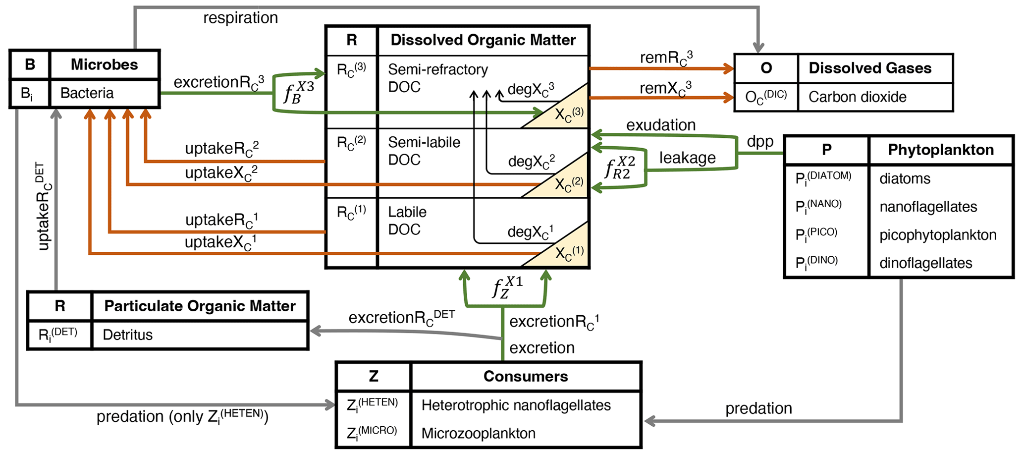
Figure 1Schematic representation of the hypothesized interactions regulating the concentrations of CDOM and DOC in the surface layers of the open waters of the NW Mediterranean Sea. The boxes show the BFM state variables, and the yellow triangles show the three state variables that represent three reactivities of CDOM. Green arrows indicate fluxes of DOC and CDOM production (excretion, excretion, exudation and leakage; mg C m−3 d−1), orange arrows indicate fluxes of DOC and/or CDOM degradation through direct bacterial consumption (uptake, uptake, uptake, uptake; mg C m−3 d−1) or indirect remineralization (rem, rem; mg C m−3 d−1), and black arrows indicate photobleaching processes (deg, deg, deg; mg C m−3 d−1). The names in italics (, , and ; dimensionless) represent the fractions that divide the flux between CDOM and non-coloured DOC. The subscript i appended to each living component and detritus indicates the elemental constituents among carbon (C), nitrogen (N), and phosphorus (P), with Chl a only being used for phytoplankton and silica (Si) only being used for diatoms.
Bio-optical properties of CDOM, detritus, and phytoplankton
The optical constituents of the spectrally resolved version of BFM are the four PFTs, detrital particles, and the three forms of CDOM corresponding to their resistance to bacterial metabolic activity. CDOM absorbs light and has a negligible contribution to scattering; therefore, CDOM absorption at 450 nm, aCDOM(450) (m−1), is first calculated as the product of CDOM biomass (, mg C m−3) and the mass-specific absorption coefficients at 450 nm (, m2 mg C−1). CDOM absorption as a function of wavelength (λ), aCDOM(λ) is modelled with an exponential function, decreasing with increasing λ:
where is the spectral slope of the CDOM absorption coefficients between 350 and 500 nm.
Detritus absorbs and scatters light. Detritus absorption at 440 nm (aNAP(440), m−1) is calculated as the product of the carbon component of detritus (, mg C m−3) and their mass-specific absorption coefficients at 440 nm (, m2 mg C−1), and then the absorption spectrum of detritus is modelled as an exponential function which decreases with increasing λ:
where is the spectral slope of the detritus absorption coefficients, which we have set to 0.013 nm−1 (Table 1). Detrital scattering at 550 nm (bNAP(550), m−1) is calculated as the product of and the mass-specific scattering coefficient at 550 nm (, m2 m C−1), and then the scattering spectrum of detritus, bNAP(λ), is computed as an exponential function of λ:
where eR is an exponent set to 0.5 (Table 1).
To describe the optical properties of phytoplankton, we used Chl a-specific absorption spectra ( of different phytoplankton taxa growing in culture under different light, nutrient supply, and temperature conditions. We considered 177 spectra, digitized from the literature and provided as supplementary material in Álvarez et al. (2022). Each was decomposed into the contribution of Chl a; photosynthetic carotenoids; photoprotective carotenoids (PPCs); and a fourth pigment group that was made up of phycoerythrin for Synechococcus species, Chl b for green algae taxa and Prochlorococcus species, and Chl c for the other taxa. To obtain the relative pigment concentrations for each pigment group we fitted a multiple-linear-regression model to the weight-specific absorption spectra for each pigment group obtained from Bidigare et al. (1990) in order to obtain the lowest sum of residuals between the predicted and the measured (Hickman et al., 2010). The Chl a-specific absorption spectra for photosynthetic pigments only ( were reconstructed using the obtained relative concentrations excluding PPCs (Babin et al., 1996). From this collection of spectra, and were averaged for picophytoplankton, nanophytoplankton, diatoms, and dinophyta taxa. The resulting four were used to calculate the total absorption by phytoplankton (aPH(λ), m−1) as the sum of the products of PFT Chl a (, mg Chl a m−3) and the Chl a-specific absorption coefficients (m2 mg Chl a−1):
Scattering coefficients of phytoplankton were assumed to be functions of phytoplankton biomass (, mg C m−3) and the C-specific spectra taken from Dutkiewicz et al. (2015). Scattering coefficients by all phytoplankton (bPH(λ), m−1) were calculated as the sum of the product of phytoplankton biomass and the C-specific scattering spectrum for each of the four PFTs (m2 mg C−1):
The phytoplankton absorption cross-sections for all pigments (, m2 mg Chl a−1), photosynthetic pigments (, m2 mg Chl a−1), and the scattering cross-section (, m2 mg Chl a−1) were computed as the average of , , and between 387.5 and 800 nm, respectively. These aggregated values were used to perturb the magnitude of their respective spectra without modifying the spectral shape. The computation of and is equivalent to Eq. (19), substituting with and , respectively:
Total absorption, scattering, and backscattering (a(λ), b(λ), and bb(λ), respectively) depend on the additive contribution of seawater and the BGC constituents along the water column. Total a(λ) (m−1) is calculated from the absorption by water (aW(λ), m−1, Pope and Fry (1997)), CDOM, detritus, and phytoplankton:
Total b(λ) (m−1) is calculated as the sum of the scattering of water (bW(λ), m−1, Smith and Baker (1981)), detritus, and phytoplankton:
Total bb(λ) (m−1) is computed as the sum of each constituent's scattering multiplied by constant and λ-independent backscattering-to-scattering ratios (bbrW, bbrR, and that were 0.5 for water (Morel, 1974), 0.005 for detritus (Gallegos et al., 2011), 0.002 for P(DIATOM) (Dutkiewicz et al., 2015), 0.0071 for P(NANO) (Gregg and Rousseaux, 2017), 0.0039 for P(PICO) (Gregg and Rousseaux, 2017; Dutkiewicz et al., 2015), and 0.003 for P(DINO) (Dutkiewicz et al., 2015) (Table 1):
Spectrally resolved light transmission and computation of E0(λ,z)
Incoming spectral irradiance at the top of the ocean was obtained from the OASIM model interfaced with the European Centre for Medium-Range Weather Forecast (ECMWF) atmospheric model (Lazzari et al., 2021a). Input data contained two downward streams just below the surface of the ocean: direct [Ed(λ, 0−)] and diffuse [] (both in W m−2 and averaged at 33 wavebands). Irradiance along the depth of the water column (z) was described with three state variables (all in W m−2): downwelling direct [Ed(λ,z)] and diffuse [Es(λ,z)] components and an upward diffuse component [Eu(λ,z)]. The vertically resolved three-stream propagation was resolved with the following system of differential equations (Aas, 1987; Ackleson et al., 1994; Gregg, 2002):
where a(λ,z) is the total absorption (Eq. 20), b(λ,z) is the total scattering (Eq. 21), and bb(λ,z) is the total backward scattering (Eq. 22) at depth z (all in m−1). rs, ru and rd are the effective scattering coefficients, and υd, υs, and υu are the average cosines of the three streams, which are constant for diffuse radiance but vary with solar zenith angle for direct radiance. For details on the derivation of the solution, see Terzić et al. (2021).
At the centre of the depth layer, Ed(λ,z), Es(λ,z), and Eu(λ,z) were averaged between the top and the bottom of the layer, and total scalar irradiance, E0(λ,z), was computed by scaling the three streams by their inverse average direction cosines. E0(λ,z) was converted from irradiance values (in units of W m−2) to photon flux (given in µmol quanta m−2 d−1) by multiplying by λ in metres, dividing by the product of the Avogadro's constant (NA), Planck's constant (h), and speed of light (c) and converting mol quanta to µMol quanta and seconds to days:
E0(λ,z) was the light available for phytoplankton growth (Eq. 2) at depth z, and its integral value from 387.5 and 800 nm constituted the photosynthetically available radiation (PAR) that was used as the light input for CDOM photobleaching (Sect. 2.1.2.1, Eq. 13).
2.2 Observations
The Mediterranean Sea is a semi-enclosed marginal sea. The Ligurian Sea, in the NW Mediterranean Sea, is characterized by oligotrophic to moderately eutrophic waters. The BOUSSOLE and the DYFAMED (Dynamique des Flux Atmosphériques en Méditerranée) monitoring sites, both in the Ligurian Sea, provided bio-optical and physical–chemical measurements, respectively (Sect. 2.2.1). In addition, we considered ocean-colour data collected by satellites (Sect. 2.2.2) (Fig. 2).
2.2.1 In situ data at BOUSSOLE and DYFAMED sites
The BOUSSOLE project includes a permanent optical mooring deployed at 43∘22′ N, 7∘54′ E, where the depth is 2440 m, collecting optical data at a high temporal resolution, and oceanographic cruises that visit the site monthly to collect optical and BGC variables (Golbol et al., 2000). Only data from monthly cruises were used in the present work. Seawater is generally collected at 12 discrete depths within the 0–400 m water column (5, 10, 20, 30, 40, 50, 60, 70, 80, 150, 200, 400 m). Sampling is performed with a SeaBird SBE911+ CTD/rosette system equipped with pressure (Digiquartz Paroscientific), temperature (SBE3+), and conductivity (SBE4) sensors and 12 L Niskin bottles, from which water samples are collected for subsequent absorption measurements and high-performance liquid chromatography (HPLC) analyses. The CDOM absorption measurements are described in Organelli et al. (2014) and references therein. We only remind here that the spectral slope of aCDOM(λ) was determined between 350 and 500 nm (, although shorter UV λ intervals have also been used to report spectral slopes in the Mediterranean Sea (275–295 nm, Catalá et al., 2018). Particulate light absorption spectra, aP(λ), were measured using the quantitative filter pad technique (QFT) (Mitchell, 1990; Mitchell et al., 2000), and the protocol is described in Antoine et al. (2006). aP(λ) was decomposed into phytoplankton and detrital absorption coefficients, aPH(λ) and aNAP(λ), respectively, using the numerical decomposition technique of Bricaud and Stramski (1990). The HPLC procedure used to measure phytoplankton pigment concentrations is fully described in Ras et al. (2008). The fractions of picophytoplankton, nanophytoplankton, and microphytoplankton were calculated following the diagnostic pigments method (Uitz et al., 2006).
The Dynamique des Flux Atmosphériques en Méditerranée (DYFAMED) time series station (Marty, 2002) is located at 43.25∘ N and 7.54∘ E, where data have been collected since 1991. Temperature (T) and salinity (S) data were collected within the 0–2400 m water column with the same CTD/rosette configuration used at BOUSSOLE with nutrients sampled at discrete depths. T and S data from 1994 to 2014 were downloaded from the OceanSITES Global Data Assembly Centre, and nitrate, nitrite, and phosphate concentrations were downloaded from Coppola et al. (2021).
2.2.2 Data from satellites
Satellite-retrieved IOPs and Chl a were obtained from the OCEANCOLOUR_MED_BGC_L3_MY_009_143 product (EU Copernicus Marine Service Information, 2022). The product provides multi-sensor RRS(λ) spectra (SeaWiFS, MODIS-AQUA, NOAA20-VIIRS, NPP-VIIRS, and Sentinel3A-OLCI) merged using the state-of-the-art multi-sensor merging algorithms and shifted to the standard SeaWiFS wavelengths (412, 443, 490, 555, and 670 nm). IOPs (aPH(443) and aDG(443)) are derived from RRS(λ) via the Quasi-Analytical Algorithm version 6 (QAAv6) model (Lee et al., 2002). Chl a concentration is determined using the Mediterranean regional algorithm, an updated version of MedOC4 (Volpe et al., 2019) and AD4 (Berthon and Zibordi, 2004), merged according to the water type present (Mélin and Vantrepotte, 2015; Volpe et al., 2019). For all variables, to obtain the time series from January 2011 to December 2014 at the study site, we extracted a 20×20 km box around the BOUSSOLE site (from 43.27 to 43.47∘ N in latitude and from 7.77 to 8.03∘ E in longitude) and averaged it when available observations covered at least 20 % of the area.
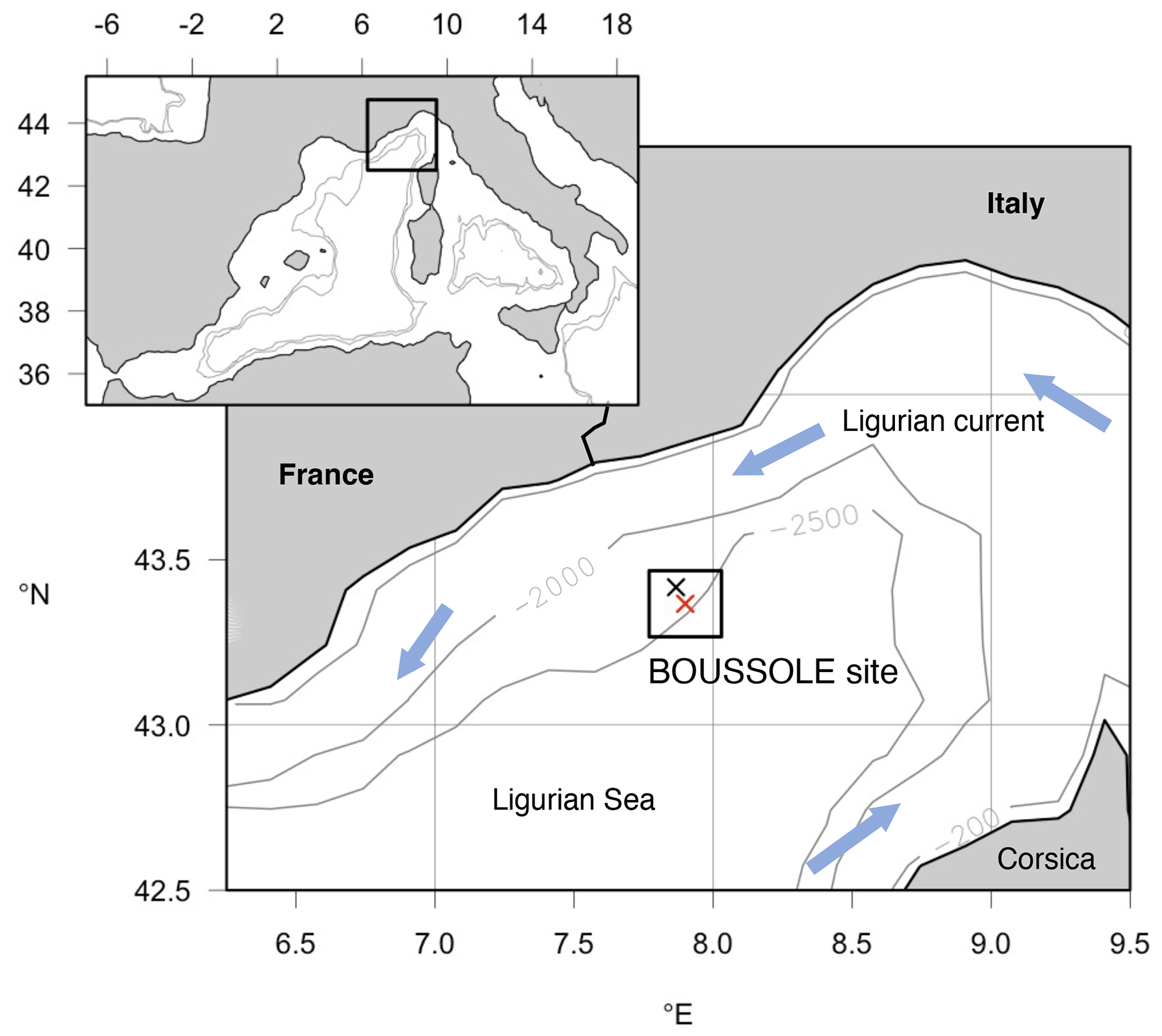
Figure 2Map showing the location of the BOUSSOLE mooring site (red cross) and the DYFAMED site (black cross) in the Ligurian Sea (NW Mediterranean Sea). The box surrounding the sites indicates the 20×20 km area considered for averaging data from the daily 1 km Copernicus Marine Service product to obtain the time series of satellite data at the study site.
2.3 Study region and setup of the 1D model for the BOUSSOLE site
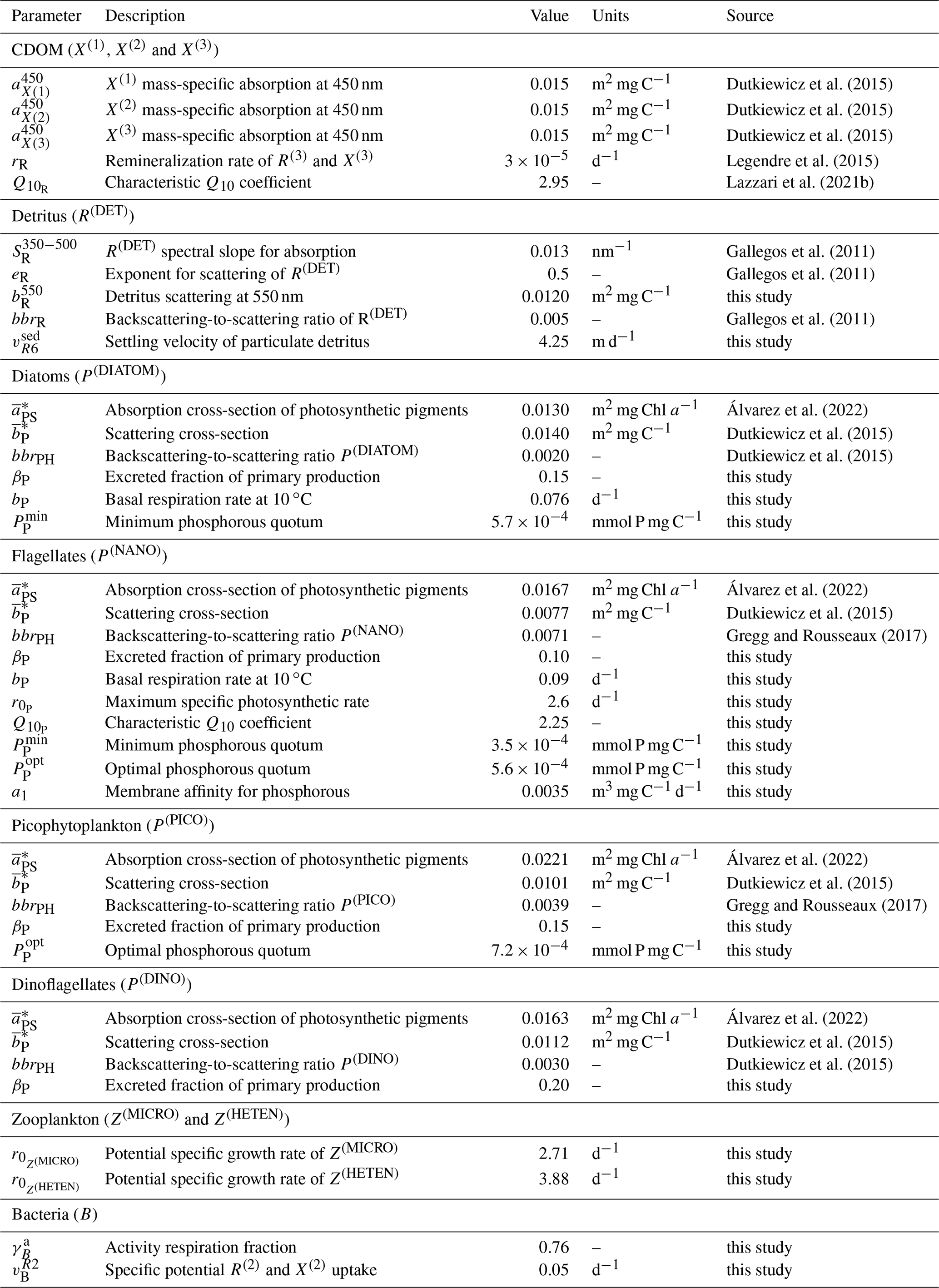
The configuration of the one-dimensional spectrally resolved version of the BFM used to simulate the BOUSSOLE site has the same parameter values as the 3D configuration of the BFM for the Mediterranean Sea, except for those reported in Table 1. Some updates comprised parameters related to the growth of nanophytoplankton (P(NANO)), in particular those related to the uptake of phosphorous (a1, , and . This update was set to reproducing the high contribution of nanophytoplankton to the total Chl a content at the BOUSSOLE site (Antoine et al., 2006) (see Fig. 4). We also updated the parameters for the production by phytoplankton and the consumption by bacteria of semi-labile DOC (βP and to simulate accurately the seasonality of DOC concentrations in the superficial waters of the site (Avril, 2002) (see Fig. 5). The parameter values related to the partition between dissolved and particulate excretion in Z(MICRO) and Z(HETEN) and the mortality of Z(CARNI) and Z(OMNI) are equal to the up-to-date values in Álvarez et al. (2022) together with all the optical parameters. All the other parameter values are equal to those shown in Lazzari et al. (2012).
The 1D configuration of GOTM-(FABM)-BFM for the BOUSSOLE site consists of (i) a water column of 2448 m subdivided into 196 vertical levels with a higher resolution at the surface and bottom, which were generated using the iGOTM web tool (https://igotm.bolding-bruggeman.com/, last access: 12 October 2021); (ii) atmospheric forcing that included hourly 10 m winds, 2 m air temperature and humidity, sea level pressure, precipitation, and cloud cover from ECMWF ERA5; atmospheric pCO2 that was set to a constant value of 400 ppm; and spectral plane downwelling irradiance at 15 min frequency from the OASIM model that has been validated for the BOUSSOLE site (Lazzari et al., 2021a); and (iii) initial conditions for T, S, and BGC variables.
Observed vertical profiles of T and S at the DYFAMED site from 2009 to 2014 were edited to match the GOTM profile format and were used as initial conditions and constrained by a monthly nudging in order to reproduce the intensity and timing of the mixing as closely as possible to observations. Monthly vertical profiles of BGC variables (nitrate, phosphate, silicate, O2, DIC, and alkalinity) were obtained from the Copernicus reanalysis (Cossarini et al., 2021), linearly interpolated onto the model vertical grid, and used for initialization and constrained by a yearly nudging. All other variables were set to constant values throughout the water column. The initial values of , , and were 80, 400, and 480 mg C m−3, respectively, consistent with DOC concentrations at depth in the western Mediterranean Sea (Catalá et al., 2018; Santinelli, 2015; Galletti et al., 2019). The initial values of , , and were 1, 3, and 1.25 mg C m−3, respectively. Given that below 200 m depth the BFM simulates negligible concentrations of and , the initial concentration of was chosen to match aCDOM(450) values observed at the site below 100 m (Organelli et al., 2014) and aCDOM(250) and aCDOM(325) values observed in the western Mediterranean Sea below 200 m (Catalá et al., 2018). All PFTs were initialized to 8 mg C m−3 and 0.16 mg Chl a m−3. Bacteria and zooplankton were initialized to 1 mg C m−3.
A 6-year hindcast (January 2009 to December 2014) was conducted, covering the period for which all the necessary forcing data were available. The first 2 years were considered as model spin-up, and the next 4 years were considered for the optimization. The source for the setup can be found in the “Code availability” section.
Table 1Values of the BFM optical and BGC parameters that were not optimized. The parameters with the source “this study” were manually chosen in order to obtain a good approximation of model results to findings by Avril (2002) and Antoine et al. (2006) with regard to the concentration of DOC at DYFAMED and PFT Chl a at BOUSSOLE, respectively.
2.4 Optimization strategy and simulations for hypothesis testing
The final step in completing the GOTM-(FABM)-BFM configuration at the BOUSSOLE site was to integrate the model and observations to drive the simulated output as closely as possible to the observations. Being computationally light, the one-dimensional BFM configuration has the advantage of allowing many simulations in a reasonable time, which provided us with a powerful tool for optimizing a relatively large number of parameters (Sect. 2.4.1) through a genetic algorithm that minimizes the misfit between the model and the observations (Sect. 2.4.2) and for investigating processes based on the proposed new parameterizations (Sect. 2.4.3).
2.4.1 Parameters optimized
Observations used for optimization were all collected at the BOUSSOLE site at a monthly temporal resolution and roughly at the same number of discrete depths and included pico-, nano-, and micro-phytoplankton Chl a (pico Chl a, nano Chl a, and micro Chl a, respectively); aPH(450); aNAP(450); aCDOM(450); and . The potential number of independent parameters included in the optimization problem is limited by the observations available and by the fact that optimized parameters must appear in some process independently. A total of 25 optical and BGC parameters were optimized (Table A1 in Appendix A), and all of them were given a positive range of values for initialization and evolution without conditions or trade-offs for the consistency between pairs of parameters. The rest of the parameters not included in the optimization kept constant values (Table 1). The only observations related to CDOM were aCDOM(λ), which depend on both the mass concentration and the mass-specific absorption coefficients across the electromagnetic spectrum. We assumed the absorption coefficients of the three reactivities to be constant at 450 nm (, , and , and we optimized parameters related to the production of CDOM (, , , , , , and and those related to the photobleaching of (bX(3) and IX(3)). The spectral slope of the CDOM pool has been associated with aromaticity and the average molecular weight of the CDOM compounds (Blough and Green, 1995) but appears to be less linked to CDOM concentration. Therefore, the spectral slopes between 350 and 500 nm for the three reactivities (, , and were optimized to ensure the proper simulation of aCDOM(λ) in wavebands other than 450 nm. For phytoplankton, independent observations regarding mass concentrations (Chl a) and optical properties (aPH(λ)) were available; therefore, both types of parameters were optimized. We optimized the absorption cross-sections ( and the maximum Chl a : C quota ( as they appear independently in light attenuation (Eq. 17) and in photoacclimation (Eq. 19 in Álvarez et al., 2022) and in CDOM production (Eq. 5), respectively. The absorption cross-sections of photosynthetic pigments ( and the photochemical efficiencies ( of the PFTs appear only in photosynthesis (Eq. 2). We opted to optimize only one of these two interdependent parameters and therefore kept constant and optimized . The choice responds to the fact that can be inferred from the observed aPH(λ) of multiple phytoplankton taxa, and , instead, is not well documented in the literature, being more difficult to measure. For detritus, we optimized the reference absorption coefficients at 440 nm ( and kept constant all the BGC parameters that alter the mass concentrations. Given that aNAP(λ) observations were available, optical parameters related to the spectral shape of absorption by detritus ( could have been included in the optimization, but we decided to maintain this parameter as constant given the small contribution of aNAP(λ) to the total non-water absorption as compared to CDOM and phytoplankton. All parameters related to scattering and backscattering of both phytoplankton ( and bbrPH) and detritus (, eR, and bbrR) were not included in the optimization.
2.4.2 Parameter optimization method
To perform the estimation of model parameter values using observational data, we used the Parallel Sensitivity Analysis and Calibration utility (ParSAC, Bruggeman and Bolding, 2020). ParSAC applies the Differential Evolution (DE) algorithm (Storn and Price, 1997), which is inspired by the rules of natural selection. Different individuals have different fitness values in terms of how well they simulate observations. A higher fitness value indicates a combination of parameters that reproduce better observations and therefore must persist in the next generation. ParSAC formulates such a fitness (i.e. the probability that the candidate parameter values are the true parameter set representing reality) as a multi-objective function calculated as the log-transformed likelihood between the outcome of the model and the observations provided, assuming the observed values are log-normally distributed, with the median being equal to the model prediction. For any variable observed from a total number of M observed variables, there will be Nm number of pairs consisting of observations On and corresponding simulation-based estimates Pn (model results at the temporal and spatial observation locations). The sum of squares of the residuals for each variable observed m (SSQm) is computed as follows:
For M variables observed, all differences between the model and observations are combined as follows:
Each individual in a given population of size S=288 is a 25-dimensional target vector that represents a candidate solution to the problem. The parameter values in the target vectors in the first generation are sampled uniformly between minimum and maximum values, which are listed in Table A1 (Appendix A). The DE algorithm creates new generations of individuals by applying cycles of mutation, crossover, and selection operating on the target vectors. Mutation means that, once all simulations in a generation are completed, the DE algorithm creates a new set of S mutant vectors. In this implementation, each mutant vector is created by randomly selecting three targets (xr1, xr2, and xr3) and applying a mutation operator that consists of . Crossover means to increase the diversity of the parameter vectors; crossover is done to generate the final trial set of individuals. Here, crossover is performed between each target vector and its corresponding mutant vector, retaining each element of the target vector in the population with a probability of 0.9, otherwise introducing the corresponding element from the mutant vector. Selection, which is the final phase, is where the lnLikelihood of the trial vector is compared to the lnLikelihood of the corresponding target vector. The trial vector replaces the target if the lnLikelihood value obtained from the trial is higher than or equal to the lnLikelihood obtained from the target vector. After the selection procedure, the size of the population is again S. The cycle of mutation, crossover, and selection is carried out iteratively, and eventually, the DE algorithm provides an estimate of the optimal parameter values that minimizes the misfit between the model output and the observations (i.e. maximizes the sum of likelihoods in the population). Genetic algorithms are particularly robust in overcoming local minima (Storn and Price, 1997). As a parallel search technique that runs several vectors simultaneously, superior parameter configurations can help other vectors escape local minima and therefore avoid misconvergence. After passing through each generation, ParSAC checks whether the end condition is met, which, in this work, was a maximum number of 180 generations, after which the range of lnLikelihoods in the population was less than 0.005. The optimal solution for the 25 parameter values was extracted as the mean of the parameter distribution in generation 180. To determine the success achieved through optimization, we calculated the correlation coefficient (R) and the root mean squared error (RMSE) for each observation compared to the model output for each generation.
2.4.3 Simulations and hypothesis-testing experiments
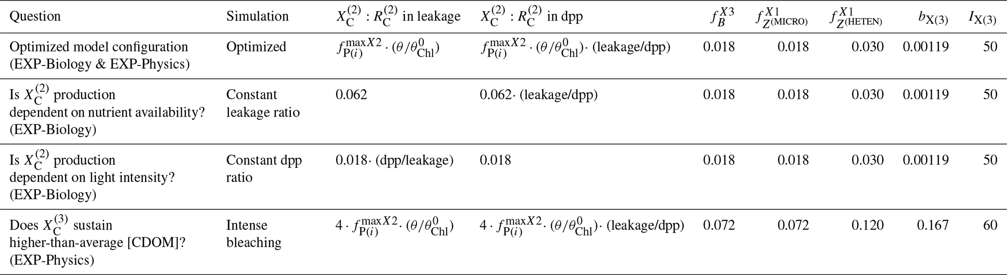
The model configuration described in Sect. 2.3 and the optimized parameter values obtained as described in Sect. 2.4.2 represent the optimized model configuration. We used a series of hypothesis-testing experiments to investigate the mechanisms that determine the vertical and temporal patterns of CDOM distribution at the BOUSSOLE site. Those experiments consisted of three more simulations in which we changed some of the assumptions of the optimized configuration. All simulations are summarized in Table 2, all were run for 6 years with 2 years of spin-up, and the results were analysed for the last 4 years (January 2011 to December 2014).
In the first experiment, EXP-Biology, we investigated the role of nutrient and light limitations in controlling the biogenic in situ production of biodegradable CDOM and therefore in generating the observed aCDOM(λ) values. This experiment consisted of comparing the results of the optimized configuration with two additional simulations. These additional simulations are (1) the constant leakage ratio, in which we considered the proportion : in phytoplankton dpp to be a constant fraction of leakage and therefore removed the dependence of on , and (2) the constant dpp ratio, in which we considered the fraction : in dpp to be constant and therefore removed the dependencies of on and on leakage/dpp.
In the second experiment, EXP-Physics, we investigated the role of allochthonous CDOM in maintaining CDOM concentrations in the surface ocean. This experiment consisted of comparing the results of the optimized configuration with an additional simulation of intense bleaching, in which we prescribed the same photobleaching parameters for (bX(3) and IX(3)) as we did for the other two CDOM pools and quadrupled the CDOM : DOC fractions in all biotic sources (, , , , , , and . By comparing the optimized configuration with the intense-bleaching simulation, we evaluated whether an increased, locally produced CDOM could compensate for a reduced allochthonous input and the extent to which the optimized simulation was able to represent the role of , and thus of any source of allochthonous CDOM, in generating the observed aCDOM(λ) values.
Table 2List of simulations performed to test the findings provided by the optimized framework. The list reports all the formulations and/or parameter values which distinguish the test simulations from the optimized model configuration.
3.1 Skill of the optimized simulation
In this section we evaluate how the optimized model configuration reproduces seasonal cycles and vertical gradients in terms of biological and optical variables. We compared the output of the optimized simulation with in situ observed data of mixing and nutrients (Sect. 3.1.1), BGC variables (Sect. 3.1.2), and IOPs (Sect. 3.1.3) and with satellite-retrieved data not used in the optimization (Sect. 3.1.4). The optimized parameter values and the quantitative model data skill metrics (R and RMSE) achieved throughout optimization can be found in Appendix A.
3.1.1 Mixing and nutrients
The temporal evolution of a climatological year (2011–2014) of the temperature in the water column is presented for the observations (Fig. 3a) and for the optimized model run (Fig. 3b). Overall, there is good agreement in terms of both the timing of the stratification and the mixing events. The seasonal cycles of nitrate (Fig. 3c vs. 3d) and phosphate (Fig. 3e vs. 3f) are well captured, along with the depth of the nitracline, which ranges from 45 m at the onset of the stratification to 60 m at the end of the year, with NO3 and PO4 being underestimated by approximately 25 % in the deeper layer.
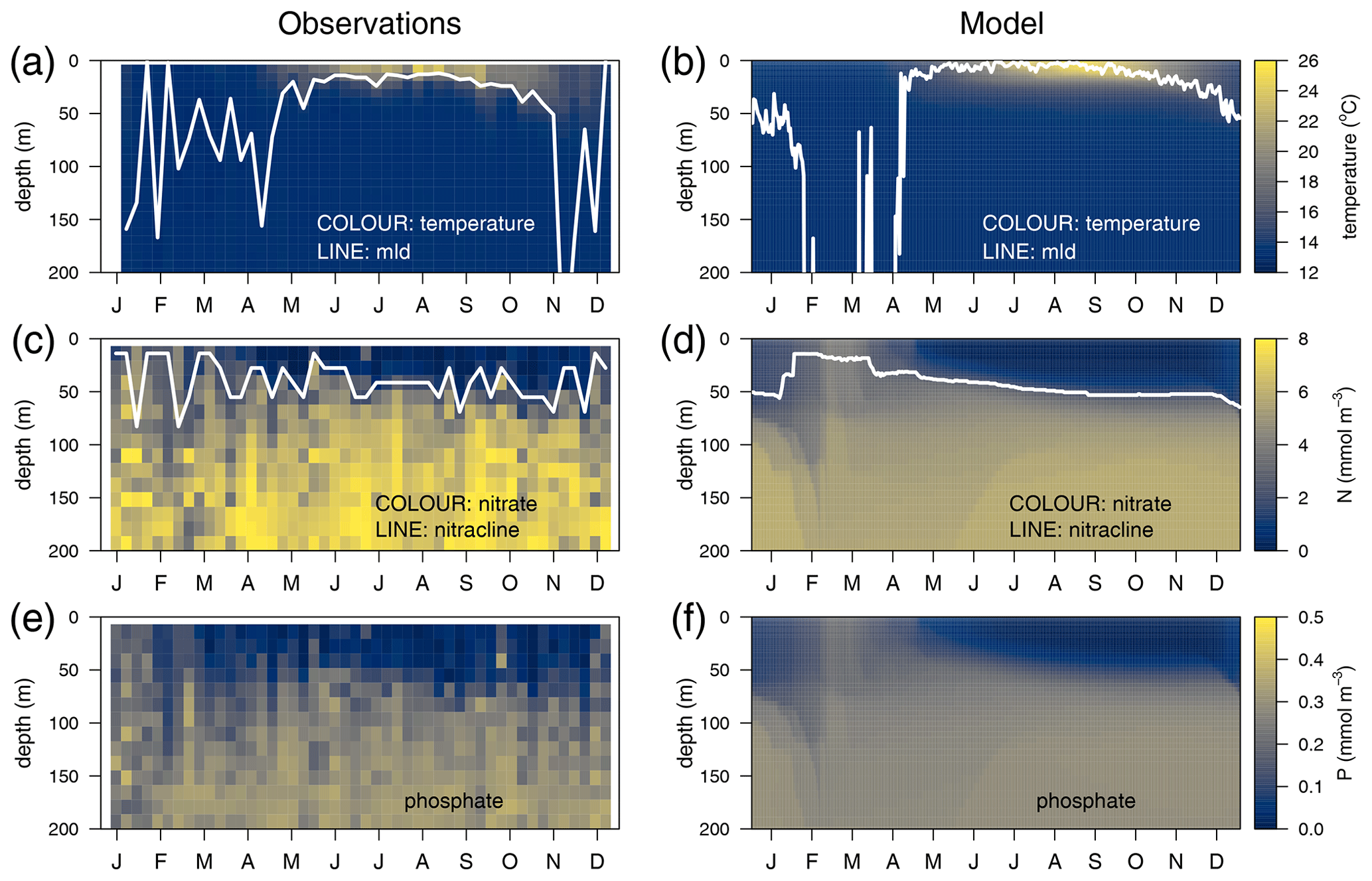
Figure 3Annually averaged vertical profiles as a function of time of (a–b) temperature, (c–d) nitrate, and (e–f) phosphate, obtained from observations at the DYFAMED site (a, c, e) and from the optimized simulation (b, d, f). The white line in the temperature panels represents the mixed-layer depth (mld) obtained in (a) with a threshold of 0.2 ∘C for temperature (de Boyer Montégut et al., 2004) and in (b) with a threshold of m2 s−2 for turbulent kinetic energy. The line in (c) and (d) represents the nitracline (nitrate concentration equals 2 µM).
3.1.2 Chl a, DOC, and CDOM
Observations show maximum Chl a concentrations of more than 1 mg m−3 in the first 30 m of the water column in March–April and the formation of a DCM in April–May that deepens down to around 50 m and gradually shoals after October (Fig. 4a). The model succeeds in capturing the important spatial features of the site's mean total Chl a (TChl a) field, such as the formation of a DCM in April–May that reaches 50 m depth in September–October (Fig. 4e). However, the simulated maximum Chl a concentrations are about 45 % smaller than the observations (Fig. 4e vs. 4a), and, therefore, the optimized simulation generally underestimates the vertically integrated Chl a. The subdivision of Chl a into size fractions follows the main features observed at BOUSSOLE, which include a larger contribution of phytoplankton larger than 2 µm to the superficial bloom in March–April (Fig. 4g and h) and the noticeable contribution of nanophytoplankton to the TChl a at the site (Antoine et al., 2006) (Fig. 4c).
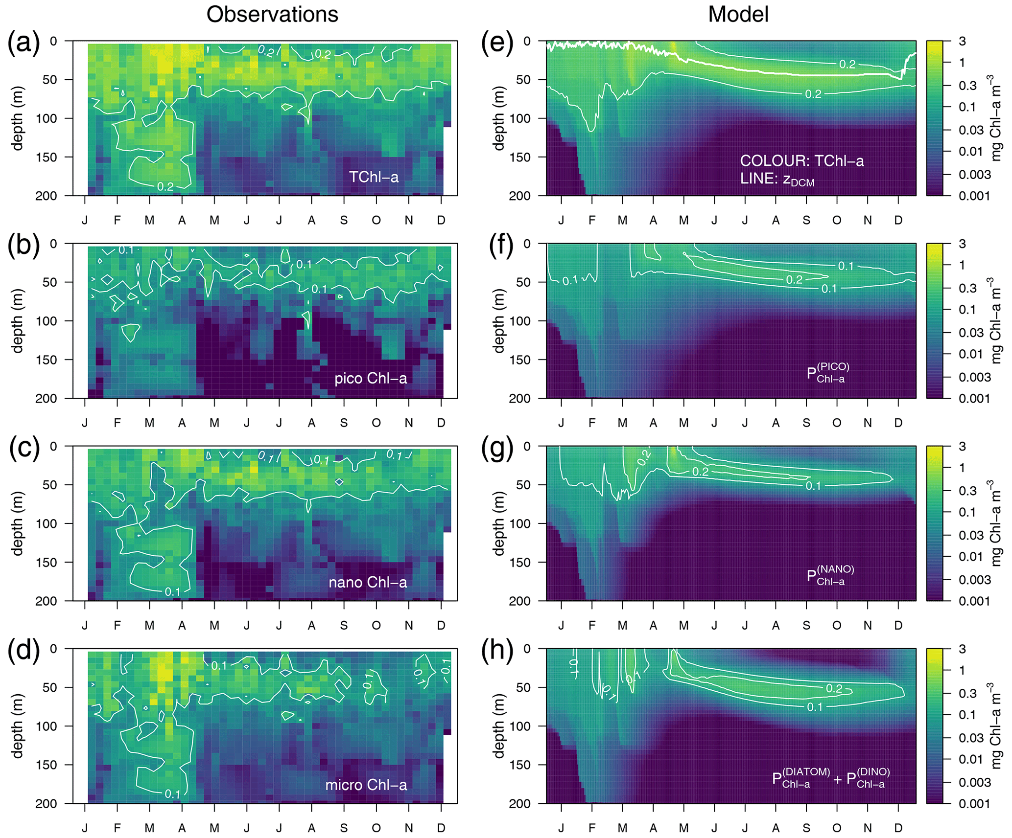
Figure 4Annually averaged vertical profiles as a function of time of log-transformed total Chl a – (a) and (e), picophytoplankton Chl a – (b) and (f), nanophytoplankton Chl a – (c) and (g), and microphytoplankton Chl a – (d) and (h) obtained from observations at the BOUSSOLE site (left panels) and from the optimized simulation (right panels). The thick line in (e) represents the depth of the DCM.
Simulated DOC and CDOM showed clear and very different seasonal dynamics (Fig. 5). After a period of winter mixing, when the concentrations of both variables were homogeneously distributed in the column, with DOC values between 38–40 µM (Fig. 5a) and CDOM concentrations at about 1.2 mg C m−3(Fig. 5b), superficial concentrations of both variables started to increase in March. While CDOM concentrations reached a maximum in May and decreased rapidly at the surface afterwards, DOC concentration had a maximum in June and gradually decreased until the following winter. CDOM formed a sub-superficial maximum in May–June that deepened down to 50 m in October–November; this feature was absent in DOC.
3.1.3 Inherent optical properties (IOPs)
The optimized model configuration captured important features of the mean site aPH(450) field, which mainly follows the distribution of TChl a (Fig. 6a). After the general vertical homogeneity established in winter, the maximum values (0.05 m−1) are found at the surface in spring; in summer, the maximum is located around 40–50 m, and the lowest values (0.005 m−1) are found at the surface and below 75 m (Fig. 6b). Observed aNAP(450) showed very low values (0.01 m−1) (Fig. 6c) comparable to those simulated (Fig. 6d). Observed aCDOM(450) showed clear seasonal dynamics with rather vertically homogeneous values (0.018–0.02 m−1) until April and a subsurface maximum from April to September at 30–50 m depth. After September, aCDOM(450) tended to be more homogeneous from the surface to 130 m while still being relatively high compared to winter (Fig. 6e). In the optimized simulation, aCDOM(450) follows the distribution found for the observations and was therefore homogeneously distributed during winter (0.02 m−1) and increased to values up to 0.04 m−1 at the surface in April. Thereafter, the maximum values were confined to the depth of the yellow-substance maximum (YSM) formed at 30 m depth in June and deepened throughout summer down to 50 m in December (Fig. 6f). Our depth profile data showed that the simulated depth of the YSM (Fig. 6f) was only slightly shallower than that of the DCM (Fig. 6e), which is consistent with reports from Oubelkheir et al. (2007) and Xing et al. (2014) in the NW Mediterranean Sea.
3.1.4 Validation with satellite products
Satellite-retrieved Chl a, aPH(443), and aDG(443) from January 2011 to December 2014 at the BOUSSOLE site are compared with simulated values, averaged over the first optical depth of the water column (Fig. 7). In the 4-year time series considered, the simulated first optical depth ranged from 4.8 to 28 m. The simulated Chl a values are slightly underestimated with respect to the satellite value (bias of −0.028 mg m−3), especially in the period from June to October. If the mixing periods in February and March, when simulated TChl a concentrations drop to almost zero, are excluded from the comparison, Pearson's correlation coefficient is 0.55. The simulated aPH(450), on the other hand, has a correlation coefficient with aPH(443) of 0.69 with no bias, suggesting that the optimized values of compensated for the underestimation of Chl a. Simulated aDG(450) has a correlation coefficient with aDG(443) of 0.40 with some degree of underestimation (bias of −0.0031 m−1). The optimized simulation could not capture increments in aDG(443) during November–December, probably because these maxima were not recorded by the BOUSSOLE in situ measurements at a monthly resolution.
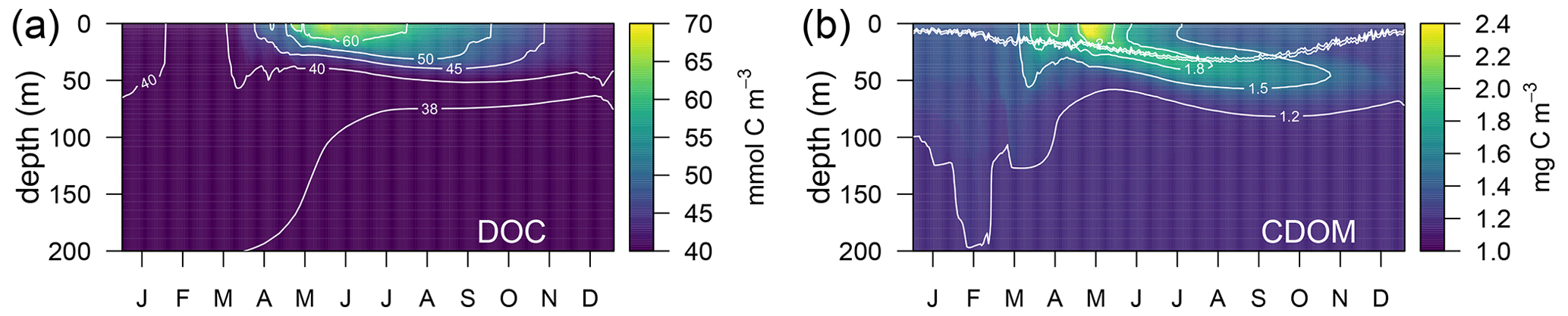
Figure 5Annually averaged vertical profiles as a function of time of (a) total dissolved organic carbon (DOC) and (b) total CDOM in the optimized simulation. The double line in (b) shows the position of the 50 and 60 µmol quanta m−2 s−1 of PAR that represent the PAR threshold for maximum bleaching of the biodegradable (bX(1) and bX(2)) and the semi-refractory CDOM (bX(3)), respectively.
3.2 Dynamics of CDOM in relation to other BGC products
In this section, we analyse the results of the optimized simulation to investigate the following: (i) the vertical and seasonal dynamics of aCDOM(λ) in relation to phytoplankton, bacteria, and DOC (Sect. 3.2.1); (ii) the mutual proportions of CDOM, phytoplankton, and detritus in the absorption budget (Sect. 3.2.2); and (iii) the ability to reproduce observed bio-optical relationships between aCDOM(λ) and other BGC variables (Sect. 3.2.3).
3.2.1 Seasonal and vertical dynamics of aCDOM(450)
The average 4-year depth profiles of TChl a, aCDOM(450), bacterial carbon (BC), and dissolved organic carbon (DOC) simulated for the BOUSSOLE site (depth <200 m) and their seasonal patterns are shown in Figs. 8 and 9. During winter (January to March), when deep convective water mixing occurred, TChl a was high (0.2–0.3 mg m3) and homogeneously distributed within the 0–75 m layer, while it rapidly decreased to values close to 0.02 mg m−3 below 80 m. DOC and aCDOM(450) show vertical homogeneity in winter, with values around 40 µM and 0.02 m−1, respectively (Fig. 8, winter). A sub-superficial maximum of TChl a formed in spring between 30–40 m, a aCDOM(450) maximum formed at 30 m depth, whereas the maximum values of DOC and BC remained within the first 10 m. There, DOC reached the highest seasonal concentration, with 66 µM (Fig. 8, spring). The sub-superficial maximum of TChl a deepened in summer to 45 m. A reduction of surface aCDOM(450) values was observed from spring to summer, and the subsurface maximum was reinforced and deepened to 40 m. A BC subsurface maximum was also formed slightly above the aCDOM(450) maximum and at least 10 m above the DCM (Fig. 8, summer). Chl a-depleted surface waters and a weaker DCM persisted in fall. A maximum of aCDOM(450) was also observed in fall but in slightly deeper waters, closer to the DCM (Fig. 8 Fall).
In terms of temporal dynamics, TChl a reached maximum concentrations (0.7 mg m−3) at the end of winter and gradually decreased to values of 0.05 mg m−3 in summer because of the depletion of nutrients due to the strong stratification of the water column (Fig. 9a). At the same time, a DCM formed at approximately 40 m depth, and its TChl a content increased throughout summer (Fig. 9b). The increase of aCDOM(450) started at the same time as the TChl a increase but persisted much longer, when TChl a was much lower and BC remained high (Fig. 9a). In the DCM, the maximum aCDOM(450) values were at a similar level of maxima from March to June (Fig. 9b). While in the DCM, aCDOM(450) and DOC followed the same temporal pattern (Fig. 9b), at the surface, the maximum of aCDOM(450) was reached 2 months earlier than that of the DOC, which continues to accumulate during most of the spring, whereas aCDOM(450) decreases as a result of photobleaching (Fig. 9a). The similar temporal patterns of aCDOM(450) and BC at the surface (Fig. 9a) and especially at the DCM (Fig. 9b) indicate a possible involvement of bacteria in CDOM production, although in our optimized simulation, semi-refractory CDOM is mainly of allochthonous origin (see Sect. 3.3.2 for a more detailed analysis).
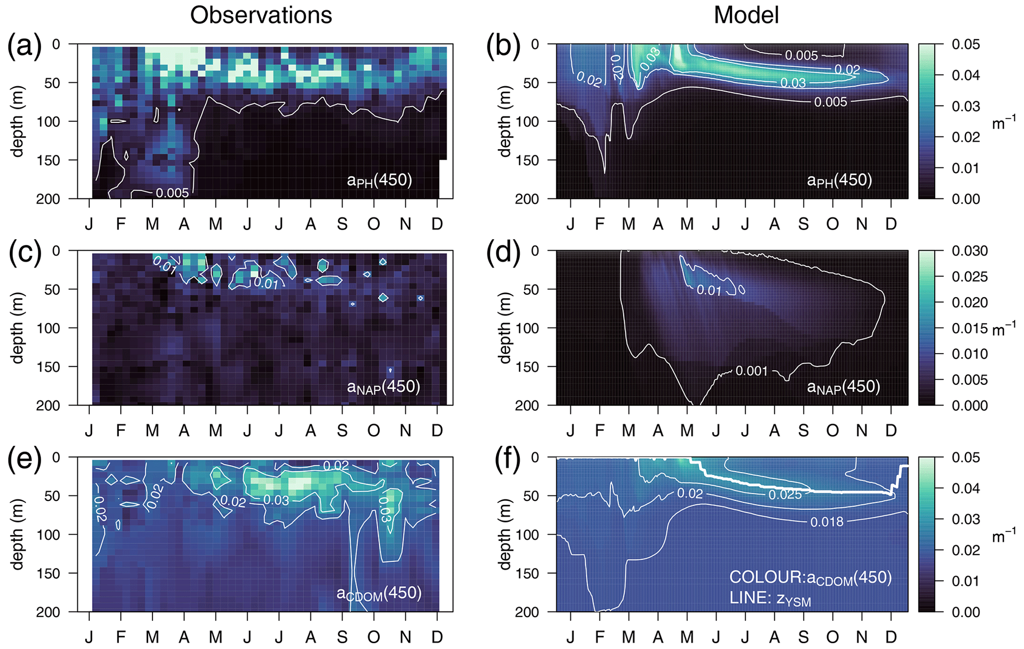
Figure 6Annually averaged vertical profiles as a function of time of (a–b) aPH(450), (c–d) aNAP(450), and (e–f) aCDOM(450), obtained from observations at the BOUSSOLE site (a, c, e) and from the optimized simulation (b, d, f). The thick line in (f) represents the depth of the yellow-substance maximum (zYSM) (depth of maximum aCDOM(400) above the 1028.88 isopycnal).
3.2.2 Light absorption budget
The relative contributions of CDOM, phytoplankton, and detritus to the total non-water light absorption at 450 nm are shown for the optimized simulation at the BOUSSOLE site in Fig. 10. During the 4-year simulation, the contribution of CDOM to the light absorption budget in the entire water column down to 100 m varied between 12 % and 99 %, with an average value of 64 %. At the surface (Fig. 10a), detritus was the minor contributor to the absorption budget (1 % to 10 %). Phytoplankton was the major absorbing substance only during the bloom in March and April, whereas aCDOM(450) dominated the rest of the year and contributed more than 50 % to the light absorption. This dominance even held in summer and fall when aCDOM(450) was minimal as a result of photobleaching (Fig. 6f). In accordance with the results reported by Organelli et al. (2014), the surface waters of BOUSSOLE can therefore be classified as CDOM type for most of the year, except for the algal bloom in March and April. In the DCM (Fig. 10b), on the other hand, with the exception of a few short mixing periods, aPH(450) always contributed the most to absorption but never exceeded 60 %. Detritus was still a minor component (1 % to 16 %), and aCDOM(450) varied between a minimum of 30% in May and a maximum of 60 %–70 % in winter. Note that the depth of the YSM was consistently about 5 m shallower than the DCM (Fig. 8 in spring, summer and fall). Even though the maximum values are not exactly at the DCM, aCDOM(450) is an important contributor to total absorption in this layer as the configuration of the optimized model is able to reproduce the formation of a CDOM subsurface maximum in spring that progressively intensifies throughout the summer, closely connected to the DCM.
3.2.3 Bio-optical relationships with aCDOM(λ)
The overall relationship between TChl a and aCDOM(λ), shown in Fig. 11a, reflects the covariation of these variables over vertical and seasonal scales. In fact, the optimized simulation showed minimum aCDOM(450) values of 0.018 m−1 (see also Fig. 6f) with very low TChl a concentrations, in agreement with data observed at the BOUSSOLE site. aCDOM(450) also tended to increase with TChl a concentrations, but the variability was large, with aCDOM(450) ranging from 0.025 to 0.07 m−1 for TChl a values equal to 1 mg m−3 (Fig. 11a). Furthermore, in agreement with Organelli et al. (2014), data shown in Fig. 11a were generally above the relationships proposed by Morel and Gentili (2009b) and Bricaud et al. (2010), derived from a global bio-optical model in the first case and from in situ measurements collected in the southeast Pacific Ocean in the second one. The main reason is the higher-than-average contribution of CDOM for a given Chl a content in the Mediterranean Sea in contrast to other oceans. Both TChl a and aCDOM(450) were used as observations in the optimization; therefore, the emergence of such a relationship was expected.
The optimized model configuration also allowed the emergence of bio-optical relationships with unobserved variables, such as DOC. The simulated aCDOM(250) as a function of DOC concentration showed a fairly linear relationship (Fig. 11b). The same relationships found by Catalá et al. (2018) and Galletti et al. (2019) (grey areas and lines in Fig. 11b) were based on in situ measurements collected over the entire Mediterranean Sea in April–May of different years. Our modelled data for spring show a good agreement with their samples taken in the upper part of the water column (with aCDOM(250) values larger than 0.9 m−1), while our modelled data for fall–winter agree better with samples taken below 200 m (aCDOM(250) values smaller than 1 m−1); this was a period when the water column was more homogeneous and when the values of both DOC (Fig. 5a) and aCDOM(λ) (Fig. 6f) in the superficial part were more similar to those in the deep part of the water column. Note that Catalá et al. (2018) and Galletti et al. (2019) reported aCDOM(λ) values at 254 nm, while modelled data report aCDOM(λ) values in the 250 nm waveband that range from 187.5 to 312.5 nm.
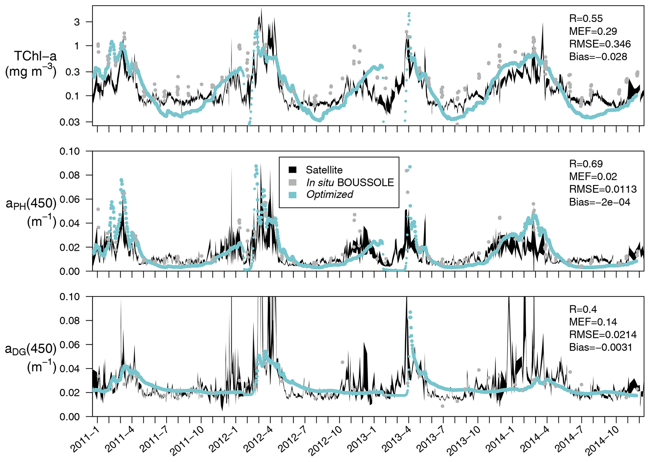
Figure 7Time series (January 2011 to December 2014) at the BOUSSOLE site of TChl a (mg m−3), aPH(450), and aDG(450) averaged over the first optical depth (calculated as ). The optimized simulation (in blue) is compared to the same satellite-retrieved products at 443 nm (in black) reporting the correlation coefficient (R), the modelling efficiency (MEF), the root mean squared error (RMSE), and the average error (bias), all calculated following Stow et al. (2009). Comparable variables measured at the BOUSSOLE site are shown for reference (grey dots).
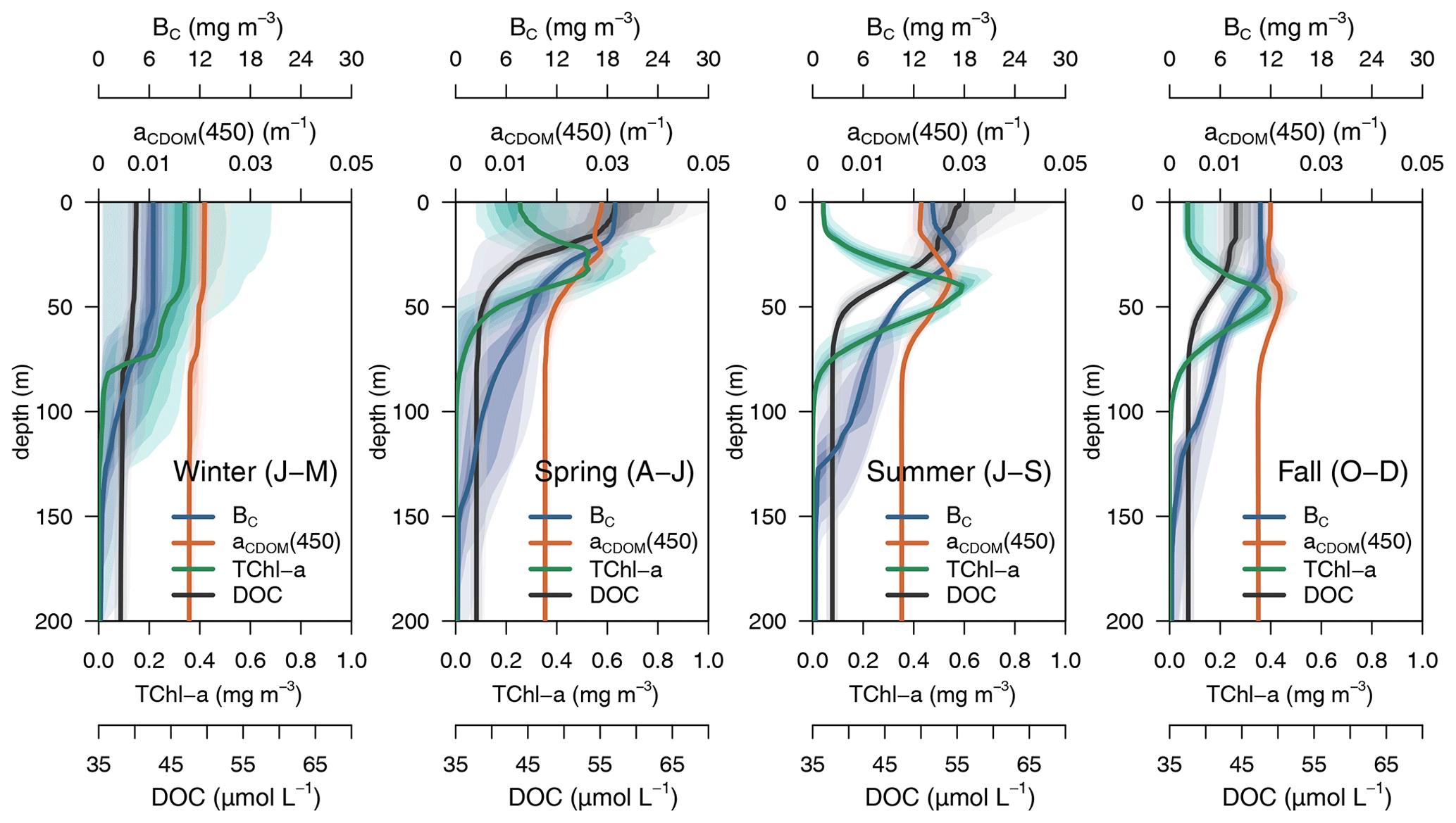
Figure 8Seasonal vertical profiles of phytoplankton TChl a, aCDOM(450), bacterial biomass, and DOC. Solid lines show the median value for the season of 4 years (2011 to 2014), and the coloured areas show the percentiles in 10 % steps from darker to lighter.
3.3 Sources of CDOM
In this final section of results, using a series of hypothesis-testing experiments (Table 2), we investigated the mechanisms that determine the vertical and temporal patterns of CDOM distribution at the BOUSSOLE site. We step through two aspects: the biogenic in situ production of biodegradable CDOM (EXP-Biology, Sect. 3.3.1) and the role of CDOM of allochthonous origin in maintaining CDOM concentrations in the surface ocean (EXP-Physics, Sect. 3.3.2).
3.3.1 In situ production of CDOM and synchronization with phytoplankton Chl a
EXP-Biology focuses on the physiological processes affecting CDOM production by phytoplankton, examining which is the coloured fraction of the total DOC of phytoplankton origin (Eq. 5). In the optimized simulation, the parameters for the production of by phytoplankton ranged from 3.2 % to 8.9 % (, , ), except for P(DINO), whose value did not converge (Appendix A). These parameters, regulated by , represent which fraction of the leakage is coloured, whereas DOC from exudation is assumed to be non-coloured. Therefore, the fraction : in the optimized simulation was variable in time and depth for two reasons: (1) it depends on the relative proportions of DOC from leakage or exudation, and (2) it depends on the θ to ratio of phytoplankton. Two additional simulations used a constant fraction of CDOM in the leakage flux (constant leakage ratio, Table 2) and a constant fraction of CDOM in the total dpp flux (constant dpp ratio, Table 2), setting these CDOM fractions to 6.2 % and 1.8,%, respectively, which are the average values obtained from the optimized simulation. The constant percentage values in the constant leakage ratio and the constant dpp ratio were chosen to homogenize the values of at the beginning of the year between the formulations and to highlight the vertical and temporal differences in between the three formulations.
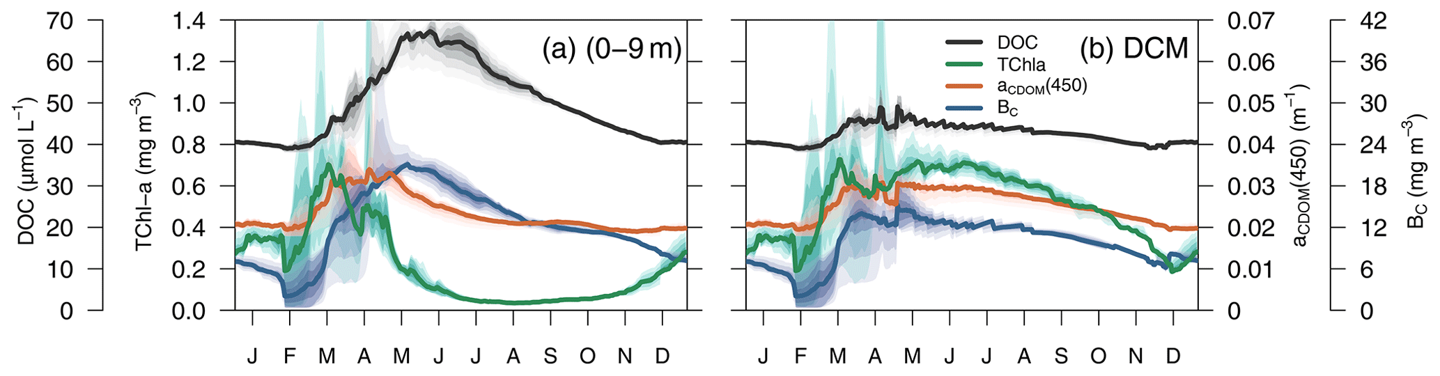
Figure 9Simulated annual evolution of phytoplankton TChl a, aCDOM(450), bacterial biomass (BC), and DOC at (a) the surface (0–9 m) and at (b) the depth of DCM. The solid lines show the average of the year from 2011 to 2014, and the coloured areas show the interannual variability.
Figure 12a shows the percentage of CDOM flux with respect to the total DOC flux ( at the surface (0–9 m) and at the depth of the DCM in the three simulations of EXP-Biology. In the constant-leakage-ratio simulation, when the sub-surface Chl a maximum develops in March–April, the proportions of CDOM production differ between the surface (1 %) and the DCM (3 %) as nutrient availability begins to decrease at the surface compared to the DCM. This difference remained fairly stable until the next mixing, except for an increase to 4 % in the DCM at the end of November. In the optimized simulation, the fraction of CDOM at the surface and at the DCM also differs from March onwards, but the percentages are lower in spring and summer (0.5 % and 2 %, respectively) and gradually increase in fall and winter as light intensity decreases and phytoplankton photoacclimate accordingly. In terms of production flux, this means that, whereas the constant-dpp-ratio simulation is the one producing more at the surface and less at the DCM (Fig. 12b vs. 12c), the constant-leakage-ratio simulation increases substantially CDOM production in the DCM compared to the other two (Fig. 12c), and the optimized simulation substantially decreases CDOM production at the surface (Fig. 12b). With respect to the observable variable aCDOM(450), the optimized formulation is able to reproduce the dynamics of aCDOM(450) at the surface during the transition from the winter productive phase to the summer better than the other two (Fig. 12d), while the constant-leakage-ratio simulation captures the dynamics of the DCM in summer quite similarly to the optimized one, suggesting that nutrient regulation predominantly determines the dynamics in the DCM (Fig. 12e).
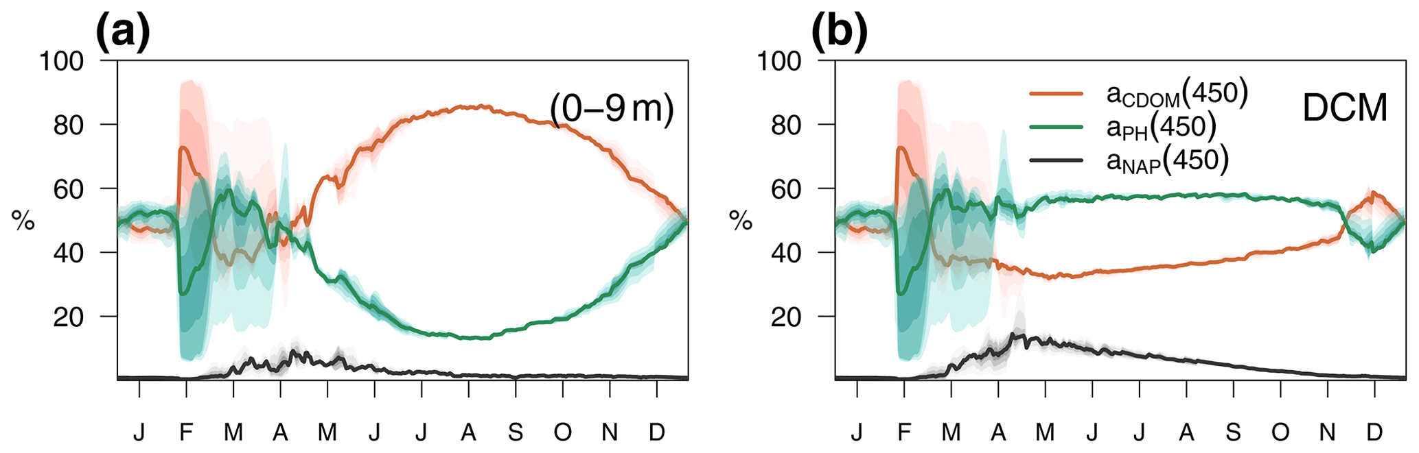
Figure 10Annual cycle of the relative contributions of CDOM, phytoplankton, and detritus to total non-water light absorption at 450 nm (a) in the first 0–9 m and (b) at the DCM of the BOUSSOLE site. The solid lines show the annual average from 2011 to 2014, and the coloured areas show the interannual variability.
3.3.2 The role of allochthonous CDOM and/or mediation by bacteria
In the optimized simulation, the deep inventory of replenishes the surface during mixing and is slowly photobleached (bX(3)=0.00119 d−1 and IX(3)=50 µE m−2 d−1, Appendix A). The optimized value of bX(3) was much lower than the prescribed value for the labile and semi-labile pools (0.167 d−1). In EXP-Physics (Fig. 13), we investigated whether maintaining the prescribed bleaching rate while increasing local production could have an equivalent effect. The optimized model configuration simulated a moderate increase in bleaching rates towards the surface compared to the simulation of intense bleaching, where the bleaching parameters for were set to be equal to the other two pools (Fig. 13a, blue line vs. magenta line). In the optimized simulation, the lower degradation contributed to the minimum values of aCDOM(450) at the surface being above 0.018–0.02 m−1 throughout the year, with contributing more than 80 % of the total pool in fall–winter and around 50 % in spring (Fig. 13b, blue line). In the intense-bleaching simulation, on the other hand, where was bleached more intensively in the illuminated part of the water column and biota-produced CDOM was quadrupled, the minimum values of fall and winter were equally maintained by and , but during the productive season, and were largely overestimated (Fig. 13b, magenta line).
The intense-bleaching simulation reproduced consistent average values of aCDOM(450), though with stronger seasonal differences than the optimized simulation at depths close to the DCM (Fig. 13c). However, below the DCM, the contribution of allochthonous is smaller in the intense-bleaching simulation than in the optimized simulation, and the biotically produced CDOM cannot maintain the observed values of aCDOM(450) (Fig. 13d). These results indicate that the optimization procedure increased concentration by reducing bleaching because even a very high (4-fold) increase in local production cannot compensate. Therefore, only allochthonous sources could balance bleaching and keep aCDOM(450) larger than 0.02 m−1 throughout the year in the upper layer. We cannot rule out the possibility that this background aCDOM(450) is sustained in reality by bacterial production. Optimization decreased bX(3) instead of increasing (2.3±1.3 %), probably because increasing cannot maintain the high aCDOM(450) values observed below the DCM since bacteria are hardly present in this layer in our simulations (Fig. 8). In any case, in the optimized simulation, the above-average aCDOM(450) values are maintained by , either by allochthonous with a lower photobleaching rate than that produced by phytoplankton or by produced by bacteria. Below 150 m, the only contributor to the total pool of CDOM is in both simulations. With an initialization value for of 1.25 mg m−3 and a remineralization rate of d−1 (Legendre et al., 2015), the values of aCDOM(450) were consistent with those observed in BOUSSOLE (Fig. 13e) and reported in Organelli et al. (2014).
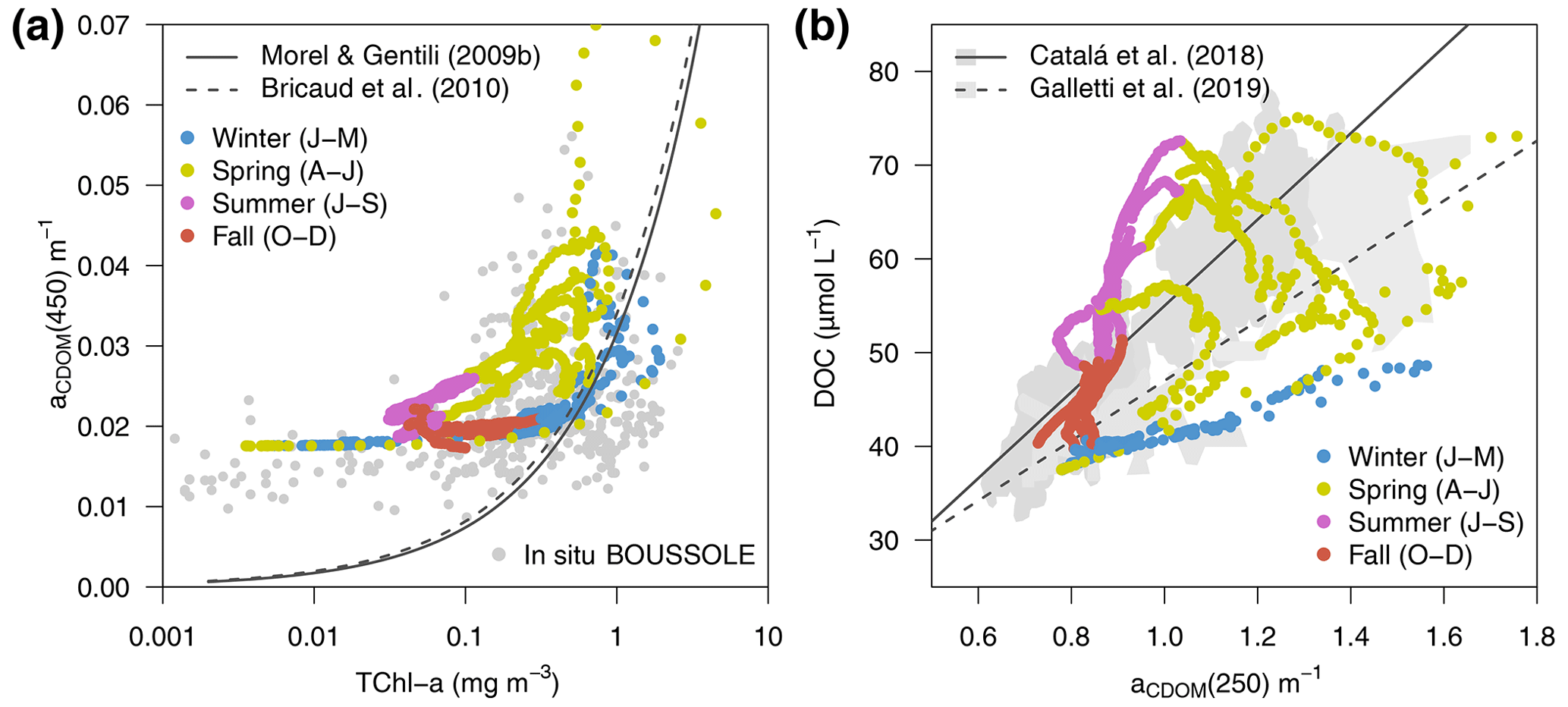
Figure 11Variations of aCDOM(λ) (a) at 450 nm (aCDOM(450)) as a function of TChl a and (b) at 250 nm (aCDOM(250)) as a function of total DOC, all simulated at the surface (0–9 m) of the BOUSSOLE site from 2011 to 2014 (dots coloured by season). The in situ TChl a and aCDOM(450) values collected at BOUSSOLE from 2011 to 2016 are displayed in the background of (a) as grey dots. The regression lines from Catalá et al. (2018) and Galletti et al. (2019) and the ranges of their reported values in the Mediterranean Sea are shown in the background of (b).
4.1 Optimization of a hydrodynamic–BGC model through a 1D fast system
Some of the uncertainties in coupled hydrodynamic–ecosystem models can be attributed to incomplete knowledge and representation of the fundamental processes being simulated (Frölicher et al., 2016) and poorly constrained parameter values (Murphy et al., 2004), especially for the BGC processes. The search for optimal parameter values by manual trial-and-error calibration or through brute-force approaches can be computationally unaffordable. Furthermore, testing parameters on an individual basis can lead to important information being missed, given parameter interactions and non-linearity of complex ecosystem models. Here we successfully applied an optimization procedure that integrates model output and observations to constrain a relatively large number of parameters in a one-dimensional configuration of the BFM. The constrained parameters contributed to improving the simulation of BGC (Chl a) and optical variables (IOPs) at the data-rich BOUSSOLE site. The use of the many observations available at this site led us to improving the simulation of bio-optical relationships that were either observed (aCDOM(450) as a function of TChl a) or not observed directly at the site (DOC as a function of aCDOM(250)) but reported by other studies in the Mediterranean Sea (Catalá et al., 2018; Galletti et al., 2019).
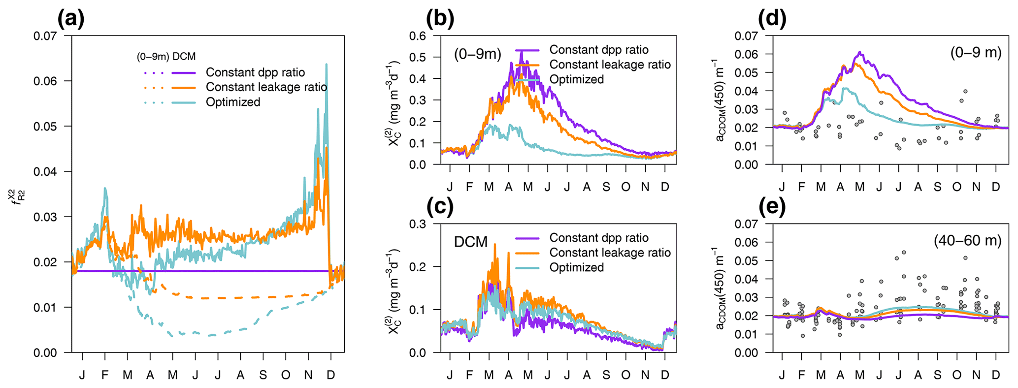
Figure 12EXP-Biology: in situ production of CDOM by phytoplankton in the optimized simulation (blue), in the simulation of constant leakage ratio where the fraction was a constant 6.2 % of leakage (orange), and in the simulation of constant dpp ratio where the fraction was a constant 1.8 % of the total dpp (purple). (a) Annual cycle of at the surface (dashed lines) and at the depth of the DCM (solid lines) in the three simulations. Annual cycle of production flux (b) averaged over the first 0–9 m and (c) in the DCM. Annual cycle of aCDOM(450) averaged in (d) the first 0–9 m and (e) between 40–60 m; the dots show aCDOM(450) values measured at the BOUSSOLE site.
Our rigorous optimization had some limits; in particular, it could not constrain all the parameters we had investigated. This was the case with the parameters for dinoflagellates (P(DINO)), which could not be constrained because this group represents only a small part of the microphytoplankton size fraction compared to diatoms (P(DIATOM)). This result indicates that the subset of observations we used may not contain enough information, which is a well-known limitation of formal optimization (Ward et al., 2010). It also suggests that the results of the optimization may vary if we use disaggregated observations for diatoms and dinoflagellates. The choice of the parameter list is also crucial. A common strategy is to optimize the parameters to which model output is more sensitive. Since we were interested in the processes that shape CDOM cycling, we chose to include in the optimization as many parameters implied in CDOM cycling as possible. Nevertheless, our results show that the optimization trajectories were, to some extent, driven by the parameters to which the model output was more sensitive. This was the case for the maximum Chl a : C quota ( of P(NANO) and P(PICO) (Fig. A2 in Appendix A), which drove the improvement in nano- and pico-phytoplankton Chl a (Fig. A1 in Appendix A) rapidly and intensively. All the parameters we investigated are involved in different processes. But interdependence and unidentified correlations between parameters can cause issues of poor identifiability; i.e. different combinations of parameters might yield the same result. Moreover, the optimized parameter values could compensate for processes that are either missing or poorly formulated in the model (e.g. the origin of in surface waters, discussed below). These two aspects imply limitations of the values obtained in this work.
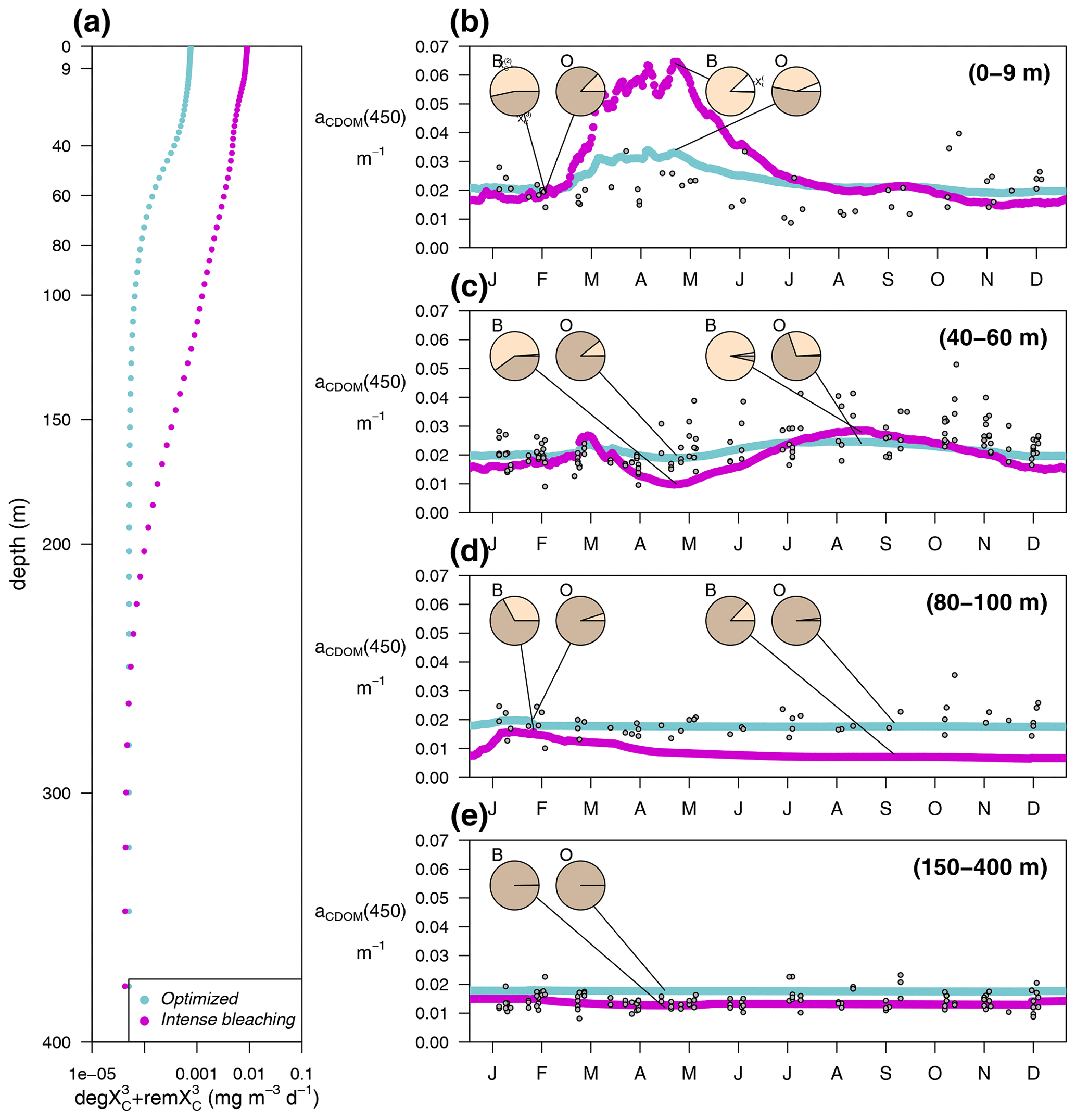
Figure 13EXP-Physics: role of in the optimized simulation (blue) and in the simulation of intense bleaching, where the bleaching rate of was set to 0.167 d−1 and where , , , and were multiplied by 4 with respect to the optimized values (pink). (a) Degradation rate of (deGX3 + remX3) as a function of depth and aCDOM(450) annual cycle averaged in depth layers between (b) 0–9 m, (c) 40–60 m, (d) 80–100 m, and (e) 150–400 m. The dots in (b–e) show aCDOM(450) observations at the BOUSSOLE site. The inset pie charts show the composition of the CDOM inventory in terms of reactivities ( in brown, in orange, and in white) at selected time points in the two simulations, intense bleaching (B) and optimized (O).
The data sets used in this work include fewer properties than the BGC model, and observations themselves are subject to errors. As a result, an excellent agreement between model and observation does not guarantee that the model's representation of unobserved properties is correct (Fennel et al., 2022). In our results, the optimized model output matched relatively well the observations provided (Figs. 4 and 5) and the same variables remotely retrieved (Fig. 7) while still being more consistent with established knowledge of processes at the BOUSSOLE site (Figs. 6 and 11) not considered in the optimization. As the results of the optimization may vary depending on how many observation types are used (Wang et al., 2020), an increasing breadth of observables will allow us to continually evaluate our model and predictions. High-frequency data collected by the BOUSSOLE project (every 15 min during daylight and at hourly intervals at night), such as Chl a fluorescence, bb(λ) of total particles, or remote-sensing reflectance above sea water, are valuable additional sources of information for further analysis. We have not tested the influence of the sampling frequency on the optimization performance. Using monthly mean profiles has been reported to be sufficient to contribute to the optimization of vertical Chl a structure and to optimize biological parameters (Shu et al., 2022; Bisson et al., 2021). But assimilating high-frequency data in a 1D model has been proven to be beneficial for inferring phytoplankton dynamics when compared to assimilating observations that are more limited in time (Kaufman et al., 2018).
CDOM-cycling models are useful only if they are flexible enough (i.e. portable) to provide accurate predictions for a wide range of conditions occurring in marine ecosystems. In that case, they can be integrated into larger 3D models of BGC cycles. The possibility of applying parameter optimization techniques in computationally efficient 1D models before using the resulting parameters in the 3D version seems advantageous. Furthermore, parameters optimized with surface data only (i.e. satellite retrieved) may present inconsistencies when simulating underwater biological fields (Wang et al., 2020). This is particularly problematic in oligotrophic regions where the deep Chl a maximum (DCM) is relatively deep and poorly correlated with surface satellite observations (Cullen, 2015; Fennel and Boss, 2003). Optimizing parameter values at intensively sampled 1D sites can overcome this problem and improve the simulation of both vertical and seasonal variability. Further analysis will be required to determine whether the optimal parameter sets from the 1D version should be applied directly in the 3D model. This decision should balance the risk of a lower agreement between model and data in 3D than in the 1D counterpart, with the opportunity to preserve key features presented in this analysis. These features include seasonal dynamics and vertical gradients and the higher-than-average CDOM light absorption coefficients (Sect. 3.1 and 3.2). Since the approximation of a 1D configuration is reasonable at the BOUSSOLE site, we do not expect that our proposed parameter values are compensating for the absence of lateral transport. However, considering that biogeochemical optimization can be influenced by specific physical forcing and possible biases in circulation dynamics (Pasquier et al., 2023), further analysis is needed to upscale the present 1D results to the 3D Mediterranean domain, where lateral contributions and vertical mixing are different and can interact differently with the optimized biogeochemical processes.
4.2 Hypothesis testing in a 1D virtual laboratory: CDOM-cycling numerical experiments
Our results provided new insights into the in situ production of semi-labile CDOM by phytoplankton. We simulated a clear seasonal and vertical structure of aCDOM(λ). This is in better agreement with observations if the proportion of coloured material in the dpp is modelled to depend on nutrient and light constraints (Fig. 12). We have proposed a simplified parameterization to account for the effects of light and nutrients on CDOM production. Nutrient limitation in relation to phytoplankton CDOM production acts through the relative proportion between leakage and dpp and seems to be the main cause of the difference in CDOM production between surface and DCM. This could reflect the fact that, when growth is limited due to low inorganic nutrient availability, the photosynthetic excess produces mainly non-coloured carbohydrates as severe N and P limitation favours the liberation of carbohydrates that do not contain these elements (Myklestad, 1995), or, simply, both higher CDOM production rates and nutrient availability occur simultaneously in the DCM (Bushaw et al., 1996; Stedmon et al., 2007; Zhang et al., 2011a). Either way, the CDOM production dependency on nutrient availability helped to reproduce the observation that increased CDOM concentrations are found at the depth of the Chl a maximum (Coble et al. 1998).
Light limitation in relation to phytoplankton CDOM production acts through the elemental ratio of Chl a : C relative to the maximum value and appears to be the main cause of the seasonality of CDOM at the surface, although it contributes to amplifying the differences between surface and DCM in CDOM production. As with nutrients, this does not necessarily represent a causal mechanism but a general pattern of high-light, low-CDOM waters. Passive leakage by diffusion through the cell membrane is controlled by cell permeability, the surface-area-to-volume ratio of the cell, and the intracellular concentration of the compound in question (Bjørrisen, 1988). Thus, our results could indeed be representative of a lower concentration of coloured material in the dpp of low-pigmented cells. However, given the inverse covariation between photosynthetic and photoprotective pigments, surface communities exposed to high light intensities that have a low θ may contain a higher proportion of photoprotective pigments. This, in principle, could contribute to the leakage of coloured molecules (e.g. carotenoids). More likely than lower CDOM production under high light, our results could be representative of increased CDOM destruction and a larger or different impact of photobleaching than assumed in our simulations. Photobleaching was likely the main cause of CDOM destruction in the surface layer from spring to summer at the BOUSSOLE site (Organelli et al., 2014), as generally observed for other oceanic waters (Coble, 2007; Bracchini et al., 2010). However, it has been found that the photochemical lability of CDOM is not necessarily related to the highest solar irradiance but depends on the accumulated light exposure (Yamashita et al., 2013; Swan et al., 2012). This may explain why the modulation of CDOM production by the photoacclimation of phytoplankton (through θ) helped to indirectly improve the effect of light intensity on CDOM concentrations.
Besides biological production in situ, our results evidence the relevance of CDOM of allochthonous origin in keeping aCDOM(450) above 0.018–0.02 m−1 throughout the year in the upper layer. It cannot be excluded that this background value of aCDOM(450) is maintained by processes in the real system that are poorly represented in the model (bacterial production) or not represented at all (other sources of allochthonous CDOM such as atmospheric deposition or advection). Nevertheless, the higher-than-average aCDOM(450) values at the surface are supported by semi-refractory CDOM (Fig. 13b), consistent with the role of atmospheric deposition in providing higher-than-average CDOM concentrations in the basin (Galletti et al., 2019). In the water column, we lack observations on the reactivity of the CDOM pool we simulated. However, our simulations mimic the results reported by Bracchini et al. (2010) in that the refractory fraction of the CDOM dominates the water below the DCM (Fig. 13d). We cannot know whether such refractory CDOM is in fact newly produced by bacteria or whether it is old CDOM vertically transported from the deep reservoir.
4.3 Conclusions and future developments
Adding optical components to BGC models greatly increases the amount of data that can be used for model validation and calibration (IOCCG, 2020). In this work, we have shown how the integration of models and observations through an optimization method provides insights into the dynamics of light-absorbing BGC products such as CDOM. Given its strong absorption of UV and blue light, the accurate simulation of CDOM cycling and its main dynamics has major implications. The potential of using an observable proxy, such as aCDOM(λ), for the retrieval of BGC products (e.g. DOC) can be significant, e.g. for carbon cycle studies and budgeting. Furthermore, the accurate simulation of the CDOM absorption band in the blue part of the spectrum helps in deciphering the mechanisms underlying the optical properties of the basin, especially in coastal and shelf waters and semi-enclosed seas such as the Mediterranean Sea. Future model developments may aim to simulate the fraction of CDOM that is able to fluoresce, i.e. fluorescent DOM, and therefore extend the points of convergence between observations and model results. Such an opportunity would be advantaged by fitting DOM fluorescence sensors on board BGC-Argo floats.
The results of the in situ production and photobleaching experiments contributed to our understanding of the main drivers of the cycling of CDOM compounds in the 1D configuration of the BFM model. These results highlight the usefulness of the 1D fast system as a virtual laboratory for hypothesis testing regarding CDOM cycling, even when proposing relatively simple parameterizations to include the effect of light and nutrients in the production of chromophoric DOM. By testing such parameterizations in the 1D configuration, we have demonstrated that they both help to represent the vertical and seasonal dynamics of CDOM at the site. They can also guide the development of further mechanistic models aimed at finding out what drives CDOM production by phytoplankton, even though observations on the relative importance of the different processes are still limited.
Twenty-five BGC and optical parameters, gathered in Table A1, were constrained (i.e. we found optimal parameter estimates with relatively small uncertainties) against observations of pico-, nano-, and microphytoplankton Chl a concentrations, aPH(450), aNAP(450), aCDOM(450), and collected at the BOUSSOLE site from 2011 to 2014. The variation in correlation coefficients (R) between the model and observations, as well as the root mean squared errors (RMSE) for all variables included in the multi-objective function (i.e. lnLikelihood), are shown in Fig. A1. All variables showed increased R and decreased RMSE compared to the observations along the optimization. The difference in lnLikelihood relative to the initial one reached 0.01 at generation 115 and 0.005 at generation 144; so, although the procedure was continued, all R's stop improving (vary by less than 0.02) after about 150 generations (nanophytoplankton Chl a was the last).
Interestingly, the improvements in the variables (RMSE reduction and R increase) and the convergences of the parameters (Fig. A2) were not homogeneous during the calibration process. Instead, the results show fast- and late-moving parameters. During the first 20 generations the main improvement was in the pico- and nano-Chl a (Fig. A1a, b), which corresponded with early constrained values of in P(PICO) and P(NANO) (Fig. A2h, m). Not all independent parameters could be well constrained. Several parameters did not converge after 180 generations. First, there was the spectral slope of the labile CDOM (. This is explained by the fact that, in our model configuration, labile CDOM is consumed as soon as it is produced; it does not accumulate, and its spectral slope has, in practice, a very limited influence on the spectral slope of the whole CDOM pool (. Second, none of the parameters of dinoflagellates (P(DINO)) converged. This is because we included an aggregate value of microphytoplanktonic Chl a in the multi-objective function (micro-Chl a), and given the preponderance of diatoms (P(DIATOM)) in this size class, varying P(DIATOM) parameters caused all changes in microphytoplankton concentration, and P(DINO) parameters had very limited influence. Two replicates of the optimization experiment were run in order to examine the robustness of the optimization procedure. Each replicate used different randomly generated seeds and therefore started from a different distribution of parameter values in the initial population. Despite slightly different optimization trajectories of the parameter values in the first 100 generations, the parameters that converged (excluding those of P(DINO) and did so to values that were between 87 %–113 % of the value reached in the main optimization experiment (Fig. A3).
Table A1List of parameters considered for optimization, with an indication of the numerical range given at the beginning of the optimization and the mean value and range obtained at the end (generation 180).
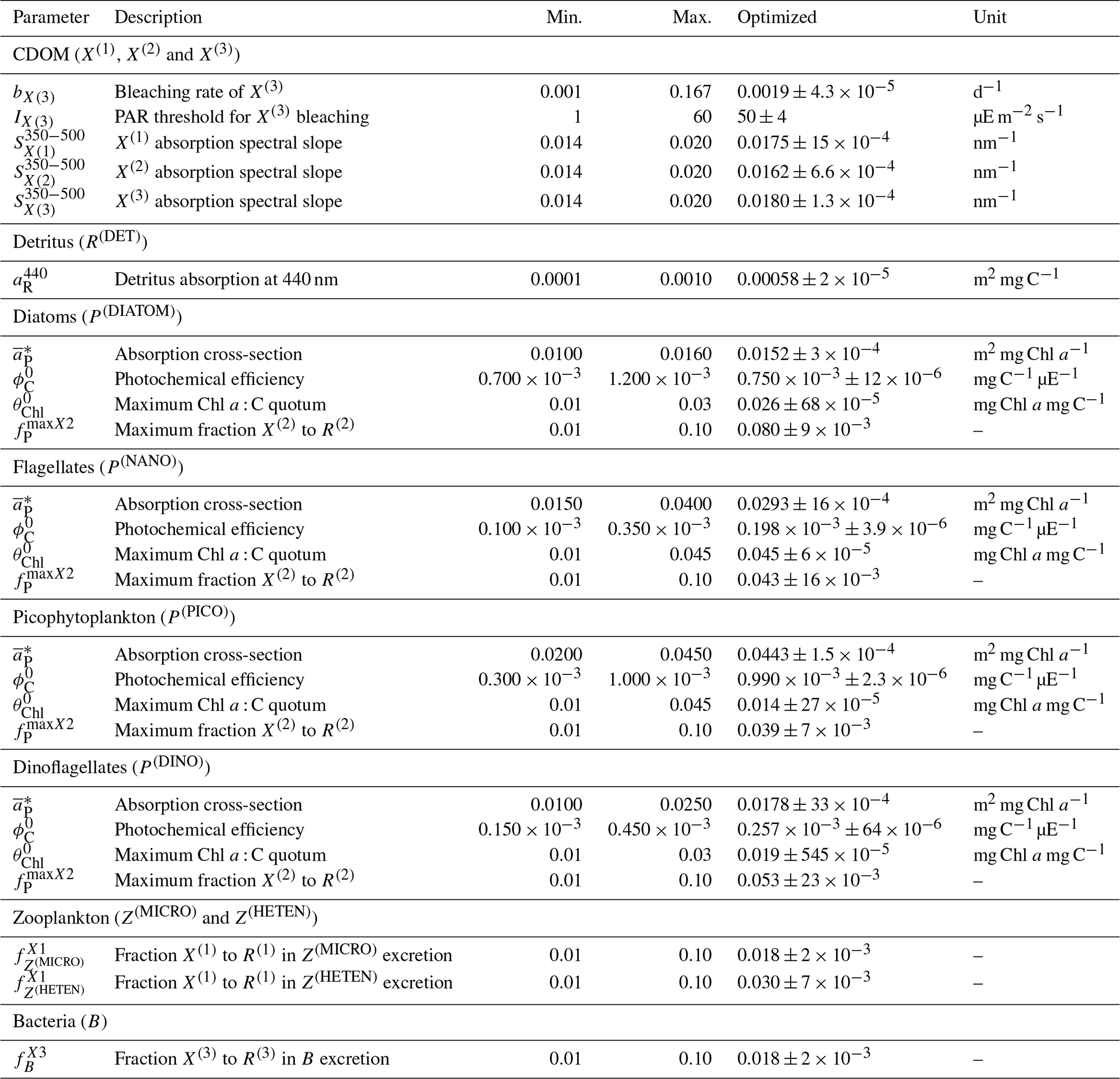
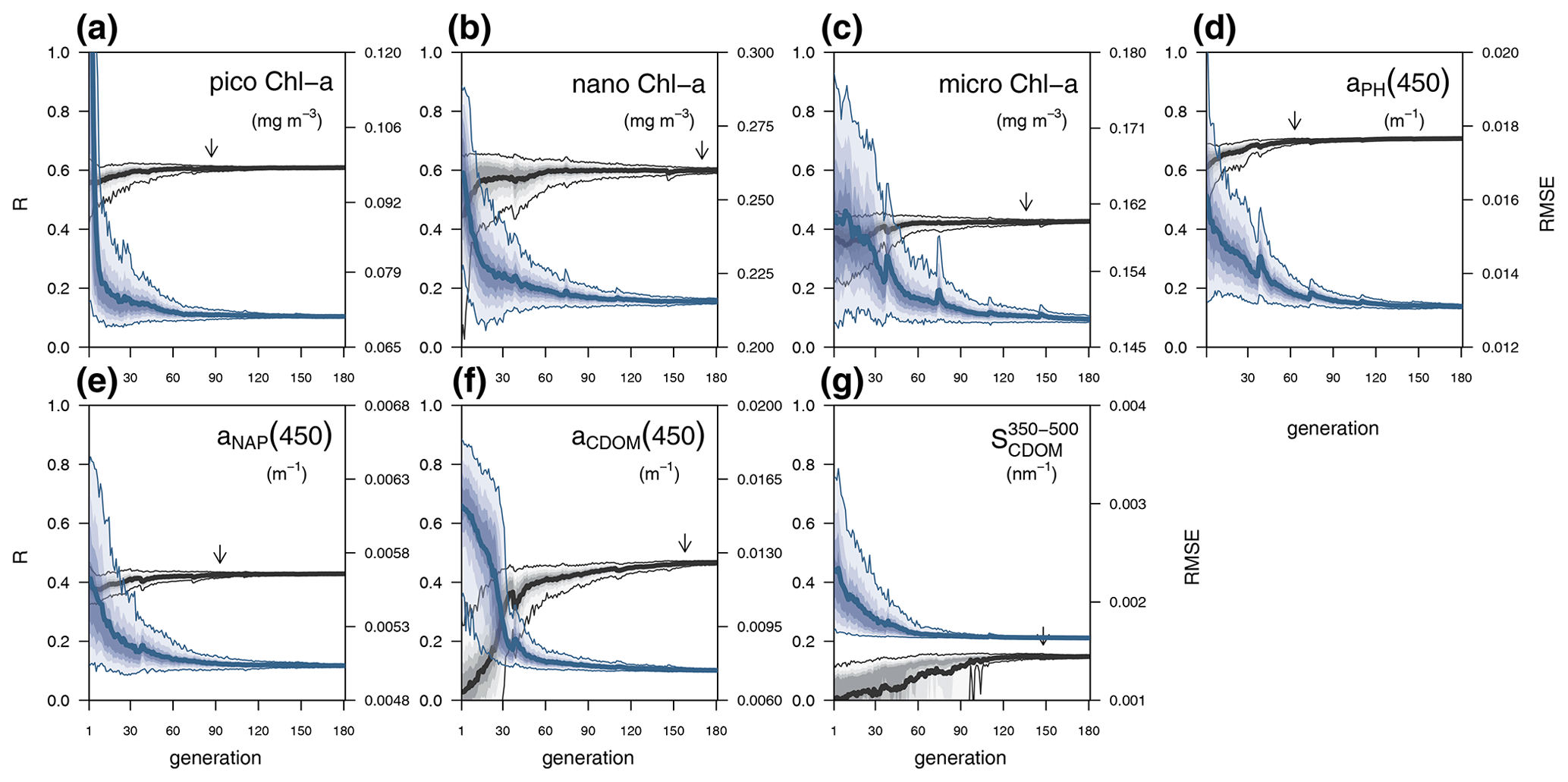
Figure A1Optimization trajectories of the fit metrics: correlation coefficient (R, grey, left axis) and root mean square error (RMSE, blue, right axis). The thick lines show the median of the distribution of the metric, and the coloured areas show the percentiles (5 %–95 %). The vertical arrows show the generation at which the range of model vs. observed R is less than 0.02.
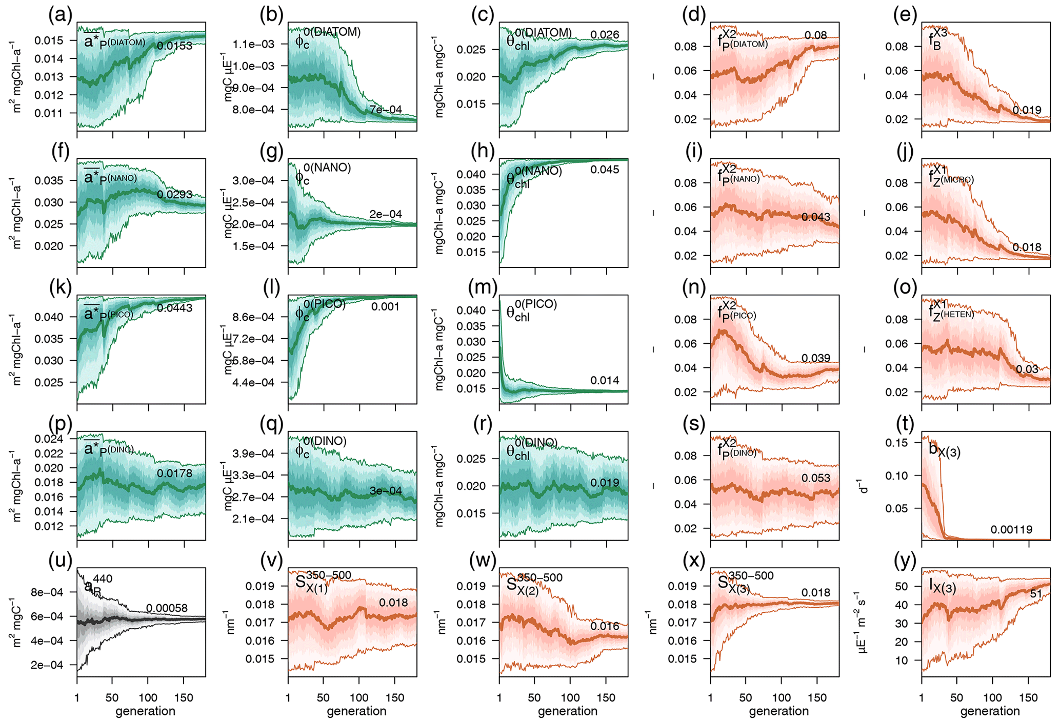
Figure A2Optimization trajectories of parameter values: phytoplankton parameters are shown in shades of green, parameters related to CDOM are shown in shades of orange, and the only detritus parameter is shown in grey. The thick lines show the median of the distribution of parameter values, and the coloured areas show the percentiles (5 %–95 %) (see Table A1 for the exact values and ranges at convergence).
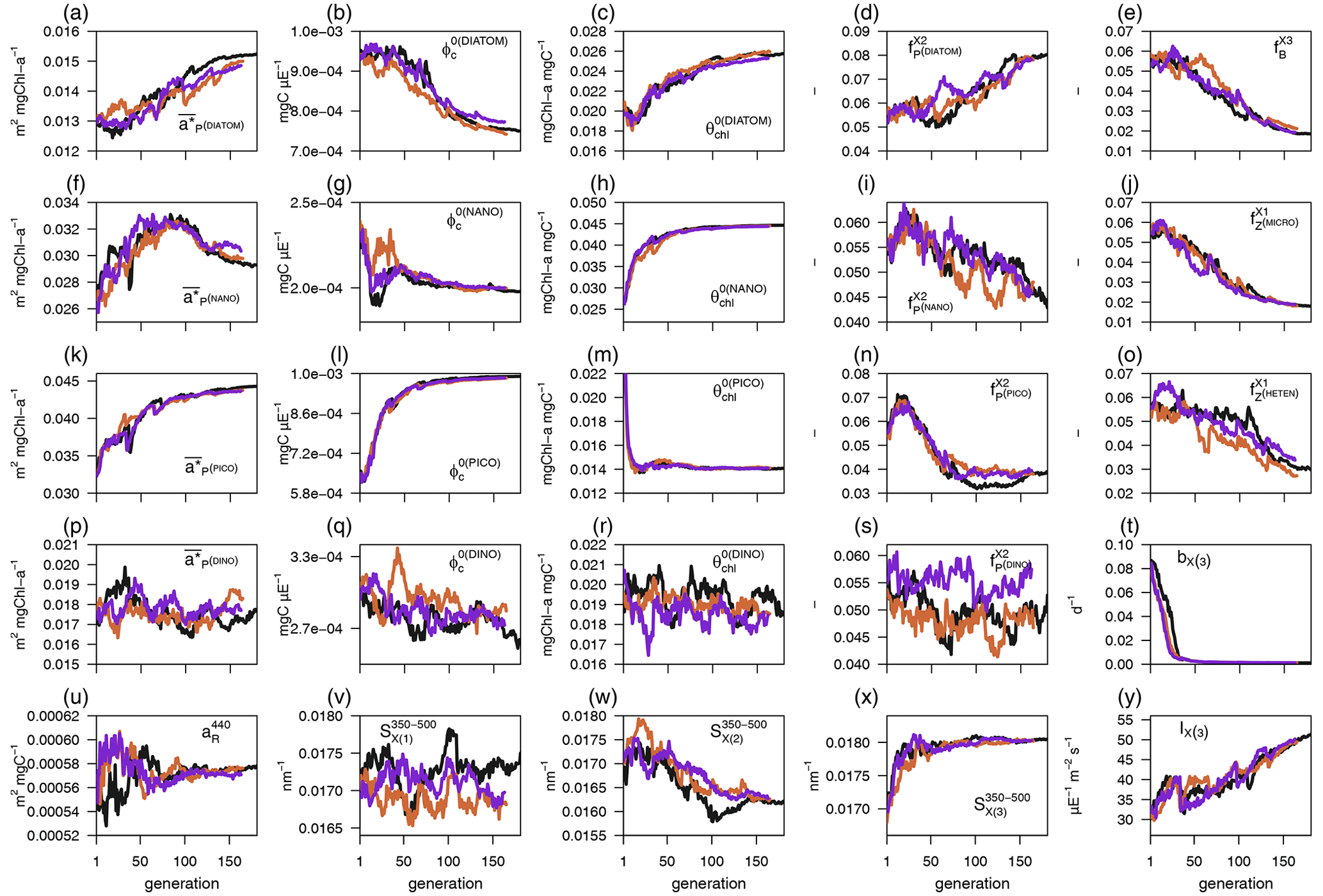
Figure A3Trajectories of parameter median values in three optimization replicates: (black) optimization experiment shown in Fig. A2 and used in the main text simulations, (orange) replicate 1 (165 generations), and (purple) replicate 2 (164 generations). Note that the scale of the y axis is zoomed in with respect to Fig. A2 to highlight differences among the median trajectories.
The GOTM code is available at https://doi.org/10.5281/zenodo.4896611 (Bolding et al., 2021). The FABM code is available at https://doi.org/10.5281/zenodo.8424553, (Bruggeman and Bolding, 2021). The BFM code adapted to work under the FABM convention is available at https://doi.org/10.5281/zenodo.10075551 (Álvarez et al., 2023), and the bio-optical model is available at https://doi.org/10.5281/zenodo.10075682 (Lazzari, 2023). ParSAC is available from PyPI and can be installed by executing the command pip install parsac < – user >; it requires Parallel Python. The 1D setup where the simulations presented can be run and the configuration files for the optimization can be obtained from https://doi.org/10.5281/zenodo.10067424 (Álvarez, 2023a).
The gridded product of temperature and salinity at DYFAMED was obtained from the OceanSITES Global Data Assembly Centre via ftp by choosing the option “Connect as Guest”.(ftp://ftp.ifremer.fr/ifremer/oceansites, last access: 22 November 2021). Nitrate, nitrite, and phosphate concentrations at DYFAMED were obtained from https://doi.org/10.17882/43749 (Coppola et al., 2021). Chl a and HPLC data at BOUSSOLE are available from http://www.obs-vlfr.fr/Boussole/html/boussole_data/other_useful_files.php (last access: 29 November 2022, Antoine and Vellucci, 2022). IOP data at BOUSSOLE are available upon request to IMEV. Satellite data are available from the EU Copernicus Marine Service at https://doi.org/10.48670/moi-00299 (E.U. Copernicus Marine Service Information, 2022). The results of the numerical simulations can be found at https://doi.org/10.5281/zenodo.7628060 (Álvarez, 2023b), and scripts for data analysis and visualization are available through https://doi.org/10.5281/zenodo.10068885 (Álvarez, 2023c). The analysis of model output has been performed with R 4.0.5 using the packages RNetCDF 2.5–2 and RSQLite 2.2.12 for importing data; abind 1.4–5, akima 0.6-2.1, chron 2.3-56, lubridate 1.8.0, Hmisc 4.5–0, and stringr 1.4.1 for data analysis; and plot3D 1.3, unikn 0.6.0, and viridisLite 0.4.1 for visualization (all publicly available in CRAN).
EÁ, GC, and PL conceptualized the research; KB provided support for GOTM; JB provided support for FABM and ParSAC: EÁ, GC, AT, JB, and PL completed the porting of BFM to FABM; VV and DA provided observational data; EÁ performed the optimization and simulations, did the analysis, and wrote the original draft of the paper. GC, SC, and PL provided funding through the SEAMLESS and NECCTON projects, and VV and DA provided funding through the BOUSSOLE project. All the authors contributed to writing, reviewing, and editing and approved the final paper.
At least one of the (co-)authors is a member of the editorial board of Biogeosciences. The peer-review process was guided by an independent editor, and the authors also have no other competing interests to declare.
Publisher’s note: Copernicus Publications remains neutral with regard to jurisdictional claims made in the text, published maps, institutional affiliations, or any other geographical representation in this paper. While Copernicus Publications makes every effort to include appropriate place names, the final responsibility lies with the authors.
All simulations were conducted on the GALILEO100 supercomputing facility at the CINECA consortium; we acknowledge CINECA for providing high-performance computing resources and support through the IscrB_3DSBM and tra21_seamless projects. Satellite products were provided by the Copernicus Marine Service, implemented by Mercator Ocean in the framework of a delegation agreement with the European Union. The BOUSSOLE project was funded by the Centre National d'Etudes Spatiales (CNES) and the European Space Agency (ESA) and was supported by the French Oceanographic Fleet (FOF). We are grateful to Emilie Diamond and Melek Golbol for conducting monthly cruises, to Annick Bricaud for CDOM analyses, and to Joséphine Ras and Céline Dimier for the phytoplankton pigment analyses (SAPIGH analytical platform of the Laboratoire d'Océanographie de Villefranche, CNRS, France). The DYFAMED time series have been provided by the Institut de la Mer de Villefranche (Laurent Coppola), the MOOSE observing network. Data were collected and made freely available by the international OceanSITES project and the national programmes that contribute to it. We sincerely appreciate the constructive feedback and valuable suggestions of two anonymous reviewers, which helped us to improve the quality of the paper.
This research has been supported by the European Commission, Horizon 2020 Framework Programme (grant no. 101004032); the European Commission, HORIZON EUROPE Framework Programme (grant no. 101081273); the Partnership for Advanced Computing in Europe AISBL (grant no. HPC-TRES); the Centre National d'Etudes Spatiales (grant no. Bouée pour l'acquisition de Séries Optiques à Long Terme (BOUSSOLE)); the European Space Agency (grant no. Bouée pour l'acquisition de Séries Optiques à Long Terme (BOUSSOLE)); the Flotte Océanographique Française (grant no. Bouée pour l'acquisition de Séries Optiques à Long Terme (BOUSSOLE)); and the Centre National de la Recherche Scientifique (grant no. MOOSE observing network).
This paper was edited by Yuan Shen and reviewed by two anonymous referees.
Aas, E.: Two-stream irradiance model for deep waters, Appl. Opt., 26, 2095–2101, https://doi.org/10.1364/AO.26.002095, 1987.
Ackleson, S. G., Balch, W. M., and Holligan, P. M.: Response of water-leaving radiance to particulate calcite and chlorophyll a concentrations: a model for Gulf of Maine coccolithophore blooms, J. Geophys. Res., 99, 7483–7500, https://doi.org/10.1029/93JC02150, 1994.
Álvarez, E., Lazzari, P., and Cossarini, G.: Phytoplankton diversity emerging from chromatic adaptation and competition for light, Prog. Oceanogr., 204, 102789, https://doi.org/10.1016/j.pocean.2022.102789, 2022.
Álvarez, E.: Setup of GOTM-FABM-BFM for 1D simulations at the BOUSSOLE site (v1.0.0), Zenodo [code], https://doi.org/10.5281/zenodo.10067424, 2023a.
Álvarez, E.: Results set of GOTM-FABM-BFM 1D simulations at the BOUSSOLE site, Zenodo, [data set], https://doi.org/10.5281/zenodo.7628060, 2023b.
Álvarez, E.: Scripts for data analysis and visualization of GOTM-FABM-BFM simulations at the BOUSSOLE site. Zenodo, [data set], https://doi.org/10.5281/zenodo.10068885, 2023c.
Álvarez, E., Teruzzi, A., Lazzari, P., Cossarini, G., and Bruggeman, J.: Biogeochemical Flux Model (BFM) for FABM (1.0). Zenodo [code], https://doi.org/10.5281/zenodo.10075551, 2023.
Antoine, D. and Vellucci, V.: BOUSSOLE project: HPLC dataset, [data set], http://www.obs-vlfr.fr/Boussole/html/boussole_data/other_useful_files.php (last access: 29 November 2022), 2022.
Antoine, D., Chami, M., Claustre, H., D'Ortenzio, F., Morel, A., Bécu, G., Gentili, B., Louis, F., Ras, J., Roussier, E., Scott, A. J., Tailliez, D., Hooker, S. B., Guevel, P., Desté, J. F., Dempsey, C., and Adams, D.: BOUSSOLE: A Joint CNRS-INSU, ESA, CNES and NASA Ocean Color Calibration and Validation Activity, NASA Technical Memorandum No. 2006, 214147, Greenbelt, 2006.
Arhonditsis, G. B. and Brett, M. T.: Evaluation of the current state of mechanistic biogeochemical modeling, Mar. Ecol. Prog. Ser., 271, 13–26, https://doi.org/10.3354/meps271013, 2004.
Avril, B.: DOC dynamics in the northwestern Mediterranean Sea (DYFAMED site), Deep-Sea Res. Pt. II, 49, 2163–2182, https://doi.org/10.1016/S0967-0645(02)00033-4, 2002.
Azam, F., Fenchel, T., Field, J. G., Gray, J. C., Meyer-Reil, L. A., and Thingstad, F.: The ecological role of water-column microbes in the sea, Mar. Ecol. Prog. Ser., 10, 257–264, https://doi.org/10.3354/meps010257, 1983.
Babin, M., Morel, A., Claustre, H., Bricaud, A., Kolber, Z., and Falkowski, P. G.: Nitrogen- and irradiance-dependent variations of the maximum quantum yield of carbon fixation in eutrophic, mesotrophic and oligotrophic marine systems, Deep-Sea Res. Pt. I, 43, 1241–1272, https://doi.org/10.1016/0967-0637(96)00058-1, 1996.
Barbieux, M., Uitz, J., Mignot, A., Roesler, C., Claustre, H., Gentili, B., Taillandier, V., D'Ortenzio, F., Loisel, H., Poteau, A., Leymarie, E., Penkerc'h, C., Schmechtig, C., and Bricaud, A.: Biological production in two contrasted regions of the Mediterranean Sea during the oligotrophic period: an estimate based on the diel cycle of optical properties measured by BioGeoChemical-Argo profiling floats, Biogeosciences, 19, 1165–1194, https://doi.org/10.5194/bg-19-1165-2022, 2022.
Barnes, M. and Antoine, D.: Proxies of community production derived from the diel variability of particulate attenuation and backscattering coefficients in the northwest Mediterranean Sea, Limnol. Oceanogr., 59, 2133–2149, https://doi.org/10.4319/lo.2014.59.6.2133, 2014.
Bayle, S., Monestiez, P., Guinet, C., and Nerini, D.: Moving toward finer scales in oceanography: Predictive linear functional model of Chlorophyll a profile from light data, Prog. Oceanogr., 134, 221–231, https://doi.org/10.1016/j.pocean.2015.02.001, 2015.
Berthon, J.-F. and Zibordi, G.: Bio-optical relationships for the northern Adriatic Sea, Int. J. Remote Sens., 25, 1527–1532, https://doi.org/10.1080/01431160310001592544, 2004.
Bidigare, R. R., Ondrusek, M. E., Morrow, J. H., and Kiefer, D. A.: In vivo absorption properties of algal pigments, in: Proc. SPIE 1302, Ocean Optics X, https://doi.org/10.1117/12.21451, 1990.
Bissett, W. P., Walsh, J. J., Dieterle, D. A., and Carder, K. L.: Carbon cycling in the upper waters of the Sargasso Sea: I. Numerical simulation of differential carbon and nitrogen fluxes, Deep-Sea Res. Pt. I, 46, 205–269, https://doi.org/10.1016/S0967-0637(98)00062-4, 1999.
Bisson, K. M., Boss, E., Werdell, P. J., Ibrahim, A., Frouin, R., and Behrenfeld, M. J.: Seasonal bias in global ocean color observations, Appl. Opt., 60, 6978, https://doi.org/10.1364/AO.426137, 2021.
Blum, M., Rozanov, V. V, Burrows, J. P., and Bracher, A.: Coupled ocean-atmosphere radiative transfer model in the framework of software package SCIATRAN: Selected comparisons to model and satellite data, Adv. Space Res., 49, 1728–1742, https://doi.org/10.1016/j.asr.2012.02.012, 2012.
Bolding, K., Bruggeman, J., Burchard, H., and Umlauf, L.: General Ocean Turbulence Model – GOTM (v6.0.2), Zenodo [code], https://doi.org/10.5281/zenodo.4896611, 2021.
Bruggeman, J. and Bolding, K.: Framework for Aquatic Biogeochemical Models (v2.0.0). Zenodo [code], https://doi.org/10.5281/zenodo.8424553, 2023.
de Boyer Montégut, C., Madec, G., Fischer, A. S., Lazar, A., and Iudicone, D.: Mixed layer depth over the global ocean: An examination of profile data and a profile-based climatology, J. Geophys. Res.-Oceans, 109, 1–20, https://doi.org/10.1029/2004JC002378, 2004.
Bracchini, L., Tognazzi, A., Dattilo, A. M., Decembrini, F., Rossi, C., and Loiselle, S. A.: Sensitivity analysis of CDOM spectral slope in artificial and natural samples: an application in the central eastern Mediterranean Basin, Aquat. Sci., 72, 485–498, https://doi.org/10.1007/s00027-010-0150-y, 2010.
Bricaud, A. and Stramski, D.: Spectral absorption coefficients of living phytoplankton and nonalgal biogenous matter: A comparison between the Peru upwelling areaand the Sargasso Sea, Limnol. Oceanogr., 35, 562–582, https://doi.org/10.4319/lo.1990.35.3.0562, 1990.
Bricaud, A., Babin, M., Claustre, H., Ras, J., and Tièche, F.: Light absorption properties and absorption budget of Southeast Pacific waters, J. Geophys. Res., 115, 1–19, https://doi.org/10.1029/2009JC005517, 2010.
Bruggeman, J. and Bolding, K.: A general framework for aquatic biogeochemical models, Environ. Modell Softw., 61, 249–265, https://doi.org/10.1016/j.envsoft.2014.04.002, 2014.
Bruggeman, J. and Bolding, K.: parsac: parallel sensitivity analysis and calibration (0.5.7), https://doi.org/10.5281/zenodo.4280520, 2020.
Burchard, H., Bolding, K., and Villarreal, M.: GOTM, a general ocean turbulence model: Theory, implementation and test cases, Report EUR 18745, 1999.
Catalá, T. S., Martínez-Pérez, A. M., Nieto-Cid, M., Álvarez, M., Otero, J., Emelianov, M., Reche, I., Arístegui, J., and Álvarez-Salgado, X. A.: Dissolved Organic Matter (DOM) in the open Mediterranean Sea, I. Basin–wide distribution and drivers of chromophoric DOM, Prog. Oceanogr., 165, 35–51, https://doi.org/10.1016/j.pocean.2018.05.002, 2018.
Ciavatta, S., Brewin, R. J. W., Skákala, J., Polimene, L., de Mora, L., Artioli, Y., and Allen, J. I.: Assimilation of Ocean-Color Plankton Functional Types to Improve Marine Ecosystem Simulations, J. Geophys. Res.-Oceans, 123, 834–854, https://doi.org/10.1002/2017JC013490, 2018.
Claustre, H., Morel, A., Hooker, S. B., Babin, M., Antoine, D., Oubelkheir, K., Bricaud, A., Leblanc, K., Quéguiner, B., and Maritorena, S.: Is desert dust making oligotrophic waters greener?, Geophys. Res. Lett., 29, 1071–1074, https://doi.org/10.1029/2001GL014056, 2002.
Coble, P. G.: Marine Optical Biogeochemistry The Chemistry of Ocean Color, Chem. Rev., 107, 402–418, https://doi.org/10.1021/cr050350+, 2007.
Copin-Montégut, G. and Avril, B.: Vertical distribution and temporal variation of dissolved organic carbon in the North-Western Mediterranean Sea, Deep-Sea Res. Pt. I, 40, 1963–1972, https://doi.org/10.1016/0967-0637(93)90041-Z, 1993.
Coppola, L., Diamond, R. E., and Carval, T.: Dyfamed observatory data, [data set] https://doi.org/10.17882/43749, 2021.
Cossarini, G., Feudale, L., Teruzzi, A., Bolzon, G., Coidessa, G., Solidoro, C., Di Biagio, V., Amadio, C., Lazzari, P., Brosich, A., and Salon, S.: High-Resolution Reanalysis of the Mediterranean Sea Biogeochemistry (1999–2019), Front. Mar. Sci., 8, 741486, https://doi.org/10.3389/fmars.2021.741486, 2021.
DeGrandpre, M. D., Vodacek, A., Nelson, R. K., Bruce, E. J., and Blough, N. V.: Seasonal seawater optical properties of the U.S. Middle Atlantic Bight, J. Geophys. Res.-Oceans, 101, 22727–22736, https://doi.org/10.1029/96JC01572, 1996.
D'Ortenzio, F., Antoine, D., and Marullo, S.: Satellite-driven modeling of the upper ocean mixed layer and air–sea CO2 flux in the Mediterranean Sea, Deep-Sea Res. Pt. I, 55, 405–434, https://doi.org/10.1016/j.dsr.2007.12.008, 2008.
Dutkiewicz, S., Hickman, A. E., Jahn, O., Gregg, W. W., Mouw, C. B., and Follows, M. J.: Capturing optically important constituents and properties in a marine biogeochemical and ecosystem model, Biogeosciences, 12, 4447–4481, https://doi.org/10.5194/bg-12-4447-2015, 2015.
E.U. Copernicus Marine Service Information: Mediterranean Sea Ocean Colour Plankton, Reflectance, Transparency and Optics MY L3 daily observations, [data set], https://doi.org/10.48670/moi-00299, 2022.
Falls, M., Bernardello, R., Castrillo, M., Acosta, M., Llort, J., and Galí, M.: Use of genetic algorithms for ocean model parameter optimisation: a case study using PISCES-v2_RC for North Atlantic particulate organic carbon, Geosci. Model Dev., 15, 5713–5737, https://doi.org/10.5194/gmd-15-5713-2022, 2022.
Fennel, K., Mattern, J. P., Doney, S. C., Bopp, L., Moore, A. M., Wang, B., and Yu, L.: Ocean biogeochemical modelling, Nat. Rev. Methods Primers, 2, 76, https://doi.org/10.1038/s43586-022-00154-2, 2022.
Frölicher, T. L., Rodgers, K. B., Stock, C. A., and Cheung, W. W. L.: Sources of uncertainties in 21st century projections of potential ocean ecosystem stressors, Global Biogeochem. Cy., 30, 1224–1243, https://doi.org/10.1002/2015GB005338, 2016.
Gallegos, C. L., Werdell, P. J., and McClain, C. R.: Long-term changes in light scattering in Chesapeake Bay inferred from Secchi depth, light attenuation, and remote sensing measurements, J. Geophys. Res.-Oceans, 116, 1–19, https://doi.org/10.1029/2011JC007160, 2011.
Galletti, Y., Gonnelli, M., Retelletti Brogi, S., Vestri, S., and Santinelli, C.: DOM dynamics in open waters of the Mediterranean Sea: New insights from optical properties, Deep-Sea Res. Pt. I, 144, 95–114, https://doi.org/10.1016/j.dsr.2019.01.007, 2019.
Gitelson, A., Karnieli, A., Goldman, N., Yacobi, Y. Z., and Mayo, M.: Chlorophyll estimation in the Southeastern Mediterranean using CZCS images: adaptation of an algorithm and its validation, J. Mar. Syst., 9, 183–290, https://doi.org/10.1016/S0924-7963(95)00047-X, 1996.
Golbol, M., Vellucci, V., and Antoine, D.: BOUSSOLE, https://doi.org/10.18142/1, 2000.
Gregg, W. W.: A Coupled Ocean–Atmosphere Radiative Model for Global Ocean Biogeochemical Model, NASA Technical Report Series on Global Modeling and Data Assimilation, NASA/TM- 2002-104606, 22, 2002.
Gregg, W. W. and Rousseaux, C. S.: Simulating PACE Global Ocean Radiances, Front. Mar. Sci., 4, 1–19, https://doi.org/10.3389/fmars.2017.00060, 2017.
Hickman, A. E., Dutkiewicz, S., Williams, R. G., and Follows, M. J.: Modelling the effects of chromatic adaptation on phytoplankton community structure in the oligotrophic ocean, Mar. Ecol. Prog. Ser., 406, 1–17, https://doi.org/10.3354/meps08588, 2010.
IOCCG: Synergy between Ocean Colour and Biogeochemical/Ecosystem Models, edited by: Dutkiewicz, S., International Ocean-Colour Coordinating Group (IOCCG), Dartmouth, NS, Canada, 184 pp., https://doi.org/10.25607/OBP-711, 2020.
Jerlov, N. G.: Optical studies of ocean waters, Rep. Swed. deep Sea Exped, 1947–1948, 3, 1–59, 1951.
Kaufman, D. E., Friedrichs, M. A. M., Hemmings, J. C. P., and Smith Jr., W. O.: Assimilating bio-optical glider data during a phytoplankton bloom in the southern Ross Sea, Biogeosciences, 15, 73–90, https://doi.org/10.5194/bg-15-73-2018, 2018.
Kriest, I., Sauerland, V., Khatiwala, S., Srivastav, A., and Oschlies, A.: Calibrating a global three-dimensional biogeochemical ocean model (MOPS-1.0), Geosci. Model Dev., 10, 127–154, https://doi.org/10.5194/gmd-10-127-2017, 2017.
Kuhn, A. M. and Fennel, K.: Evaluating ecosystem model complexity for the northwest North Atlantic through surrogate-based optimization, Ocean Model, 142, 101437, https://doi.org/10.1016/j.ocemod.2019.101437, 2019.
Lazzari, P.: Forward_Adjoint: three-stream solver (v1.0). Zenodo [code], https://doi.org/10.5281/zenodo.10075682, 2023.
Lazzari, P., Solidoro, C., Ibello, V., Salon, S., Teruzzi, A., Béranger, K., Colella, S., and Crise, A.: Seasonal and inter-annual variability of plankton chlorophyll and primary production in the Mediterranean Sea: a modelling approach, Biogeosciences, 9, 217–233, https://doi.org/10.5194/bg-9-217-2012, 2012.
Lazzari, P., Salon, S., Terzić, E., Gregg, W. W., D'Ortenzio, F., Vellucci, V., Organelli, E., and Antoine, D.: Assessment of the spectral downward irradiance at the surface of the Mediterranean Sea using the radiative Ocean-Atmosphere Spectral Irradiance Model (OASIM), Ocean Sci., 17, 675–697, https://doi.org/10.5194/os-17-675-2021, 2021a.
Lazzari, P., Álvarez, E., Terzić, E., Cossarini, G., Chernov, I., D'Ortenzio, F., and Organelli, E.: CDOM spatiotemporal variability in the Mediterranean Sea: a modelling study, J. Mar. Sci. Eng., 9, 176, https://doi.org/10.3390/jmse9020176, 2021b.
Lee, Z. P., Carder, K. L., and Arnone, R. A.: Deriving inherent optical properties from water color: a multiband quasi-analytical algorithm for optically deep waters, Appl. Opt., 41, 4957–4964, https://doi.org/10.1364/AO.41.005755, 2002.
Legendre, L., Rivkin, R. B., Weinbauer, M. G., Guidi, L., and Uitz, J.: The microbial carbon pump concept: Potential biogeochemical significance in the globally changing ocean, Prog. Oceanogr., 134, 432–450, https://doi.org/10.1016/j.pocean.2015.01.008, 2015.
Mattern, J. P. and Edwards, C. A.: Simple parameter estimation for complex models – Testing evolutionary techniques on 3-dimensional biogeochemical ocean models, J. Mar. Syst., 165, 139–152, https://doi.org/10.1016/j.jmarsys.2016.10.012, 2017.
Mélin, F. and Vantrepotte, V.: How optically diverse is the coastal ocean?, Remote Sens Environ, 160, 235–251, https://doi.org/10.1016/j.rse.2015.01.023, 2015.
Mignot, A., Claustre, H., D'Ortenzio, F., Xing, X., Poteau, A., and Ras, J.: From the shape of the vertical profile of in vivo fluorescence to Chlorophyll-a concentration, Biogeosciences, 8, 2391–2406, https://doi.org/10.5194/bg-8-2391-2011, 2011.
Mitchell, B. G.: Algorithms for determining the absorption coefficient of aquatic particulates using the quantitative filter technique (QFT), in: Ocean Optics X, 137–148, 1990.
Mitchell, B. G., Bricaud, A., Carder, K., Cleveland, J., Ferrari, G. M., Gould, R., Kahru, M., Kishino, M., Maske, H., Moisan, T., Moore, L., Nelson, N., Phinney, D., Reynolds, R. A., Sosik, H., Stramski, D., Tassan, S., Trees, C., Weidemann, A., Wieland, J. D., and Vodacek, A.: Determination of spectral absorption coefficients of particles, dissolved material and phytoplankton for discrete water samples, in: Ocean Optics Protocols For Satellite Ocean Color Sensor Validation, Revision 2. NASA Technical Memorandum 2000-209966, Chapter 12, 125–153, edited by: Fargion, G. S. and Mueller, J. L., NASA Goddard Space Flight Center, Greenbelt, Maryland, 2000.
Mopper, K. and Kieber, D. J.: Marine photochemistry and its impact on carbon cycling, in: The Effects of UV Radiation in the Marine Environment, edited by: De Mora, S., Demers, S., and Vernet, M., Cambridge University Press, 101–129, https://doi.org/10.1017/CBO9780511535444.005, 2000.
Morel, A.: Optical properties of pure water and pure sea water, in: Optical Aspects of Oceanography, edited by: Jerlov, N. G. and Nielson, E. S., Academic Press, New York, 1–24, 1974.
Morel, A. and Gentili, B.: A simple band ratio technique to quantify the colored dissolved and detrital organic material from ocean color remotely sensed data, Remote Sens Environ, 113, 998–1011, https://doi.org/10.1016/j.rse.2009.01.008, 2009a.
Morel, A. and Gentili, B.: The dissolved yellow substance and the shades of blue in the Mediterranean Sea, Biogeosciences, 6, 2625–2636, https://doi.org/10.5194/bg-6-2625-2009, 2009b.
Mühlenbruch, M., Grossart, H. P., Eigemann, F., and Voss, M.: Mini-review: Phytoplankton-derived polysaccharides in the marine environment and their interactions with heterotrophic bacteria, Environ. Microb., 20, 2671–2685, https://doi.org/10.1111/1462-2920.14302, 2018.
Murphy, J. M., Sexton, D. M. H., Barnett, D. N., Jones, G. S., Webb, M. J., Collins, M., and Stainforth, D. A.: Quantification of modelling uncertainties in a large ensemble of climate change simulations, Nature, 430, 768–772, https://doi.org/10.1038/nature02771, 2004.
Myklestad, S. M.: Release of extracellular products by phytoplankton with special emphasis on polysaccharides, Sci. Total Environ., 165, 155–164, https://doi.org/10.1016/0048-9697(95)04549-G, 1995.
Nelson, N. B. and Gauglitz, J. M.: Optical Signatures of Dissolved Organic Matter Transformation in the Global Ocean, Front. Mar. Sci., 2, 118, https://doi.org/10.3389/fmars.2015.00118, 2016.
Nelson, N. B., Siegel, D. A., and Michaels, A. F.: Seasonal dynamics of colored dissolved material in the Sargasso Sea, Deep-Sea Res. Pt. I, 45, 931–957, https://doi.org/10.1016/S0967-0637(97)00106-4, 1998.
Organelli, E., Nuccio, C., Melillo, C., and Massi, L.: Relationships between phytoplankton light absorption, pigment composition and size structure in offshore areas of the Mediterranean Sea, Adv. Ocean. Limnol., 2, 107–123, https://doi.org/10.1080/19475721.2011.607489, 2011.
Organelli, E., Bricaud, A., Antoine, D., and Uitz, J.: Multivariate approach for the retrieval of phytoplankton size structure from measured light absorption spectra in the Mediterranean Sea (BOUSSOLE site), Appl. Opt., 52, 2257, https://doi.org/10.1364/AO.52.002257, 2013.
Organelli, E., Bricaud, A., Antoine, D., and Matsuoka, A.: Seasonal dynamics of light absorption by chromophoric dissolved organic matter (CDOM) in the NW Mediterranean Sea (BOUSSOLE site), Deep-Sea Res. Pt. I, 91, 72–85, https://doi.org/10.1016/j.dsr.2014.05.003, 2014.
Oubelkheir, K., Claustre, H., Sciandra, A., and Babin, M.: Bio-optical and biogeochemical properties of different trophic regimes in oceanic waters, Limnol. Oceanogr., 50, 1795–1809, https://doi.org/10.4319/lo.2005.50.6.1795, 2005.
Oubelkheir, K., Claustre, H., Bricaud, A., and Babin, M.: Partitioning total spectral absorption in phytoplankton and colored detrital material contributions, Limnol. Ocean. Meth., 5, 384–395, https://doi.org/10.4319/lom.2007.5.384, 2007.
Pasquier, B., Holzer, M., Chamberlain, M. A., Matear, R. J., Bindoff, N. L., and Primeau, F. W.: Optimal parameters for the ocean's nutrient, carbon, and oxygen cycles compensate for circulation biases but replumb the biological pump, EGUsphere [preprint], https://doi.org/10.5194/egusphere-2023-363, 2023.
Pérez, G. L., Galí, M., Royer, S.-J., Sarmento, H., Gasol, J. M., Marrasé, C., and Simó, R.: Bio-optical characterization of offshore NW Mediterranean waters: CDOM contribution to the absorption budget and diffuse attenuation of downwelling irradiance, Deep-Sea Res. Pt. I, 114, 111–127, https://doi.org/10.1016/j.dsr.2016.05.011, 2016.
Pope, R. M. and Fry, E. S.: Absorption spectrum 380–700 nm of pure water, II. Integrating cavity measurements, Appl. Opt., 36, 8710–8723, 1997.
Ras, J., Claustre, H., and Uitz, J.: Spatial variability of phytoplankton pigment distributions in the Subtropical South Pacific Ocean: comparison between in situ and predicted data, Biogeosciences, 5, 353–369, https://doi.org/10.5194/bg-5-353-2008, 2008.
Romera-Castillo, C., Sarmento, H., Álvarez-Salgado, X. A., Gasol, J. M., and Marrasé, C.: Production of chromophoric dissolved organic matter by marine phytoplankton, Limnol. Oceanogr., 55, 446–454, https://doi.org/10.4319/lo.2010.55.1.0446, 2010.
Santinelli, C.: DOC in the Mediterranean Sea, in: Biogeochemistry of Marine Dissolved Organic Matter, edited by: Hansell, D. A. and Carlson, C. A., Academic Press, San Diego, 579–608, https://doi.org/10.1016/B978-0-12-405940-5.00013-3, 2015.
Santinelli, C., Gasparini, G. P., Nannicini, L., and Seritti, A.: Vertical distribution of dissolved organic carbon (DOC) in the Western Mediterranean Sea in relation to the hydrological characteristics, Deep-Sea Res. Pt. I, 49, 2203–2219, https://doi.org/10.1016/S0967-0637(02)00129-2, 2002.
Sauzède, R., Claustre, H., Jamet, C., Uitz, J., Ras, J., Mignot, A., and D'Ortenzio, F.: Retrieving the vertical distribution of chlorophyll a concentration and phytoplankton community composition from in situ fluorescence profiles: A method based on a neural network with potential for global-scale applications, J. Geophys. Res.-Oceans, 120, 451–470, https://doi.org/10.1002/2014JC010355, 2015.
Shu, C., Xiu, P., Xing, X., Qiu, G., Ma, W., Brewin, R. J. W., and Ciavatta, S.: Biogeochemical Model Optimization by Using Satellite-Derived Phytoplankton Functional Type Data and BGC-Argo Observations in the Northern South China Sea, Remote Sens (Basel), 14, 1297, https://doi.org/10.3390/rs14051297, 2022.
Sieburth, J. M. and Jensen, A.: Studies on algal substances in the sea. I. Gelbstoff (humic material) in terrestrial and marine waters, J. Exp. Mar. Biol. Ecol., 2, 174–189, https://doi.org/10.1016/0022-0981(68)90008-7, 1968.
Siegel, D. A., Behrenfeld, M. J., Maritorena, S., McClain, C. R., Antoine, D., Bailey, S. W., Bontempi, P. S., Boss, E. S., Dierssen, H. M., Doney, S. C., Eplee, R. E., Evans, R. H., Feldman, G. C., Fields, E., Franz, B. A., Kuring, N. A., Mengelt, C., Nelson, N. B., Patt, F. S., Robinson, W. D., Sarmiento, J. L., Swan, C. M., Werdell, P. J., Westberry, T. K., Wilding, J. G., and Yoder, J. A.: Regional to global assessments of phytoplankton dynamics from the SeaWiFS mission, Remote Sens. Environ., 135, 77–91, https://doi.org/10.1016/j.rse.2013.03.025, 2013.
Smith, R. C. and Baker, K. S.: Optical properties of the clearest natural waters (200–800 nm), Appl. Opt., 20, 177–184, https://doi.org/10.1364/AO.20.000177, 1981.
Stedmon, C. A. and Markager, S.: Tracing the production and degradation of autochthonous fractions of dissolved organic matter by fluorescence analysis, Limnol. Oceanogr., 50, 1415–1426, https://doi.org/10.4319/lo.2005.50.5.1415, 2005.
Storn, R. and Price, K.: Differential Evolution – A Simple and Efficient Heuristic for global Optimization over Continuous Spaces, J. Glob. Opt., 11, 341–359, https://doi.org/10.1023/A:1008202821328, 1997.
Stow, C. A., Jolliff, J., McGillicuddy, D. J., Doney, S. C., Allen, J. I., Friedrichs, M. A. M., Rose, K. A., and Wallhead, P.: Skill assessment for coupled biological/physical models of marine systems, J. Mar. Syst., 76, 4–15, https://doi.org/10.1016/j.jmarsys.2008.03.011, 2009.
Swan, C. M., Nelson, N. B., Siegel, D. A., and Kostadinov, T. S.: The effect of surface irradiance on the absorption spectrum of chromophoric dissolved organic matter in the global ocean, Deep-Sea Res. Pt. I, 63, 52–64, https://doi.org/10.1016/j.dsr.2012.01.008, 2012.
Teruzzi, A., Bolzon, G., Feudale, L., and Cossarini, G.: Deep chlorophyll maximum and nutricline in the Mediterranean Sea: emerging properties from a multi-platform assimilated biogeochemical model experiment, Biogeosciences, 18, 6147–6166, https://doi.org/10.5194/bg-18-6147-2021, 2021.
Terzić, E., Miró, A., Organelli, E., Kowalczuk, P., D'Ortenzio, F., and Lazzari, P.: Radiative transfer modeling with Biogeochemical-Argo float data in the Mediterranean Sea, J. Geophys. Res.-Oceans, 126, e2021JC01769, https://doi.org/10.1029/2021JC017690, 2021.
Thornton, D. C. O.: Dissolved organic matter (DOM) release by phytoplankton in the contemporary and future ocean, Eur. J. Phycol., 49, 20–46, https://doi.org/10.1080/09670262.2013.875596, 2014.
Uitz, J., Claustre, H., Morel, A., and Hooker, S. B.: Vertical distribution of phytoplankton communities in open ocean: An assessment based on surface chlorophyll, J. Geophys. Res, 111, C08005, https://doi.org/10.1029/2005JC003207, 2006.
Ulses, C., Auger, P.-A., Soetaert, K., Marsaleix, P., Diaz, F., Coppola, L., Herrmann, M. J., Kessouri, F., and Estournel, C.: Budget of organic carbon in the North-Western Mediterranean open sea over the period 2004-2008 using 3-D coupled physical-biogeochemical modeling, J. Geophys. Res.-Oceans, 121, 7026–7055, https://doi.org/10.1002/2016JC011818, 2016.
Vichi, M., Pinardi, N., and Masina, S.: A generalized model of pelagic biogeochemistry for the global ocean ecosystem, Part I: Theory, J. Mar. Syst., 64, 89–109, https://doi.org/10.1016/j.jmarsys.2006.03.006, 2007a.
Vichi, M., Masina, S., and Navarra, A.: A generalized model of pelagic biogeochemistry for the global ocean ecosystem. Part II: Numerical simulations, J. Mar. Syst., 64, 110–134, https://doi.org/10.1016/j.jmarsys.2006.03.014, 2007b.
Vichi, M., Lovato, T., Butenschön, M., Tedesco, L., Lazzari, P., Cossarini, G., Masina, S., Pinardi, N., Solidoro, C., and Zavatarelli, M.: The Biogeochemical Flux Model (BFM): Equation Description and User Manual. BFM version 5.2. BFM Report series N. 1, Release 1.2, Bologna, 2020.
Volpe, G., Santoleri, R., Vellucci, V., Ribera d'Alcalà, M., Marullo, S., and D'Ortenzio, F.: The colour of the Mediterranean Sea: Global versus regional bio-optical algorithms evaluation and implication for satellite chlorophyll estimates, Remote Sens. Environ., 107, 625–638, https://doi.org/10.1016/j.rse.2006.10.017, 2007.
Volpe, G., Colella, S., Brando, V. E., Forneris, V., La Padula, F., Di Cicco, A., Sammartino, M., Bracaglia, M., Artuso, F., and Santoleri, R.: Mediterranean ocean colour Level 3 operational multi-sensor processing, Ocean Sci., 15, 127–146, https://doi.org/10.5194/os-15-127-2019, 2019.
Wang, B., Fennel, K., Yu, L., and Gordon, C.: Assessing the value of biogeochemical Argo profiles versus ocean color observations for biogeochemical model optimization in the Gulf of Mexico, Biogeosciences, 17, 4059–4074, https://doi.org/10.5194/bg-17-4059-2020, 2020. .
Ward, B. A., Friedrichs, M. A. M., Anderson, T. R., and Oschlies, A.: Parameter optimisation techniques and the problem of underdetermination in marine biogeochemical models, J. Mar. Syst., 81, 34–43, https://doi.org/10.1016/j.jmarsys.2009.12.005, 2010.
Werdell, P. J., McKinna, L. I. W., Boss, E., Ackleson, S. G., Craig, S. E., Gregg, W. W., Lee, Z., Maritorena, S., Roesler, C. S., Rousseaux, C. S., Stramski, D., Sullivan, J. M., Twardowski, M. S., Tzortziou, M., and Zhang, X.: An overview of approaches and challenges for retrieving marine inherent optical properties from ocean color remote sensing, Prog. Oceanogr., 160, 186–212, https://doi.org/10.1016/j.pocean.2018.01.001, 2018.
Xing, X., Claustre, H., Wang, H., Poteau, A., and D`Ortenzio, F.: Seasonal dynamics in colored dissolved organic matter in the Mediterranean Sea: Patterns and drivers, Deep-Sea Res. Pt. I, 83, 93–101, https://doi.org/10.1016/j.dsr.2013.09.008, 2014.
Xiu, P. and Chai, F.: Connections between physical, optical and biogeochemical processes in the Pacific Ocean, Prog. Oceanogr., 122, 30–53, https://doi.org/10.1016/j.pocean.2013.11.008, 2014.
Yamashita, Y., Nosaka, Y., Suzuki, K., Ogawa, H., Takahashi, K., and Saito, H.: Photobleaching as a factor controlling spectral characteristics of chromophoric dissolved organic matter in open ocean, Biogeosciences, 10, 7207–7217, https://doi.org/10.5194/bg-10-7207-2013, 2013.