Insights into carbonate environmental conditions in the Chukchi Sea

Healthy Arctic marine ecosystems are essential to the food security and sovereignty, culture, and wellbeing of Indigenous Peoples in the Arctic. At the same time, Arctic marine ecosystems are highly susceptible to impacts of climate change and ocean acidification. While increasing ocean and air temperatures and melting sea ice act as direct stressors on the ecosystem, they also indirectly enhance ocean acidification, accelerating the associated changes in the inorganic carbon system. Yet, much is to be learned about the current state and variability of the inorganic carbon system in remote, high-latitude oceans. Here, we present time series (2016–2020) of pH and the partial pressure of carbon dioxide (pCO₂) from the northeast Chukchi Sea continental shelf. The Chukchi Ecosystem Observatory includes a suite of subsurface year-round moorings sited amid a biological hotspot that is characterized by high primary productivity and a rich benthic food web that in turn supports coastal Iñupiat, whales, ice seals, walrus (Odobenus rosmarus), and Arctic cod (Boreogadus saida). Our observations suggest that near-bottom waters (33 m depth, 13 m above the seafloor) are a high carbon dioxide and low pH and aragonite saturation state (Ω_arag) environment in summer and fall, when organic material from the highly productive summer remineralizes. During this time, Ω_arag can be as low as 0.4. In winter, when the site was covered by sea ice, pH was <8 and Ω_arag remained undersaturated under the sea ice. There were only two short seasonal periods with relatively higher pH and Ω_arag, which we term ocean acidification relaxation events. In spring, high primary production from sea ice algae and phytoplankton blooms led to spikes in pH (pH > 8) and aragonite oversaturation. In late fall, strong wind-driven mixing events that delivered low-CO₂ surface water to the shelf also led to events with elevated pH and Ω_arag. Given the recent observations of high rates of ocean acidification and a sudden and dramatic shift of the physical, biogeochemical, and ecosystem conditions in the Chukchi Sea, it is possible that the observed extreme conditions at the Chukchi Ecosystem Observatory are deviating from the carbonate conditions to which many species are adapted.

1 Introduction

The quickly changing Arctic Ocean has climatic, societal, and geopolitical implications for the peoples of the Arctic and beyond (Huntington et al., 2022). Arctic Indigenous Peoples are at the forefront of this change and their food security, food sovereignty, culture, and ways of life depend on healthy Arctic marine ecosystems (ICC, 2015). The Arctic is warming at a rate that is up to 4 times that of the rest of the globe (Serreze and Barry, 2011; Serreze and Francis, 2006; Rantanen et al., 2022). This phenomenon, called Arctic amplification, is observed in air and sea temperatures, has accelerated in recent years, and is expected to continue in the future (Rantanen et al., 2022; Shu et al., 2022). Warming exerts a toll on sea ice extent, ice thickness, and the duration of seasonal sea ice cover: ice is forming later in fall and retreating earlier in spring, thereby increasing the length of the open-water period (Stroeve et al., 2011; Serreze et al., 2016; Wood et al., 2015; Stroeve et al., 2014). The lowest Arctic-wide minimum sea ice extents were recorded during the last 16 years of the 44-year-long satellite time series (DiGirolamo et al., 2022).

At the same time, the Arctic Ocean is vulnerable to ocean acidification. Although oceanic uptake of anthropogenic carbon dioxide (CO₂) increases oceanic CO₂ and decreases pH and calcium carbonate (CaCO₃) saturation states of calcite (Ω_calc) and aragonite (Ω_arag) globally, climate-induced changes to riverine input, temperature, sea ice, and circulation are accelerating the rate of ocean acidification in the Arctic Ocean like nowhere else in the world (Woosley and Millero, 2020; Qi et al., 2022a; Yamamoto-Kawai et al., 2009; Orr et al., 2022; Semiletov et al., 2016; Qi et al., 2017). Recent observational studies propose that freshening of the Arctic Ocean due to increased riverine input may play an even greater role in acidifying the Arctic Ocean than the uptake of anthropogenic CO₂ (Woosley and Millero, 2020; Semiletov et al., 2016). In addition, the cold Arctic waters have naturally low concentrations of carbonate ions (CO${}_{\mathrm{3}}^{\mathrm{2}-}$) and are therefore closer to aragonite undersaturation (Ω_arag < 1) than more temperate waters (Orr, 2011; Sarmiento and Gruber, 2006), which leads to the chemical dissolution of free aragonitic CaCO₃ structures (Bednaršek et al., 2021). Because of the naturally low concentrations of CO${}_{\mathrm{3}}^{\mathrm{2}-}$, such high-latitude waters have a lower capacity to take up anthropogenic CO₂ and buffer these changes (Orr, 2011). As a result, concentrations of hydrogen ions (H⁺) increase and pH decreases faster in the Arctic than in the tropics, for example.

In the Pacific Arctic, the Chukchi shelf waters have warmed by 0.45 °C per decade since 1990, triple the rate since the beginning of the data record in 1922 (Danielson et al., 2020). Direct observations of the inorganic carbon dynamics of the Chukchi Sea are mostly limited to June through November because of the region's remoteness and accessibility during sea-ice-covered months. Summertime profiles across the Chukchi Sea show steep vertical gradients in inorganic carbon chemistry (Bates, 2015; Bates et al., 2009; Pipko et al., 2002; Mathis and Questel, 2013). Surface waters have a low partial pressure of carbon dioxide (pCO₂) as a result of high primary production after sea ice retreat, leading to aragonite supersaturated conditions, with Ω_arag<2 (Bates, 2015; Bates et al., 2009). In areas with sea ice melt or riverine freshwater influence, Ω_arag tends to be lower and at times undersaturated (Bates et al., 2009; Yamamoto-Kawai et al., 2009). At the same time, pCO₂ values near the seafloor are around 1000 µatm as a result of organic-matter remineralization, leading to summertime aragonite undersaturation (Mathis and Questel, 2013; Pipko et al., 2002; Bates, 2015). Between September and November, continuous measurements from within a few meters of the surface suggest a mosaic of pCO₂ levels between ∼ 200 to 600 µatm, likely due to patchy wind-induced mixing entraining high-CO₂ waters from depth into the surface mixed layer (Hauri et al., 2013). Yamamoto-Kawai et al. (2016) used mooring observations of S, T, and apparent oxygen utilization to estimate dissolved inorganic carbon (DIC), total alkalinity (TA), and Ω_arag in bottom waters at their mooring site in the Hope Valley in the southwestern Chukchi Sea to give first insights into year-round variability of the inorganic carbon system. They found slightly less intense aragonite undersaturation in spring and winter compared to summer, with a net undersaturation duration of 7.5–8.5 months per year.

The Chukchi Ecosystem Observatory (CEO) is situated in a benthic hotspot (Fig. 1) where high primary production supports rich and interconnected benthic and pelagic food webs (Grebmeier et al., 2015; Moore and Stabeno, 2015). The benthos is dominated by calcifying bivalves, polychaetes, amphipods, sipunculids, echinoderms, and crustaceans (Grebmeier et al., 2015; Blanchard et al., 2013). Benthic foraging bearded seals (Erignathus barbatus), walrus (Odobenus rosmarus divergens), gray whale (Eschrichtius robustus), and seabirds feed on these calcifiers during the open-water season (Kuletz et al., 2015; Jay et al., 2012; Moore et al., 2022). The CEO site, located on the southern flank of Hanna Shoal, is a region of reduced stratification (relative to other sides of the shoal) that likely alternately feels the effects of differing flow regimes located to the west and to the east (Fang et al., 2020). Consequently, the site exhibits relatively weaker currents (Tian et al., 2021) and so is conducive to the deposition of sinking organic matter that in turn feeds the local benthos (Grebmeier et al., 2015). Prolonged open-water seasons during periods of high solar irradiance, in combination with an influx of new nutrients and wind mixing, are likely enhancing primary and secondary production as well as the advection of zooplankton (Lewis et al., 2020; Arrigo and van Dijken, 2015; Wood et al., 2015). These physical processes in turn fuel keystone consumers such as Arctic cod (Boreogadus saida) and upper trophic-level ringed seals (Phoca hispida), beluga (Delphinapterus leucas) and bowhead whales (Balaena mysticetus), and predatory polar bears (Ursus arctos) and Indigenous People who rely on the marine ecosystem for traditional and customary harvesting (Huntington et al., 2020).

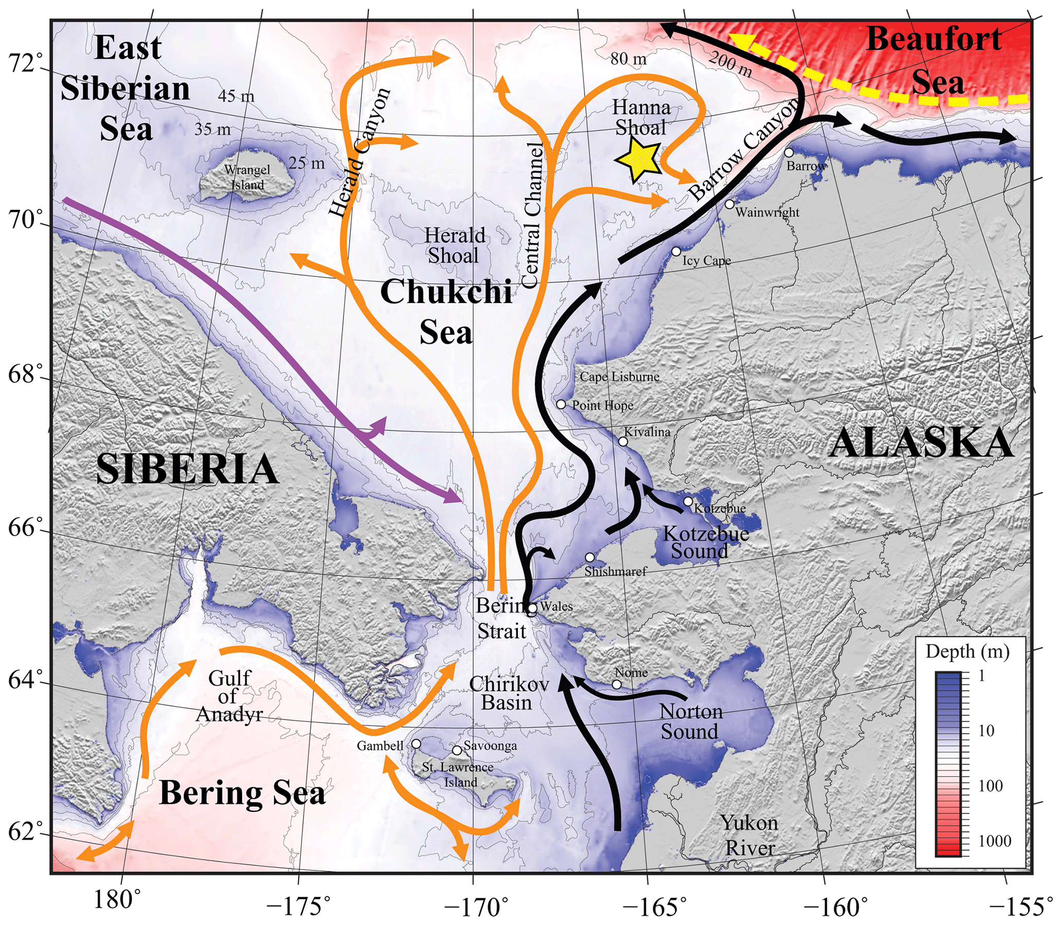
Figure 1 Map of the study area. Bathymetry of the Chukchi, northern Bering, East Siberian, and eastern Beaufort seas is shown in color. The Chukchi Ecosystem Observatory (CEO) location near Hanna Shoal is marked with a yellow star. General circulation patterns are shown with arrows: black – Alaskan Coastal Water and Alaskan Coastal Current, dividing into the Shelf-break Jet (right) and Chukchi Slope Current (left, Corlett and Pickart, 2017); orange – Anadyr, Bering, and Chukchi Seawater; purple – Siberian Coastal Current; yellow – Beaufort Gyre boundary current. Figure is from Hauri et al. (2018).

Perturbation of the seawater carbonate system associated with ocean acidification and climate change can have significant physiological and ecological consequences for marine species and ecosystems (Doney et al., 2020). All parameters of the carbonate system (pH, pCO₂, Ω_arag, concentrations of HCO${}_{\mathrm{3}}^{-}$, CO${}_{\mathrm{3}}^{\mathrm{2}-}$, etc.) have the potential to affect the physiology of marine organisms while a change in the saturation state (Ω) can lead to the dissolution of unprotected or “free” CaCO₃ structures. Recent work has highlighted the importance of local adaptation to the present environmental variability as a key factor driving species sensitivity to ocean acidification (Vargas et al., 2017, 2022). As carbonate chemistry conditions vary enormously between regions, marine organisms are naturally exposed to different selective pressures and can evolve different strategies to cope with low pH or Ω or high pCO₂. For example, the deep-sea mussel Bathymodiolus brevior living around vents at 1600 m depths is capable of precipitating calcium carbonate at pH ranging between 5.36 and 7.30 and highly undersaturated waters (Tunnicliffe et al., 2009). The response to changes in the carbonate chemistry is also modulated by other environmental drivers such as temperature or food availability (e.g., Thomsen et al., 2013; Breitberg et al., 2015). Consequently, no absolute or single threshold is expected for ocean acidification (e.g., Bednaršek et al., 2021) and a pre-requisite to assessing the impact on any biota is the monitoring at a short temporal scale to characterize the present environmental niche. When it comes to future impacts, the more intense and faster the changes associated with ocean acidification, the more adverse associated biological impacts are expected (Vargas et al., 2017, 2022). As a result, it is anticipated that Arctic marine waters that are experiencing widespread and rapid ocean acidification will potentially undergo severe negative ecosystem impacts (AMAP, 2018).

Here, we present satellite sea ice coverage data and 4 years of nearly continuous salinity, temperature, and pCO₂ data, accompanied by pH, nitrate (NO₃), dissolved oxygen (O₂), and chlorophyll fluorescence data for some of the time (Table 1, Figs. 2 and 3). We develop an empirical equation for estimating pH from moored pCO₂, temperature, and salinity and evaluate it using discrete samples collected across the Chukchi Sea, Bering Sea, and Beaufort Sea. Our time series allow us to assess the seasonal and interannual variability and controls of the inorganic carbon system in the Chukchi Sea between 2016 and 2020 and characterize the chemical conditions experienced by organisms. We discuss our observations in terms of progressing acidification and implications to organisms in the Chukchi Sea region.

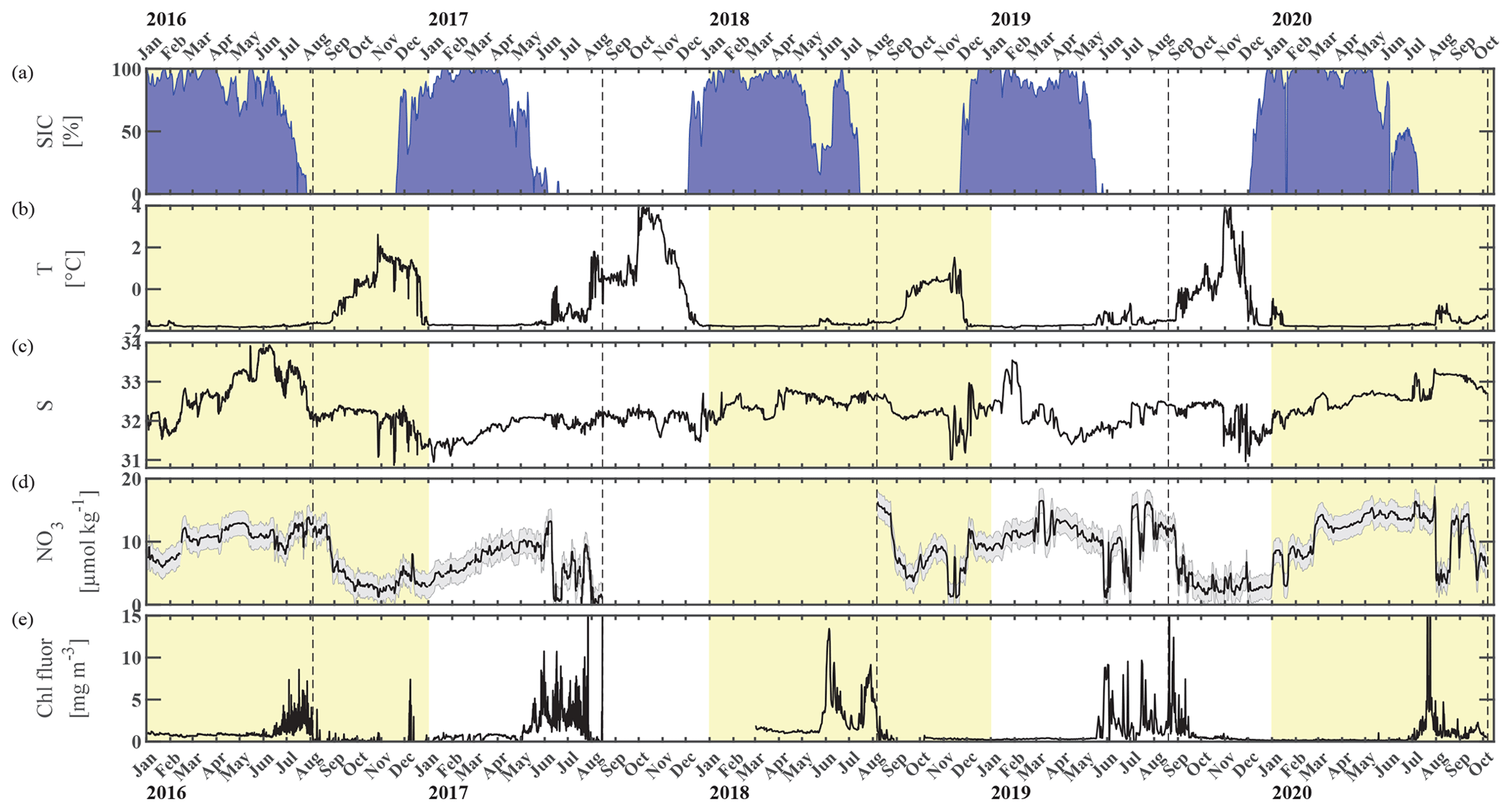
Figure 2 Chukchi Ecosystem Observatory time series from 2016 through 2020. (a) Sea ice concentration (blue shading to highlight coverage, %; DiGirolamo et al., 2022), (b) temperature (°C), (c) salinity, (d) NO₃ with uncertainty envelope (µmol kg⁻¹), and (e) chlorophyll fluorescence (mg m⁻³). Years are indicated by alternating yellow and white background shading. The vertical dashed black lines indicate the mooring turnaround timing.

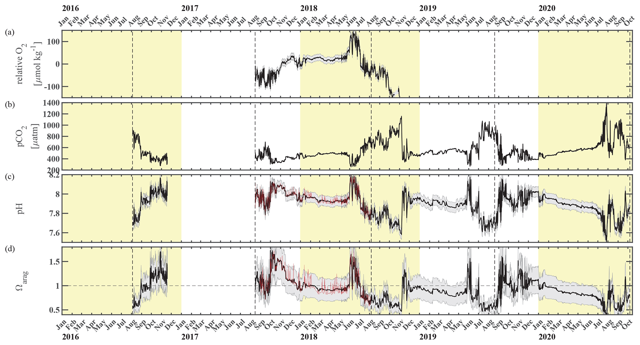
Figure 3 Chukchi Ecosystem Observatory time series from 2016 through 2020, part 2. (a) Relative dissolved oxygen with uncertainty envelope (relative to the mean; µmol kg⁻¹), (b) pCO₂ with uncertainty envelope (µatm; Hauri and Irving, 2023a), (c) pH with uncertainty envelope (pH^est in black, pH_SeaFET in red; Hauri and Irving 2023b), and (d) aragonite saturation state with uncertainty envelope (Ω_arag(pCO₂, pH^est) in black; Ω_arag(pCO₂, pH_SeaFET) in red). Years are indicated by alternating yellow and white backgrounds. The vertical dashed black lines indicate the mooring turnaround timing.

Table 1 Chukchi Ecosystem Observatory location and instrument sampling frequency. Sensor type and parameter measured (italicized) shown in top row. Values in parentheses indicate the number of measurements averaged over the measurement interval window.

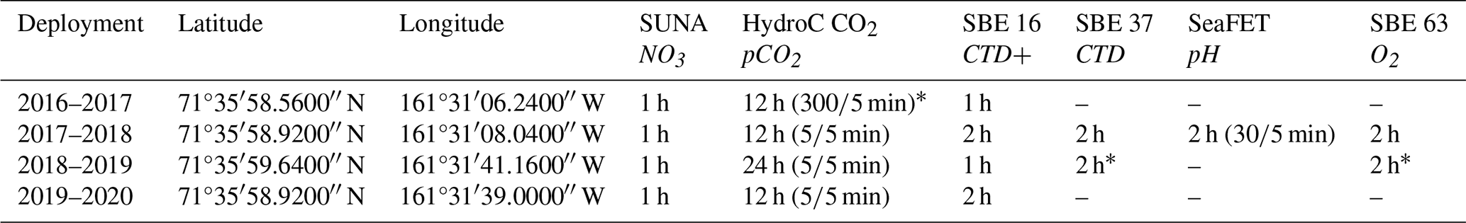
^* Indicates the sensor did not return data over the whole year due to battery failure. CTD+ indicates ancillary data was available with the SBE 16 file (e.g., chlorophyll fluorescence).

2 Materials and methods

2.1 The Chukchi Ecosystem Observatory (CEO)

The Chukchi Sea is a shallow shelf sea with maximum depths <50 m. It is largely a unidirectional inflow shelf system with Pacific origin water entering the Chukchi Sea through the Bering Strait and advecting north into the Arctic Ocean (Carmack and Wassmann, 2006). The CEO (71°36^′ N, 161°30^′ W; Fig. 1, reprinted from Hauri et al., 2018) is located along the pathway of waters flowing through Bering Strait (Fang et al., 2020) and thence from the west of Hanna Shoal toward Barrow Canyon to the south, although the wind can also drive waters from the east over the observatory site (Fang et al., 2020). From both shipboard and moored acoustic Doppler current profiler records, the south side of Hanna Shoal mean flow is characterized by a weak southward-directed current (Tian et al., 2021).

The observatory consists of oceanographic moorings that sample year-round, equipped with a variety of sensors that measure sea ice cover and thickness (Sandy et al., 2022), light, currents, waves, salinity, temperature, concentrations of dissolved oxygen, nitrate, and particulate matter, pH, pCO₂, chlorophyll fluorescence, zooplankton abundance and vertical migration (Lalande et al., 2021, 2020), the presence of Arctic cod and zooplankton (Gonzalez et al., 2021), and the vocalizations of marine mammals. During some years, the observatory included a third mooring, an experimental “freeze-up detection mooring”, which transmitted real-time data of conductivity and temperature throughout the water column until sea ice formation. The primary moorings stretch from the seafloor at 46 m to about 33 m depth, designed to avoid collisions with ice keels. Pressure sensors at the top of the moorings show less than ±1 m of excursion of the moored sensor package from its deployment mean depth in any given year, indicating that mooring blow-over or diving is not the cause of any observed large variability. Description of the CEO and lists of sensors deployed at the site can be found in Danielson et al. (2017) and Hauri et al. (2018). For this study we focus on the inorganic carbon system and its controlling mechanisms.

2.2 pCO₂

We used a CONTROS HydroC CO₂ sensor (4H-Jena Engineering GmbH, Kiel, Germany) to measure pCO₂. The CO₂ sensor was outfitted with a pump (SBE 5M, Sea-Bird Scientific) that flushes ambient seawater against a thin semi-permeable membrane, which serves as an equilibrator for dissolved CO₂ between the ambient seawater and the headspace of the sensor. Technical details about the sensor and its performance are described in Fietzek et al. (2014), who estimated sensor accuracy to be better than 1 % with post-processing.

A HydroC CO₂ sensor has been deployed at the CEO site since 2016. In all deployments, except in 2016, HydroC CO₂ sensors were post-calibrated. The lack of post-calibration in 2016 is not expected to negatively affect data quality because a battery failure resulted in data returns only over the first 3 months (August through November). Following a zero interval where the gas was pumped through a soda lime cartridge to create a zero-signal reference with respect to CO₂ and a subsequent flush interval to allow CO₂ concentrations to return to ambient conditions, measurements were taken in a burst fashion every 12 or 24 h depending on the deployment year (Table 1). Average pCO₂ values are reported as the mean of the measuring interval (Table 1) with standard uncertainty (Eq. 1) defined following best practices (Orr et al., 2018) and where the random component is the standard deviation of the mean and the systematic components include sensor accuracy and estimated error of the regression during calibration.

$$\begin{array}{}\text{(1)}& u=\sqrt{u_{\mathrm{systematic}}^{\mathrm{2}}+u_{\mathrm{random}}^{\mathrm{2}}}\end{array}$$

More than 96 % of the time, the relative uncertainty of the pCO₂ data met the weather data quality goal, defined as 2.5 % by the Global Ocean Acidification Observing Network (GOA-ON; Newton et al., 2015).

HydroC CO₂ data were processed using Jupyter Notebook scripts developed by 4H-Jena Engineering GmbH using pre- and post-calibration coefficients interpolated with any change in the zero-signal reference over the deployment (Fietzek et al., 2014). Further processing using in-house MATLAB scripts included removal of outliers, calculation of the average pCO₂, and calculation of uncertainty estimates for each measuring interval.

2.3 pH

A SeapHOx sensor (Satlantic SeaFET™ V1 pH sensor integrated with Sea-Bird Scientific SBE 37-SMP-ODO) was used to concurrently measure pH, salinity, temperature, pressure, and oxygen (Martz et al., 2010). A SeapHOx was deployed at CEO in 2016, 2017, and 2018. No SeapHOx was deployed in 2019 or 2020 due to supply chain delays and communication issues at sea. Unfortunately, measured pH (pH_SeaFET) from the 2016 and 2018 SeapHOx deployments were unusable due to high levels of noise in both the internal and external electrodes. In short, we only have usable pH data between August 2017 and August 2018.

pH_SeaFET data were excluded during a 14 d conditioning period following deployment and were processed with post-calibration corrected temperature and salinity from the SBE 37 following Bresnahan et al. (2014) using voltage from the external electrode (V_ext), and pH${}_{V_{\mathrm{ext}}}$ (pH calculated from the external electrode of the SeaFET) from an extended period of low variability (18 February 2018). Despite the availability of discrete data from one calibration cast (Cross et al., 2020b; Table 2), pH${}_{V_{\mathrm{ext}}}$ was used as the single calibration point (Bresnahan et al., 2014) for a variety of reasons: (1) there is high variability of pH_SeaFET (0.0581 pH units) straddling a 12 h window around the discrete sample collection time, (2) high temporal and spatial variability is often seen in the Chukchi Sea, and (3) the discrete pH sample was within the published SeaFET accuracy of 0.05 (Table 2, Fig. S1 in the Supplement). pH_SeaFET values are reported as the mean of the measuring interval (Table 1), and the standard uncertainty is calculated with Eq. (1) with the standard deviation of the average (random) and the SeaFET accuracy (systematic). Data handling and processing were done using in-house MATLAB scripts. pH is reported in total scale and at in situ temperature and depth for the entirety of this paper.

Table 2 Evaluation of pH_SeaFET and pH^est using reference pH from nearby discrete samples (pH${}_{\mathrm{calc}}^{\mathrm{disc}}$). Uncertainty, u_c, is the propagated combined standard uncertainty from errors.m (Orr et al., 2018). pH_SeaFET and pH^est were interpolated to the discrete timestamp. See Fig. S1 for visualization of reference values.

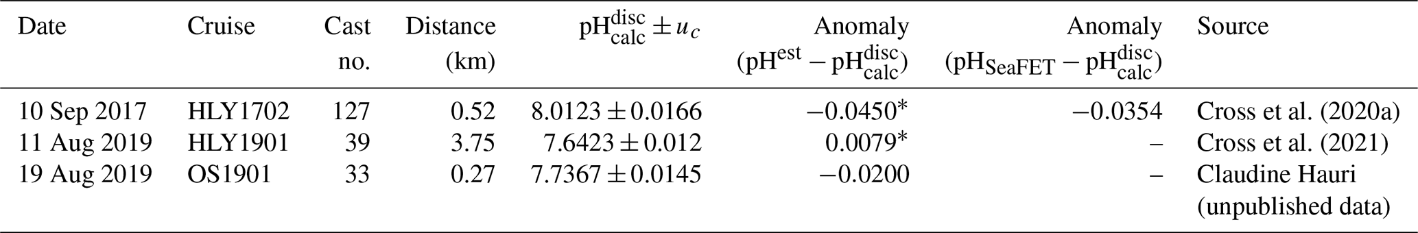
^* Indicates pH${}_{\mathrm{calc}}^{\mathrm{disc}}$ was interpolated to mooring depth.

2.4 Nitrate

NO₃ measurements were from a Submersible Ultraviolet Nitrate Analyzer (SUNA) V2 by Sea-Bird Scientific. The SUNA is an in situ ultraviolet spectrophotometer designed to measure the concentration of nitrate ions in water. SUNA V2 data were processed using a publicly available toolbox (Hennon et al., 2022; Irving, 2021) with QA/QC steps that included thermal and salinity corrections (Sakamoto et al., 2009), assessment of spectra and outlier removal based on spectral counts (Mordy et al., 2020), and concentration adjustments (absolute offset and linear drift) based on pre-deployment and post-recovery reference measurements of zero-concentration (deionized, DI) water and a nitrate standard and, when available, nutrient samples taken from Niskin bottles near the mooring site (e.g., Daniel et al., 2020).

2.5 Conductivity–temperature–depth (CTD) and oxygen instruments

Two CTDs were deployed on the CEO mooring near the HydroC CO₂ depth. The main pumped Sea-Bird SeaCAT (SBE 16) has been deployed on the CEO mooring at around 33 m depth since 2014. A pumped SBE 43 oxygen sensor was deployed with the SBE 16 during the 2015–2016, 2017–2018, and 2019–2020 deployments, but only data returns from the 2017–2018 deployment are discussed briefly in this paper (Fig. S2).

The other pumped CTD was a Sea-Bird MicroCAT (SBE 37-SMP-ODO), which was integrated with an optical dissolved oxygen sensor (SBE 63; Fig. S2), and the SeaFET pH sensor within the SeapHOx instrument. The SeapHOx was deployed in fall 2016, 2017, and 2018. The SBE 37-SMP-ODO did not record any CTD or oxygen data during the 2016 deployment and only recorded CTD and oxygen data between August and 3 November 2018 due to battery failure.

Processing of these data included temperature and conductivity correction using pre- and post-calibration data following Seabird (2016) and oxygen correction using pre- and post-calibration data following Seabird (2023). Oxygen was converted from mL L⁻¹ to µmol kg⁻¹ following Bittig et al. (2018). Density and practical salinity were calculated using the TEOS-10 GSW Oceanographic Toolbox (McDougall and Baker, 2011).

Differences between the two oxygen sensors (SBE 43 and SBE 63) of approximately 145 to 265 µmol kg⁻¹ were observed over the 2017–2018 deployment, and both moored sensors had varying offsets compared to nearby casts (Fig. S2). Therefore, only relative oxygen values from the freshly calibrated SBE 63 are discussed in this paper.

The freeze-up detection mooring (Fig. 6) consisted of four Sea-Bird SBE 37 inductive modem CTD sensors that transmitted in real time hourly temperature, salinity, and pressure data via the surface float from four subsurface depths (8, 20, 30, and 40 m; Hauri et al., 2018).

2.6 Development of empirical relationship to estimate pH

Empirical relationships for estimating water column pH have been developed for regions spanning southern, tropical, temperate, and Arctic biomes, using a variety of commonly measured parameters (e.g., pH(S, T, NO₃, O₂, Si), Carter et al., 2018; pH(O₂, T, S), Li et al., 2016; pH(θ, O₂), Watanabe et al., 2020; pH(NO₃, T, S, P) and pH(O₂, T, S, P), Williams et al., 2016; pH(O₂, T), Alin et al., 2012; pH(O₂, T) and pH(NO₃, T), Juranek et al., 2009). Given the tight coupling between the concentration of H⁺ and the concentration of the CO₂ solution, an empirical relationship for estimating surface pH from pCO₂ was developed by the National Academies of Sciences, Engineering and Medicine (2017, Appendix F). Licker et al. (2019) used this empirical relationship to calculate the global average surface ocean pH and found it represented the relationship for surface water temperatures spanning 5 to 45 °C. Here, we take a similar approach but extend it to water column pH in our cold region using temperature (T) and salinity (S) as additional proxy parameters (Eq. 2).

$$\begin{array}{}\text{(2)}& {\mathrm{pH}}^{\mathrm{est}}={\mathit{\alpha }}_{\mathrm{0}}+{\mathit{\alpha }}_{\mathrm{1}}\log \left(p{\mathrm{CO}}_{\mathrm{2}}\right)+{\mathit{\alpha }}_{\mathrm{2}}T+{\mathit{\alpha }}_{\mathrm{3}}S,\end{array}$$

where pH^est is the estimated value of water column pH, pCO₂ is from the HydroC, T and S are from the SBE 16, and all α (α₀=10.4660, ${\mathit{\alpha }}_{\mathrm{1}}=-\mathrm{0.4088}$, α₂=0.0013, ${\mathit{\alpha }}_{\mathrm{3}}=-\mathrm{0.0001}$) terms are model-estimated coefficients determined using MATLAB's multiple linear regression algorithm regress.m (Chatterjee and Hadi, 1986). After interpolating pH_SeaFET (Fig. 4, red dots) to the pCO₂ timestamp, the algorithm was trained over an arbitrarily chosen 180 d period (15 September 2017–14 March 2018, Fig. 4, dashed box). An uncertainty of 0.0525 for pH^est (Figs. 3 and S1, gray shading) was determined with Eq. (1), where the RMSE (the uncertainty in the estimation) over the entire pH_SeaFET time series is the random component and the published accuracy of the SeaFET is the systematic component (since the algorithm was trained with pH_SeaFET). The algorithm cross-validation and evaluation are discussed in Sect. 3.1. Unless explicitly defined otherwise, observations of pH refer to pH^est for the remainder of this paper.

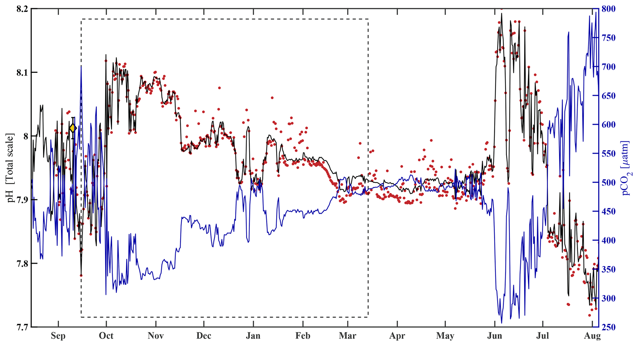
Figure 4 HydroC pCO₂ and pH highlighting mirrored trend from mid-August 2017 to beginning of August 2018. Measured pH (pH_SeaFET, red dots) is interpolated onto the HydroC pCO₂ timestamp (blue), and pH^est is shown as the solid black line. The dashed box shows the period over which pH^est was trained. The yellow diamond with error bars shows reference pH${}_{\mathrm{calc}}^{\mathrm{disc}}$ ± u_c (Table 2; Cross et al., 2020a; Orr et al., 2018).

2.7 Carbonate system calculations

Moored data were collected at different sample intervals (Table 1) and were linearly interpolated to the HydroC CO₂ timestamp to enable further calculations. TA, DIC, and Ω_arag (Figs. 11a, b and 3d) were calculated based on measured pCO₂, S, T, and pressure (P) and algorithm-based pH (pH^est). Due to a lack of data, nutrient concentrations (Si, PO₄, NH₄, H₂S) were assumed to be negligible in the CO2SYS calculations (e.g., DeGrandpre et al., 2019; Vergara-Jara et al., 2019; Islam et al., 2017). pH^est was used in lieu of pH_SeaFET to allow for calculations over the whole pCO₂ record and due to erroneously large variability of DIC and TA when pH_SeaFET was used as an input parameter (Raimondi et al., 2019; Cullison-Gray et al., 2011). The pH–pCO₂ input pair leads to large, calculated errors in DIC and TA (Raimondi et al., 2019; Cullison-Gray et al., 2011) due to strong covariance between the two parameters (both temperature and pressure dependent). Cullison-Gray et al. (2011) attributed unreasonably large short-term variability in calculated TA and DIC to temporal or spatial measurement mismatches between input pH and pCO₂ parameters and found that appropriate filtering alleviated noise spikes. By using pH^est, which by the nature of its definition is well correlated to pCO₂, we are eliminating some of these spurious noise spikes. We show Ω_arag calculated from pH_SeaFET-pCO₂ (Fig. 3d, red line) because it is less sensitive to calculated errors as it accounts for a small portion of the total CO₂ in seawater (Cullison-Gray et al., 2011).

All inorganic carbon parameters were calculated using CO2SYSv3 (Sharp et al., 2023; Lewis and Wallace, 1998) with dissociation constants for carbonic acid from Lueker et al. (2000), bisulfate from Dickson (1990), hydrofluoric acid from Perez and Fraga (1987), and the boron-to-chlorinity ratio from Lee et al. (2010). Sulpis et al. (2020) found that the carbonic-acid dissociation constants of Lueker et al. (2000) may underestimate pCO₂ in cold regions (below ∼ 8 °C) and therefore overestimate pH and CO${}_{\mathrm{3}}^{\mathrm{2}-}$. However, we choose to use Lueker et al. (2000) because they are recommended (Dickson et al., 2007; Woosley, 2021), continue to be the standard (Jiang et al., 2021; Lauvset et al., 2021), and are commonly used at high latitudes (Duke et al., 2021; Raimondi et al., 2019; Woosley et al., 2017). Furthermore, the difference between DIC calculated from pH^est and pCO₂ and discrete samples interpolated to moored instrument depth ranged from 266 to −195 µmol kg⁻¹ using the K${}_{\mathrm{1}}^{\ast }$ and K${}_{\mathrm{2}}^{\ast }$ of Sulpis et al. (2020), compared to −38 to −7 µmol kg⁻¹ using Lueker et al. (2000).

2.8 Sea ice concentration

Sea ice concentration at the observatory site was taken from the National Snow and Ice Data Center (NSIDC; DiGirolamo et al., 2022). Latitude and longitude coordinates were converted to NSIDC's EASE grid coordinate system (Brodzik and Knowles, 2002) and the 25 km gridded data were bilinearly interpolated to calculate sea ice concentration at the CEO site. Low sea ice is defined by <15 % sea ice coverage per grid cell.

2.9 Estimation of model-based ocean acidification trend

Model results were obtained from historical simulations of five different global Earth system models: (1) GFDL-CM4 (Silvers et al., 2018), (2) GFDL-ESM4 (Horowitz et al., 2018), (3) IPSL-CM6A-LR-INCA (Boucher et al., 2020), (4) CNRM-ESM2-1 (Seferian, 2019), and (5) the Max Plank Earth System Model 1.2 (MPI-ESM1-2-LR; Wieners et al., 2019) that are part of the Coupled Model Intercomparison Project Phase 6 (CMIP6). Each simulation was used to calculate the annual trend in Ω_arag and pH at the closest depth and grid cell to the CEO mooring.

3 Results

In the following, we will evaluate the pH algorithm (Sect. 3.1), analyze the large variability patterns (Sect. 3.2 and 3.3), and then take a closer look at the data from 2020 since the seasonal cycle was different in 2020 compared to previous years (Sect. 3.4).

3.1 pH algorithm

The algorithm estimated pH data from the CEO site reasonably well and within the weather uncertainty goal as defined by Newton et al. (2015) most of the time. As a first step, pH^est consistency was assessed through cross-validation (Fig. 5) using the test dataset (outside the training period; r²=0.9666, RMSE = 0.166) and across the whole time series (r²=0.9598, RMSE = 0.0161, p<0.0001; Fig. 5). Observed high-frequency spikes in pH_SeaFET (Fig. 4, red dots; Fig. 5d, red line) were not captured by the HydroC pCO₂ sensor (sampling frequency of 12 h) and, as a result, are not reproduced in the pH^est time series. Throughout the pH_SeaFET time series, pH^est overestimates pH_SeaFET by a mean of 0.0008 and median of 0.0039. Since pH^est generally overestimates pH_SeaFET, we assume that Ω_arag is also somewhat overestimated throughout this paper. Discrete water samples were used as reference values to evaluate the algorithm at the CEO site (Table 2) and were found to be within the pH^est uncertainty (Fig. S1).

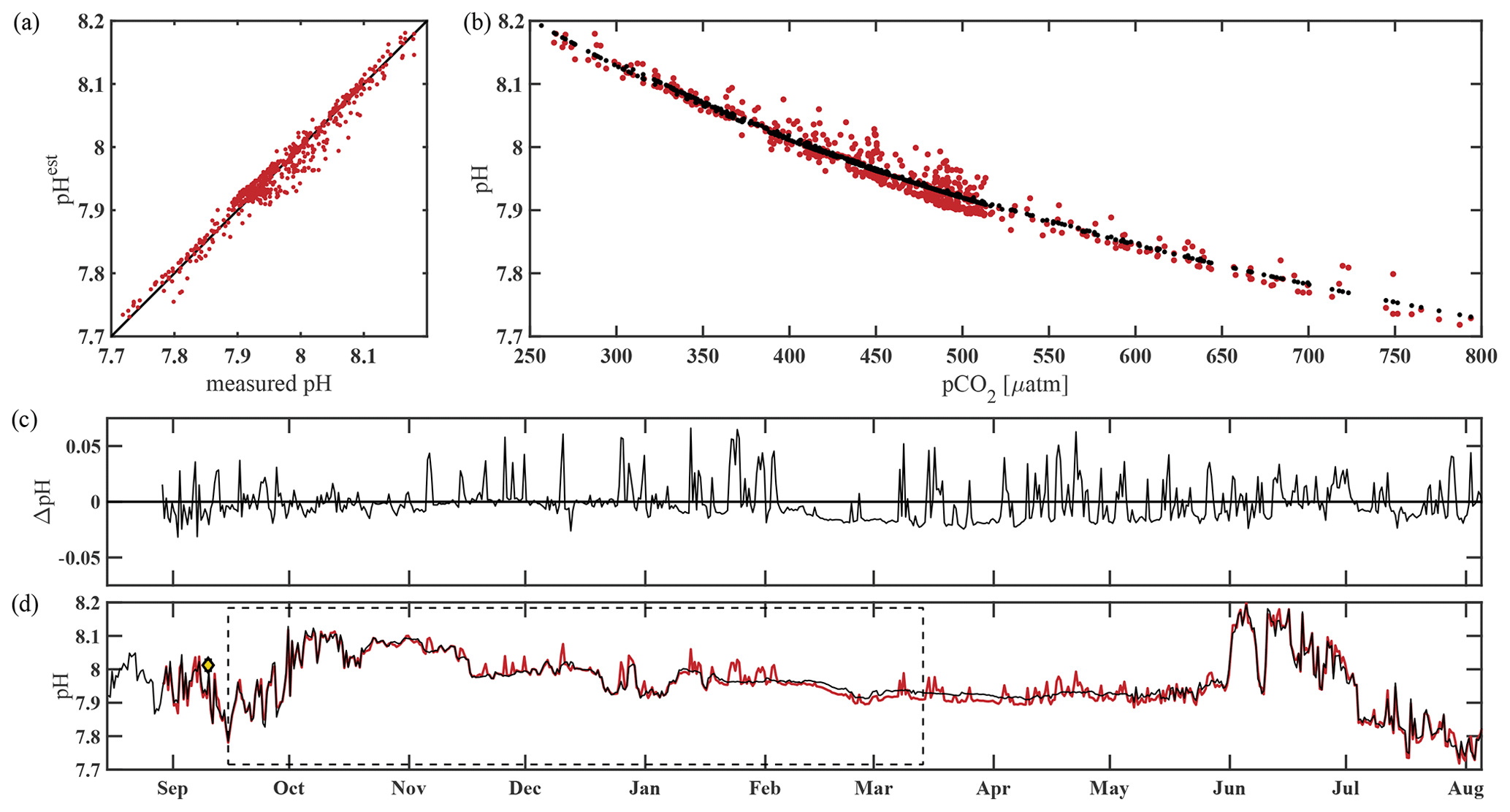
Figure 5 Performance of the pH algorithm. (a) pH_SeaFET vs. pH^est with black line highlighting 1 : 1 ratio, (b) pCO₂ vs. pH_SeaFET (red) and pCO₂ vs. pH^est (black), (c) residual pH (pH_SeaFET − pH^est), and (d) pH_SeaFET (red) and pH^est (black) vs. time, with dashed box highlighting the period over which pH^est was trained (15 September–14 March 2017) and the yellow diamond with error bars showing reference pH${}_{\mathrm{calc}}^{\mathrm{disc}}$ ± u_c (Table 2; Cross et al., 2020).

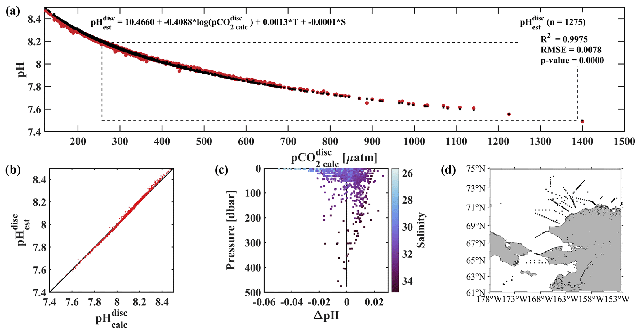
Figure 6 Evaluation of the pH algorithm. pH^est evaluation with pH${}_{\mathrm{calc}}^{\mathrm{disc}}$ from discrete samples collected during four cruises in the fall or early winter (August–November) of 2017–2020 and pH${}_{\mathrm{est}}^{\mathrm{disc}}$ from our linear regression model (Eq. 2). (a) pCO₂${}_{\mathrm{calc}}^{\mathrm{disc}}$(TA, DIC) vs. pH (red pH${}_{\mathrm{calc}}^{\mathrm{disc}}$ and black pH${}_{\mathrm{est}}^{\mathrm{disc}}$) with dashed black box showing the range of pH and pCO₂ observed at the CEO at 33 m depth, (b) pH${}_{\mathrm{calc}}^{\mathrm{disc}}$ vs. pH${}_{\mathrm{est}}^{\mathrm{disc}}$ with black 1 : 1 ratio, (c) residual pH (pH${}_{\mathrm{calc}}^{\mathrm{disc}}$ − pH${}_{\mathrm{est}}^{\mathrm{disc}}$) vs. depth with color shading by salinity and black vertical line at 0, and (d) map showing the locations of the 1275 discrete water samples used for evaluation (Monacci et al., 2022; Cross et al., 2021, 2020a, b).

An independent verification of our algorithm was done using discrete data collected from the Bering Sea to the Arctic Ocean on four research cruises in 2020, 2019, 2018, and 2017 (Fig. 6d; Monacci et al., 2022; Cross et al., 2021, 2020a, b), henceforth called the DBO dataset. Samples collected from deeper than 500 m below the surface or flagged as questionable or bad were excluded from this analysis. pH and pCO₂ were calculated from 1275 discrete samples analyzed for TA, DIC, silicate, phosphate, and ammonium (except when silicate, phosphate, and ammonium were assumed to be negligible for the 327 samples from cruise SKQ202014S; Monacci et al., 2022) using CO2SYSv3 (Sharp et al., 2023; Sect. 2.7 for details) and are referred to as pH${}_{\mathrm{calc}}^{\mathrm{disc}}$ and pCO₂${}_{\mathrm{calc}}^{\mathrm{disc}}$, respectively. pH${}_{\mathrm{est}}^{\mathrm{disc}}$ was based on discrete water samples and calculated using Eq. (2) and was fit to pH${}_{\mathrm{calc}}^{\mathrm{disc}}$ using a linear regression (r²=0.9975, RMSE = 0.0078, p value < 0.0001; Fig. 6a–c). Mean and median differences between pH${}_{\mathrm{calc}}^{\mathrm{disc}}$ and pH${}_{\mathrm{est}}^{\mathrm{disc}}$ were 0 and 0.0022, respectively, with the largest anomalies observed at lower salinities (Fig. 6c). Absolute differences between pH${}_{\mathrm{est}}^{\mathrm{disc}}$ and pH${}_{\mathrm{cal}}^{\mathrm{disc}}$ over the salinity range observed at the CEO site (30.87 to 33.93) fall within the weather data quality goal (Newton et al., 2015) 98.7 % of the time with maximum absolute differences <0.03. The uncertainty of 0.0154 for pH${}_{\mathrm{est}}^{\mathrm{disc}}$ was determined using Eq. (1), where the mean combined standard uncertainty (u_c) for pH${}_{\mathrm{calc}}^{\mathrm{disc}}$ (0.0133; Orr et al., 2018) was the systematic component, and the regression RMSE was the random component.

Empirical relationships for estimating water column pH that rely on dissolved oxygen often ignore surface waters to limit biases due to decoupling the stoichiometry of the O₂ : CO₂ relationship due to air–sea gas exchange (e.g., Juranek et al., 2011; Alin et al., 2012; Li et al., 2016). We see evidence of this bias in our algorithm at low salinity (Fig. 6c) and low pCO₂ (not shown) when compared with the DBO dataset samples collected across the Arctic and from the surface to 500 m, with pH${}_{\mathrm{est}}^{\mathrm{disc}}$ overestimating pH${}_{\mathrm{calc}}^{\mathrm{disc}}$ by a maximum of 0.049. If depth is restricted to between 30 and 500 m when evaluating the algorithm with the DBO dataset, algorithm performance improves (r²=0.9990, RMSE = 0.0055, p value < 0.0001; not shown) and the maximum pH${}_{\mathrm{est}}^{\mathrm{disc}}$ overestimates pH${}_{\mathrm{calc}}^{\mathrm{disc}}$ by 0.022.

3.2 Relaxation events

The sub-surface waters at the CEO site comprise a high-pCO₂, low-pH, and low-Ω_arag environment, with mean values of pCO${}_{\mathrm{2}}^{\mathrm{mean}}$ = 538 ± 7 µatm, pH^mean = 7.91 ± 0.05, and ${\mathrm{\Omega }}_{\mathrm{arag}}^{\mathrm{mean}}$ = 0.94 ± 0.23 across the full data record (Fig. 3b–d). In the following we will focus on spikes in high pH and Ω_arag and low pCO₂ that occur in spring (May–June) and fall (September–December); we define these spikes as relaxation events (see discussion for justification of term).

Spring. Springtime relaxation events at 33 m depth that exhibit relatively higher pH and Ω_arag and lower pCO₂ compared to the overall mean are likely consequences of photosynthetic activity during sea ice break-up (Figs. 2 and 3). In June of 2018 and 2019, near-bottom pH and Ω_arag spiked to >8.17 and >1.5, respectively, while pCO₂ dropped to <286 µatm. Ω_arag remained oversaturated and pH was greater than 8.0 for nearly all of June in 2018. In 2019, the relaxation event was less sustained, with only four short (2–6 d long) events of relatively higher pH and Ω_arag > 1 in June. In both years, chlorophyll fluorescence spiked and either O₂ increased (in 2018) or NO₃ decreased (in 2019), which are signs of photosynthetic activity and primary production.

Fall. The relaxation events in fall were characterized by large and sudden drops in pCO₂, abrupt increases in pH and Ω_arag, and considerable interannual variability in their timing. Unlike the relaxation events observed in spring, we attribute these fall relaxation events to wind-induced physical mixing. To examine the controlling mechanisms causing these abrupt relaxation events in fall, we will start with using water column salinity and temperature data from a freeze-up detection buoy (Hauri et al., 2018) that was deployed in summer 2017 approximately 1 km away from the biogeochemical mooring. The freeze-up detection mooring provided temperature and salinity measurements every 7 m throughout the water column from the time of its deployment in mid-August until freeze-up. Data from the freeze-up detection mooring suggest that warmer and fresher water from the upper water column gets periodically entrained down to the location of the biogeochemical sensor package at 33 m depth, leading to enhanced variability of density in August and September (Fig. 7). Fluctuations of the pycnocline associated with the passage of internal waves could also elevate signal variances. During this time pCO₂ often decreased to or below atmospheric levels and pH sporadically reached values >8. At the end of September, a strong mixing event (with coincident strong surface winds) homogenized the water column from the surface down to the location of the sensor package and caused a sudden temperature increase from 0.4 to 3.9 °C (Figs. 7c and 8a). At the same time, pCO₂ (Figs. 7b and 8) decreased from 590 to 308 µatm. This suggests that warm and low-CO₂ surface water mixed with CO₂-rich subsurface water and led to a sustained relaxation period that subsequently lasted until mid-November. Another mixing event further eroded the water column stratification and replaced subsurface water with colder and fresher water (ice melt) from the surface at the end of October. This second large mixing event did not lead to large changes in pCO₂, pH, and Ω_arag.

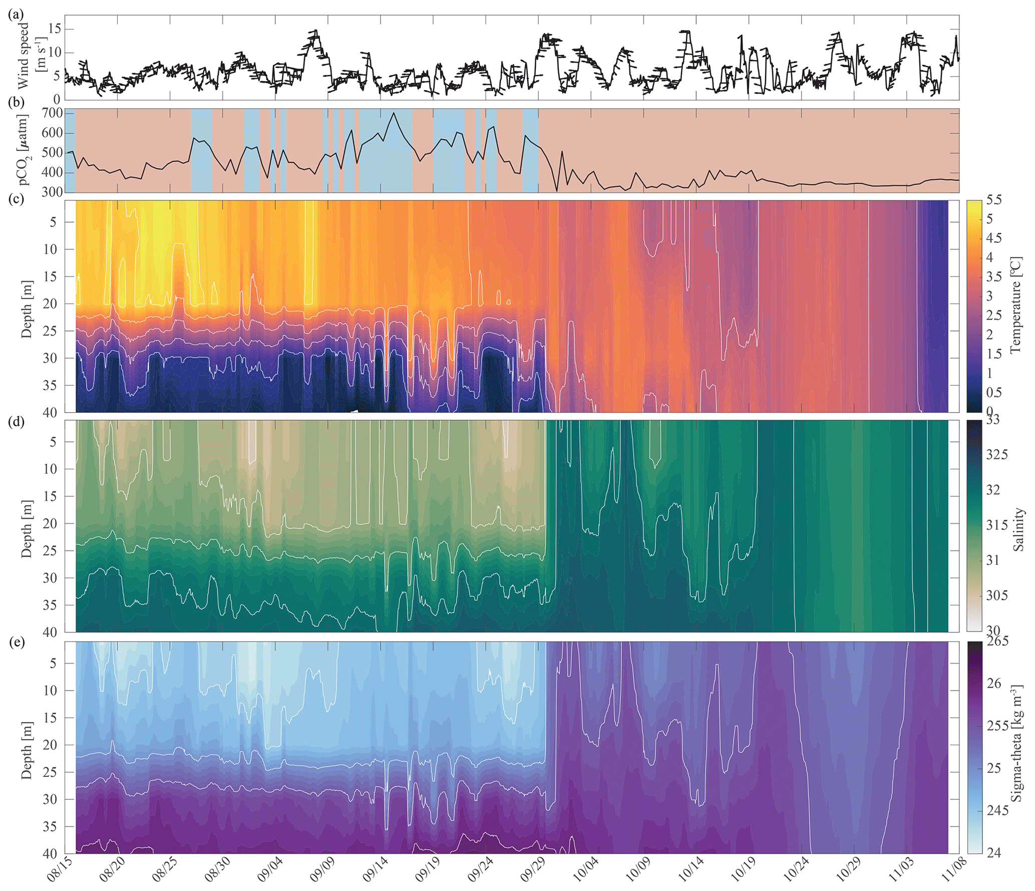
Figure 7 Water column structure from late summer 2017 to freeze-up. Profiles of (a) wind speed and direction (arrows pointing downwind) from the NOAA-operated Wiley Post–Will Rogers Memorial Airport, (b) pCO₂ (µatm) with blue background indicating the water was undersaturated regarding aragonite (Ω_arag < 1) and red shading indicating aragonite oversaturation (Ω_arag > = 1), (c) temperature (°C), (d) salinity, and (e) sigma-theta (kg m⁻³). Temperature (c) and salinity (d) were measured at 8, 20, 30, and 40 m by the Chukchi Ecosystem Observatory freeze-up detection mooring deployed in fall 2017. Density was calculated with the TEOS-10 GSW Oceanographic Toolbox (McDougall and Baker, 2011).

Salinity and temperature records from the biogeochemical mooring at 33 m depth also suggest fall season mixing events in all other years, when increases in temperature coincide with decreases in pCO₂ (Figs. 2b and c, 3a and 8). For example, two mixing events shaped the carbonate chemistry evolution in fall 2018. pCO₂ decreased from 915 µatm to around 565 µatm and Ω_arag increased to 0.9 as temperature increased and salinity decreased in early September (Figs. 2 and 8). pCO₂ then increased to 1160 µatm in late October, before decreasing to 385 µatm at the beginning of November, causing a spike in Ω_arag to 1.34. At the same time, salinity decreased by 1 unit, suggesting a strong mixing event. Throughout November 2018, pCO₂ oscillated between 344 and 757 µatm and salinity between 31.01 and 32.97, hinting at additional mixing.

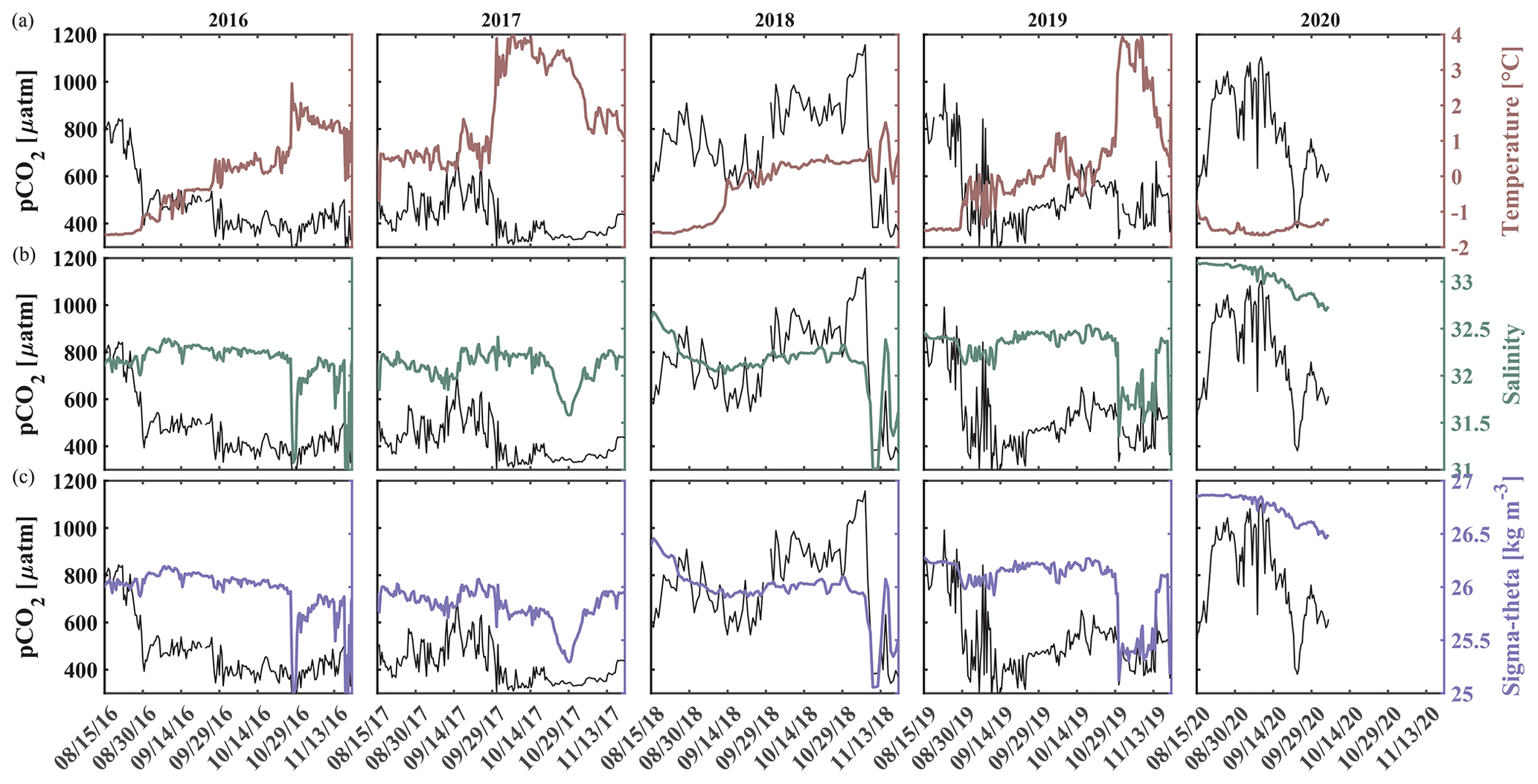
Figure 8 Impact of water column mixing on pCO₂. Time series of pCO₂ (black, left axis) and (a) temperature (maroon, right axis), (b) salinity (green, right axis), and (c) density (purple, right axis) for 15 August to 1 December in 2016–2020 measured at ∼ 33 m depth at the Chukchi Sea Ecosystem Observatory.

Similarly, an early mixing event in 2019 decreased pCO₂ to 352 µatm at the beginning of September. Short-term variability in pCO₂ with maximum levels of up to 855 µatm and minimum values below 300 µatm, variable temperature and salinity, and sporadic aragonite oversaturation events point to mixing through mid-September. At the end of October, a large mixing event homogenized the water column, accompanied by a decline in salinity by >1 unit, an increase in temperature to 4 °C, and a decrease in pCO₂ from 565 µatm to below 400 µatm. In a similar fashion to 2018, this fall mixing event was followed by a month-long period of large variability of pCO₂, salinity, pH, and Ω_arag, leading to short and sporadic aragonite oversaturation events in November and sustained oversaturation in December.

3.3 Sustained periods of low pH and Ω_arag and high pCO₂

Waters at 33 m depth at the CEO site were most acidified during the sea-ice-free periods until mixing events entrained surface waters to the sensor depth (Sect. 3.2). pH and Ω_arag started to gradually decrease from their maximum levels (Ω_{arag_max}=1.65, pH${}_{max}=\mathrm{8.19}$) at the beginning of June in 2018 to their annual low at the beginning of November (Ω_{arag_min}=0.47, pH${}_{min}=\mathrm{7.58}$; Fig. 3d and c). In November, the waters were also undersaturated with regards to calcite (not shown), and pCO₂ peaked at 1159 µatm (Fig. 3b). Dissolved oxygen decreased by about 400 µmol kg⁻¹ between July and October, when the sensor stopped working properly. The decrease in dissolved oxygen suggests remineralization of organic material. The decrease in pH, Ω_arag, and O₂ and the increase in pCO₂ was briefly interrupted by a strong mixing event in September, which entrained warmer, fresher, and CO₂-poorer water down to 33 m depth (Sect. 3.2, Fig. 8). The 2019 observations paint a similar picture of remineralization during the summer months, as the pCO₂ increase and pH and Ω_arag decreases were accompanied by an NO₃ increase (Fig. 2d and 3b–d).

pCO₂ steadily increased and pH and Ω_arag decreased during the sea-ice-covered periods (Fig. 8). pH was <8 and Ω_arag remained undersaturated under the sea ice. At the same time, NO₃ slowly increased and O₂ decreased, which points to slow organic-matter remineralization (Fig. 9). Short-term variability in pCO₂, especially in January of all three observed years, was also reflected in salinity, O₂, and NO₃ (Fig. 9) and could be attributed to advection, as the CEO site is adjacent to contrasting regimes of flow and hydrographic properties (Fang et al., 2020).

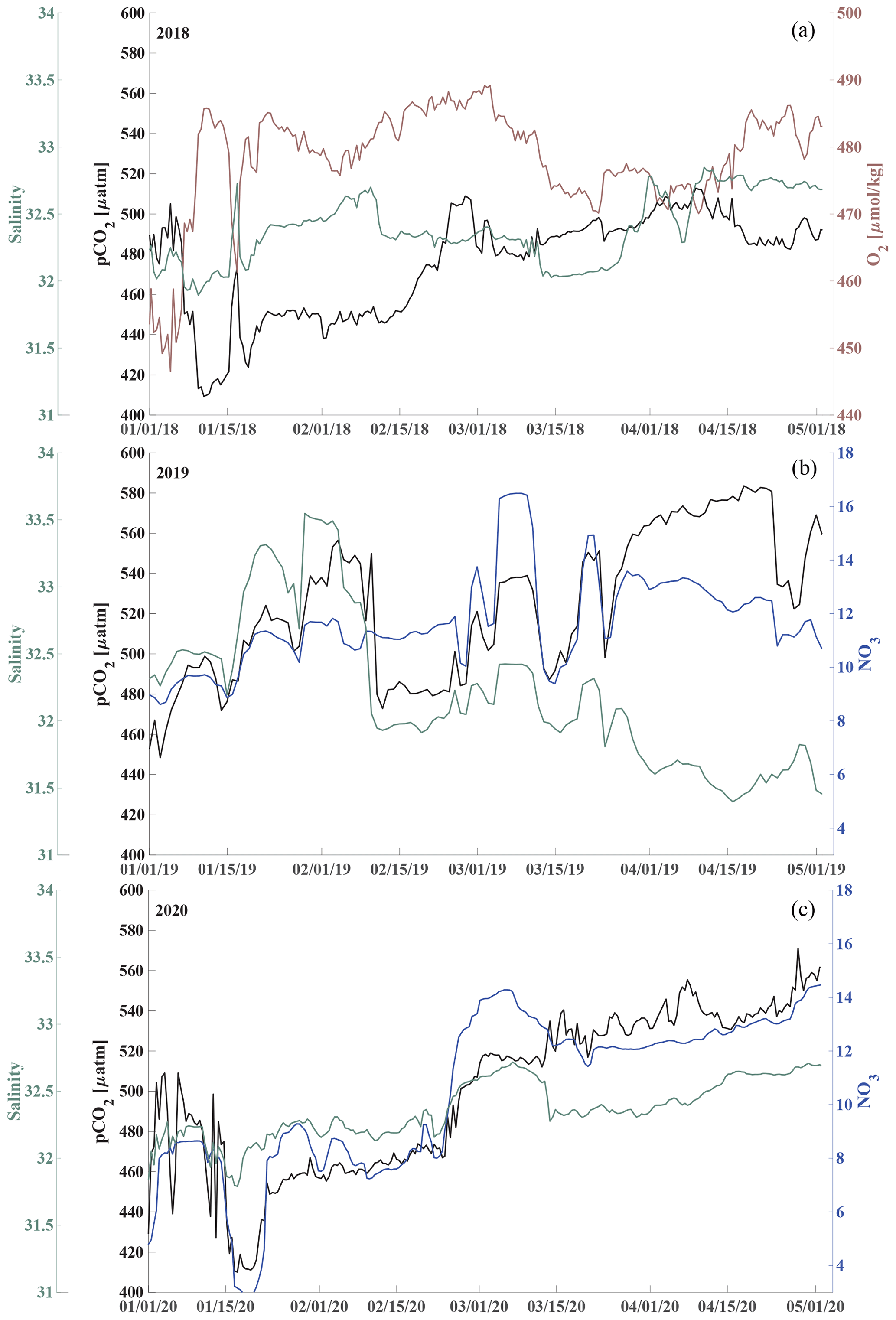
Figure 9 Respiration under the sea ice. Time series of pCO₂ (black), salinity (green, left axis), and oxygen (O₂, µmol kg⁻¹, maroon, panel a) and nitrate (NO₃, µmol kg⁻¹, blue, panels b, c) concentration (right axis during January through April for 2018, panels a, 2019 b and 2020 c).

3.4 Spring and summer of 2020 were different

The seasonal cycle in 2020 strongly contrasted with the previous observed years. pCO₂ gradually increased by roughly 200 µatm throughout the sea-ice-covered months to 650 µatm when sea ice started to retreat at the beginning of July. By the end of July, pCO₂ doubled and increased to 1389 µatm, which is the highest pCO₂ level recorded in this time series. The peak of pCO₂ was accompanied by an increase in salinity of 0.5, while temperature did not change, suggesting the influence of advection. At the beginning of August, pCO₂ dropped to 536 µatm and then oscillated around 600 µatm through much of August before returning to around 900 µatm for the next month. Similarly, pH decreased to 7.5 at the end of July and then oscillated around 7.85, while Ω_arag dropped to 0.37 and oscillated around 0.85. The steep drop and oscillation of pCO₂ was reflected in NO₃, suggesting that primary production and remineralization played a role. When pCO₂ and NO₃ decreased at the beginning of August, temperature simultaneously increased by 0.7 °C and salinity decreased by 0.12, suggesting that entrainment of shallower water masses may have played a role too. Comprehensive analyses of the factors that resulted in the 2020 differing conditions are beyond the scope of this paper but deserve attention in a future effort.

4 Discussion

CEO data provide new insights into the synoptic, seasonal, and interannual variability of the inorganic carbon system at a time when ocean acidification and climate change have already started to transform this area. The observations suggest that the CEO site is a high-CO₂ and low-pH and low-Ω_arag environment most of the time, except during sea ice break-up when the effects of photosynthetic activity remove CO₂ from the system and later in fall, when strong storm events entrain low-pCO₂ surface waters to the seafloor. Lowest pH and CaCO₃ saturation states and highest pCO₂ occur in summer through late fall when organic-matter remineralization dominates the carbonate system balance. During this time, Ω_arag can fall below 0.5 and even Ω_calc becomes sporadically undersaturated (Ω_calc<1).

4.1 pH algorithm

Deploying oceanographic equipment in remote Arctic locations is challenging. The data return from the SeapHOx sensors was disappointingly minimal, despite annual servicing and calibration by the manufacturer. Our new pH algorithm is therefore even more important as it fills pH data gaps in the CEO time series and can be applied with confidence from the Bering to the western Beaufort seas (Fig. 6). While another successful year of moored pH data return at the CEO site is needed to fully evaluate our algorithm throughout the year, comparison with single discrete water samples near the CEO site and the DBO dataset (Sect. 3.1, Table 2, Figs. 6 and S1) suggest that our algorithm-derived pH meets the weather quality uncertainty goal of ±0.02 (Newton et al., 2015) much of the time.

The combination of our new algorithm with recent progress in monitoring pCO₂ with seagliders (Hayes et al., 2022) will further increase our ability to study the inorganic carbon dynamics at times and locations when shipboard or mooring-based measurements may not be practical. Additional assessment is needed to determine to what degree the algorithm needs adjustments beyond the region evaluated in this work.

4.2 Uncertainty

Inherent spatial and temporal variability of the inorganic carbon parameters in the Chukchi Sea make the use of discrete water samples for evaluating sensor-based measurements difficult. Historic continuous surface measurements from the area suggest that surface pCO₂ can be as low as <250 µatm in early fall (Hauri et al., 2013), at a time of year when subsurface pCO₂ reaches its maximum of >800 µatm at the CEO site. This suggests a steep pCO₂ gradient of >17 µatm m⁻¹. High-resolution pH data from the 2017/2018 deployment suggests high temporal variability as well, further complicating the collection of discrete water samples to adequately evaluate the sensors. The HydroC's zeroing function, in addition to our pre- and post-calibration routines that factor into the post-processing of the data, gives us confidence in the accuracy of the pCO₂ data and further confidence in pH derived from pCO₂.

The pH^est uncertainty of 0.0525 is likely a conservative estimate based on our validation of pH^est (Sect. 3.1, Table 2). Consequently, propagated uncertainties in the calculated parameters are high. As discussed in Sect. 2.7, the pH–pCO₂ input pair exacerbates these larger uncertainties. Mean TA(pH^est, pCO₂), DIC(pH^est, pCO₂), and Ω_arag(pH^est, pCO₂) ±u_c (Orr et al., 2018) are 2173 ± 281 µmol kg⁻¹, 2111 ± 263 µmol kg⁻¹, and 0.94 ± 0.23, respectively, when input uncertainties are the standard uncertainty (Eq. 1). When the input uncertainty for pH^est is only the RMSE of 0.0161 (Sect. 3.1), uncertainties decrease to ±98 µmol kg⁻¹, ±93 µmol kg⁻¹, and ±0.09, respectively. When input uncertainties are only the random component of the input parameters (i.e., standard deviation for pH_SeaFET and pCO₂ and instrument precision for T and S), TA(pH_SeaFET, pCO₂), DIC(pH_SeaFET, pCO₂), and Ω_arag(pH_SeaFET, pCO₂) u_c drops to ±38 µmol kg⁻¹, ±37 µmol kg⁻¹, and ±0.06, respectively. Given the above uncertainties and that we do not see significant biofouling at the CEO site, we believe that short-term variability can be discussed with confidence with this dataset. In other words, wiggles in the data represent real events, despite the high uncertainty in the precise value of the calculated parameters.

4.3 Subsurface biogeochemical drivers of pH, Ω_arag, and pCO₂

Inorganic carbon chemistry can be influenced by advection and vertical entrainment of different water masses, temperature, salinity, biogeochemistry, and conservative mixing with TA and DIC freshwater endmembers. Here, we followed Rheuban et al. (2019) and separated the drivers of the observed large pH, Ω_arag, and pCO₂ variability to provide additional insights into our time series (Fig. 10) using CO2SYS by altering the input parameters temperature, salinity, TA, and DIC. Anomalies (black) relative to the reference values pH(T₀, S₀, DIC₀, TA₀), Ω_arag(T₀, S₀, DIC₀, TA₀), and pCO₂(T₀, S₀, DIC₀, TA₀) were calculated using a linear Taylor series decomposition, adding up the thermodynamic effects of temperature and salinity and the perturbations due to biogeochemistry and conservative mixing with freshwater DIC and TA endmembers (Rheuban et al., 2019). Reference values T₀, S₀, DIC₀, and TA₀, are the mean of the CEO time series. Freshwater from sea ice melt and meteoric sources (precipitation and rivers) may influence the CEO site. TA and DIC concentrations of 450 and 400 µmol kg⁻¹, respectively, have been measured in Arctic sea ice (Rysgaard et al., 2007). Riverine input along the Gulf of Alaska tends to have lower TA (366 µmol kg⁻¹) and DIC (397 µmol kg⁻¹) concentrations (Stackpoole et al., 2016, 2017) than rivers draining into the Bering, Chukchi, and Beaufort seas (TA = 1860 µmol kg⁻¹, DIC = 2010 µmol kg⁻¹; Holmes et al., 2021) all of which can influence the CEO site to some extent (Asahara et al., 2012; Jung et al., 2021). In this Taylor decomposition we used sea ice TA and DIC endmembers (Rysgaard et al., 2007) but want to emphasize that using Arctic river endmembers did not meaningfully change the results (not shown). Figure 10 shows the effects of biogeochemical processes, temperature, salinity, and conservative mixing with TA and DIC freshwater endmembers on pH, Ω_arag, and pCO₂. The effects of salinity (turquoise) and conservative mixing with TA and DIC freshwater endmembers (green) are negligible for pH, Ω_arag, and pCO₂. Temperature varied between −1.7 °C during the sea-ice-covered months and up to 4 °C in late fall, when wind events mixed the whole water column and entrained warm and low-pCO₂ surface waters to the instrument depth at 33 m (see Sect. 3.2 for a more in-depth discussion of these mixing events). During this time, the increase in temperature counteracted the effect of biogeochemistry slightly and increased pCO₂ and decreased pH (Fig. 10a, c). Temperature did not affect Ω_arag.

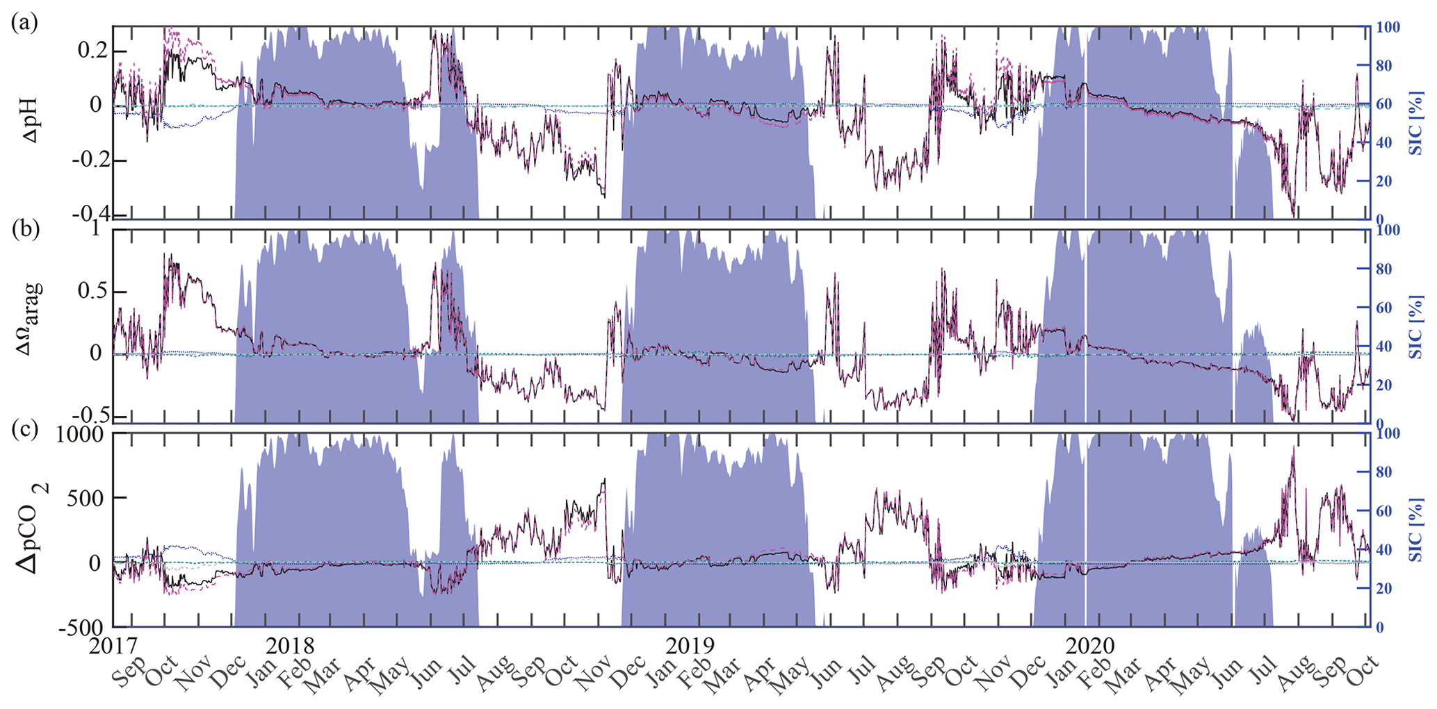
Figure 10 Drivers of the inorganic carbon system. Component time series of the linear Taylor decomposition of (a) pH, (b) Ω_arag, and (c) pCO₂. Contributions of changes in salinity (turquoise), temperature (blue), biogeochemistry (pink), and freshwater mixing (green) to changes (black, relative to the mean of the time series) in pH, Ω_arag, and pCO₂ were computed following Rheuban et al. (2019). The gray dotted line illustrates an estimated residual term. Sea ice concentration (blue shading, %; DiGirolamo et al., 2022) is shown on the right axes.

Biogeochemistry (photosynthesis, respiration, calcification, dissolution) is the most important driver of the inorganic carbon dynamics at 33 m depth at the CEO site. The springtime relaxation events in 2018 and 2019 with relatively higher pH and Ω_arag and lower pCO₂ were mainly driven by biogeochemistry (Fig. 10, magenta). During these events O₂ increased and NO₃ decreased, suggesting photosynthetic activity (Figs. 2d, e and 3a). Near-bottom photosynthetic activity by phytoplankton or sea ice algae has been observed at different locations across the Chukchi Sea (Arrigo et al., 2017; Ouyang et al., 2022; Stabeno et al., 2020; Koch et al., 2020). Sediment trap data from a CEO deployment prior to the start of this pCO₂ and pH time series suggest that export of the exclusively sympagic sea ice algae Nitzschia frigida peaked in May and June, during snowmelt and ice melt events (Lalande et al., 2020), further supporting the hypothesis that sea ice algae contributed to the CO₂ drawdown. Interestingly, TA also increased significantly during these events in 2018 and 2019, which cannot be solely attributed to organic-matter production. Specifically, TA increased by 23 µmol kg⁻¹ in 2019 (Fig. 11a). However, with an observed NO₃ decrease of 7.6 µmol kg⁻¹, we would expect an increase in TA by 7.6 µmol kg⁻¹. This is assuming that NO₃ is the primary source of nitrogen during organic-matter formation and that assimilation of 1 µmol of NO₃ leads to an increase in TA of 1 µmol (Wolf-Gladrow et al., 2007). The TA increase of 23 µmol kg⁻¹ is therefore larger than expected from organic-matter formation alone and is likely due to CaCO₃ mineral dissolution. While direct evidence is missing, the strong TA increase suggests that CaCO₃ mineral dissolution during sea ice break-up also plays an important role at the CEO site. As observed in other Arctic areas, it is possible that ikaite crystals that were trapped in the ice matrix dissolved in the water column when sea ice melted (Rysgaard et al., 2012, 2007).

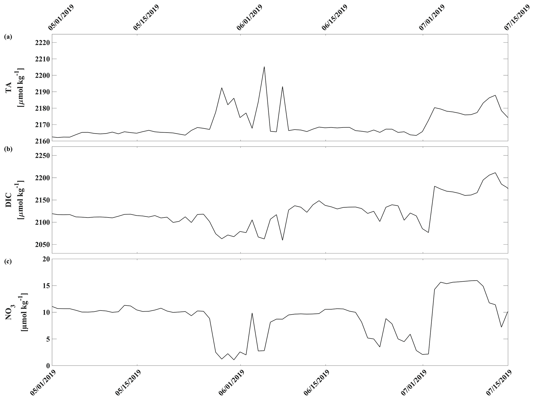
Figure 11 Spring 2019 relaxation event. Time series of (a) total alkalinity (TA, µmol kg⁻¹), (b) dissolved inorganic carbon (DIC, µmol kg⁻¹), and (c) nitrate (NO₃, µmol kg⁻¹) from 1 May through 15 July 2019.

4.4 Progression of ocean acidification in the Chukchi Sea

Organisms living at the CEO site may have always been exposed to large seasonal variability and low pH and Ω_arag (high pCO₂), but the combined and cumulative effects of climate change and ocean acidification have rapidly made these conditions more extreme and longer lasting. Ocean acidification serves as a gradual environmental press by increasing the system's mean and extreme pCO₂ and decreasing mean and extreme pH and Ω_arag. Climate-induced changes to other important controls of the inorganic carbon system, such as sea ice, riverine input, temperature, and circulation can act as sudden pulses and further modulate the inorganic carbon system to a less predictable degree and cause extreme events (Woosley and Millero, 2020; Orr et al., 2022; Hauri et al., 2021; Qi et al., 2017). Huntington et al. (2020) describe a sudden and dramatic shift of the physical, biogeochemical, and ecosystem conditions in the Chukchi and northern Bering seas in 2017. For example, satellite data for the CEO site illustrate that the longest open-water seasons on record occurred between 2017 and 2020. Before 2017, the open-water season was on average 81 (±40) d long (i.e., below 15 % concentration), of which 60 (±44) d were ice free, whereas between 2017 and 2020, the low-sea-ice period was 157 (±30) d long, of which 152 (±24) d were ice free (Fig. 12). Sea ice decline and increased nutrient influx has also promoted increased phytoplankton primary production in the area (Lewis et al., 2020; Arrigo and van Dijken, 2015; Payne et al., 2021). Since our inorganic carbon time series started after the “dramatic shift” that was observed in the Chukchi Sea in 2017 (Huntington et al., 2020) and given the uncertainty in model output in this region, we can only speculate about how the changes in sea ice, temperature, and biological production may have affected seasonal variability and extremes of the inorganic carbon chemistry at the CEO site. However, since the summertime low pH and Ω_arag and high pCO₂ are tightly coupled to the length of the ice-free period and intensity of organic-matter production, it is possible that the observed summertime period of extreme conditions may have been previously unexperienced at this site. We therefore think it is justified to call the spikes in pH and Ω_arag “ocean acidification relaxation events”, since the long-lasting summertime period of extremely low pH and Ω_arag may be a new pattern.

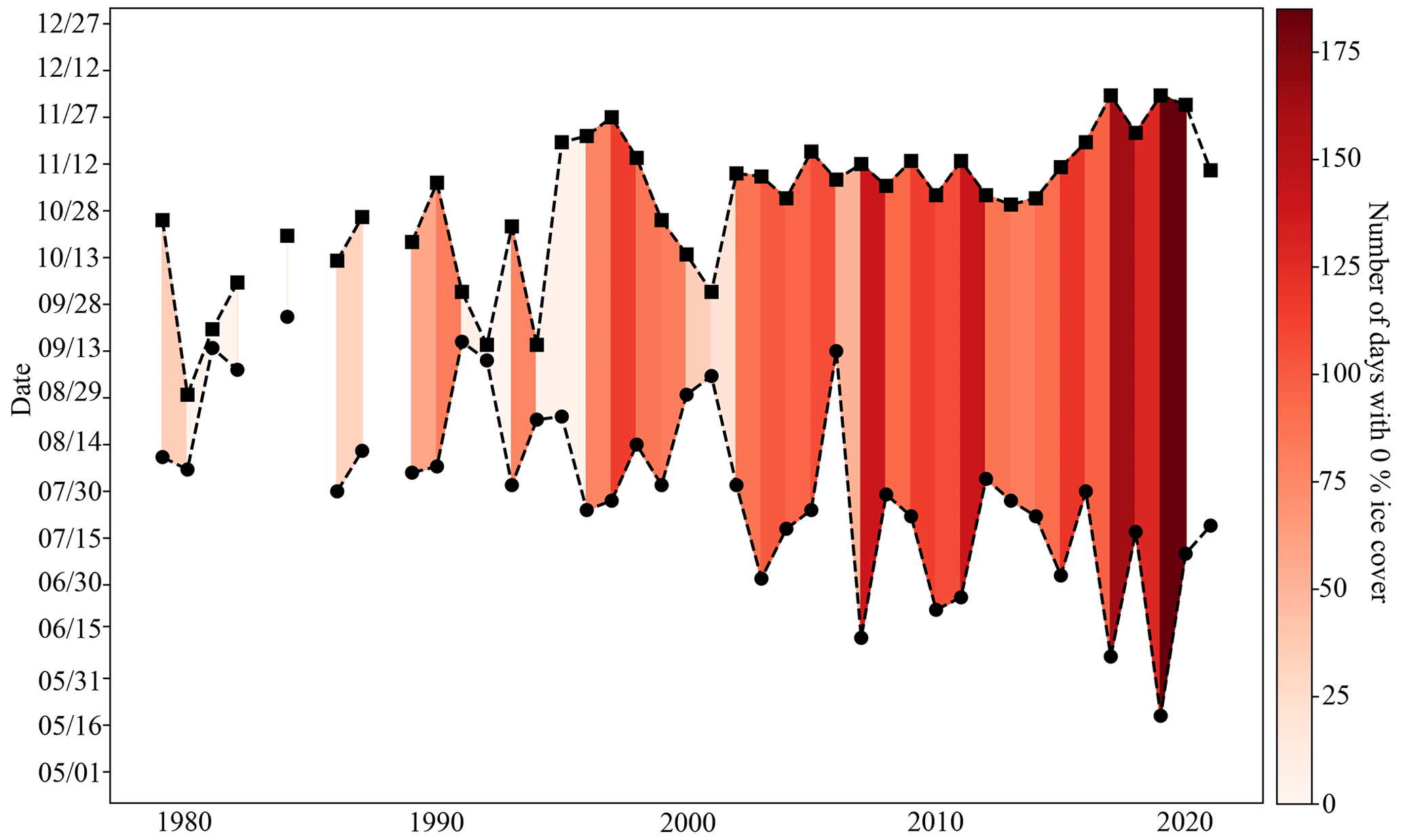
Figure 12 Low-sea-ice period at the Chukchi Sea Observatory. Time series of start (circle) and end (square) of low sea ice (<15 % per grid cell) period from 1982–2021. Shades of red illustrate the number of days with 0 % sea ice cover. The satellite sea ice cover at the observatory site was taken from the NSIDC (DiGirolamo et al., 2022).

4.5 Relevance for ecosystem

Marine organisms are exposed to a wide range of naturally fluctuating environmental conditions such as temperature, salinity, carbonate chemistry, and food concentrations that together constitute their ecological niche. As evolution works toward adaptation, the tolerance range of species and ecosystems to such parameters varies between locations and is often closely related to niche status (Vargas et al., 2022). Stress can be defined as a condition evoked in an organism by one or more environmental and biological factors that bring the organism near or over the limits of its ecological niche (after Van Straalen, 2003). The consequence of the exposure to a stressor will depend on organismal sensitivity, stress intensity (how much it deviates from present conditions), and stress duration. In a synthesis of the global literature on the biological impacts of ocean acidification, Vargas et al. (2017, 2022) showed that the extreme of the present range of variability of carbonate chemistry is a good predictor of species sensitivity. In other words, larger deviations from present extreme high pCO₂ or extreme low pH, would be expected to exert more negative biological impacts. Organismal stress and niche boundaries have implications for the definition and understanding of controls and future ocean acidification conditions in experiments aimed at evaluating future biological impacts.

Our data provide insights into conditions that affect and determine local species' ecological niches, and a necessary key is to evaluate or re-evaluate their sensitivity to present and future carbonate chemistry conditions, particularly for the sessile benthic calcifiers that constitute prey for mobile and upper trophic-level taxa. For example, an experimental study on three common Arctic bivalve species (Macoma calcarea, Astarte montagui and Astarte borealis) collected in the CEO concluded that these species were generally resilient to decreasing pH (Goethel et al., 2017). However, only two pH values were compared (a “control” (pH of 8.1) and an “acidified” treatment (pH of 7.8)) and our results show that organisms are already experiencing more extreme conditions today than have been experimentally manipulated. While these data provide insights into these species' plasticity to present pH conditions, they cannot be used to infer sensitivity to future ocean acidification or extremes of current conditions. Based on the local adaptation hypothesis (Vargas et al., 2017, 2022), stress and the associated negative effect on species fitness can be expected when pH deviates from the extreme of the present range of variability (pH < 7.5) as shown in other regions (e.g., echinoderms: Dorey et al., 2013; crustaceans: Thor and Dupont, 2015; bivalves: Ventura et al., 2016).

At the CEO, our results show sustained periods of remarkably low pH (e.g., 7.5; summer to fall, winter). Higher pH values are observed in spring and late fall. While we are lacking the local biological data to sufficiently evaluate past and future ecosystem changes, a high rate of ocean acidification as observed in the Chukchi Sea (Qi et al., 2022a, b), associated with potential temperature-induced shifts in the carbonate chemistry cycle (e.g., Orr et al., 2022), has the potential to impact species and ecosystems. Exposure to low pH increases organismal energy requirements for maintenance (e.g., acid–base regulation: Stumpp et al., 2012; compensatory calcification: Ventura et al., 2016). Organisms can cope with increased energy costs using a variety of strategies, ranging from individual physiological to behavioral responses, depending on trophic level, mobility, and other ecological factors. For example, they can use available stored energy to compensate for increased costs or they can decrease their metabolism to limit costs (AMAP, 2018). At the CEO, the low-pH period observed during the summer and fall is associated with elevated temperature and an elevated food supply for herbivores (Lalande et al., 2020). The high availability of food may then foster compensation for the higher energetic costs associated with exposure to low pH. However, a longer period of low pH as suggested by our data could lead to a mismatch between the low pH and food availability, with cascading negative consequences for the ecosystem (Kroeker et al., 2021). In winter, the low-pH conditions are associated with low temperature, no light, and low food level concentrations. These conditions are likely to keep metabolisms low and limit the negative effects of exposure to low pH (Gianguzza et al., 2014). As food availability is limited by the absence of light, this strategy may be compromised by an increase in temperature that could also lead to increased metabolism. Additional work is needed to understand the impacts of acidification conditions and variability on the marine biota of the Chukchi Sea, including field and laboratory experiments that evaluate the biological response under realistic scenarios. The characterization of the environmental conditions at the CEO, including the variability in time, can be used to design single- and multiple-stressor experiments (carbonate chemistry, temperature, salinity, food, oxygen; Boyd et al., 2018).

Indigenous communities are at the forefront of the changing Arctic, including changes in accessibility, availability, and the condition of traditional marine foods (Buschman and Sudlovenick, 2022; Hauser et al., 2021). Several marine species are critical to the food and cultural security of coastal Iñupiat, who have thrived in Arctic Alaska for millennia. While it is not possible to resolve the consequences of the seasonal and interannual variations in carbonate chemistry documented in this paper without a proper sensitivity evaluation, the seasonally low-pH conditions have the potential to impact organisms like bivalves in a foraging hotspot for walrus (Jay et al., 2012; Kuletz et al., 2015). Walrus, as well as their bivalve stomach contents, are important nutritional, spiritual, and cultural components, raising concerns for food security in the context of ecosystem shifts associated with the variability and multiplicity of climate impacts within the region (ICC, 2015).

5 Concluding thoughts

The Chukchi Sea is undergoing a rapid environmental transformation with potentially far-reaching consequences across the ecosystem. While we are lacking a long-term time series, we used this dataset to investigate the drivers of extreme pH, Ω_arag, and pCO₂ and document conditions that could affect the ecological niches of organisms, including a fast rate of ocean acidification, elongated sea-ice-free periods, increased primary productivity, and elevated temperature. While a combination of experimental and monitoring approaches is needed for an understanding of the ecological consequences of these changes, our results also highlight the urgency to mitigate CO₂ emissions and simultaneously support Indigenous-led conservation measures to safeguard an ecosystem in transition. Indigenous People in the Arctic have established strategies to monitor, adapt to, and conserve the ecosystems upon which they depend. Ethical and equitable engagement of Indigenous Knowledge and the communities at the forefront of climate impacts can help guide research and conservation action by centering local priorities and traditional practices, thereby supporting self-determination and sovereignty (Buschman and Sudlovenick, 2022).