Frost matters: incorporating late-spring frost into a dynamic vegetation model regulates regional productivity dynamics in European beech forests

Late-spring frost (LSF) is a critical factor influencing the functioning of temperate forest ecosystems. Frost damage in the form of canopy defoliation impedes the ability of trees to effectively photosynthesize, thereby reducing tree productivity. In recent decades, LSF frequency has increased across Europe, likely intensified by the effects of climate change. With increasing warming, many deciduous tree species have shifted towards earlier budburst and leaf development. The earlier start of the growing season not only facilitates forest productivity but also lengthens the period during which trees are most susceptible to LSF. Moreover, recent forest transformation efforts in Europe intended to increase forest resilience to climate change have focused on increasing the share of deciduous species in forests. To assess the ability of forests to remain productive under climate change, dynamic vegetation models (DVMs) have proven to be useful tools. Currently, however, most state-of-the-art DVMs do not model processes related to LSF and the associated impacts. Here, we present a novel LSF module for integration with the dynamic vegetation model Lund–Potsdam–Jena General Ecosystem Simulator (LPJ-GUESS). This new model implementation, termed LPJ-GUESS-FROST, provides the ability to directly attribute simulated impacts on forest productivity dynamics to LSF. We use the example of European beech, one of the dominant deciduous species in central Europe, to demonstrate the functioning of our novel LSF module. Using a network of tree-ring observations from past frost events, we show that LPJ-GUESS-FROST can reproduce productivity reductions caused by LSF. Further, to exemplify the effects of including LSF dynamics in DVMs, we run LPJ-GUESS-FROST for a study region in southern Germany for which high-resolution climate observations are available. Here, we show that modeled LSF plays a substantial role in regulating regional net primary production (NPP) and biomass dynamics, emphasizing the need for LSF to be more widely accounted for in DVMs.

1 Introduction

In temperate climates, late-spring frost (LSF) plays a critical role in the functioning of forest ecosystems (Grossman, 2023). Below-freezing temperatures during the early stages of leaf development damage photosynthetic tissue (Inouye, 2000; Chen et al., 2023), hamper secondary growth (Dittmar et al., 2006; Príncipe et al., 2017), induce mobilization of stored carbon reserves to repair damaged tissues (D'Andrea et al., 2019), and ultimately constrain the range limits of affected tree species (Körner et al., 2016; Kollas et al., 2014a). Consequently, evidence suggests that LSF substantially reduces forest ecosystem productivity (Hufkens et al., 2012).

The frequency of LSF has increased across Europe in recent decades, displaying a trend that will likely be exacerbated under a changing climate as an earlier start to the growing season leads the timing of leaf-out and periods with high likelihood of frost to increasingly coincide (Zohner et al., 2020; Ma et al., 2019). Due to increasing warming, many deciduous tree species have experienced a shift towards earlier budburst, flowering, and subsequent leaf development (Morin et al., 2009; Menzel et al., 2001). While a longer growing season facilitates forest productivity (Keenan et al., 2014; Duveneck and Thompson, 2017), it may also bear a greater risk of detrimental LSF impacts as the period in which trees are most susceptible increases (Chamberlain and Wolkovich, 2021; Ma et al., 2019; Sangüesa-Barreda et al., 2021). Thus, it is unclear to what extent climate change will alter the impact of LSF on forest ecosystem productivity.

One of the main tree species in central Europe is Fagus sylvatica (European beech), which under potential natural vegetation conditions is the dominant species across large regions of the European landscape (Bohn and Welß, 2003). Although historic land management has reduced the proportion of European beech in forests, recent management efforts have focused on re-establishing a higher share of deciduous broadleaf species, including beech (Kenk and Guehne, 2001; Schütz, 1999). These efforts aim to increase forest resilience to climate change (Yousefpour et al., 2018). In a simple twist of fate, European beech tends to be relatively susceptible to late-spring frost, which consequently co-determines its range limits across Europe (Gazol et al., 2019; Menzel et al., 2015; Kollas et al., 2014a; Bolte et al., 2009). Since beech has also been shown to be negatively impacted by drought events (Meyer et al., 2020; Dulamsuren et al., 2017; Zimmermann et al., 2015; Scharnweber et al., 2011), the success of recent forest transformation efforts hinges on the ability of beech forests to remain productive in their current distribution range under climate change.

In this context, dynamic vegetation models (DVMs) are a useful tool to assess the impact of climate change and extreme events on forest productivity (Yao et al., 2022; Medlyn et al., 2011; Gampe et al., 2021; Rammig et al., 2010). Nevertheless, most current state-of-the-art DVMs do not simulate LSF and the associated consequences, possibly overestimating the positive effects of climate change (e.g., longer growing seasons) on the carbon sequestration potential of temperate forest ecosystems (Liu et al., 2018) and underestimating detrimental effects from climate-change-related impacts on tree health and mortality. Considering forests currently account for nearly 50 % of terrestrial net primary productivity (NPP) (Bonan, 2008), the ability of vegetation modeling to assess the impact of current and future LSF on forest NPP is crucial. To bridge this gap, we present a novel late-frost module for integration with the dynamic vegetation model LPJ-GUESS (Smith et al., 2014; Hickler et al., 2012). A phenological model to predict budburst introduced by Kramer et al. (2017) forms the basis of this new model and allows us to connect the start of leaf development with the occurrence of sub-zero temperatures. This integration with LPJ-GUESS – named LPJ-GUESS-FROST – enables us to model productivity dynamics and directly attribute them to the presence (or absence) of LSF.

The new model implementation is validated against a regional tree-ring network, and subsequently, we present the effects of LSF on European beech NPP and carbon stocks, determine shifts in intra-tree carbon allocation patterns as predicted by the model, and identify regional LSF hotspots across our study region.

2 Methods

In 1953 and 2011, well-documented late-frost events occurred across large regions of Bavaria. The 1953 event was centered around the Alps and alpine foothills in southern Bavaria; the 2011 event had its epicenter in Franconia in northern Bavaria. In both cases, freezing damage was observed in European beech (Príncipe et al., 2017; Dittmar et al., 2006). We make use of these two observed events to validate our frost implementation in LPJ-GUESS-FROST and analyze the impact of LSF on European beech productivity and biomass across Bavaria.

2.1 Overview of the dynamic vegetation model LPJ-GUESS

We use LPJ-GUESS (version 4.0.1; Lindeskog et al., 2017), a well-established dynamic vegetation model designed to simulate ecosystem processes on a regional to global scale (Smith et al., 2001, 2014). Vegetation is represented by plant functional types (PFTs), which cycle through establishment, growth, competition, and mortality. Generally, a PFT groups attributes (phenology, life strategy, drought tolerance, bioclimatic limits, etc.) of multiple similar individual species and represents them through a set of parameters. In this study, we follow the commonly used parameterization of Hickler et al. (2012) developed specifically for European tree species to explicitly simulate European beech. The model is driven by gridded daily climate, soil texture, nitrogen deposition, and global atmospheric CO₂ inputs (for a more detailed description, see Sect. 2.6). Processes are modeled on a grid cell basis where the spatial resolution of the grid cells follows the spatial resolution of the climate inputs.

The processes modeled by LPJ-GUESS to simulate primary production and growth include photosynthesis and stomatal conductance based on BIOME3 (Sykes and Prentice, 1996); allocation of NPP to various compartments based on allometric constraints (Sitch et al., 2003); stochastically simulated population dynamics (Hickler et al., 2004); biomass-destroying disturbance; and nitrogen, soil, and litter processes (Smith et al., 2014). Simulated vegetation dynamics emerge from the interaction between growth and competition for resources (e.g., light, water, and nutrients). For each grid cell, multiple “replicate” patches are simulated, each of which represents a random sample of the grid cell to account for idiosyncracies in disturbance and stand development of different vegetation stands. Within each patch, a single average individual represents cohorts of individuals established in a given year, with all individuals of a given cohort sharing the same size and form as they grow.

A key process in the context of this study is summergreen-leaf phenology, which is explicitly modeled in LPJ-GUESS as a function of daily mean temperature following a generalized chilling and growing-degree-day model (Smith et al., 2001). Chill days occur when daily mean temperature falls below 5 °C and, combined with PFT-specific parameters regulating the thermal requirement for budburst (GDD_base; Eq. 1), determine the length of dormancy.

$$\begin{array}{}\text{(1)}& {\mathrm{GDD}}_{\mathrm{base}}=k_{\mathrm{chill},a}+k_{\mathrm{chill},b}\times {\mathrm{e}}^{k_{\mathrm{chill},k}\times \mathrm{chilldays}}\end{array}$$

Subsequently, when a sufficient growing-degree sum (GDD₅; Eq. 2, mean temperature (T) over 5 °C) for a given PFT has accumulated,

$$\begin{array}{}\text{(2)}& {\mathrm{GDD}}_{\mathrm{5}}=max\mathit{\{}\mathrm{0},T-\mathrm{5}\mathit{\}},\end{array}$$

leaf unfolding commences, and the phenological status (phen, Eq. 3) is updated daily as a fraction of complete canopy cover, ranging between 0 and 1, until maximum canopy cover is reached

$$\begin{array}{}\text{(3)}& \mathrm{phen}=\left\{\begin{array}{ll}\mathrm{0},& {\mathrm{GDD}}_{\mathrm{5}}\le {\mathrm{GDD}}_{\mathrm{base}}\\ \text{min}\mathit{\{}\mathrm{1},\frac{{\mathrm{GDD}}_{\mathrm{5}}-{\mathrm{GDD}}_{\mathrm{base}}}{{\mathrm{GDD}}_{\mathrm{ramp}}}\mathit{\}},& {\mathrm{GDD}}_{\mathrm{5}}>{\mathrm{GDD}}_{\mathrm{base}},\end{array}\right.\end{array}$$

where GDD_ramp is a PFT parameter.

2.2 Implementation of budburst model and late-spring frost in LPJ-GUESS

We extended the leaf phenology calculation in LPJ-GUESS by implementing a novel model simulating LSF, running in parallel to the standard LPJ-GUESS phenology module (see Fig. A2). Late-spring frost is primarily a disruption of the phenological cycle of leaf development caused by the overlap of leaf-out and a critical sub-zero leaf temperature. The standard implementation of LPJ-GUESS phenology merely calculates the fraction of complete canopy cover (see above); thus, we here used a more specific model for calculating budburst status from Kramer et al. (2017). This sequential two-stage chilling and forcing model relies on daily mean temperature to calculate the budburst status, returning 0 when budburst has not yet occurred and 1 when budburst has taken place. The first stage of the model is the chill state (S_c; Eq. 4), which determines the period of phenological rest, calculated as

$$\begin{array}{}\text{(4)}& S_{\mathrm{c}}\left(t\right)=\sum _{i=t_{\mathrm{0}}}^t{R}_{\mathrm{c}}\left(T_i\right),\end{array}$$

where t₀ is 1 November (the day on which the phenological model resets), t is the current time step (i.e., day), and T_i is the mean air temperature at time step i. R_c(T_i) is the rate of chilling as a function of the mean air temperature at time i, formulated as

$$\begin{array}{}\text{(5)}& R_{\mathrm{c}}\left(T\right)=\left\{\begin{array}{ll}\mathrm{0},& T<T_{\mathrm{c},\min }\\ \frac{T-T_{\mathrm{c},\min }}{T_{\mathrm{c},\mathrm{opt}}-T_{\mathrm{c},\min }},& T_{\mathrm{c},\min }\le T\le T_{\mathrm{c},\mathrm{opt}}\\ \frac{T-T_{\mathrm{c},\max }}{T_{\mathrm{c},\mathrm{opt}}-T_{\mathrm{c},\max }},& T_{\mathrm{c},\mathrm{opt}}\le T\le T_{\mathrm{c},\max }\\ \mathrm{0},& T>T_{\mathrm{c},\max },\end{array}\right.\end{array}$$

where T_c,min, T_c,opt, and T_c,max are the minimum, optimum, and maximum mean air temperature required to advance chilling.

Analogously, the forcing state (S_f; Eq. 6) is calculated as the running sum of the forcing rate (R_f; Eq. 7).

$$\begin{array}{}\text{(6)}& {\displaystyle }{S}_{\mathrm{f}}\left(t\right)=\sum _{i=t_{\mathrm{1}}}^t{R}_{\mathrm{f}}\left(T_i\right),\text{(7)}& {\displaystyle }{R}_{\mathrm{f}}\left(T\right)=\left\{\begin{array}{ll}\mathrm{0},& T<T_{\mathrm{f},\min }\\ \frac{\mathrm{1}}{\mathrm{1}+e^{a_{\mathrm{f}}\left(T+b_{\mathrm{f}}\right)}},& T>T_{\mathrm{f},\min },\end{array}\right.\end{array}$$

where t₁ is the time at which the chill state reaches the critical value S_c,crit (a species-specific constant derived from empirical observations determining the end of the chilling period), T_f,min is the minimum mean air temperature required for forcing, and a_f and b_f are species-specific fitted constants. Subsequently, budburst occurs (i.e., model state is 1) when the forcing state (S_f) attains a critical value S_f,crit, which, like the critical value for chilling (S_c,crit), is derived from empirical observations.

In a second step, we cross-reference the budburst status (0 or 1) with the daily minimum temperature (T_min) to determine late-frost status. When budburst has already occurred (budburst status is 1) and T_min crosses the temperature threshold T_frost, late frost occurs. Accordingly, we calculate LSF as

$$\begin{array}{}\text{(8)}& \mathrm{LSF}(\mathrm{leafout},T_{\mathrm{frost}},T_{\min })=\left\{\begin{array}{ll}\mathrm{1},& \mathrm{leafout}=\mathrm{1}\text{ and }{T}_{\min }<T_{\mathrm{frost}}\\ \mathrm{0},& \text{else}\end{array}\right..\end{array}$$

To approximate the generally localized effect of LSF, we model T_frost stochastically for each individual patch by randomly drawing from a Gaussian distribution with mean $T_{{\mathrm{frost}}_{\mathrm{\mu }}}$ and standard deviation $T_{{\mathrm{frost}}_{\mathit{\sigma }}}$ (for details, see Sect. 2.7 and Fig. A1). A full list of the parameter values for Eqs. (1)–(5) is shown in Sect. 2.7 (Table 1).

Late-frost damage is modeled as the phenology status (where 0 indicates no canopy and 1 indicates a full canopy) being reset to zero (i.e., complete removal of existing leaves), followed by a leafless period after which the phenological state continues to advance until it reaches full canopy coverage. We implemented a constant leafless period based on observations from several studies (Menzel et al., 2015; Rubio-Cuadrado et al., 2021; Nolè et al., 2018), which found that the time between frost and full development of the second cohort of leaves ranged between ∼ 40 and ∼ 80 d. Consequently, we implement a 40 d leafless period where trees have no leaves, followed by a 20 d re-greening period where phenology steadily increases to 1 (i.e., full leaf coverage).

Since we model late-frost damage stochastically (as a function of $T_{{\mathrm{frost}}_{\mathrm{\mu }}}$ and $T_{{\mathrm{frost}}_{\mathit{\sigma }}}$) for each patch, this means that any given grid cell will have late-frost damage ranging between 0 % and 100 %. For example, if none of the patches experience frost, the grid cell has 0 % frost damage. If half of the patches experience frost, the grid cell has 50 % frost damage. Through this mechanism, we approximate a continuous function for frost damage.

The additional carbon necessary to rebuild the canopy after LSF is drawn from the carbon storage pool in LPJ-GUESS-FROST. Carbon allocation in LPJ-GUESS occurs at the end of the year, by distributing the accumulated NPP to the various biomass compartments according to a set of allometric constraints. If the accumulated NPP is not sufficient to allocate enough carbon to each compartment to satisfy these constraints, additional carbon can be “borrowed” from a carbon storage pool. This pool must be refilled when enough NPP is available. The carbon lost due to LSF is calculated as the total carbon allocated to leaves for a given year multiplied by the fraction of canopy coverage at the time of LSF. At the end of the year, during allocation, this fraction of carbon is deducted from the storage pool. A portion of this is immediately “repaid”, reducing the amount of carbon available for allocation to the structural compartments. Over subsequent years, more NPP is allocated to the storage pool until it is completely refilled.

2.3 Site-level tree-ring data

To validate the results of LPJ-GUESS-FROST, we utilized a tree-ring network consisting of previously published data from 21 sites that were affected by LSF events in 1953 (Dittmar et al., 2006) and 2011 (Príncipe et al., 2017), supplemented by data from 5 sites at the epicenter of the 2011 LSF that have been newly sampled for this study. These data allowed us to retrospectively analyze the effect of LSF on productivity in European beech. Radial growth – expressed as ring width – integrates multiple signals aside from age and climate and can be used as an indicator of variation in forest productivity (Xu et al., 2017). In the aggregate, the ring width of a given year is composed of age-, size-, climate-, and disturbance-related trends and additional, often unexplained, variability (Cook, 1987). Nonetheless, ring-width data have proven a useful tool to investigate the effect of climate on tree growth (e.g., Jevšenak, 2019; Anderegg et al., 2020; Zang et al., 2014; Bhuyan et al., 2017; Wilmking et al., 2020). To isolate the climate signal, all tree-ring-width data were detrended using a cubic spline with a frequency cutoff of 0.5 at 30 years. Detrending removes age-related growth trends from tree-ring data. The residuals of the determined spline, also called ring-width indices (RWIs), consequently depict mainly climate-induced growth variations (Sullivan et al., 2016; Cook and Peters, 1997). Following detrending, the individual tree-ring series (ranging from 10 to 30 per site) were aggregated to site-level chronologies. The median, minimum, and maximum lengths of raw tree-ring chronologies are 113 years, 32 years, and 227 years, respectively. Since the climate data used to drive LPJ-GUESS and LPJ-GUESS-FROST begin in 1951, any RWI before that year were not included in subsequent analyses. Consequently, the median, minimum, and maximum lengths of the detrended ring-width chronologies used for comparison with LPJ-GUESS-(FROST) are 62 years, 33 years, and 68 years, respectively. The median, minimum, and maximum sample sizes for the site-level chronologies are 20, 10, and 30 individual tree-ring series, respectively (Fig. A3).

2.4 Forest condition monitoring data

To complement the validation of LPJ-GUESS-FROST via tree rings, we conducted an analysis of the 2011 LSF using remote-sensing data from the European Forest Condition Monitor (EFCM; Buras et al., 2021). The EFCM provides high-resolution relative measures of forest greenness based on the Terra MODIS normalized difference vegetation index (NDVI) (Buras et al., 2021). The key value used in the context of this study is the EFCM's proportional deviation from the median (PDM) metric. This metric facilitates the comparison of absolute changes in NDVI between pixels; i.e., pixels with a lower PDM can be said to display less relative greenness than pixels with a high PDM, as referenced against the long-term median (Buras et al., 2021). To quantify the impact of the LSF on 4 May 2011, we used the PDMs from 25 May. Since the EFCM provides data integrated at a 16 d interval, this ensured that the entire post-LSF response was depicted in the PDMs. PDMs from an earlier time step would have necessarily also included pre-LSF signals. Additionally, we cross-referenced the PDMs with the regions of Bavaria that experienced sufficiently negative temperatures for LSF (see Table 1) on 4 May.

2.5 Climate data

We use two separate climate datasets to force LPJ-GUESS-(FROST) for this study. To reproduce the known site-level frost events in 1953 and 2011, we used historic, thin-plate spline-interpolated daily climate station observations (mean temperature, minimum temperature, and precipitation) from the German Meteorological Service (DWD), as downloaded from the climate data center (CDC; https://www.dwd.de/DE/klimaumwelt/cdc/cdc_node.html, last access: 15 December 2023). For each day over the analyzed period (1951–2020), available observations from an average of 227 climate stations (range 182–243 stations per day) were mapped to a digital elevation model (SRTM 90; https://cgiarcsi.community/data/srtm-90m-digital-elevation-database-v4-1/, last access: 15 December 2023) with a spatial resolution of 250 m × 250 m using a 3-dimensional thin-plate spline (function TPS in the “fields” package) with longitude, latitude, and elevation as predictors for the temperature field. This was done to account for elevational effects on minimum temperatures, which are particularly important aspects when applying critical temperature thresholds for LSF mapping. Grid sizes of commonly used gridded products (e.g., 0.1°) render gridded products too coarsely in regions with a heterogeneous topography to represent small-scale variations in minimum temperature. The mean RMSE of mapped vs. observed temperatures was 0.43 ± 0.24 K (mean ± SD).

To analyze the regional variation in LSF dynamics across Bavaria, we instead used the BayObs gridded daily climate data product provided by the Bavarian Environment Agency (LfU). This dataset provides historical daily mean temperature, daily minimum temperature, and the daily precipitation sum from 1951 until 2020 on a 5 km spatial resolution for the Bavarian domain (Bayerisches Landesamt für Umwelt, 2020). We used this dataset to avoid the excessive computational load associated with running Bavaria-wide simulations at a resolution of 250 m by 250 m.

2.6 Modeling protocol

We conducted two separate simulation experiments. Firstly, to determine the ability of LPJ-GUESS-FROST to reproduce the effect of known LSF on European beech growth, we forced LPJ-GUESS and LPJ-GUESS-FROST with the historic spline-interpolated climate data for the 26 sites in our tree-ring network. Secondly, to ascertain the wider impact of and regional variation in LSF on European beech productivity and biomass dynamics, we forced LPJ-GUESS and LPJ-GUESS-FROST with the BayObs data for the entire Bavarian domain. Aside from the climate inputs, we used the same modeling protocol for both sets of simulation experiments.

To ensure that the simulated ecosystems were in near equilibrium at the start of the simulation experiment period, we spun up the model for 1000 years using recycled climate data from the first 30 years of the climate inputs. To establish a reference baseline, we used LPJ-GUESS for the spinup, that is, the version of the model without LSF. During the spinup, stochastic disturbances were turned on to facilitate a heterogenous age structure of the simulated forests. Subsequently, we used the identical post-spinup state to start the simulation experiment period (1951–2020) runs for both LPJ-GUESS and LPJ-GUESS-FROST. To isolate the effect of LSF on productivity and biomass dynamics, we switched off stochastic disturbances in the simulation experiment period. This ensured that any diverging responses in productivity were introduced only in the simulation period and allowed us to more accurately attribute the effect of LSF on these responses.

2.7 Model parameterization

We adapted the commonly used parameterization of LPJ-GUESS for the European tree species in Hickler et al. (2012) to simulate monospecific European beech stands. The central parameters for the new frost module are described in Table 1. We used 25 replicate patches and, when applicable (i.e., during spinup), a disturbance interval of 200 years.

The frost threshold, i.e., the temperature at which leaves of European beech are damaged, is a source of some uncertainty (Chen et al., 2023). Commonly, a threshold of −2.2 °C is used for the false-spring index (Schwartz, 1993; Schwartz et al., 2006; Ma et al., 2019), and remote-sensing observations have indicated significant differences in canopy greenness between frost-affected and frost-unaffected beech at a minimum temperature of −1 °C (Buras et al., 2021). Here, we conducted a sensitivity analysis to determine the frost threshold (−1.65 °C ± 0.85 °C) by varying the frost threshold and assessing at which point the simulated response no longer matched the observed RWI response (see Fig. A1 for details). Our threshold falls well within the midrange of temperatures at which significant correlations of late-spring frost severity and gross primary productivity (GPP) were found by Chen et al. (2023).

Table 1 Parameter values used for budburst and LSF determination in LPJ-GUESS-FROST. Values for budburst calculation (b) follow those published in Kramer et al. (2017). The parameter values for the frost threshold (a) were determined using a sensitivity analysis comparing LPJ-GUESS-FROST output with RWI data from our study sites (see Fig. A1 in the Supplement for details).

2.8 Model evaluation

To assess the efficacy of LPJ-GUESS-FROST at simulating LSF, we cross-referenced simulated NPP with the observed RWI. For both metrics (NPP and RWI), we computed the resistance index (R_t) introduced by Lloret et al. (2011). This index quantifies the ratio of radial growth in an event year (e.g., a frost year) to pre-disturbance growth. In this context, growth during and before a disturbance are defined as the average growth performance across a fixed time period (Lloret et al., 2011). The direct impacts of LSF dynamics are confined to a single vegetation season; consequently, we only consider growth performance in the frost year to quantify performance during disturbance. We used a 2-year pre-disturbance window – in contrast to the more commonly used 3-year window (Pretzsch et al., 2013) – since the first LSF occurred in 1953 and our climate data start in 1951. Hence, R_t in this study solely refers to the impact of LSF on growth in comparison to the 2 years preceding LSF. We assessed statistical differences in the R_t to LSF of LPJ-GUESS, LPJ-GUESS-FROST, and RWI using a pairwise Wilcoxon rank test (Bauer, 1972).

Additionally, to analyze the impact of LSF on European beech productivity across Bavaria, we calculated the loss of NPP and biomass due to LSF as the difference between the output of LPJ-GUESS and LPJ-GUESS-FROST during the post-spinup simulation period from 1951–2020.

Post-processing of model output, subsequent statistical analysis, and manuscript authoring were done in R version 4.2.1 (R Core Team, 2022) with the addition of the following packages: meta-package tidyverse (Wickham et al., 2019), dplR (Bunn et al., 2022), fields (Nychka et al., 2021) ggthemes (Arnold, 2021), here (Müller, 2020), janitor (Firke, 2021), multcompView (Graves et al., 2019), ncdf4 (Pierce, 2022), patchwork (Pedersen, 2020), RANN (Arya et al., 2019), rnaturalearth (Massicotte and South, 2023), rnaturalearthhires (South et al., 2024), terra (Hijmans, 2022), scico (Pedersen and Crameri, 2022), sf (Pebesma, 2018), and zoo (Zeileis and Grothendieck, 2005).

3 Results

3.1 Model validation

The negative impact of LSF on RWI is evident in both documented frost years. In 1953, RWI was reduced to nearly 45 % of the pre-frost period. The impact of the 2011 frost was less severe, reducing RWI to roughly 70 % of the pre-frost baseline (Fig. 1).

LPJ-GUESS simulated a slightly higher NPP in both frost years than in the pre-frost period (indicated by R_t>1 in Fig. 1), and in both 1953 and 2011 R_t from LPJ-GUESS was significantly different from RWI R_t. In contrast, LPJ-GUESS-FROST simulated a substantial reduction in NPP (R_t<1) in both years. In 2011, the impact of the LSF on productivity is of a similar magnitude in both the tree-ring data ($\stackrel{\mathrm{̃}}{R_t}=\mathrm{0.69}$) and LPJ-GUESS-FROST ($\stackrel{\mathrm{̃}}{R_t}=\mathrm{0.55}$). For the 1953 LSF, the pattern is similar. LPJ-GUESS-FROST simulates a significant NPP reduction ($\stackrel{\mathrm{̃}}{R_t}=\mathrm{0.57}$) in response to LSF, and no significant difference is seen between LPJ-GUESS-FROST and the tree-ring data ($\stackrel{\mathrm{̃}}{R_t}=\mathrm{0.45}$).

For the 2011 LSF, the remote-sensing analysis confirms the negative impact due to frost. In the areas of Bavaria that experienced temperatures below the frost threshold of −1.65 °C on 4 May, the PDMs were substantially lower than in the areas not affected by LSF (Fig. A4).

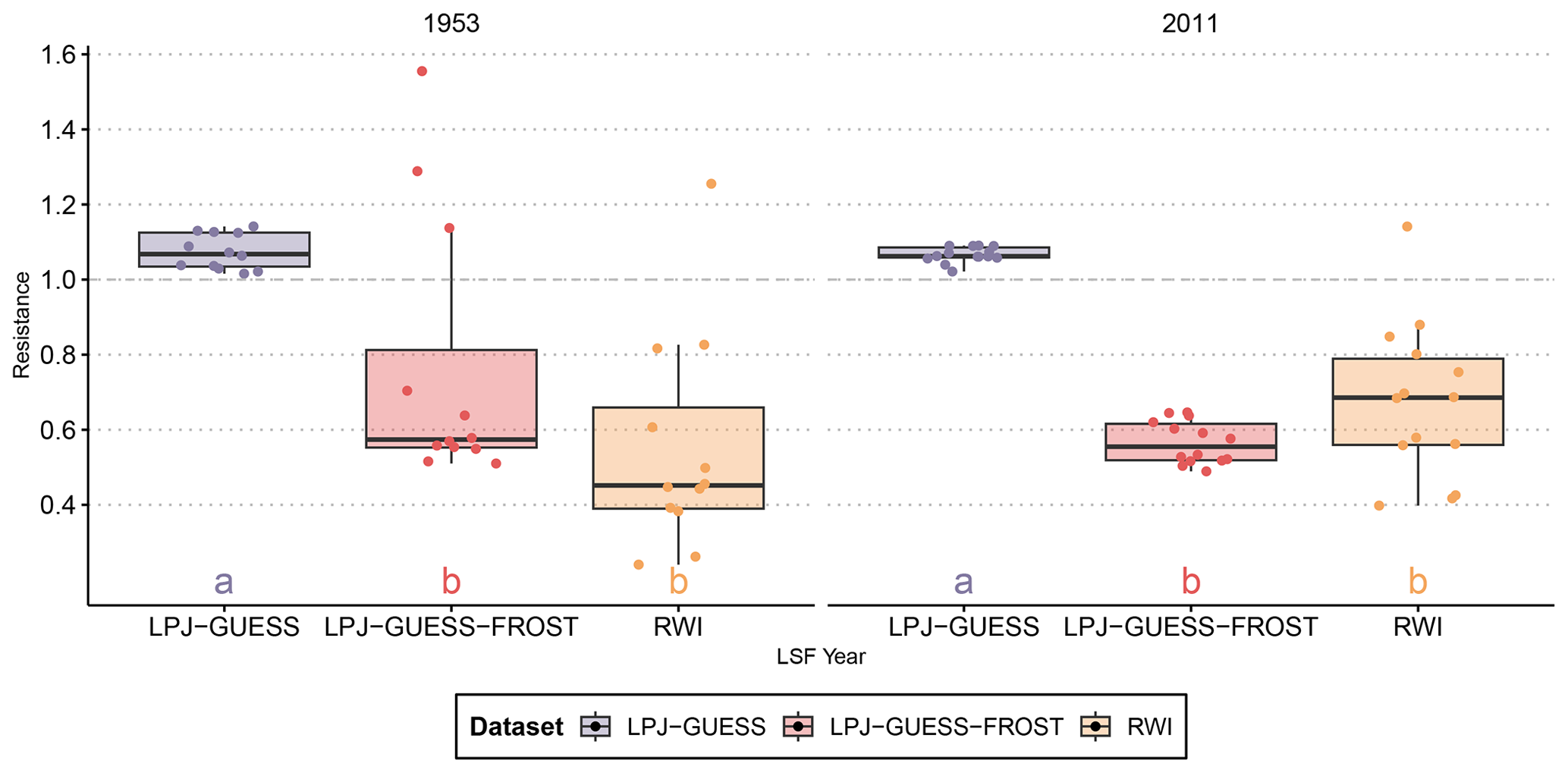
Figure 1 Resistance of observed radial growth and simulated NPP to two well-documented late-frost events. LPJ-GUESS-FROST manages to capture the late-frost signal in both cases, albeit with a larger spread in 1953. The boxplots show the median, quartiles, and 1.5 interquartile range. Lettering indicates homogenous groups based on a pairwise Wilcoxon rank sum test with Bonferroni correction for multiple testings.

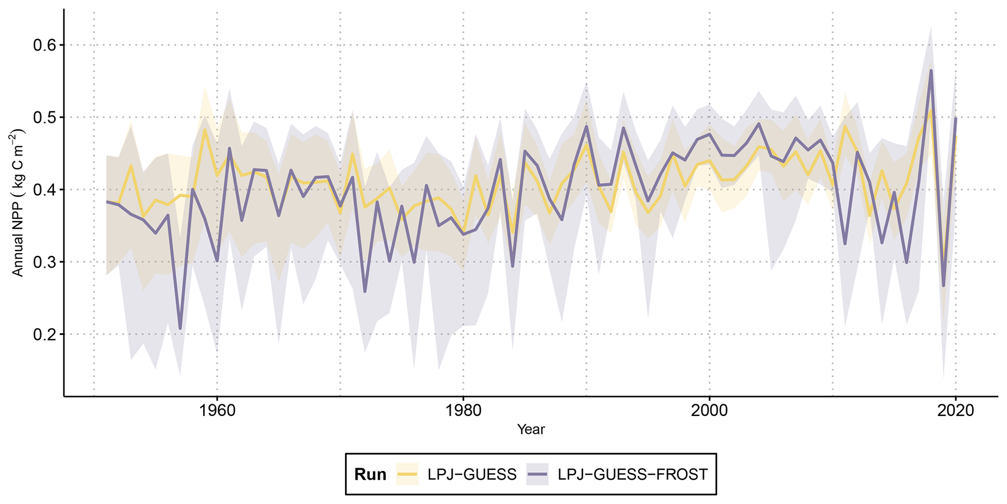
Figure 2 Time series of annual net primary productivity (NPP) from LPJ-GUESS and LPJ-GUESS-FROST. The solid lines show the mean NPP across all 2866 grid cells. The shaded areas contain the 95th percentile range of NPP. Note that due to lower NPP caused by LSF in LPJ-GUESS-FROST biomass is lower, leading to a decrease in maintenance respiration. In non-frost years, the effect of lower maintenance respiration can lead to higher NPP in LPJ-GUESS-FROST than in LPJ-GUESS.

3.2 Effects on productivity

The range of NPP across all grid cells in Bavaria varied from nearly 0.3 kg C m⁻² to around 0.6 kg C m⁻² in LPJ-GUESS. Introducing late-frost dynamics increased the variation in NPP to range from ca. 0.15 to 0.6 kg C m⁻² across all grid cells as some regions suffered from heavily decreased productivity in response to late-frost damage (Fig. 2). Simulated NPP in frost years was roughly 50 % lower than in non-frost years. Averaged across the entirety of Bavaria, the cumulative reductions in NPP caused by LSF resulted in 0.79 kg C m⁻² of lost net productivity by the end of the simulation period in 2020 (Fig. 3a).

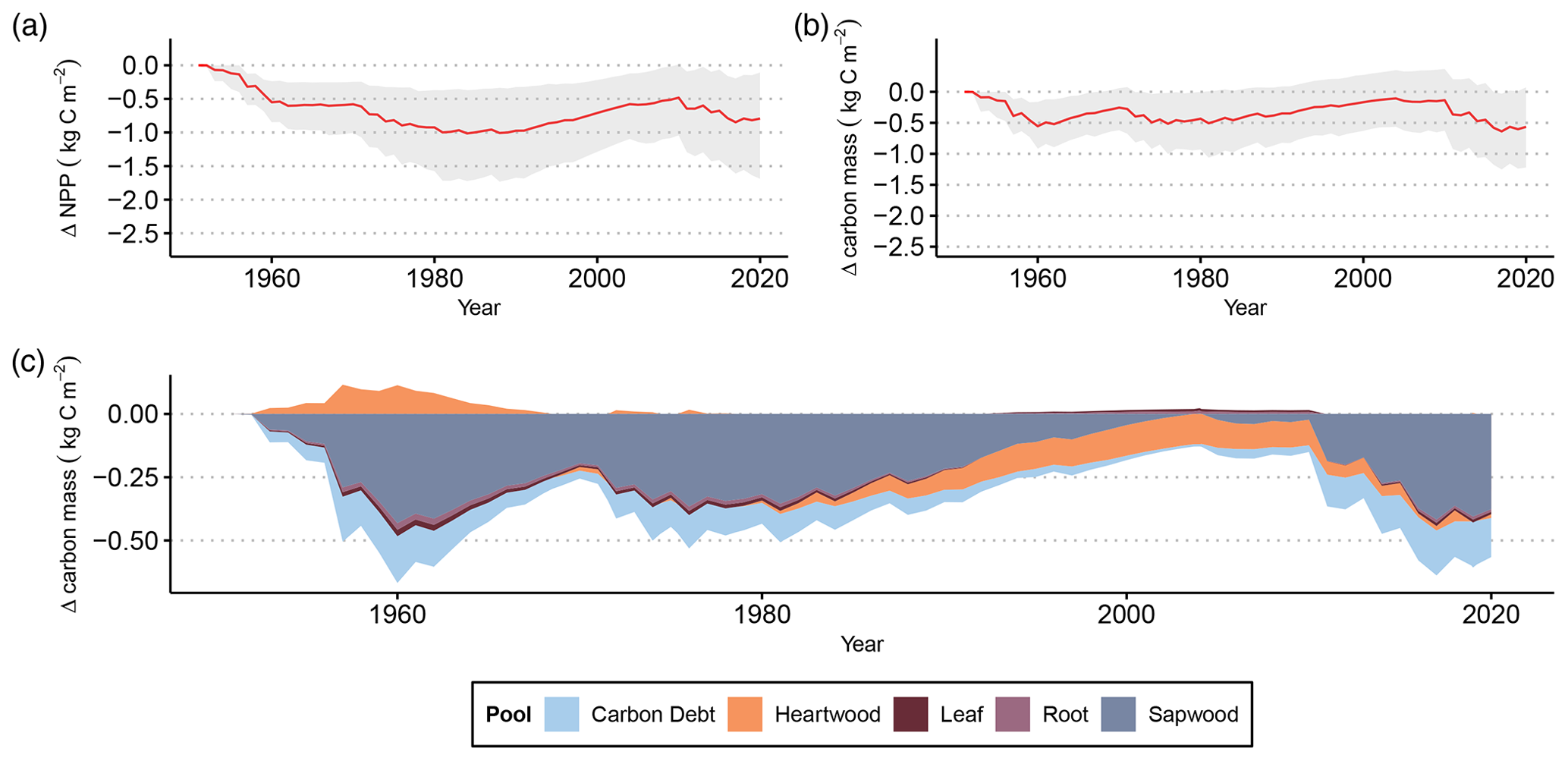
Figure 3 (a) Cumulative differences in NPP between LPJ-GUESS-FROST and LPJ-GUESS due to late-frost impacts. The red line represents the mean cumulative NPP difference across all 2866 grid cells. The shaded area contains the 95th percentile range of cumulative NPP differences. (b) Differences in total vegetation carbon biomass due to late-frost impacts. The red line shows the difference in mean carbon mass (in kg m⁻²) between LPJ-GUESS-FROST and LPJ-GUESS across all 2866 grid cells. The shaded area contains the 95th percentile range of carbon mass. (c) Depiction of each tissue pool's contribution to the total difference in vegetation carbon biomass between LPJ-GUESS-FROST and LPJ-GUESS.

The lost productivity translates to biomass loss. By 2020, the effects of LSF resulted in a mean loss of 0.57 kg m⁻² in vegetation carbon. For the 95th percentile of simulated grid cells, the change in vegetation carbon by the end of the simulation in 2020 ranges from a loss of 1.22 kg m⁻² to a gain of 0.07 kg m⁻² (Fig. 3b). This biomass loss primarily affects the sapwood, which accounts for 0.38 kg m⁻² of lost vegetation carbon by 2020 (Fig. 3c).

The modeled biomass loss is in agreement with regional altitudinal patterns across Bavaria: regional maxima of biomass loss are concentrated in low-mountain areas in the south (alpine foothills), southeast (the Bavarian Forest), and northern parts (Franconian Jura) of Bavaria (Fig. 4).

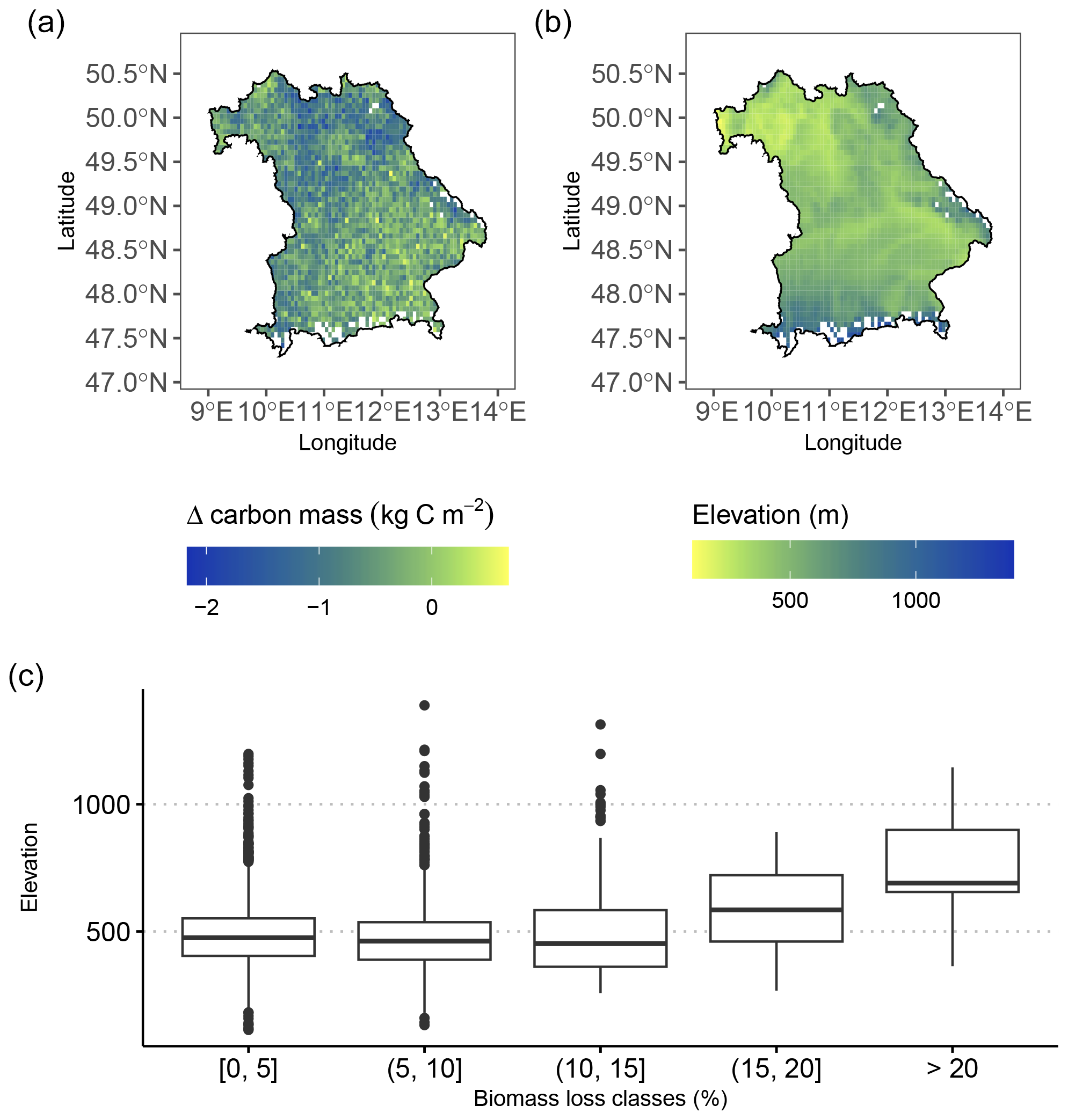
Figure 4 (a) Map showing the regional effects of late frost on whole-tree biomass loss by the end of the simulation period (2020). The heaviest losses, with up to ∼ 25 % loss of biomass due to LSF, were simulated in low-mountain regions across Bavaria (alpine foothills, the Bavarian Forest, and Franconian Jura) as indicated by (b) the elevation map (based on data from Copernicus DEM; European Space Agency, 2024). (c) The highest biomass losses (expressed in percentage of loss compared to the simulation without frost) tended to occur at higher elevations. On the contrary, low biomass losses are more evenly spread across all elevations.

4 Discussion

Using our novel implementation of late-spring frost dynamics in LPJ-GUESS (termed LPJ-GUESS-FROST), we managed to simulate the observed effect of two distinct frost events across large regions of Bavaria (Fig. 1). In both LSF years (1953 and 2011), the results from LPJ-GUESS-FROST match the RWI-based observations of variability in productivity in showing the distinct negative impact of LSF. There are no significant differences between the model and observations for both the 1953 and 2011 LSF. Notably, however, LPJ-GUESS-FROST simulates a more heterogenous frost response in 1953 than in 2011. This residual difference in the responses of LPJ-GUESS-FROST in 1953 and in 2011 can be explained by the simulated onset of budburst in those years. In 2011, the simulated onset of budburst across the 14 sites that experienced LSF ranged from day-of-year (DOY) 111 (21 April) to DOY 116 (26 April), well before LSF occurred between DOY 123 (3 May) and DOY 125 (5 May). Subsequently, from a phenological perspective, trees at all 14 sites were at risk of frost damage between DOY 123 and DOY 125. In contrast, in 1953 the simulated budburst across the 12 sites affected by LSF varied across a larger range, from DOY 117 (27 April) to DOY 142 (22 May). The recorded LSF took place between DOY 128 (8 May) and DOY 131 (11 May). At 3 sites, simulated budburst occurred after DOY 131, meaning that of the 12 sites, only 9 were phenologically predisposed to frost damage in 1953.

While the modeled responses to LSF are not significantly different from the observations, some differences remain. Discrepancies between the model output and the observational data (e.g., differences in range of modeled and observed responses in 2011) are to be expected. Firstly, we used gridded climate data to drive LPJ-GUESS-FROST, which almost certainly does not capture the actual local temperatures experienced by the sampled trees in either 1953 or 2011 as measured 2 m air temperature often deviates from canopy temperature during cold, clear nights (Kollas et al., 2014b). Secondly, while ring-width indices have been shown to be a good proxy for annual variation in NPP, some mismatch between the two metrics must be expected (Xu et al., 2017) due to differences in the demographic structure between modeled and observed tree stands. Nevertheless, our results demonstrate the efficacy of LPJ-GUESS-FROST at simulating the real-life impact of LSF on European beech productivity. Aside from reproducing the impact of the two well-known frost events for which tree-ring data were available, LPJ-GUESS-FROST simulates several additional LSF across Bavaria, suggesting that LSF is not a rare phenomenon in beech forests. Anecdotal evidence from agricultural observations confirms the occurrence of LSF in a number of the years simulated as LSF years by LPJ-GUESS-FROST (e.g., 2014, 2016, and 2019; https://www.lwg.bayern.de/weinbau/087592/index.php, last access: 15 December 2023, https://www.wetteronline.de/extremwetter/, last access: 15 December 2023).

Consequently, LPJ-GUESS-FROST enables us to show the potential extent of losses in productivity and biomass due to frost damage (Fig. 3). Frost damage consistently led to lower productivity across large regions of Bavaria. Roughly 30 % of GPP and nearly 50 % of NPP were lost to frost damage in years with late frost. This matches results from Urbanski et al. (2007), who found a severe anomaly in net ecosystem exchange (40 % of the 13-year mean) following a late-frost event in Harvard Forest in 1998. Similarly, remote-sensing analysis of an LSF event in the northeastern USA in 2010 indicated a 7 %–14 % decrease in gross ecosystem productivity due to frost damage (Hufkens et al., 2012). It is important to note that the remote-sensing approach used by Hufkens et al. (2012) necessarily includes information on all tree species in the study region. On the other hand, our simulations were specifically tailored to identify the impact of late frost on a single species, Fagus sylvatica. Therefore, a mismatch in productivity losses between the two studies is to be expected. The regional assessment done by Hufkens et al. (2012) included an early-leafing species, sugar maple, and two species with later leaf-out, American beech and yellow birch. Accordingly, sugar maples were most affected by frost damage. The lesser-affected species may in turn have buffered some of the productivity response to frost. These dynamics are absent from our study as we focused solely on simulating monospecific European beech stands. While this does not represent the current state of Bavarian forests, which until recently have been heavily managed to favor coniferous species for wood production (Kenk and Guehne, 2001; Schütz, 1999), historically, central European forests were dominated by beech (Ellenberg et al., 2010). As management efforts increasingly aim to reinstitute large shares of beech (Kenk and Guehne, 2001), our aim is to highlight the potential effect of LSF on productivity dynamics in beech forests.

Additionally, we were able to simulate the extent to which losses in primary productivity translate to losses in tree biomass (Fig. 3). The majority of simulated biomass losses stem from reduction in sapwood biomass. This behavior is consistent with observed late-frost damage in tree rings where frost-damaged trees displayed smaller sapwood increments than their non-damaged counterparts (Rubio-Cuadrado et al., 2021). Frost damage primarily manifests as a disruption of the photosynthetic apparatus via partial or full canopy defoliation (Menzel et al., 2015; Inouye, 2000). Following defoliation, affected trees must recover their canopy before full photosynthetic activity can resume, effectively shortening their growing season (Augspurger, 2009). The additive effects of a shorter growing season and reallocation of stored reserves (D'Andrea et al., 2019) to the new canopy consequently contribute to reduced radial growth in frost years. We capture part of this process by implementing a leafless period after LSF in LPJ-GUESS-FROST. After late-frost-induced canopy defoliation occurs in the model, the simulated phenology remains dormant for an extended period (see Menzel et al., 2015; Rubio-Cuadrado et al., 2021; Nolè et al., 2018). The absence of leaves in the model prohibits photosynthesis and ultimately reduces the simulated annual NPP consistent with observations.

While we are able to compare our simulated productivity losses with those estimated by Hufkens et al. (2012) and Urbanski et al. (2007), to the best of our knowledge no previous study has quantified the effect of late frost on tree biomass. This would require forest stands with identical environmental conditions aside from late frost, which is not possible in a natural setting but can be simulated using DVMs. We show that the impact of LSF on carbon storage in plant biomass in European beech forests is non-negligible. In the final year of our 69-year simulation period, the difference in vegetation carbon between LPJ-GUESS and LPJ-GUESS-FROST amounted to a 5 % reduction due to the effects of LSF. To put this in context, Lindeskog et al. (2021) found that accounting for thinning in LPJ-GUESS yielded a reduction in vegetation carbon of 3 % to 5 % across Europe until 2010 compared to a simulation without thinning, suggesting that the effect of LSF on tree biomass can have a substantial effect on forest structure and functioning.

Nevertheless, these results must be interpreted with some caution. The implementation of late-spring frost in LPJ-GUESS-FROST is intended to provide potential estimates of frost-induced shifts in carbon dynamics. In reality, LSF is a highly localized disturbance, dependent on a forest stand's microclimate and frost tolerance. Accounting for these two factors introduces stochasticity into the frost scheme of LPJ-GUESS-FROST. Currently, LPJ-GUESS-FROST cannot simulate microclimate. While replicate patches are used to abstract forest structure, this is not the case for climate, which is constant across all patches in a grid cell. In addition, the frost tolerance of European beech leaves is a point of contention. Studies directly applying freezing temperatures to twig samples have found frost tolerance for European beech to range from −4.8 to −6.4 °C at and directly following budburst (Lenz et al., 2013, 2016; Vitra et al., 2017). These results conflict with observations of frost damage in European beech stands where recorded ambient temperatures from nearby climate stations were significantly higher. In fact, frost damage in European beech has been observed at temperatures as high as −1.2 °C (Príncipe et al., 2017), and evidence from remote-sensing of LSF suggests canopy decline may already occur at −1 °C (Buras et al., 2021). Similarly, −2.2 °C is a commonly accepted species-agnostic temperature threshold for palpable frost risk (Chamberlain et al., 2019; Schwartz, 1993). This discrepancy is caused by the effect of radiative cooling. During clear windless nights, the temperature at the leaf tissue, where frost damage occurs, can potentially be several degrees lower than the ambient air temperature measured at climate stations (Matsui et al., 1981; Neuner, 2014). To overcome these problems, we inverted the mechanism determining frost occurrence. Since we cannot meaningfully model microclimate on a patch level, and there is uncertainty in the specific frost threshold of leaves, we instead decided to model the frost threshold as stochastically variable at the patch level. In this manner we approximate the local differences in frost occurrence, while simultaneously accounting for the lack of an accurate frost threshold. While this abstraction approximates the real-world heterogeneity inherent to LSF, it is stochastic in nature. Therefore, the intensity of simulated frost damage may not always match observations.

5 Conclusions and outlook

Our results indicate the importance of including late-spring frost dynamics in DVMs. We demonstrate that known patterns of productivity loss in European beech due to LSF can be reproduced by LPJ-GUESS-FROST. Additionally, we found that LSF leads to distinct regional variation in simulated biomass loss and influences the allocation of carbon within individual trees. While these findings are relevant in their own right, they also imply a need to focus future research efforts on identifying the implications of LSF across multiple tree species and climate change scenarios. To do this, further modeling efforts in the realm of LSF should attempt to simulate microclimate within stands or, at the very least, develop routines to accurately account for the discrepancy between measured 2 m air temperature and leaf temperature due to radiative cooling. Considering that commonly used forcing from general circulation model (GCM) outputs is quite coarse and therefore unlikely to capture such localized effects, this poses a particular challenge for modeling future dynamics. Additionally, due to the strong controls of leaf-out on frost risk (Vitasse et al., 2014; Ma et al., 2019), improving the phenological models used in LPJ-GUESS-FROST should be a priority. Aside from parameterizing the phenological model for a wide range of broadleaf deciduous species (maple, hornbeam, ash, etc.), future phenology routines should also consider age-dependent variation in budburst times. Similarly, while we demonstrate that accounting for loss of photosynthetic capacity due to defoliation can simulate productivity losses that are comparable to observations, the relatively simple representation of carbon costs related to LSF damage and subsequent canopy rebuilding leaves room for improvement. Here, the integration of explicitly modeled non-structural carbohydrates into LPJ-GUESS-FROST could pave the way for a better representation of LSF impacts.

Appendix A

A1 Frost threshold sensitivity analysis

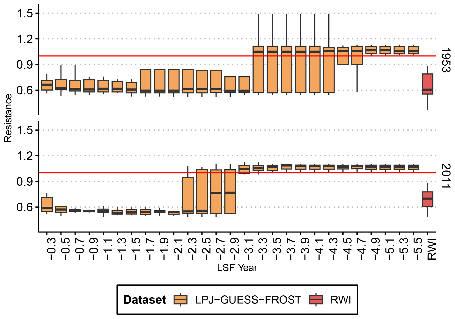
Figure A1 Sensitivity analysis to determine the range of the frost threshold. For both known frost years, we ran simulations for LPJ-GUESS-FROST with varying frost threshold temperatures from −0.3 to −5.5 °C. We then computed the resistance index (see Methods) for each simulation and for the RWI-based observations. To determine $T_{{\mathrm{frost}}_{\mathrm{\mu }}}$ and $T_{{\mathrm{frost}}_{\mathit{\sigma }}}$, we discarded all frost thresholds which resulted in a median resistance greater than 1 (i.e., higher productivity in a frost year than in pre-frost years) and computed the mean and standard deviation of the remaining thresholds (mean = −1.65; standard deviation = 0.85). The boxplots show the median resistance, quartiles, and 1.5 interquartile range. The solid red line indicates a resistance of 1.

A2 Schematic of phenology modules in LPJ-GUESS-FROST

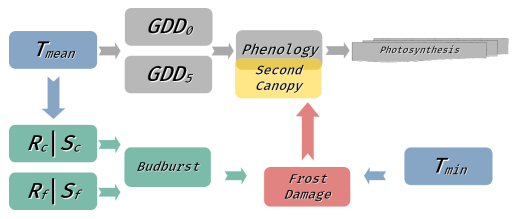
Figure A2 Schematic showing the integration of the new frost modules (red, green, and yellow) with the existing LPJ-GUESS phenology model (grey) and dependence on climatic drivers (blue). The LPJ-GUESS growing-degree day model (Eqs. 1–2 in the Methods section) simulates continuous leaf development from 0 (no leaves) to 1 (full canopy cover). This phenological status is then used for further model processes such as photosynthesis. The new frost module includes a parallel phenological budburst model which simulates a distinct point of budburst (i.e., the point at which developing leaves become sensitive to LSF). This model uses a sequential two-stage approach with a chilling stage (R_c, S_c) and a forcing stage (R_f, S_f) described in Eqs. (3)–(6) in the Methods section. This budburst status is used to determine LSF damage in conjunction with the minimum temperature (T_min). In the case of LSF, the continuous phenological status is reset to 0, and a second cohort of leaves has to be rebuilt before photosynthetic activity can resume.

A3 Site-specific tree-ring chronologies

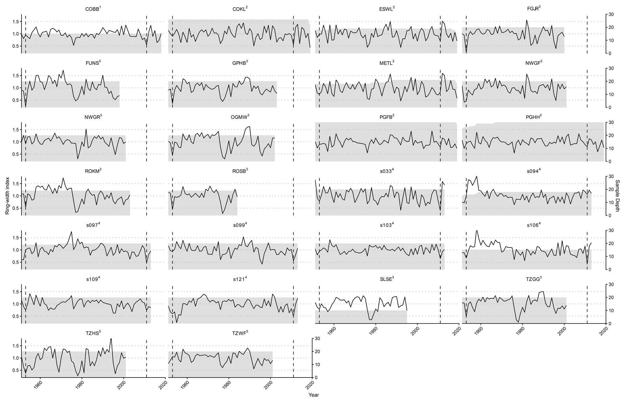
Figure A3 Spline-detrended tree-ring chronologies per site. The solid black line depicts the mean chronology of ring-width indices (left y axis), and the grey shaded area signifies the number of individual tree-ring series contained in the mean chronology in any given year (right y axis). The dashed vertical lines indicate the LSF in 1953 and 2011. Superscripts indicate the reference for each site: ¹ Meyer et al. (2020), ² Meyer (2024c), ³ Dittmar et al. (2006), and ⁴ Principe et al. (2017).

A4 Geographical extent of negative PDMs indicating LSF impacts in 2011

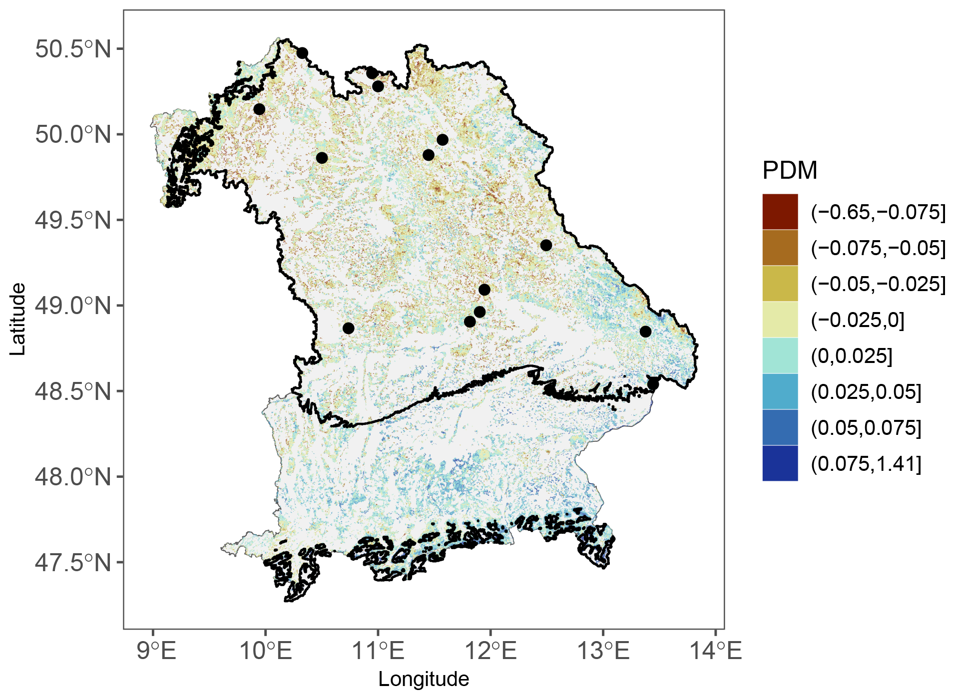
Figure A4 Map of proportional deviations from the median for the 2011 LSF from the EFCM. Black borders indicate the areas which experienced temperatures below −1.65 °C on 4 May 2011. The black dots show the tree-ring sites affected by LSF in 2011.