Seasonality and response of ocean acidification and hypoxia to major environmental anomalies in the southern Salish Sea, North America (2014–2018)

Coastal and estuarine ecosystems fringing the North Pacific Ocean are particularly vulnerable to ocean acidification, hypoxia, and intense marine heatwaves as a result of interactions among natural and anthropogenic processes. Here, we characterize variability during a seasonally resolved cruise time series (2014–2018) in the southern Salish Sea (Puget Sound, Strait of Juan de Fuca) and nearby coastal waters for select physical (temperature, T; salinity, S) and biogeochemical (oxygen, O₂; carbon dioxide fugacity, fCO₂; aragonite saturation state, Ω_arag) parameters. Medians for some parameters peaked (T, Ω_arag) in surface waters in summer, whereas others (S, O₂, fCO₂) changed progressively across spring–fall, and all parameters changed monotonically or were relatively stable at depth. Ranges varied considerably for all parameters across basins within the study region, with stratified basins consistently the most variable. Strong environmental anomalies occurred during the time series, allowing us to also qualitatively assess how these anomalies affected seasonal patterns and interannual variability. The peak temperature anomaly associated with the 2013–2016 northeast Pacific marine heatwave–El Niño event was observed in boundary waters during the October 2014 cruise, but Puget Sound cruises revealed the largest temperature increases during the 2015–2016 timeframe. The most extreme hypoxia and acidification measurements to date were recorded in Hood Canal (which consistently had the most extreme conditions) during the same period; however, they were shifted earlier in the year relative to previous events. During autumn 2017, after the heat anomaly, a distinct carbonate system anomaly with unprecedentedly low Ω_arag values and high fCO₂ values occurred in parts of the southern Salish Sea that are not normally so acidified. This novel “CO₂ storm” appears to have been driven by anomalously high river discharge earlier in 2017, which resulted in enhanced stratification and inferred primary productivity anomalies, indicated by persistently and anomalously high O₂, low fCO₂, and high chlorophyll. Unusually, this CO₂ anomaly was decoupled from O₂ dynamics compared with past Salish Sea hypoxia and acidification events. The complex interplay of weather, hydrological, and circulation anomalies revealed distinct multi-stressor scenarios that will potentially affect regional ecosystems under a changing climate. Further, the frequencies at which Salish cruise observations crossed known or preliminary species' sensitivity thresholds illustrates the relative risk landscape of temperature, hypoxia, and acidification anomalies in the southern Salish Sea in the present day, with implications for how multiple stressors may combine to present potential migration, survival, or physiological challenges to key regional species. The Salish cruise data product used in this publication is available at https://doi.org/10.25921/zgk5-ep63 (Alin et al., 2022), with an additional data product including all calculated CO₂ system parameters available at https://doi.org/10.25921/5g29-q841 (Alin et al., 2023).

1 Introduction

Northeast (NE) Pacific Ocean ecosystems are particularly vulnerable to marine heatwaves, hypoxia, and ocean acidification – the increase in seawater carbon dioxide (CO₂) due to ocean uptake of anthropogenic CO₂ emissions, which drives declining pH and calcium carbonate saturation states (Ω) – as a result of interactions among natural and anthropogenic processes. Located at the terminus of global oceanic thermohaline circulation, subsurface NE Pacific water masses have a low oxygen (O₂) and high dissolved inorganic carbon (DIC) content resulting from respiratory processes during isolation from the atmosphere (e.g., Franco et al., 2021, and references therein). Naturally high NE Pacific CO₂ levels are enhanced further through the addition of anthropogenic CO₂ (Feely et al., 2004, 2016; Sabine et al., 2004). Eastern boundary current systems accentuate this vulnerability by bringing subsurface, naturally O₂-poor, CO₂-rich waters toward the surface through upwelling (Feely et al., 2008; Chavez and Messié, 2009; Chavez et al., 2017). Estuarine systems such as the Salish Sea are typically lower in buffering capacity and are already rich in CO₂ due to dynamic local biological, hydrological, and geochemical processes; this natural estuarine acidification is amplified when oceanic waters acidified by the uptake of anthropogenic CO₂ are transported into the estuary via estuarine circulation (Feely et al., 2010, 2018; Wallace et al., 2014; Pacella et al., 2018; Cai et al., 2021; Hunt et al., 2022). Thus, estuaries connected to upwelling coastal systems, particularly in the NE Pacific, receive naturally acidified, low-oxygen marine waters relative to those in other coastal regions (e.g., Windham-Myers et al., 2018). Continually rising CO₂ emissions and other climate change effects on coastal and estuarine processes are expected to increase the spatial and temporal prevalence of acidified estuarine conditions (Pacella et al., 2018; Evans et al., 2019; Jarníková et al., 2022). Further, fjord-like estuaries with entrance sills, like Puget Sound and Hood Canal, retain some of the outgoing waters via mixing over the sills (known as reflux, e.g., MacCready et al., 2021), so anomalies tend to persist longer in these basins (Jackson et al., 2018).

Since 2007, carbonate system observations throughout the water column in coastal and estuarine NE Pacific ecosystems have proliferated, providing insight into the dynamics of ocean acidification parameters, including both measured (dissolved inorganic carbon, DIC; total alkalinity, TA; and sometimes pH on the total scale, pH_T) and calculated (pH_T; CO₂ partial pressure or fugacity, pCO₂ or fCO₂, respectively; and calcium carbonate saturation states, including aragonite, Ω_arag, and calcite, Ω_calc) variables (e.g., Feely et al., 2008, 2010; Alin et al., 2022, 2024). Hood Canal, having long been known as a hotspot for hypoxia (defined here as oxygen levels below 62 µmol kg⁻¹ = 2.0 mg L⁻¹ = 1.5 mL L⁻¹) (Newton et al., 2007), was shown to have the most severe aragonite undersaturation (Ω_arag < 1) in the southern Salish Sea during the first direct carbonate system measurements (Feely et al., 2010). Subsequent observations showed aragonite undersaturation to be prevalent throughout most of the water column, most of the time in the northern Salish Sea as well (Ianson et al., 2016; Evans et al., 2019), with numerical models showing that preindustrial Salish Sea chemistry predisposed it to rapid expansion of undersaturated conditions (Bednaršek et al., 2020a; Jarníková et al., 2022). Surface climatologies of carbonate chemistry in marine surface waters throughout Washington state revealed strong seasonal variability, with particularly high fCO₂, low pH, and low Ω values in Puget Sound surface waters during fall and winter months (November–March; Fassbender et al., 2018). Seasonal variability in pCO₂, pH, and Ω_arag observed in high-resolution moored surface time series is among the highest in the world (Sutton et al., 2016), so these waters have a long “time of emergence”, i.e., the projected time when a statistically significant anthropogenic trend in CO₂ content can be detected to emerge from the bounds of natural variability at a location (Sutton et al., 2016, 2019). Moreover, biological modulation of carbonate chemistry or temperature seasonality can obscure or decouple changes in pH and fCO₂ from those seen in saturation states (Kwiatkowski and Orr, 2018; Lowe et al., 2019; Cai et al., 2020). Estimates of anthropogenic CO₂ content from Salish Sea observations and models point to widespread Ω_arag undersaturation having emerged here and in other regional waters since preindustrial times (Feely et al., 2010; Pacella et al., 2018; Evans et al., 2019; Hare et al., 2020; Jarníková et al., 2022). These factors, in tandem with strong benthic–pelagic coupling of biogeochemical cycles (e.g., high surface productivity contributing to deep respiration hotspots; Hickey and Banas, 2008; Siedlecki et al., 2015), highlight the need for detailed biogeochemical observations throughout the water column in this biologically productive region to understand the atmospheric, terrestrial, and marine processes driving dynamic biogeochemical conditions in the Salish Sea.

Here, we use the Salish cruise data product (2008–2018; Alin et al., 2022, 2023, 2024) to characterize seasonal variability and major anomalies in physical and biogeochemical conditions in Puget Sound and its boundary waters (Strait of Juan de Fuca, coastal waters) during the seasonally resolved part of the time series (2014–2018). All calculated marine inorganic carbon parameters used in this analysis were calculated from measured dissolved inorganic carbon, total alkalinity, and ancillary hydrographic observations (temperature, salinity, and phosphate and silicate content) described by Alin et al. (2024). We used temperature, salinity, oxygen (O₂), fugacity of carbon dioxide (fCO₂), and aragonite saturation state (Ω_arag) median conditions and variation to characterize seasonal ocean acidification, hypoxia, and warming conditions across Puget Sound basins and its boundary waters. Major anomalies in large-scale marine and atmospheric temperature, as well as regional precipitation and river runoff, occurred during 2013–2018, and we qualitatively relate the timing and magnitude of observed biogeochemical anomalies in the study region to anomalies in regional weather and physical oceanography sometimes driven by these major large-scale anomalies. Cruises prior to the onset of the 2013–2018 anomalies and existing regional climatologies provided the long-term context for the apparent magnitude and duration of physical and biogeochemical anomalies observed during the seasonal sampling period. Finally, we evaluated how the physical and biogeochemical Salish cruise time series through 2018 reveals the changing landscape of multiple interacting ocean stressors as they are relevant to key ecologically and economically important fish and invertebrate species in this oceanographically dynamic region.

2 Environmental context for the Salish Sea cruise time series

Puget Sound (PS) is the southernmost glacial fjord estuarine system on the North American Pacific Coast and comprises the southern part of the Salish Sea, which also encompasses the Strait of Juan de Fuca (SJdF) and the Strait of Georgia (Fig. 1). Oceanographic conditions within PS are determined by a combination of river inputs, marine source waters, vigorous tidal mixing, bathymetric complexity, and local- to large-scale climatic influences (Moore et al., 2008; Feely et al., 2010; Banas et al., 2015; MacCready et al., 2021). PS is comprised of four basins: Main Basin (MB), South Sound (SS), Whidbey Basin (WB), and Hood Canal (HC). PS receives direct freshwater input from 14 major and many smaller rivers, draining into PS; indirect freshwater input from the Fraser River, which drains into the Strait of Georgia; and carbon and nutrient inputs from urban and agricultural environments surrounding the Salish Sea ecosystem (Mohamedali et al., 2011; Banas et al., 2015).

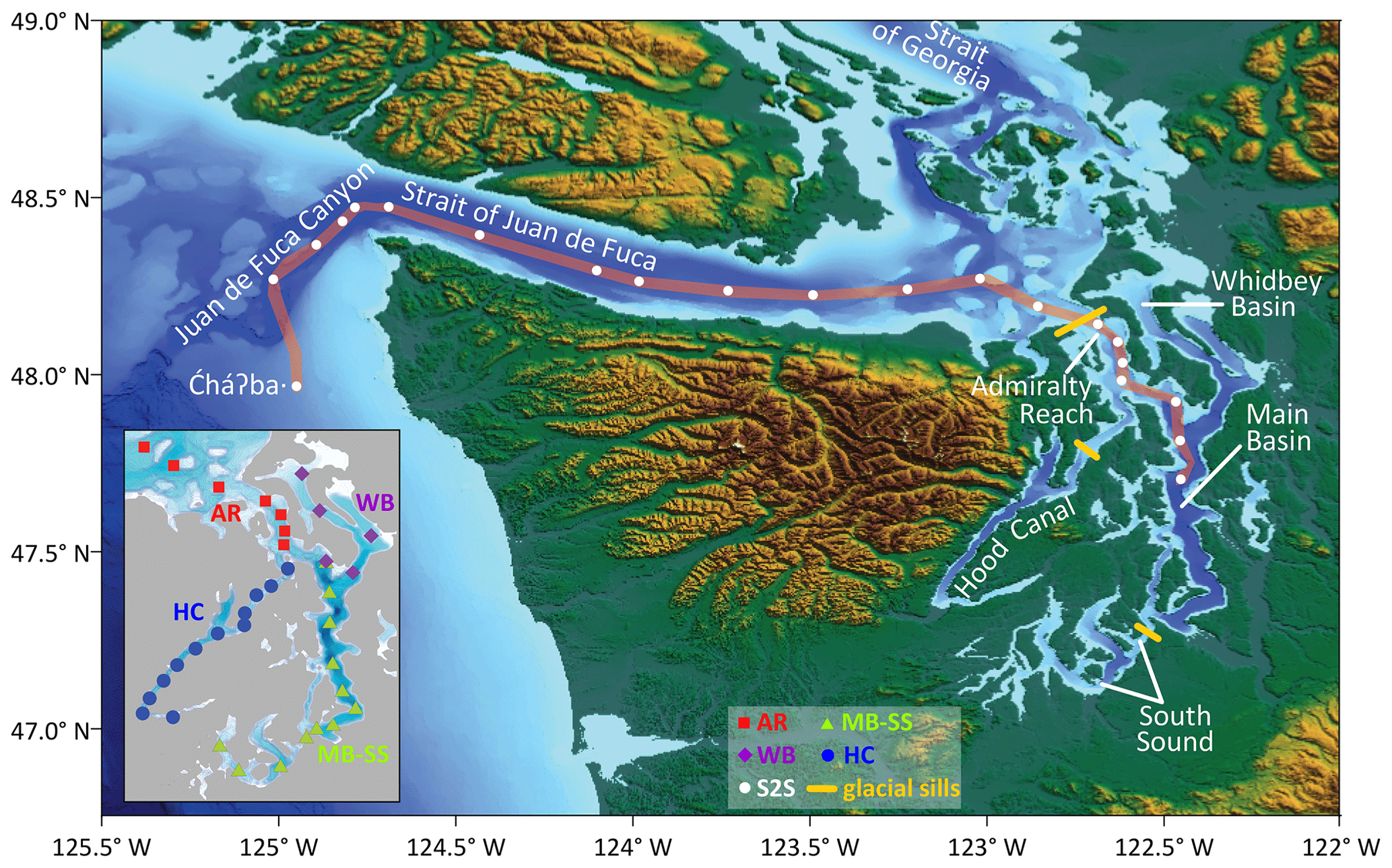
Figure 1 Map of the southern Salish Sea and its boundary waters with all study basins named (modified from Alin et al., 2024). The subset of sampling stations tracing a path between the “⋅” – meaning “whale tail” in the language of the Quileute Tribe – mooring on the Washington state (USA) continental shelf to the Main Basin of Puget Sound constitute the Sound-to-Sea (S2S) transects. The inset map shows the station groupings used for the analyses of Puget Sound cruises: Admiralty Reach (AR), Main Basin–South Sound (MB–SS), Whidbey Basin (WB), and Hood Canal (HC). Locations of glacial sills that restrict deep-water exchange in Puget Sound are shown. The Fraser River, mentioned in the text, enters the Strait of Georgia from the east, to the north of the map area. We extracted topographic and bathymetric data from the NOAA National Centers for Environmental Grid Extract Coastal Relief Model (3 s resolution, https://www.ncei.noaa.gov/maps/grid-extract/, last access: 13 November 2014). Data were gridded in Surfer using a minimum curve gridding technique.

The northern California Current ecosystem (CCE) provides the marine source water for deep waters within the southern Salish Sea and experiences episodic upwelling during spring–early fall (April–September) as a result of northwesterly equatorward winds causing offshore Ekman pumping (Huyer, 1983). Downwelling conditions occur during late fall–early spring (October–March) due to seasonal wind reversal to poleward-dominant winds along the coast. Upwelling conditions bring deep, nutrient-rich, CO₂-rich, O₂-depleted marine water masses into the Strait of Juan de Fuca from the Juan de Fuca Canyon (Fig. 1). This water transits at depth to the glacial sill complex at Admiralty Reach (AR), where it enters PS at depth during episodic marine intrusions. Strong freshwater outflow through SJdF, particularly during summer months when peak Fraser River discharge occurs, contributes to and enhances this estuarine circulation (Davis et al., 2014; Giddings et al., 2014). Strong tides and glacial sills within AR at the entrance to PS impart strong mixing – of outgoing warmer, fresher surface estuarine waters with colder, saltier marine waters entering PS from SJdF at depth; the strength of tides and resulting mixing influence the amount and characteristics of incoming marine water that refreshes deep water masses in all PS basins, and some of the outgoing estuarine water is refluxed back into PS (MacCready et al., 2021; MacCready and Geyer, 2024).

Glacial sills restrict estuarine circulation throughout the Salish Sea and among the PS basins as well, limiting marine intrusions and deep-water renewal to episodic occurrences and resulting in long residence and flushing times in some parts of this inland sea, including Hood Canal (Babson et al., 2006; Pawlowicz et al., 2007; MacCready et al., 2021). The Main Basin is the widest, deepest, and most deeply wind-mixed of the PS basins. Deep waters enter South Sound, the shallowest basin, from MB when they pass over another glacial sill at the Tacoma Narrows and undergo strong tidal mixing again while flowing into South Sound. Thus, the deeply mixed MB and SS share a deep-water transit path. In contrast, Whidbey Basin and Hood Canal have narrower basins than MB and major river inputs emanating from the terminus of each basin, resulting in strong stratification and gradients of physical and biogeochemical conditions between surface and bottom waters. HC is also bounded by a glacial sill and has a long history of study of deep-water oxygen concentrations, as hypoxia and fish kills have been observed there (Newton et al., 2011, 2012, and references therein). Observations and models for the Strait of Georgia suggest that mixing associated with glacial bathymetric features to the north of PS may afford some protection to deep northern Salish Sea basins, due to more rapid O₂ uptake than CO₂ outgassing (Johannessen et al., 2014; Ianson et al., 2016); this mechanism does not appear to protect Hood Canal from developing hypoxia. While not bounded by a glacial sill, circulation in WB is severely restricted at its northern outlet, and it receives strong river input in two locations. While WB has side inlets with hypoxia, the mainstem of the basin tends to see only moderately low oxygen values but no hypoxia.

Both regional weather and large-scale climate factors play important roles in driving physical, chemical, and biological processes in the Salish Sea and its boundary waters. From 2013 to 2016, an unprecedented marine heatwave (MHW) developed and persisted in the NE Pacific Ocean, followed by a very strong El Niño event in the equatorial Pacific Ocean during 2015–2016, both of which strongly influenced regional weather, oceanography, and ecosystems (e.g., Bond et al., 2015; Jacox et al., 2016; McClatchie et al., 2016; Morgan et al., 2019; N. Bond in Sobocinski, 2021). The NE Pacific heatwave's direct influence on Washington's coastal waters and the Salish Sea ecosystem began when anomalously warm waters from the North Pacific were advected onto the Pacific Northwest coast in mid-September 2014 (Peterson et al., 2017). However, associated strong, large-scale air temperature anomalies greatly influenced the surface PS system and preceded the arrival of the warmed ocean water masses (Swain et al., 2016), with anomalously warm, dry summer conditions starting in 2013 over the southern Salish Sea (Table 1, Fig. 2). As a result of these large-scale heat anomalies, PS and Washington coastal waters also experienced strong precipitation, river discharge, and solar energy flux anomalies during 2013–2018 (see Table 1 and references therein). Upwelling anomalies reflect basin-scale climate drivers and influence both the upwelling strength and the depth of marine source waters for deep waters of the southern Salish Sea (e.g., Jacox et al., 2015).

Table 1 Major environmental anomalies occurring during 2013–2018 and regional environmental drivers affecting the southern Salish Sea.

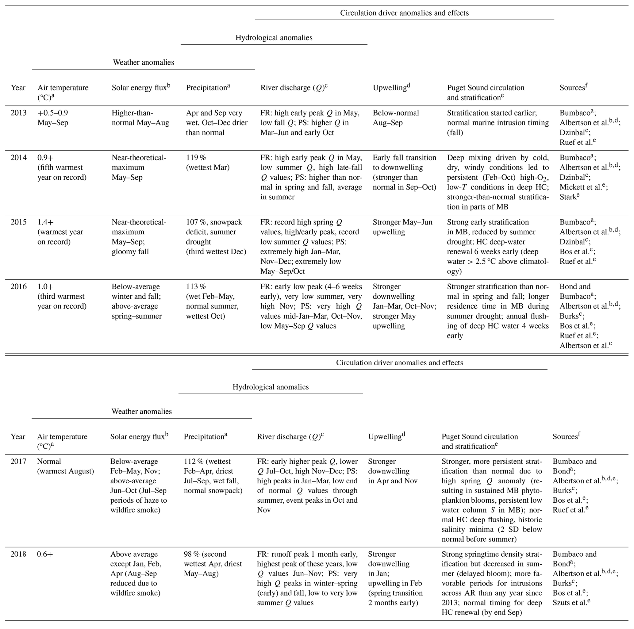
^a Annual and monthly average air temperature and precipitation anomalies are relative to the 1981–2010 normal. Record monthly, seasonal, or annual anomalies up to 2018 noted in parentheses. ^b Daily solar energy flux, an indicator of sunniness, measured in Seattle and compared to the highest theoretical solar energy for the latitude and time of year and fully overcast conditions. ^c River flows for the Fraser River (FR) – with a single summer discharge (Q, m³ s⁻¹) peak – are described relative to the median discharge from 1912 to the year reported. Puget Sound (PS) rivers – with an early summer snowmelt discharge peak and a late fall rainfall and winter storm discharge peak – are reported relative to the full length of their U.S. Geological Survey observational records, ranging from 47 to 104 years. ^d Upwelling anomalies are reported as monthly average upwelling index values (m³ s⁻¹ per 100 m of coastline) that fall outside the interquartile range (25 %–75 %) for 48° N, 125° W by NOAA's Pacific Fisheries Environmental Laboratory. Baseline period is 1967 to the year of each annual report. ^e Anomalies in Puget Sound stratification or deep-water renewal events were reported in temperature and salinity water quality narratives of annual marine conditions reports. ^f Sources for observations in previous columns are listed by authors of the relevant sections in the PSEMP Marine Waters Workgroup annual overview of marine conditions published in the following year (i.e., listed as citations in the relevant year's report: PSEMP Marine Waters Workgroup, 2014, 2015, 2016, 2017, 2018, 2019).

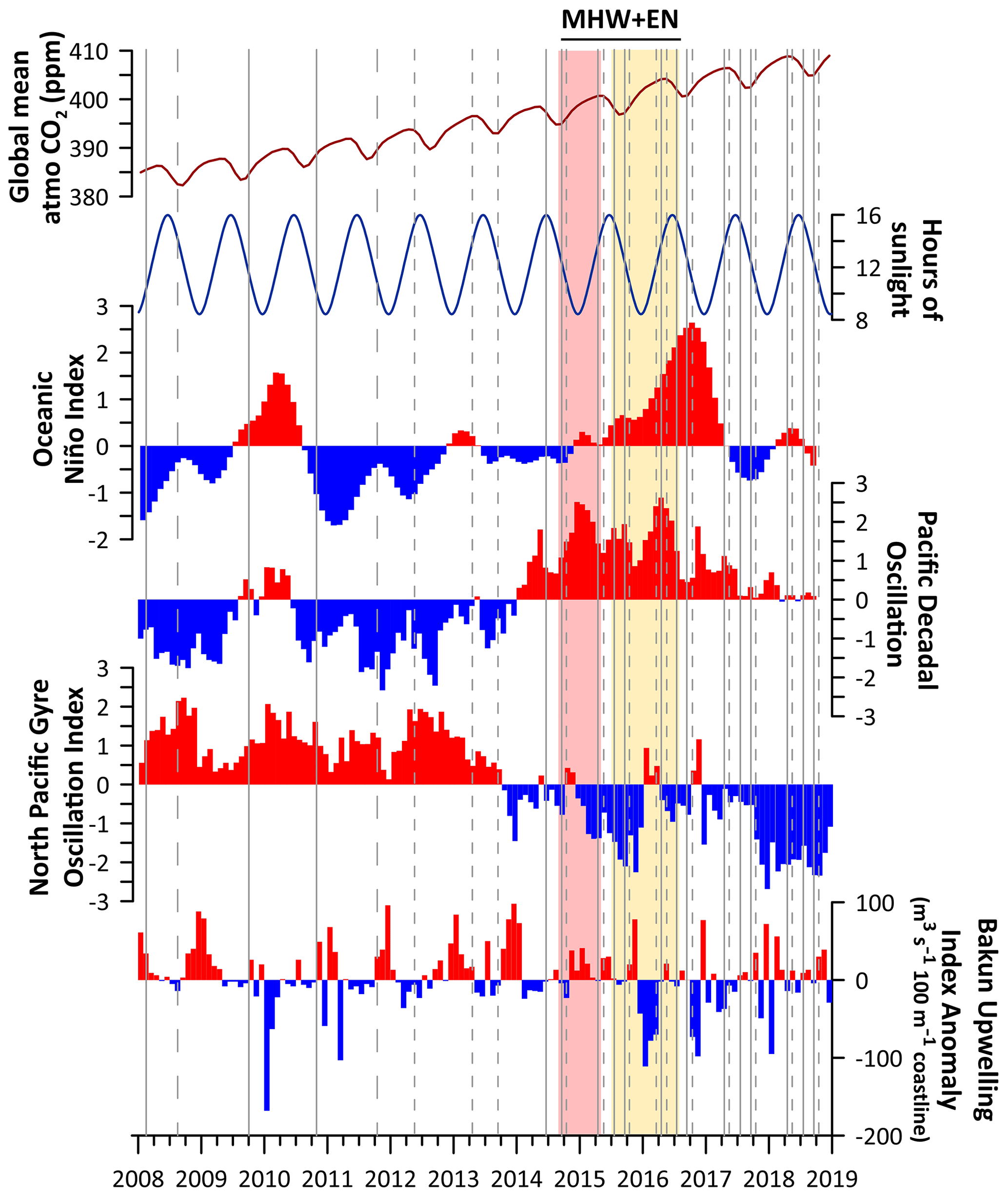
Figure 2 Monthly time series for 2008–2018 for the Oceanic Niño Index anomaly (NOAA Climate Prediction Center, 2019), Pacific Decadal Oscillation (Mantua, 2019), North Pacific Gyre Oscillation (Di Lorenzo, 2019), and Bakun Upwelling Index Anomaly for 48° N (NOAA Pacific Fisheries Environmental Laboratory, 2024). Positive anomalies for all climate indices are shown in red, whereas negative anomalies are shown in blue. Superimposed on this are the durations of the maximum intensity of the northeast Pacific marine heatwave (MHW), shaded in red during its peak manifestation in Washington marine waters (September 2014–April 2015) and in yellow for its later moderate-intensity window, which overlapped with the 2015–2016 El Niño event (EN, July 2015–July 2016). Duration and intensity ranges were inferred from Gentemann et al. (2017) and the OSU MODIS water temperature anomaly climatology tool (NANOOS, 2019). Overlap between the 2014–2016 NE Pacific heatwave and warm waters that may be the result of the El Niño can be seen by comparing the Oceanic Niño Index positive anomalies to the yellow shading, based on satellite sea surface temperature analysis associated with the marine heatwave (i.e., Gentemann et al., 2017). Seasonality is shown using hours of sunlight per day as a proxy, shown at the top (timeanddate, 2019). Finally, the timing of all Salish cruises is indicated by vertical lines, with Sound-to-Sea (S2S) cruises displayed using short-dashed lines, Puget Sound (PS) cruises displayed using solid lines, and the two cruises that encompassed both sets of stations displayed using long-dashed lines.

3 Methods: observations, calculations, and data visualization

3.1 Salish cruise time series

For this analysis of seasonal variability and oceanographic anomalies, we used the Salish cruise data product, comprising 35 consistently formatted and quality-controlled cruises data sets collected throughout the study region from 2008 to 2018 (Alin et al., 2022, 2024). The Salish cruise data product includes conductivity–temperature–depth (CTD) and discrete measurements collected on each cruise, including temperature, salinity, and oxygen measurements collected by sensors during CTD casts, and discrete water samples measured for oxygen, nutrients (phosphate, silicate, nitrate, nitrite, and ammonium), dissolved inorganic carbon (DIC), and total alkalinity (TA) content. Measurement uncertainties were ±0.01 °C, ±0.02, and ±2 % of saturation for temperature, salinity, and oxygen sensor observations, respectively. For laboratory analyses on discrete water samples, uncertainties were ±1 % for oxygen (precision), ±2 % for nutrients, and ±0.1 % (∼2 µmol kg⁻¹) for DIC and TA content. Data collection methods are explained in detail in the companion paper (Alin et al., 2024), with quality control following methods developed for identifying outliers in the Coastal Data Analysis Product in North America (CODAP-NA; Jiang et al., 2021).

The timing of both Puget Sound (PS) cruises and Sound-to-Sea (S2S) cruises has been particularly consistent and frequent since 2014, with 24 of the 35 cruises having taken place between July 2014 and October 2018. Thus, our analysis of seasonal patterns in ocean conditions spanning the upwelling season focuses on the period from 2014 to 2018 (Fig. 2) and will provide the oceanographic context for numerous biological oceanography studies that have also been conducted on the S2S and PS cruises. While each cruise represents a snapshot of conditions along a transect from the coast into the southern Salish Sea or across the basins within the southern Salish Sea, collectively this cruise time series illuminates typical spatial patterns throughout the southern Salish Sea, throughout the water column, and through the seasonal cycle.

3.2 Calculated parameters and uncertainty

DIC and TA measurements from the Salish cruise data product were used to calculate the full suite of inorganic carbon parameters, although our discussion of seasonal ocean acidification conditions and anomalies focuses on the calculated parameters fCO₂ and Ω_arag, as these are two of the inorganic carbon parameters most familiar to our science and resource management end users. Of the carbonate system parameters, fCO₂ is most directly relatable to atmospheric values and trends and, thus, has intuitive value, and Ω_arag is critical to many of the important calcifying species in the Salish Sea. For species and investigators for whom pH_T and Ω_calc are more relevant (e.g., Dungeness crab), complementary figures are provided in the Supplement.

We used the R seacarb package carb function to calculate all carbonate system parameters (Gattuso et al., 2023). Within seacarb, we used the TEOS-10 thermodynamic seawater equations option (IOC, SCOR, and IAPSO, 2010). We used Lueker et al. (2000) dissociation constants to facilitate comparison with results from West Coast Ocean Acidification (WCOA) cruise publications (e.g., Feely et al., 2008, 2016). We adopted the total scale for pH (pH_T), the Uppstrom (1974) formulation for deriving total boron concentration from salinity, the seacarb default option for K_f (Perez and Fraga, 1987, for temperatures above 9 °C; Dickson and Goyet, 1994, for those below), and the Dickson (1990) option for K_s (following results of Orr et al., 2015). Calculated values of fCO₂ shown in the figures here are the seacarb “in situ” CO₂ fugacity values, referenced to in situ temperature and pressure, rather than atmospheric pressure as the “standard” and “potential” options are computed (Gattuso et al., 2023), because in situ results are more germane to understanding the environmental conditions confronting populations of marine organisms in the wild. We use fCO₂ rather than pCO₂ as it provides the most accurate estimate for in situ gas-phase CO₂ (per recommendations in Jiang et al., 2022). Per Orr et al. (2018), total uncertainties on calculated values using high-quality DIC and TA measurements as input parameters are ±3.5 % for fCO₂ (±14 µatm at 400 µatm and ±70 µatm at 2000 µatm) and ±4.9 % for Ω_arag (±0.025 at Ω_arag=0.5, ±0.049 at Ω_arag=1, and ±0.075 at Ω_arag=1.5).

To facilitate the broad use of Salish cruise observations, including the calculated values discussed here, we created a new multi-stressor Salish cruise data product that includes all of the highest-quality (i.e., measurements with “acceptable” data quality flags) seacarb input data (temperature, salinity, DIC, and TA), O₂ and nutrient values in commonly used units, and the most frequently used carbonate system parameters (pH_T, fCO₂, pCO₂, Ω_arag, and Ω_calc) (Alin et al., 2023). We compare calculated CO₂ system values using Lueker et al. (2000), suitable for salinities of 19 to 43, versus Waters et al. (2014), suitable for salinities from 0 to 50, dissociation constants in the Supplement, because salinity across Salish Sea habitats spans ocean to freshwater values. Finally, we describe the magnitude of differences between fCO₂ and pCO₂ values in the Supplement. The CO₂ system variables calculated with both sets of dissociation constants as well as both fCO₂ and pCO₂ values are available in the Alin et al. (2023) data product.

3.3 Data visualization

Raincloud plots display both raw data and percentile distributions to provide transparent statistical data summaries (Allen et al., 2021). We use them to visually summarize the 2014–2018 statistical distributions of temperature, salinity, oxygen, fCO₂, and Ω_arag observations from May and October boundary water (S2S) cruises (Figs. 3a, 4a, 6a, 8a) and for April, July, and September PS cruises (Figs. 3b, 4b, 6b, 8b). Raincloud statistical summaries for potential density anomaly (sigma theta, σ_θ), Ω_calc, and pH_T are provided in Figs. S1–S3 in the Supplement for readers interested in this information. Raincloud plots were created using R code by Cédric Scherer (Scherer, 2024) but modified extensively for use with Salish cruise data. To characterize differences in median and extreme values for all parameters with depth, we used 20 dbar as the boundary between surface and subsurface depth categories throughout the region, although we acknowledge that mixing depths vary across the study region and seasons, such that the upper mixed layers occupy different depth ranges through space and time.

Transect plots of all calculated ocean acidification parameters (fCO₂, Ω_arag, Ω_calc, and pH_T) were prepared in Surfer and can be found in Figs. S4–S8. Comparable plots of temperature and salinity as well as oxygen, DIC, TA, and nutrient content are shown in Figs. 4–9 and S1–S4 of the companion article to this paper (Alin et al., 2024).

Bubble cloud plots are scatterplots in which additional statistics can be represented by the size and color of each data point. We used the R ggplot2 package ggpubr functions facet_grid and geom_point to create bubble plots summarizing seasonal changes in median values and ranges of T, S, O₂, fCO₂, and Ω_arag across the study region and by depth during 2014–2018 (Figs. 5, 7).

4 Results: seasonal variability in physical and biogeochemical parameters across depths and basins during 2014–2018

In this section, we describe seasonal oceanographic variation within and across basins for the latter half of the time series (2014–2018), including differences between surface and subsurface water masses, with ranges serving as our metric of variability. We note the timing and magnitude of apparent anomalies in median or variability for each parameter here and relate these physical and biogeochemical Salish cruise anomalies to the major 2013–2018 weather, hydrological, and circulation anomalies (Table 1) in Sect. 5, using existing climatologies to provide longer-term context. We refer to cruises occurring in April and May as “spring” cruises, July cruises as “summer”, and September–October cruises as “fall”. To denote specific cruises, we abbreviate the cruise by the first letter of the month (A, M, J, S, and O, respectively) and the two-digit year (e.g., October 2014 becomes O14). “Spring” cruises also reflect early-upwelling-season conditions, whereas July–September cruises represent late-upwelling-season conditions. The term “coastal” refers to stations outside the mouth of the Strait of Juan de Fuca (SJdF), sampling either deep Juan de Fuca Canyon (JdFC) stations or the ⋅ station in shallower water on the continental shelf (Fig. 1). All observations in this compiled cruise data product reflect open-basin conditions throughout PS and its boundary waters, which may be quite different from nearshore environments, such as the finger inlets of South Sound or seagrass meadows that may have markedly different circulation, freshwater influence, and retention times.

4.1 Physical oceanographic seasonality across basins

During 2014–2018, coastal surface temperature and salinity were largely dominated by seasonal upwelling/downwelling dynamics, as expected. Coastal surface temperatures spanned similar ranges in the early and late upwelling season, whereas deep coastal water had more of a seasonal contrast between the early and late upwelling season, with warmer water and wider T ranges in the fall (Fig. 3a, Table 2). Both surface and subsurface temperatures were warmer by nearly 3 °C during O14, when the MHW was strongest in coastal waters, with less-elevated temperatures in surface waters in M16 during the El Niño. Surface salinities were lower in spring than in fall, with somewhat fresher anomalies during M17 and O15. October cruises during 2016–2018 had higher surface salinities than O14 and O15 (Fig. 4a). However, deep fall salinities during 2014–2015 occupied larger ranges (Table 2). Potential density anomaly values (σ_θ) track salinity quite closely throughout this region (Moore et al., 2008) and are not discussed further here but are represented in Fig. S1. Depth distributions of physical parameters can be seen in more detail in Figs. 4–6 in Alin et al. (2024).

Seasonal patterns in Strait of Juan de Fuca surface waters were similar, with somewhat narrower surface temperature and salinity ranges than at coastal stations across the upwelling season (Figs. 3a, 4a). As seen at coastal stations, subsurface temperature and salinity in SJdF showed stronger variability, particularly in fall (Table 2). Temperature anomalies manifested as the widest ranges and highest medians during O14 across the water column, with some residual heat persisting in the form of wider ranges and higher medians across the water column in O15 and O16 relative to O17 and O18 when medians were lower. Subsurface salinity had higher medians than at the surface on all cruises and occupied wider ranges except during M18. Salinity had lower median values across the water column during O14, O15, and O16 than during O17 and O18.

AR showed a seasonal progression of warming between April and July–September cruises, with the median temperatures warming by 1–2 °C and variability increasing across depths (Fig. 3b). April temperatures were warmer across depths during 2015–2016 relative to 2017–2018, and a similar magnitude of warming was observed across depths between J14 and J15 (Table 2). The seasonal span of salinities at AR overlapped across depths, with greater variability at depth in all seasons (Fig. 4b). Median salinity increased across depths by a few salinity units from April to September each year as upwelled deep coastal waters arrived at AR by the end of the upwelling season. Median 2017 AR salinities decreased by ∼ 1 across the water column compared with other years, except at depth in S17.

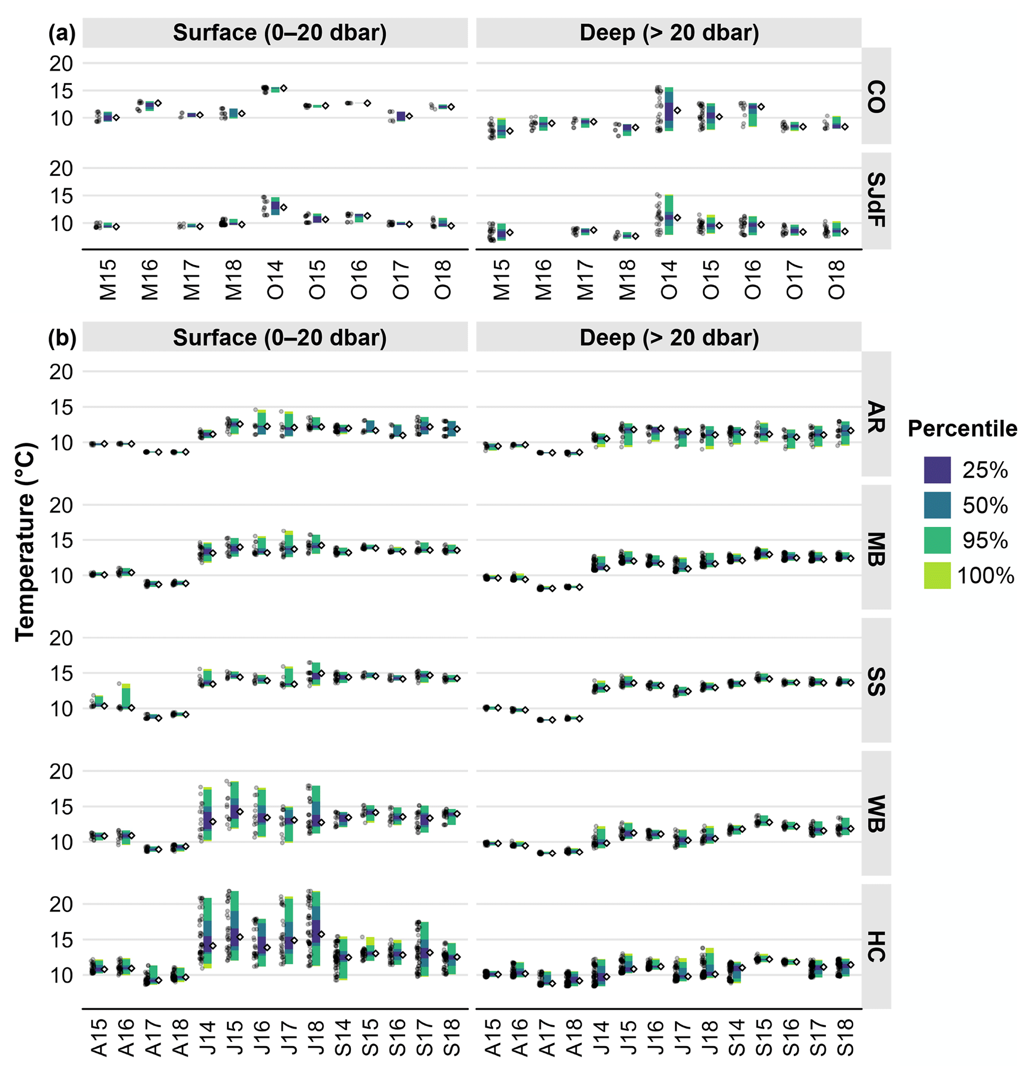
Figure 3 (a) Raincloud plots for CTD temperature in coastal (upper row) and Strait of Juan de Fuca (lower row) surveys in the early and late upwelling season beginning in the fall of 2014. Cruise timing is indicated with a one-letter month (M – May; O – October) and a two-digit year. Surface observations are in the left column, and subsurface observations are in the right column. Percentiles for observations are reflected by the colors of the vertical bars, similarly to a box plot, with the median displayed to the right of each bar as an unfilled black diamond and individual observations plotted to the left of each vertical bar as transparent gray circles. Note that all panels in this figure have the same scale bar but differ from those in the corresponding Puget Sound figure. (b) Raincloud plots for CTD temperature in Puget Sound regions – Admiralty (top row), Main Basin (second row), South Sound (third row), Whidbey Basin (fourth row), and Hood Canal (bottom row) – in April, July, and September beginning in July 2014. Cruise timing is indicated with a one-letter month (A – April; J – July; S – September) and a two-digit year. Surface observations are in the left column, and subsurface observations are in the right column. Percentiles for observations are reflected by the colors of the vertical bars, similarly to a box plot, with the median displayed to the right of each bar as an unfilled black diamond and individual observations plotted to the left of each vertical bars as transparent gray circles.

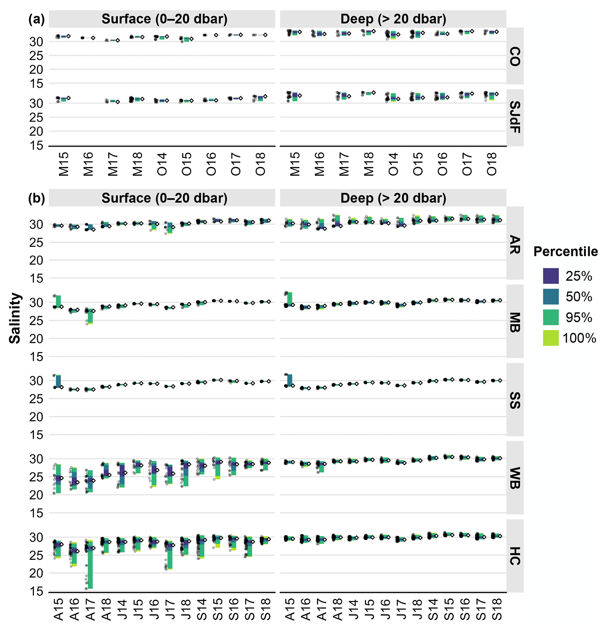
Figure 4 (a) Raincloud plots for CTD salinity in coastal and Strait of Juan de Fuca surveys in the early and late upwelling season beginning in the fall of 2014. Figure organization is the same as in Fig. 3a. (b) Raincloud plots for salinity in Puget Sound surveys in April, July, and September beginning in July 2014. Figure organization is the same as in Fig. 3b.

MB and SS are the least strongly stratified basins within PS; they show relatively weak gradients and narrow ranges in temperature and salinity from surface to deep waters, despite MB bottom depths reaching ∼ 225 dbar (Figs. 3b, 4b; Table 2). Due to deep mixing, MB and SS are often the warmest of all basins at depth. Temperatures increased by 2–4 °C between the April and July–September cruises in both surface and deep water, typically with 1–3 °C difference between surface and deep median temperatures (Fig. 3b). Salinity across depths showed progressive increases of ∼ 1–3 across the April–September cruises in a given year in both basins, with low variability across the water column (difference of ∼ 1 or less between surface and deep medians; Fig. 4b). April temperatures were ∼ 2 °C higher across depth in both basins during 2015–2016 than during 2017–2018. Median surface temperatures in J15 and J18 were elevated by ∼ 1–2 °C across MB and SS, and deep J15 and O15 median temperatures were <1 °C higher than in other years (Fig. 3b). High salinity outliers (by > 3 salinity units) were seen across depth in both basins during A15, and relatively low surface salinity medians were observed during A17 (outliers to ∼ 24) and J17 in MB and SS (Fig. 4b, Table 4).

WB and HC have the strongest stratification and gradients of physical and biogeochemical conditions between surface and bottom waters in PS (Figs. S5–S8 in this paper; Figs. 5–9 and S1–S4 in Alin et al., 2024). At the entrance to HC, deep-water replacement is constrained by an additional glacial sill and influenced by further mixing of surface with deep water. Subsurface waters in both basins warmed continuously from the April through September cruises each year, as they did in MB (Table 2). Deep-water salinity also increased steadily between April and September across WB and HC, with the only obvious anomaly among years being lower salinity in deep WB waters during A17 (lower by ∼ 2). Surface waters in WB and HC were the most variable of all regions for temperature and salinity. The widest ranges of surface temperature occurred in WB and HC during Julys, although median surface temperatures were similar between Julys and Septembers of each year in WB and warmest during July cruises in HC, with cooling by Septembers. Surface salinity tended to be highest and ranges narrower in Septembers, with considerable interannual variability during 2014–2018. Surface temperature anomalies were seen in higher medians in J15 and J18 in HC and J15 in WB as well as at depth in both basins in S15, while A15 and A16 had medians ∼ 2 °C warmer across depth in both basins compared with A17 and A18 (Fig. 3b). A16 and A17 had lower median salinities in both WB and HC than A15 or A18 (Fig. 4b). All 2017 cruises had anomalously wide ranges and low outliers for salinity in HC.

To summarize across years, regions, and parameters, Fig. 5 shows that PS temperature ranges were mostly shifted up relative to the boundary waters across depths, with higher medians and wider ranges everywhere in summer and fall than spring (see also Table 2). As expected, median salinity was consistently fresher in PS than boundary waters, with substantially wider overall ranges (Fig. 5). Vertical temperature and salinity gradients (surface median–deep median) were weakest at the AR and SS stations. Temperature gradients were weakest in spring and strongest in summer, while salinity gradients were strongest in spring and weakest in fall. HC summertime temperature gradients were the strongest (4.5 °C), with WB usually having the strongest salinity variability and surface–deep gradients (4.5 salinity units). While surface variability in T and S tended to be higher in PS surface waters, boundary waters typically showed greater subsurface variability.

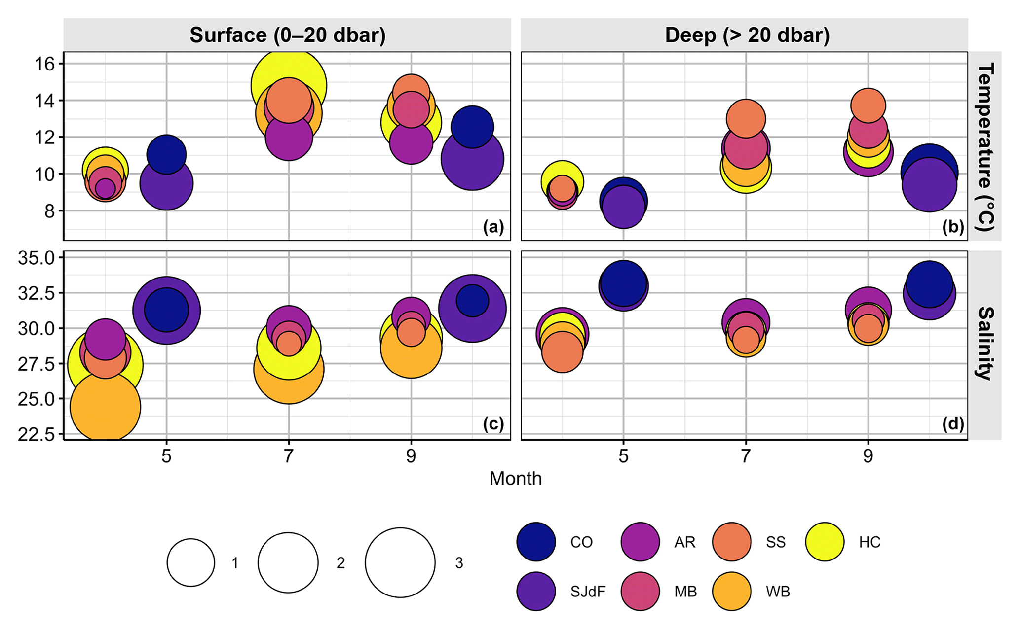
Figure 5 Bubble plots of summary statistics for the physical oceanographic parameters – temperature (a, b) and salinity (c, d) – in surface (a, c) and deep (b, d) water. Bubbles are plotted by the magnitude of mean monthly medians for each parameter taken across Washington Ocean Acidification Center (WOAC, April, July, and September) and Sound-to-Sea (S2S, May and October) cruises during 2014–2018. Bubbles are filled with colors representing the basin that the observations were derived from (CO – Coast; SJdF – Strait of Juan de Fuca; AR – Admiralty Reach; MB – Main Basin; SS – South Sound; WB – Whidbey Basin; HC – Hood Canal). The area of the bubble represents the average range width for that parameter across 2014–2018 WOAC or S2S cruises. The bubble sizes in the legend represent the upper ends of four bins of average range widths (i.e., maximum–minimum) for each parameter: temperature range bins are 0.0–2.5, 2.5–5.0, 5.0–7.5, and 7.5–10.0 °C; salinity range bins are 0.0–2, 2–4, 4–6, and 6–8. Bubbles are ordered such that those with the largest ranges are at the back. Thus, if a basin is not visible, its range overlaps completely with another basin's range.

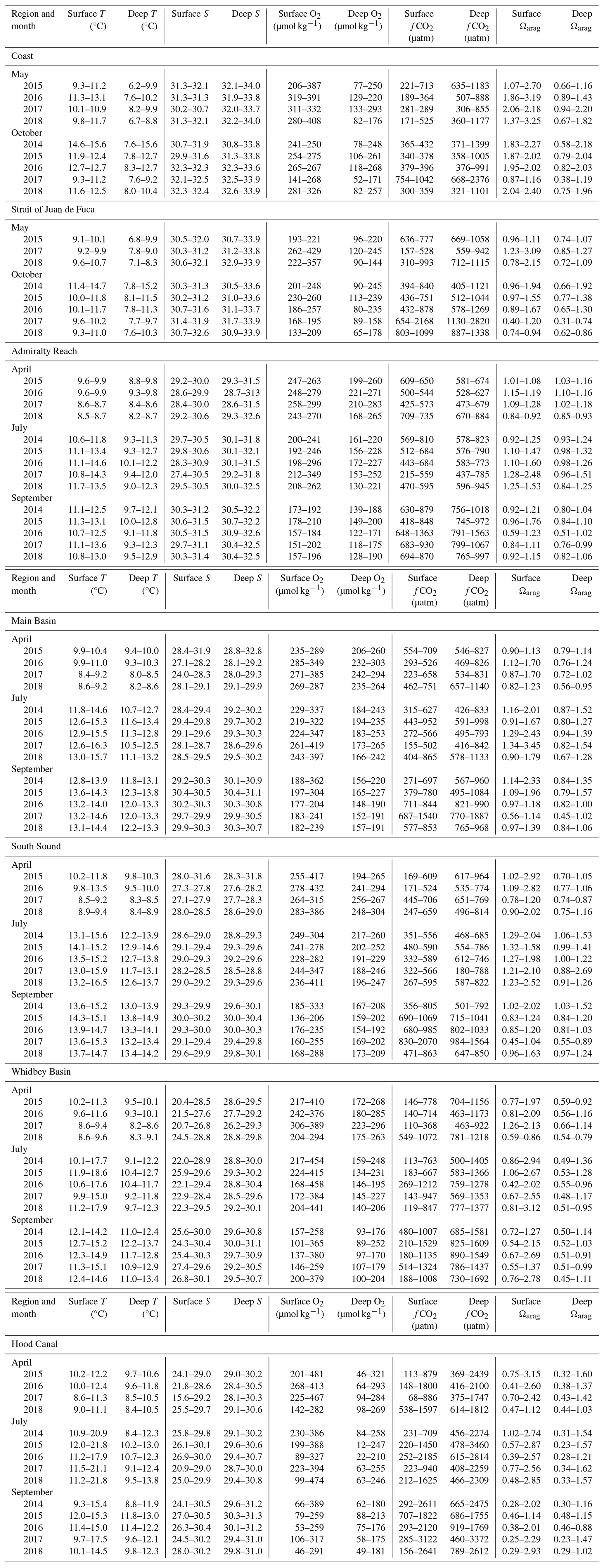
Table 2 Ranges of surface (≤20 dbar) and deep (>20 dbar) temperature (T, ITS-90 – International Temperature Scale of 1990), salinity (S, PSS-78 – Practical Salinity Scale), oxygen (O₂), and calculated values of CO₂ fugacity (fCO₂) and aragonite saturation state (Ω_arag) for all regions.

4.2 Biogeochemical seasonality across basins

4.2.1 Dissolved oxygen

Wide ranges of oxygen content were seen at coastal and SJdF stations, at surface and subsurface depths. Deep-water oxygen observations frequently had higher variability than surface waters, with strong interannual variability in O₂ medians, which were all above the hypoxia threshold (i.e., 62 µmol kg⁻¹ = 2.0 mg L⁻¹ = 1.5 mL L⁻¹), and ranges that occasionally dipped into hypoxic conditions (Fig. 6a, Table 4). No clear seasonal difference in deep O₂ content emerged between early and late in the upwelling season, but deep-water O₂ medians were lower during O17, M18, and O18 in boundary waters. Boundary water surface O₂ medians were consistently higher than subsurface values during any single cruise, although ranges sometimes overlapped across depths. Surface ranges were wider at SJdF stations, but subsurface ranges were widest at the coastal stations.

Oxygen content in deep AR waters decreased in median, minimum, and maximum values from April to September each year (Fig. 6b). Surface O₂ also showed decreasing median values from April to September, but surface ranges were narrower than at depth in spring and fall, such that surface O₂ observations ranges in April and September did not overlap. Wider O₂ ranges and higher outliers were observed during J16 and J17 at the surface, and wider ranges with low outliers were seen at depth during A17, J17, A18, and J18.

Open waters of MB and SS were consistently well oxygenated to the bottom (Fig. 6b, Table 4). MB bottom water oxygen was >220 µmol kg⁻¹ in spring and declined to median values of ∼ 160–180 µmol kg⁻¹ during September surveys (Fig. 6b; cf. Fig. 9 in Alin et al., 2024). Deep waters in SS only fell below 180 µmol kg⁻¹ twice, with minimum values of <160 µmol kg⁻¹ during S16 and S17. The O₂ content in MB and SS surface waters was always >200 µmol kg⁻¹ during April and July cruises, and occasionally medians were >300 µmol kg⁻¹ (e.g., A16 in both basins and A17 and J17 in MB). Across seasons, variability was higher in surface than deep waters, with generally decreasing median values throughout the water column from April to September.

Surface waters in WB and HC had wide ranges of O₂ through spring–fall cruises, typically with lower median O₂ content in Septembers compared with Aprils or Julys, particularly in HC (Fig. 6b). Subsurface O₂ variability was lower in WB, but O₂ variability remained high in HC deep water (Table 2). A progressive April–September decline in subsurface O₂ medians was observed in WB, although variability declined more consistently than medians in HC across seasons. Lower surface O₂ medians were observed during J16, A18, and J18 in WB and HC, with higher medians in A15, S15, A16, and S18 in WB. Deep WB waters had higher median values in A17 and high outliers in S15. In deep HC waters, median O₂ values in A17 appear higher than normal, while J15 and J16 O₂ medians and minima were ∼ 25–50 µmol kg⁻¹ lower than other Julys. The only measurements of hypoxic conditions in PS were taken in HC, at depth during S14, A15, J15, J16, S17, and S18 cruises, and in surface waters during S16 and S18.

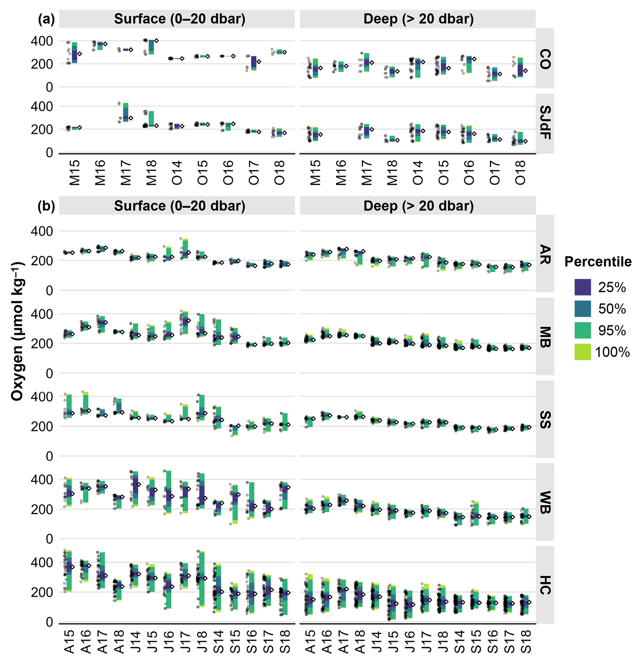
Figure 6 (a) Raincloud plots for adjusted CTD oxygen in coastal and Strait of Juan de Fuca surveys in the early and late upwelling season beginning in the fall of 2014. Figure organization is the same as in Fig. 3a. (b) Raincloud plots for adjusted CTD oxygen in Puget Sound surveys in April, July, and September beginning in July 2014. Figure organization is the same as in Fig. 3b.

Looking across basins, the surface oxygen content occupied similar overall range widths in spring and fall, while medians declined seasonally by 35–125 µmol kg⁻¹ everywhere (Fig. 7, Table 2). Surface O₂ variability was highest across seasons in HC, WB, and SJdF and lowest in AR. Surface variability was highest in summer in PS basins except SS, where it was lowest. WB surface O₂ medians and range width peaked and were highest among PS basins in summer, approaching spring coastal surface O₂ median values. Everywhere else, surface O₂ medians decreased from spring to fall. At depth, the O₂ content decreased monotonically by 52–94 µmol kg⁻¹ across all PS basins from April to September, with the largest decrease at AR and the smallest decrease across seasons in HC. In contrast, median O₂ in deep boundary waters remained roughly the same from spring to fall, with variability often exceeding surface variation. Ranges in deep O₂ content were widest in HC during spring–summer, followed by coastal and SJdF stations. While we observed hypoxic conditions in surface waters and near-anoxia at depth in HC, O₂ concentrations below the hypoxia threshold were not observed elsewhere in PS during these cruises. O₂ concentrations were consistently second lowest at the river end of the WB basin, with the lowest O₂ conditions occurring consistently in September, even during heatwave years when deep HC O₂ was lowest during the Julys.

4.2.2 Carbon dioxide fugacity (fCO₂)

Subsurface fCO₂ values typically had lower highs, lows, and medians at coastal stations than at SJdF stations (Figs. 7a, S4; Table 2). Coastal surface median values were, thus, often undersaturated with respect to atmospheric fCO₂, whereas SJdF medians were often above atmospheric values. As for O₂, no clear seasonal fCO₂ difference was evident, either at the surface or at depth. Coastal stations had higher surface median fCO₂ in M15, but the most notable variation was the anomalously wide fCO₂ ranges observed during O17, with deep-water medians > 1000 µatm at coastal stations (high = 2376 µatm) and ∼ 1900 µatm at SJdF stations (high = 2820 µatm). O17 SJdF surface fCO₂ values were unprecedented, with a median of 1575 µatm and highs of up to 2168 µatm. Coastal surface fCO₂ anomalies were also notable during O17, with the only observations of fCO₂ > 1000 µatm occurring then. SJdF M18 subsurface and O18 median fCO₂ observations across depth were also somewhat elevated compared with other cruises, suggesting possible carryover of the anomalously acidified water masses from the previous fall.

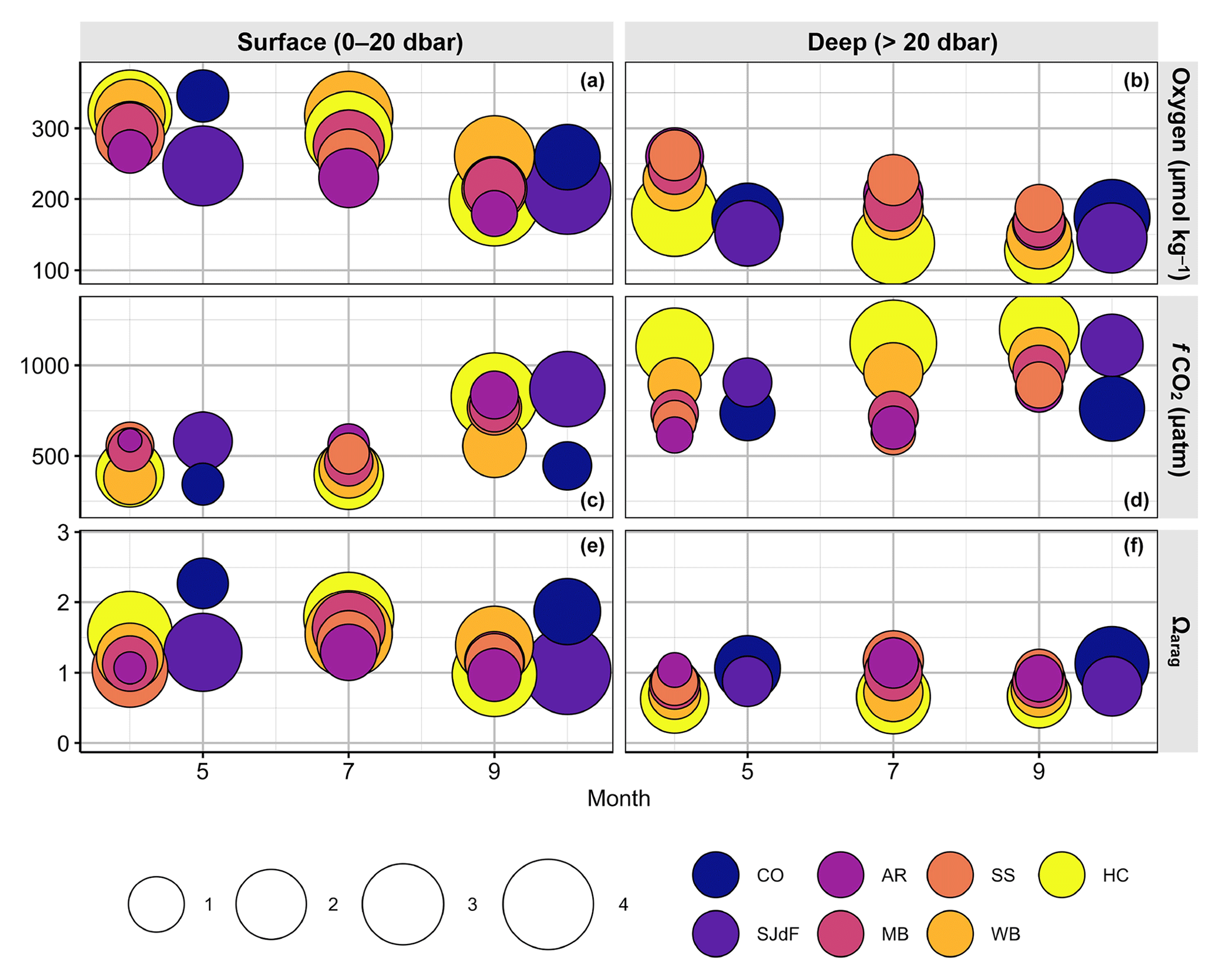
Figure 7 Bubble plots of summary statistics for the biogeochemical oceanographic parameters – oxygen content (a, b), fugacity of CO₂ (fCO₂, c, d), and aragonite saturation state (Ω_arag, e, f). Figure organization is the same as Fig. 5, with surface values in panels (a), (c), and (e), and deep values in panels (b), (d), and (f). Bubble size bins for biogeochemical parameters are 0.0–62.5, 62.5–125, 125.0–187.5, and 187.5–250.0 µmol kg⁻¹ for oxygen content; 0–600, 600–1200, 1200–1800, and 1800–2400 µatm for fCO₂; and 0.1–0.6, 0.6–1.1, 1.1–1.6, and 1.6–2.1 for Ω_arag.

AR fCO₂ medians and ranges increased between April and September, with most cruises having narrow ranges and little depth structure (Figs. 8b, S5; Table 2). The relatively wide overall AR fCO₂ ranges reflect low surface outliers in J17 and high outliers across depths in S16. The latter co-occurred with the lowest O₂ median in AR surface waters in this cruise time series (cf. Fig. 6b).

In MB and SS, fCO₂ variability across depths was lower during April–July than during September (Figs. 8b, S5; Table 2). The majority of the MB and SS observations >1000 µatm were associated with extremely high fCO₂ anomalies in S17. Extreme fCO₂ conditions in S17 were preceded by anomalously low fCO₂ in MB surface waters in J17 and, to a lesser extent, in A17, which we interpret as reflecting a protracted season of biological drawdown due to the co-occurrence of high O₂, low fCO₂, and sustained high chlorophyll (PSEMP Marine Waters Workgroup, 2018).

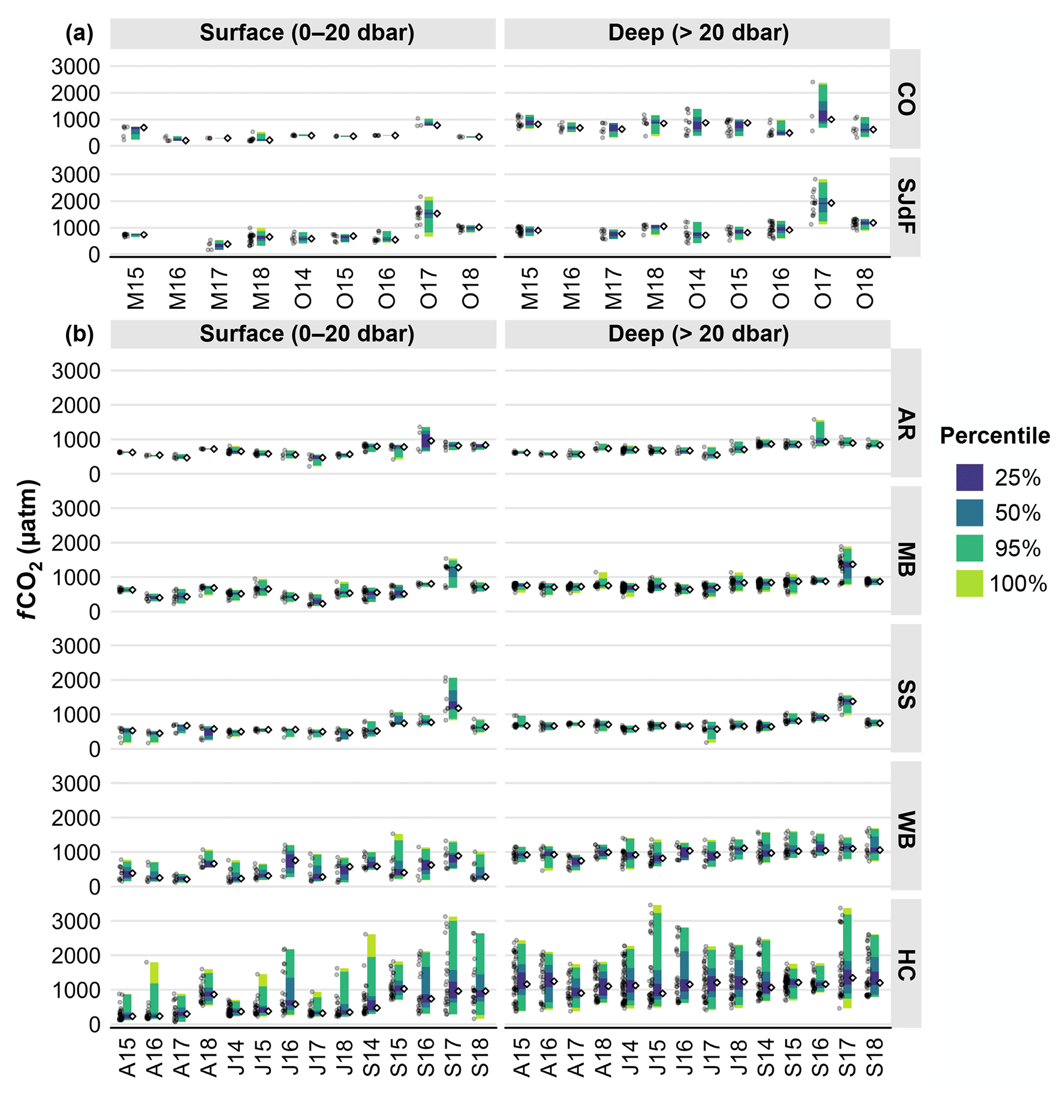
Figure 8 (a) Raincloud plots for the fugacity of CO₂ (fCO₂) in coastal and Strait of Juan de Fuca surveys in the early and late upwelling season beginning in the fall of 2014. Figure organization is the same as in Fig. 3a. (b) Raincloud plots for fCO₂ in Puget Sound surveys in April, July, and September beginning in July 2014. Figure organization is the same as in Fig. 3b.

Variability in fCO₂ was highest across regions in HC and second highest in WB, with similar range widths in surface and subsurface waters in both basins (Figs. 8b, S5; Table 2). Surface fCO₂ medians tended to be lower Aprils and Julys in both basins. HC had higher high fCO₂ values across depths and months than WB. Cruise medians were within ±230 µatm between WB and HC surface waters in Aprils and Julys, but HC surface water medians were more supersaturated with fCO₂ in all Septembers except S14. HC surface waters had particularly high fCO₂ outliers during S14, S17, and S18, with the highest deep-water HC values seen during J15 and S17. WB surface fCO₂ had the highest outliers during S15 and an anomalously high median during A18, which could reflect persistence of acidified conditions from fall 2017.

The majority of the water column was supersaturated with respect to atmospheric fCO₂ values (i.e., >400 µatm) in most places and times for the duration of this time series (Tables 4, 5), reflecting the importance of respiration processes in Salish Sea CO₂ chemistry, although moored time series show that surface undersaturation prevails in spring–summer (Alin et al. in PSEMP Marine Waters Workgroup, 2021; Fassbender et al., 2018). Average surface fCO₂ medians and ranges were lower and narrower, respectively, during spring and summer months than in fall across regions. As for temperature, salinity, and oxygen, HC, WB, and SJdF had the largest surface variability (Fig. 7). Median surface fCO₂ values were lowest across coastal, WB, and HC stations in spring and in HC and WB among PS basins in summer. The highest spring surface median values were in SJdF and AR, reflecting vigorous mixing bringing deep CO₂-rich waters to the surface. In fall, HC had comparably high surface median fCO₂ values to SJdF and AR, with the highest variability in HC and SJdF. In deep water, median fCO₂ values were higher than at the surface across seasons by ∼ 30–400 µatm at AR, MB, SS, and boundary water stations and by ∼ 350–725 µatm in WB and HC. Surface and deep fCO₂ levels overlapped most at AR in all seasons and in HC during fall, when local upwelling brings deep water enriched in fCO₂ to near-surface depths as it is flushed out of the basin via estuarine circulation (Figs. 8, S5). Median deep fCO₂ values were highest in HC across seasons, although SJdF and WB approached HC levels at depth during fall cruises. Coastal deep median fCO₂ values were comparable to MB and SS and higher than AR values in spring but lowest across regions in fall.

4.2.3 Aragonite saturation state (Ω_arag)

Both surface and subsurface boundary water Ω_arag spanned undersaturated to quite supersaturated (>1) values, with strong surface variability and lower highs and lows in SJdF (Fig. 9a, Table 2). Spring surface Ω_arag ranges were wider in both regions than fall ranges, with more variable median values, particularly at the coast. The highest deep medians occurred in O14 in SJdF and O16 at coastal stations, and the lowest medians were seen in O17 in both regions. Notably high surface median Ω_arag values were observed in M16 and M18 at coastal stations and M17 at SJdF stations, with notable surface low medians during O17 at both coastal and SJdF stations, as well as during M15 at coastal stations.

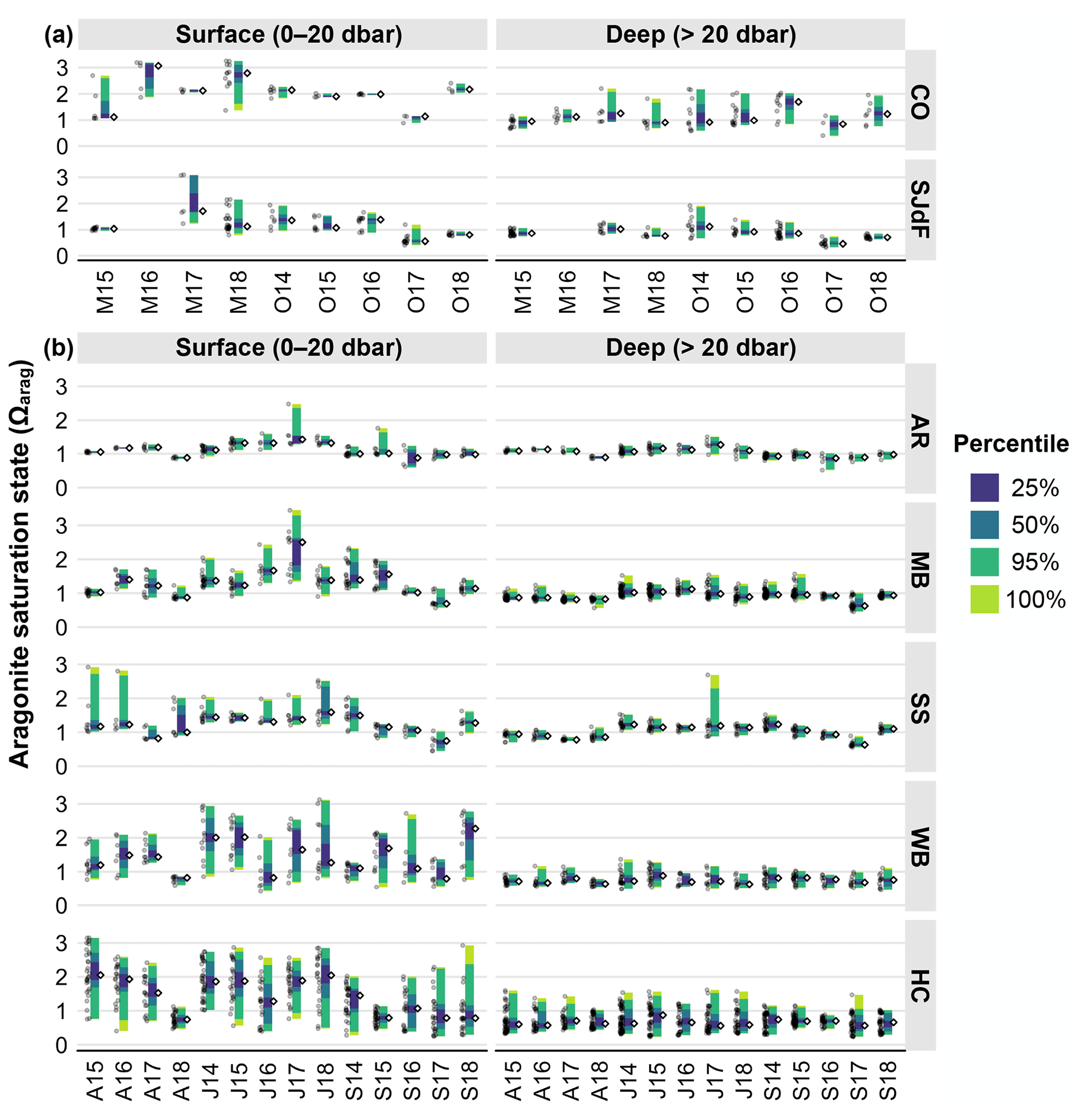
Figure 9 (a) Raincloud plots for aragonite saturation state (Ω_arag) in coastal and Strait of Juan de Fuca surveys in the early and late upwelling season beginning in the fall of 2014. Figure organization is the same as in Fig. 3a. (b) Raincloud plots for Ω_arag in Puget Sound surveys in April, July, and September beginning in July 2014. Figure organization is the same as in Fig. 3b.

In contrast to O₂ and fCO₂, surface Ω_arag medians at AR tended to be highest in Julys, followed by Aprils, with Septembers having the lowest values. The same pattern was evident but weaker at depth at AR. Ranges for Ω_arag were typically widest in July (Table 4). Anomalously wide ranges in Ω_arag were seen in surface waters with high anomalies in S15 and J17 and with a lower median and lows in S16.

Whereas fCO₂ variability was similar across depths in MB and SS, Ω_arag generally had substantially higher variability in surface waters than at depth (Fig. 9b, Table 2). Both surface and subsurface MB and SS waters had highest Ω_arag medians in Julys, with lower medians and significant interannual variability across Aprils and Septembers. Median deep SS Ω_arag observations were above saturation during Julys and some Septembers, whereas MB subsurface medians were typically below the saturation threshold (Ω_arag=1), reflecting the greater volume of deep water in MB. Exceptions occurred during J14, J15, and J16, when MB deep waters had medians >1, and J17 in SS, which had high deep-water outliers. Median surface Ω_arag values were supersaturated for all cruises except A18 in MB, A17 in SS, and S17 in both basins. Notably high Ω_arag outliers in surface waters were observed during A15, A16, and J18 in SS and J17 in MB, which also had the highest median observed across all basins and seasons in PS. Notably low Ω_arag medians occurred in S17 in both basins and across depths.

In WB and HC, Ω_arag ranges were much wider in surface than subsurface waters, with wider ranges at both depths in HC than WB (Table 4). Ω_arag ranges tended to be widest in WB surface waters in July, with no clear seasonal pattern in surface medians (Fig. 9b). Notable WB surface Ω_arag medians were >2 in J14, J15, and S18 and <1 in A18, J16, and S17. Surface HC Ω_arag medians were notably low in A18 and J16 and high in S14 (Figs. 9b, S6). Deep-water Ω_arag medians were more stable across months and consistently undersaturated.

In summary, median aragonite saturation states were substantially higher in surface coastal waters in spring and fall than throughout the SJdF and PS basins (Fig. 7). HC had the highest surface variability across seasons, with the highest PS medians in spring and summer and the lowest in fall. AR had the least inter- and intra-seasonal variability in all regions in both surface and deep water. Deep HC medians were lowest across months, with consistently high variability reflecting considerable along-basin gradients at depth (Fig. S6). Deep WB Ω_arag medians fell between those for PS and HC, but the range widths were more similar to PS basins than HC. Notably low Ω_arag anomalies occurred in fall 2017, with indications that acidified conditions were held over until A18, as observed in multiple basins.

4.3 The role of distinct seasonality across parameters and basins in driving the severity of acidification and hypoxia

Average ocean conditions from the coast through PS are summarized in bubble plots of each parameter for each month, region, and depth across all 2014–2018 cruises (Figs. 5, 7). Seasonal variation in median values and ranges across basins was not consistent across parameters. For instance, surface salinity seasonality was different from temperature seasonality across PS basins. Surface water temperatures peaked in some PS basins in summer, following solar radiation (Fig. 2), while deep-water temperatures continued to rise until fall, except at AR (Fig. 3b). In contrast, PS salinities progressively increased and ranges contracted from spring to fall, tracking seasonal precipitation and river discharge patterns (Fig. 4b, references in Table 1, and Banas et al., 2015). The continued increase in deep temperature and salinity until fall reflects a combination of surface conditions mixing to depth and the influence of upwelling bringing colder, saltier, lower-oxygen water masses into the Salish Sea and displacing the fresher, warmer, more-oxygenated water masses that are present in MB and SS in winter. Moored time series provide a longer-term, more temporally resolved context for the seasonal variability across parameters and PS basins observed in the Salish cruise time series and confirm that water mass properties do not vary consistently across PS basins. Specifically, HC deep-water seasonal peaks and troughs for temperature lag those from other basins by a few months (https://nwem.apl.washington.edu/prod_PS_ClimateTrends.shtml, last access: 20 March 2024). Salinities reach their peaks and nadirs 1–2 months after temperature in both surface and deep waters across all PS moorings.

The O₂ medians in most basins and across depths declined steadily from spring to fall, whereas Ω_arag medians across depths usually peaked in summer and fCO₂ levels typically increased most substantially by fall (Fig. 7). Variability in O₂ and Ω_arag was markedly lower in subsurface than surface waters, although deep-water HC ranges were still wide (Figs. 6, 9; Table 2). However, subsurface fCO₂ ranges were typically as wide as surface ranges or, in the case of HC, often wider (Fig. 8, Table 2), which likely reflects the amplification of fCO₂ variability that occurs when buffering capacity declines (Pacella et al., 2018; Kwiatkowski and Orr, 2018).

Oxygen and inorganic CO₂ dynamics often mirror each other within a local water mass because they are linked by the stoichiometry of biological production and respiration processes, but these can be decoupled across depth (e.g., Cai et al., 2011; Feely et al., 2010). Surface fCO₂ and O₂ levels dominantly reflect phytoplankton bloom activity, which peaks from spring to summer throughout the study region (e.g., PSEMP Marine Waters Workgroup, 2019, and earlier years). Organic matter from phytoplankton blooms subsequently drives the regional spring to fall O₂ decrease and fCO₂ increase via respiration in both surface and subsurface waters. While CO₂ drawdown also affects saturation states, Ω_arag peaked in summer in many basins, reflecting a stronger temperature influence on carbonate ion concentrations than fCO₂ in surface waters (Fig. 1 in Cai et al., 2020). In deep water masses, biogeochemical parameters tended to follow more monotonic seasonal trajectories, with T, S, and fCO₂ increasing and O₂ decreasing across spring–fall as a result of longer residence times and respiration contributing to higher fCO₂ (e.g., Feely et al., 2010, 2024). Thus, seasonal decoupling across metrics of ocean acidification and oxygenation reflects the relative importance of physical versus biological control on each parameter, which have strong gradients across the estuarine to coastal to open-ocean continuum (Kwiatkowski and Orr, 2018; Lowe et al., 2019; Cai et al., 2020).

Interpreting Salish cruise seasonal patterns in the context of the moored climatologies across PS shows that deep climatological temperature and salinity minima tend to co-occur with maximum annual deep O₂ values and vice versa from AR to SS, whereas annual low and high values of T, S, and O₂ occur synchronously in HC. The lag in temperature and salinity seasonality in deep HC waters is consistent with the longer residence and transit times along the deep axis of HC compared with other basins (Babson et al., 2006; MacCready et al., 2021). While deep-water renewal in the MB, SS, and WB basins follows mixing of incoming upwelled water with outgoing surface water at AR, deep-water renewal in HC requires incoming marine waters to pass over a second glacial sill before transport along the long deep axis of HC, contributing to lags in temperature and salinity seasonality in deep HC waters. Consequently, midsummer to fall bottom water in HC was often colder and fresher than in MB and SS, while bottom water toward the southern end of the HC basin was frequently warmer and saltier in winter–spring (Figs. 5 and 6 in Alin et al., 2024). Peak surface O₂ values occur earliest in HC, followed by SS and AR, with MB peaking latest, spanning spring to summer. Climatological low surface O₂ values span fall to winter, occurring earliest at AR, followed by MB, SS, and finally HC. Collectively, these observations suggest that the earlier surface O₂ peak (fCO₂ nadir) in HC surface waters, which (along with higher chlorophyll values) implies an earlier seasonal onset and peak of primary production (PSEMP Marine Waters Workgroup, 2018), translates to earlier O₂ depletion in deep waters driven by remineralization of sinking phytoplankton. The earlier peaks in production and respiration in HC thus effectively offset the deep-water lag in O₂ minimum (and fCO₂ maximum) timing relative to T and S seasonality seen in other basins. This is important because the interaction and timing of seasonal peaks in physical and biogeochemical processes drive the formation of hypoxic, corrosive conditions in HC deep waters. Thus, future changes in deep-water renewal timing – as observed during the MHW – and the phenology of surface biological processes may influence deep-water conditions differently across the distinct basins of this complex ecosystem and could result in new acidification or hypoxia hotspots emerging.

5 Discussion: how did major environmental anomalies of 2013–2018 affect physical and biogeochemical conditions?

The 2014–2016 part of the Salish cruise time series coincided with the protracted, intense heat anomaly initiated by the 2013–2015 NE Pacific marine heatwave (MHW) and extended by the 2015–2016 El Niño event (Bond et al., 2015; Jacox et al., 2016; Gentemann et al., 2017; Peterson et al., 2017). The combination of the Pacific Ocean heat anomalies and a protracted atmospheric heat anomaly affecting the western US during 2014–2015 (Swain et al., 2016) altered atmospheric and seawater temperatures in the Salish Sea (Table 1 and references therein). Record precipitation occurred during at least 1 month per year throughout 2014–2018, with river discharge timings showing strong anomalies tending toward earlier, higher peak runoff and lower summer flows than in the historical baseline (Table 1 and references therein). In the following, we connect how the timing of these environmental anomalies contributed to the oceanographic anomalies observed in Washington's marine waters, focusing on understanding the genesis of summer and fall deep-water anomalies, because the strongest hypoxic and acidified conditions typically occur then. We focus on the oceanographic responses of boundary waters, weakly stratified MB, and strongly stratified HC to examine whether the 2013–2018 environmental anomalies caused changes in the timing or decoupling of physical or biogeochemical processes (such as those described in Sect. 4.3) and, in so doing, worsened or ameliorated ocean acidification and hypoxia at new locations or times.

5.1 Physical oceanographic anomalies during 2014–2018

Temperature and salinity anomalies observed in the 2014–2018 Salish cruise time series did not always occur synchronously in space or time. The intense NE Pacific marine heat anomalies manifested as surface temperature medians in O14 that were mostly outside the envelope of other 2014–2018 boundary water temperatures (Fig. 3). At depth, the widest boundary water temperature ranges were observed in O14. Wider deep-water ranges and higher medians persisted through 2015–2016. A larger-than-normal volume of warm coastal surface water was also observed during the O16 cruise (Fig. 4 in Alin et al., 2024), but temperatures were lower than O14. Nearby coastal time series showed warm-anomaly events of up to 4.5 °C lasting for 10–20 d and affecting the water column to bottom depths of 40 m during 2014 and 2015 (Koehlinger et al., 2023).

Comparison of summer–fall PS cross-sections before and after the arrival of heatwave-warmed waters on the coast in September 2014 (Peterson et al., 2017; Koehlinger et al., 2023) provides perspective on the timeline of MHW warming across PS basins (Fig. 5 in Alin et al., 2024). Within PS basins, surface warming reflected regionally elevated air temperatures and greater-than-average solar radiation (Table 1), with surface warm extremes of ≥ 21 °C during J15, J17, and J18 in southern HC being >2.5 °C above monthly averages from Fassbender et al. (2018) (Tables 2–3 in this paper; Fig. 5 in Alin et al., 2024). Peak MHW surface temperatures were cooler overall in MB, although still 1.8–3.1 °C above average. Subsurface water temperatures did not reflect the strong MHW warming seen on the coast during 2014, but temperature increases were observed throughout the water column in most basins throughout 2014–2016, with some deep-water warming evident through 2018 (cf. August–October cruises 2008–2014 in Fig. 5 in Alin et al., 2024). For instance, deep waters in southern HC warmed by ∼ 2 °C during the Julys and Septembers of 2015–2016 relative to the same months in 2014, subsequently cooling by ∼ 1 °C in 2017–2018. A deep mixing event in HC during anomalously cold weather in February 2014 caused cooler deep water to persist in HC through 2014; thus, it is unclear whether deep HC September temperatures in 2017–2018 reflect a return to normal (PSEMP Marine Waters Workgroup, 2015). For comparison, heat from the NE Pacific marine heatwave of 2013–2015 lingered at depth until at least early 2018 in a fjord to the north of the Salish Sea, indicating pronounced persistence of the MHW warming signature in other deep, stratified basins in the region (Jackson et al., 2018). Fjords with bathymetric sills are known to retain waters due to refluxing over the sills (e.g., MacCready et al., 2021), which would serve to prolong the anomalously higher temperatures within the estuary.

Boundary water observations in O14 reflected a fresher water column at the time when the MHW arrived in these waters than during any other late-upwelling-season cruise in this time series (Table 2), consistent with a warmer, fresher water mass from the NE Pacific being advected to the Washington and Oregon coastline in fall 2014 (Peterson et al., 2017; Koehlinger et al., 2023). Octobers salinities during 2014–2016 remained fresher by ∼ 1, overlapping more with spring salinities than O17 and O18 and illustrating the longevity of the fresher water masses associated with the MHW at the coast. The combination of higher temperatures and lower salinities in boundary waters during O14 and O16 manifested as substantially lower-density waters to 100 m depth (Fig. S4).

Within PS, salinity anomalies related to precipitation and winter–spring river discharge anomalies should manifest as freshening anomalies during spring. The lowest surface salinities were observed in WB and HC during the Aprils of 2015–2017 and the Julys of 2014 and 2017–2018 (Table 2 in this paper; Fig. 6 in Alin et al., 2024). Lower A17 and J17 salinities in MB and HC reflect the wettest February–April on record and strong PS river runoff in January–March (Fig. 4b; Tables 1, 2), with salinities 2 standard deviations below average also observed in PS moored time series (Ruef et al. in PSEMP Marine Waters Workgroup, 2018). Lower salinities persisted throughout the water column in all PS basins across seasons in 2017 (Fig. 6 in Alin et al., 2024). Spring 2017 surface salinities were fresher in boundary waters and at depth on the Washington shelf (the latter observed by Mickett and Newton in PSEMP Marine Waters Workgroup, 2018), but the freshening signature had disappeared from boundary waters by O17. Other data sources show that the Salish Sea experienced one of the top five annual total freshwater inflow years since 1999 during 2017 (Khangaonkar et al., 2021).

Conversely, summer drought conditions increased in severity and duration across 2015, 2017, and 2018 (Table 1 and references therein) and could be reflected by higher-than-normal salinity anomalies during September cruises (Fig. 6 in Alin et al., 2024). The lowest surface fall salinities in WB and HC were observed in S14 and S16, whereas minimum surface salinities were ∼ 1–2 salinity units higher in September in drought years (Table 2). Compared with monthly average surface salinities from moorings, the lowest salinity values seen in HC in S15 and S17 were up to 2.5 salinity units higher than average (Fassbender et al., 2018). In MB, the persistently fresher conditions (by ∼ 0.5 salinity unit) in the upper water column during S17 suggest that low river discharges during the summer 2017 drought may have slowed estuarine circulation, allowing the fresher, more stratified conditions from earlier in 2017 to persist (Table 1; cf. Fassbender et al., 2018).

Table 3 Distribution of temperature (T), oxygen (O₂), calcite and aragonite saturation states (Ω_calc and Ω_arag, respectively), and carbon dioxide fugacity (fCO₂) observations in the Salish cruise data package relative to thresholds with potential implications for altering carbon cycle fluxes or affecting physiological processes or survival in Salish Sea species. Boundary waters include both coastal and Strait of Juan de Fuca stations. The total number of observations (Total n), number of surface observations (Surface n, ≤ 20 dbar), and percentage of each parameter's observations (%) in the Salish cruise data package crossing the threshold for each parameter are given in the three respective righthand columns, with total observations by basin broken down in columns to the left.

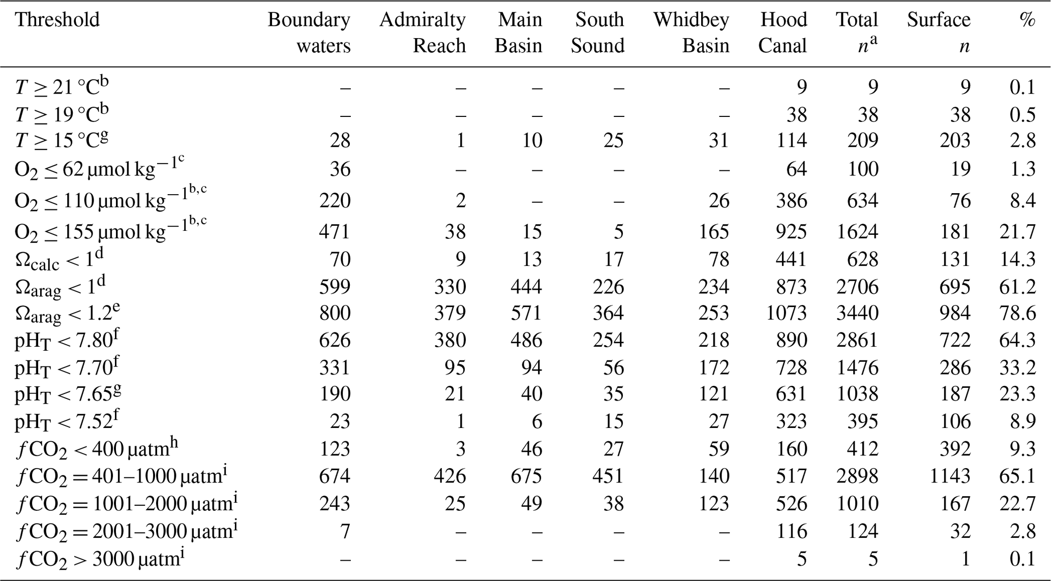
^a Total numbers of data points in the Salish cruise data package are 7526 for temperature, 7492 for oxygen, and 4449 for inorganic carbon measurements. ^b Migration blockages for adult salmonids occur at 19–23 °C, particularly in combination with oxygen levels below 3.5 mg L⁻¹ (∼ 110 µmol kg⁻¹) to 5 mg L⁻¹ (∼ 155 µmol kg⁻¹) (McCullough et al., 2001; U.S. Environmental Protection Agency, 2003). ^c Thresholds for sublethal to lethal hypoxia impacts range from 0.7–2.5 mg L⁻¹ for various invertebrate taxa to 1.5–4.4 mg L⁻¹ for fish (Vaquer-Sunyer and Duarte, 2008); the threshold of 2.0 mg L⁻¹ is commonly used to delineate hypoxic conditions (∼ 62 µmol kg⁻¹ = 1.4 mL L⁻¹), with 0.7 mg L⁻¹ (∼ 31 µmol kg⁻¹ = 0.5 mL L⁻¹) as a threshold used for “severe hypoxia” in the oceanographic literature (e.g., Grantham et al., 2004; Chan et al., 2008). ^d Thermodynamic saturation threshold for calcium carbonate saturation states (e.g., Zeebe and Wolf-Gladrow, 2001; Dickson et al., 2007). ^e Represents severe dissolution and growth exposure thresholds for calcifying pteropods (14 d at Ω_arag=1.20 and 7 d at Ω_arag=1.15, respectively; Bednaršek et al., 2019). ^f Decapod sensitivity thresholds from Bednaršek et al. (2021b), as described in the text. ^g A multi-stressor vulnerability analysis specific to Dungeness crab used temperature, oxygen, and pH_T thresholds of 15 °C, 62 µmol kg⁻¹, and 7.65, respectively, after testing a range of values for each parameter (Berger et al., 2021). ^h The 400 µatm fCO₂ value represents the approximate atmospheric CO₂ mole fraction (xCO₂) during 2008–2018 (the range of mean annual global marine boundary layer atmospheric xCO₂ across 2008–2018 is 385–408 ppm, per NOAA Global Monitoring Laboratory, 2022). Below atmospheric levels, uptake of atmospheric CO₂ by surface water air–sea exchange is favored; above atmospheric levels, outgassing or evasion from surface waters to the atmosphere is favored. Values of xCO₂ are ∼ 2.5 % higher and pCO₂ values are ∼ 0.4 % higher than fCO₂ at seawater surface atmospheric pressure and are different as a result of considering relative humidity and molecular interactions within the measured sample (Dickson et al., 2007). ⁱ fCO₂ levels above atmospheric values have been divided into broad bins based on thresholds used in the literature to project hypercapnia impacts in fish and invertebrates (McNeil and Sasse, 2016) and behavioral to gene expression responses observed in Pacific salmon (Williams et al., 2019).

5.2 Biogeochemical anomalies during 2014–2018

When the atmospheric and marine heatwaves that warmed the Salish Sea surface and deep waters began, a simplistic expectation would have been that increased temperatures would drive increased rates of respiration in deep waters, assuming an adequate supply of organic matter. If a temperature-driven increase in respiration had dominated, we would have expected to see lower-than-normal O₂ and Ω and higher fCO₂ in deep water masses during high temperature anomalies. In contrast, either surface warming or stronger-than-normal freshwater input could have limited primary production by cutting off the surface nutrient supply under stronger stratification, resulting in reduced supply of organic matter and higher-than-normal O₂ and Ω and lower fCO₂ at depth. Additionally, input of NE Pacific source waters at depth with a stronger surface water signal (due to the reduced deep mixing during the MHW) may have also contributed to the higher O₂ and Ω and lower fCO₂ at depth. However, biogeochemical anomalies observed in this time series did not show a simple temperature-dependent response to the heat anomaly; rather, they reflected a combination of heat and river discharge influences.

5.2.1 Hypoxia anomalies

We know from observations and models that hypoxia often occurs in hotspots further south than Salish cruise stations on the Washington shelf during late summer (Connolly et al., 2010; Peterson et al., 2013; Siedlecki et al., 2015, 2016b; Barth et al., 2024), and the resulting hypoxic water masses can be advected northward into our study area (Mickett and Newton in PSEMP Marine Waters Workgroup, 2018). Deep boundary water anomalies observed during the heat anomaly were the opposite of the temperature-driven expectation, with a more-oxygenated water column during O14 than earlier cruises this time of year (cf. Au08, O11, and S13 in Fig. 4 in Alin et al., 2024). Fall boundary water cruises after O14 never captured hypoxic waters in JdFC and measured hypoxic conditions at one shelf station during O17, although deep waters were closer to the hypoxia threshold in O17 and O18 than in O14 and O16. The presence of deep, well-oxygenated water to greater depths than normal in boundary waters during O14 is consistent with the advection of fresher, warmed, well-oxygenated water from the NE Pacific gyre that moved onshore and dominated the upper water column during 2014–2015 (Siedlecki et al., 2016a; Peterson et al., 2017).

Hypoxic conditions were not observed in MB in this cruise time series or in moored near-bottom time series (Fig. 9 in Alin et al., 2024, and https://nwem.apl.washington.edu/prod_PS_ClimateTrends.shtml, last access: 20 March 2024, respectively), likely due to the degree of mixing and shorter residence times (e.g., Babson et al., 2006; MacCready et al., 2021). Minimum deep O₂ values in MB during S15 and S18 were somewhat higher than during pre-MHW fall cruises, whereas they were slightly lower in S16 and S17. Surface O₂ levels were particularly high in MB during A17 and J17 and, to a lesser extent, in A16 and J16 (Fig. 6, Table 4, and Fig. 9 in Alin et al., 2024). In combination with observations of sustained MB phytoplankton blooms during April–August 2017 (PSEMP Marine Waters Workgroup, 2018), these high surface O₂ anomalies suggest that high phytoplankton biomass during spring of 2016 and spring–summer 2017 provided stronger inputs of organic matter to deep MB waters in both years, resulting in lower O₂ levels due to enhanced respiration at depth by the fall of each year.

In contrast, deep HC waters develop hypoxia during some years, typically in August–September in southern HC (Feely et al., 2010; Newton et al., 2011). Hypoxic water masses were observed during the O11 and S14 cruises in the process of being circulated out of the deep southern HC basin by the fall marine intrusion (Fig. 9 in Alin et al., 2024). The O₂ content in HC deep water was not exceptionally low in S14 compared with earlier hypoxia years. However, during continued higher temperatures through 2015–2016, anomalously low O₂ conditions in deep southern HC waters were apparent as early as April of both years (compared with A17, A18, and https://nwem.apl.washington.edu/prod_PS_ClimateTrends.shtml, last access: 20 March 2024) and worsened considerably by J15 and J16. The most extensive and severe hypoxic conditions captured in southern HC during the 2008–2018 Salish cruise time series were observed during the J15 and J16 MHW cruises (Fig. 6, Table 2). Unexpectedly, by S15 and S16, deep-water O₂ minima were higher than in J15 and J16 as well as during the S14, S17, and S18 cruises. In 2015 and 2016, early marine intrusions flushed out deep waters and improved conditions sufficiently by September so that smaller volumes of low-O₂ water remained compared with during a relatively good pre-MHW year (cf. S09 in Fig. 9 in Alin et al., 2024; references in Table 1). In contrast, the S17 and S18 O₂ levels in deep HC water reflected hypoxic conditions equivalent to a bad pre-MHW year, with respect to both timing and magnitude.

5.2.2 Acidification anomalies

Late-summer–early-fall fCO₂ values in surface boundary waters ranged from <400 to >800 µatm in surface waters before the heat anomaly, with waters below 100–150 m consistently >1200 µatm (Fig. S4). Comparable pre-MHW Ω_arag values spanned ∼ 1 to >2, with the lowest deep values being <0.6 (Au08, O11, S13 in Figs. 8 and S4). During O14 and particularly in O16, smaller volumes of >1200 µatm water and the deepest aragonite saturation horizon (depth where Ω_arag=1) were observed in boundary waters. These observations are consistent with NE Pacific source waters with a lower respiration signal having been advected to the Washington coast and persisting in the water column to significant depth during late 2014–2016 (cf. Franco et al., 2021). In contrast, the highest fCO₂ values measured in boundary waters to date were observed during O17, from coastal to AR stations, with fCO₂ extremes of >1600 and >2400 µatm measured at the surface and at depth, respectively. Contemporaneous Ω_arag values were ∼ 0.35, corresponding to Ω_calc values <0.6 and pH_T values <7.3 (Figs. S7, S8). While these values are not unprecedented within PS, they had not been observed previously in these boundary waters or the northern CCE.

Summer and fall cruises in 2014–2018 showed most surface fCO₂ observations <600 µatm throughout MB, SS, and AR, with spatially limited surface areas below atmospheric saturation levels (∼ 400 µatm CO₂), and most of the water column having >800 µatm fCO₂ by the month of September (Fig. S5). While the lowest Ω_arag values typically co-occur with hypoxia, Ω_arag values fell below the thermodynamic threshold (Ω_arag=1) at most times and places in PS, whereas the occurrence of hypoxic conditions was typically limited to a few months per year in southern HC (Figs. 9, S6; Table 3). In MB, surface conditions during S14 were similar to conditions in Au08, whereas during S15 and S16, surface Ω_arag conditions were somewhat lower, but bottom waters had fewer low Ω_arag measurements. In contrast, MB surface waters had larger volumes of low-CO₂ water than usual in A17 and J17, corresponding to the particularly high O₂ observations and reflecting a protracted MB bloom (PSEMP Marine Waters Workgroup, 2018). These lower fCO₂ conditions were followed by unprecedented high fCO₂ and low Ω_arag observations throughout the water column in MB during S17 (Figs. 8–9, S5–S6; Table 2).

HC fCO₂ and Ω_arag temporal dynamics roughly followed the trajectory described for O₂. The most harmful pre-MHW conditions were observed during S09 and O11, with comparable extreme values during S14 (Figs. S5–S7). More severe and widespread fCO₂ and Ω_arag conditions occurred during J15 and (to a lesser extent) J16, with fCO₂ values up to 3460 µatm, Ω_arag as low as 0.23 (Ω_calc=0.36), pH down to 7.13, and O₂ reaching 12 µmol kg⁻¹ (Table 2). High fCO₂ values in S17 were similarly severe but less widespread than in J15, and S18 conditions were as widespread but less severe than S09, which had the most widespread pre-MHW high fCO₂ values. The 12 fCO₂ observations higher than the pre-MHW record came from the J15 and S17 cruises. Relationships between Ω values and O₂ content in HC (R²>0.7) indicate that aragonite and calcite saturation thresholds (i.e., Ω_arag=1 and Ω_calc=1) occur at O₂ levels of 225 and 145 µmol kg⁻¹, respectively, indicating that even calcite undersaturation occurs more frequently and is more widespread than hypoxia within the southern Salish Sea. The early, extreme J15 fCO₂ and Ω_arag conditions in HC were likely caused by heatwave-driven subsurface respiration. In contrast, the elevated S17 conditions appear to reflect spring–summer runoff anomalies that strengthened stratification and early seasonal blooms, which in turn would have enhanced deep respiration. Notably, the lowest fCO₂ minima across the global surface CO₂ observing network have been observed in HC during early spring and the highest maxima have been observed in fall–winter (Alin et al. in PSEMP Marine Waters Workgroup, 2021; cf. Sutton et al., 2018).

5.2.3 Implications of hydrological anomalies for future biogeochemistry in the southern Salish Sea

While the most severe biogeochemical conditions observed in the Salish Sea through 2018 occurred in J15 and J16, coincident with the maximum expression of the MHW in PS, the biogeochemical response to higher temperatures was not simple with respect to driving the observed low-O₂, low-Ω_arag, high-fCO₂ conditions. Rather, the indirect effects of increased temperature on biogeochemistry via the impacts of regional atmospheric warming and precipitation anomalies on watershed hydrology (e.g., river discharge volume and timing) and circulation (stratification and deep-water renewal timing) proved to be equally important in shaping the observed biogeochemical anomalies. Prior results have shown that drought as well as enhanced runoff can exert strong influence on circulation and oceanographic conditions in the Salish Sea (Newton et al., 2003, and references in Table 1). The combination of increased atmospheric heat during most of 2013–2018, as well as record-setting precipitation anomalies and earlier snowmelt in the region, caused earlier and higher river discharges that appear to have enhanced estuarine circulation earlier in the year, resulting in bottom water renewal earlier in 2015 and 2016 than is typical. In this case, while HC bottom waters were more hypoxic, corrosive (low Ω), and high in CO₂ in J15 and J16, conditions in the deep basin had improved by S15 and S16 as a result of these early flushing events.

An independent example of the importance of hydrology to regional biogeochemical conditions came in 2017, the sole year with a normal annual air temperature between 2013 and 2018. High river discharge in spring delivered nutrient and stratification conditions suitable for unusually protracted phytoplankton blooms in MB and left a fresher salinity signature that persisted until September (Table 2). The blooms led to high surface O₂ and Ω_arag and low fCO₂ conditions in MB during spring–summer 2017 but were translated to unprecedented high-fCO₂, low-Ω_arag conditions through the water column by S17 as a result of the subsequent respiration of the high spring–summer phytoplankton biomass. However, while fCO₂ and Ω_arag experienced striking anomalies in 2017 compared with 2016 or 2018, deep MB O₂ levels in S17 were unexpectedly slightly higher than in S16 or S18, presumably because the water column started the growing season more oxygenated at depth in A17 than during A16 or A18 (Fig. 9 in Alin et al., 2024). HC also experienced some of its most extreme fCO₂ and Ω_arag conditions during S17, indicating that runoff-enhanced biological processes were likely stimulated across PS basins; however, the conditions were less obviously anomalous in HC where hypoxia and extremely acidified conditions are known to recur. This interpretation is consistent with numerical simulation results indicating that freshwater inflow and estuarine exchange anomalies exerted a stronger influence on the biomass of primary producers in the Salish Sea than increased heat associated with the 2014–2016 heat anomaly (Khangaonkar et al., 2021).

The strongest biogeochemical anomaly seen in the boundary waters was the high fCO₂ and low Ω_arag values observed throughout the SJdF water column the following month (O17). Comparing observations across October cruises indicates that O₂ minima were also higher in O17 than in O16 or O18 in SJdF, while O17 fCO₂ maxima and Ω_arag minima were substantially higher and lower, respectively, than observed in O16 or O18. In fact, oxygen concentrations at a southern HC location known for hypoxia were described as “the least hypoxic on record over the last several years” (Ruef et al. in PSEMP Marine Waters Workgroup, 2018). Extreme acidified conditions during O17 in SJdF thus showed the same pattern as in MB: not particularly low O₂ levels compared to either O16 or O18 co-occurring with fCO₂ and Ω_arag values completely outside the range of previous observations (Table 2). Widespread low-O₂ and low-Ω_arag conditions are known to have occurred during summer 2017 on the Washington shelf (Olympic Coast National Marine Sanctuary and Simone R. Alin, unpublished data). The driver of these shelf conditions could have been higher coastal productivity and respiration, although no pronounced coastal anomalies in temperature, salinity, or upwelling were observed during Salish cruises earlier in 2017 to support this interpretation (Figs. 2–4, S4; Table 1). However, lower coastal salinities at depth suggest a potential role of anomalous river input in coastal hypoxia in 2017 as well (Mickett and Newton in PSEMP Marine Waters Workgroup, 2018). It remains unclear whether the strongly acidified water mass in SJdF in O17 was the same acidified water mass observed in MB and SS during S17, subsequently circulated out of PS via estuarine circulation, or the acidified shelf water mass observed in unpublished data. Either way, the acidified conditions were likely distributed throughout the SJdF water column by a downwelling wind event that occurred during or just before the O17 cruise.

Because 2017 revealed an anomaly during which O₂ and CO₂ dynamics were decoupled, manifesting as strong acidification not accompanied by particularly low-oxygen or marine heatwave conditions, we dubbed this novel biogeochemical anomaly a “CO₂ storm”, because it was characterized by particularly high fCO₂, and accompanied by low Ω_arag, Ω_calc, and pH_T. The “storm” terminology follows from the description of “carbonate weather” by Waldbusser and Salisbury (2014). Notably, we observed these CO₂ storm conditions in September 2017 in PS's MB (Figs. 8b, 9b, S5–S8) and October 2017 in SJdF (Figs. 8a, 9a, S4), which are locations not previously identified as acidification or hypoxia hotspots. With the higher level of background acidification in HC, what appears to be a CO₂ storm in other basins may manifest as less-anomalous carbonate weather there, much as a rainstorm appears less unexpected in a rainforest than a desert. The background acidification and hypoxia gradient across the region – low in MB, moderate in SJdF, and high in HC – thus afforded us the opportunity to observe novel biogeochemical responses to environmental anomalies.

Collectively, the environmental anomalies of 2013–2018 yielded distinct types of biogeochemical anomalies in the Salish Sea. Marine heat anomalies may drive coupled O₂ and CO₂ system anomalies, whereas terrestrial runoff anomalies driven by atmospheric heat or precipitation anomalies can lead to decoupled O₂ and CO₂ anomalies, as shown here. To understand how future CO₂ storms may affect estuarine and coastal organisms and ecosystems, it is critical to have coupled O₂ and CO₂ system observations because a proxy approach to estimating carbonate chemistry from O₂ and physical parameters will not accurately predict CO₂ storm conditions (e.g., Juranek et al., 2009; Alin et al., 2012). For organisms with sensitivity to high-CO₂ or low-Ω or pH conditions, direct observation of extreme CO₂ events like those described here would be the only way to know that these anomalous conditions had occurred, which may in turn provide insight for interpreting observed ecological changes (e.g., changes in abundance of sensitive species or onset of a marine disease outbreak). Further, maintaining and enhancing these coupled observations will improve the ability of coupled 3D physical–biogeochemical ocean simulations, such as Regional Ocean Modeling System (ROMS) models, to better differentiate and attribute the roles of and complex interactions among atmospheric, terrestrial, and marine processes in influencing estuarine and coastal acidification (Khangaonkar et al., 2021).

6 Biological importance of understanding changing conditions in the Salish Sea and its boundary waters

The iconic marine biota of the Salish Sea – Pacific salmon, Dungeness crab, and shellfish – are important resources supporting the cultural well-being, livelihoods, and food security of Pacific Northwest communities. Many regional species are vulnerable to the direct effects of hypoxic and acidified conditions that naturally occur in this region but are worsening due to climate change. Pink and coho salmon experience changes in their response to olfactory signals that may impair appropriate predator-avoidance behavior during freshwater and early ocean life phases under elevated CO₂ conditions that are currently found in some Salish Sea marine environments (Ou et al., 2015; Williams et al., 2019). Chinook salmon are sensitive to warming temperatures and hypoxia (Crozier et al., 2019, 2021) and may be sensitive to direct ocean acidification impacts as well.

Dungeness crab are the US West Coast's most economically important marine species (e.g., Alin et al., 2015) and an important recreational and tribal fishery in PS (e.g., Froehlich et al., 2017). Recent closures of the Dungeness crab fishery in HC and SS have limited regional access to this marine resource (e.g., Washington Department of Fish and Wildlife, 2020). Field studies show that early life stages experience sublethal dissolution damage to carapaces and mechanoreceptors with sensory and behavioral functions under current conditions (Bednaršek et al., 2020b). Further, Dungeness crab are sensitive to increased temperature and declining oxygen and pH across life stages, with population-level vulnerability to projected warming, hypoxia, and acidification levels from surface to benthic habitats predicted by the year 2100 (Hodgson et al., 2016; Berger et al., 2021). Pacific oysters, another regionally important commercial shellfish species, show a high proportion of defects in larval shell development (Waldbusser et al., 2015) in response to the aragonite saturation levels currently present at most times, depths, and places in PS (Fig. 9, Table 3).

Warming, hypoxia, and acidification also affect the prey and predators for these important species via trophic linkages. Euphausiids (krill) are a dominant food source for finfish and seabirds in the CCE whose larval development and survival are impaired under current pH conditions (McLaskey et al., 2016). Pteropods are another abundant prey source (Bednaršek et al., 2019, and references therein), and calcifying pteropods in the Salish Sea showed severe dissolution effects during 2014–2016 (Bednaršek et al., 2021a). Pteropods experience synergistic effects of high temperature (>11 °C), low oxygen, and low Ω_arag or high pCO₂ on their abundance, shell dissolution, and oxidative stress biomarkers (Bednaršek et al., 2018, 2021a; Engström-Öst et al., 2019). Even the regional apex predator, Southern resident orca whales, whose population has been in decline for decades, may be affected if their dominant food source, Chinook salmon, declines further in abundance as a result of increasingly stressful multi-stressor conditions in the region (Hanson et al., 2021).

Many of the oceanographic variables in this observational data package passed thresholds known to be potentially harmful to regionally important species. Below, we briefly describe the frequencies at which individual and multiple stressors pass known biological thresholds for salmon, crab, and pteropods in order to provide insight to marine resource managers about present-day ecosystem conditions facing Salish Sea resources. These examples of the potential combined biological impacts of ocean acidification, hypoxia, and warming in the Salish Sea illustrate how a complex ecosystem like PS manifests as a mosaic of environmental stressors occurring at different frequencies through space and time.

6.1 Species' thresholds to and occurrence frequencies of individual stressors

Thermal barriers to Pacific Northwest salmonid migration are known to occur at temperatures of 19–23 °C (McCullough et al., 2001). During most July 2014–2018 cruises in HC, temperatures ≥19 °C were observed in the upper 10 m of the water column, with several exceeding 21 °C (Table 3). These observations comprise 0.5 % and 0.1 % of the compiled Salish cruise data product, respectively, and occurred only in HC, although July temperatures also approached stressful levels for salmon in WB. Dungeness crabs have substantial hatch mortality at temperatures >15 °C (Rasmuson, 2013). Temperatures crossed this threshold in 2.8 % of observations, across all basins and dominantly in the upper 20 m, where brooding females aggregate (Pauley et al., 1989; Rasmuson, 2013).

Oxygen levels harmful to salmonids can be as high as 3.5–5 mg L⁻¹ (∼ 110–155 µmol kg⁻¹) (e.g., Table 3 in U.S. Environmental Protection Agency, 2003, and references therein). Oxygen levels ≤ 155 µmol kg⁻¹ comprised 21.7 % of Salish cruise observations (Table 3). Dungeness crab experience feeding cessation in adults at 62 µmol kg⁻¹ (Rasmuson, 2013). Oxygen fell below this hypoxia threshold in 1.3 % of observations, at depths of 5–335 m on both pre- and post-MHW cruises, with a majority at HC stations and 20 % in surface waters. Hypoxic bottom waters in HC have also been shown to drive Dungeness crab to shallower habitats, which may affect their catchability, predation, competition, and cannibalism, and thus potentially future population numbers (Froehlich et al., 2014, 2017). The remaining hypoxic measurements in SJdF and coastal waters (Table 2) do not represent the southern Washington coastal waters where the frequency and severity of hypoxic conditions during the upwelling season is higher (Connolly et al., 2010; Peterson et al., 2013).

As noted previously, aragonite and calcite fall below their saturation thresholds at higher O₂ levels, so the frequencies at which Ω_arag and Ω_calc undersaturation occur are much higher than hypoxia. Ω_arag was undersaturated in 61 % of observations and Ω_calc was undersaturated in 14 % of observations (Table 2), including hundreds of surface observations (Table 3). Biological thresholds for severe dissolution or growth in calcifying pteropods (Ω_arag = 1.15–1.20; Bednaršek et al., 2019) are higher than the thermodynamic threshold, thus yielding > 78 % of all Salish cruise observations below this threshold, of which 33 % were in surface waters. While Ω_arag and Ω_calc thresholds were crossed in all seasons and basins within our study area, the threshold exceedance frequencies are much higher for calcite in HC than elsewhere and much higher for aragonite across all basins than for calcite, temperature, or oxygen conditions becoming harmful.

Increases in fCO₂ levels may affect regionally important species through hypercapnia – the metabolic challenge of too much CO₂ rather than too little O₂. A 1000 µatm pCO₂ threshold for hypercapnia has been used for a range of fish and invertebrate studies (McNeil and Sasse, 2016), although fCO₂ exposure thresholds are not well established for regionally important species. Using the 1000 µatm threshold, >25 % of Salish cruise observations represent conditions potentially conducive to hypercapnia, making them more prevalent than even the 155 µmol kg⁻¹ oxygen threshold for salmon (cf. U.S. Environmental Protection Agency, 2003; Vaquer-Sunyer and Duarte, 2008). While a discrete threshold was not identified for these changes, behavioral, neural, and gene expression responses have been observed in ocean-phase Pacific salmon between treatment pCO₂ levels of 700 and 2700 µatm (Williams et al., 2019). A total of 65 % of Salish cruise CO₂ observations are higher than 700 µatm and 0.4 % are higher than 2700 µatm, implying that ocean-phase Pacific salmon may encounter challenging CO₂ levels in the present-day southern Salish Sea.

A synthesis of decapod species' sensitivity to ocean acidification identified pH_T thresholds of 7.80 for egg hatching success, 7.70–7.74 for adult respiration and hemolymph pH, and 7.52 for larval survival (Bednaršek et al., 2021b, and references therein). Within the Salish cruise data, 9 %–64 % of pH_T observations crossed these thresholds, with pH conditions below the larval mortality threshold occupying much of the water column in HC during summer–fall (Fig. S8, Table 3). Broader pH_T survival threshold estimates for larval, juvenile, and adult decapod life stages span 7.40–7.80 (Bednaršek et al., 2021b); these thresholds were crossed at <10 % to >60 % frequencies in the Salish cruise data. A multi-stressor vulnerability analysis on Washington and Oregon coastal Dungeness crab populations used a pH_T=7.65 threshold across life stages to assess exposure levels under present and future conditions (Hodgson et al., 2016; Berger et al., 2021); a total of >23 % of Salish cruise observations exceeded this threshold. Dungeness thresholds for pH_T sensitivity were crossed with the highest frequency and severity in HC (Fig. S8). This chronic exposure in subsurface HC may be sublethal (Berger et al., 2021, and references therein), but the effects of acidified conditions on population distributions and crab catchability during Washington's tribal and state fisheries is currently unknown (cf. Froehlich et al., 2017).

6.2 Co-occurrence or interactions of multiple stressors in the present-day southern Salish Sea

Populations of valuable Pacific salmon and trout, including some classified as “Threatened” under the US Endangered Species Act, have their native habitat in PS and its watersheds (NOAA Fisheries, 2022). The combination of high temperature and low oxygen can be particularly disruptive for salmonid migration. Temperatures ≥ 19 °C never co-occurred in the same sample with O₂ ≤ 155 µmol kg⁻¹. However, a 21.8 °C temperature occurred at 2.7 m depth with O₂ levels of 99.6 µmol kg⁻¹ and fCO₂ levels of 1437 µatm at 10.9 m at the same HC station during J18, putting three known salmon stressors in close physical proximity, with the risk of combined physiological effects and habitat compression (Table 4). Similar combinations of temperature, oxygen, and fCO₂ conditions were also recorded during J16 and J17 in southern HC. Several salmonid runs enter a nearby river for the metabolically challenging breeding migration during summer, when these conditions formed near the river mouth (Generalized Life History and Life Stage Incidence by Month for the Skokomish River Salmonid Populations, Skokomish Tribe, Skokomish Nation, Washington, Cindy Gray, personal communication, 2022). If heatwave conditions observed during summer 2015 are representative of the future marine stressor landscape, harmful levels of temperature, oxygen, and fCO₂ may be more likely to co-occur earlier in the salmon run season, rather than occurring separately, with peak temperatures in July and minimum O₂/peak fCO₂ values occurring in September, as was typical during pre-MHW years.

Closer inspection of when and where harmful conditions co-develop in the region reveals that low pH_T and O₂ co-occurred at 23 stations across 10 cruises, with 4 cruises and 15 of the stations sampled prior to the onset of strong, recurring atmospheric and surface water temperature anomalies beginning in 2013 (Tables 1, 4). Of cruises with co-occurring low O₂ and pH, 14 stations were in HC and 9 in boundary waters, and these conditions predominantly affected the bottom waters that juvenile and adult Dungeness crabs inhabit. In contrast, the combination of stressfully warm surface temperatures with low pH_T close below was observed mostly after the onset of heat and other anomalies and during cruises from July into October. This combination occurred during 11 cruises at 61 stations – occupying a wider geographical distribution across PS and boundary waters – with 10 stations in August 2008 being the only cruise prior to September 2013 showing this combination of stressors (Table 4). While these conditions are unlikely to occur in the present day during Dungeness hatching season (winter–spring), anomalously low salinity (<15) can also prevent egg hatching, interfere with larval progression, and be lethal for adults (Pauley et al., 1989; Rasmuson, 2013). Thus, nearshore hatching habitats may have been affected by the major 2013–2018 precipitation and river runoff anomalies (Table 1), providing another example of how hydrological anomalies may have profound ecosystem effects in PS, beyond effects on carbonate chemistry. We note that low salinity anomalies should also be considered to be part of the multi-stressor management landscape.

A triad of Dungeness crab stressors – high temperature (> 15 °C), low O₂ (<62 µmol kg⁻¹), and low pH_T (<7.65) (Berger et al., 2021) – co-occurred six times at stations in southern HC during the J15, J16, and S17 cruises (Table 4). Stressful conditions for Dungeness spanned much or all of the water column at five stations during the J15 and J16 cruises and occupied the surface and a less extensive part of the subsurface water column during S17. This newly observed co-occurrence of all three crab stressors in HC during 2015–2017 reveals a possible future path for how the multi-stressor marine environment will evolve in this region under warmer climate conditions. Potential biological ramifications include the disappearance of suitable habitat for all life stages of Dungeness crab from some areas of the southern Salish Sea during the pelagic larval and settlement seasons. Summer crabbing seasons across 2008–2019 in HC typically spanned July–August (Hood Canal Recreational Crab – Open fishing days 1995–2021, Washington Department of Fish and Wildlife, Washington, Don Velasquez, personal communication, 2022), making it likely that habitat compression due to combined T, pH, and O₂ stress affected crab depth distributions during this time series and may warrant management consideration. However, parsing whether the combined effects of multiple interacting stressors across crab life stages and habitats have contributed to recent PS Dungeness fisheries closures would require a more complex modeling analysis like those done in coastal waters (Hodgson et al., 2016; Berger et al., 2021).

Table 4 Multi-stressor events relevant to Dungeness crab as well as their temporal and spatial occurrence in the Salish cruise data package. Thresholds to determine event occurrence were those used by Berger et al. (2021). Depth ranges affected by combinations of hypoxic (oxygen content <62 µmol kg⁻¹), low-pH_T (pH_T < 7.65), or high-temperature (>15 °C) conditions are indicated in the “Depth range” columns. Cruises that occurred before the beginning of major atmospheric and surface seawater temperature anomalies in the summer of 2013 are shown using italic font.

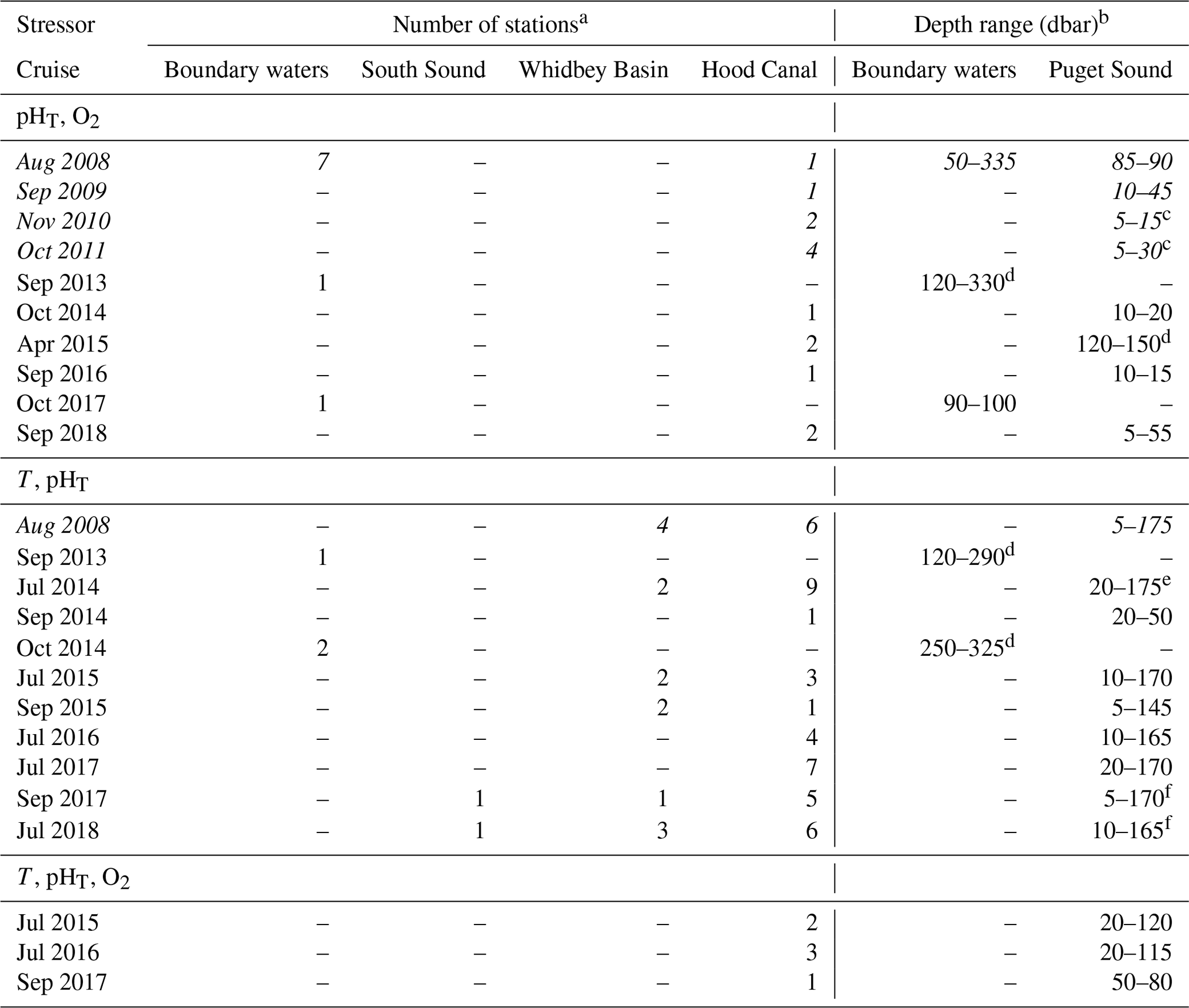
^a Multiple stressors never occurred at a single station simultaneously in Main Basin or Admiralty Reach, so they are not included in this table. ^b Depth ranges affected by pH_T or O₂ threshold exceedance are rounded to the most inclusive 5 dbar intervals, although the sampling resolution was sparse enough that the depth ranges affected by low-pH_T or low-O₂ conditions may have been larger for any given cruise. ^c The depths at which hypoxic and low-pH conditions were seen on these cruises were near the surface, not near the bottom; bottom conditions were less harmful. ^d Depth ranges affected were deeper than habitats in which Dungeness crab are typically most abundant on the Washington coast (e.g., Berger et al., 2021). ^e The largest number of stations affected by two independent stressors were observed during this cruise. ^f Combined temperature and pH_T stressor conditions were the most widespread across basins during these cruises.

7 Conclusions: what we have learned about multi-stressor dynamics from the Salish cruise time series so far

Ocean acidification variables indicate stressful conditions throughout the region, although with substantial regional variation. Aragonite undersaturation was pervasive throughout the region, and even calcite undersaturation occurred more widely and frequently than hypoxia. fCO₂ levels were above atmospheric values in >90 % of observations, often by hundreds of microatmospheres. Hypoxia was observed most frequently in southern HC and occasionally in boundary waters during 2008–2018. This seasonally resolved cruise time series co-occurred with several major environmental anomalies, giving us the opportunity to observe the impacts of atmospheric and marine heatwaves, precipitation, and river discharge anomalies on Salish Sea physical and biogeochemical conditions. The strongest heat anomalies manifested earlier in boundary water cruises (October 2014) but in a delayed and more protracted way within PS, spanning at least 2015–2016. Increased temperatures throughout the water column likely contributed to the most extreme O₂, fCO₂, and Ω_arag conditions seen in southern HC during July 2015 and July 2016, developing earlier in the season than the typical late-summer timing for previous hypoxia events. However, anomalously early deep-water renewal events in HC in 2015 and 2016 resulted in late-summer conditions that resembled a less-hypoxic, pre-heatwave year in deep southern HC. The effects of the heat anomaly thus underscore the importance of physical oceanographic conditions (i.e., temperature, stratification, and circulation timing) in setting the stage for the severity and duration of ocean acidification and hypoxia in local hotspots.

Both seasonal and spatial variation was strong. The decade-long Salish cruise time series illuminated several differences in the seasonality across parameters and across PS and its boundary waters. Some parameters peaked at the surface during summer (temperature and Ω_arag), with others rising (salinity and fCO₂) or falling (O₂) from spring to fall, while all parameters showed more monotonic seasonal progression at depth. Within PS, the largest overall variability was observed in the most stratified basins. Notably, deep-water seasonality in HC was different from other basins in that seasonal O₂ lows and highs co-occurred with temperature and salinity minima and maxima, whereas salinity and temperature were inversely correlated with O₂ content in other basins. The lags likely result from the combination of more complex deep-water renewal and earlier spring blooms in HC, which appear to decouple its physical and biogeochemical seasonality relative to other deep PS basins and may predispose it to more hypoxic, acidified conditions. To the extent that climate change alters the coupling between physical and biogeochemical seasonality in other regional waters, changes in the frequency, severity, and duration of ocean acidification and hypoxia may be expected.

During fall 2017, we observed a novel carbonate system anomaly in PS and boundary waters. This CO₂ storm was characterized by unprecedented high fCO₂ and low Ω_arag values, which crossed sensitivity thresholds for regionally important species. This extreme event occurred independently of heatwave or particularly low oxygen conditions and instead appears to have resulted from major river discharge anomalies reflected by low salinity anomalies observed earlier in the year. The CO₂ storm was most obvious in basins with less-acidified baseline conditions but was still detectable in the most acidified basin, HC. These observations showed decoupling of carbonate chemistry from that of oxygen, which was unusual in this time series. This result underscores the need for ongoing seasonal monitoring of both carbon and oxygen across Salish Sea basins, which showed variable responses to anomalies in physical ocean conditions, river input, and local weather. The Salish cruise time series has thus illustrated how the arc of major environmental anomalies and their ecological impacts depends on the biogeochemical metric, species of interest, and baseline conditions of the basins in which they occur.

The frequencies at which Salish cruise observations crossed known or preliminary species' sensitivity thresholds illustrate the relative risk landscape of temperature, hypoxia, and acidification anomalies in the southern Salish Sea in the present day. Interactions between marine heat and other environmental anomalies during the 2014–2018 cruises revealed how multiple stressors can combine to present potential migration, survival, or physiological challenges to key regional species. Collectively, the occurrence frequencies of these combinations of stressors for Dungeness crab, salmon, and pteropods in the Salish cruise data package illustrate how increasingly frequent and severe marine and atmospheric heatwaves may alter the future co-occurrence of multiple stressors in the southern Salish Sea. Specifically, while low pH_T and O₂ co-occurred regularly before the heat anomalies in mostly subsurface HC and boundary waters, the co-occurrence of high-surface-temperature and low-pH conditions appeared to increase sharply across the marine heatwave, with a broader spatial distribution than where low pH and O₂ previously co-occurred. Future changes in the seasonality of when harmful conditions develop and co-occur may cause sensitive species' thresholds to be crossed more frequently due to changes in timing, even without changes in severity. The novel forms and combinations of extreme events observed in the 2014–2018 Salish cruise time series have, thus, provided insight into the potential evolution of the future marine stressor risk landscape in the Salish Sea.

In summary, observing assets deployed throughout coastal and estuarine environments in this region allowed us to detect unexpected biogeochemical anomalies in this region, including decoupling between hypoxia and acidification conditions, that would not have been discovered without high-quality measurements of both oxygen and carbonate system variables. The ability of 3D ocean simulations to accurately project complex ecosystem multi-stressor events and their impacts on marine species will benefit from comparison with rich observational data sets such as this cruise time series, which is capable of resolving seasonal events throughout the water column and diverse basins of the southern Salish Sea. Further synthesis of the rich information from this data product alongside that from the moored time series in this region, with its relatively high temporal resolution (sub-daily), may facilitate increased understanding of mechanisms driving variation, which is needed to further develop recommendations for multi-stressor monitoring approaches and analyses.