the Creative Commons Attribution 4.0 License.
the Creative Commons Attribution 4.0 License.
 | 26 Apr 2024
Validation of the coupled physical–biogeochemical ocean model NEMO–SCOBI for the North Sea–Baltic Sea system
Itzel Ruvalcaba Baroni
Elin Almroth-Rosell
Lars Axell
Sam T. Fredriksson
Jenny Hieronymus
Magnus Hieronymus
Sandra-Esther Brunnabend
Matthias Gröger
Ivan Kuznetsov
Filippa Fransner
Robinson Hordoir
Saeed Falahat
Lars Arneborg
The North Sea and the Baltic Sea still experience eutrophication and deoxygenation despite large international efforts to mitigate such environmental problems. Due to the highly different oceanographic frameworks of the two seas, existing modelling efforts have mainly focused on only one of the respective seas, making it difficult to study interbasin exchange of mass and energy. Here, we present NEMO–SCOBI, an ocean model (NEMO-Nordic) coupled to the Swedish Coastal and Ocean Biogeochemical model (SCOBI), that covers the North Sea, the Skagerrak–Kattegat transition zone and the Baltic Sea. We address its validity to further investigate biogeochemical changes in the North Sea–Baltic Sea system. The model reproduces the long-term temporal trends, the temporal variability, the yearly averages and the general spatial distribution of all of the assessed biogeochemical parameters. It is particularly suitable for use in future multi-stressor studies, such as the evaluation of combined climate and nutrient forcing scenarios. In particular, the model performance is best for oxygen and phosphate concentrations. However, there are important differences between model results and observations with respect to chlorophyll a and nitrate in coastal areas of the southeastern North Sea, the Skagerrak–Kattegat transition zone, the Gulf of Riga, the Gulf of Finland and the Gulf of Bothnia. These are partially linked to different local processes and biogeochemical forcing that lead to a general overestimation of nitrate. Our model results are validated for individual areas that are in agreement with policy management assessment areas, thereby providing added value with respect to better contributing to international programmes aiming to reduce eutrophication in the North Sea–Baltic Sea system.
- Article
(24244 KB) - Full-text XML
- BibTeX
- EndNote


The North Sea and the Baltic Sea share similar ecological problems, such as eutrophication and deoxygenation (e.g. Peeters et al., 1995; Rönnberg and Bonsdorff, 2004; Greenwood et al., 2010; Gustafsson et al., 2012; Große et al., 2016; Andersen et al., 2017), despite being two substantially different basins. They differ from each other with respect to bathymetry, geometry and, forcing conditions, which control their ocean dynamics and, thus, lead to two fundamentally different turnover timescales. The area between the two seas, hereafter referred to as the Skagerrak–Kattegat transition zone, includes several subbasins (Fig. 1) and is the only connection between the Baltic Sea and Atlantic waters. This zone is also one of the most heavily anthropogenically impacted areas of the North Sea–Baltic Sea system (e.g. Korpinen et al., 2013; Kenny et al., 2017); therefore, it is relevant to include the region in ecological assessment studies for both seas. Previous biogeochemical studies (both based on both modelling and observations) in the Skagerrak–Kattegat transition zone have focused on nutrient fluxes, eutrophication, summer algal blooms and primary production, although with a primary focus on the Kattegat for the period between 1950 and 2000. These studies concluded that there was a decline in phosphorus and bottom oxygen concentrations after ∼ 1980 (Andersson, 1996; Rasmussen and Gustafsson, 2003); that primary productivity increased until at least the year 1980, after which the trends are less clear (Carstensen and Conley, 2004; Rydberg et al., 2006); and that important nutrient gradients exist within the Kattegat (Danielsson et al., 2004).
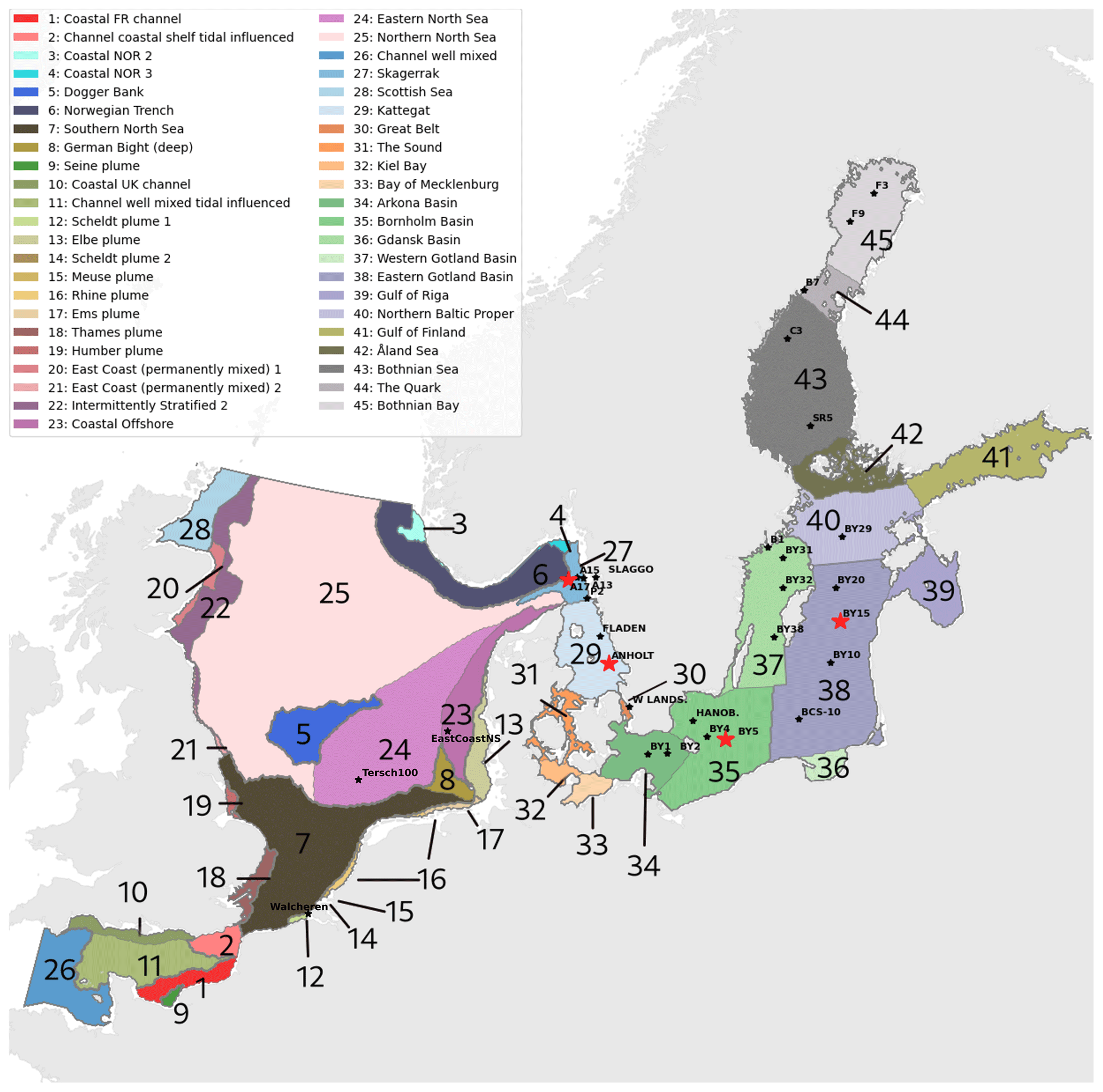
Figure 1Combined division of assessment areas from COMP4 OSPAR 2021 (1 to 28) and Baltic Sea assessment units from HELCOM 2021 (29 to 45) adapted to our model domain. Note that the HELCOM division is shown for the Kattegat, whereas the OSPAR division is shown for the Skagerrak. Stars represent the analysed stations. The stations shown in this study are highlighted in red. The bathymetry of the domain is shown in Hordoir et al. (2019).
The Baltic Sea is a landlocked sea with several subbasins separated by sills. It is shallow, with an average depth of only about 53 m, but it encompasses the Gotland Deep (∼ 249 m) and the Landsort Deep (∼ 459 m) in the eastern and western Gotland Basin, respectively (e.g. Jakobsson et al., 2019). It has brackish water with both a north-to-south salinity gradient and a strong perennial stratification in all deep basins. In the shallow areas, winds are capable of mixing the entire water column down to the seafloor, whereas the deeper basins have a permanent strong halocline. In the central Baltic Sea, horizontal advection of saline water below the permanent halocline can occur (Reissmann et al., 2009). The stratification is due to a large freshwater input from rivers at the surface and the advection of dense, salty, oxygenated waters to deeper layers from the North Sea that enter through the Danish straits and spread across the Baltic Sea basins (e.g. Stigebrandt, 1987; Döös et al., 2004; Leppäranta and Myrberg, 2009). However, this stratification also inhibits the supply of oxygen to deep waters via vertical mixing. Thus, oxygen transport to deep waters occurs mainly via intermittent inflows of saline water through the Danish straits, primarily during the winter at irregular (annual to multiyear) intervals (e.g. Gustafsson, 1997; Omstedt et al., 2004; Lass and Matthäus, 1996; Feistel et al., 2008; Hordoir et al., 2015). This strong stratification also promotes a homogeneous distribution of biogeochemical properties and a long water mass residence time (ca. 35 years) (Döös et al., 2004; Wulff et al., 2001; Meier and Kauker, 2003; Feistel et al., 2008). Primary productivity in the Baltic Sea is mainly limited by nitrate, which favours the growth of nitrogen-fixing cyanobacteria (e.g. Granéli et al., 1990; Janssen et al., 2004; Eilola et al., 2009; Kuliński et al., 2022).
Contrary to the Baltic Sea, the North Sea is much more dynamic, with a residence time of only a few years (Otto et al., 1990; Hordoir et al., 2019), and it is heavily influenced by tides. Consequently, it is generally well mixed and well oxygenated, but its deeper areas are periodically stratified. Deoxygenation can occur in coastal and stratified areas of the eastern North Sea, primarily when influenced by riverine input (Devlin et al., 2022; van Leeuwen et al., 2023). Tidal mixing fronts occur between deep stratified and tidally mixed shallow waters (e.g. Ikeda et al., 1989; McGlade, 2002; Ducrotoy et al., 2000; Sündermann and Pohlmann, 2011). About 53 % of the North Sea is permanently, seasonally or intermittently stratified (van Leeuwen et al., 2015). While nutrients have been identified as the main factor controlling primary productivity in the North Sea, other factors, such as temperature, stratification and light penetration depth, have a regional impact (e.g. Holt et al., 2012; Ly et al., 2014; Burson et al., 2016). Its ocean dynamics and biogeochemistry are also greatly influenced by the adjacent open Atlantic Ocean (e.g. Winther and Johannessen, 2006; Gröger et al., 2013; Mathis et al., 2019; Huthnance et al., 2022).
Diatoms and flagellates, which are adapted to a wide range of salinity conditions, can dominate the primary production in both seas. More specifically, in the Baltic Sea, diatoms have been found to dominate stations with the highest salinities, whereas flagellates and other autotrophs were most abundant at low-salinity stations (Olofsson et al., 2020a). In the North Sea, tidal mixing fronts favour the growth of diatoms (e.g. Ikeda et al., 1989; McGlade, 2002; Ducrotoy et al., 2000; Sündermann and Pohlmann, 2011), while stratified waters favour the growth of flagellates (e.g. van Leeuwen et al., 2015). However, their spatial distribution and total biomass in both seas may vary significantly from year to year and from subbasin to subbasin (e.g. Henriksen, 2009; Reid et al., 1990; Ford et al., 2017; Olofsson et al., 2020a). In contrast, filamentous cyanobacteria (hereafter referred to cyanobacteria) do not tolerate high-salinity conditions (e.g. Mazur-Marzec et al., 2005; Olofsson et al., 2020b) and, therefore, do not grow in the North Sea. However, they are key in the brackish Baltic Sea, where they can dominate the (late-)summer primary production (e.g. Finni et al., 2001; Janssen et al., 2004; Olofsson et al., 2020b).
The entire North Sea–Baltic Sea system has experienced increased anthropogenic nutrient loads from rivers, the atmosphere and point sources (i.e. any single identifiable source of pollution from which pollutants or nutrients are discharged, such as sewage) since the early 1900s and especially after the 1950s (e.g. Savchuk et al., 2008; Vermaat et al., 2008; Gustafsson et al., 2012; Holt et al., 2012). This has led to an acceleration of algal growth (i.e. eutrophication), especially in coastal waters, and oxygen deficiency in bottom waters. In particular, (late-)summer cyanobacteria blooms occur in the Baltic Proper, which have been found to be closely linked to the variability in the phosphorus supply to surface waters and stratification and to changing redox conditions in the water column (Kahru et al., 2000; Janssen et al., 2004; Eilola et al., 2009). Because of the different renewal timescales, the nutrients are recycled much faster in the North Sea than in the Baltic Sea. However, neither the North Sea nor the Baltic Sea have yet fully recovered despite large efforts to reduce nutrient loads since the 1980s to 1990s. In the North Sea, persistent eutrophication has been linked to a stronger reduction in phosphorus versus nitrogen loads, which have created nutrient imbalances that affect the growth and species composition of marine phytoplankton communities (Burson et al., 2016; Ly et al., 2014). In the Baltic Sea, the slow recovery is linked to the fact that the water column nutrient inventory is tightly coupled to that of the sediments due to the long and frequent exposure to low-oxygen conditions. This accelerates the recycling of phosphorus from sediments under deoxygenated bottom waters (e.g. Koop et al., 1990; Mort et al., 2010; Jilbert and Slomp, 2013).
Studies on the ecological and geopolitical status of the North Sea and the Baltic Sea have highlighted the need for more long-term monitoring data and improved models to support the Marine Strategy Directives and international programmes aiming to improve ecological conditions in the North Sea–Baltic Sea system (Ducrotoy and Elliott, 2008; Mee et al., 2008; Koho et al., 2021). Indeed, several European Union management programmes and directives are now well established (e.g. OSPAR, 2003; Borja, 2006; HELCOM, 2006) and can, as part of a challenging but possible joint effort, cover the whole of the North Sea and the Baltic Sea (Koho et al., 2021). In respective studies by Almroth and Skogen (2010) and Eilola et al. (2011b), the eutrophication status of the North Sea–Baltic Sea system for the year 2005 and the years 2001–2006 was assessed based on observations and ensemble model results. However, none of the models used in these studies included both seas; instead, they combined results from several models to analyse the entire North Sea–Baltic Sea system. Covering both seas in one single model is a big advantage, as it avoids the need to formulate reasonable lateral boundary conditions, often based on a limited number of observations that may oversimplify the actual dynamics. This can greatly influence the model results, which is particularly true in the Skagerrak–Kattegat transition zone. To our knowledge, only two other 3D ocean models with fully coupled biogeochemistry cover both the North Sea and the Baltic Sea (Daewel and Schrum, 2013; Maar et al., 2011). Their results show generally good agreement with observations in time and space, but they contain biases for different biogeochemical parameters. Thus, large model uncertainties still exist for the North Sea–Baltic Sea system, linked to differences in model set-ups and process descriptions. Having a variety of independent models for similar domains is important to assess such uncertainties (Eilola et al., 2011a).
In the present study, we use the NEMO-Nordic (Hordoir et al., 2019) ocean model with a model domain covering both the North Sea and the Baltic Sea and, for the first time, couple it to the Swedish Coastal and Ocean Biogeochemical model (SCOBI). The latter has previously been used in many applications for the Baltic Sea (e.g. Almroth-Rosell et al., 2015; Eilola et al., 2009, 2012; Meier et al., 2012) and the Swedish coast (Edman et al., 2018). We present the model results and model skill compared to observational-based estimations. We also link our analysis to the latest policy management areas agreed upon in the fourth application of the Comprehensive Procedure (COMP4) within the Oslo–Paris Commission (OSPAR) for North Atlantic waters and the North Sea and the Helsinki Commission (HELCOM) for the Baltic Sea (Fig. 1) to identify regional model performance and to, in the future, better contribute to European initiatives on the de-eutrophication of both the North Sea and the Baltic Sea.
2.1 Model description
We use the coupled physical–biogeochemical NEMO–SCOBI ocean model, in which the ocean component is based on the Nucleus for European Modelling of the Ocean (NEMO) framework (Madec et al., 2017), version 3.6. This 3D model has been specifically configured for the Baltic Sea and the North Sea (NEMO-Nordic; Hordoir et al., 2015, 2019) by the Swedish Meteorological and Hydrological Institute (SMHI) and covers an area from 4.15278° W to 30.1802° E and from 48.4917 to 65.8914° N (Fig. 1). The biogeochemistry is simulated by SCOBI, which has also been developed at SMHI (Marmefelt et al., 1999; Eilola et al., 2009; Meier et al., 2012; Eilola et al., 2012; Almroth-Rosell et al., 2015). The SCOBI model has been successfully coupled to different ocean and coastal models (e.g. Almroth-Rosell et al., 2011; Edman et al., 2018); however, previous model domains only cover either the Baltic Sea, including the Kattegat, or Swedish coastal waters. Here, for the first time, the SCOBI model is coupled to NEMO-Nordic and, therefore, computes changes in key biogeochemical properties in the water and sediments for the entire NEMO-Nordic domain. The ocean model coupled to the biogeochemistry is referred to as NEMO–SCOBI.
In the present study, the model was integrated from 1961 to 2017 and validated for recent years (2001–2017), as biogeochemical observations are more abundant after the year 2000. The period before 1975 is regarded as a spin-up. For the physics, we use all settings as in Hordoir et al. (2019) but with an updated physical forcing and representation of fast ice, allowing it to form only in shallow areas when attached to the shore (Siiriä et al., 2022). We also use daily river forcing instead of monthly. The physical and biogeochemical settings are described in Sect. 2.1.3 and 2.1.4, respectively.
2.1.1 Ocean hydrodynamic model: NEMO-Nordic
NEMO-Nordic has a regular grid with 56 vertical levels with a resolution of 3 m close to the surface, decreasing to 22 m at the bottom of the deepest part of the domain (Norwegian Trench), and a horizontal resolution of approximately 2 nmi (∼ 3.7 km). NEMO-Nordic has two open boundaries: a meridional one, located in the western English Channel between Brittany and Cornwall, and a zonal one, located between Scotland and Norway (Fig. 1). For further details on ice and ocean dynamics, the reader is referred to Pemberton et al. (2017) and Hordoir et al. (2019), respectively.
2.1.2 Biogeochemical model: SCOBI
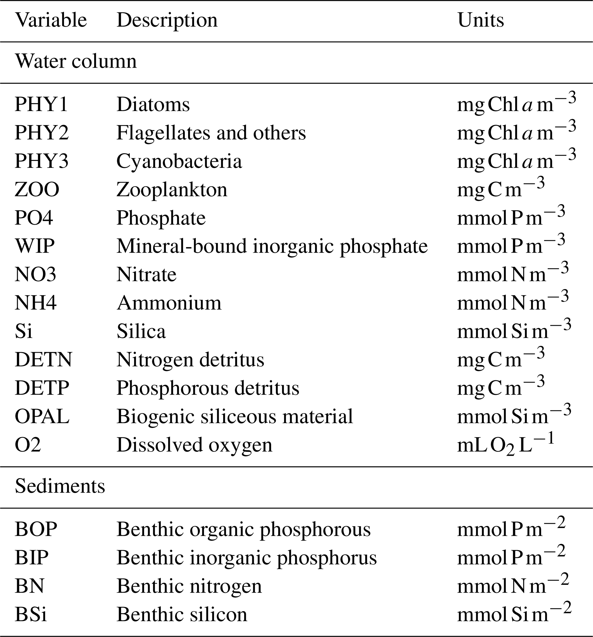
The SCOBI model (first described by Marmefelt et al., 1999) is a process-oriented nutrient, phytoplankton, zooplankton, and detritus (NPZD) model that traditionally simulated three major marine biogeochemical cycles (nitrogen, phosphorous and oxygen) in both the water column and sediments (Eilola et al., 2009; Almroth-Rosell et al., 2011, 2015). Now coupled to NEMO-Nordic, SCOBI also includes the marine silicon cycle. Currently, the model has 17 biogeochemical state variables, 13 of which are pelagic and 4 of which are benthic. The state variables are summarized in Table 1, and a diagram summarizing the biogeochemical cycling in SCOBI is shown in Fig. 2. The inorganic forms in the water column are represented by six state variables: dissolved oxygen (O2), nitrate (NO3), ammonia (NH4), phosphate (PO4), mineral-bound inorganic phosphorus (WIP) and dissolved silicate (DSi). Dead particulate organic material in the water column is separated in three variables as detritus: nitrogen detritus (DETN), phosphorus detritus (DETP) and amorphous biogenic silica (OPAL). Nutrients are assimilated by three phytoplankton functional groups defined as diatoms (PHY1), flagellates and others (PHY2), and cyanobacteria (PHY3), which are all grazed by bulk zooplankton (ZOO). In SCOBI, hydrogen sulfide concentrations are represented by “negative oxygen” equivalents so that (in mL O2 L−1) (Fonselius, 1962). The model accounts for one sedimentary layer containing the benthic reservoirs of nitrogen (BN), silicon (BSi), organic phosphorus (BOP) and inorganic phosphorus (BIP), where BIP represents a benthic pool of phosphate adsorbed to mineral particles (e.g. iron oxides) (Almroth-Rosell et al., 2015).
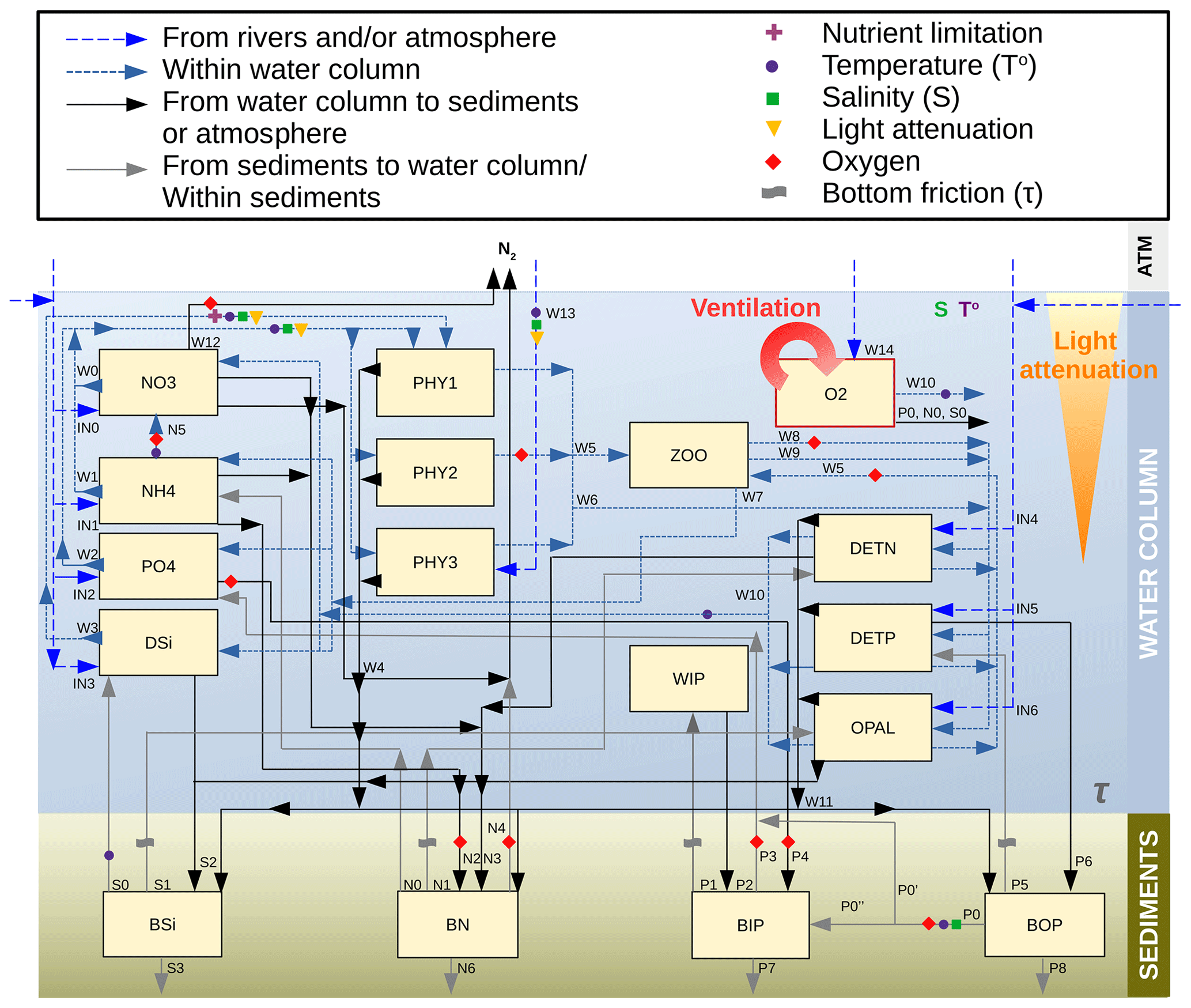
Figure 2Schematics of the biogeochemical processes included in NEMO–SCOBI, where the main variables determining a process (as an independent variable or as a threshold) are indicated with symbols. Processes for plankton, detritus and oxygen are as follows: W0 – nitrate uptake for phytoplankton growth; W1 – ammonium uptake for phytoplankton growth; W2 – phosphate uptake for phytoplankton growth; W3 – silicate uptake for diatoms growth; W4 – sinking and sedimentation of phytoplankton; W5 – grazing; W6 – mortality; W7 – excretion/sloppy feeding; W8 – predation; W9 – zooplankton faeces; W10 – remineralization of detritus and oxygen consumption; W11 – sinking and sedimentation of detritus; W12 – water column denitrification; W13 – N2 fixation by cyanobacteria; and W14 – oxygen exchange between the atmosphere and surface water. Processes for phosphate are as follows: P0 – phosphate release from the decomposition of organic matter in sediments (P0′ – the fraction of the mineralized benthic organic phosphorus that is directly released to the overlying water; P0′′ – the fraction that is transferred to the benthic inorganic phosphorus); P1 – resuspension of inorganic phosphorus; P2 – deposition of inorganic phosphorus; P3 – phosphate release from benthic inorganic phosphorus; P4 – scavenging of phosphorus into sediments under oxic conditions; P5 – resuspension of organic phosphorus; P6 – deposition of organic phosphorus; P7 – burial of inorganic phosphorus; and P8 – burial of organic phosphorus. Processes for nitrogen are as follows: N0 – nitrogen release from decomposition of organic matter in sediments (N0′ – the fraction released as nitrate; N0′′ – the fraction released as ammonium); N1 – resuspension of organic nitrogen; N2 – ammonium adsorption to particles; N3 – deposition of organic nitrogen; and N4 – total benthic denitrification (which consists of two pathways – denitrification of pelagic nitrate and denitrification of benthic nitrogen); N5 – water column nitrification; and N6 – burial of organic and inorganic nitrogen. Processes for silica are as follows: S0 – silicon release of benthic silicon; S1 – resuspension of benthic silicon; S2 – deposition of silicon; and S3 – burial of organic and inorganic silicon. Input fluxes from rivers are for nitrate, ammonium, phosphate, silica and detritus for both phosphorus and nitrogen (IN0 to IN5). Atmospheric inputs are for all nutrients except silica, which is only supplied by rivers.
The main processes included in the water column are primary production, N2 fixation, grazing and sloppy feeding, remineralization of organic matter and its resulting oxygen consumption, sinking of particles, nitrification, denitrification, and organic matter deposition to the sediments. Within the sediments, dissolved nutrients can be released back to the water column due to the remineralization of organic matter, and deposited organic material can be resuspended back to the water column due to currents and wave bottom friction. Under oxic conditions, a fraction of the phosphate from remineralized benthic organic phosphorus adds to the benthic pool of inorganic phosphorus, whereas the other fraction is released directly to the water column. The sizes of the fractions are oxygen dependent. Moreover, scavenging of phosphorus from the water column takes place, adding to the benthic inorganic phosphorus pool. Under anoxic conditions, all of the remineralized phosphorus is directly released to the water column, as well as a fraction of the benthic pool of inorganic phosphorus. For benthic nitrogen, a fraction of the remineralized nitrogen is removed by benthic denitrification (BDEN). The fraction depends on the available oxygen concentrations in the bottom waters, with a medium rate during oxic conditions and a maximum rate under low-oxygen conditions that decreases rapidly to a null rate during anoxic conditions. However, benthic denitrification can continue when the bottom water is anoxic if nitrate is available in bottom waters, following Eq. (A26) (Appendix A2). The parameterization of the other processes above is described in Eilola et al. (2009), and the latest modifications to the benthic phosphorus are given in Almroth-Rosell et al. (2015). In the SCOBI version coupled to NEMO, rates and dependencies for phytoplankton growth were modified with respect to previous SCOBI versions in order to account for silica limitation of diatoms (not included in earlier versions), improve the occurrence of dominant groups in both the North Sea and the Baltic Sea, and limit cyanobacteria growth in the Skagerrak–Kattegat transition zone and stop their growth in the North Sea. To include benthic processes in the North Sea, new rates of burial and nutrient release from sediments and the resuspension of benthic organic nutrients due to wave and current friction were introduced. In addition, the parameterization of oxygen penetration depth was replaced by the oxygen concentration in bottom waters in benthic redox-dependent processes for phosphorus, as NEMO–SCOBI does not include oxygen in the sediment layer. For clarity, we detail the current SCOBI formulations for phytoplankton growth and all relevant sedimentary processes in Sects. A1 and A2 in Appendix A.
2.1.3 Physical setting
The meteorological forcing is taken from the Uncertainties in Ensembles of Regional ReAnalyses data (UERRA; e.g. Dahlgren et al., 2016, available at https://www.uerra.eu, last access: November 2019) with a spatial resolution of 11 km and a time resolution of 1 h for wind, air pressure, air temperature, humidity, and solar and long-wave downward radiation and a time resolution of 12 h for precipitation (i.e. rain and snow).
The open boundary forcing consists of barotropic currents, sea level and nine tidal constituents as well as monthly salinity and temperature data. The barotropic currents and sea level are calculated using the 2D North Atlantic Model (NOAMOD; She et al., 2007) storm-surge model for 1979–2017. These were corrected for baroclinic effects using monthly sea level data from the European Centre for Medium-Range Weather Forecasts' Ocean Reanalysis System 4 (ORAS4) to improve the ocean circulation in the North Sea. To extend it back in time, we applied a neural-network-based regression technique, following Hieronymus et al. (2019). The salinity and temperature profiles are monthly mean values interpolated from an ORAS4 configuration (Balmaseda et al., 2013).
Daily values of runoff for the period from 1961 to 2019 were provided by a dedicated simulation with the Hydrological Predictions for the Environment model with the European application v.3.1.8 (E-HYPE; Donnelly et al., 2016). Here, these were reduced by a factor of 0.9 based on the best results for salinity in surface waters from a sensitivity analysis performed with NEMO–SCOBI. For more details on the applied river runoff, the reader is referred to Ruvalcaba Baroni et al. (2024). For the physical initial conditions, we used restart files from the simulation in Hordoir et al. (2019) that were the closest to the observations for physical properties at the start of the simulation.
2.1.4 Biogeochemical settings
For the initialization, the biogeochemical initial values are derived from a combination of typical North Sea and Baltic Sea profiles and spin-up values from previous sensitivity tests performed with NEMO–SCOBI. These represent better background physical–biogeochemical conditions than using a homogeneous 3D field in the initialization, and the aforementioned conditions are then further improved by the actual spin-up. The forcing for the open boundary conditions for the biogeochemical model was created based on the International Council for the Exploration of the Sea (ICES) database (Beszczynska-Möller et al., 2009) and interpolated as seasonal cycle climatology to the model grid.
The atmospheric nutrient forcing, consisting of bioavailable nitrate, ammonium and phosphate, and nitrogen detritus, was interpolated as seasonal cycle climatology from yearly averages of total atmospheric loads of nitrogen and phosphorus in the Baltic Sea and period averages reported per basin for 1994–2006 in Savchuk et al. (2012). Here, ammonium, nitrate and detritus are assumed to be 40 %, 50 % and 10 % of the total atmospheric nitrogen load, respectively. A constant value per nutrient per basin and per month is then given to individual model grid cells (in ). While the atmospheric input of both nitrogen and phosphorus increases from 1975 to the 1980s, only nitrogen clearly decreases after the 1980s. The resulting atmospheric input of both total phosphorus and nitrogen to the Baltic Sea is comparable to values reconstructed by Gustafsson et al. (2012) and reported for recent years by HELCOM (Gauss et al., 2022). However, historic nitrogen atmospheric inputs are uncertain, and our method resulted in higher loads (∼ 100 kt N yr−1) than those in Gustafsson et al. (2012) for years before 1995. In the North Sea, historic atmospheric loads are also uncertain, especially those for phosphorus. Here, we use the total atmospheric nutrient load for the Baltic Proper to reconstruct the specific loads in the North Sea, resulting in nitrogen loads that are comparable to those reported by OSPAR for the years 1994–2014 (Bartnicki et al., 2019) but fairly constant values for phosphorus loads after the year 1970.
The daily riverine nutrient loads are based on the dedicated E-HYPE run, which includes a more realistic number of river outlets than those reported in the observational data sets. While the E-HYPE data set captures the interannual variability well, it does not account for the increase in nutrients due to increased fertilizer use in the 1960s and the consequent reduction due to the nutrient regulation policy in the 1980s. Hence, we do not use the river forcing as originally provided. Instead, the riverine nutrient loads were corrected for each year and each basin to the level of compiled observational data for nutrient loads combining two data sets, one for the North Sea (the ICG-EMO database of European rivers; Lenhart et al., 2010) and one for the Baltic Sea (Gustafsson et al., 2012). The result is an E-HYPE forcing with river points adapted to the NEMO-Nordic grid (Fig. 3) and with slightly reduced runoff and modified nutrient loads that include the increase and the following decrease seen in observations (Fig. 4). The latter nutrient forcing is available, described and compared to the former data sets in Ruvalcaba Baroni et al. (2024).
In addition, the detritus loads for nitrogen and phosphorus in the SCOBI model are reduced by a factor of 0.3 for nitrogen and 0.75 for phosphorus once they reach the coastal waters (i.e. the river loads of detritus enter the detritus pool in the SCOBI model as 0.3× river DETN and 0.75× river DETP, respectively). This is to account for only the bioavailable fraction of the organic matter coming from rivers and coastal retention. As the response to nutrient removal of different coastal types is poorly quantified, especially in the North Sea, these factors are taken from previous studies in the Baltic Sea (Eilola et al., 2011a; Edman and Anderson, 2014; Asmala et al., 2017). Because E-HYPE does not include the silica cycle, we use a compilation of observations for both the North Sea and the Baltic Sea adapted to the NEMO-Nordic river points to reconstruct the silica river loads. Two main data sets for silica loads (the Baltic Nest Institute – Stockholm University – personal communication with Bo Gustafsson, 2020; the ICG-EMO database of European rivers – Lenhart et al., 2010) were combined to include as many observation points as possible for both the North Sea and Baltic Sea (not shown).
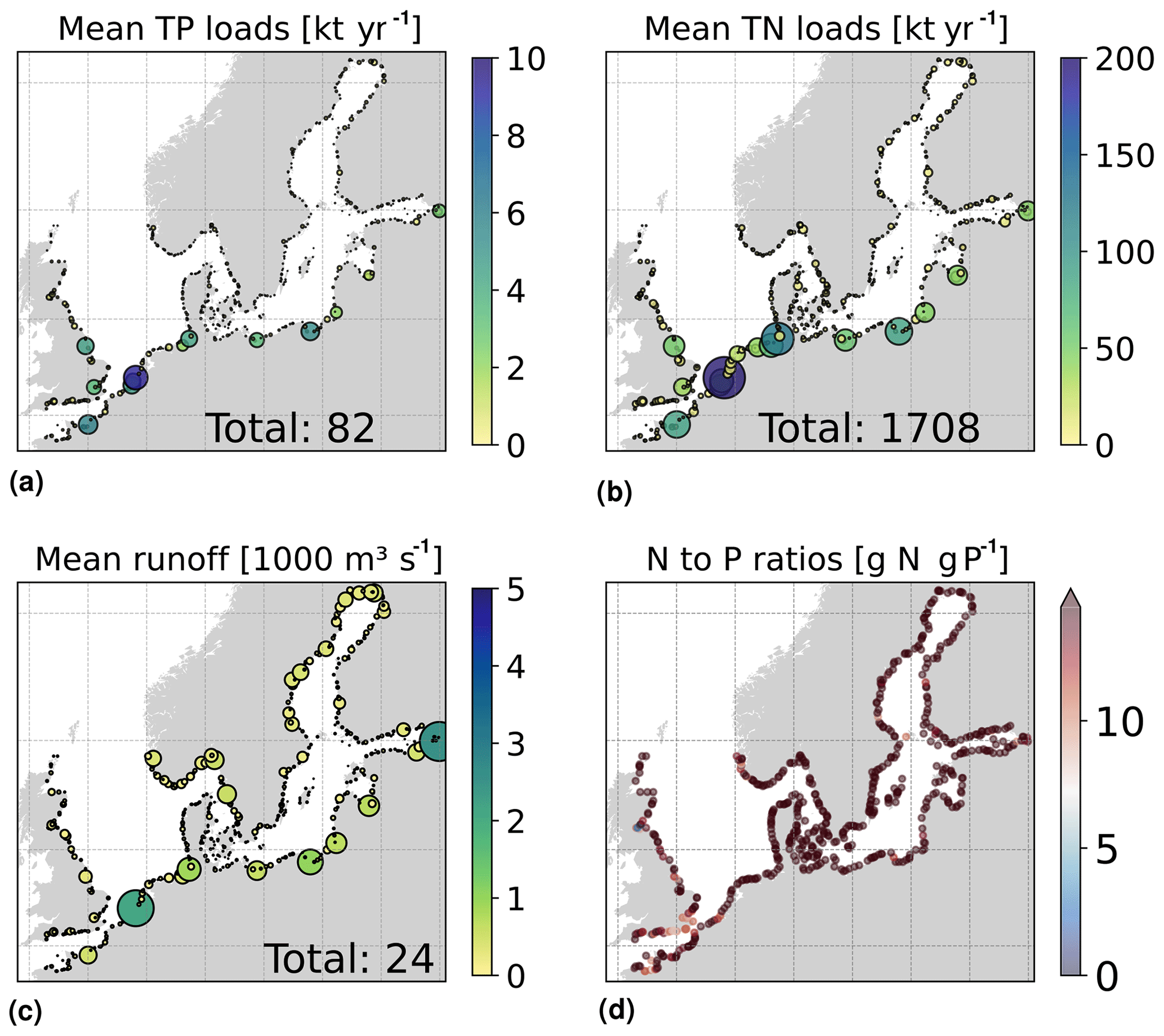
Figure 3Averaged riverine loads of (a) total phosphorus (), (b) total nitrogen () and (c) runoff for the period from 2001 to 2017 in the river forcing applied to the model domain. Circle sizes illustrate the relative load contribution in the area; the total period average for the domain is also shown. Panel (d) shows the nitrogen and phosphorus (N-to-P) ratios for each river point, where the Redfield ratio is ∼ 7 g N (g P)−1.
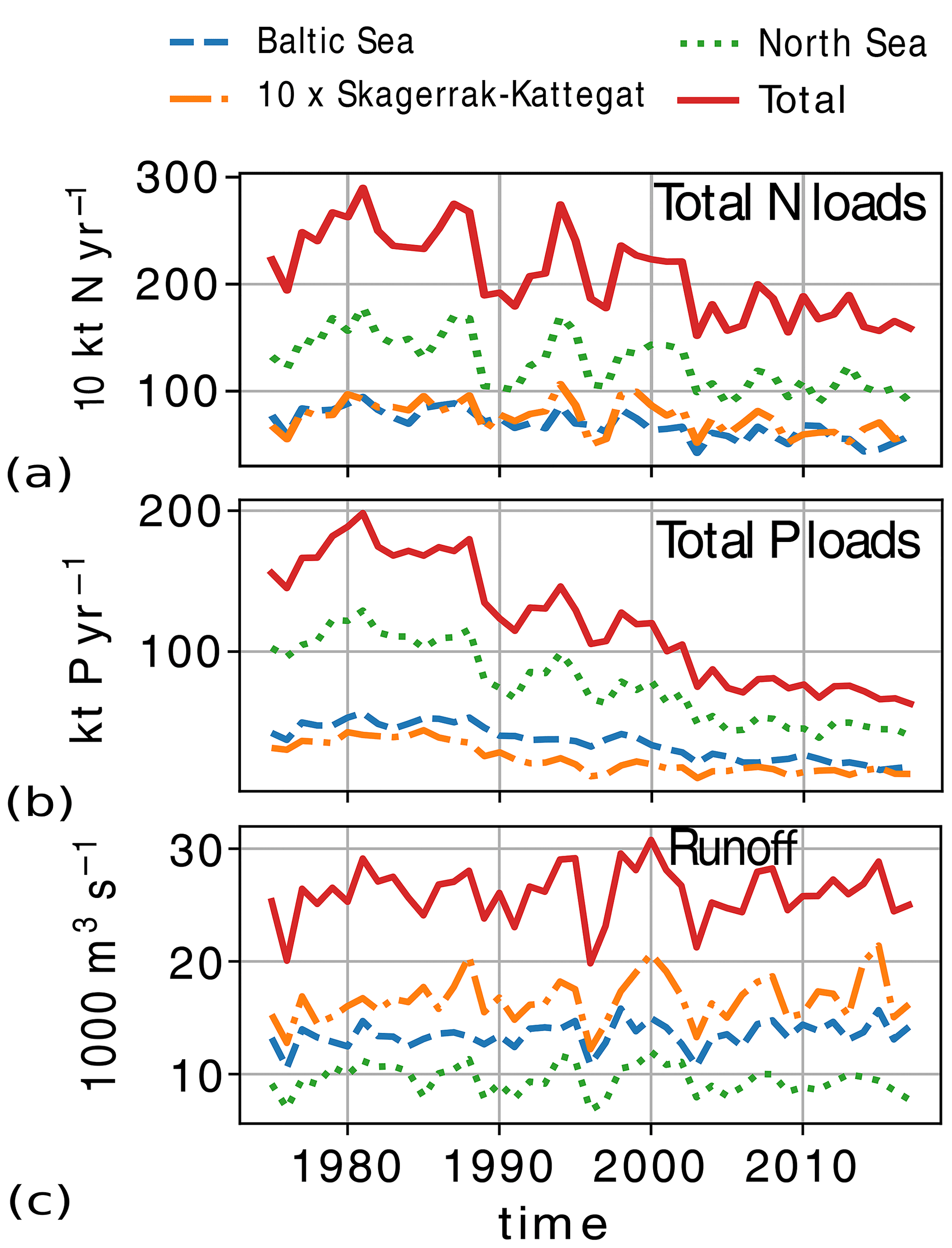
Figure 4Riverine loads of (a) total nitrogen (), (b) total phosphorus () and (c) total runoff from 1975 to 2017 in the model domain and its subbasins: the North Sea, the Skagerrak–Kattegat transition zone and the Baltic Sea. For plotting reasons, numbers for the Skagerrak–Kattegat transition zone are multiplied by 10 here.
2.2 Observations and validation method
In order to compare model results to observations, nitrate, nitrite, ammonium, phosphate, particulate organic nitrogen, particulate organic phosphorus, chlorophyll a, oxygen and hydrogen sulfide as well as seawater temperature and salinity were downloaded from the open SHARKweb database (the Swedish national archive for oceanographic data, hereafter referred to as “SHARK”; https://sharkweb.smhi.se, last access: December 2023) and the ICES database (https://www.ices.dk, last access: December 2023). Observations measured more than once a day were averaged to obtain one daily value. However, both data sets are not homogeneously distributed with respect to time, space or depth. Except at fixed stations, which have a temporal resolution of a maximum of twice a month, most positions in the ICES database are rarely measured more than twice a year.
2.2.1 SHARK database
The observations from the SHARK database were used to analyse long-term model results and their interannual variability at 27 selected stations in the Skagerrak–Kattegat transition zone and in the Baltic Sea (Fig. 1). These stations were selected based on their distribution in relevant subbasins of the Skagerrak–Kattegat area and the Baltic Sea (Fig. 1). All stations are well documented and broadly used in monitoring studies. However, observations for chlorophyll a at discrete depths are lacking at stations B7, C3, F3 and F9. At C3, only observations for phosphate in the water column and for oxygen in bottom waters are available. At B7, nitrate, nitrite and ammonium observations are lacking. The number of observations of nitrate and chlorophyll a available in Skagerrak is also scarce before the year 2000.
Euxinia (i.e. waters with no oxygen but free hydrogen sulfide, H2S) is converted from H2S to negative oxygen equivalents in the same way as in SCOBI (see Sect. 2.1.2). If both oxygen and H2S are present and oxygen concentrations are above the detection limit, we use the oxygen concentration; on the other hand, if oxygen concentrations are below the detection limit, we use the H2S conversion.
Daily time series at selected stations in the model were plotted against observations of phosphate, nitrate plus nitrite, oxygen, discrete chlorophyll a, salinity and temperature for the period from 1975 to 2017. These are compared to model results at several discrete depths at all selected stations. For surface waters, both the model and observations were averaged over the first ∼ 10 m for comparison. For bottom waters, observations within the bottom layer of the model were averaged. The daily time series are also used to evaluate the model skill at selected stations for the main biogeochemical parameters (Sect. 2.2.3).
The salinity, temperature and current fields in the North Sea–Baltic Sea system show large variability on decadal timescales that are superimposed on multi-decadal long-term trends, particularly in the North Sea (Daewel and Schrum, 2017). This variability is not necessarily in phase in all regions. In order to evaluate the interannual variability of the model, we analysed averages for a 17-year period (from 2001 to 2017), so that at least one decadal cycle is included as well as the years with the most observations. Note that several medium to strong inflows to the Baltic Sea occurred within this chosen period, e.g. in 2003 and 2014 (Mohrholz et al., 2015; Mohrholz, 2018). In addition, a simple linear regression analysis is performed for the periods 1975–1996 and 1996–2017 for both observations and the model results to detect differences in long-term trends. The year 1996 has been chosen as a reference year in which nutrients are high in most of the model domain and in the observations, although not necessarily when these values are at their maximum. Therefore, the regression analysis here cannot be used to detect the exact timing of potential changes in trends. If the number of observations is less than 40 within the regression time period, no regression line is plotted. The p values are calculated and evidenced against the null hypothesis, considering a significant trend when p value ≤ 0.05.
Monthly (m), seasonal (s) and period (p) averages as well as their corresponding standard deviations with time are calculated at all depths. Note that seasonal averages for the winter months are considered to be from December to February, the spring months are from March to April, the summer months are from May to August and the autumn months are from September to November. The number of observations for each averaged profile () was calculated as a percentage based on the corresponding total number of days () within the period so that the coverage in percent was ⋅ 100. We take a minimum of 3 to calculate the averages and no interpolation in depth or time was performed. Monthly values and their standard deviation were also averaged over the first ∼ 10 m. We evaluate the model skill at selected stations as described in Sect. 2.2.3.
2.2.2 ICES database
To analyse the spatial variability in surface waters, we use the ICES observations for nitrate plus nitrite, phosphate and chlorophyll a within our model domain. These were seasonally averaged from 2001 to 2017 and over the first ∼ 10 m. The difference between each observation data point and its corresponding model point in surface waters is calculated as Mi−Oi. We also use the ICES database to evaluate the spatio-temporal model skill for the main biogeochemical parameters (Sect. 2.2.3) following the management areas agreed upon in OSPAR for the North Sea and in HELCOM for the Baltic Sea. These area divisions were combined; however, as the area definition from OSPAR and HELCOM in the Kattegat overlap and differ from each other, we use the HELCOM definition for the Kattegat (Fig. 1; HELCOM, 2006; OSPAR, 2022). Oxygen is only evaluated below the surface waters, as the model is mainly controlled by the atmospheric conditions in surface waters, resulting in surface oxygen values close to saturation and, therefore, always in good agreement with observations. The number of observations used per area in this study is illustrated in Fig. 5. Areas with less than 100 observations for all four variables within the period from 2001 to 2017 are not shown. These are areas 3, 10, 14, 19, 20 and 21. In addition, the number of observations of oxygen below surface is also less than 100 in areas 1, 2, 9, 11, 12, 15, 16, 18 and 26. Three stations with the highest number of observations in the southern North Sea (Fig. 1) have also been selected from this data set, but their model skill was not evaluated due to too poor observational coverage (Appendix B): Walcheren (51.55° N, 3.41° E), Tersch100 (54.15° N, 4.3419° E) and EastCoastNS (55.25° N, 7° E).
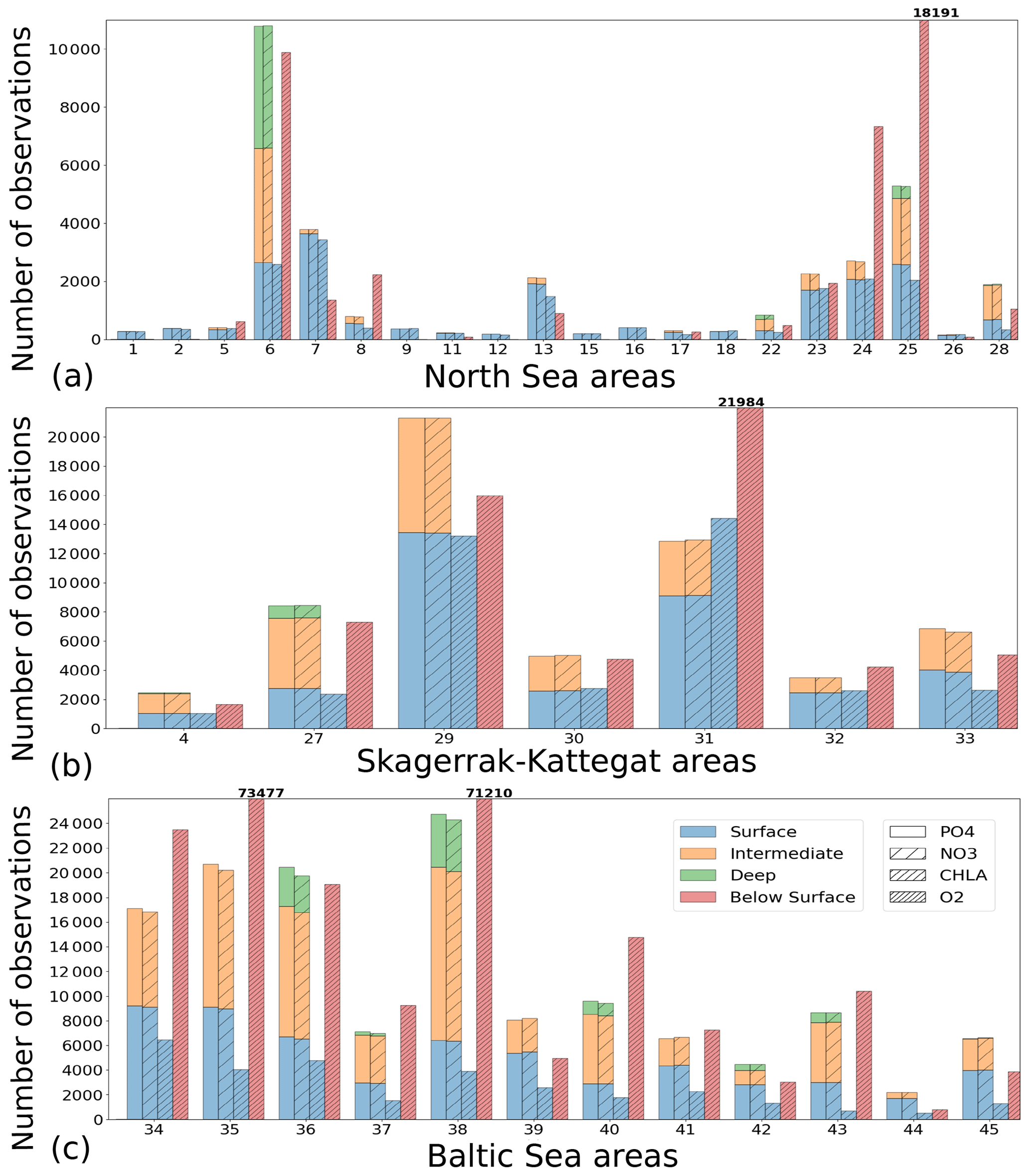
Figure 5Number of observations per area according to Fig. 1 in (a) the North Sea, (b) the Skagerrak–Kattegat transition zone and (c) the Baltic Sea. Observations are for phosphate (PO4), nitrate (NO3), chlorophyll a (CHLA) and oxygen (O2) for the period from 2001 to 2017 in surface (above 10 m), intermediate (between 10 and 100 m) and deep waters (below 100 m). For oxygen, only observations below surface waters are considered (below 10 m). Areas with less than 100 observations for all four variables are not shown (i.e. areas 3, 10, 14, 19, 20 and 21 in the North Sea). Note that the y-axis scales in panels (a), (b) and (c) differ.
2.2.3 Model skill evaluation
To evaluate the model skill, two dimensionless parameters – the Pearson correlation coefficient (r) and the cost function (CF) – are used. Following Eilola et al. (2009), the CF is defined as follows:
where i denotes the point in depth and/or time, n is the number of data points, and M and O are the respective model results and observations. The r value provides information about how well variability in the observations is represented by the variability in the model. The CF gives the proximity of the model to observations by normalizing the bias with the standard deviation (SD) of the observations. While a positive r will always fall between 0 and 1, with 1 being a perfect fit, the CF will only be below 1 when model results fall within the standard deviation of the observations. Similarly to other studies (e.g. Edman et al., 2018; Edman and Anderson, 2014), we combine both skill metrics as 1−r versus CF. Thus, the closer values are to the origin, the better the model performance. More specifically, when values fall within an inner quarter circle with axis (1−r, CF) = (0.33, 1), the model performance is considered to be good. Model values are considered acceptable if they fall outside of this inner quarter circle but within an outer quarter circle with axis (1−r, CF) = (0.66, 2). Large model biases are found when values fall outside the outer quarter circle.
This analysis is performed per station for the period 2001 to 2017 considering all days and depths. We select the stations with a good salinity and temperature model skill to best evaluate the SCOBI performance and, therefore, avoid biases from the ocean model. We also discarded stations with less than 500 observations for this analysis. The period mean and the seasonal model skill for phosphate, nitrate, chlorophyll a and oxygen are then evaluated.
To get an overview of the spatio-temporal performance of NEMO–SCOBI, the model skill for the same biogeochemical parameters is evaluated for the entire domain as a whole and for its subbasins: the Baltic Sea, the Skagerrak–Kattegat transition zone and the North Sea. In order to have an overview at a finer regional scale, a model skill analysis per area was evaluated according to the latest assessment area definitions from HELCOM and OSPAR (Fig. 1). This evaluation is done for the entire water column and for surface, intermediate and bottom waters. Areas with too few observations (<100) for each variable during the period from 2001 to 2017 are not evaluated.
3.1 Validation per station
In general, the long-term trends, the period means and (to a lesser extent) the seasonal cycle of all biogeochemical state variables are well captured by the model at all 27 stations. In addition, the interannual variability in the model is in good agreement with observations at most stations. Each station has local specificities, both with respect to observations and model performance. However, the model performance between stations shows large similarities depending on their proximity to one another. In this section, we present the results of time series for surface and bottom waters as well as averaged-profile analysis from two stations: ANHOLT (Figs. 6, 7) and BY15 (Figs. 8, 9). Here, these are considered to represent the Skagerrak–Kattegat transition zone and the Baltic Proper, respectively. This is because the model response at these two stations is very similar, both with respect to magnitude and trend, to that at stations within their corresponding regions (i.e. the model response at ANHOLT is similar to that at Å13, Å15, Å17, P2, SLÄGGÖ, FLADEN and W LANDSKRONA in the Skagerrak–Kattegat transition zone, and the model response at BY15 is similar to that at BY1, BY2, BY4, BY5, HANÖBUKTEN, BCSIII-10, BY10, BY20, BY29, BY31, BY32 and BY38 in the Baltic Proper). In Sect. B in Appendix B, we also show the results from Å17 (Fig. B1) in the Skagerrak and BY5 (Fig. B2) in the Bornholm Basin (Fig. 1) as further examples. Note that the model response at F9 is similar to that at F3 and C3, representing the Gulf of Bothnia. However, results from this area are not shown due to the lack of observations in this region. Along with the averaged profiles, we show the corresponding observational coverage at all depths, which is never larger than 8 % at all analysed stations (e.g. Figs. 7, 9) and highlights the low temporal resolution of observations (of a maximum of twice a month). Consequently, the probability of missing the monthly maximum (or minimum) in this data set is high; therefore, it may not show the full variability range. Higher-temporal-resolution data sets exist (e.g. Rantajärvi et al., 1998; Greenwood et al., 2010); however, they only cover a few recent years and are not available for all biogeochemical parameters. Therefore, they cannot be used to analyse historic model results. When accounting for long-term time series, the used observational data set becomes more reliable and more likely to be representative of the system. A summary of the regression analysis at ANHOLT and BY15 is listed in Table 2 and plotted together with the time series (Figs. 6, 8).
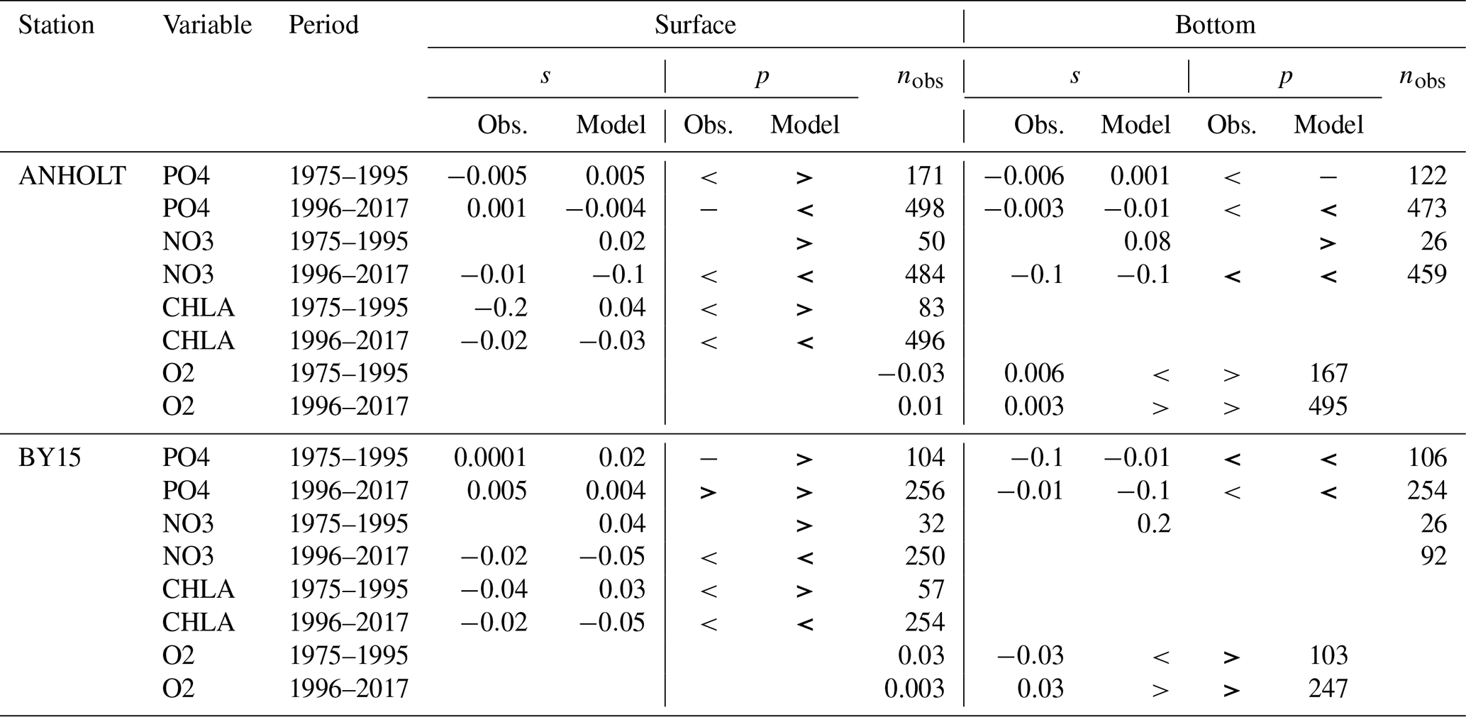
Table 2Summary of both the model and observation trends for the period from 1975 to 1995 and from 1976 to 2017 at ANHOLT and BY15 for phosphate, nitrate, chlorophyll a and oxygen, where the slope (s) and the number of observations (nobs) for surface and bottom waters are shown. The symbols “<”, “>” and “−” denote negative, positive and no trend, respectively. No trend is assumed when . Significant trends – i.e. when p values (p) are ≤0.05 – are indicated in bold.
3.1.1 ANHOLT: Skagerrak–Kattegat transition zone
At ANHOLT, temperature, salinity and oxygen are very well captured by the model, with respect to both time and depth (Fig. 6a, b, f). Phosphate also shows good agreement with observations at all depths, especially in surface waters, where it is fully consumed each year in both observations and the model (Fig. 6c). However, nitrate and chlorophyll a are higher in the model than in the observations (Fig. 6d, e). As in the observations, the modelled nitrate at ANHOLT is depleted in surface waters, but the yearly maxima are too high compared with observations. This results in a period-averaged positive bias of about 5 mmol N m−3 (Fig. 7f). In bottom waters, all model values for nitrate at ANHOLT fall outside of the observation range. Note that the nitrate bias is smaller at all stations in the Skagerrak (e.g. at Å17; Fig. B1 in Appendix B) than those at ANHOLT and FLADEN (not shown) in the Kattegat. Despite this bias, a decreasing nitrate trend after 1995 is seen in bottom waters in both observations and model results (Fig. 6d, Table 2), suggesting that the long-term trend is still captured by the model. The model results show an overall reduction in phosphate in the Skagerrak–Kattegat transition zone for the entire period (i.e. all stations in this region show a negative trend with p values smaller than 0.05 when evaluated for 1975–2017; not shown), in agreement with the findings reported by Rasmussen and Gustafsson (2003) and Wulff and Stigebrandt (1989) after the 1980s in the Kattegat. However, our model results suggest a significant increasing trend from 1975 until the 1990s for surface and bottom nitrate and for surface phosphate at ANHOLT (Fig. 6c, d; Table 2). At ANHOLT, the number of observations before 1996 is too low, especially for nitrate, to be able to validate this trend. However, at the stations in the Skagerrak (Å13 and SLÄGGÖ), where the observational coverage is better, such trends are not observed. In the model results, there is a significant decreasing trend (p value < 0.05) in both nutrients at stations in the Skagerrak after 1996 in both surface and bottom waters, but the trend in surface waters is not statistically significant for observations (p value > 0.05). The model trends in the Skagerrak–Kattegat transition zone are strongly linked to the applied river forcing in this region, which shows an increase in nutrients from the start of the period followed by a decrease after the 1990s (Fig. 4). The poor observational coverage, especially before 1996, makes it difficult to analyse trends in this region only based on observations.
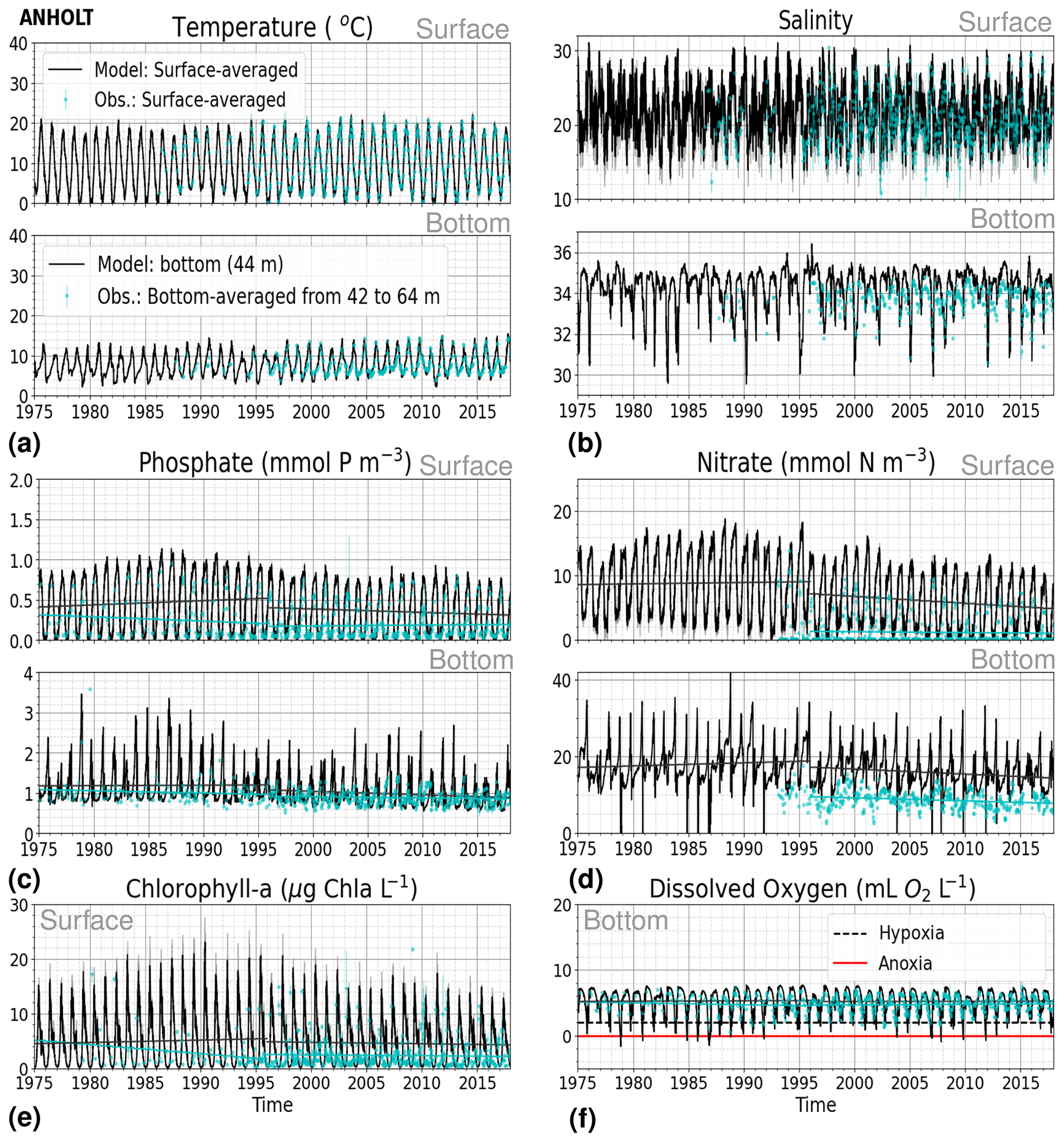
Figure 6Time series of (a) temperature, (b) salinity, (c) phosphate, (d) nitrate, (e) chlorophyll a and (f) bottom oxygen for model results versus observations in surface (averaged over the first ∼ 10 m) and bottom waters for the period from 1975 to 2017 at ANHOLT. A simple linear regression is shown for the 1975–1996 and 1996–2017 periods for both the model results (black) and observations (blue) for phosphate, nitrate, chlorophyll a and oxygen. The standard deviation for surface averages is shown for both the model (grey) and observations (blue). Note that hypoxia and anoxia are considered when oxygen concentrations are below 2 and 0 mL O2 L−1, respectively.
Similarly to findings by Carstensen and Conley (2004), the model shows a small but significant increasing and decreasing trend in chlorophyll a from 1975 to 1996 and towards 2017, respectively. These are not shown by the chlorophyll-a observations, which do not show a statistically significant slope (p value > 0.5) from 1975 to 1996 and towards 2017 (Fig. 6e, Table 2). Observations of chlorophyll a are lacking, especially before the year 1996. In addition, higher maxima of chlorophyll a are more frequently displayed by the model than in the observations. Consequently, the model monthly averages (seasonal cycle climatology) over the period from 2001 to 2017 show higher values than observations (Fig. 7a). Besides the general low temporal resolution in observations, the chlorophyll-a distribution is usually patchy in the Baltic Sea (e.g. Pavelson et al., 1999; Janssen et al., 2004) and, thus, difficult to measure in situ. Hence, these observations represent only a snapshot of nature, and there are no guarantees that the measurements actually capture the chlorophyll peaks; therefore, they may not represent the full amplitude of interannual variability. The monthly averages at ANHOLT show a consistent peak in the observed chlorophyll a in late winter/early spring (February and March) with a later peak in autumn (November), while the model only peaks in May and slowly decreases towards December. Because of this model delay during spring, the seasonal profiles for chlorophyll a, nitrate and phosphate are less well represented by the model at this station, especially for summer (Fig. 7b, e, h). The period-mean nitrate and chlorophyll-a profiles show a consistent positive bias. However, the shape of the seasonal and period-mean profiles are well captured by the model, especially for phosphate.
Even though there are biases in nitrate and chlorophyll a, the monthly, seasonal and mean oxygen profiles are in good agreement with observations (Fig. 7j, k, l). Note that the overestimation of the modelled chlorophyll a above the pycnocline during the summer months is mainly due to the model delay in the phytoplankton growth. A positive oxygen bias of maximum ∼ 2 mL O2 L−1 is, however, observed at ANHOLT in bottom waters, especially for the summer months. This bias is much smaller at all other stations in the Skagerrak–Kattegat transition zone (e.g. Fig. B1j, k, and l in Appendix B). Oxygen concentrations in bottom waters have been suggested to have declined in most basins in the Skagerrak–Kattegat transition zone from 1971 to 1990 (Andersson, 1996). Model results for oxygen concentrations in bottom waters show no clear trends (with small regression slopes) at any Skagerrak–Kattegat transition zone stations (e.g. Fig. 6f, Table 2). In the Skagerrak–Kattegat region, there is a tendency, in both the model and observations, toward an increase in oxygen with time after the 1990s; however, the trend is not statistically significant (p value > 0.05). Thus, a long-term decline in oxygen followed by a recovery is possible in the entire water column and may affect the overall oxygenation in the entire transition zone. In the Skagerrak–Kattegat region (e.g. at ANHOLT; Fig. 6) observational data are largely lacking before the 1990s, including those for oxygen in bottom waters; therefore, model trends may be more representative of the system for historic values.
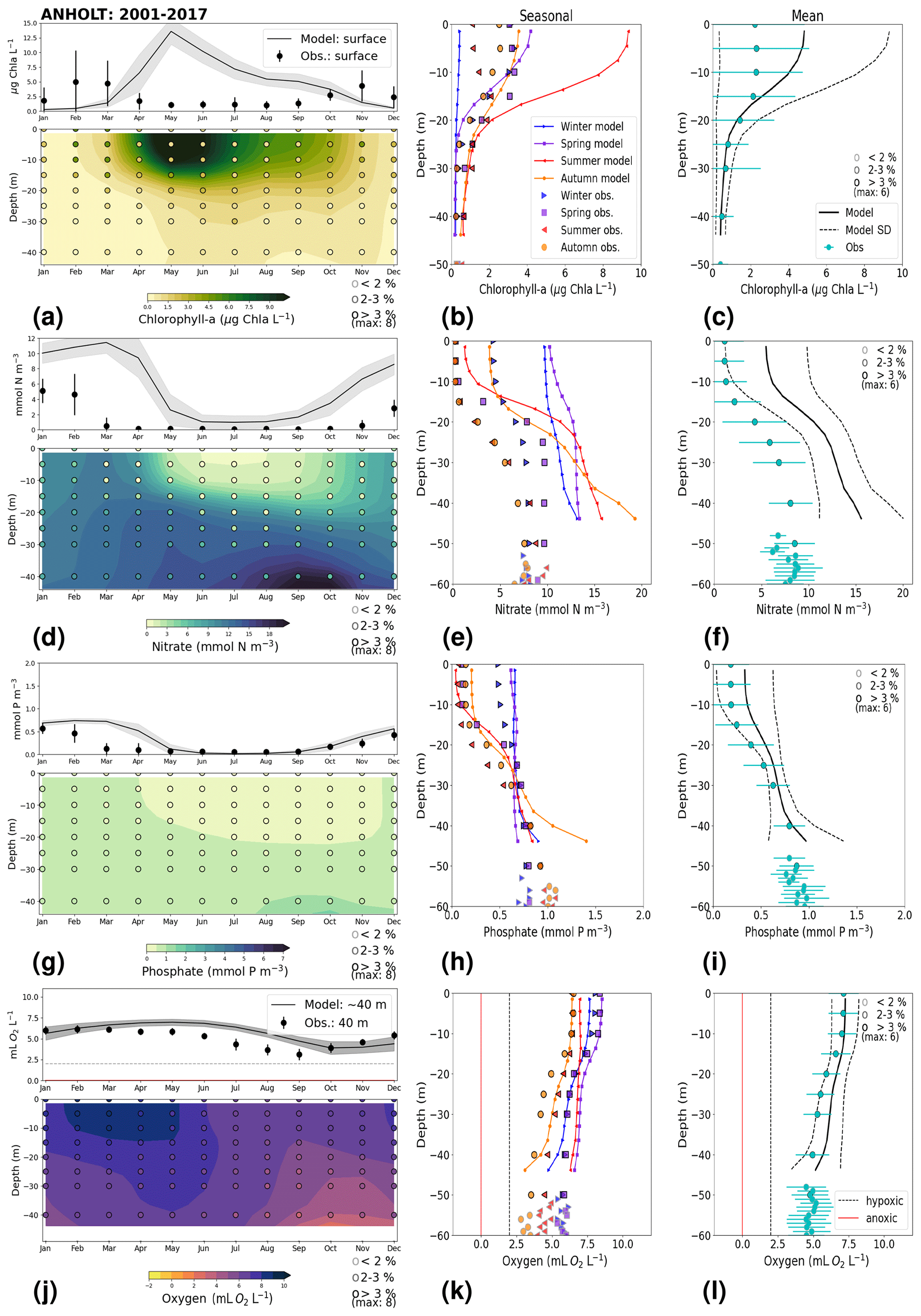
Figure 7Monthly, seasonal and period averages of the main biogeochemical variables at ANHOLT for 2001–2017. Variables are (a–c) chlorophyll a, (d–f) nitrate, (g–i) phosphate and (j–l) dissolved oxygen for both the model and observations. Monthly averages (a, d, g, j) are shown over the entire water column (colours), and a close-up is presented for surface waters for all variables except for dissolved oxygen, for which a close-up of near-bottom waters is shown instead. Here, near-bottom water is considered to be the depth within the last model depth that has the most observations. The standard deviation in time for each averaged monthly value is shown for the model as a grey shaded area and as bars for the observations. The standard deviation of the period means (c, f, i, l) is also displayed for both the model (dashed lines) and observations (cyan crosses). The observational coverage in all plots is shown as open symbols with shades of grey, as indicated in the legend.
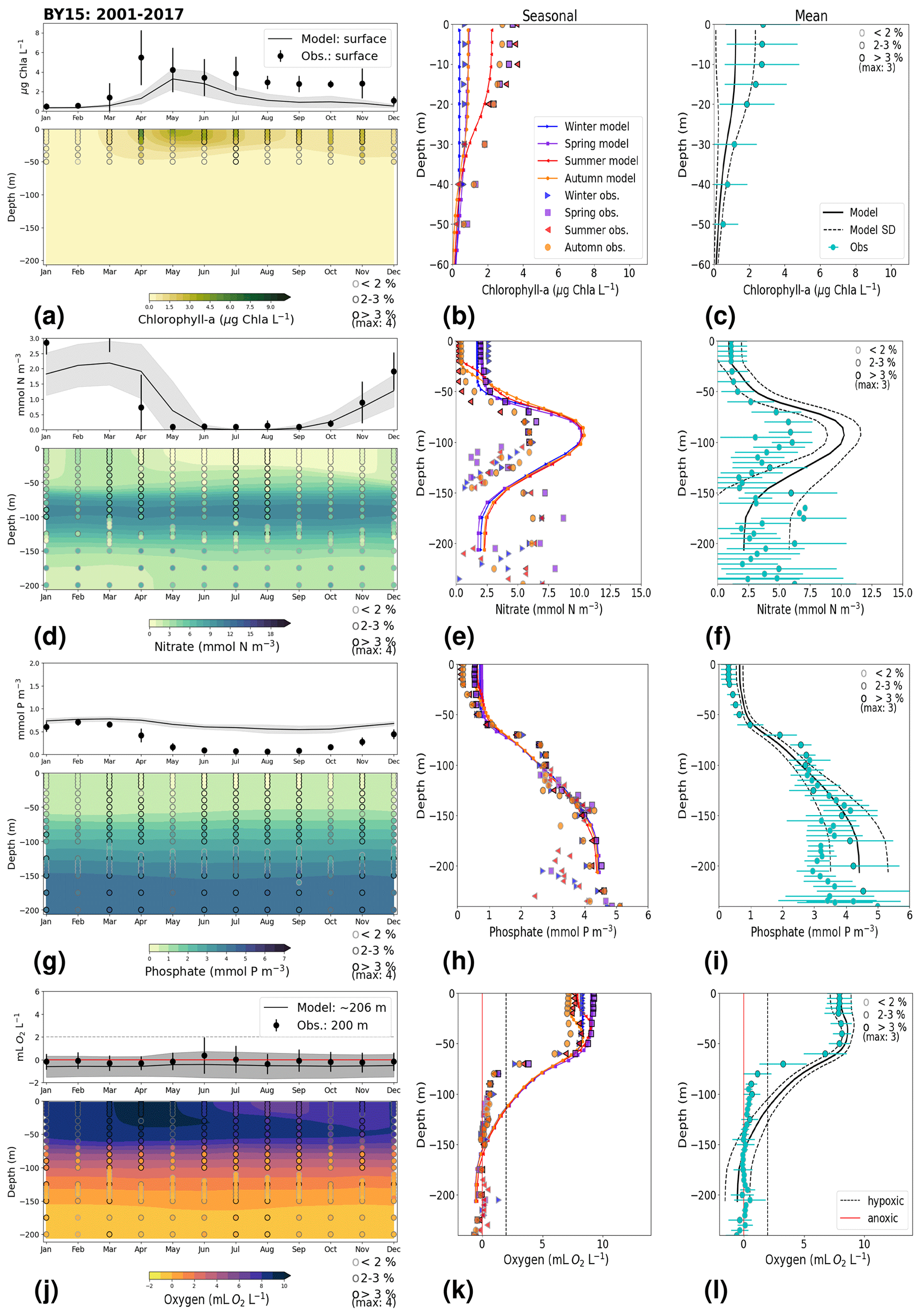
3.1.2 BY15: Baltic Proper
At BY15, the temperature and surface salinity are well captured by the model (Fig. 8a, b). Importantly, the timing of the inflows from the Skagerrak–Kattegat transition zone to the Baltic Proper (reflected by the observed temperature and salinity peaks in bottom waters) are in good agreement with observations and previous findings (e.g. Gustafsson, 1997; Omstedt et al., 2004; Lass and Matthäus, 1996; Feistel et al., 2008; Hordoir et al., 2015). Modelled surface and bottom nitrate as well as bottom phosphate follow the observations at BY15 well, both with respect to the long-term trends (Fig. 8c, d; Table 2) and the interannual variability range (Fig. 9c, d). However, phosphate in surface waters is consistently overestimated by the model (Fig. 8c), especially in late-spring and summer (with a positive bias of ∼ 0.5 mmol P m−3; Fig. 9g), and it does not get fully consumed each year due to an imbalance in the surface N-to-P ratios.
The model results suggest a small but significant increasing trend in chlorophyll-a concentrations from 1975 to 1996 (Fig. 8e, Table 2). After this, the trend slowly decreases until the end of the period in both the model and observations. This period trend is visible at other stations in the Baltic Proper with similar or better observational coverage (i.e. BY1, BY5 and BY31), although with p values generally higher than 0.05. The increasing trend in chlorophyll a is in good agreement with a long-term increase in primary production for ∼ 1980 to 2004 found by Daewel and Schrum (2013). However, the model does not show equally high maxima in chlorophyll a compared with those observed around 1995–2000 at BY15 (Fig. 8e). Such high chlorophyll-a values (> 15 µg Chl a L−1) are rarely captured by in situ measurements, but they are not uncommon when derived from satellite sensors which, for example, have shown summer patches with concentrations higher than 60 µg Chl a L−1 near the entrance of the Gulf of Finland and the southern Baltic Proper (Reinart and Kutser, 2006; Dabuleviciene et al., 2020). This suggests that the model does not capture high growth rates of phytoplankton bloom in the Baltic Proper, which may cause imbalances in the model N-to-P ratios. Here, due to such uncertainties, chlorophyll-a observations are used more as an indication of how well the general patterns are reproduced by the model, rather than as a quantitative parameter. In bottom waters, oxygen follows the salinity, where oxygen maxima coincide with salinity peaks. This indicates that the timing and intensity of the oxygenation events at BY15 are well reproduced by the model (Fig. 8f). These inflows from the Kattegat bring oxygenated waters with high nitrate but low phosphate concentrations, which are also captured by the model (Fig. 8c, d).
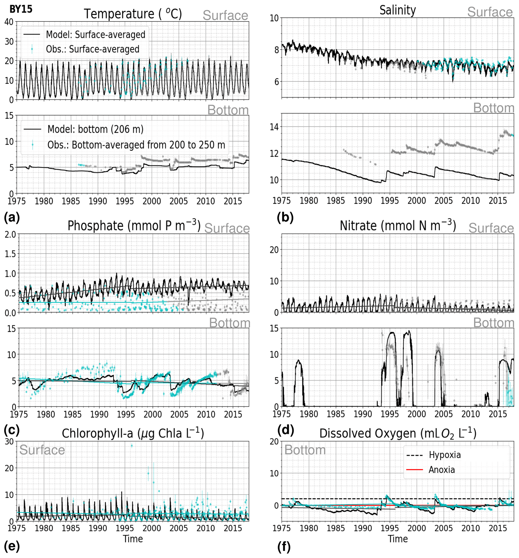
Figure 8Time series of temperature, salinity and main biogeochemical parameters at BY15. Detailed description is as in Fig. 6.
The monthly, seasonal and period averages of chlorophyll a and nitrate are well represented by the model at BY15 (Fig. 9a–c, d–f). Profiles of the modelled oxygen above the halocline and in bottom waters averaged on monthly, seasonal and period timescales are also in good agreement with observations. However, the model shows an increasing bias in oxygen and nitrate with depth and time around the halocline (∼ 75 m). Applying river forcing, which includes daily instead of monthly runoff, significantly improved the surface salinity results in the Baltic Sea when compared with the results in Hordoir et al. (2019), but it increased the existing negative bias in the intermediate and deep waters of the Baltic Proper. As a result of this negative bias, stratification in the Baltic Proper is weaker in the model than in observations, with less-saline, more-nitrate-enriched and more-oxygenated intermediate waters (Fig. 9d–f, j–l). The positive oxygen bias (of max 3 mL O2 L−1) in intermediate waters is only found at the deeper stations (e.g. BY10, BY15 and BY20). This bias also decreases with depth and is linked to the salinity bias that brings less-saline and more-oxygenated inflows to the Baltic Proper. The more-oxygenated intermediate waters lead to less denitrification and, therefore, more nitrate, explaining the overestimation of nitrate at these depths (∼ 75–150 m).
3.2 Model skill at selected stations
The model skill for phosphate, nitrate, chlorophyll a and oxygen for the period from 2001 to 2017 and the seasonal model skill are analysed at 14 stations distributed in the Skagerrak–Kattegat transition zone, the Bornholm Basin, the western Gotland Basin, the eastern Gotland Basin and the northern Baltic Proper. All of these stations show good model skill for both the period and the seasons when evaluated for temperature and salinity (Fig. 10a, b); therefore, the CF and 1−r values for the biogeochemical variables are mainly representative of the SCOBI model performance.
The phosphate model skill for the entire period at all evaluated stations has low enough CF and 1−r values to be placed within the outer quarter circle in the model skill figure, with most stations falling within the inner circle (Fig. 10c, black markers). More specifically, all stations located in the Baltic Proper as well as most stations in the Skagerrak–Kattegat transition zone show good phosphate model skill, except SLÄGGÖ, Å13, FLADEN and W LANDSKRONA, which show acceptable model skill. The model skill to reproduce seasonal phosphate is scattered, although with CF values lower than or close to 1 and combined values of CF and 1−r mainly falling within the inner and outer quarter circles. The latter indicates good or acceptable performance, respectively. However, at ANHOLT, FLADEN and SLÄGGÖ, CF and 1−r values for winter and spring fall outside the outer circle (Fig. 10c, blue and purple markers).
Despite the positive bias in nitrate in the Skagerrak–Kattegat transition zone, the model shows acceptable (mainly good) performance for nitrate when evaluated for the entire period at all 14 stations (Fig. 10d, black markers), except at BY29. The seasonal model performance for nitrate is less well reproduced than that for phosphate, but most stations still show acceptable seasonal performance, except at BY29, ANHOLT, Å13, FLADEN and SLÄGGÖ for all seasons; Å15 for winter and spring; and BY20 for winter (Fig. 10d, colour markers). For the stations in the Skagerrak–Kattegat transition zone, this is due to the time delay in the phytoplankton bloom, which shifts the seasonal cycle in the model (e.g. Figs. 7a–f, B1a–f) and contributes to the positive nitrate bias. This bias is confined above the mixed-layer depth, therefore mainly affecting most of the water column at shallow stations. Because the model considers an averaged depth within a grid cell, the maximum depth of the model and the observations differ. The difference is considerable at shallow stations (with depths less than 100 m), namely, SLÄGGÖ, Å13, ANHOLT, FLADEN and W LANDSKRONA. Observations deeper than the maximum model depth are, thus, not considered in this evaluation; this affects our results, as nitrate below the mixed-layer depth is better captured by the model in this region. At BY29, the poor model skill comes from the bias below the mixed-layer depth linked to the ocean model salinity bias in the Baltic Proper. At this station, the maximum model depth is ∼ 160 m, while observations go as deep as 180 m (not shown). Unlike all the other deeper stations in the Baltic Sea (e.g. Fig. B2), the nitrate bias at BY29 also decreases with depth but remains positive below ∼ 70 m, resulting in a high CF and 1−r. BY29 has not been used for model validation in previous studies; however, BY15 and a nearby station (BY31) in the RCO-SCOBI model show similar results for a different time period (1969–1998), where nitrate CF values are high (>1) below 100 m (Eilola et al., 2009). This suggests that SCOBI still struggles to reproduce nitrate concentrations in the intermediate waters of the Baltic Proper.
In the Baltic Proper, good model skill for chlorophyll a is found at six stations (i.e. BY4, BSCIII-10, HANÖBUKTEN, BY10, BY15 and BY20), which also show good or acceptable model skill for both nitrate and phosphate. The model skill to reproduce oxygen concentrations both seasonally and for the entire period is good at all 14 stations. This is also the case at the other stations in the Baltic Sea (Table B1 in Appendix B). To a lesser extent, the other biogeochemical variables also show good or acceptable model skill at many of these other stations, especially for phosphorus. The main inference of this analysis is that model results at stations in the Skagerrak–Kattegat transition zone and Baltic Proper are good, except at stations where the model delay in the phytoplankton bloom or the positive nitrate bias due to a small oxygen positive bias affects most of the water column. Despite such specificities of the NEMO–SCOBI model, the analysis for individual stations is in good agreement with previous station results in other models (e.g. Eilola et al., 2009; Daewel and Schrum, 2013; Maar et al., 2011).
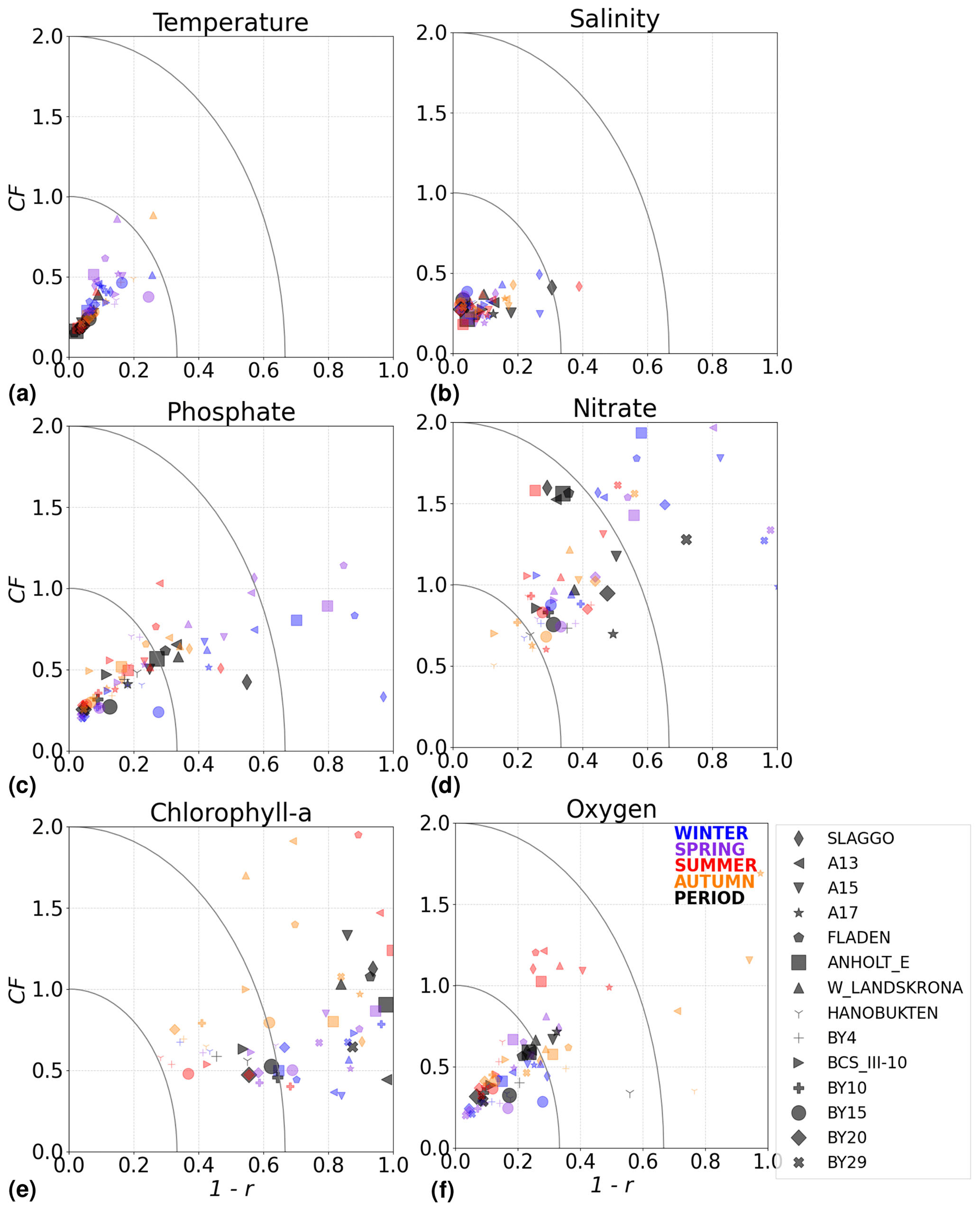
Figure 10Model skill for the period from 2001 to 2017 shown as a combination of the Pearson correlation bias (1−r) and cost function bias (CF) for selected stations in the Skagerrak–Kattegat area and the Baltic Sea. Biases are shown for the whole period (black) and for each season (colours) for (a) temperature, (b) salinity, (c) phosphate, (d) nitrate, (e) chlorophyll a and (f) oxygen in the water column. Winter months are from December to February, spring months are from March to April, summer months are from May to August and autumn months are from September to November. Markers within the inner quarter circle indicate good model skill, markers inside the outer circle indicate that the model skill is acceptable and markers outside the quarter circles indicate large biases. The ANHOLT and BY15 stations are highlighted with larger markers.
3.3 Model skill at regional scales
Physical and biogeochemical processes do not follow political or clearly defined borders. However, the applied HELCOM–OSPAR assessment areas likely represent major features of the regional ecosystems, as they are defined according to geography, bathymetry and stratification, notably that of OSPAR which follows stratification patterns described in van Leeuwen et al. (2015) and Capuzzo et al. (2013, 2015). We use these areas to evaluate the temporal and spatial model skill and, with this, identify dominant model regional features at a subbasin scale or finer scales where possible. In general, this analysis shows that the biogeochemical parameter that is best captured by the model is oxygen, followed by phosphate, nitrate and then chlorophyll a. However, the combined CF and 1−r values, especially when evaluated per HELCOM–OSPAR assessment area, show large scatter for all biogeochemical parameters (Fig. 11). Notably, phosphate and nitrate show variable model skill, which indicates a strong region-specific model response to the ocean dynamics and the applied physical and biogeochemical forcing. Below surface waters (Fig. B5), the model skill for phosphate and nitrate show higher 1−r and CF values in most areas, suggesting that the scattered results are also partly linked to the distribution and frequency of observations. Indeed, observations are not homogeneously distributed in space and time (e.g. Figs. 12, 13) and are seriously lacking in several areas, especially in the North Sea where phosphate and nitrate observations are mainly confined to the surface waters (Fig. 5) and only densely measured in near-coastal regions (van Leeuwen et al., 2023).
More specifically, oxygen shows good or acceptable model skill when evaluated for the entire domain and all subbasins (Fig. 11d, diamonds). Phosphate and nitrate show good and acceptable model skill, respectively, when evaluated for the entire domain, but the skill level differs for each subbasin (Fig. 11a and b, diamonds). Phosphate shows good and acceptable model skill in the Baltic Sea and the Skagerrak–Kattegat transition zone, respectively, in good agreement with previous North Sea–Baltic Sea 3D ocean models (Daewel and Schrum, 2013; Maar et al., 2011), but poor skill in the North Sea. The latter is linked to a mainly negative bias of winter phosphate in most surface waters of the North Sea (Fig. 12a). Nonetheless, 10 out of the 19 evaluated areas in the North Sea (areas 1, 5, 6, 8, 9, 11, 13, 23, 25 and 26; Fig. 11a, circles) show good or acceptable model skill for phosphate. Phosphate biases through all seasons are also found in surface waters of the Skagerrak–Kattegat transition zone and the Baltic Proper (Fig. 12a). However, both of these regions have been more frequently measured than the North Sea, contributing to better and more robust results of the combined CF and 1−r evaluation. The only areas that plot outside the outer circle in the Baltic Sea and the Skagerrak–Kattegat transition zone are the Gulf of Riga and the Bay of Mecklenburg, respectively (areas 33 and 39). Our results give better CF results for phosphorus and oxygen in the Baltic Sea (Fig. 11, green diamonds) than those reported from a model ensemble using ERGOM, BALTSEM and RCO-SCOBI (Eilola et al., 2011a), but they give worse model skill for nitrate.
On the other hand, nitrate is better captured than phosphate when evaluated for the entire North Sea, but it shows poor skill in the Skagerrak–Kattegat transition zone and the Baltic Sea (Fig. 11b, diamonds). In the Skagerrak–Kattegat transition zone, the nitrate bias is linked to the model underestimation of phytoplankton growth and the delay in its monthly maximum. Nevertheless, both the Baltic Sea and the Skagerrak–Kattegat transition zone have a 1−r value and a CF value close to 0.66 and 1, respectively, indicating similarities between the model and observations with respect to both variability and averages. In the Skagerrak–Kattegat transition zone, most HELCOM–OSPAR assessment areas show acceptable nitrate model skill (Fig. 11b, circles), except in the Sound and Kiel Bay (areas 31 and 32, which plot outside the outer circle). Both of these areas have narrow straits and complex land features that likely prevent the model from capturing their full local dynamics. In the Baltic Sea, four HELCOM assessment areas (areas 35, 37, 38 and 43 in Fig. 1) show acceptable model skill, which includes areas where intermediate waters showed a positive nitrate bias at individual stations (e.g. BY5, BY38 and BY15 in the Bornholm Basin, the western Gotland Basin and the eastern Gotland Basin; areas 35, 37, 38 in Fig. 11b). This suggests that the model overestimation of nitrate in intermediate waters and that in surface waters shown at stations in the Skagerrak–Kattegat transition zone mainly affect the model skill in the Arkona Basin (area 34), which plots outside the outer circle when evaluated at all depths (Fig 11b) and in surface and intermediate waters (Fig. B5b, c). However, model biases in surface waters for nitrate in the Arkona Basin are mainly found in winter and spring and along the southern coast (northern Germany and Poland; Fig. B6b).
Furthermore, in the northern Baltic Proper, the Gdańsk Basin, the Gulf of Riga, the Gulf of Finland, the Åland Sea, the Quark and Bothnian Bay, the model skill for nitrate is less good. In the northern Baltic Proper, the surface model bias is mainly confined along the coast and near the entrance of the Gulf of Finland, resulting in acceptable model skill for surface waters in this area (Figs. B6b, 11b). In the Bothnian Sea, intermediate waters give acceptable model skill for nitrate (Fig. B5c), but poor skill is found with respect to surface waters (Fig. B5b). All other northern basins in the Baltic Sea show poor nitrate skill in intermediate waters. This suggests that the nitrate bias in the model for the northern basins of the Baltic Sea is not linked to that of the Skagerrak–Kattegat transition zone and the Baltic Proper; rather, it is linked to specific regional inputs and local dynamics. The applied atmospheric nitrate input in the Baltic Sea, especially for years before 1995, may be overestimated here. In this case, nitrate concentrations in areas where phytoplankton are limited by phosphate could slowly increase with time due to the fact that nitrate is not fully consumed each year. A small overestimation of nitrate in such areas (such as in the Gulf of Bothnia) would also lead to nitrate accumulation in these areas and explain the positive bias. Our results compare well to the CF results for surface waters in Maar et al. (2011), where their highest values are also found near coastal areas in the Baltic Proper and the Bothnian Sea for both phosphate and nitrate. Note that, in their study, observations for the Gdańsk Basin, the Gulf of Riga, the Gulf of Finland and Bothnian Bay are missing. In fact, except for the northern Baltic Proper and the Gdańsk Basin, the Gulf of Riga, the Gulf of Finland, the Åland Sea, the Quark and Bothnian Bay are the most poorly measured of the Baltic Sea, which prevents robust statistical evaluations in these areas.
On a finer regional North Sea scale, the model skill for nitrate is acceptable in several shallow areas in the southern and eastern parts of the North Sea (areas 1, 7, 9, 11, 22 and 26), the Dogger Bank (area 5) and the Norwegian Trench (area 6). While the northern North Sea (area 25) plots far outside the outer circle, the eastern North Sea (area 24) plots near the outside circle (with a CF close to 1.25 and a 1−r close to 0.6), suggesting that areas less affected by the northern open boundary and direct riverine nutrient input (i. e. southern offshore areas) are best represented by the model. In addition, the northern North Sea (area 25 in Fig. 1) is the largest assessment area of the North Sea and has the poorest data coverage regarding phosphate and nitrate (Figs. 12, 13). This makes it difficult to analyse specific model flows in this area. Note, however, that the nutrient bias in the northern North Sea surface waters is generally small in all seasons (Fig. B6). Nonetheless, our biogeochemical results are comparable to those of Daewel and Schrum (2013), which is in overall good agreement with observations in the North Sea but with biases along the southern coast of the North Sea. This region is characterized by strong tidal currents (Van der Molen, 2002) and is heavily impacted by runoff and nutrient input that results in a high spatio-temporal variability. This remains a challenge for most models to recreate, as also highlighted in a recent model ensemble study (van Leeuwen et al., 2023).
The best model skill for chlorophyll a is in the North Sea (with a CF lower than 1 and a 1−r slightly higher than 0.66), within which five of the evaluated HELCOM–OSPAR assessment areas show acceptable model skill (areas 1, 2, 9, 12 and 18; Fig. 11c, circles). These regions, located in the southern North Sea, are well-mixed coastal areas (van Leeuwen et al., 2015) where phytoplankton are mainly N limited in spring (both shown in observations and model results; Fig. 14). This suggests that the model is able to reproduce chlorophyll a, even in regions where important nutrient discrepancies between the model and observations exist, as long as the limiting nutrient for phytoplankton growth in the model corresponds to that in observations. Small model imbalances between nitrate and phosphate can greatly affect chlorophyll-a production, especially when the stoichiometry is fixed to the Redfield ratio (Fransner et al., 2018; Neumann et al., 2022). This could lead to large bias in chlorophyll a through all seasons in many areas of the model domain (Fig. B6c in Appendix B). Oxygen measurements for the five areas where the model skill for chlorophyll a is best (areas 1, 2, 9, 12 and 18; Fig. 11c, circles) are lacking, but all evaluated areas in the North Sea (i.e. with more than 100 observations; Fig. 5) show good model skill for oxygen below the surface, except the northern North Sea (area 25; Fig. 11, circles). The northern North Sea is directly influenced by the open boundary conditions in the model. Applying simplified physical dynamics and biogeochemistry in the open boundaries likely limits our model results in this area.
The model skill analysis at a regional scale shows that the model response varies widely, giving an overall acceptable model skill for oxygen, nutrients and chlorophyll a that is comparable to other model studies. Regional discrepancies between the model and observations exist that are difficult to explain due to complex physical and biogeochemical interactions, but the following three potential causes affecting different regions could be identified: the local nutrient input (via rivers or atmosphere), the applied open boundaries and a missing process in the phytoplankton growth that delays the peak of the bloom in the model (as further discussed in Sect. 3.6). The spatio-temporal lack of observations greatly hinders a more detailed understanding of the system. Thus, larger regional-scale processes are the main focus of the next section.
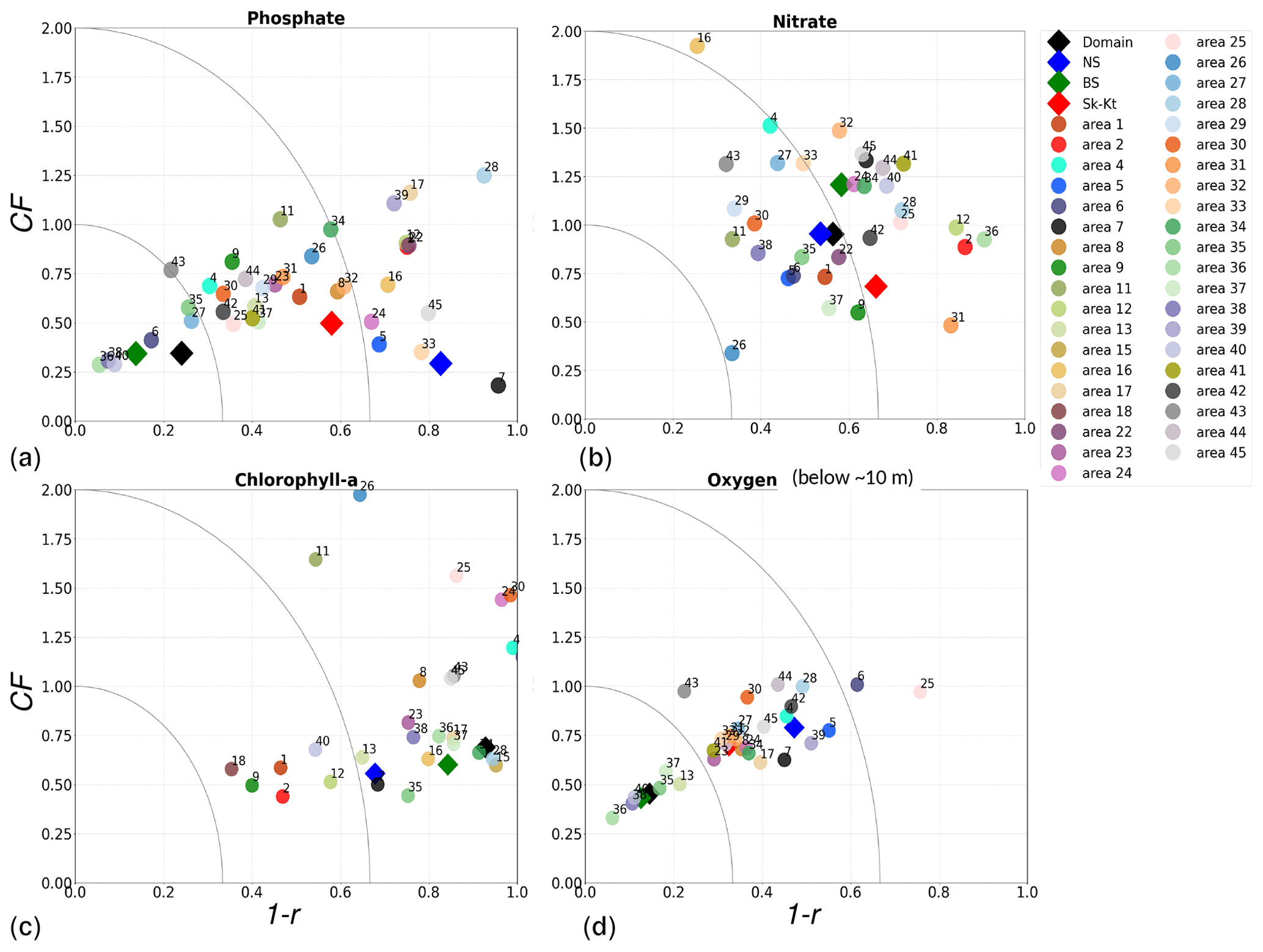
Figure 11Model performance over the period from 2001 to 2017 shown as a combination of the Pearson correlation bias (as 1−r) and the cost function bias (CF) for the Baltic Sea (BS), North Sea (NS) and Skagerrak–Kattegat (Sk-Kt) transition zone (diamonds) as well as the areas in Fig. 1 (circles). Numbers in the legend correspond to evaluated areas; note that additional areas are not evaluated for oxygen due to lack of observations (see Sect. 2.2.3 and Fig. 5). Chlorophyll a is evaluated for the top ∼ 10 m, and oxygen is evaluated below the surface waters.
3.4 The North Sea–Baltic Sea system
The coastal zone along France, Belgium, the Netherlands, Germany, and Denmark is characterized by nitrate accumulation, which reflects phosphate limitation of primary productivity in this region (Figs. 12, 13, 14, B3, B4). To a lesser extent, phosphate also accumulates close to the shoreline along the southeastern North Sea, likely because productivity rates there are not high enough to fully consume the massive nutrient input by rivers (as seen both in observations and model results). Productivity in this region is likely limited by light (Holt et al., 2012). The nitrogen accumulation pattern is promoted by the reduction in phosphorus loads in the early 1990s (e.g. Burson et al., 2016; Ly et al., 2014) and is well captured by the model (Figs. 12, 13, 14). The main river sources in this area are the Rhine, Elbe, Scheldt and Meuse plumes, where elevated nitrogen is discharged each year (Fig. 3). In the northern North Sea, the pattern is inversed: almost full consumption of nitrate takes place in spring/summer, whereas phosphate is preserved throughout the year. Phosphorus sources are mainly point sources, from input via rivers and from advected water masses coming from the North Atlantic, which are enriched in nutrients due to mixing and internal wave generation along the shelf break (Gröger et al., 2013; Mathis et al., 2019; Huthnance et al., 2022).
High riverine nutrient inputs and shallow water depths promote high chlorophyll-a concentrations along the coasts (Holt et al., 2012). The elevated chlorophyll-a concentrations along the eastern UK coast have been shown to be likely related to frequent upwelling events under a predominant westerly wind regime (Winther and Johannessen, 2006). Towards the open ocean, chlorophyll-a concentrations tend to decrease. In particular, autumn and winter mixing in the central North Sea (van Leeuwen et al., 2015) distributes chlorophyll a deep along the water column. The Norwegian Coastal Current is characterized by mesoscale meanders and eddies (Ikeda et al., 1989). Mesoscale eddies are also produced along the opposing currents of the northward flowing Norwegian Coastal Current and the southward flowing water masses entering the North Sea at the western slope of the Norwegian Trench (Winther and Johannessen, 2006). Hence, nutrients from deep waters can be mixed upwards, especially in winter and spring. When nutrients enter the stratified waters of the Norwegian Coastal Current, chlorophyll-a concentrations increase in this region. During autumn, the chlorophyll-a concentrations decrease due to increased vertical mixing caused by strong winds (Sündermann and Pohlmann, 2011). All of these chlorophyll-a main features can be clearly seen in the chlorophyll-a maps for spring, summer and autumn, in both the model results and observations (Figs. 12, 13), indicating that the model is able to reproduce these North Sea characteristics. In addition, the spatial distribution of both nutrients and the N-to-P ratios are well captured by the model, which show important persistent gradients in the entire domain (Figs. 12, 13, 14, B3, B4). In particular, strong nutrient gradients are observed in the Skagerrak–Kattegat transition zone, which is in good agreement with previous findings for the Skagerrak (Danielssen et al., 1997). However, a consistent positive bias in nitrate occurs in the coastal southeastern North Sea, in the Skagerrak–Kattegat transition zone (as described before at individual stations in this region), near the Szczecin Lagoon (Poland), and in the gulfs of Gdańsk, Riga, Finland and Bothnia (Fig. B6in Appendix B). In the Skagerrak, the observations show an overall nitrogen limitation except during the spring months (Fig. 14b). In this area, the model remains phosphorus limited in all seasons due to the positive nitrogen bias (Fig. 14a).
In the more stratified Baltic Sea, nutrients and chlorophyll-a concentrations are spatially more homogeneous. Unlike in the North Sea, the high chlorophyll-a concentrations in the Baltic Sea are confined to the coasts (Figs. 12, 13) due to the limited occurrence of mesoscale turbulence and, in turn, poor mixing in the open Baltic Sea (Feistel et al., 2008). Both of these physical features are well represented in the model (Hordoir et al., 2019). The open Baltic Sea is fuelled by the direct nutrient input along the coasts and by nutrients accumulated in seawater and sediments during winter. The nutrient inventory decreases in surface waters due to consumption by phytoplankton and export of sinking organic matter during the growth season, which spans from late winter/early spring to late-summer/autumn (Fig. 13), varying according to region and between the open and coastal ocean. In the Baltic Proper, primary productivity is limited by nitrate (as clearly seen in Fig. 14) linked to high removal rates of nitrogen via denitrification and high release rates of inorganic phosphorus from the sediments (Eilola et al., 2009). This favours cyanobacteria blooms under elevated temperatures and reduced vertical mixing during (late-)summer (Janssen et al., 2004). In the model, the cyanobacteria bloom starts in summer but only becomes widespread in autumn (Fig. B7 in Appendix B). This could be linked to a model overestimation of light attenuation in the open ocean (Fig. B8 in Appendix B) limiting cyanobacteria growth in the summer months. In addition, explicitly considering the life cycle of cyanobacteria would significantly improve the timing of the growth of cyanobacteria (Hense and Burchard, 2010; Hieronymus et al., 2021). The cyanobacteria response likely affects the entire phytoplankton growth season in the model, which is currently generally underestimated in the open Baltic Sea (Fig. B6c) and starts 1 month later compared with observations (Fig. 9a). Hence, nutrient depletion is also perturbed in the model results. In the Bothnian Sea and Bothnian Bay, the seasonal cycle of nitrate is not well captured, which is common in models using a fixed Redfield ratio (Fransner et al., 2018; Neumann et al., 2022).
In the southeastern coastal North Sea and in the Skagerrak–Kattegat transition zone, the model delay with respect to the phytoplankton bloom is about 3 months. According to observations, chlorophyll-a concentrations in both of these areas peak in late winter (around February), whereas the maximum occurs in May in the model. Here, the model late-winter/early-spring primary productivity is not limited by nitrogen, phosphate or silicate. In addition, the maximum growth rates were adjusted to favour diatoms under lower temperatures and high nutrient concentrations (Sect. A1, Eq. A7 and Table A1 in Appendix A). However, this is not sufficient to capture the correct timing of the phytoplankton bloom in the Skagerrak–Kattegat transition zone. This suggests that an additional limiting factor affects both the southern coastal North Sea and the Skagerrak–Kattegat transition zone. The model sensitivity of total phytoplankton growth rates to temperature and light attenuation is shown in Fig. A1 in Appendix A, where nutrients, detritus and zooplankton concentrations are kept constant at typical model values for February in the Kattegat. The model does not allow for high phytoplankton growth rates (or a high chlorophyll-a concentration) at low temperatures and low light attenuation (high secchi depths). Indeed, the modelled temperature at ANHOLT is low (2.5 °C), the secchi depth high (6.8 m) and the chlorophyll-a concentrations low (∼ 1 µg Chl a L−1). Because the model temperature for February in surface waters (when averaged from 2001 to 2017) is very close to that shown by the observations (2.8 °C), we attribute the phytoplankton bloom delay mainly to an overly low sensitivity of phytoplankton growth to light in this region (Fig. A1, Appendix A). The delay in the model causes interannual nutrient imbalances that can be transported, for example, along the Jutland coastal waters into the Skagerrak, where this imbalance persists, affecting the seasonal nutrient concentrations in the Kattegat (e.g. excess of phosphorus in summer; Figs. 7, B1).
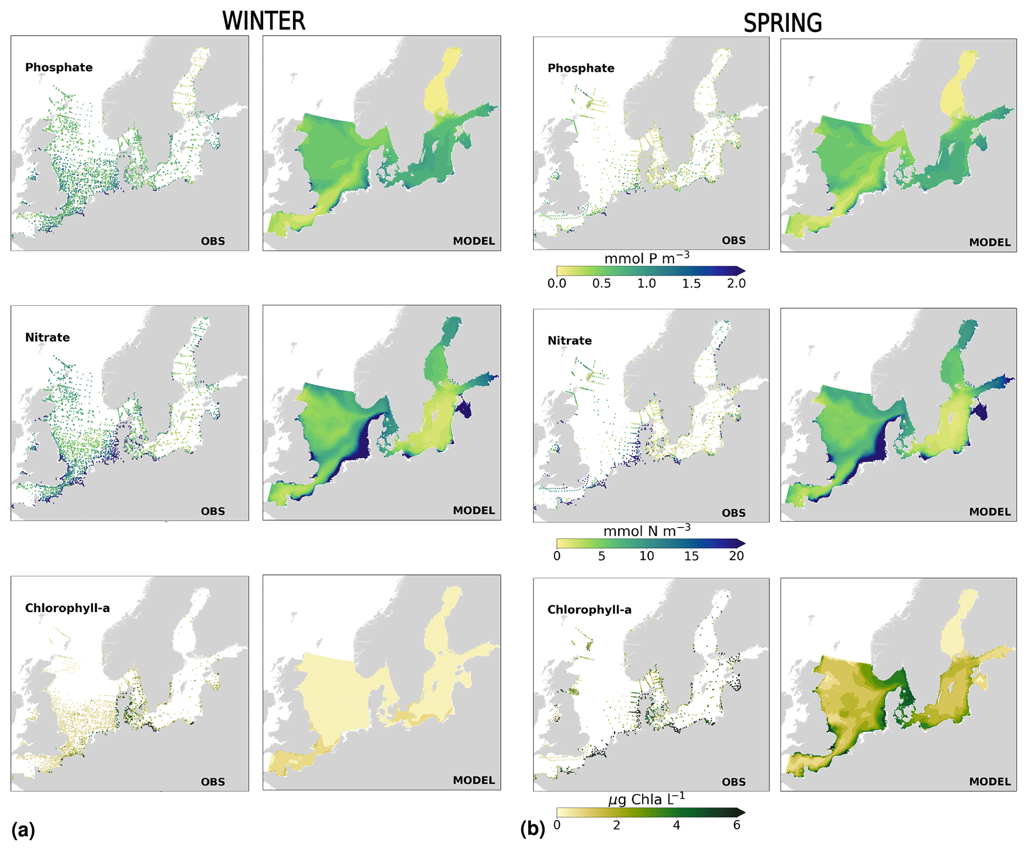
Figure 12Spatial distribution of (a) winter and (b) spring for observations (left panels) and model results (right panels) for phosphate, nitrate and chlorophyll a averaged over the period from 2001 to 2017.
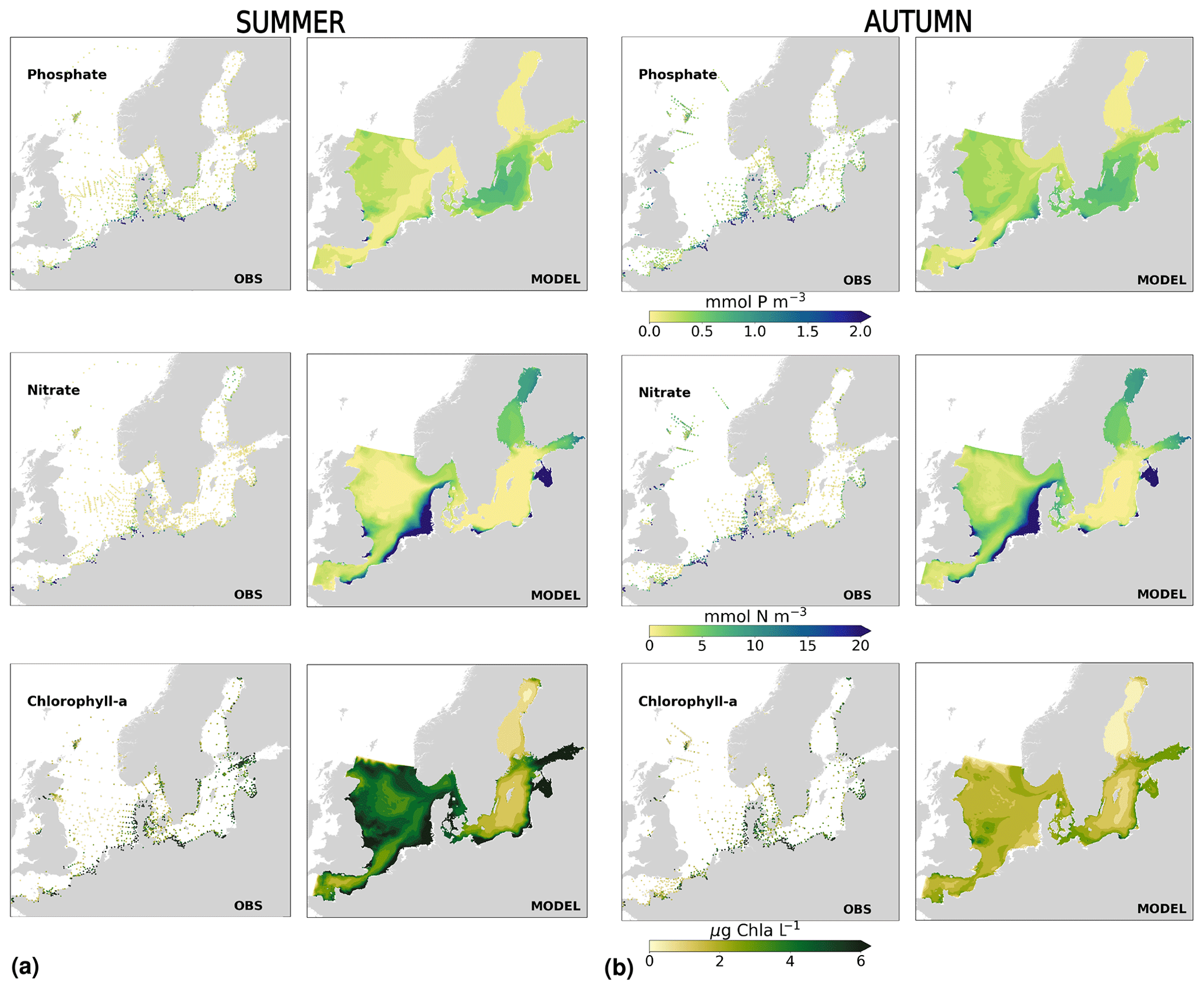
Figure 13Spatial distribution of (a) summer and (b) autumn for observations (left panels) and model results (right panels) for phosphate, nitrate and chlorophyll a averaged over the period from 2001 to 2017.
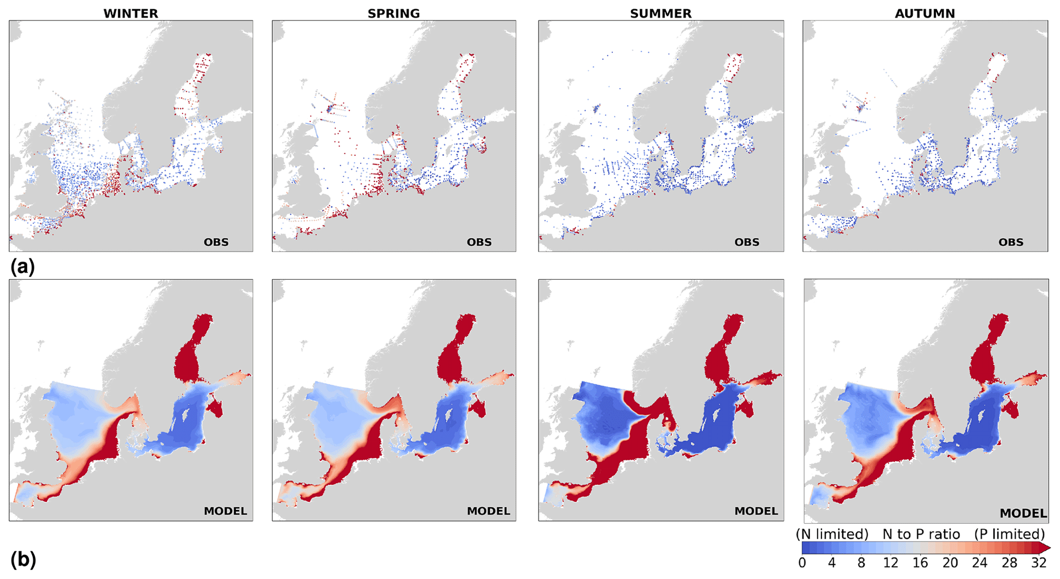
Figure 14Seasonal nitrogen to phosphate ratios for the period from 2001 to 2017 for (a) observations and (b) model results.
3.5 Relevance of the study
Previous ocean models coupled to SCOBI (e.g. Eilola et al., 2009; Almroth-Rosell et al., 2011) have the open boundary in the Kattegat. The main advantage of this model set-up compared with those models, as well as with the typical model used to support HELCOM assessments (Gustafsson et al., 2012; Savchuk et al., 2012), is that NEMO–SCOBI allows for study of the North Sea and the entire Skagerrak–Kattegat transition zone, as the boundaries have been moved far from the Kattegat area. Covering the entire Swedish coast and the newly covered Skagerrak–Kattegat transition zone is particularly important for Swedish marine managers. The latter is a complex, dynamic area that is difficult to simplify in order to represent correct in-/outflows as boundary conditions (Gustafsson, 1997). This is especially true for long-term modelling, as conditions in this region depend on the modelled processes in the adjacent basins, rather than prescribed boundary conditions. For climate runs, it is, for example, difficult to prescribe boundary conditions at the high resolution needed in order to resolve the influence of processes in the North Sea and Skagerrak. Thus, extending the boundaries far from the Skagerrak–Kattegat transition zone allows for a better representation of its full dynamics.
When compared to other modelling studies, covering either one sea or both seas, our results show differences that are neither better nor worse than previous model results depending on the variable and area (e.g. Eilola et al., 2011a; Maar et al., 2011; Daewel and Schrum, 2013). This has also been demonstrated in a recent ensemble study on eutrophication that includes NEMO–SCOBI results (van Leeuwen et al., 2023), where, for example, chlorophyll-a concentrations were both over- and underestimated by the different models used in the ensemble when compared with satellite and in situ observations in the southern North Sea and the English Channel (areas 7 and 11 in Fig. 1). It is, nonetheless, surprising that, by expanding the model to cover such a different dynamic region and with very little additional tuning, most processes in the North Sea are still well captured.
Here, we have not only validated our model results for individual stations but also for areas officially used in international programmes aiming to reduce eutrophication, such as OSPAR and HELCOM. To our knowledge, this is the first time that model results from one single model have been validated for the combined HELCOM–OSPAR assessment areas. Following the statement of Ducrotoy and Elliott (1997), Mee et al. (2008), and Koho et al. (2021) regarding a need for improved ecosystem models in these areas, we provide a step forward towards better understanding model-area-dependent performance and uncertainties. This also provides added value with respect to contributing to joint OSPAR and HELCOM initiatives, especially to their work on healthy environments. Importantly, a variety of models simulating the biogeochemistry in similar areas should be used together, as they all differ significantly in their biogeochemical complexity and have different performance skill. The use of ensemble mean assessments has been shown to be good or even better than the results from individual models (Eilola et al., 2011a; van Leeuwen et al., 2023). We have shown that the NEMO–SCOBI model can be used to derive relevant indicators for HELCOM and OSPAR initiatives for the North Sea–Baltic Sea system, for which specific, relevant improvements will be applied. Large model biases, especially that of nitrate, are also strongly linked to the applied forcing, which is continuously updated depending on available data and/or down-scaling methods. Thus, the model will be used to produce novel climate and nutrient scenarios similar to those provided by the Climate Change Scenario Service (https://www.smhi.se/en/climate/future-climate/advanced-climate-change-scenario-service/oce/, last access: December 2023), produced by the SMHI, but now with a consistent model domain that covers the entire North Sea–Baltic Sea system.
3.6 Future work and knowledge gaps
Solving the phytoplankton bloom timing in the southeastern coastal North Sea and the Skagerrak–Kattegat transition zone in NEMO–SCOBI is a priority, as it would significantly improve the model results, especially with respect to nitrate concentrations and the seasonal behaviour of the biogeochemical parameters. Our ecosystem model study suggests that, besides nutrients, the light attenuation in the North Sea is key to determining the specific spatial distribution of phytoplankton communities, in agreement with the findings in Ford et al. (2017) for the North Sea. Seasonal observations that relate to light attenuation coefficient (Kd) (or secchi depths) are less abundant than those for nutrients in the entire domain, especially in the North Sea. However, when comparing NEMO–SCOBI results for secchi depths to winter-averaged observations reported in ICES for the North Sea during the period from 2001 to 2017, NEMO–SCOBI tends to underestimate secchi depths (by 1–5 m depending on the location) in the open waters of the North Sea, whereas it overestimates winter secchi depths (by 1–5 m) in a narrow fringe of the southeastern coastal waters (Fig. B8a in Appendix B). We have also compared our results to light attenuation averages for different areas in the North Sea from Capuzzo et al. (2013, 2015) and found that Kd values in NEMO–SCOBI are in very good agreement with those reported in these studies for most areas and seasons, with notably small differences (∼ 2 m) in the open southeastern and northern North Sea for winter and spring. However, better constraining the spatial distribution of Kd, included in the parameterization for phytoplankton growth (Eqs. A1 and A3 in Appendix A), could significantly improve our results. In addition, the current parameterization of the light attenuation in NEMO–SCOBI does not allow for the co-occurrence of high phytoplankton growth rates, low temperatures and high secchi depths, as inferred from winter observations in the Skagerrak–Kattegat transition zone (Figs. 12a, A1). This suggests that the parameterization of light attenuation in NEMO–SCOBI is well adapted for open waters, but additional tuning is required for specific shallow areas, such as the Skagerrak–Kattegat transition zone and the southern coast of the North Sea.
Moreover, substance-specific attenuation coefficients from measurements are not well constrained. Maar et al. (2011) made a comparison between a model run considering a constant background value for Kd versus one with a salinity-dependent Kd. The latter gave a better correlation between model results and observations, improving the timing of their model spring bloom. Their approach remains an approximation of realistic Kd levels and calls for a dedicated study on light limitation for phytoplankton growth. For our model, one important factor affecting the light attenuation coefficient is the organic matter present in seawater. Therefore, future work will also consist of better capturing the detritus in the SCOBI model. However, detritus in the North Sea–Baltic Sea system is poorly observed and, therefore, poorly constrained. Seasonal comparisons between the model detritus and organic phosphorus and nitrogen observations in surface waters (obtained by subtracting the inorganic nitrogen/phosphorus from the total nitrogen/phosphorus in the ICES data set) suggest that the model underestimates detritus in coastal areas near point sources, especially in the southeastern North Sea, and slightly overestimates it during winter in the central North Sea (not shown). One factor affecting detritus is the fraction of the organic matter coming from rivers that is actually bioavailable and not directly retained in coastal waters. Here, we have assumed a constant bioavailable fraction for the riverine organic nitrogen and phosphorus (of 0.3 and 0.75, respectively) in the entire domain based on previous studies for the coast in the Baltic Sea (e.g. Nausch and Nausch, 2007; Eilola et al., 2009; Asmala et al., 2017; Edman et al., 2018). Thus, the input of organic matter from rivers, especially nitrogen, could be improved by better accounting for river-specific organic matter retention in coastal waters. However, this fraction is highly uncertain, especially in coastal waters in the North Sea, and would require additional sensitivity tests. Importantly, both the ICG-EMO and the Baltic Sea data sets, on which our correction factors for nutrient loads are based, come with large uncertainties (Savchuk et al., 2008; Lenhart et al., 2010; Gustafsson et al., 2012). From a sensitivity test in which the river loads were changed (not shown), the largest effect on nutrient concentrations in surface waters, affecting both coastal and the open ocean, was found in the southern North Sea and in the Arkona Basin. Additional effects were restricted to highly river-influenced coastal areas.
Water column and benthic denitrification (Fig. 15) are two important processes that can remove nitrogen from the system. These are well studied in the Baltic Sea; however, they are still poorly constrained on a seasonal basin-wide scale, and long observational time series are also lacking. In the central Baltic Sea (east of Gotland), estimates of water column denitrification in autumn/summer for the years 2008 and 2010 are variable, but they can be as high as 21 (Dalsgaard et al., 2013; Hietanen et al., 2012). Water column denitrification rates averaged from 2001 to 2017 for summer and autumn in the hindcast run are comparable to but slightly lower than these estimates (Fig. 15a). The total nitrogen removal from water column denitrification in the Baltic Proper with persistent large hypoxic areas has been estimated to be 132–547 kt N yr−1 (Dalsgaard et al., 2013). In the model, the yearly rates in the Baltic Proper vary between 40 and 129 kt N yr−1 during the period from 2001 to 2017, with an average of 65 kt N yr−1 for the entire period. An improved mixing representation below the halocline in the Baltic Proper would further improve the model oxygen concentrations in the intermediate waters of the aforementioned region. This would, in turn, lead to higher denitrification rates and decreased nitrogen concentrations there. Consequently, nitrogen transport to the adjacent basins (such as the gulfs of Riga, Finland and Bothnia) would likely decrease; therefore, the nitrate positive bias in such basins would be reduced. One way of improving the vertical mixing in NEMO would be to increase the vertical resolution of the model, as discussed in Hordoir et al. (2019).
Benthic denitrification has been estimated in the Gulf of Bothnia (0–0.94 ; Stockenberg and Johnstone, 1997; Bonaglia et al., 2017), in the Gulf of Finland (0.1–0.65 ; Tuominen et al., 1998; Hietanen and Kuparinen, 2008), in the northern Baltic Proper (0.014–0.3 ; Tuominen et al., 1998) and in the southern Baltic Proper (0.012–0.69 ; Deutsch et al., 2010). In these basins, the benthic denitrification rates in the model are in good agreement with previous estimates, although at the lower end of the ranges (Fig. 15b). The seasonal variations in benthic denitrification in the Baltic Sea are poorly observed, but they have been found to follow a marked seasonal cycle, with low rates in early spring increasing towards late summer to late autumn and decreasing towards late winter (Hietanen and Kuparinen, 2008). While this seasonal variation in benthic denitrification is not well captured by the model, the yearly rates are in good agreement with previous estimates. The nitrogen removal by benthic denitrification in the entire Baltic Sea has been calculated to be between 426 and 652 kt N yr−1 (Deutsch et al., 2010). In the model, the benthic removal rate of nitrogen in the Baltic Sea for the from period 2001 to 2017 varies from 484 to 627 kt N yr−1, with a period average of 553 kt N yr−1. Improving the seasonal cycle of benthic denitrification in the model would likely improve the seasonal variability in the nitrogen in basins with high denitrification rates.
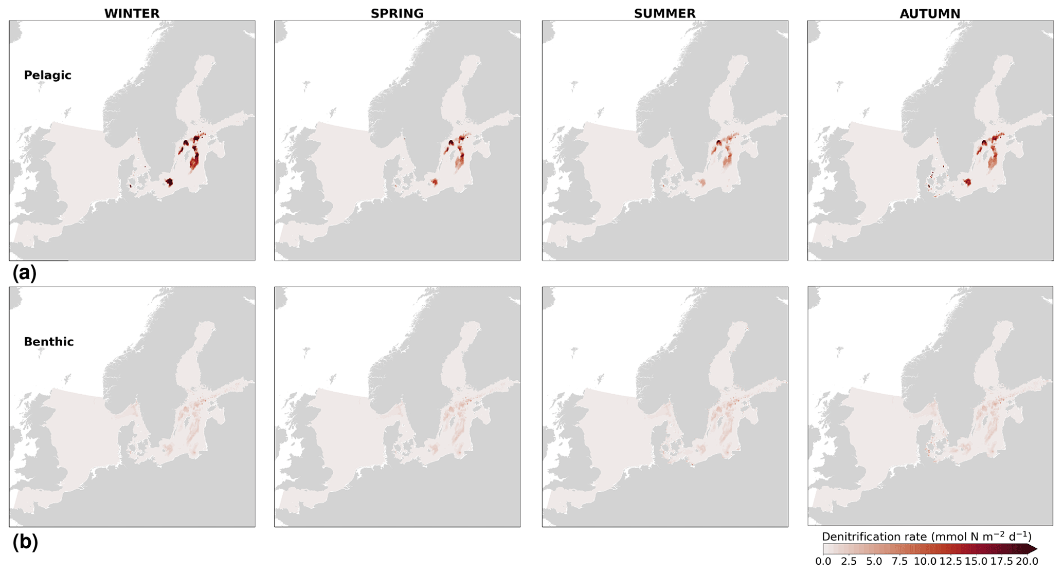
Figure 15Model spatial distribution of seasonal averages of pelagic and benthic denitrification for the period from 2001 to 2017.
Here, we have presented and evaluated NEMO–SCOBI: a new coupled physical–biogeochemical model configuration for the Baltic and North seas. In conclusion, the model simulates biogeochemical variables well, reflects the physical and hydrodynamic processes, reproduces long-term trends, and responds reasonably to anthropogenic nutrient sources along the coastal zone. This makes the model particularly suitable for application in future multi-stressor studies, such as testing combined climate and nutrient scenarios (e.g. Wåhlström et al., 2020). It is, therefore, ready to be used to produce climate projection, such as those in the SMHI Climate Scenario Service. Compared with other Baltic Sea models that have to prescribe climatological boundary values based on a limited number of observations in the Kattegat area (e.g. Eilola et al., 2009; Neumann et al., 2002), NEMO–SCOBI avoids many problems associated with a lateral boundary in the area of the Kattegat and Skagerrak. This is of fundamental importance for the salt and oxygen inventory of the Baltic Sea, as it controls the North Sea–Baltic Sea mass exchange. It was demonstrated that the model simulates this exchange in a physically consistent way with good skill for the oxygen dynamics in the Baltic Sea. NEMO–SCOBI also reveals a realistic seasonal cycle and interannual variability in most of the assessed variables as well as model skill that can fully compete with existing models for the North Sea and the Baltic Sea. Thus, it can be used in further scientific applications, such as for a detailed analysis of long-term nutrient exchanges between basins and climate effects on eutrophication and oxygenation. It should be noted that robust statistical evaluations for long-term trends are particularly difficult to obtain in the northern North Sea, the Gulf of Riga, the Gulf of Finland, the Åland Sea, the Quark and Bothnian Bay due to the great lack of observations in these areas. Including the entire North Sea–Baltic Sea system in one single model (as opposed to previous model versions coupled to SCOBI) allows for better identification of regions with similar biogeochemical behaviour, avoiding limitation to one of the seas, as well as to study different processes occurring in the Skagerrak–Kattegat transition zone. NEMO–SCOBI can also keep contributing to European initiatives on de-eutrophication, water quality advice, and support on nutrient reduction loads of both the North Sea and the Baltic Sea. However, additional care must be taken when evaluating regional seasonal cycles, especially for chlorophyll a and nitrate. NEMO–SCOBI is, to our knowledge, the third physical–biogeochemical model covering the area of the Baltic and the North seas (Daewel and Schrum, 2013; Maar et al., 2011). Future model intercomparison studies of these three model systems have the potential to give valuable scientific insights into model performance and process understanding; thus, NEMO–SCOBI is an important addition to the model ensemble of this region.
A1 Phytoplankton growth in NEMO–SCOBI
Here, we only describe the phytoplankton growth as implemented in the current version and relevant related variables. Involved constant values are listed in Table A1. For a full overview and mass balance equations, the reader is referred to Eilola et al. (2009). The parameterization for phytoplankton growth (GROWTH; Eq. A1) is defined as follows:
All three phytoplankton groups share the same oxygen dependency to prevent anabolism under anoxic conditions (OXLIM; Eq. A2) and light limitation (LTLIM; Eq. A3). These are defined as follows:
Here, the photosynthetic available radiation (IPAR; Eq. A4) decreases exponentially with depth (z), and the optimum irradiation for photosynthesis (IOPT, in W m−2; Eq. A5) is described as follows:
The solar radiation (I0, in W m−2) that reaches the water surface is calculated at every time step within NEMO-Nordic, and IPAR was set to account for light absorption due to biological fluxes. The vertical light attenuation coefficient (Kd) is affected by a constant background light attenuation (Kdw) and by the concentrations of phytoplankton, zooplankton, yellow substances and detritus as follows:
where αphy, αzoo and αDETN are the light attenuation coefficients per unit of chlorophyll a, zooplankton and detritus, respectively, and λys is a regionally prescribed vertical attenuation coefficient for yellow substances.
The three phytoplankton groups have the same fixed mortality rate (5 % of the phytoplankton concentrations per day). They differ from each other with respect to their maximum growth (GMAX; Eqs. A7–A9), which is temperature dependent; their nutrient limitation of the growth (NUTLIM; Eqs. A10–A12); and their sinking rates. Hence, they depend on both the physical and chemical conditions of the water. The group PHY1 has the characteristics of “diatoms” which, besides using nitrogen and phosphorus, use silica to build up their shells. They can grow rapidly under cold conditions and at higher nutrient concentrations, having an advantage over flagellates under turbulent conditions. The group PHY2 represents “flagellates and others” and benefits from stratified conditions, i.e. when surface temperatures are relatively high and the nutrient concentrations are low above the thermocline. The group PHY3 has the characteristics of “filamentous cyanobacteria”, which grow in warm low-salinity waters; therefore, a salinity threshold of S≤10 is used for cyanobacteria only to grow in the Baltic Sea. As in previous versions of SCOBI, cyanobacteria also have the ability to fix molecular nitrogen (N2) when nitrogen concentrations are low in the water. They have a tendency to remain close to the surface waters, so that they are considered to be neutrally buoyant in the model (i.e. their sinking speed is set to zero). The maximum growth for PHY1, PHY2 and PHY3 (GMAX1, GMAX2 and GMAX3, respectively) is defined as follows:
Note that the growth sensitivities to temperature (T) for all phytoplankton types have been tuned for NEMO-Nordic based on sensitivity analysis (see Table A1 for the updated constant values). The silica limitation for group PHY1 was implemented following Michaelis–Menten kinetics. The half-saturation constant for the uptake of silica by diatoms has been shown to be extremely variable depending on the species and water conditions (Thamatrakoln and Hildebrand, 2008). Here, we take a rather conservative value (0.1 mmol Si m−3; Table A1), following Paasche (1973) and Pasquer et al. (2005). The nutrient limitation for PHY1, PHY2 and PHY3 (NUTLIM1, NUTLIM2 and NUTLIM3, respectively) in SCOBI is now as follows:
Here, NLIM, PLIM and SiLIM are the nitrogen, phosphate and silica limitation, respectively:
The and “[ ]” are the half-saturation constants and the concentrations of nitrate, ammonium, phosphate and silica, respectively, and Φ is the strength of ammonium inhibition for nitrate uptake. An example of the total GROWTH as a function of Kd and T for typical model values in surface waters of the Kattegat is shown in Fig. A1. At low Kd (high secchi depth) and low T, phytoplankton growth rates can only be small in the model.
Table A1Constants as applied in NEMO–SCOBI for phytoplankton growth. Numbers in bold are updated or new values based on sensitivity analysis, whereas other numbers follow those in Eilola et al. (2009) or Almroth-Rosell et al. (2015). PHY1 stands for diatoms, PHY2 stands for flagellates and others, and PHY3 stands for filamentous cyanobacteria.
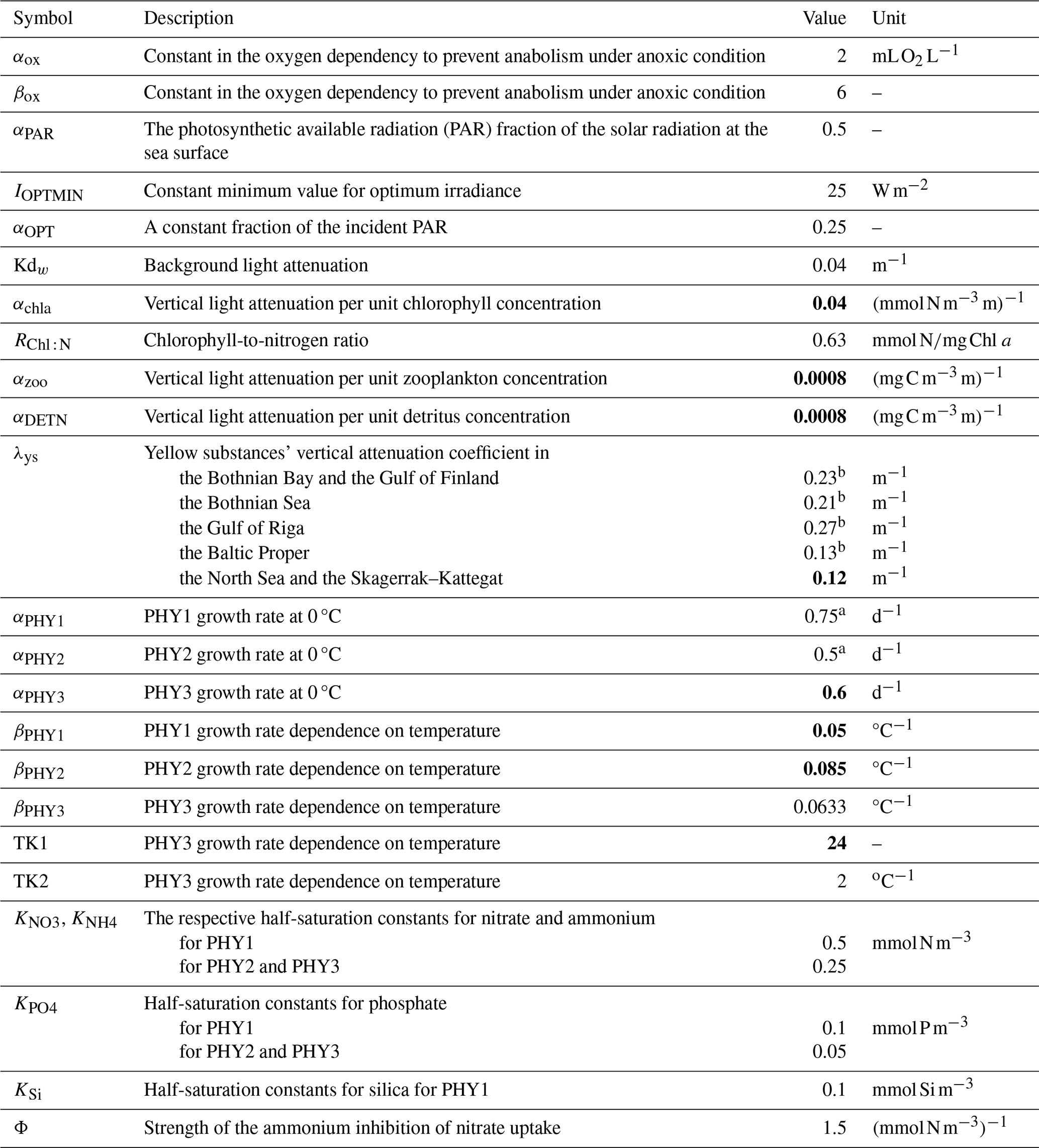
a Applied in the SCOBI version in Almroth-Rosell et al. (2015). b Applied in Eilola et al. (2009).
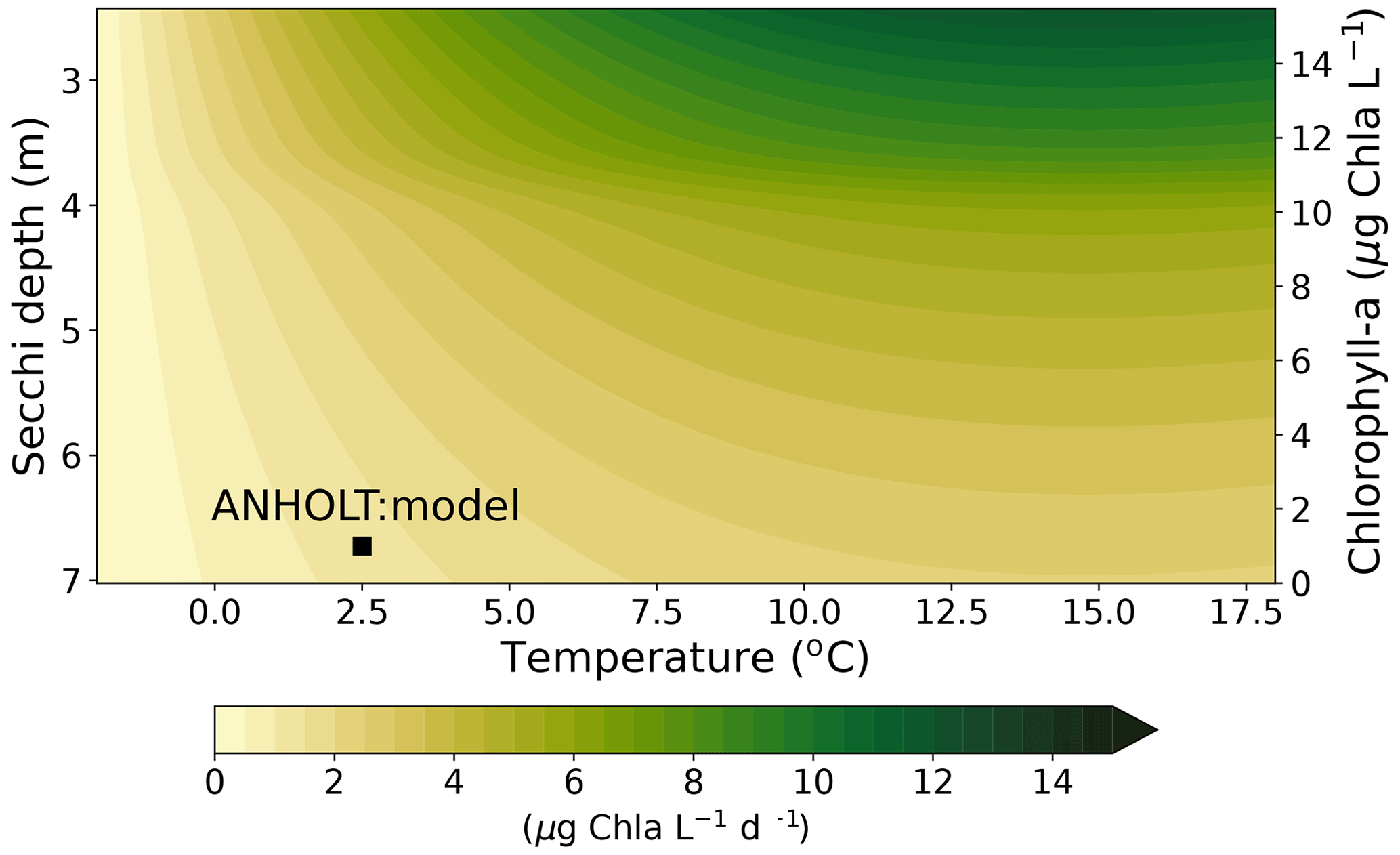
Figure A1Sensitivity of phytoplankton growth to temperature and light attenuation (Kd) given by Eq. (A6) and shown as secchi depth = , which is a general approximation based on Holmes (1970). Except for temperature and concentrations of PHY1, PHY2 and PHY3, all variables in Eqs. (A1) to (A15) are fixed to averaged values for the period from 2001 to 2017 in the Kattegat area at ∼ 4 m depth. The corresponding total chlorophyll-a concentrations () from which Kd was obtained are shown as a reference on the right x axis. The actual model value obtained at ANHOLT for February is highlighted (black square). As a reference, the temperature, the secchi depth and the chlorophyll-a concentrations obtained from observations at ANHOLT are 2.8 °C, 8 m and 5 µg Chl a L−1, respectively.
A2 Benthic fluxes in NEMO–SCOBI
In SCOBI, the sinking organic matter (phytoplankton and detritus) is deposited on the sediments and builds up the corresponding benthic nutrient pools: BSi, BOP and BN. The sinking rate of phytoplankton varies between functional types and follows the velocity sinking function of Penta and Walsh (1995). The sinking velocity of detritus is a function of depth, the detritus pool, and a constant sinking velocity rate set to 2.5 m d−1 in the water column and to 3.5 m d−1 in the bottommost cell to account for aggregation processes, following Neumann et al. (2002). The release of inorganic nutrients from benthic organic material has been modified to better capture the nutrient dynamics for both the Baltic Sea and the North Sea. Similarly to Almroth-Rosell et al. (2015), the total release of phosphorus from remineralized benthic organic material (BOPOUTPO4; Eq. A16) consists of two pathways: the transfer of phosphorus from BOP to the sediment pool of mineral-bound inorganic phosphorus (BOPREMBIP; Eq. A17) and the direct release of phosphate to the overlying water column (BOPREMPO4; Eq. A18). The release of benthic phosphorus is temperature dependent (described by the remineralization rate term λT; Eq. A19), oxygen dependent and now also salinity limited (included in the limitation term δO2S; Eq. A20). In the well-mixed North Sea, BOPREMBIP is generally less important than in the Baltic Sea. Here, BOPREMBIP decreases with increasing salinity (S) and decreasing bottom oxygen concentrations ([O2]bot), which then increases BOPOUTPO4 accordingly, as follows:
Here,
To avoid negative values for BOPREMBIP, BOPREM when λO2S<0.15. The salinity dependency starts at salinities of 20 (dividend in Eq. A20). At even higher salinities, such as those in the North Sea (>30), the transfer of phosphate to BIP does not occur (i.e. BOPREMBIP is approximately 0). However, the bottom-water oxygen concentration ([O2]bot) remains the most important variable controlling the benthic transfer of phosphate to BIP. Under anoxic conditions (i.e. O2≤0), all phosphate from remineralization is directly released to the water column (BOPREMBIP=0.0), independently of the salinity level.
In addition to BOPREMBIP, the BIP pool is increased by the scavenging of PO4 under oxic conditions (PO4SCAVBIP; Eq. A21), whereas it is decreased by the redox-dependent release of inorganic phosphorus from iron-bound-particles (BIPRELPO4; Eq. A22). Both depend on the oxygen concentrations in bottom waters and are parameterized as follows:
The water diffusivity of inorganic phosphorus is given by αpscv, as follows:
The constant values involved in both fluxes (αprel, KBIP, Ko2bot, ΔX, C1sp, C2sp, C3sp and ϕ) are described in Table A2. Note that, from these constants, only ϕ (the sediment porosity) differs from older SCOBI versions. This term was region-specific in previous versions. In NEMO–SCOBI, this term had to be simplified for numerical reasons, but it will be made region dependent at a later stage. In Eq. (A23), Tbot is the bottom-water temperature between 0 and 25 °C. The BIP pool is also affected by the permanent burial of phosphorus (BIPBUR; Eq. A28), the resuspension of inorganic P due to wave and current friction, and sinking of WIP in bottom waters. The resuspension and the sinking of WIP depend on the shear stress, following Eq. (A31).
For the release of nitrogen (in the form of ammonium) from benthic organic matter (BNOUTNH4), the remineralization rate is regulated by the temperature and BN (Eq. A24). The release of silica from benthic organic matter (BSiOUTDSi) is assumed to be directly discharged to the overlying water column in the form of dissolved silica with half the dissolution rate compared with the remineralization rate (Eq. A25):
Other oxygen-dependent benthic processes, such as benthic denitrification and ammonium sequestration on particles, determine how much ammonium enters the water column from the sediments and follow the equations in Eilola et al. (2009). Here, a nitrate limitation term is added to the benthic denitrification of pelagic nitrate (BDENNO3), which removes nitrate from the water column as follows:
Permanent burial of organic matter (BOPBUR, BIPBUR, BNBUR and BSiBUR) depends on a shared but regional constant burial rate (αbur) and the accumulated material within sediments, as follows:
The constant burial rates are prescribed per basin, and respective values are shown in Table A2. The resuspension of benthic organic nutrients due to wave and current friction (S) depends on a prescribed critical shear stress (τcrit), which differs in the Baltic Sea and the North Sea in this work (Table B1), and the mean shear stress (τ), following Almroth-Rosell et al. (2011):
where So is the maximum upward velocity of particles and Ws the sinking velocity. Resuspension occurs when the bottom stress exceeds τcrit; otherwise, the suspended material is (re)deposited in the sediments. Based on sensitivity analysis, a more conservative value for τcrit is used in the Baltic Sea compared with previous SCOBI versions, and a small τcrit was added for the North Sea (Table A2). This is because bottom waters in the North Sea are generally more dynamic than those in the Baltic Sea and, therefore, more sensitive to the resuspension of benthic material (Almroth-Rosell et al., 2011; Thompson et al., 2011).
Table A2Constants as applied in NEMO–SCOBI for benthic processes. Numbers in bold are updated values.
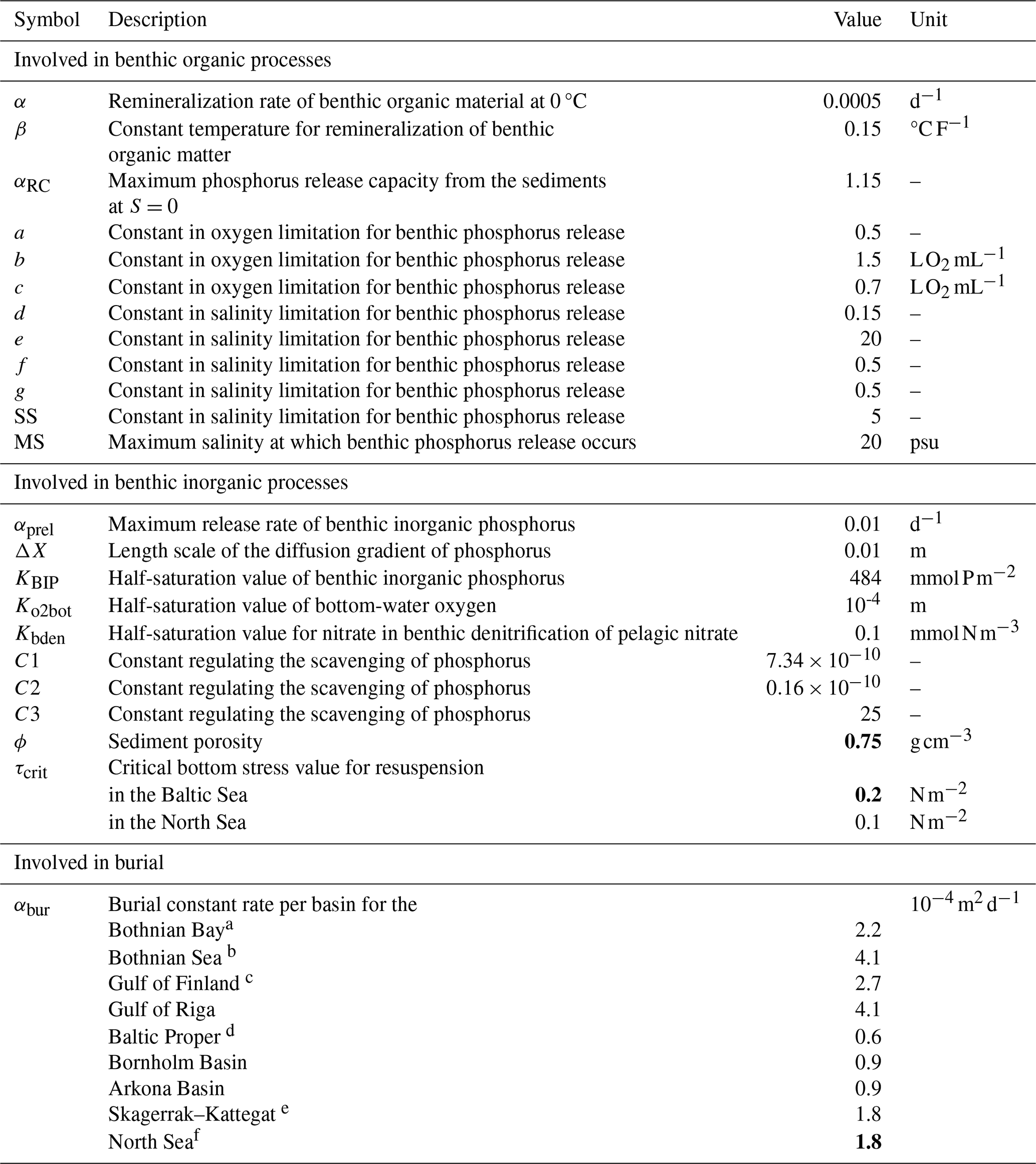
a Includes the Quark. b Includes the western Åland Sea. c Includes the eastern Åland Sea (i.e. Archipelago Sea). d Includes the Gdańsk, western Gotland and northern Baltic Proper basins. e Includes the Bay of Mecklenburg, Kiel Bay, the Sound and the Coastal NOR 3. f Includes all areas in the North Sea.
The following additional results are presented in this section and complement those shown in the main text, mainly as further examples of model performance:
-
Table B1 presents the model skill of phosphate, nitrate, chlorophyll a and oxygen at additional stations (Sect. 3.2).
-
Figs. B1 and B2 outline the monthly, seasonal and the yearly averages over the period from 2001 to 2017 at Å17 in the Skagerrak and BY5 in the Bornholm Basin, respectively. The biogeochemistry above 60 m at Å17 and ANHOLT is as described in the main text (Sect. 3.1). However, below such depth, at the deep stations of the Skagerrak–Kattegat transition zone (namely, Å15 and Å17), the model is in good agreement with observations and shows little monthly, seasonal or annual variability (e.g. Fig. B1). Note that nitrate is only underestimated by the model below 60 m at Å17. The biogeochemistry at BY5 is similar to that at BY15, as described in the main text (Sect. 3.1), and only small differences can be observed at BY5, principally due to the fact that BY5 is shallower than BY15. For example, at BY5, no positive oxygen bias in intermediate waters (below ∼ 75 m) is displayed by the model, as salinity is still well captured at this station and at these depths.
-
Figs. B3 and B4 show time series of water column nitrate and phosphate at three of the stations in the southern North Sea that include the largest number of observations. Model results are compared to observations and show a general good agreement with respect to both magnitude and seasonality. However, high nitrate concentrations linger in the model, especially at Walcheren due to a frequent lack of summer depletion. Because the number of observations remains lower than those from the SHARK stations (especially at EastCoastNS), these stations have not been included in the statistical analysis (e.g. regression analysis and model skill per station).
-
Fig. B5 presents the spatio-temporal model performance at a fine regional scale for phosphate and nitrate for surface, intermediate and deep waters.
-
Fig. B6 gives the seasonal spatial distribution of differences between the model results and observations for three main biochemical parameters in surface waters (namely, nitrate, phosphate and chlorophyll a). The figure shows that the difference between the model and observation varies by season and variable, especially for chlorophyll a. The smallest difference in phosphate is found in the Gulf of Bothnia for all seasons, in the northern North Sea in winter and in the southern North Sea in summer. For nitrate, the smallest differences between model and observations are mainly in the central North Sea and the Baltic Proper in all seasons.
-
Fig. B7 shows the seasonal spatial distribution of the three included phytoplankton species in surface waters. It is clear that flagellates dominate in summer in the model, while cyanobacteria are mainly restricted in the Baltic Proper during autumn, when diatoms and flagellates decrease and nitrate concentrations are low.
-
Fig. B8 presents the seasonal spatial distribution of observed secchi depths. When compared with model results, it shows that there is a general overestimation of the modelled secchi depths in the open ocean and the Skagerrak–Kattegat transition zone but that the light penetration is best captured in the Baltic Sea during summer.
Table B1List of the total number of observations (nobs), the 1 – correlation coefficient (1−r) and the cost function (CF) for the period from 2001 to 2017 at 12 stations in the Baltic Sea that are not shown in Fig. 10 for 4 main biogeochemical parameters. The 1−r and the CF are evaluated for the entire period (p), for winter (w), for spring (sp), for summer (s) and for autumn (a). A “−” indicates that no observations were available for the corresponding evaluated time period. Numbers in black indicate good or acceptable model skill, where good model skill is highlighted in bold (i.e. when both 1−r and CF are smaller than 0.35 and 1, respectively). Numbers in typewriter or italic font indicate poor model skill (i.e. when both 1−r and CF are larger than 0.7 and 2, respectively) “close to outer circle” and “far from the outer circle”, respectively. When nobs is less than 500, the variable at that stations is not considered in this analysis.
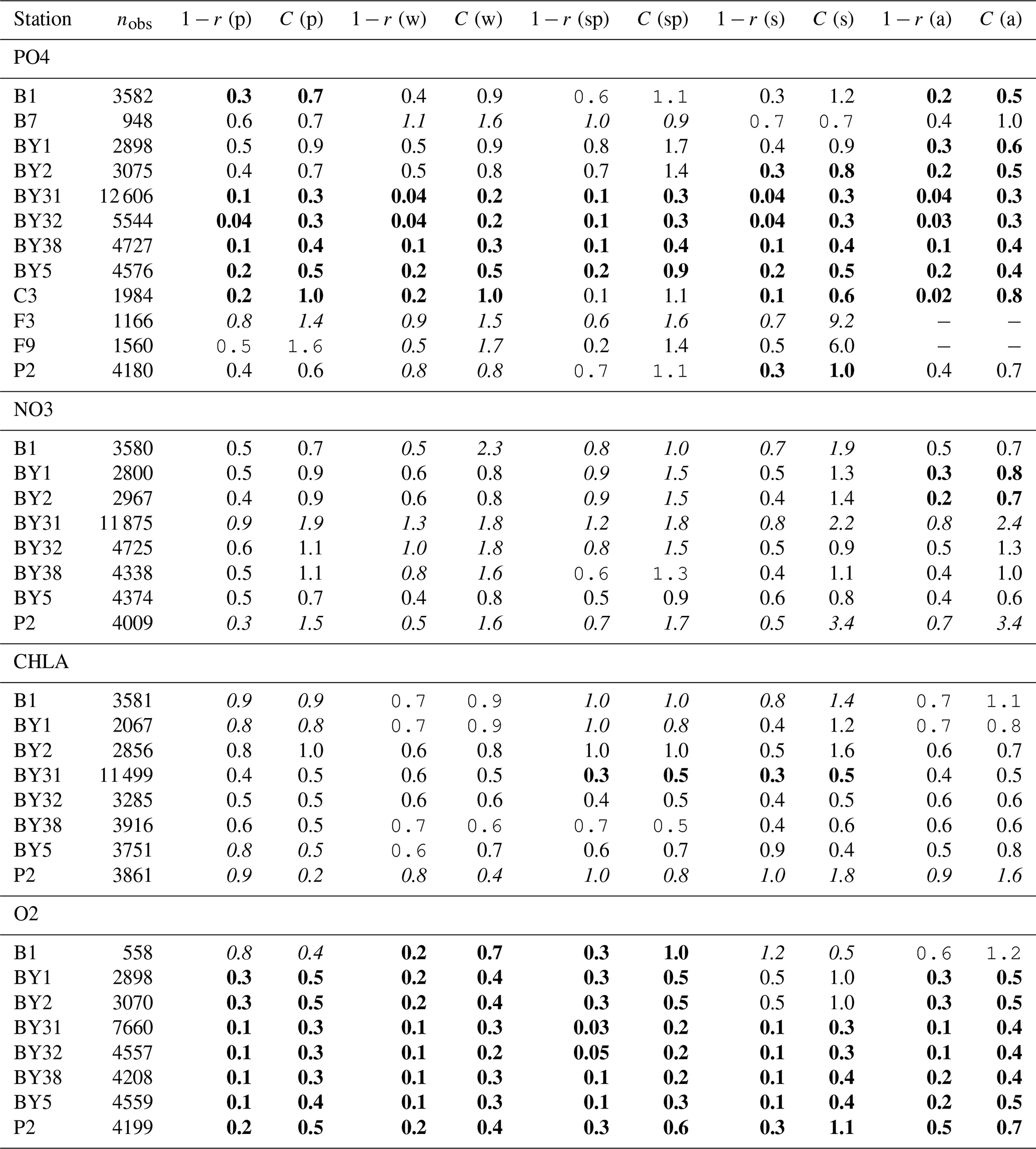
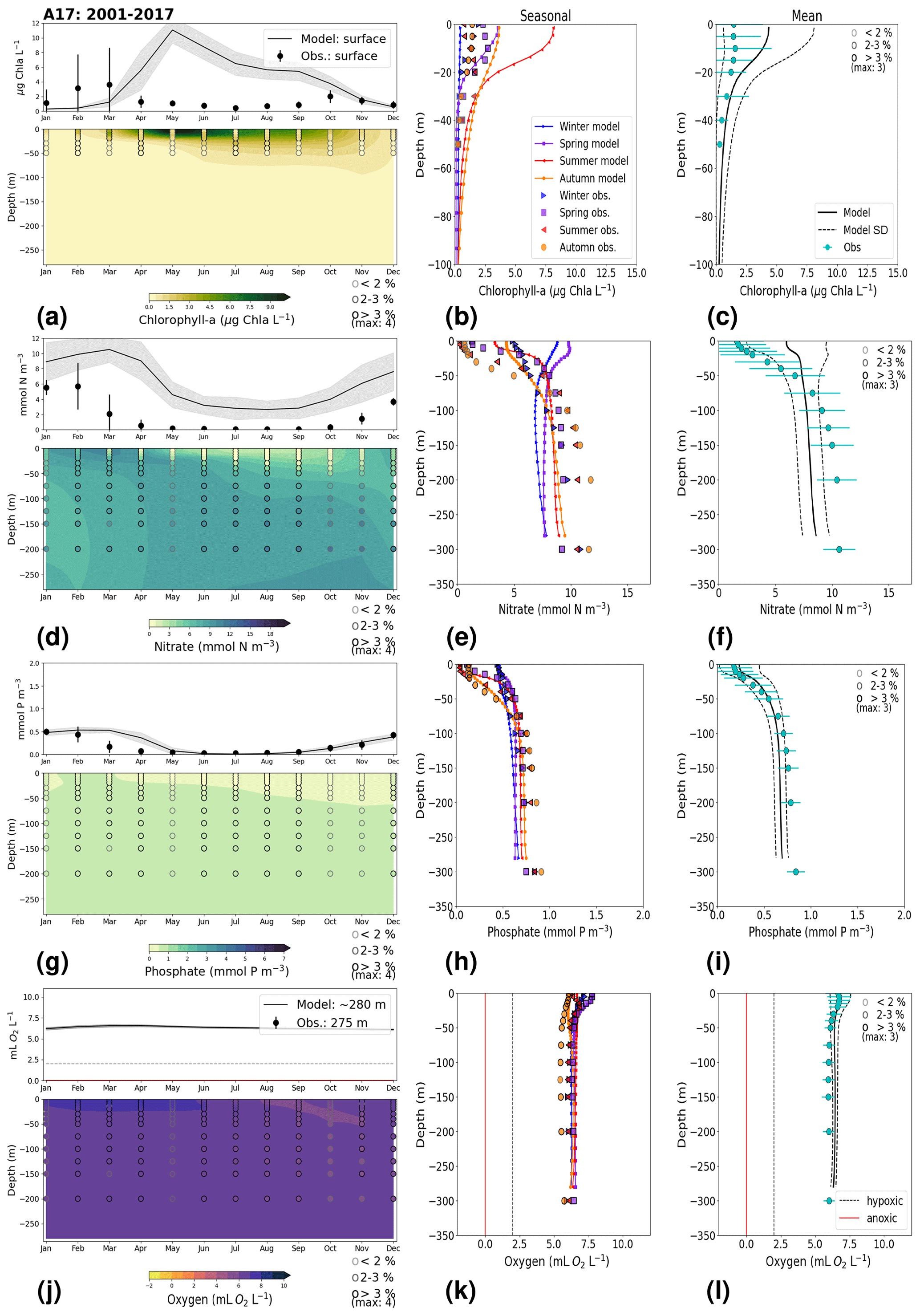
Figure B1Monthly, seasonal and period averages of the main biogeochemical variables at Å17 for 2001–2017. Variables are (a–c) chlorophyll a, (d–f) nitrate, (g–i) phosphate and (j–l) dissolved oxygen for both the model and observations. Monthly averages (a, d, g, j) are shown over the entire water column (colours), and a close-up is presented for surface waters for all variables except for dissolved oxygen, for which a close-up of near-bottom waters is shown instead. Here, near-bottom water is considered to be the depth within the last model depth that has the most observations. The standard deviation in time for each averaged monthly value is shown for the model as a grey shaded area and as bars for the observations. The standard deviation of the period means (c, f, i, l) is also display for both the model (dashed lines) and observations (cyan crosses). The observational coverage in all plots is shown as open symbols with shades of grey, as indicated in the legend.
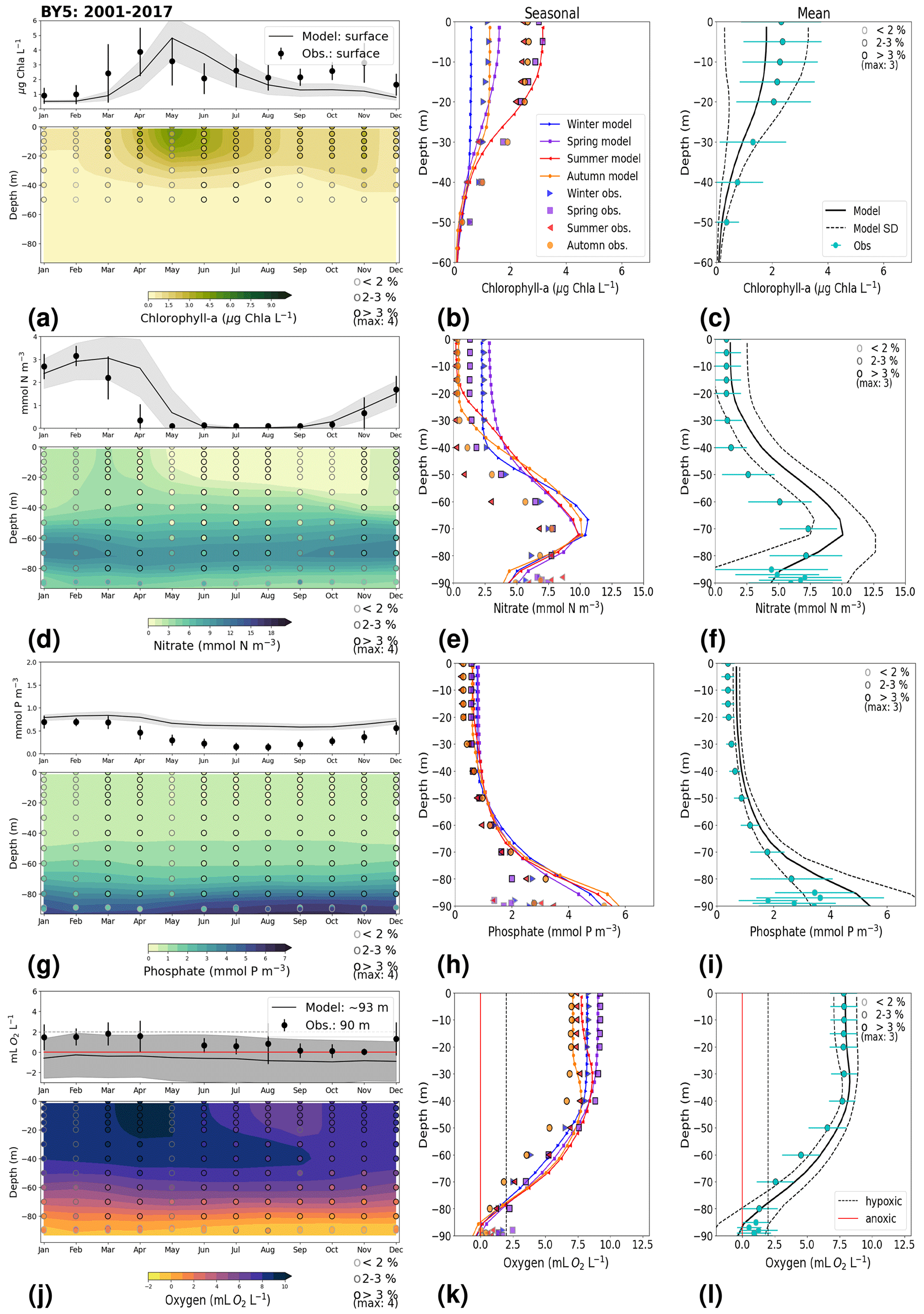
Figure B2Annual and interannual variability in the main biogeochemical parameters at BY5. Detailed description is as in Fig. B1.
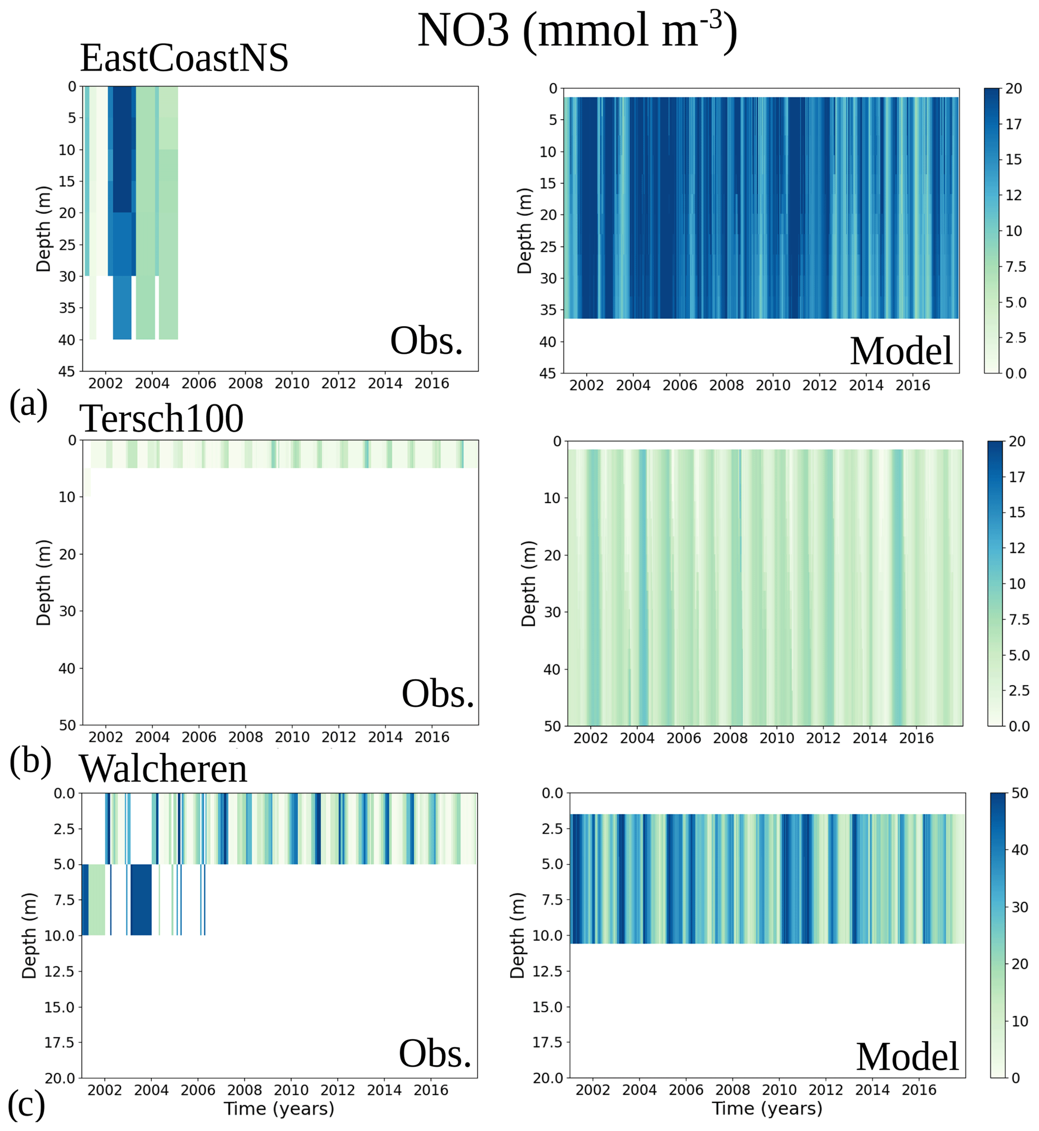
Figure B3Water column nitrate for 2001 to 2017 from observations (left) and the model (right) for three southern North Sea stations: (a) EastCoastNS, (b) Tersh100 and (c) Walcheren. Walcheren is only represented by two vertical layers in the model, as NEMO–SCOBI is not meant to resolve such shallow waters.
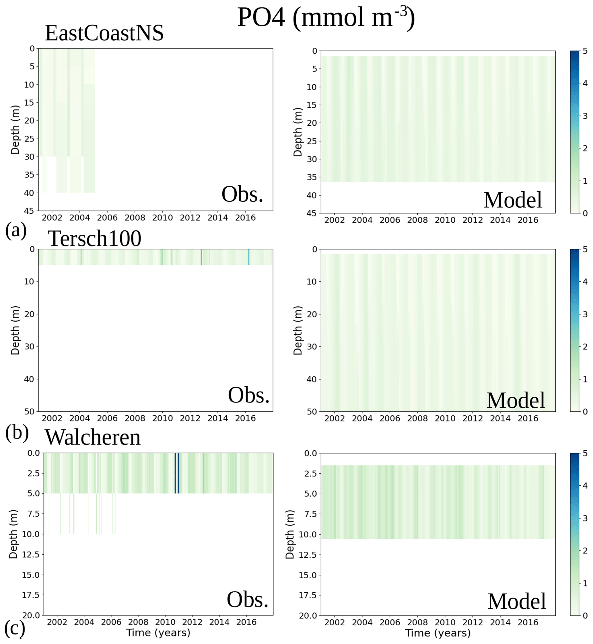
Figure B4Water column phosphate for 2001 to 2017 from observations (left) and the model (right) for three southern North Sea stations: (a) EastCoastNS, (b) Tersh100 and (c) Walcheren.
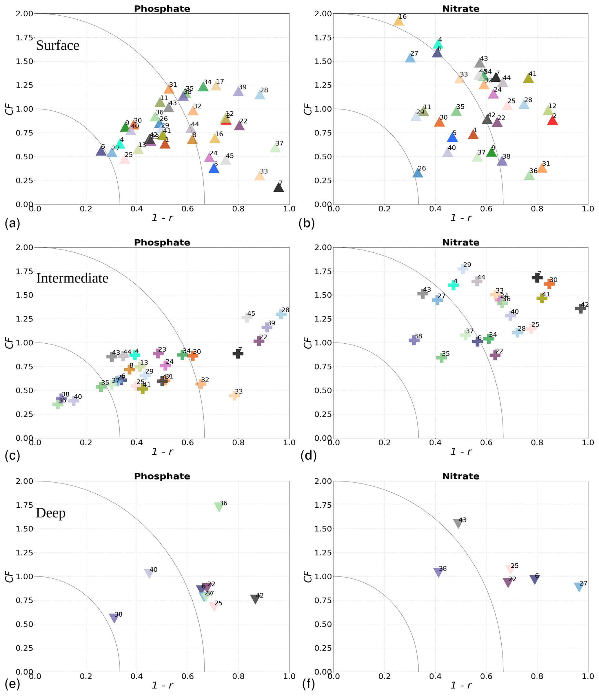
Figure B5Model performance for phosphate and nitrate over the period from 2001 to 2017 shown as a combination of the Pearson correlation bias (1−r) and the cost function bias (CF) for the North Sea–Baltic Sea system evaluated per unit area in Fig. 1 for surface (above 10 m), intermediate (in between 10 and 100 m) and deep (below 100 m) waters. Areas with too few observations are not evaluated (see Sect. 2.2.3).
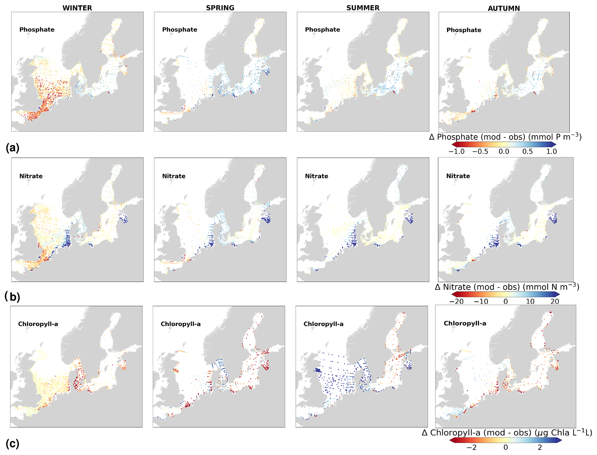
Figure B6The seasonal spatial distribution of the difference between the model results and observations for the period from 2001 to 2017 for PO4, NO3 and chlorophyll a.
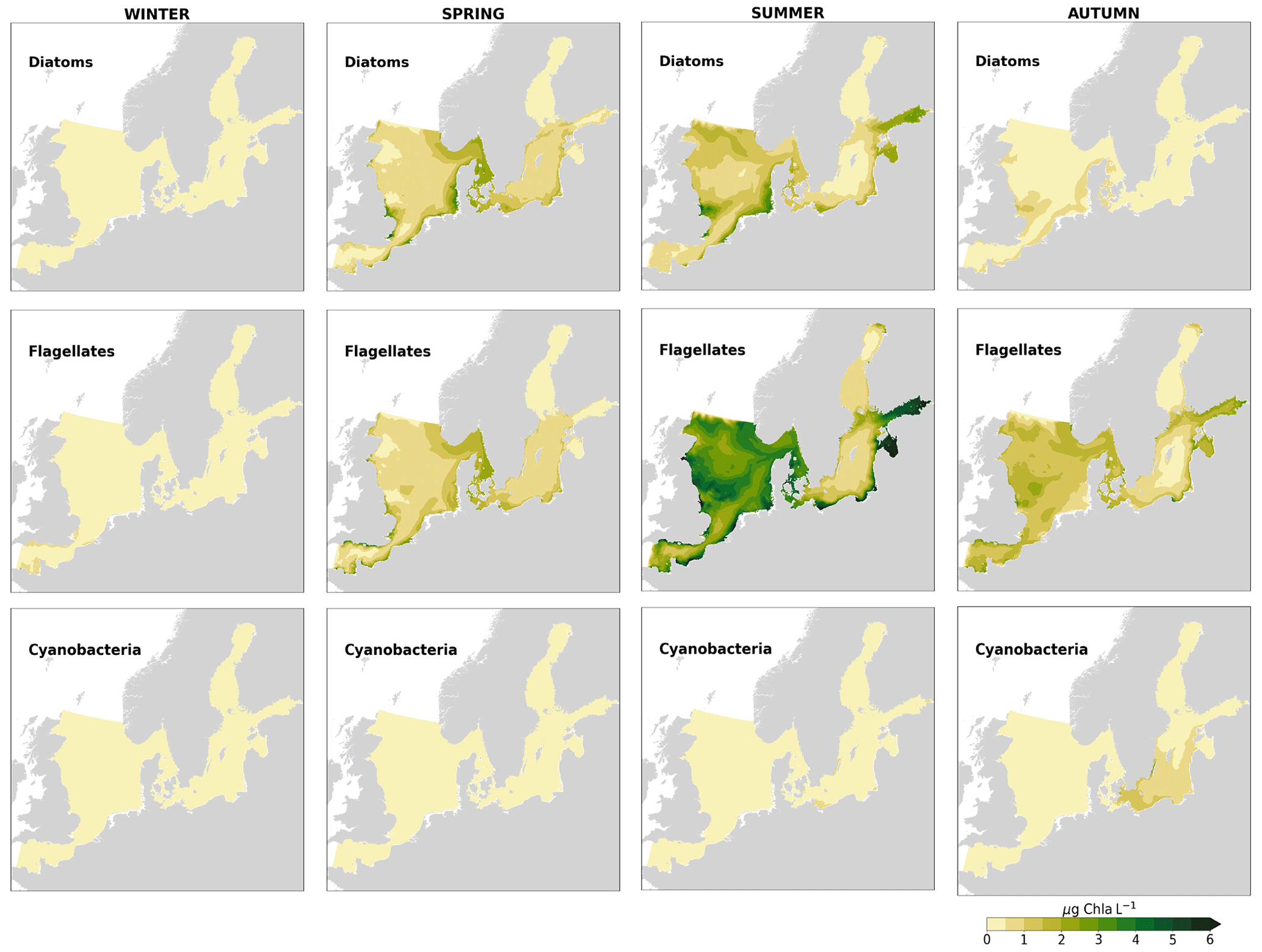
Figure B7Seasonally averaged production by diatoms, flagellates and cyanobacteria in the model for the period from 2001 to 2017.
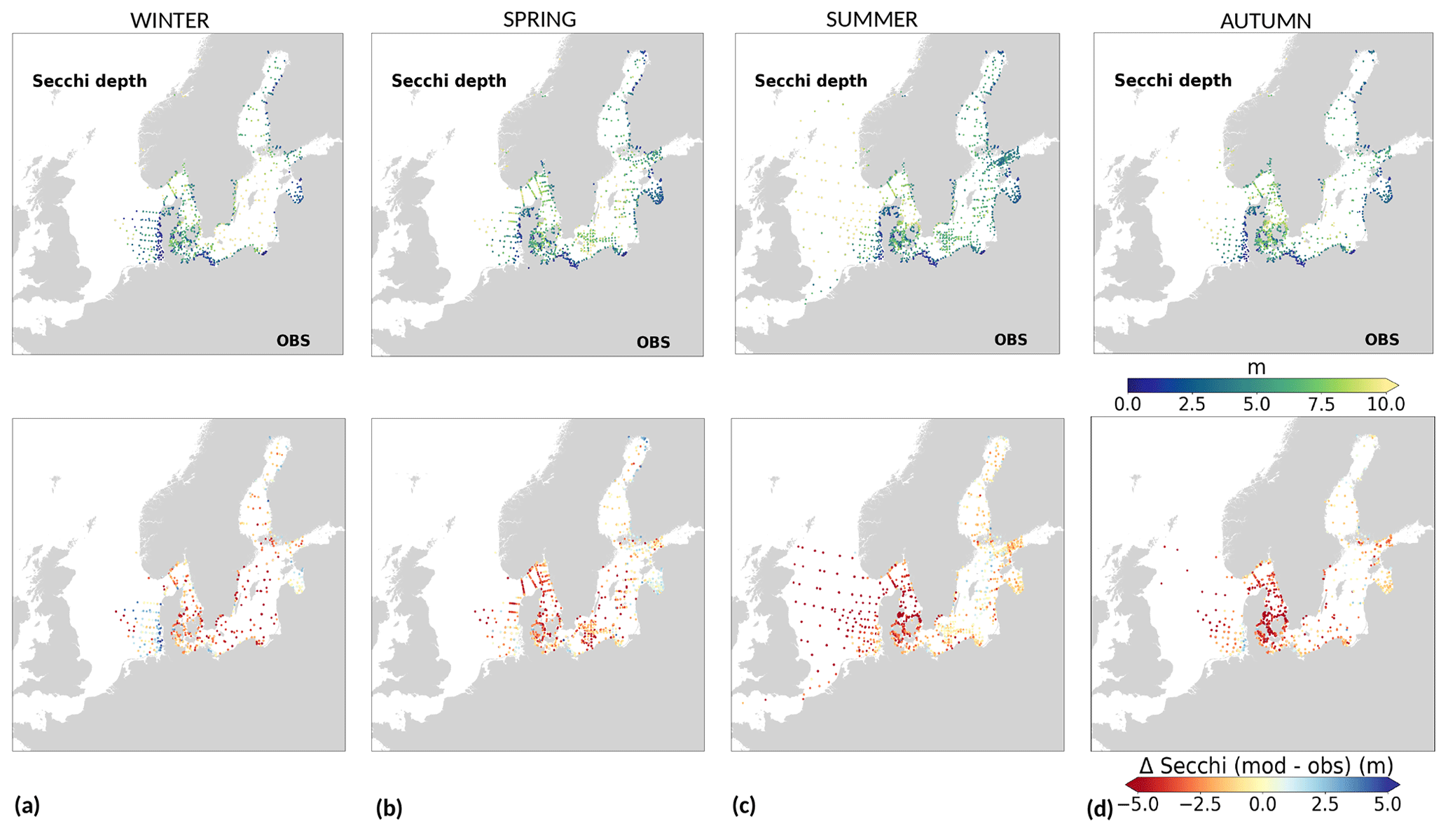
Figure B8Observed light penetration depths shown as averages for (a) winter, (b) spring, (c) summer and (d) autumn for secchi depths and the corresponding differences compared with model values for the period from 2001 to 2017. Modelled secchi depths are approximated as the inverse of the light attenuation coefficient (secchi depth = ).
The NEMO–SCOBI code as applied in this study (NEMO system team and SMHI, 2024) is available upon request by logging into the SMHI GitLab (registration required); https://git.smhi.se/fouo/nemo3.6/-/releases/v2024.03.0.
The river forcing created for and used in this study is described at and freely available from Ruvalcaba Baroni et al. (2024, https://doi.org/10.5281/zenodo.10185658).
IRB, EAR and IK adapted the code of SCOBI to be coupled to NEMO. RH worked on the coupling of NEMO-Nordic to SCOBI. SF and FF set NEMO–SCOBI to the super computer and performed the first tests. IRB, LAr, STF and EAR designed the work. IRB, EAR, SEB, MG, MH, LAx, STF and JH were involved in setting the model forcing and performing and monitoring the run. IRB compiled observations and performed the main analysis work. All authors contributed to discussing and writing the manuscript.
The contact author has declared that none of the authors has any competing interests.
Publisher’s note: Copernicus Publications remains neutral with regard to jurisdictional claims made in the text, published maps, institutional affiliations, or any other geographical representation in this paper. While Copernicus Publications makes every effort to include appropriate place names, the final responsibility lies with the authors.
The authors would like to thank the working groups within OSPAR and HELCOM, in particular the “Intersessional Correspondence Group on Eutrophication Modelling (ICG-EMO)” for regular discussions that supported this work. We are also grateful Kari Eiola and Nathan Grivault for support regarding the technical model details.
This study was funded by the Swedish Agency for Marine and Water Management (HaVs- och vattenmyndigheten; HaVs) within the framework of OSPAR ICG-EMO and “Spring oxygen and chlorophyll-a indicators in the Baltic Sea”. Additional financial support was given by the Swedish government via its climate adaption focus area.
This paper was edited by Perran Cook and reviewed by Tom Jilbert and two anonymous referees.
Almroth, E. and Skogen, M. D.: A North Sea and Baltic Sea model ensemble eutrophication assessment, Ambio, 39, 59–69, https://doi.org/10.1007/s13280-009-0006-7, 2010. a
Almroth-Rosell, E., Eilola, K., Hordoir, R., Meier, H. M., and Hall, P. O.: Transport of fresh and resuspended particulate organic material in the Baltic Sea – a model study, J. Marine Syst., 87, 1–12, https://doi.org/10.1016/j.jmarsys.2011.02.005, 2011. a, b, c, d, e
Almroth-Rosell, E., Eilola, K., Kuznetsov, I., Hall, P. O., and Meier, H. M.: A new approach to model oxygen dependent benthic phosphate fluxes in the Baltic Sea, J. Marine Syst., 144, 127–141, https://doi.org/10.1016/j.jmarsys.2014.11.007, 2015. a, b, c, d, e, f, g, h
Andersen, J. H., Carstensen, J., Conley, D. J., Dromph, K., Fleming-Lehtinen, V., Gustafsson, B. G., Josefson, A. B., Norkko, A., Villnäs, A., and Murray, C.: Long–term temporal and spatial trends in eutrophication status of the Baltic Sea, Biol. Rev., 92, 135–149, https://doi.org/10.1111/brv.12221, 2017. a
Andersson, L.: Trends in nutrients and oxygen concentrations in the Skagerrak-Kattegat, J. Sea Res., 35, 63–71, https://doi.org/10.1016/S1385-1101(96)90735-2, 1996. a, b
Asmala, E., Carstensen, J., Conley, D. J., Slomp, C. P., Stadmark, J., and Voss, M.: Efficiency of the coastal filter: Nitrogen and phosphorus removal in the Baltic Sea, Limnol. Oceanogr., 62, S222–S238, https://doi.org/10.1002/lno.10644, 2017. a, b
Balmaseda, M. A., Mogensen, K., and Weaver, A. T.: Evaluation of the ECMWF ocean reanalysis system ORAS4, Q. J. Roy. Meteor. Soc., 139, 1132–1161, https://doi.org/10.1002/qj.2063, 2013. a
Bartnicki, J., Jonson, J. E., Gauss, M., Nyiri, A., and Klein, H.: Reduction of Atmospheric Nitrogen Deposition to OSPAR Convention Waters Achievable by Implementing Gothenburg Protocol/EU-NEC Directive, OSPAR, https://www.ospar.org/work-areas/hasec/hazardous-substances/camp (last access: January 2024), 2019. a
Beszczynska-Möller, A., Hughes, S. L., and Holliday, N. P.: ICES Report on Ocean Climate, ICES Cooperative Research Reports, https://doi.org/10.17895/ices.pub.5131, 2009. a
Bonaglia, S., Hylén, A., Rattray, J. E., Kononets, M. Y., Ekeroth, N., Roos, P., Thamdrup, B., Brüchert, V., and Hall, P. O. J.: The fate of fixed nitrogen in marine sediments with low organic loading: an in situ study, Biogeosciences, 14, 285–300, https://doi.org/10.5194/bg-14-285-2017, 2017. a
Borja, Á.: The new European Marine Strategy Directive: difficulties, opportunities, and challenges, Mar. Pollut. Bull., 52, 239–242, 2006. a
Burson, A., Stomp, M., Akil, L., Brussaard, C. P., and Huisman, J.: Unbalanced reduction of nutrient loads has created an offshore gradient from phosphorus to nitrogen limitation in the North Sea, Limnol. Oceanogr., 61, 869–888, https://doi.org/10.1002/lno.10257, 2016. a, b, c
Capuzzo, E., Painting, S., Forster, R., Greenwood, N., Stephens, D., and Mikkelsen, O.: Variability in the sub-surface light climate at ecohydrodynamically distinct sites in the North Sea, Biogeochemistry, 113, 85–103, https://doi.org/10.1007/s10533-012-9772-6, 2013. a, b
Capuzzo, E., Stephens, D., Silva, T., Barry, J., and Forster, R. M.: Decrease in water clarity of the southern and central North Sea during the 20th century, Glob. Change Biol., 21, 2206–2214, https://doi.org/10.1111/gcb.12854, 2015. a, b
Carstensen, J. and Conley, D. J.: Frequency, composition, and causes of summer phytoplankton blooms in a shallow coastal ecosystem, the Kattegat, Limnol. Oceanogr., 49, 191–201, https://doi.org/10.4319/lo.2004.49.1.0191, 2004. a, b
Dabuleviciene, T., Vaiciute, D., and Kozlov, I. E.: Chlorophyll-a variability during upwelling events in the south-eastern baltic sea and in the curonian lagoon from satellite observations, Remote Sens., 12, 3661, https://doi.org/10.3390/rs12213661, 2020. a
Daewel, U. and Schrum, C.: Simulating long-term dynamics of the coupled North Sea and Baltic Sea ecosystem with ECOSMO II: Model description and validation, J. Marine Syst., 119, 30–49, https://doi.org/10.1016/j.jmarsys.2013.03.008, 2013. a, b, c, d, e, f, g
Daewel, U. and Schrum, C.: Low-frequency variability in North Sea and Baltic Sea identified through simulations with the 3-D coupled physical–biogeochemical model ECOSMO, Earth Syst. Dynam., 8, 801–815, https://doi.org/10.5194/esd-8-801-2017, 2017. a
Dahlgren, P., Landelius, T., Kållberg, P., and Gollvik, S.: A high-resolution regional reanalysis for Europe. Part 1: Three-dimensional reanalysis with the regional HIgh-Resolution Limited-Area Model (HIRLAM), Q. J. Roy. Meteor. Soc., 142, 2119–2131, https://doi.org/10.1002/qj.2807, 2016. a
Dalsgaard, T., De Brabandere, L., and Hall, P. O.: Denitrification in the water column of the central Baltic Sea, Geochim. Cosmochim. Ac., 106, 247–260, https://doi.org/10.1016/j.gca.2012.12.038, 2013. a, b
Danielssen, D., Edler, L., Fonselius, S., Hernroth, L., Ostrowski, M., Svendsen, E., and Talpsepp, L.: Oceanographic variability in the Skagerrak and northern Kattegat, May–June, 1990, ICES J. Mar. Sci., 54, 753–773, https://doi.org/10.1006/jmsc.1996.0210, 1997. a
Danielsson, Å., Rahm, L., Conley, D., and Carstensen, J.: Identification of characteristic regions and representative stations: a study of water quality variables in the Kattegat, Environ. Monit. Assess., 90, 203–224, https://doi.org/10.1023/B:EMAS.0000003590.58753.0e, 2004. a
Deutsch, B., Forster, S., Wilhelm, M., Dippner, J. W., and Voss, M.: Denitrification in sediments as a major nitrogen sink in the Baltic Sea: an extrapolation using sediment characteristics, Biogeosciences, 7, 3259–3271, https://doi.org/10.5194/bg-7-3259-2010, 2010. a, b
Devlin, M., Fernand, L., and Collingridge, K.: Concentrations of Dissolved Oxygen Near the Seafloor in the Greater North Sea, Celtic Seas and Bay of Biscay and Iberian Coast, in: OSPAR, 2023: The 2023 Quality Status Report for the North-East Atlantic, OSPAR Commission, London, https://oap.ospar.org/en/ospar-assessments/quality-status-reports/qsr-2023/indicator-assessments/seafloor-dissolved-oxygen (last access: January 2024), 2022. a
Donnelly, C., Andersson, J., and Arheimer, B.: Using flow signatures and catchment similarities to evaluate a multi-basin model (E-HYPE) across Europe, Hydrolog. Sci. J., 61, 255–273, https://doi.org/10.1080/02626667.2015.1027710, 2016. a
Döös, K., Meier, H. M., and Döscher, R.: The Baltic haline conveyor belt or the overturning circulation and mixing in the Baltic, Ambio, 33, 261–266, https://doi.org/10.1579/0044-7447-33.4.261, 2004. a, b
Ducrotoy, J.-P. and Elliott, M.: Interrelations between science and policy-making the North Sea example, Mar. Pollut. Bull., 34, 686–701, https://doi.org/10.1016/S0025-326X(97)00118-5, 1997 a
Ducrotoy, J.-P. and Elliott, M.: The science and management of the North Sea and the Baltic Sea: Natural history, present threats and future challenges, Mar. Pollut. Bull., 57, 8–21, https://doi.org/10.1016/j.marpolbul.2008.04.030, 2008. a
Ducrotoy, J.-P., Elliott, M., and de Jonge, V. N.: The North Sea, Mar. Pollut. Bull., 41, 5–23, https://doi.org/10.1016/S0025-326X(00)00099-0, 2000. a, b
Edman, M., Eilola, K., Almroth-Rosell, E., Meier, H., Wåhlström, I., and Arneborg, L.: Nutrient retention in the Swedish coastal zone, Front. Mar. Sci., 5, 415, https://doi.org/10.3389/fmars.2018.00415, 2018. a, b, c, d
Edman, M. K. and Anderson, L. G.: Effect on pCO2 by phytoplankton uptake of dissolved organic nutrients in the Central and Northern Baltic Sea, a model study, J. Marine Syst., 139, 166–182, https://doi.org/10.1016/j.jmarsys.2014.06.004, 2014. a, b
Eilola, K., Meier, H. M., and Almroth, E.: On the dynamics of oxygen, phosphorus and cyanobacteria in the Baltic Sea; A model study, J. Marine Syst., 75, 163–184, https://doi.org/10.1016/j.jmarsys.2008.08.009, 2009. a, b, c, d, e, f, g, h, i, j, k, l, m, n, o, p, q
Eilola, K., Gustafsson, B. G., Kuznetsov, I., Meier, H., Neumann, T., and Savchuk, O.: Evaluation of biogeochemical cycles in an ensemble of three state-of-the-art numerical models of the Baltic Sea, J. Marine Syst., 88, 267–284, https://doi.org/10.1016/j.jmarsys.2011.05.004, 2011a. a, b, c, d, e
Eilola, K., Hansen, J., Meier, M., Myrberg, K., Ryabchenko, V., and Skogen, M.: Eutrophication Status Report of the North Sea, Skagerrak, Kattegat and the Baltic Sea: A Model Study Years 2001–2005, https://www.diva-portal.org/smash (last access: January 2024), 2011b. a
Eilola, K., Rosell, E. A., Dieterich, C., Fransner, F., Höglund, A., and Meier, H.: Modeling nutrient transports and exchanges of nutrients between shallow regions and the open Baltic Sea in present and future climate, Ambio, 41, 586–599, https://doi.org/10.1007/s13280-012-0322-1, 2012. a, b
Feistel, R., Nausch, G., and Wasmund, N. (Eds.): State and evolution of the Baltic Sea, 1952–2005: a detailed 50-year survey of meteorology and climate, physics, chemistry, biology, and marine environment, John Wiley & Sons, ISBN 978-0-471-97968-5, 2008. a, b, c, d
Finni, T., Kononen, K., Olsonen, R., and Wallström, K.: The history of cyanobacterial blooms in the Baltic Sea, Ambio, 30, 172–178, https://doi.org/10.1579/0044-7447-30.4.172, 2001. a
Fonselius, S. H.: Hydrography of the Baltic deep basins, Fiskeristyrelsen, https://www.diva-portal.org/smash (last access: January 2024), 1962. a
Ford, D. A., van der Molen, J., Hyder, K., Bacon, J., Barciela, R., Creach, V., McEwan, R., Ruardij, P., and Forster, R.: Observing and modelling phytoplankton community structure in the North Sea, Biogeosciences, 14, 1419–1444, https://doi.org/10.5194/bg-14-1419-2017, 2017. a, b
Fransner, F., Gustafsson, E., Tedesco, L., Vichi, M., Hordoir, R., Roquet, F., Spilling, K., Kuznetsov, I., Eilola, K., Mörth, C.-M., Humborg, C., and Nycander, J.: Non-Redfieldian dynamics explain seasonal pCO2 drawdown in the Gulf of Bothnia, J. Geophys. Res.-Oceans, 123, 166–188, https://doi.org/10.1002/2017JC013019, 2018. a, b
Gauss, M., Bartnicki, J., Klein, H., and EMEP MSC-W: Atmospheric nitrogen deposition to the Baltic Sea, HELCOM Baltic Sea Environment Fact Sheet (BSEFS), Oslo, https://helcom.fi/wp-content/uploads/2022/12/B_BSEFS_N_dep_v2.pdf (last access: January 2024), 2022. a
Granéli, E., Wallström, K., Larsson, U., Granéli, W., and Elmgren, R.: Nutrient limitation of primary production in the Baltic Sea area, Ambio, 142–151, https://www.jstor.org/stable/4313680 (last access: December 2023), 1990. a
Greenwood, N., Parker, E. R., Fernand, L., Sivyer, D. B., Weston, K., Painting, S. J., Kröger, S., Forster, R. M., Lees, H. E., Mills, D. K., and Laane, R. W. P. M.: Detection of low bottom water oxygen concentrations in the North Sea; implications for monitoring and assessment of ecosystem health, Biogeosciences, 7, 1357–1373, https://doi.org/10.5194/bg-7-1357-2010, 2010. a, b
Gröger, M., Maier-Reimer, E., Mikolajewicz, U., Moll, A., and Sein, D.: NW European shelf under climate warming: implications for open ocean – shelf exchange, primary production, and carbon absorption, Biogeosciences, 10, 3767–3792, https://doi.org/10.5194/bg-10-3767-2013, 2013. a, b
Große, F., Greenwood, N., Kreus, M., Lenhart, H.-J., Machoczek, D., Pätsch, J., Salt, L., and Thomas, H.: Looking beyond stratification: a model-based analysis of the biological drivers of oxygen deficiency in the North Sea, Biogeosciences, 13, 2511–2535, https://doi.org/10.5194/bg-13-2511-2016, 2016. a
Gustafsson, B.: Interaction between Baltic Sea and North Sea, Deutsche Hydrografische Zeitschrift, 49, 165–183, https://doi.org/10.1007/BF02764031, 1997. a, b, c
Gustafsson, B. G., Schenk, F., Blenckner, T., Eilola, K., Meier, H., Müller-Karulis, B., Neumann, T., Ruoho-Airola, T., Savchuk, O. P., and Zorita, E.: Reconstructing the development of Baltic Sea eutrophication 1850–2006, Ambio, 41, 534–548, https://doi.org/10.1007/s13280-012-0318-x, 2012. a, b, c, d, e, f, g
HELCOM: Development of tools for assessment of eutrophication in the Baltic Sea, Baltic Sea Environmental Proceedings No. 104, Helsinki Commission, 64 pp., https://www.helcom.fi (last access: February 2024), 2006. a, b
Henriksen, P.: Long-term changes in phytoplankton in the Kattegat, the Belt Sea, the Sound and the western Baltic Sea, J. Sea Res., 61, 114–123, https://doi.org/10.1016/j.seares.2008.10.003, 2009. a
Hense, I. and Burchard, H.: Modelling cyanobacteria in shallow coastal seas, Ecol. Model., 221, 238–244, https://doi.org/10.1016/j.ecolmodel.2009.09.006, 2010. a
Hieronymus, J., Eilola, K., Olofsson, M., Hense, I., Meier, H. E. M., and Almroth-Rosell, E.: Modeling cyanobacteria life cycle dynamics and historical nitrogen fixation in the Baltic Proper, Biogeosciences, 18, 6213–6227, https://doi.org/10.5194/bg-18-6213-2021, 2021. a
Hieronymus, M., Hieronymus, J., and Hieronymus, F.: On the Application of Machine Learning Techniques to Regression Problems in Sea Level Studies, J. Atmos. Ocean. Tech., 36, 1889–1902, https://doi.org/10.1175/JTECH-D-19-0033.1, 2019. a
Hietanen, S. and Kuparinen, J.: Seasonal and short-term variation in denitrification and anammox at a coastal station on the Gulf of Finland, Baltic Sea, Hydrobiologia, 596, 67–77, https://doi.org/10.1007/s10750-007-9058-5, 2008. a, b
Hietanen, S., Jäntti, H., Buizert, C., Jürgens, K., Labrenz, M., Voss, M., and Kuparinen, J.: Hypoxia and nitrogen processing in the Baltic Sea water column, Limnol. Oceanogr., 57, 325–337, https://doi.org/10.4319/lo.2012.57.1.0325, 2012. a
Holmes, R. W.: The secchi disk in turbid coastal waters 1, Limnol. Oceanogr., 15, 688–694, 1970. a
Holt, J., Butenschön, M., Wakelin, S. L., Artioli, Y., and Allen, J. I.: Oceanic controls on the primary production of the northwest European continental shelf: model experiments under recent past conditions and a potential future scenario, Biogeosciences, 9, 97–117, https://doi.org/10.5194/bg-9-97-2012, 2012. a, b, c, d
Hordoir, R., Axell, L., Löptien, U., Dietze, H., and Kuznetsov, I.: Influence of sea level rise on the dynamics of salt inflows in the Baltic Sea, J. Geophys. Res.-Oceans, 120, 6653–6668, https://doi.org/10.1002/2014JC010642, 2015. a, b, c
Hordoir, R., Axell, L., Höglund, A., Dieterich, C., Fransner, F., Gröger, M., Liu, Y., Pemberton, P., Schimanke, S., Andersson, H., Ljungemyr, P., Nygren, P., Falahat, S., Nord, A., Jönsson, A., Lake, I., Döös, K., Hieronymus, M., Dietze, H., Löptien, U., Kuznetsov, I., Westerlund, A., Tuomi, L., and Haapala, J.: Nemo-Nordic 1.0: a NEMO-based ocean model for the Baltic and North seas – research and operational applications, Geosci. Model Dev., 12, 363–386, https://doi.org/10.5194/gmd-12-363-2019, 2019. a, b, c, d, e, f, g, h, i, j
Huthnance, J., Hopkins, J., Berx, B., Dale, A., Holt, J., Hosegood, P., Inall, M., Jones, S., Loveday, B. R., Miller, P. I., Polton, J., Porter, M., and Spingys, C.: Ocean shelf exchange, NW European shelf seas: Measurements, estimates and comparisons, Prog. Oceanogr., 202, 102760, https://doi.org/10.1016/j.pocean.2022.102760, 2022. a, b
Ikeda, M., Johannessen, J., Lygre, K., and Sandven, S.: A process study of mesoscale meanders and eddies in the Norwegian Coastal Current, J. Phys. Oceanogr., 19, 20–35, https://doi.org/10.1175/1520-0485(1989)019<0020:APSOMM>2.0.CO;2, 1989. a, b, c
Jakobsson, M., Stranne, C., O'Regan, M., Greenwood, S. L., Gustafsson, B., Humborg, C., and Weidner, E.: Bathymetric properties of the Baltic Sea, Ocean Sci., 15, 905–924, https://doi.org/10.5194/os-15-905-2019, 2019. a
Janssen, F., Neumann, T., and Schmidt, M.: Inter-annual variability in cyanobacteria blooms in the Baltic Sea controlled by wintertime hydrographic conditions, Mar. Ecol.-Prog. Ser., 275, 59–68, https://doi.org/10.3354/meps275059, 2004. a, b, c, d, e
Jilbert, T. and Slomp, C. P.: Iron and manganese shuttles control the formation of authigenic phosphorus minerals in the euxinic basins of the Baltic Sea, Geochim. Cosmochim. Ac., 107, 155–169, https://doi.org/10.1016/j.gca.2013.01.005, 2013. a
Kahru, M., Leppänen, J.-M., Rud, O., and Savchuk, O.: Cyanobacteria blooms in the Gulf of Finland triggered by saltwater inflow into the Baltic Sea, Mar. Ecol.-Prog. Ser., 207, 13–18, https://doi.org/10.3354/meps207013, 2000. a
Kenny, A. J., Jenkins, C., Wood, D., Bolam, S. G., Mitchell, P., Scougal, C., and Judd, A.: Assessing cumulative human activities, pressures, and impacts on North Sea benthic habitats using a biological traits approach, ICES J. Mar. Sci., 75, 1080–1092, https://doi.org/10.1093/icesjms/fsx205, 2017. a
Koho, K., Andrusaitis, A., Sirola, M., Ahtiainen, H., Ancans, J., Blauw, A., Cresson, P., Raedemacker, F., Devriese, L., Enserink, L., Gipperth, L., Girardin, R., Herman, P., Hjerpe Olausson, J., Humborg, K., Hyytiäinen, K., Johannesson, K., Lips, U., Kaitaranta, J., Lisbjerg, D., Malde, K., Marchal, P., Martens, C., Mawduk, P., Reeves, S., Riemann, B., Stenseth, N. C., Vandegehuchte, M., Varjopuro, R., von Lukas, U., and Li Zweifel, U.: The Baltic and North Sea Strategic Research and Innovation Agenda, BANOS SRIA 2021, BANOS CSA D, 1, ISBN 978-952-69739-0-6, 2021. a, b, c
Koop, K., Boynton, W. R., Wulff, F., and Carman, R.: Sediment-water oxygen and nutrient exchanges along a depth gradient in the Baltic Sea, Mar. Ecol.-Prog. Ser., 63, 65–77, https://www.jstor.org/stable/24842269 (last access: June 2023), 1990. a
Korpinen, S., Meidinger, M., and Laamanen, M.: Cumulative impacts on seabed habitats: An indicator for assessments of good environmental status, Mar. Pollut. Bull., 74, 311–319, https://doi.org/10.1016/j.marpolbul.2013.06.036, 2013. a
Kuliński, K., Rehder, G., Asmala, E., Bartosova, A., Carstensen, J., Gustafsson, B., Hall, P. O. J., Humborg, C., Jilbert, T., Jürgens, K., Meier, H. E. M., Müller-Karulis, B., Naumann, M., Olesen, J. E., Savchuk, O., Schramm, A., Slomp, C. P., Sofiev, M., Sobek, A., Szymczycha, B., and Undeman, E.: Biogeochemical functioning of the Baltic Sea, Earth Syst. Dynam., 13, 633–685, https://doi.org/10.5194/esd-13-633-2022, 2022. a
Lass, H. and Matthäus, W.: On temporal wind variations forcing salt water inflows into the Baltic Sea, Tellus A, 48, 663–671, https://doi.org/10.1034/j.1600-0870.1996.t01-4-00005.x, 1996. a, b
Lenhart, H.-J., Mills, D. K., Baretta-Bekker, H., van Leeuwen, S. M., van der Molen, J., Baretta, J. W., Blaas, M., Desmit, X., Kühn, W., Lacroix, G., Los, H. J., Ménesguen, A., Neves, R., Proctor, R., Ruardij, P., Skogen, M. D., Vanhoutte-Brunier, A., Villars, M. T., and Wakelin, S. L.: Predicting the consequences of nutrient reduction on the eutrophication status of the North Sea, J. Marine Syst., 81, 148–170, https://doi.org/10.1016/j.jmarsys.2009.12.014, 2010. a, b, c
Leppäranta, M. and Myrberg, K. (Eds.): Physical oceanography of the Baltic Sea, Springer Science & Business Media, ISBN 978-3-540-79702-9, 2009. a
Ly, J., Philippart, C. J., and Kromkamp, J. C.: Phosphorus limitation during a phytoplankton spring bloom in the western Dutch Wadden Sea, J. Sea Res., 88, 109–120, https://doi.org/10.1016/j.seares.2013.12.010, 2014. a, b, c
Maar, M., Møller, E. F., Larsen, J., Madsen, K. S., Wan, Z., She, J., Jonasson, L., and Neumann, T.: Ecosystem modelling across a salinity gradient from the North Sea to the Baltic Sea, Ecol. Model., 222, 1696–1711, https://doi.org/10.1016/j.ecolmodel.2011.03.006, 2011. a, b, c, d, e, f, g
Madec, G., Bourdallé-Badie, R., Bouttier, P.-A., Bricaud, C., Bruciaferri, D., Calvert, D., Chanut, J., Clementi, E., Coward, A., Delrosso, D., Ethé, C., Flavoni, S., Graham, T., Harle, J., Iovino, D., Lea, D., Lévy, C., Lovato, T., Martin, N., Masson, S., Mocavero, S., Paul, J., Rousset, C., Storkey, D., Storto, A., and Vancoppenolle, M.: NEMO ocean engine, Earth Prints, http://hdl.handle.net/2122/13309 (last access: January 2024), 2017. a
Marmefelt, E., Arheimer, B., and Langner, J.: An integrated biogeochemical model system for the Baltic Sea, Hydrobiologia, 393, 45–56, https://doi.org/10.1023/A:1003541816177, 1999. a, b
Mathis, M., Elizalde, A., and Mikolajewicz, U.: The future regime of Atlantic nutrient supply to the Northwest European Shelf, J. Marine Syst., 189, 98–115, https://doi.org/10.1016/j.jmarsys.2018.10.002, 2019. a, b
Mazur-Marzec, H., Żeglińska, L., and Pliński, M.: The effect of salinity on the growth, toxin production, and morphology of Nodularia spumigena isolated from the Gulf of Gdańsk, southern Baltic Sea, J. Appl. Phycol., 17, 171–179, https://doi.org/10.1007/s10811-005-5767-1, 2005. a
McGlade, J. M.: The North Sea Large Marine Ecosystem, in: Large Marine Ecosystems, edited by: Sherman, K. and Skjoldal, H. R., Vol. 10, 339–412, Elsevier, https://doi.org/10.1016/S1570-0461(02)80064-7, 2002. a, b
Mee, L. D., Jefferson, R. L., Laffoley, D. D., and Elliott, M.: How good is good? Human values and Europe's proposed Marine Strategy Directive, Mar. Pollut. Bull., 56, 187–204, https://doi.org/10.1016/j.marpolbul.2007.09.038, 2008. a, b
Meier, H. E. M. and Kauker, F.: Modeling decadal variability of the Baltic Sea: 2, Role of freshwater inflow and large-scale, J. Geophys. Res.-Oceans, 108, 3267, https://doi.org/10.1029/2003JC001797, 2003. a
Meier, H. E. M., Hordoir, R., Andersson, H., Dieterich, C., Eilola, K., Gustafsson, B. G., Höglund, A., and Schimanke, S.: Modeling the combined impact of changing climate and changing nutrient loads on the Baltic Sea environment in an ensemble of transient simulations for 1961–2099, Clim. Dynam., 39, 2421–2441, https://doi.org/10.1007/s00382-012-1339-7, 2012. a, b
Mohrholz, V.: Major Baltic inflow statistics–revised, Front. Mar. Sci., 5, 384, https://doi.org/10.3389/fmars.2018.00384, 2018. a
Mohrholz, V., Naumann, M., Nausch, G., Krüger, S., and Gräwe, U.: Fresh oxygen for the Baltic Sea: An exceptional saline inflow after a decade of stagnation, J. Marine Syst., 148, 152–166, https://doi.org/10.1016/j.jmarsys.2015.03.005, 2015. a
Mort, H. P., Slomp, C. P., Gustafsson, B. G., and Andersen, T. J.: Phosphorus recycling and burial in Baltic Sea sediments with contrasting redox conditions, Geochim. Cosmochim. Ac., 74, 1350–1362, https://doi.org/10.1016/j.gca.2009.11.016, 2010. a
Nausch, M. and Nausch, G.: Bioavailable dissolved organic phosphorus and phosphorus use by heterotrophic bacteria, Aquat. Biol., 1, 151–160, https://doi.org/10.3354/ab00012, 2007. a
NEMO system team and SMHI: Nemo3.6, log in required, GitLab [code], https://git.smhi.se/fouo/nemo3.6/-/releases/v2024.03.0, last access: January 2024. a
Neumann, T., Fennel, W., and Kremp, C.: Experimental simulations with an ecosystem model of the Baltic Sea: a nutrient load reduction experiment, Global Biogeochem. Cy., 16, 7–1, https://doi.org/10.1029/2001GB001450, 2002. a, b
Neumann, T., Radtke, H., Cahill, B., Schmidt, M., and Rehder, G.: Non-Redfieldian carbon model for the Baltic Sea (ERGOM version 1.2) – implementation and budget estimates, Geosci. Model Dev., 15, 8473–8540, https://doi.org/10.5194/gmd-15-8473-2022, 2022. a, b
Olofsson, M., Hagan, J. G., Karlson, B., and Gamfeldt, L.: Large seasonal and spatial variation in nano-and microphytoplankton diversity along a Baltic Sea—North Sea salinity gradient, Sci. Rep., 10, 17666, https://doi.org/10.1038/s41598-020-74428-8, 2020a. a, b
Olofsson, M., Suikkanen, S., Kobos, J., Wasmund, N., and Karlson, B.: Basin-specific changes in filamentous cyanobacteria community composition across four decades in the Baltic Sea, Harmful Algae, 91, 101685, https://doi.org/10.1016/j.hal.2019.101685, 2020b. a, b
Omstedt, A., Elken, J., Lehmann, A., and Piechura, J.: Knowledge of the Baltic Sea physics gained during the BALTEX and related programmes, Prog. Oceanogr., 63, 1–28, https://doi.org/10.1016/j.pocean.2004.09.001, 2004. a, b
OSPAR: OSPAR Integrated Report 2003 on the Eutrophication Status of the OSPAR Maritime Area Based Upon the First Application of the Comprehensive Procedure, OSPAR Commission, 59 pp., ISBN 1-904426-25-5, 2003. a
OSPAR: Revision of the Common Procedure for the Identification of the Eutrophication Status of the OSPAR Maritime Area, Meeting of the OSPAR Commission, 20–24 June 2022, Copenhagen, Denmark, OSPAR 22-08-06 Add.1-2, 2022. a
Otto, L., Zimmerman, J., Furnes, G., Mork, M., Saetre, R., and Becker, G.: Review of the physical oceanography of the North Sea, Neth. J. Sea Res., 26, 161–238, https://doi.org/10.1016/0077-7579(90)90091-T, 1990. a
Paasche, E.: Silicon and the ecology of marine plankton diatoms. II. Silicate-uptake kinetics in five diatom species, Mar. Biol., 19, 262–269, https://doi.org/10.1007/BF02097147, 1973. a
Pasquer, B., Laruelle, G., Becquevort, S., Schoemann, V., Goosse, H., and Lancelot, C.: Linking ocean biogeochemical cycles and ecosystem structure and function: results of the complex SWAMCO-4 model, J. Sea Res., 53, 93–108, https://doi.org/10.1016/j.seares.2004.07.001, 2005. a
Pavelson, J., Kononen, K., and Laanemets, J.: Chlorophyll distribution patchiness caused by hydrodynamical processes: a case study in the Baltic Sea, ICES J. Mar. Sci., 56, 87–99, https://doi.org/10.1006/jmsc.1999.0610, 1999. a
Peeters, J., Los, F., Jansen, R., Haas, H., Peperzak, L., and De Vries, I.: The oxygen dynamics of the Oyster Ground, North Sea. Impact of eutrophication and environmental conditions, Ophelia, 42, 257–288, https://doi.org/10.1080/00785326.1995.10431508, 1995. a
Pemberton, P., Löptien, U., Hordoir, R., Höglund, A., Schimanke, S., Axell, L., and Haapala, J.: Sea-ice evaluation of NEMO-Nordic 1.0: a NEMO–LIM3.6-based ocean–sea-ice model setup for the North Sea and Baltic Sea, Geosci. Model Dev., 10, 3105–3123, https://doi.org/10.5194/gmd-10-3105-2017, 2017. a
Penta, B. and Walsh, J. J.: A one-dimensional ecological model of summer oxygen distributions within the Chukchi Sea, Cont. Shelf Res., 15, 337–356, https://doi.org/10.1016/0278-4343(93)E0006-T, 1995. a
Rantajärvi, E., Olsonen, R., Hällfors, S., Leppänen, J.-M., and Raateoja, M.: Effect of sampling frequency on detection of natural variability in phytoplankton: unattended high-frequency measurements on board ferries in the Baltic Sea, ICES J. Mar. Sci., 55, 697–704, https://doi.org/10.1006/jmsc.1998.0384, 1998. a
Rasmussen, B. and Gustafsson, B.: Computation of nutrient pools and fluxes at the entrance to the Baltic Sea, 1974–1999, Cont. Shelf Res., 23, 483–500, https://doi.org/10.1016/S0278-4343(02)00237-6, 2003. a, b
Reid, P., Lancelot, C., Gieskes, W., Hagmeier, E., and Weichart, G.: Phytoplankton of the North Sea and its dynamics: a review, Neth. J. Sea Res., 26, 295–331, https://doi.org/10.1016/0077-7579(90)90094-W, 1990. a
Reinart, A. and Kutser, T.: Comparison of different satellite sensors in detecting cyanobacterial bloom events in the Baltic Sea, Remote Sens. Environ., 102, 74–85, https://doi.org/10.1016/j.rse.2006.02.013, 2006. a
Reissmann, J. H., Burchard, H., Feistel, R., Hagen, E., Lass, H. U., Mohrholz, V., Nausch, G., Umlauf, L., and Wieczorek, G.: Vertical mixing in the Baltic Sea and consequences for eutrophication–A review, Prog. Oceanogr., 82, 47–80, https://doi.org/10.1016/j.pocean.2007.10.004, 2009. a
Rönnberg, C. and Bonsdorff, E.: Baltic Sea eutrophication: area-specific ecological consequences, Hydrobiologia, 514, 227–241, https://doi.org/10.1023/B:HYDR.0000019238.84989.7f, 2004. a
Ruvalcaba Baroni, I., Axell, L., Almroth-Rosell, E., Saraiva, S., Mulder, E., Brunnabend, S.-E., Fredriksson, S. T., Bartosova, A., Capell, R., and Arneborg, L.: Daily runoff and nutrient loads for the North Sea and the Baltic Sea based on modelling and observations for the period 1961 to 2019 and adapted to NEMO-SCOBI, Zenodo [data set], https://doi.org/10.5281/zenodo.10185658, 2024. a, b, c, d
Rydberg, L., Ærtebjerg, G., and Edler, L.: Fifty years of primary production measurements in the Baltic entrance region, trends and variability in relation to land-based input of nutrients, J. Sea Res., 56, 1–16, https://doi.org/10.1016/j.seares.2006.03.009, 2006. a
Savchuk, O. P., Wulff, F., Hille, S., Humborg, C., and Pollehne, F.: The Baltic Sea a century ago – a reconstruction from model simulations, verified by observations, J. Marine Syst., 74, 485–494, https://doi.org/10.1016/j.jmarsys.2008.03.008, 2008. a, b
Savchuk, O. P., Gustafsson, B. G., and Müller-Karulis, B.: BALTSEM – a marine model for decision support within the Baltic Sea Region, Baltic Nest Institute, Technical report N.7, urn:nbn:se:su:diva-197187, 2012. a, b
She, J., Berg, P., and Berg, J.: Bathymetry impacts on water exchange modelling through the Danish Straits, J. Marine Syst., 65, 450–459, https://doi.org/10.1016/j.jmarsys.2006.01.017, 2007. a
Siiriä, S.-M., Fredriksson, S., Haapala, J., and Arneborg, L.: The future of Gulf of Bothnia, possible changes on salinity and currents, EGU General Assembly 2022, Vienna, Austria, 23–27 May 2022, EGU22-8533, https://doi.org/10.5194/egusphere-egu22-8533, 2022. a
Stigebrandt, A.: A model for the vertial circulation of the Baltic deep water, J. Phys. Oceanogr., 17, 1772–1785, https://doi.org/10.1175/1520-0485(1987)017<1772:AMFTVC>2.0.CO;2, 1987. a
Stockenberg, A. and Johnstone, R.: Benthic denitrification in the Gulf of Bothnia, Estuar. Coast. Shelf S., 45, 835–843, https://doi.org/10.1006/ecss.1997.0271, 1997. a
Sündermann, J. and Pohlmann, T.: A brief analysis of North Sea physics, Oceanologia, 53, 663–689, https://doi.org/10.5697/oc.53-3.663, 2011. a, b, c
Thamatrakoln, K. and Hildebrand, M.: Silicon uptake in diatoms revisited: a model for saturable and nonsaturable uptake kinetics and the role of silicon transporters, Plant Physiol., 146, 1397–1407, https://doi.org/10.1104/pp.107.107094, 2008. a
Thompson, C., Couceiro, F., Fones, G., Helsby, R., Amos, C., Black, K., Parker, E., Greenwood, N., Statham, P., and Kelly-Gerreyn, B.: In situ flume measurements of resuspension in the North Sea, Estuar. Coast. Shelf S., 94, 77–88, https://doi.org/10.1016/j.ecss.2011.05.026, 2011. a
Tuominen, L., Heinänen, A., Kuparinen, J., and Nielsen, L. P.: Spatial and temporal variability of denitrification in the sediments of the northern Baltic Proper, Mar. Ecol.-Prog. Ser., 172, 13–24, https://doi.org/10.3354/meps172013, 1998. a, b
Van der Molen, J.: The influence of tides, wind and waves on the net sand transport in the North Sea, Cont. Shelf Res., 22, 2739–2762, https://doi.org/10.1016/S0278-4343(02)00124-3, 2002. a
van Leeuwen, S., Tett, P., Mills, D., and van der Molen, J.: Stratified and nonstratified areas in the North Sea: Long-term variability and biological and policy implications, J. Geophys. Res.-Oceans, 120, 4670–4686, https://doi.org/10.1002/2014JC010485, 2015. a, b, c, d, e
van Leeuwen, S. M., Lenhart, H.-J., Prins, T. C., Blauw, A., Desmit, X., Fernand, L., Friedland, R., Kerimoglu, O., Lacroix, G., van der Linden, A., Lefebvre, A., van der Molen, J., Plus, M., Ruvalcaba Baroni, I., Silva, T., Stegert, C., Troost, T. A., and Vilmin, L.: Deriving pre-eutrophic conditions from an ensemble model approach for the North-West European seas, Front. Mar. Sci., 10, 1129951, https://doi.org/10.3389/fmars.2023.1129951, 2023. a, b, c, d, e
Vermaat, J. E., McQuatters-Gollop, A., Eleveld, M. A., and Gilbert, A. J.: Past, present and future nutrient loads of the North Sea: causes and consequences, Estuar. Coast. Shelf S., 80, 53–59, https://doi.org/10.1016/j.ecss.2008.07.005, 2008. a
Wåhlström, I., Höglund, A., Almroth-Rosell, E., MacKenzie, B. R., Gröger, M., Eilola, K., Plikshs, M., and Andersson, H. C.: Combined climate change and nutrient load impacts on future habitats and eutrophication indicators in a eutrophic coastal sea, Limnol. Oceanogr., 65, 2170–2187, https://doi.org/10.1002/lno.11446, 2020. a
Winther, N. G. and Johannessen, J. A.: North Sea circulation: Atlantic inflow and its destination, J. Geophys. Res.-Oceans, 111, C12018, https://doi.org/10.1029/2005JC003310, 2006. a, b, c
Wulff, F. and Stigebrandt, A.: A time-dependent budget model for nutrients in the Baltic Sea, Global Biogeochem. Cy., 3, 63–78, https://doi.org/10.1029/GB003i001p00063, 1989. a
Wulff, F., Rahm, L., Hallin, A.-K., and Sandberg, J.: A nutrient budget model of the Baltic Sea, A systems analysis of the Baltic Sea, edited by: Wulff, F. V., Rahm, L. A., and Larsson, P., Springer, 353–372, https://doi.org/10.1007/978-3-662-04453-7_13, 2001. a
- Abstract
- Introduction
- Material and methods
- Results and discussion
- Conclusions
- Appendix A: Additional NEMO–SCOBI parameterizations
- Appendix B: Additional results
- Code availability
- Data availability
- Author contributions
- Competing interests
- Disclaimer
- Acknowledgements
- Financial support
- Review statement
- References