the Creative Commons Attribution 4.0 License.
the Creative Commons Attribution 4.0 License.
 | 16 Jan 2024
Coupling numerical models of deltaic wetlands with AirSWOT, UAVSAR, and AVIRIS-NG remote sensing data
Carmine Donatelli
Xiaohe Zhang
Justin A. Nghiem
Marc Simard
Cathleen E. Jones
Michael Denbina
Cédric G. Fichot
Joshua P. Harringmeyer
Sergio Fagherazzi
Coastal marsh survival relies on the ability to increase elevation and offset sea level rise. It is therefore important to realistically model sediment fluxes between marshes, tidal channels, and bays as sediment availability controls accretion. Traditionally, numerical models have been calibrated and validated using in situ measurements at a few locations within the domain of interest. These datasets typically provide temporal information but lack spatial variability. This paper explores the potential of coupling numerical models with high-resolution remote sensing imagery. Products from three sensors from the NASA Delta-X airborne mission are used. Uninhabited Aerial Vehicle Synthetic Aperture Radar (UAVSAR) provides vertical water level change on the marshland and was used to adjust the bathymetry and calibrate water fluxes over the marsh. AirSWOT yields water surface elevation within bays, lakes, and channels, and was used to calibrate the Chezy bottom friction coefficient. Finally, imagery from AVIRIS-NG provides maps of total suspended solids (TSS) concentration that were used to calibrate sediment parameters of settling velocity and critical shear stress for erosion. Three numerical models were developed at different locations along coastal Louisiana using Delft3D. The coupling enabled a spatial evaluation of model performance that was not possible using simple point measurements. Overall, the study shows that calibration of numerical models and their general performance will greatly benefit from remote sensing.
- Article
(13081 KB) - Full-text XML
-
Supplement
(13485 KB) - BibTeX
- EndNote


Coastal marshes are among the most important and functional ecosystems on Earth, as they are able to buffer and protect from storm surges and winds (Farber, 1987; Möller et al., 2014; Haddad et al., 2016; Peter Sheng et al., 2022; Temmerman et al., 2023), store carbon (Saintilan et al., 2013; Nahlik and Fennessy, 2016; Rogers et al., 2019), and offer natural habitat to wildlife (Galbraith et al., 2002; Minello et al., 2003). However, it has been estimated that since the 1900s around 50 % of coastal wetlands have been lost (Nicholls, 2004). The resilience of present coastal wetlands is altered by accelerated sea level rise (Cahoon et al., 2006; Spencer et al., 2016; Schuerch et al., 2018), enhanced subsidence due to groundwater and oil extraction (Syvitski et al., 2009), and depleted sediment supply to the coast as a result of extensive river damming (Syvitski et al., 2005). Physically based models are necessary to understand and predict the response of coastal wetlands to such external drivers (Fagherazzi et al., 2020).
Incoming and outgoing sediment fluxes are key for the evolution of coastal marshes in a climate change scenario (Ganju et al., 2017). Consequently, it is imperative that numerical models accurately solve the hydrodynamic and sediment transport processes in the coastal area. Currently, scientists use stations that measure local parameters such as water levels, temperature, salinity, and sediment concentration to validate physical models of coastal marshes. This approach is shared by modeling studies that focus solely on hydrodynamics (e.g., Dietrich et al., 2011; Bunya et al., 2010; Defne and Ganju, 2015) and studies that include sediment transport (e.g., Castagno et al., 2018; Zang et al., 2018; Zhang et al., 2019). In most cases, the instrumentation is installed in a few locations in the open sea, along the coastline, or within tidal channels and creeks, as sensor installation becomes challenging on the shallow coastal marshes where boat access is difficult. Furthermore, these in situ measurements inform about temporal variability, but provide limited spatial information across the landscape. Consequently, it is challenging to fully evaluate the quality of numerical simulations over the marsh platform, which must capture the flux of water and sediment. Despite recent progress in this direction, there remains a need to include the extensive information provided by remote sensing imagery in numerical models (Fagherazzi et al., 2020).
Over time, the introduction of more advanced sensors has improved the spatial resolution of available remote sensing imagery. Coarser resolution sensors, including the Moderate Resolution Imaging Spectroradiometer (MODIS) and the National Oceanic and Atmospheric Administration (NOAA) Advanced Very High-Resolution Radiometer (AVHRR) have been used in various wetlands studies. MODIS data have the advantage of providing near daily coverage of the Earth’s surface, but with a resolution of 250 or 500 m depending on the selected band (Pflugmacher et al., 2007). MODIS data time series have been used to monitor wetland cover (Tana et al., 2013), estuarine vegetation succession and tidal flat elevation (Zhao et al., 2009), tidal wetlands biophysical characteristics (Ghosh et al., 2016), hurricane disturbance to coastal vegetation (Wang and D'Sa, 2009), and coastal wetland biomass (Lumbierres et al., 2017). MODIS data have also been coupled with tower-based flux measurements to determine the carbon budget and the gross primary production in estuarine and coastal wetlands (Yan et al., 2008; Kang et al., 2018). Similar to MODIS, AVHRR provides global imagery twice a day, but with a 1 km resolution. AVHRR data applications vary from assessing hurricane damage in wetlands (e.g., Ill et al., 1997) to the Normalized Difference Vegetation Index (NDVI) seasonal pattern in deltaic systems (e.g., Zoffoli et al., 2008).
Moderate spatial resolution sensors, with spatial resolution of tens of meters, provide much greater detail of the Earth’s surface than MODIS and AVHRR. Among them, data provided by the Landsat and Sentinel sensors have been used to monitor coastal wetlands more often than other sensors such as the Advanced Spaceborne Thermal Emission and Reflection Radiometer, China & Brazil Earth Resource Satellite, Systeme Probatoire D'Observation De La Terre (SPOT 1–4), and Advanced Land Observing Satellite (ALOS) (Guo et al., 2017). Long-term Landsat time series have been used to detect coastal wetlands cover and area change (Cardoso et al., 2014; Couvillion et al., 2017; Kaplan and Avdan, 2017; Wang et al., 2019, 2020), wetlands vegetation classification and change (Zhang et al., 2011, 2022c; Muro et al., 2016; Lopes et al., 2019; Thomas et al., 2019; Balogun et al., 2020), extreme events impact on vegetation (Rodgers et al., 2009), coastal wetland soil vertical accretion rates (Jensen et al., 2022), and coastal wetland above-ground biomass (Tan et al., 2003; Chen et al., 2022).
Remote sensing studies have also developed algorithms to infer water quality indicators in coastal waters near wetlands (McClain and Meister, 2012). For instance, Fichot et al. (2016) used high-resolution remote-sensing reflectance data from the airborne Portable Remote Sensing Spectrometer to derive maps of turbidity, dissolved organic carbon and chlorophyll-a in the San Francisco Bay-Delta Estuary. Jensen et al. (2019) used high-resolution remote-sensing reflectance data from NASA’s Airborne Visible-Infrared Imaging Spectrometer-Next Generation (AVIRIS-NG) to derive maps of total surface-suspended solids in the waters of the Atchafalaya basin along the Louisiana coast (USA). They used an algorithm centered on a derivative-based partial least squares regression between measured total surface suspended solids and in situ spectra. Other studies utilized operational satellite sensors with coarser spatial resolution and fewer spectral bands to derive sediment concentrations in coastal waters. Dorji and Fearns (2016) applied multiple algorithms to MODIS and Landsat imagery in regional waters of northern Western Australia, whereas Zhang et al. (2020a) adopted Landsat-8 and Sentinel-2 imagery to derive suspended sediment concentration in Plum Island Estuary in Massachusetts (USA).
High-quality optical imagery is limited to cloud-free conditions; therefore, remote sensing techniques can also rely on radar sensors to overcome this limitation (Henderson and Lewis, 2008). The ALOS Phased Array L-band Synthetic Aperture Radar, European Remote Sensing satellite, RadarSAT, Advanced Synthetic Aperture Radar, Japanese Earth Resources Satellite 1, Airborne Synthetic Aperture Radar (AIRSAR), and TerraSAR-X are some examples of radar sensors used to monitor wetlands (Guo et al., 2017). Slatton et al. (2008) showed that changes in the multi-polarization L-band AIRSAR backscatter were able to detect herbaceous vegetation in marshes, whereas Kwoun and Lu (2009) used SAR data over the Louisiana coastal zone to characterize seasonal variations of radar backscattering according to vegetation type. These studies show that SAR can be adopted to monitor changes in coastal wetland vegetation cover. Within the last decade repeat-pass radar interferometry from spaceborne instruments have enabled measurements of water-level change within marshes (Wdowinski et al., 2008; Liao et al., 2020; Xie et al., 2013; Hong and Wdowinski, 2014). This new technology enables direct observation of large-scale flow patterns that can only be observed with remote sensing.
This study presents a novel coupling between numerical modeling and high-resolution remote sensing imagery. In particular, it shows that the calibration of hydrological and sediment transport models can be performed with multiple remote sensing data. To do so, three remote sensing products from the NASA Delta-X mission are used to inform three numerical models with different spatial resolutions. The paper is structured in the following sections: an introduction to the Delta-X mission and related remote sensing products, set-up of the numerical models, results, and discussion of advantages and limitations of using these datasets with numerical models.
2.1 Study area and models domains
The Terrebonne and Atchafalaya basins are two neighboring coastal basins located along the Louisiana coast, to the west of the Mississippi River birdfoot delta (Fig. 1). Among all basins in the Mississippi River Delta Plain (MRDP), the Terrebonne wetlands have seen the highest rate of areal loss since 1932 (Couvillion et al., 2017; Jensen et al., 2022) owing to a lack of sediment load from inland waters. Furthermore, because of the microtidal environment, mineral soil accretion heavily relies on wind waves for bottom sediment resuspension and on storm surges to transport the sediment over the marsh platform (Cortese and Fagherazzi, 2022). The basin is characterized by a strong salinity gradient, with salt marshes dominated by Spartina alterniflora along the coast, and brackish and fresh marshes located in landward areas (Twilley et al., 2019).
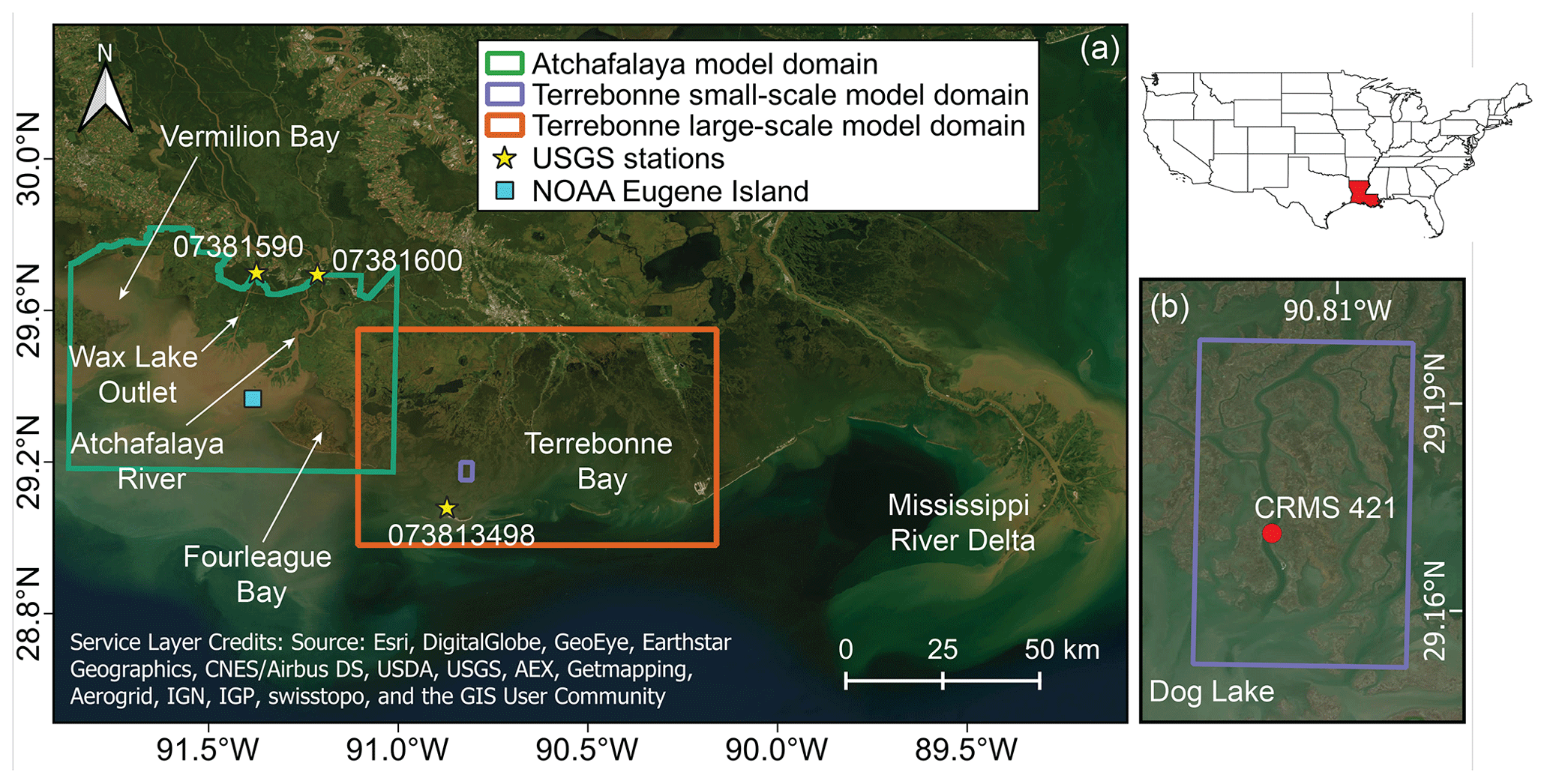
Figure 1(a) The domains for the Atchafalaya and Terrebonne basin numerical models. The top left inset shows a map of the contiguous USA with the state of Louisiana colored in red. (b) Inset showing a detail of the small-scale model domain in the Terrebonne basin. Sources for satellite images in Fig. 1b are: Esri, DigitalGlobe, GeoEye, Earthstar Geographics, CNES/Airbus DS, USDA, AEX, Getmapping, Aerogrid, IGN, IGP, swisstopo, and the GIS User Community.
The Atchafalaya basin is located west of Terrebonne and includes the Atchafalaya River and the Wax Lake Outlet. Both rivers mirror the seasonal pattern of the Mississippi hydrograph, with peak discharge between January and June and low discharge in September and October (Allison et al., 2000). The two rivers receive around 30 % of the Mississippi River flow through the Old River Control floodgate located north of Baton Rouge (Roberts et al., 2003) and have actively growing deltas, representing a rare instance of land gain along Louisiana’s coast (Couvillion et al., 2017). For instance, the Wax Lake Delta has prograded seaward at a 270 m yr−1 rate between 1980 and 2002 (Parker and Sequeiros, 2006). In the Atchafalaya basin nearly 80 % of the wetlands are freshwater marshes and swamps owing to the high freshwater discharge (Twilley et al., 2019). The distribution of the vegetation is heavily regulated by topography and hydroperiod (Bevington and Twilley, 2018).
Three numerical models were developed at different scales and calibrated with remote sensing data. Two models were set-up on the basin scale, whereas the third one was developed on a smaller scale. The large-scale Terrebonne model (red rectangle in Fig. 1) extends longitudinally for 90 km and borders with the Atchafalaya basin to the west. The small-scale Terrebonne model is located within the salt marsh in the south-west portion of Terrebonne (blue rectangle in Fig. 1) and is connected to the south by Dog Lake. The domain consists of an island surrounded by two main channels with a 100–150 m wide cross section that converge at the northern top of the island. Finally, the Atchafalaya model (green rectangle in Fig. 1) extends longitudinally for 84 km and includes the two deltas, Fourleague Bay to the east, and Vermilion Bay to the west.
2.2 NASA Delta-X mission
Delta-X is a NASA mission funded by the Science Mission Directorate’s Earth Science Division through the Earth Venture Suborbital-3 Program (Simard et al., 2022; https://deltax.jpl.nasa.gov/, last access: 20 October 2023), which investigates how feedback between hydrological and ecological processes enables marshes and deltas to survive the relative sea level rise. The project is focused on the two basins of the MRDP introduced above. The mission has produced airborne high-resolution remote sensing imagery and in situ measurements that can be incorporated in hydrodynamic, sediment transport, and ecological numerical models. In 2021, two field campaigns were completed, one in Spring and one in Fall in order to capture the maximum and minimum flood stages of the Mississippi river discharge.
2.3 UAVSAR, AirSWOT, and AVIRIS-NG
During both Delta-X campaigns, three airborne remote sensing instruments repeatedly collected data to capture the hydrological parameters and infer sediment concentration during different tidal stages.
The Uninhabited Aerial Vehicle Synthetic Aperture Radar (UAVSAR) is a fully polarimetric L-band synthetic aperture radar (SAR) with a wavelength of 23.8 cm, installed on a NASA Gulfstream-III aircraft, that can provide highly coherent rapid repeat-pass SAR acquisitions. UAVSAR data provide a measurement of water-level change over the wetlands with a resolution of 6 m through repeat-pass interferometry, which allows the detection of surface displacement using multiple observations from the same viewing geometry (Rosen et al., 2006). In flooded wetlands, the water surface is detected through the double-bounce scattering mechanism from water and vegetation (Kim et al., 2009; Wdowinski et al., 2013). To separate the water surface from the emergent wetland, a water mask was generated from the interferogram Level-1 products. Figure 2a shows an example of water- level change measured by UAVSAR on the wetlands in western Terrebonne between 17:13 and 17:44 (GMT) on 6 April 2021. A phase unwrapping algorithm is employed to convert interferometric phase change Δϕ to change in elevation Δz (Oliver-Cabrera et al., 2021). Here, Level-3 UAVSAR data acquired in Terrebonne are used (Jones et al., 2022).
AirSWOT is an airborne Ka-band synthetic aperture radar with a wavelength of 0.84 cm flown on a Beechcraft King Air B200, that measures water-surface elevation and water-surface slope in open waters with uncertainty below 0.3 cm km−1. AirSWOT uses cross-track interferometry to measure the elevation and combines it with along-track interferometry to correct for the bias due to the water motion (Goldstein and Zebker, 1987). To separate land from water surfaces, the same UAVSAR water mask was used for AirSWOT. More details on the application of AirSWOT are reported by Denbina et al. (2019). Figure 2b shows an example of water-surface elevation in western Terrebonne acquired along a flight line on 5 April 2021 at 22:22 GMT. Here, Level-2 AirSWOT geocoded water-surface elevation data in Terrebonne and Wax Lake (Denbina et al., 2022) are used. Water-surface elevation data were validated in both Delta-X campaigns using in situ gauges and a root mean squared error of 9 cm was found when data were averaged on a 1 km2 area.
The Airborne Visible-Infrared Imaging Spectrometer-Next Generation (AVIRIS-NG) is a high-resolution imaging spectrometer that measures radiance for 432 bands at 5 nm spectral sampling between 380 and 2510 nm (Hamlin et al., 2011). The calibrated radiance measurements from AVIRIS-NG were atmospherically corrected to produce spectral remote-sensing reflectance (Rrs(λ)) of the water, and surface reflectance of the land. Local empirical algorithms derived using in situ measurements were used to derive TSS concentration from the Rrs(λ) in the visible and near-infrared region and generate maps of TSS from the AVIRIS-NG imagery (Gao et al., 1993; Bue et al., 2015; Jensen et al., 2019). In situ samples were collected in both Terrebonne and Atchafalaya basins during the Delta-X 2021 Spring and Fall campaigns in order to capture high- and low-flow conditions. The algorithm to retrieve TSS from AVIRIS-NG performed well (Median Absolute Percent Difference 13.7 % and Median bias 6.71 mg L−1) across a wide range of TSS concentrations (0.1–154.5 mg L−1) (Fichot and Harringmeyer, 2021, 2022). AVIRIS-NG images were also used to produce maps of vegetation structure (Jensen et al., 2021). Figure 2c shows an example of total suspended solids (TSS) concentration maps derived from AVIRIS-NG over the Wax Lake Outlet acquired on 2 April 2021 at 20:31 GMT. Here, the AVIRIS-NG Level3-derived TSS data in Terrebonne and Wax Lake are used (Fichot and Harringmeyer, 2022).
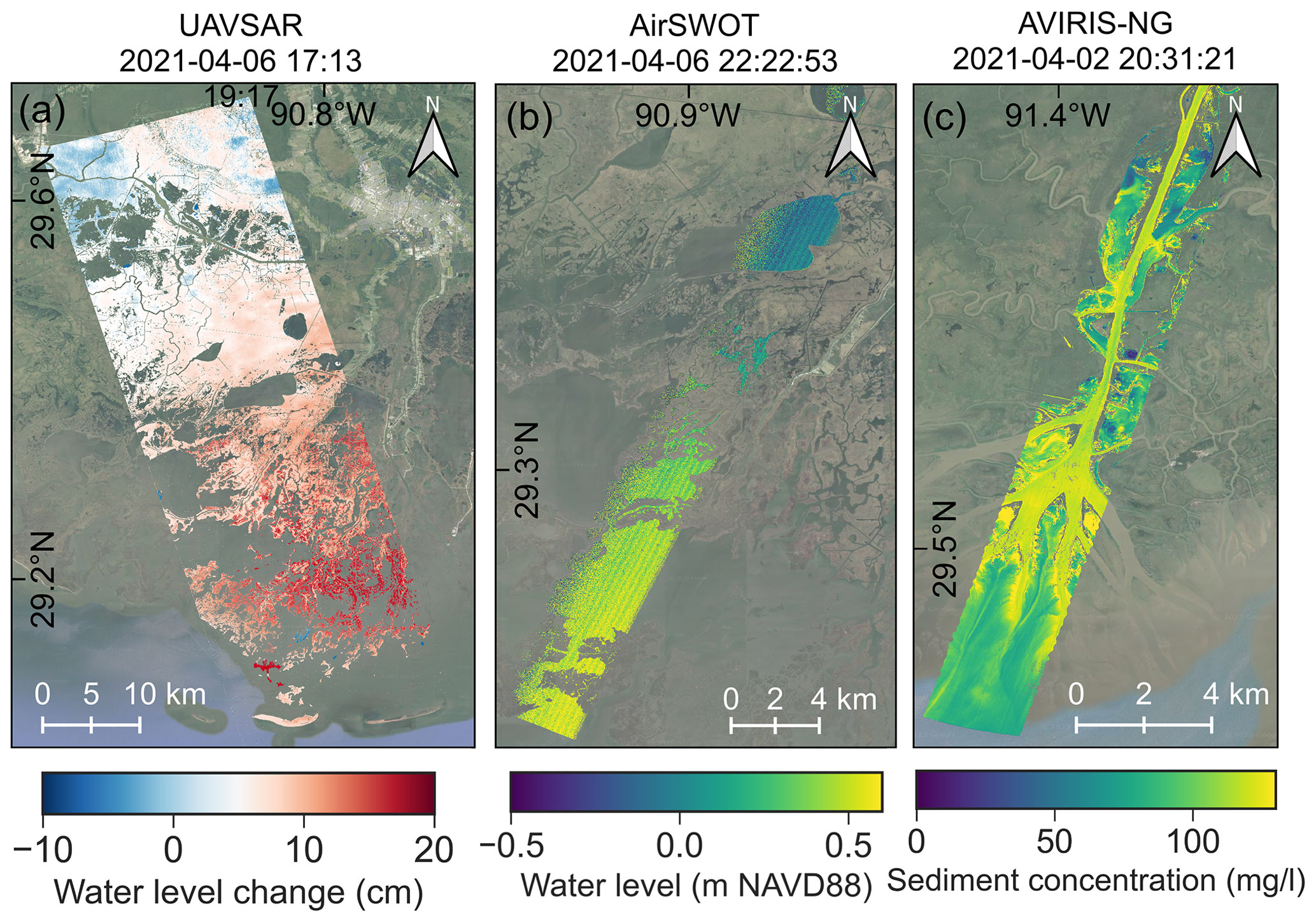
Figure 2Example of Delta-X remote sensing products. At the top of each map the acquisition time is reported in GMT. (a) Water-level change on the marsh from UAVSAR. (b) Water elevation from AirSWOT. (c) Total suspended solids (TSS) concentration derived from AVIRIS-NG. Refer to Fig. 3 for the spatial relationship. Basemap credits: © Google Satellite.
2.4 Large-scale Terrebonne model set-up
The Delft3D model was used to simulate water levels and sediment transport during the Delta-X 2021 Spring campaign. The FLOW module (Lesser et al., 2004) was coupled with SWAN (Simulating Waves Nearshore, e.g. Holthuijsen et al., 1993; Booij and Holthuijsen, 1987) to account for wave resuspension of bottom sediments. The model ran from 25 March to 18 April 2021 with an additional 5 d as a spin-up period. The domain (Fig. 1) consisted of 1139×686 cells with a 90×90 m resolution. Bathymetric data were referenced to the NAVD88 vertical datum and are available from the NOAA (Love et al., 2010). Boundary conditions were water levels imposed at the south boundary in the Gulf of Mexico. Water-level data were taken from the United States Geological Survey (USGS) station at Caillou Bay SW of Cocodrie (ID: 073813498). The water levels at the boundary were adjusted to reproduce the correct water levels at the USGS station location by shifting the phase and correcting the amplitude to account for signal damping. Data on wind speed and direction were taken from the same USGS station and applied homogeneously on the entire domain with an hourly time resolution. Two sediment types composing the bottom were considered: sand (noncohesive fraction) and mud (cohesive fraction). The initial sediment distribution was derived from the usSEABED database (Williams et al., 2006). Field measurements were interpolated to derive the fraction of mud and sand in each cell.
The model was coupled with AirSWOT to calibrate bed roughness expressed as the Chezy coefficient. Three different friction categories were considered: open sea/ocean, tidal channels/lakes/bays, and marsh platform. As the AirSWOT campaign covers the water area, the calibration of the Chezy coefficient was focused only on the tidal channels/lakes/bays. Values of 65 and 35 m s−1 were set for ocean and marsh platform respectively, whereas 45, 55, and 65 m s−1 were evaluated for the tidal channels/lakes/bays. The selected values fall within the range adopted by several modeling studies of coastal marshes and deltas (e.g., Edmonds and Slingerland, 2010; Nardin et al., 2013; Stark et al., 2015; Zhang et al., 2019).
The model was coupled with AVIRIS-NG to calibrate sediment parameters. Sand density and median diameter (D50) were set to be constant at 2650 kg m−3 and 0.14 mm respectively. Note that in the case of noncohesive particles, Delft3D does not require a value for the settling velocity to be specified, as it is directly computed from the median diameter and density using the Van Rijn (1993) approach. Thus, the calibration of the parameters refers to the properties of the mud fraction. The default transport equation of Van Rijn (2007) was used for sand. In Delft3D, the cohesive sediment is defined by density, settling velocity, critical shear stress for erosion and sedimentation, and the erosion parameter. In this case, the settling velocity, ws, and critical shear stress for erosion, τcr,e, were calibrated. In particular, the last parameter is the threshold above which the applied shear stress is able to entrain bottom sediment. The default Delft3D sediment transport formulation of Partheniades-Krone (Partheniades, 1965) was used for the cohesive fraction. In total, five possible values for ws (0.1, 0.175, 0.25, 0.325, 0.4 mm s−1) and five possible values for τcr,e (0.05, 0.075, 0.1, 0.125, 0.15 Pa) were tested. Mud density was set at 1600 kg m−3 (Liu et al., 2018), whereas the erosion parameter was fixed at kg m−2 s−1 consistent with previous modeling studies of US coastal bays (Ganju and Schoellhamer, 2010; Wiberg et al., 2015).
2.5 Small-scale Terrebonne model set-up
Delft3D was utilized to simulate the hydrodynamics in one of the Delta-X intensive field study sites near station 421 of the Coastwide Reference Monitoring System (CRMS) network (blue rectangle in Fig. 1) from 25 March to 18 April 2021. An additional interval of 5 d was used as a spin-up period. The numerical grid had a resolution of 10 m and consists of 300×520 cells. Bathymetric information comes from LiDAR, and is given with respect to NAVD88 (Denbina et al., 2020). Water levels were imposed as boundary conditions at the south and north boundaries. Water levels at both boundaries were extracted from the large-scale model in the respective locations. Bottom friction was imposed in terms of Chezy coefficients: 55 m s−1 for the channels and 35 m s−1 for the marsh platform. A depth threshold of 1 cm was set for the wetting–drying scheme.
To correct marsh topography, the methodology proposed by Zhang et al. (2022a) was followed, in which errors in elevation were corrected by comparing modeled water-level changes with those observed via UAVSAR (see Fig. S1 in the Supplement). In this procedure, the first simulation is run using the original topography and the difference between modeled and observed water-level change is computed in each cell. If the modeled water-level change is larger than UAVSAR, the elevation of the cell is increased. In the opposite case, the elevation is decreased. The updated topography is used in the subsequent simulation. The procedure is run with the updated topography iteratively until the minimum root mean square error (RMSE) is reached. As suggested by Zhang et al. (2022a), changes in elevation in each iteration were small and gradual to allow the system to adjust. The method is considered successful only if converging to one solution and the final topography is realistic.
2.6 Atchafalaya model set-up
Similar to the large-scale model in Terrebonne, a Delft3D-FLOW model was developed to simulate water levels and sediment transport in the Atchafalaya basin (Fig. 1) during the Delta-X 2021 Spring campaign. The model had 927×787 cells with a 90×90 m resolution. The model ran from 15 March to 25 April 2021. Bathymetric data were referenced to NAVD88 (Denbina et al., 2020). The model had a total of three imposed boundary conditions. Water discharge from the USGS station at Calumet (ID: 07381590) was imposed for the Wax Lake Outlet, whereas water discharge from the USGS station at Morgan City (ID: 07381600) was imposed for the Atchafalaya River. The two stations also provided suspended sediment concentration data that were imposed as boundary conditions for the sediment transport model. Water levels from the NOAA station at Eugene Island (ID: 8764314) were used at the oceanic boundary. As the oceanic boundary is located further offshore, we adjusted the signal using the same procedure described in the Terrebonne large-scale model. Hourly wind-speed and -direction data were retrieved from the same station and applied uniformly over the domain.
Three categories were considered for the bed friction calibration with AirSWOT. The Chezy coefficient was fixed at 35 m s−1 for the marsh, and 8 m s−1 for the forest (Zhang et al., 2022a). The evaluated values for open water friction were 45, 55, and 65 m s−1.
For sediment transport, three sediment classes were considered: sand, silt, and mud. The initial sediment distribution was derived from the usSEABED database and set uniform at 22 % sand, 39 % silt, and 39 % clay. Settling velocities for silt and clay were fixed at 1 and 0.5 mm s−1 respectively, whereas the median diameter of sand was set at 0.1 mm. Owing to the limited number of samples in the area, a bed spin-up process of 1 year was run with a morphological speeding factor of 50 to reach the bottom equilibrium. During this process, the bed level was kept fixed, and the bed fractions changed to adapt to the hydrodynamics (see similar approaches in van der Wegen et al., 2011 and Zhang et al., 2020b). The bed composition after this spin-up process became realistic and the coarser fractions appeared in areas with a strong bottom shear stress. AVIRIS-NG sediment concentration maps were used to calibrate the critical shear stress for erosion. Evaluated values were 0.025, 0.03, 0.04. 0.05, 0.1 Pa for clay, and 0.05, 0.1, 0.2 Pa for silt. Performance of the sediment transport model was also evaluated with and without waves, which were computed with SWAN.
2.7 Coupling between imagery and the numerical model
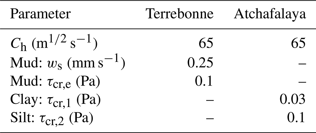
Table 1 summarizes the calibrated parameters for each model and the corresponding remote sensing data used, whereas Fig. 3 shows the chosen flight lines of the three instruments.
Table 1Calibrated parameters and relative remote sensing data used for each model.
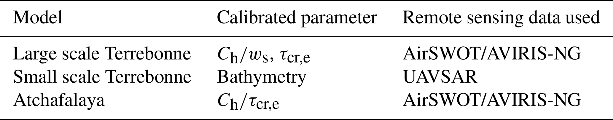
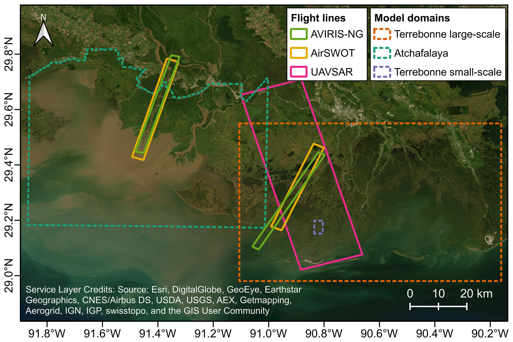
Figure 3Extension of the flight lines used in this study. The extension of the numerical models is also reported with thinner lines.
In all three models, the coupling between remote sensing images and the model allowed the parameters to be tuned to best match numerical outputs and the observations. Water levels and sediment concentration from the numerical models were extracted using the spatial extent of the chosen flight lines and overlapped to enable comparisons. The comparison was first performed visually, in order to identify evident discrepancies. Then, a pixel-by-pixel comparison was performed to better quantify model performance. For the Terrebonne large-scale model and the Atchafalaya model, because of the 90 m mesh resolution, both AirSWOT and AVIRIS-NG resolution was lowered by averaging values within a 90 m mesh element. The evaluation of the models was performed by computing the error as the difference between the measurement and the modeled values, with a positive error indicating underestimation. The RMSE was adopted as a global metric to compare the overall performance of each simulation. Parameter values providing the lowest RMSE were identified as the optimal ones.
In the large-scale Terrebonne model, a second calibration of the Chezy coefficient and sediment properties was performed using only in situ observations. Simulated water levels during the Spring campaign were compared with time series of 13 tidal gauges within the CRMS network (Fig. S3). The RMSE and Nash–Sutcliffe Model Efficiency (Allen et al., 2007) were used to evaluate model performance for the different friction coefficients. The validation with time series allowed the temporal coherence of the results that cannot be captured by remote sensing to be evaluated. The two calibrations were validated in the Fall campaign by comparing water levels. In the same model, a calibration of sediment parameters using in situ measurements was carried out. Measured TSS concentrations from Fichot et al. (2022) were compared with simulation results (see Fig. S5). Finally, the two calibrations were validated using in situ TSS data collected during the Fall campaign (Fichot et al., 2022). RMSE was used to compare model results.
To validate the topographic correction in the small-scale model, the original and calibrated topography were compared with Real-Time Kinematics elevation measurements collected during the Delta-X Spring 2021 campaign (Twilley and Rovai, 2022) and the site 421 elevation provided by the CRMS.
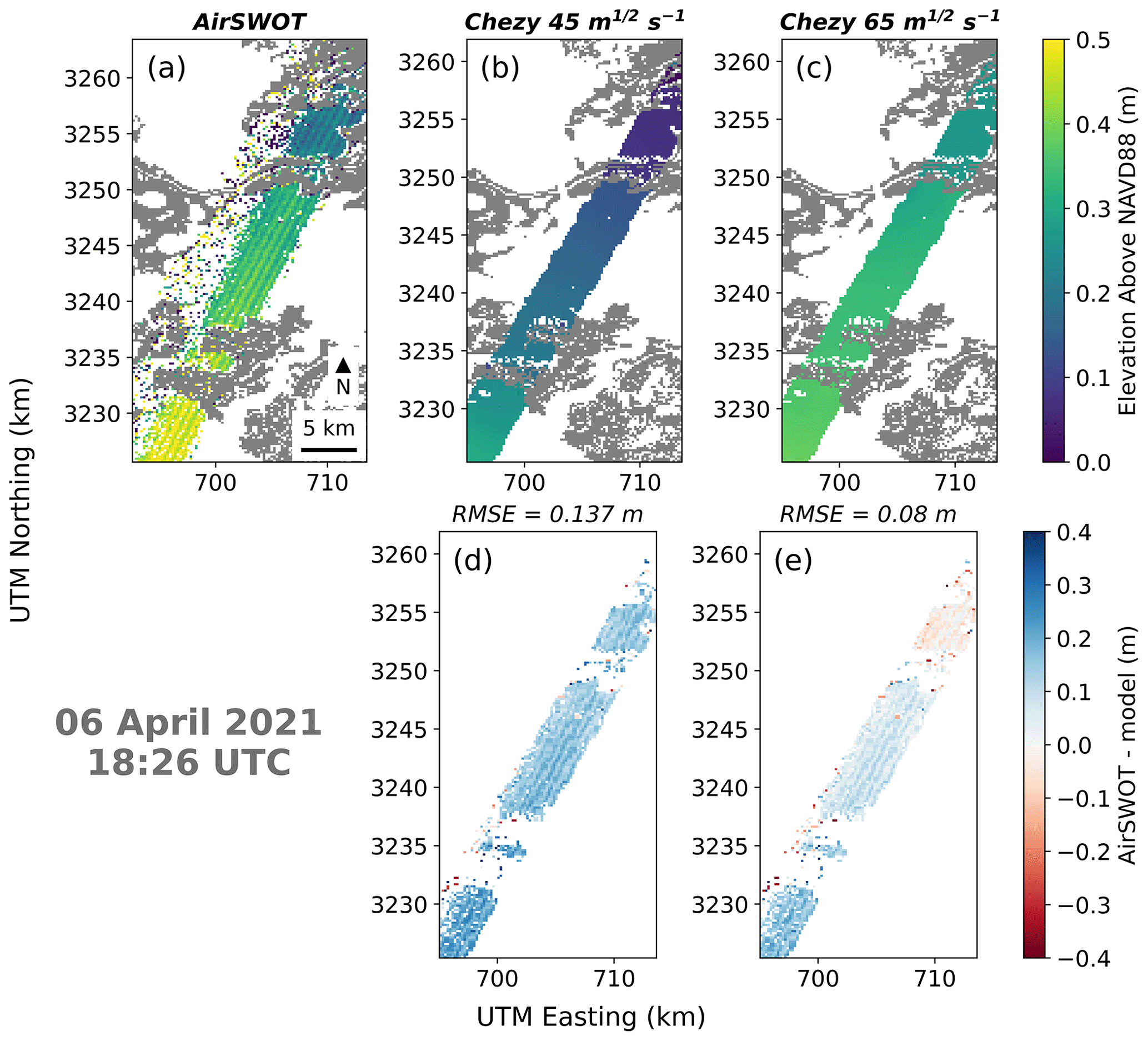
Figure 4Comparison between measured water levels by AirSWOT and modeled water levels within the large-scale Terrebonne model. From left to right AirSWOT elevation, modeled elevation with Ch=45 m s−1 and modeled elevation with Ch=65 m s−1 are presented. On the bottom row the difference between AirSWOT and the model results are displayed with the overall RMSE.
3.1 Coupling with AirSWOT
For the Terrebonne large-scale model, results of simulations with Chezy values of 65 and 45 m s−1 are shown for one acquisition (Fig. 4). The comparisons for four acquisitions of the same flight line at different times during the tidal cycle are reported in Fig. S2. The flight line has south-west to north-east direction. In the south, it crosses a channel with a 500–700 m cross-section and one of the major lakes in Terrebonne (Caillou Lake). In the north, it intersects a portion of other lakes and small channels. A Chezy coefficient of 65 m s−1 returns a better match with the AirSWOT observations except for the third acquisition on 6 April 2010 20:10 UTC (Fig. S2c); slightly better results were found for a Chezy coefficient of 45 m s−1. The model displays better agreement in the south section of the flight line, whereas the discrepancy between remote sensing data and model results tends to increase in the north section. The use of a friction coefficient of 65 m s−1 allows the water levels in the northern section of the flight line to be better represented.
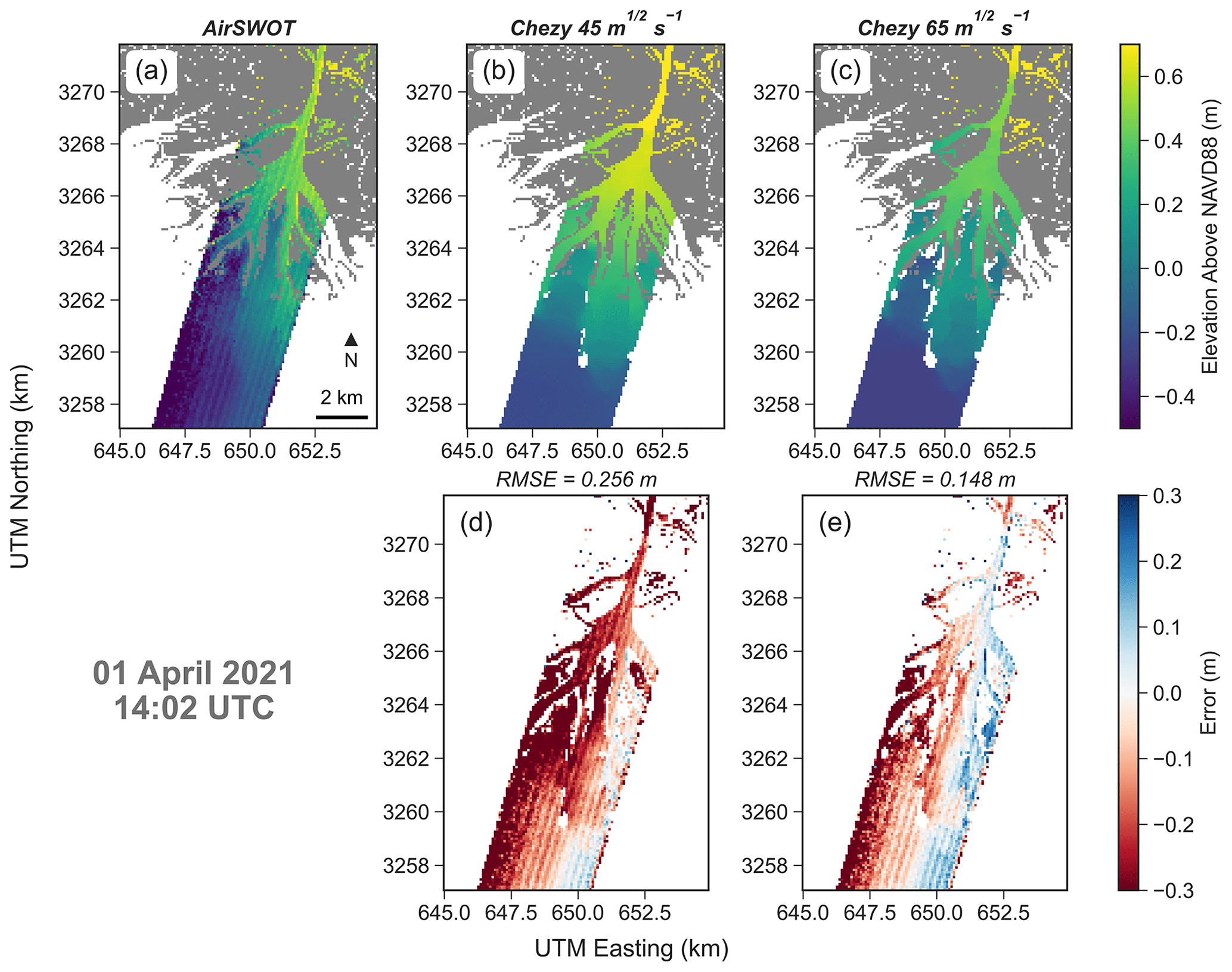
Figure 5Comparison between measured water levels by AirSWOT and modeled water levels in Atchafalaya Bay (with a focus on the Wax Lake Delta). From left to right, AirSWOT elevation, modeled elevation with Ch=45 m s−1 and modeled elevation with Ch=65 m s−1 are presented.
Figure S5a, b show the results of the calibration using time series of stationary gauges. The calibration shows similar results, with Ch=45 m s−1 providing the better RMSE. The validation of the friction coefficient during the Fall campaign (Fig. S5c, d) shows better performance for Ch=65 m s−1, with a RMSE of 0.047 m compared with the 0.066 m for the 45 m s−1 case.
The calibrated value of 65 m s−1 for the Chezy coefficient is comparable to Manning values for the area. If we consider an average modeled water depth of 1.34 m during the AirSWOT acquisitions and use the water depth as an approximation for hydraulic radius, a corresponding Manning coefficient (Limerinos, 1970) can be estimated. The equation yields n=0.02 m s−1 which is within the range of values suggested by the 1992 NLCD and LA-GAP classification for the open water class (Bunya et al., 2010).
Atchafalaya model results with Chezy values of 45 and 65 m s−1 (Fig. 5) are shown for the Wax Lake Delta. A Chezy coefficient of 65 m s−1 drastically improves model performance compared with the 45 m s−1 case, with a reduction of the RMSE from 25.6 to 14.3 cm. In particular, the reduction of bottom friction allows the model to better represent water elevations in the main channel, but especially in the vicinity of the distributary channels of the delta where the model with 45 m s−1 tends to overestimate water elevations. Furthermore, the 65 m s−1 simulation detects the west-to-east surface slope.
Table 2Parameters for the large-scale models calibrated with AirSWOT and AVIRIS-NG data.
3.2 Coupling with UAVSAR
Data of water-level changes measured during the 12 April 2021 UAVSAR flight were used to correct marsh topography. The campaign took place between t1=19:29 and t2=22:59 (UTC time). The data collected in this temporal window offer a synoptic view of water-level change across the marsh landscape during falling tides. As water-level change is computed as the difference between the measurements at t2 and t1, the negative values in Fig. 6a confirm that the waters on the marsh are receding. Results from the first run (Fig. 6b, d) highlight two critical areas. First, the model overestimates the water-level change in the southern area, indicating an error in the marsh elevation derived from LiDAR data. The opposite is occurring in the northern area, where waters are found to recede too slowly and consequently the water-level change is underestimated. Thus, the original topography (Fig. 6f) was modified with the described step-wise approach, and after four iterations the new topography (Fig. 6g) increased model performance (Fig. 6c), with RMSE decreasing from 4.9 to 3.9 cm. During each step, model performance increased and after four iterations, changes in topography and RMSE were negligible. On average, the total elevation change was −0.013 m, indicating the general need to lower the elevation. The topography modifications (Fig. 6h) reproduced water-level changes well (Fig. 6a), particularly in the critical areas previously highlighted.
Validation results are reported in Fig. S5. Overall, the correction based on UAVSAR decreases the elevation error from 18.94 to 9.78 cm. Despite the general improvement, for some specific points the correction increased the error. In particular, the bathymetry was strongly deepened at three locations.
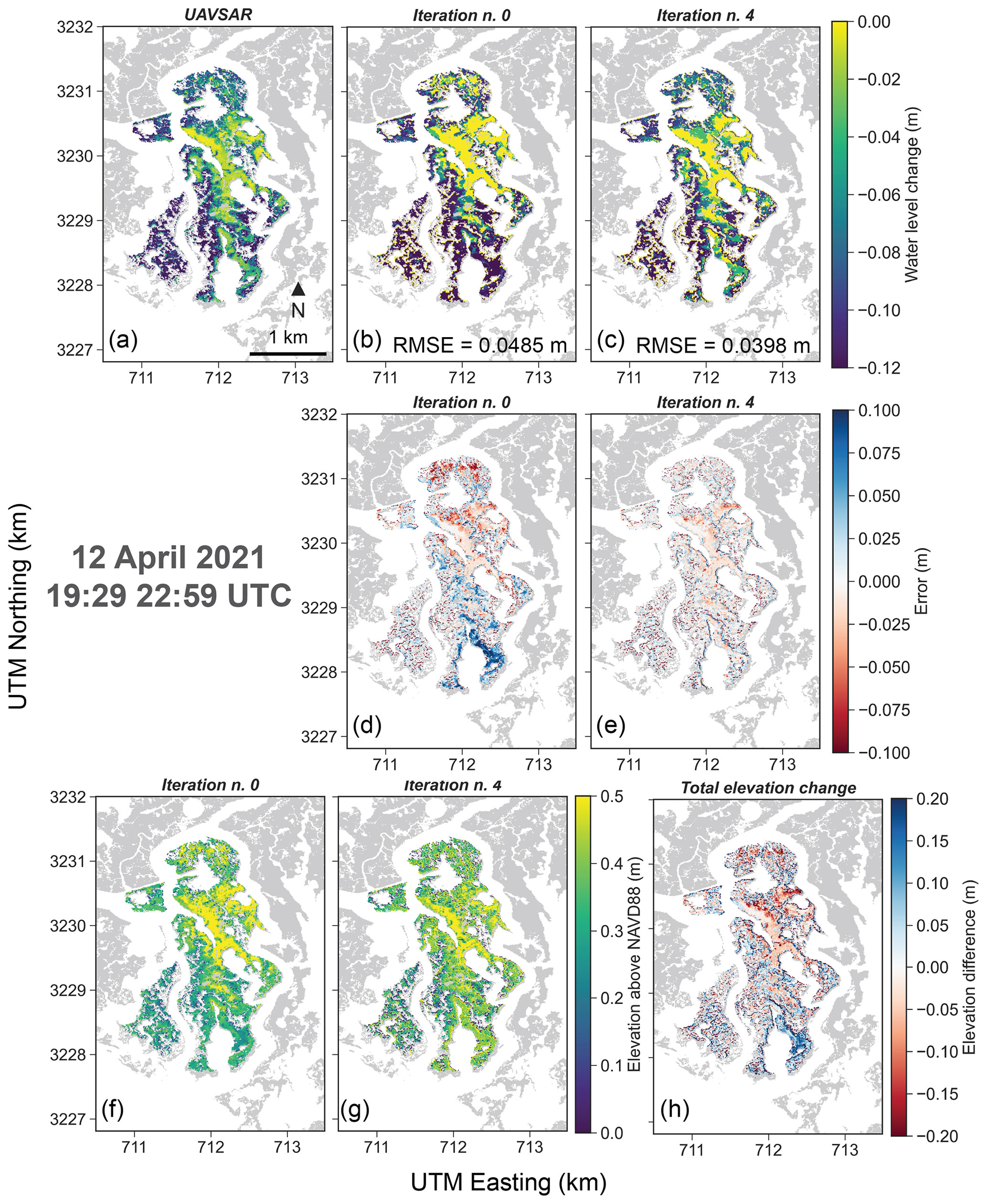
Figure 6Comparison between (a) water-level changes in vegetated areas measured by UAVSAR during the 12 April 2021 UAVSAR flight between 19:29 and 22:59 (UTC time), and water-level changes obtained via numerical modeling by using: (b) the initial marsh topography, and (c) the corrected topography after four iterations. Subplots (d) and (e) show the model error at the first and fourth iterations respectively. Comparison between (f) initial marsh topography and (g) marsh topography after four iterations of the correction method. Subplot (h) shows the total implemented changes in bed elevation.
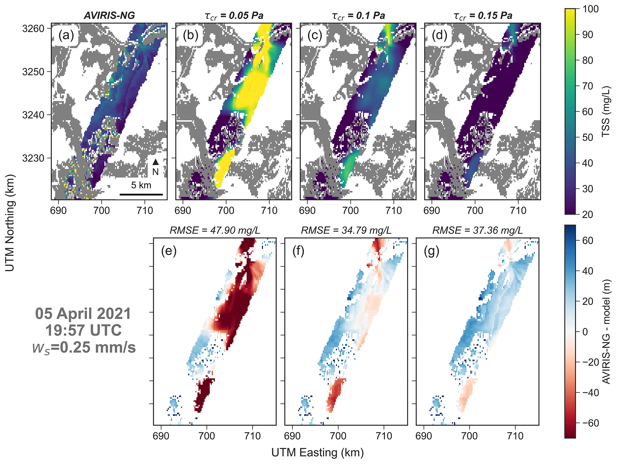
Figure 7Comparison between AVIRIS-NG and the modeled sediment concentration. The settling velocity is fixed at 0.25 mm s−1 and the critical shear stress is changed. The first map on the top row shows the sediment concentration derived from AVIRIS-NG, whereas the next three maps show the modeled sediment concentration for different critical shear stress. The bottom rows show the error between measurements and model. At the top of each error map the RMSE is indicated. The sediment concentration color bar is fixed between the minimum and maximum value of the measured sediment concentration, whereas the error color bar is fixed between the overall minimum and maximum computed error.
3.3 Coupling with AVIRIS-NG
For the Terrebonne model, the AVIRIS-NG acquisition taken on 5 April 2021 at 19:57:00 GMT (Figs. 7 and 8) is considered. The flight line crosses the open coast and Caillou Lake from south-west to north-east. Results show that sediment concentrations tend to decrease as the critical shear stress increases (Fig. 7). For τcr,e=0.05 Pa, the models tend to overestimate the sediment concentrations. The best agreement (lowest RMSE) occurs at value 0.1 Pa. For τcr,e=0.15 Pa, the error increases again with an underestimation of sediment concentration. Figure 8 shows the effect of settling velocity. When ws=0.1 mm s−1 the sediment concentration is grossly overestimated. With higher values of settling velocity, the comparison improves, until it reaches the lowest RMSE of 34.79 mg L−1 for ws=0.25 mm s−1. For higher values, the agreement declines, and the model tends to underestimate sediment concentrations. The flight line also crosses a meander of a large channel (center-right position). Here, the model tends to always overestimate sediment concentration and the error decreases as critical shear stress and settling velocity increase. Overall, the model performs better in the open sections of the flight line, whereas at the extremities, performance declines. The combination that provides the best comparison with measurements is a critical shear stress of 0.1 Pa and a sediment settling velocity of 0.25 mm s−1.
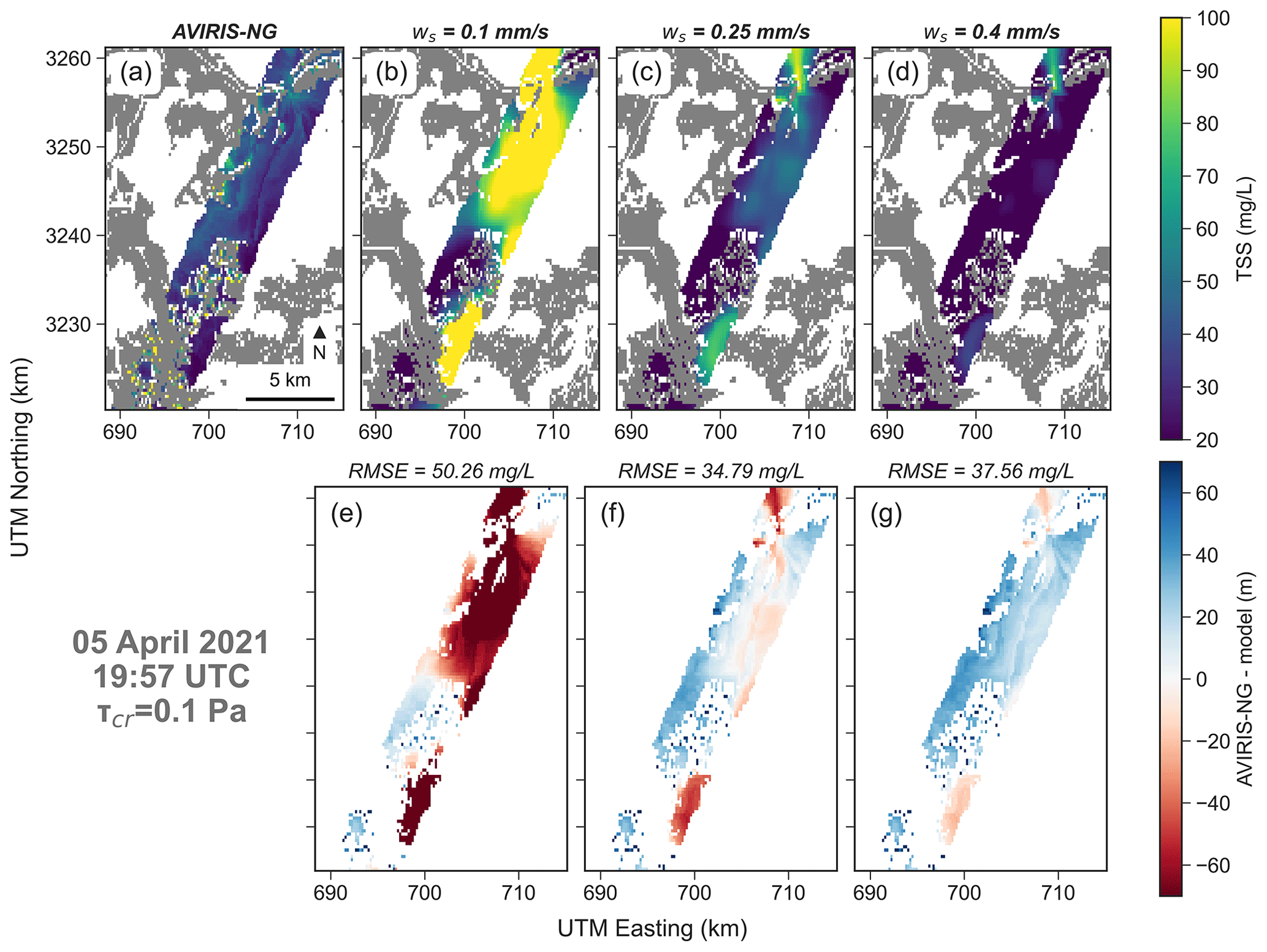
Figure 8Comparison between AVIRIS-NG and the modeled sediment concentration. The critical shear stress is fixed at 0.1 Pa and the settling velocity is changed. The first map on the top row shows the sediment concentration derived from AVIRIS-NG, whereas the next three maps show the modeled sediment concentration for different settling velocities. The bottom rows show the error between measurements and model. At the top of each error map the RMSE is indicated.
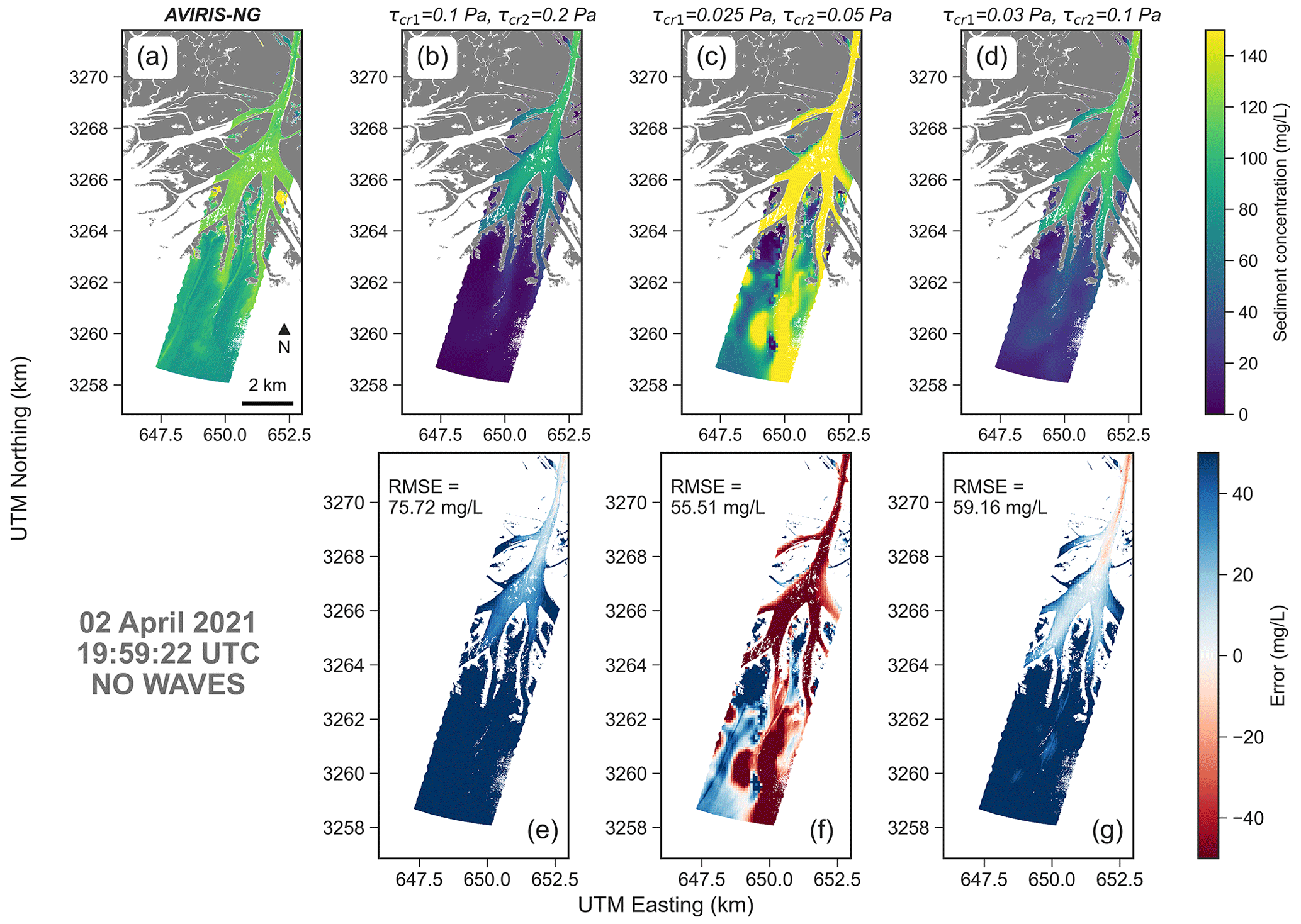
Figure 9Comparison between AVIRIS-NG and the modeled sediment concentration in the Wax Lake Delta without waves. Scenarios show model results with different critical shear stresses for clay (τcr,1) and silt (τcr,2).
Settling velocity calibrated using only in situ measurements was found to be 0.325 mm s−1, different from the value obtained from the remote sensing images (Fig. S7). The optimal critical shear stress was identical (0.1 Pa). This combination provided the lowest RMSE of 25.26 mg L−1. During the Fall campaign, when the two calibrations were compared, the calibration performed using AVIRIS-NG provided better agreement with in situ measurements than the calibration with in situ measurements only (Fig. S8).
For the Wax Lake model, the acquisition taken on 2 April 2021 at 19:59:22 GMT is considered (Figs. 9 and 10). A lower critical shear stress generates higher sediment concentrations, consistent with the Terrebonne model. In particular, the best match is obtained for τcr,1=0.03 Pa (clay) and τcr,2=0.1 Pa (silt), with a RMSE of 35.88 mg L−1 (Fig. 10g). In this case, results improve when waves are included in the simulation. This is evident in the shallow areas near the delta, suggesting that wave resuspension must be included despite the system being river dominated. In the other two cases the model tends to underestimate (τcr,1=0.1 Pa and τcr,2=0.2 Pa) and overestimate (τcr,1=0.025 Pa and τcr,2=0.05 Pa) sediment concentrations.
The combination of AirSWOT, UAVSAR, and AVIRIS-NG enables calibration and evaluation of different parameters of the numerical model at spatial scales that in situ point measurements cannot capture. AirSWOT and UAVSAR data can greatly improve hydrodynamic models. In particular, their combination enables evaluation of the goodness of computed water fluxes in bays, tidal channels, and on the marsh platform. AVIRIS-NG-derived sediment concentration enables evaluation of the models’ ability to reproduce sediment resuspension and transport.
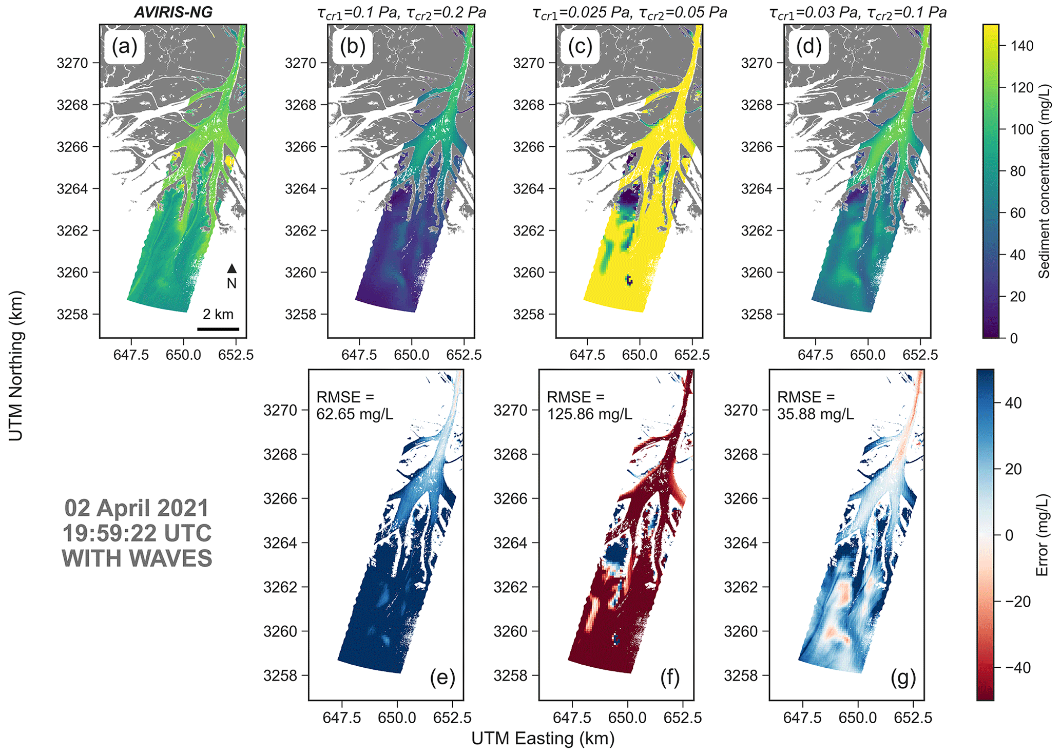
Figure 10Comparison between AVIRIS-NG and the modeled sediment concentrations in the Wax Lake Delta with the effect of waves. Scenarios show model results with different critical shear stresses for clay (τcr,1) and silt (τcr,2).
4.1 AirSWOT
The comparison between hydrodynamic models and remote sensing imagery shows that the model can reproduce the water levels in the southern half of the flight line. The results are comparable with other modeling studies at the same location and in similar intertidal areas along the US Atlantic coast. For instance, Mariotti et al. (2010) and Palazzoli et al. (2020) developed models for the shallow coastal bays of the Virginia Coastal Reserve and obtained RMSE of 0.07–0.11 and 0.26 m respectively. In Louisiana, Freeman et al. (2015) modeled the impact of Hurricane Rita in one of the major coastal lakes in Terrebonne Bay, obtaining an RMSE of 0.1 m, whereas Ou et al. (2020) developed a salinity model in Barataria Bay and found an RMSE of between 0.05 and 0.14 m for water levels.
In the northern part of the large-scale Terrebonne Bay model, water levels tend to be regularly underestimated especially in the areas further north not shown in Figs. 4 and S2. AirSWOT data highlight zones where model performance needs to be addressed. Errors can be related to uncalibrated bed friction coefficients. In some cases, the model underestimates the water levels by 0.3 m, which represents a significant error because the tidal range is around 0.4 m (Georgiou et al., 2005). The issue could be addressed by increasing the Chezy coefficient. However, for such a large discrepancy between water levels, this would likely yield large and unrealistic values. In this case, there is a hydraulic connectivity problem, namely, the model is not able to fully propagate the tides in the northern areas. The limitation lies in the coarse resolution of the mesh (90×90 m), which cannot capture the intricate network of narrow channels that connects the upper and lower portions of the domain. One way to address the issue is to carve and enlarge the channels until there is a satisfactory match between model and remote sensing data (Zhang et al., 2022b). It has to be noted that the AirSWOT flight lines present a large error at the edges (blue areas in Fig. 5a) because the incident angle of the outer swath mode is within 4 and 25∘ (Denbina et al., 2019).
In the Atchafalaya model, similar errors are observed. Water elevations in areas located in the wetlands north of the Wax Lake Delta tend to be overestimated. The reason can be similarly explained as in the Terrebonne model: the low spatial resolution does not correctly represent the narrow channels. However, the model replicated the water levels in the delta well owing to the wide cross section of the main distributaries (between 200–500 m).
It is also worth noting that the correct boundary conditions must be imposed before calibration with the remote sensing imagery. The boundary condition in the large-scale model is the water-level signal from the Gulf of Mexico, which was indirectly inferred from a USGS water-level gauge located along the coast. Similarly, the boundary conditions at the ocean in the Atchafalaya model was indirectly inferred from a NOAA station located off-shore. Although it was not used here for this purpose, AirSWOT can also be used to verify discharge boundary conditions in models where a riverine discharge is imposed (Zhang et al., 2022a).
The validation of the water levels across the domain using in situ measurements further confirms the goodness of the calibrated friction coefficient using AirSWOT (Fig. S4). Despite the lack of spatial information, time series can fill the temporal gap of remote sensing imagery. A combination of both types of data is a powerful tool for a holistic calibration and validation of numerical models.
4.2 UAVSAR
The difference between observed and modeled changes in water level over a fixed time was employed to correct marsh topography. If such a difference is large, more flow conveyance is needed to increase water-level changes, and vice versa. This can be done by modifying the marsh elevation or the drag coefficient, or both. As suggested by Zhang et al. (2022a), friction plays a marginal role in affecting water levels on marsh platforms. They run a sensitivity analysis with a wide range of friction values and found little effect on model performance. The calibration of topography inherently contains information on friction, which can lead to its small effect on the computed flow field. Applying the same iterative method to friction only, without modifying marsh elevation, would lead to unrealistically large spatial variations of the friction coefficient. Therefore, it was decided to only change marsh elevation to match modeled water-level variations with those derived via UAVSAR.
The ability of a model to correctly simulate water fluxes is tightly dependent on having accurate and precise marsh topography. This is especially true in coastal Louisiana, where tidal ranges are small. Here, even a small topographic change can lead to notable variations in the flooding period (Donatelli et al., 2023a). Bathymetric data from LiDAR may present a positive bias in vegetated areas owing to the inability of laser pulses to penetrate dense thick vegetation (Rosso et al., 2006). Furthermore, such bias is spatially variable and depends on vegetation characteristics (Medeiros et al., 2015). UAVSAR data can fill this gap. A simple comparison between model results and remote sensing data allowed precise identification of critical parts of the domain and improvement of water fluxes on the marsh. The adjustment of the marsh elevation could also be carried out by adding or subtracting a constant value. However, UAVSAR allows the elevation at each point to be adjusted based on local hydrodynamics, unraveling the effect of micro-topography on water flow.
Starting from the initial topography, at each iteration the RMSE decreases until the minimum value of 3.9 cm is reached. The error in the subsequent iterations increases as the procedure begins to over-correct the topography and introduces errors that result in worse performance. It is important to highlight that this methodology is empirical and might have some theoretical issues. For instance, by modifying the bed elevation at some location of a marsh, water levels will change in surrounding areas. Thus, this iterative procedure may introduce errors in areas where the topography is correct. The methodology also depends on how well the model can solve the tidal channels. This effect can be noted for the three points previously mentioned where the marsh was deepened. In this case, the points are located in proximity to a narrow channel with a 1.5–2 m cross section. The 10 m resolution of the model represents a limitation because features such as channels and levees that are smaller than 10 m cannot be captured by the mesh. In this example, the UAVSAR flight line captured the flow during falling tide, and during this phase, areas of the marsh close to the channels drained faster than internal ones. As the model does not capture these channels, the method tries to compensate by lowering the marsh to increase water fluxes even if the elevation is correct.
Another drawback of this approach is that the bathymetric correction is based on water-level changes detected by UAVSAR during a very short period between 19:29 and 22:59 UTC time on 12 April 2021. Such changes are only representative of the temporal window in which the UAVSAR campaign took place. Although the solution was improved, the choice of a different acquisition might yield a different final marsh topography.
4.3 AVIRIS-NG
The use of AVIRIS-NG is possible after the calibration and validation of the hydrodynamic model, as sediment concentration depends on both the properties of sediment particles and hydrodynamic forcing. For the large-scale Terrebonne model, the calibrated critical shear stress and settling velocity are comparable with those of previous studies in Terrebonne Bay (e.g., Liu et al., 2018). Along the flight line, the lower portion of the model in the coastal waters of the Gulf of Mexico and the Caillou Lake portion in the middle provide the best match with the imagery, despite the fact that the modeled concentration tends to be more homogeneous. Overall, considering the relatively low RMSE compared with the full range of sediment concentration, it is concluded that the model can capture resuspension of bottom sediments. The model is also able to reproduce the sediment plume entering Caillou Lake, although it overestimates the concentration.
A calibration using only measurements in the field presents limitations. The optimal set of parameters is ws=0.325 mm s−1, τcr,e=0.1 Pa (Fig. S6h), which differs from the best set found using AVIRIS-NG (ws=0.25 mm s−1, τcr,e=0.1 Pa). Interestingly, the validation shows that, despite the model tending to underestimate concentrations in both cases, the calibration with AVIRIS-NG provides the lowest RMSE (Fig. S8). AVIRIS-NG also provides the possibility of comparing the results with spatially distributed data, allowing a more complete evaluation of model performance. Point measurements could also not cover the full range of concentration and lead to calibrated parameters not representative of the entire area. Especially in coastal areas, cohesive sediment properties are highly affected by flocculation. Fine sediment aggregate to form flocs, for which both settling velocity and bed shear strength are highly uncertain and difficult to predict.
In the Terrebonne large-scale model there are also discrepancies in the northern areas and within the channel meander in the south-eastern portion of the flight line, where the model tends to overestimate sediment concentrations. These errors might be related to bathymetric modification of the mesh. To allow a correct tidal propagation, channels were deepened and enlarged, which might have generated flow velocities different from real ones. Errors can also be attributable to model assumptions that are inherent to the developed model. Although Delft3D has 3D capabilities, a vertically averaged 2D model was chosen to avoid high computational costs and potential numerical instability of 3D grids when wetting and drying tidal flats and salt marshes are included. Moreover, 3D models do not provide a substantial improvement of predictability in water levels with respect to 2D models (Bates, 2022).
It is fundamental to consider that AVIRIS-NG measures TSS concentration at the water surface. As the models are depth averaged, a well-mixed column is implicitly assumed, which is a condition that may not always be true. Along rivers, sediment concentration has been typically observed to increase from the surface to the bed (Lamb et al., 2020). Usually, the coarser fraction occupies the lower layers in the water column, whereas finer fractions are resuspended to the surface. Hence, because AVIRIS-NG can only characterize the water surface, TSS maps might not be representative of total transport, which represents a limitation for the calibration of sediment properties. The well-mixed conditions may not also be present in sheltered areas. In these locations, vertical heterogeneity is promoted by density gradients and low-energy conditions during low wind-speed conditions (Kjerfve and Magill, 1989). The lack of sediment heterogeneity could also be a reason for the concentration underestimation on the western side of the flight line in the large-scale Terrebonne model. Here, calibrated simulations tend to be 30 mg L−1 lower than with AVIRIS-NG data. It is possible that in those areas only the finest fractions (not included in the current granulometry) are entrained in the water column. Another possible source of error is the absence of secondary flows and 3D flow structures that might arise at the boundary between channels and the marsh platform (Proust and Nikora, 2020).
The AVIRIS-NG data suggest further evaluations. The comparison between the wave and no-wave cases (Figs. 9 and 10) shows that the inclusion of the wave-induced resuspension is fundamental to better capturing SSC in the deltaic areas. This result is consistent with previous research that highlighted the important role of waves in the development of river deltas and the redistribution of sediment along the coastal inner shelf (Shi et al., 1997; Walker and Hammack, 2000; Corbett et al., 2007; Carniello et al., 2014). As a final note, it is worth mentioning that maps of TSS from AVIRIS-NG can also be leveraged independently from the numerical models. For instance, TSS maps in the Wax Lake Delta reveal distinctive patterns called streaklines (Kundu et al., 2015) (see Fig. 2c), that can be used to derive deposition and erosion patterns and flow velocity without the support of numerical models (Salter et al., 2022; Donatelli et al., 2023b).
This study shows the potential of calibrating numerical models using remote sensing imagery instead of traditional sparse field data. Images from two SAR sensors and one spectrometer sensor flown during the NASA Delta-X airborne mission were utilized for the calibration. UAVSAR measured water-level change on the marsh platform, whereas sediment transport parameters AirSWOT derived water elevations in bays, lakes, channels, and AVIRIS-NG measured sediment concentrations.
AirSWOT was used to calibrate the bottom friction coefficient in Terrebonne and Atchafalaya Basins, UAVSAR data to correct bathymetric errors and improve wetland flooding, and TSS maps derived from AVIRIS-NG allowed the sediment transport parameters to be calibrated. The use of spatially extended remote sensing imagery enabled areas where models performed better to be quickly evaluated and provided calibrated parameters that are consistent with previous literature values. Remote sensing data yield spatial information that point observations cannot capture. In the case of highly uncertain parameters, a calibration based entirely on fixed location measurements can lead to incorrect values, whereas imagery from remote sensing can provide a more spatially coherent dataset. At the same time, some limitations and considerations need to be accounted for when coupling imagery with a numerical model.
Finally, the use of water-level time series at different locations for the validation informed the temporal performance of the models. Given the limited number of flyovers, temporal data allow the accuracy of the calibration to be verified and test whether the model reproduces coherent water elevations over a wider time window in specific points of the domain.
The array of available remote sensing data will grow in the near future. This study showed that a new generation of numerical models can be developed by leveraging the spatial information provided by remote sensors.
All Delta-X products and data used in this study are deposited at the correspondent ORNL-DAAC repository (https://daac.ornl.gov/daacdata/deltax/ (last access: 20 October 2023). Water-level data from the Coastwide Reference Monitoring System (CRMS) used for the large-scale Terrebonne model validation and small-scale Terrebonne model boundary conditions are publicly available via the CPRA website (https://cims.coastal.louisiana.gov/monitoring-data/, last access: 20 October 2023, CPRA, 2023). Water-level data from the USGS station 073813498 used as boundary conditions in the large-scale Terrebonne model are available via the USGS website (https://doi.org/10.5066/F7P55KJN, U.S. Geological Survey, 2016). Water discharge and sediment concentration data for the Atchafalaya model from the USGS stations 07381590 and 07381600 are available via the USGS website (https://doi.org/10.5066/F7P55KJN, U.S. Geological Survey, 2016) and (https://doi.org/10.5066/F7P55KJN, U.S. Geological Survey, 2016) respectively. Water-level data from the Eugene Island NOAA station used as oceanic boundary condition in the Atchafalaya model are available via the NOAA website (https://doi.org/10.25921/dt9g-2p60, CO-OPS, 2018.).
The supplement related to this article is available online at: https://doi.org/10.5194/bg-21-241-2024-supplement.
LC, CD, XZ performed the simulations and interpreted the results. SF supervised the project. LC wrote the manuscript with contributions from all co-authors.
The contact author has declared that none of the authors has any competing interests.
Publisher’s note: Copernicus Publications remains neutral with regard to jurisdictional claims made in the text, published maps, institutional affiliations, or any other geographical representation in this paper. While Copernicus Publications makes every effort to include appropriate place names, the final responsibility lies with the authors.
This article is part of the special issue “Monitoring coastal wetlands and the seashore with a multi-sensor approach”. It is not associated with a conference.
This research was funded by the NASA Delta-X project (the Science Mission Directorate's Earth Science Division through the Earth Venture Suborbital-3 Program NNH17ZDA001N-EVS3). Luca Cortese was supported by the Future Investigators in NASA Earth and Space Science and Technology (FINNEST) award number 80NSSC21K1612. Sergio Fagherazzi was also supported by the Virginia Coast Reserve Long-Term Ecological Research Program (National Science Foundation DEB-1832221) and the Plum Island Ecosystems Long-Term Ecological Research Program (National Science Foundation OCE-2224608). This work was carried out in part at the Jet Propulsion Laboratory, California Institute of Technology, under a contract with the National Aeronautics and Space Administration. We are grateful to Michael P. Lamb, Paola Passalacqua, Robert Twilley, and all Delta-X team members that contributed to the conceptualization of the Delta-X mission and the data included in this study.
This research has been supported by the National Aeronautics and Space Administration (grant nos. NNH17ZDA001N-EVS3 and 80NSSC21K1612), the Directorate for Biological Sciences (grant no. 1832221), and the Directorate for Geosciences (grant no. 2224608).
This paper was edited by Beatrice Maria Sole Giambastiani and reviewed by three anonymous referees.
Allen, J., Somerfield, P., and Gilbert, F.: Quantifying uncertainty in high-resolution coupled hydrodynamic-ecosystem models, J. Mar. Syst., 64, 3–14, https://doi.org/10.1016/j.jmarsys.2006.02.010, 2007. a
Allison, M. A., Kineke, G. C., Gordon, E. S., and Goni, M. A.: Development and reworking of a seasonal flood deposit on the inner continental shelf off the Atchafalaya River, Cont. Shelf Res., 20, 2267–2294, https://doi.org/10.1016/S0278-4343(00)00070-4, 2000. a
Balogun, A.-L., Yekeen, S. T., Pradhan, B., and Althuwaynee, O. F.: Spatio-temporal analysis of oil spill impact and recovery pattern of coastal vegetation and wetland using multispectral satellite landsat 8-OLI imagery and machine learning models, Remote Sens., 12, 1225, https://doi.org/10.3390/rs12071225, 2020. a
Bates, P. D.: Flood inundation prediction, Annu. Rev. Fluid Mech., 54, 287–315, https://doi.org/10.1146/annurev-fluid-030121-113138, 2022. a
Bevington, A. E. and Twilley, R. R.: Island edge morphodynamics along a chronosequence in a prograding deltaic floodplain wetland, J. Coast. Res., 34, 806–817, https://doi.org/10.2112/JCOASTRES-D-17-00074.1, 2018. a
Booij, N. and Holthuijsen, L. H.: Propagation of ocean waves in discrete spectral wave models, J. Comput. Phys., 68, 307–326, https://doi.org/10.1016/0021-9991(87)90060-X, 1987. a
Bue, B. D., Thompson, D. R., Eastwood, M., Green, R. O., Gao, B.-C., Keymeulen, D., Sarture, C. M., Mazer, A. S., and Luong, H. H.: Real-time atmospheric correction of AVIRIS-NG imagery, IEEE T. Geosci. Remote, 53, 6419–6428, https://doi.org/10.1109/TGRS.2015.2439215, 2015. a
Bunya, S., Dietrich, J. C., Westerink, J. J., Ebersole, B. A., Smith, J. M., Atkinson, J. H., Jensen, R., Resio, D. T., Luettich, R. A., Dawson, C., Cardone, V. J., Cox, A. T., Powell, M. D., Westerink, H. J., and Roberts, H. J.: A high-resolution coupled riverine flow, tide, wind, wind wave, and storm surge model for southern Louisiana and Mississippi, Part I: Model development and validation, Mon. Weather Rev., 138, 345–377, https://doi.org/10.1175/2009MWR2906.1, 2010. a, b
Cahoon, D. R., Hensel, P. F., Spencer, T., Reed, D. J., McKee, K. L., and Saintilan, N.: Coastal Wetland Vulnerability to Relative Sea-Level Rise: Wetland Elevation Trends and Process Controls, edited by: Verhoeven, J. T. A., Beltman, B., Bobbink, R., and Whigham, D. F., Wetlands and Natural Resource Management, Ecological Studies, 190, 271–292, Springer, Berlin, Heidelberg, https://doi.org/10.1007/978-3-540-33187-2_12, 2006. a
Cardoso, G. F., Souza, C., and Souza-Filho, P. W. M.: Using spectral analysis of Landsat-5 TM images to map coastal wetlands in the Amazon River mouth, Brazil, Wetlands Ecol. Manage., 22, 79–92, https://doi.org/10.1007/s11273-013-9324-4, 2014. a
Carniello, L., Silvestri, S., Marani, M., D'Alpaos, A., Volpe, V., and Defina, A.: Sediment dynamics in shallow tidal basins: In situ observations, satellite retrievals, and numerical modeling in the Venice Lagoon, J. Geophys. Res.-Ea., 119, 802–815, https://doi.org/10.1002/2013JF003015, 2014. a
Castagno, K. A., Jiménez-Robles, A. M., Donnelly, J. P., Wiberg, P. L., Fenster, M. S., and Fagherazzi, S.: Intense storms increase the stability of tidal bays, Geophys. Res. Lett., 45, 5491–5500, https://doi.org/10.1029/2018GL078208, 2018. a
Center for Operational Oceanographic Products and Services (CO-OPS): CO-OPS Water Level Data from the Coastal Tide Gauge and Great Lake Water Level Network of the United States and US Territories, NOAA National Centers for Environmental Information, [data set], https://doi.org/10.25921/dt9g-2p60, 2018. a
Chen, C., Ma, Y., Ren, G., and Wang, J.: Aboveground biomass of salt-marsh vegetation in coastal wetlands: Sample expansion of in situ hyperspectral and Sentinel-2 data using a generative adversarial network, Remote Sens. Environ., 270, 112885, https://doi.org/10.1016/j.rse.2021.112885, 2022. a
Coastal Protection and Restoration Authority (CPRA) of Louisiana: Coastwide Reference Monitoring System-Wetlands Monitoring Data, Retrieved from Coastal Information Management System (CIMS) database, [data set], http://cims.coastal.louisiana.gov (last access: 20 October 2023), 2023. a
Corbett, D. R., Dail, M., and McKee, B.: High-frequency time-series of the dynamic sedimentation processes on the western shelf of the Mississippi River Delta, Cont. Shelf Res., 27, 1600–1615, https://doi.org/10.1016/j.csr.2007.01.025, 2007. a
Cortese, L. and Fagherazzi, S.: Fetch and distance from the bay control accretion and erosion patterns in Terrebonne marshes (Louisiana, USA), Earth Surf. Proc. Land., 47, 1455–1465, https://doi.org/10.1002/esp.5327, 2022. a
Couvillion, B. R., Beck, H., Schoolmaster, D., and Fischer, M.: Land area change in coastal Louisiana (1932 to 2016), Tech. Rep., US Geological Survey, https://doi.org/10.3133/sim3381, 2017. a, b, c
Defne, Z. and Ganju, N. K.: Quantifying the residence time and flushing characteristics of a shallow, back-barrier estuary: Application of hydrodynamic and particle tracking models, Estuar. Coast., 38, 1719–1734, https://doi.org/10.1007/s12237-014-9885-3, 2015. a
Denbina, M., Simard, M., Rodriguez, E., Wu, X., Chen, A., and Pavelsky, T.: Mapping water surface elevation and slope in the Mississippi river delta using the AirSWOT Ka-Band interferometric synthetic aperture radar, Remote Sens., 11, 2739, https://doi.org/10.3390/rs11232739, 2019. a, b
Denbina, M., Simard, M., Pavelsky, T., Christensen, A., Liu, K., and Lyon, C.: Pre-Delta-X: Channel Bathymetry of the Atchafalaya Basin, LA, USA, 2016, ORNL DAAC, [data set], https://doi.org/10.3334/ORNLDAAC/1807, 2020. a, b
Denbina, M., Simard, M., and Rodriguez, E.: Delta-X: AirSWOT L2 Geocoded Water Surface Elevation, MRD, Louisiana, 2021, Version 2, ORNL DAAC, Oak Ridge, Tennessee, USA, [data set], https://doi.org/10.3334/ORNLDAAC/2128, 2022. a
Dietrich J. C., Westerink, J. J. , Kennedy, A. B., Smith, J. M., Jensen, R. E., Zijlema, M., Holthuijsen, L. H., Dawson, C., Luettich, R. A., Powell, M. D., Cardone, V. J., Cox, A. T., Stone, G. W., Pourtaheri, H., Hope, M. E., Tanaka, S., Westerink, L. G., Westerink, H. J., and Cobell, Z.: Hurricane Gustav (2008) waves and storm surge: hindcast, synoptic analysis, and validation in Southern Louisiana, Mon. Weather Rev., 139, 2488–2522, https://doi.org/10.1175/2011MWR3611.1, 2011. a
Donatelli, C., Passalacqua, P., Jensen, D., Jones, C., Oliver-Cabrera, T., and Fagherazzi, S.: Spatial variability in salt marsh drainage controlled by small scale topography, J. Geophys. Res.-Ea., 128, 11, https://doi.org/10.1029/2023JF007219, 2023a. a
Donatelli, C., Passalacqua, P., Wright, K., Salter, G., Lamb, M. P., Jensen, D., and Fagherazzi, S.: Quantifying flow velocities in river deltas via remotely sensed suspended sediment concentration, Geophys. Res. Lett., 50, e2022GL101392, https://doi.org/10.1029/2022GL101392, 2023b. a
Dorji, P. and Fearns, P.: A quantitative comparison of total suspended sediment algorithms: A case study of the last decade for MODIS and landsat-based sensors, Remote Sens., 8, 810, https://doi.org/10.3390/rs8100810, 2016. a
Edmonds, D. A. and Slingerland, R. L.: Significant effect of sediment cohesion on delta morphology, Nat. Geosci., 3, 105–109, https://doi.org/10.1038/ngeo730, 2010. a
Fagherazzi, S., Mariotti, G., Leonardi, N., Canestrelli, A., Nardin, W., and Kearney, W. S.: Salt marsh dynamics in a period of accelerated sea level rise, J. Geophys. Res.-Earth, 125, e2019JF005200, https://doi.org/10.1029/2019JF005200, 2020. a, b
Farber, S.: The value of coastal wetlands for protection of property against hurricane wind damage, J. Environ. Econ. Manage., 14, 143–151, https://doi.org/10.1016/0095-0696(87)90012-X, 1987. a
Fichot, C. and Harringmeyer, J.: Delta-X: In Situ Water Surface Reflectance across MRD, LA, USA, 2021, Version 2, ORNL DAAC, [data set], https://doi.org/10.3334/ORNLDAAC/2076, 2021. a
Fichot, C. and Harringmeyer, J.: Delta-X: AVIRIS-NG L3-derived Water Quality, TSS, and Turbidity, MRD, LA 2021, V2, ORNL DAAC, [data set], https://doi.org/10.3334/ORNLDAAC/2112, 2022. a, b
Fichot, C., Ghosh, N., Harringmeyer, J., and Weiser, M.: Delta-X: Total Suspended Solids Concentration across MRD, LA, USA, 2021, Version 2, ORNL DAAC, [data set], https://doi.org/10.3334/ORNLDAAC/2075, 2022. a, b
Fichot, C. G., Downing, B. D., Bergamaschi, B. A., Windham-Myers, L., Marvin-DiPasquale, M., Thompson, D. R., and Gierach, M. M.: High-resolution remote sensing of water quality in the San Francisco Bay–Delta Estuary, Environ. Sci. Technol., 50, 573–583, https://doi.org/10.1021/acs.est.5b03518, 2016. a
Freeman, A. M., Jose, F., Roberts, H. H., and Stone, G. W.: Storm induced hydrodynamics and sediment transport in a coastal Louisiana lake, Estuar. Coast. Shelf Sci., 161, 65–75, https://doi.org/10.1016/j.ecss.2015.04.011, 2015. a
Galbraith, H., Jones, R., Park, R., Clough, J., Herrod-Julius, S., Harrington, B., and Page, G.: Global climate change and sea level rise: potential losses of intertidal habitat for shorebirds, Waterbirds, 25, 173–183, https://doi.org/10.1675/1524-4695(2002)025[0173:GCCASL]2.0.CO;2, 2002. a
Ganju, N. K. and Schoellhamer, D. H.: Decadal-timescale estuarine geomorphic change under future scenarios of climate and sediment supply, Estuar. Coast., 33, 15–29, https://doi.org/10.1007/s12237-009-9244-y, 2010. a
Ganju, N. K., Defne, Z., Kirwan, M. L., Fagherazzi, S., D'Alpaos, A., and Carniello, L.: Spatially integrative metrics reveal hidden vulnerability of microtidal salt marshes, Nat. Commun., 8, 14156, https://doi.org/10.1038/ncomms14156, 2017. a
Gao, B.-C., Heidebrecht, K. B., and Goetz, A. F.: Derivation of scaled surface reflectances from AVIRIS data, Remote Sens. Environ., 44, 165–178, https://doi.org/10.1016/0034-4257(93)90014-O, 1993. a
Georgiou, I. Y., FitzGerald, D. M., and Stone, G. W.: The impact of physical processes along the Louisiana coast, J. Coast. Res., 72–89, http://www.jstor.org/stable/25737050 (last access: 20 October 2023), 2005. a
Ghosh, S., Mishra, D. R., and Gitelson, A. A.: Long-term monitoring of biophysical characteristics of tidal wetlands in the northern Gulf of Mexico – A methodological approach using MODIS, Remote Sens. Environ., 173, 39–58, https://doi.org/10.1016/j.rse.2015.11.015, 2016. a
Goldstein, R. M. and Zebker, H.: Interferometric radar measurement of ocean surface currents, Nature, 328, 707–709, https://doi.org/10.1038/328707a0, 1987. a
Guo, M., Li, J., Sheng, C., Xu, J., and Wu, L.: A review of wetland remote sensing, Sensors, 17, 777, https://doi.org/10.3390/s17040777, 2017. a, b
Haddad, J., Lawler, S., and Ferreira, C. M.: Assessing the relevance of wetlands for storm surge protection: a coupled hydrodynamic and geospatial framework, Nat. Hazards, 80, 839–861, https://doi.org/10.1007/s11069-015-2000-7, 2016. a
Hamlin, L., Green, R., Mouroulis, P., Eastwood, M., Wilson, D., Dudik, M., and Paine, C.: Imaging spectrometer science measurements for terrestrial ecology: AVIRIS and new developments, in: 2011 Aerospace conference, IEEE, 44, 127–143, https://doi.org/10.1109/AERO.2011.5747395, 2011. a
Henderson, F. M. and Lewis, A. J.: Radar detection of wetland ecosystems: a review, Int. J. Remote Sens., 29, 5809–5835, https://doi.org/10.1080/01431160801958405, 2008. a
Holthuijsen, L. H., Booij, N., and Ris, R. C.: A spectral wave model for the coastal zone, Proceedings 2nd International Symposium on Ocean Wave Measurement and Analysis, New Orleans, Louisiana, July 25–28, 1993, New York, 630–641, 1993. a
Hong, S.-H. and Wdowinski, S.: Multitemporal Multitrack Monitoring of Wetland Water Levels in the Florida Everglades Using ALOS PALSAR Data With Interferometric Processing, IEEE T. Geosci. Remote, 11, 1355–1359, https://doi.org/10.1109/LGRS.2013.2293492, 2014. a
Ill, E. W. R., Chappell, D. K., and Baldwin, D. G.: AVHRR lmagery used to identify hurricane damage in a forested wetland of Louisiana, Photogramm. Eng., 63, 293–297, http://pubs.er.usgs.gov/publication/70020165 (last access: 20 October 2023), 1997. a
Jensen, D., Simard, M., Cavanaugh, K., Sheng, Y., Fichot, C. G., Pavelsky, T., and Twilley, R.: Improving the transferability of suspended solid estimation in wetland and deltaic waters with an empirical hyperspectral approach, Remote Sens., 11, 1629, https://doi.org/10.3390/rs11131629, 2019. a, b
Jensen, D., Cavanaugh, K. C., Simard, M., Christensen, A., Rovai, A., and Twilley, R.: Aboveground biomass distributions and vegetation composition changes in Louisiana's Wax Lake Delta, Estuar. Coast. Shelf Sci., 250, 107139, https://doi.org/10.1016/j.ecss.2020.107139, 2021. a
Jensen, D., Cavanaugh, K., Thompson, D., Fagherazzi, S., Cortese, L., and Simard, M.: Leveraging the historical Landsat catalog for a remote sensing model of wetland accretion in coastal Louisiana, J. Geophys. Res.-Biogeo., 127, e2022JG006794, https://doi.org/10.1029/2022JG006794, 2022. a, b
Jones, C., Oliver-Cabrera, T., Simard, M., and Lou, Y.: Delta-X: UAVSAR L3 Water Level Changes, MRD, Louisiana, 2021, ORNL DAAC, [data set], https://doi.org/10.3334/ORNLDAAC/2058, 2022. a
Kang, X., Yan, L., Zhang, X., Li, Y., Tian, D., Peng, C., Wu, H., Wang, J., and Zhong, L.: Modeling gross primary production of a typical coastal wetland in China using MODIS time series and CO2 eddy flux tower data, Remote Sens., 10, 708, https://doi.org/10.3390/rs10050708, 2018. a
Kaplan, G. and Avdan, U.: Mapping and monitoring wetlands using Sentinel-2 satellite imagery, https://doi.org/10.5194/isprs-annals-IV-4-W4-271-2017, 2017. a
Kim, J.-W., Lu, Z., Lee, H., Shum, C., Swarzenski, C. M., Doyle, T. W., and Baek, S.-H.: Integrated analysis of PALSAR/Radarsat-1 InSAR and ENVISAT altimeter data for mapping of absolute water level changes in Louisiana wetlands, Remote Sens. Environ., 113, 2356–2365, https://doi.org/10.1016/j.rse.2009.06.014, 2009. a
Kjerfve, B. and Magill, K. E.: Geographic and hydrodynamic characteristics of shallow coastal lagoons, Mar. Geol., 88, 187–199, https://doi.org/10.1016/0025-3227(89)90097-2, 1989. a
Kundu, P. K., Cohen, I. M., and Dowling, D. R.: Fluid mechanics, Academic Press, ISBN 9780124059351, 2015. a
Kwoun, O.-I. and Lu, Z.: Multi-temporal RADARSAT-1 and ERS backscattering signatures of coastal wetlands in southeastern Louisiana, Photogram. Eng. Remote Sens., 75, 607–617, https://doi.org/10.14358/PERS.75.5.607, 2009. a
Lamb, M. P., de Leeuw, J., Fischer, W. W., Moodie, A. J., Venditti, J. G., Nittrouer, J. A., Haught, D., and Parker, G.: Mud in rivers transported as flocculated and suspended bed material, Nat. Geosci., 13, 566–570, https://doi.org/10.1038/s41561-020-0602-5, 2020. a
Lesser, G., Roelvink, J., van Kester, J., and Stelling, G.: Development and validation of a three-dimensional morphological model, Coast. Eng., 51, 883–915, https://doi.org/10.1016/j.coastaleng.2004.07.014, 2004. a
Liao, T.-H., Simard, M., Denbina, M., and Lamb, M. P.: Monitoring water level change and seasonal vegetation change in the coastal wetlands of Louisiana using L-band time-series, Remote Sens., 12, 2351, https://doi.org/10.3390/rs12152351, 2020. a
Limerinos, J. T.: Determination of the Manning coefficient from measured bed roughness in natural channels, Vol. 1898, US Government Printing Office Washington, DC, https://doi.org/10.3133/wsp1898B, 1970. a
Liu, K., Chen, Q., Hu, K., Xu, K., and Twilley, R. R.: Modeling hurricane-induced wetland-bay and bay-shelf sediment fluxes, Coast. Eng., 135, 77–90, https://doi.org/10.1016/j.coastaleng.2017.12.014, 2018. a, b
Lopes, C. L., Mendes, R., Caçador, I., and Dias, J. M.: Evaluation of long-term estuarine vegetation changes through Landsat imagery, Sci. Total Environ., 653, 512–522, https://doi.org/10.1016/j.scitotenv.2018.10.381, 2019. a
Love, M. R., Caldwell, R. J., Carignan, K. S., Eakins, B. W., and Taylor, L. A.: Digital Elevation Models of Southern Louisiana: Procedures, Data Sources and Analysis, NOAA National Geophysical Data Center technical report, https://repository.library.noaa.gov/view/noaa/1186 (last access: 20 October 2023), 2010. a
Lumbierres, M., Méndez, P. F., Bustamante, J., Soriguer, R., and Santamaría, L.: Modeling biomass production in seasonal wetlands using MODIS NDVI land surface phenology, Remote Sens., 9, 392, https://doi.org/10.3390/rs9040392, 2017. a
Mariotti, G., Fagherazzi, S., Wiberg, P., McGlathery, K., Carniello, L., and Defina, A.: Influence of storm surges and sea level on shallow tidal basin erosive processes, J. Geophys. Res.-Oceans, 115, C11, https://doi.org/10.1029/2009JC005892, 2010. a
McClain, C. R. and Meister, G.: Mission Requirements for Future Ocean-Colour Sensors, https://doi.org/10.25607/OBP-104, 2012. a
Medeiros, S., Hagen, S., Weishampel, J., and Angelo, J.: Adjusting lidar-derived digital terrain models in coastal marshes based on estimated aboveground biomass density, Remote Sens., 7, 3507–3525, https://doi.org/10.3390/rs70403507, 2015. a
Minello, T. J., Able, K. W., Weinstein, M. P., and Hays, C. G.: Salt marshes as nurseries for nekton: testing hypotheses on density, growth and survival through meta-analysis, Mar. Ecol. Prog. Ser., 246, 39–59, https://doi.org/10.3354/meps246039, 2003. a
Möller, I., Kudella, M., Rupprecht, F., Spencer, T., Paul, M., Van Wesenbeeck, B. K., Wolters, G., Jensen, K., Bouma, T. J., Miranda-Lange, M., and Schimmels, S.: Wave attenuation over coastal salt marshes under storm surge conditions, Nat. Geosci., 7, 727–731, https://doi.org/10.1038/ngeo2251, 2014. a
Muro, J., Canty, M., Conradsen, K., Hüttich, C., Nielsen, A. A., Skriver, H., Remy, F., Strauch, A., Thonfeld, F., and Menz, G.: Short-term change detection in wetlands using Sentinel-1 time series, Remote Sens., 8, 795, https://doi.org/10.3390/rs8100795, 2016. a
Nahlik, A. M. and Fennessy, M. S.: Carbon storage in US wetlands, Nat. Commun., 7, 1–9, https://doi.org/10.1038/ncomms13835, 2016. a
Nardin, W., Mariotti, G., Edmonds, D., Guercio, R., and Fagherazzi, S.: Growth of river mouth bars in sheltered bays in the presence of frontal waves, J. Geophys. Res.-Earth, 118, 872–886, 2013. a
Nicholls, R. J.: Coastal flooding and wetland loss in the 21st century: changes under the SRES climate and socio-economic scenarios, Glob. Environ. Change, 14, 69–86, https://doi.org/10.1016/j.gloenvcha.2003.10.007, 2004. a
Oliver-Cabrera, T., Jones, C. E., Yunjun, Z., and Simard, M.: InSAR phase unwrapping error correction for rapid repeat measurements of water level change in wetlands, IEEE T. Geosci. Remote, 60, 1–15, https://doi.org/10.1109/TGRS.2021.3108751, 2021. a
Ou, Y., Xue, Z. G., Li, C., Xu, K., White, J. R., Bentley, S. J., and Zang, Z.: A numerical investigation of salinity variations in the Barataria Estuary, Louisiana in connection with the Mississippi River and restoration activities, Estuar. Coast. Shelf Sci., 245, 107021, https://doi.org/10.1016/j.ecss.2020.107021, 2020. a
Palazzoli, I., Leonardi, N., Jimenez-Robles, A., and Fagherazzi, S.: Velocity skew controls the flushing of a tracer in a system of shallow bays with multiple inlets, Cont. Shelf Res., 192, 104008, https://doi.org/10.1016/j.csr.2019.104008, 2020. a
Parker, G. and Sequeiros, O.: Large scale river morphodynamics: Application to the Mississippi Delta, in: River Flow 2006: proceedings of the international conference on Fluvial Hydraulics, Taylor and Francis London, 3–11, https://doi.org/10.1201/9781439833865.ch1, 2006. a
Partheniades, E.: Erosion and deposition of cohesive soils, J. Hydraul. Div., 91, 105–139, https://doi.org/10.1061/JYCEAJ.0001165, 1965. a
Peter Sheng, Y., Paramygin, V. A., Rivera-Nieves, A. A., Zou, R., Fernald, S., Hall, T., and Jacob, K.: Coastal marshes provide valuable protection for coastal communities from storm-induced wave, flood, and structural loss in a changing climate, Sci. Rep., 12, 3051, https://doi.org/10.1038/s41598-022-06850-z, 2022. a
Pflugmacher, D., Krankina, O. N., and Cohen, W. B.: Satellite-based peatland mapping: Potential of the MODIS sensor, Global Planet. Change, 56, 248–257, https://doi.org/10.1016/j.gloplacha.2006.07.019, 2007. a
Proust, S. and Nikora, V. I.: Compound open-channel flows: effects of transverse currents on the flow structure, J. Fluid Mech., 885, https://doi.org/10.1017/jfm.2019.973, 2020. a
Roberts, H., Coleman, J., Bentley, S., and Walker, N.: An embryonic major delta lobe: A new generation of delta studies in the Atchafalaya-Wax Lake Delta system, 690–703, 2003. a
Rodgers, J. C., Murrah, A. W., and Cooke, W. H.: The impact of Hurricane Katrina on the coastal vegetation of the Weeks Bay Reserve, Alabama from NDVI data, Estuar. Coast., 32, 496–507, http://www.jstor.org/stable/40663559 (last access: 20 October 2023), 2009. a
Rogers, K., Kelleway, J. J., Saintilan, N., Megonigal, J. P., Adams, J. B., Holmquist, J. R., Lu, M., Schile-Beers, L., Zawadzki, A., Mazumder, D., and Woodroffe, C. D.: Wetland carbon storage controlled by millennial-scale variation in relative sea-level rise, Nature, 567, 91–95, https://doi.org/10.1038/s41586-019-0951-7, 2019. a
Rosen, P. A., Hensley, S., Wheeler, K., Sadowy, G., Miller, T., Shaffer, S., Muellerschoen, R., Jones, C., Zebker, H., and Madsen, S.: UAVSAR: A new NASA airborne SAR system for science and technology research, in: 2006 IEEE Conference on Radar, IEEE, 8 pp., https://doi.org/10.1109/RADAR.2006.1631770, 2006. a
Rosso, P., Ustin, S., and Hastings, A.: Use of lidar to study changes associated with Spartina invasion in San Francisco Bay marshes, Remote Sens. Environ., 100, 295–306, https://doi.org/10.1016/j.rse.2005.10.012, 2006. a
Saintilan, N., Rogers, K., Mazumder, D., and Woodroffe, C.: Allochthonous and autochthonous contributions to carbon accumulation and carbon store in southeastern Australian coastal wetlands, Estuar. Coast. Shelf Sci., 128, 84–92, https://doi.org/10.1016/j.ecss.2013.05.010, 2013. a
Salter, G., Passalacqua, P., Wright, K., Feil, S., Jensen, D., Simard, M., and Lamb, M. P.: Spatial patterns of deltaic deposition/erosion revealed by streaklines extracted from remotely-sensed suspended sediment concentration, Geophys. Res. Lett., 49, 11, https://doi.org/10.1029/2022GL098443, 2022. a
Schuerch, M., Spencer, T., Temmerman, S., Kirwan, M. L., Wolff, C., Lincke, D., McOwen, C. J., Pickering, M. D., Reef, R., Vafeidis, A. T., Hinkel, J., Nicholls, R. J., and Brown, S.: Future response of global coastal wetlands to sea-level rise, Nature, 561, 231–234, https://doi.org/10.1038/s41586-018-0476-5, 2018. a
Shi, Z., Ren, L., Zhang, S., and Chen, J.: Acoustic imaging of cohesive sediment resuspension and re-entrainment in the Changjiang Estuary, East China Sea, Geo.-Mar. Lett., 17, 162–168, https://doi.org/10.1007/s003670050022, 1997. a
Simard, M., Jones, C., Denbina, M W., Christensen, A., Oliver-Cabrera, T., Liao, T.-H., Fagherazzi, S., Passalacqua, P., Wright, K. A., Zhang, X., and Cortese, L.: Delta-X, SWOT and NISAR to Revolutionize our Understanding of Coastal Hydrodynamics, in: AGU Fall Meeting Abstracts, Vol. 2022, B45C–01, 2022. a
Slatton, K. C., Crawford, M. M., and Chang, L.-D.: Modeling temporal variations in multipolarized radar scattering from intertidal coastal wetlands, ISPRS J. Photogramm., 63, 559–577, https://doi.org/10.1016/j.isprsjprs.2008.07.003, 2008. a
Spencer, T., Schuerch, M., Nicholls, R. J., Hinkel, J., Lincke, D., Vafeidis, A., Reef, R., McFadden, L., and Brown, S.: Global coastal wetland change under sea-level rise and related stresses: The DIVA Wetland Change Model, Global Planet. Change, 139, 15–30, https://doi.org/10.1016/j.gloplacha.2015.12.018, 2016. a
Stark, J., Van Oyen, T., Meire, P., and Temmerman, S.: Observations of tidal and storm surge attenuation in a large tidal marsh, Limnol. Oceanogr., 60, 1371–1381, https://doi.org/10.1002/lno.10104, 2015. a
Syvitski, J. P., Vörösmarty, C. J., Kettner, A. J., and Green, P.: Impact of humans on the flux of terrestrial sediment to the global coastal ocean, Science, 308, 376–380, https://doi.org/10.1126/science.1109454, 2005. a
Syvitski, J. P., Kettner, A. J., Overeem, I., Hutton, E. W., Hannon, M. T., Brakenridge, G. R., Day, J., Vörösmarty, C., Saito, Y., Giosan, L., Nicholls, R. J.: Sinking deltas due to human activities, Nat. Geosci., 2, 681–686, https://doi.org/10.1038/ngeo629, 2009. a
Tan, Q., Shao, Y., Yang, S., and Wei, Q.: Wetland vegetation biomass estimation using Landsat-7 ETM+ data, in: IGARSS 2003. 2003 IEEE International Geoscience and Remote Sensing Symposium, Proceedings (IEEE Cat. No. 03CH37477), IEEE, 4, 2629–2631, https://doi.org/10.1109/IGARSS.2003.1294532, 2003. a
Tana, G., Letu, H., Cheng, Z., and Tateishi, R.: Wetlands mapping in North America by decision rule classification using MODIS and ancillary data, IEEE J. Sel. Top. Appl., 6, 2391–2401, https://doi.org/10.1109/JSTARS.2013.2249499, 2013. a
Temmerman, S., Horstman, E. M., Krauss, K. W., Mullarney, J. C., Pelckmans, I., and Schoutens, K.: Marshes and mangroves as nature-based coastal storm buffers, Annu. Rev., 15, 95–118, https://doi.org/10.1146/annurev-marine-040422-092951, 2023. a
Thomas, N., Simard, M., Castañeda-Moya, E., Byrd, K., Windham-Myers, L., Bevington, A., and Twilley, R. R.: High-resolution mapping of biomass and distribution of marsh and forested wetlands in southeastern coastal Louisiana, Int. J. Appl. Earth Observ. Geoinfo., 80, 257–267, https://doi.org/10.1016/j.jag.2019.03.013, 2019. a
Twilley, R. and Rovai, A.: Delta-X: Real-Time Kinematic Elevation Measurements for Coastal Wetlands, LA, 2021, ORNL DAAC, [data set], https://doi.org/10.3334/ORNLDAAC/2071, 2022. a
Twilley, R., Day, J., Bevington, A., Castañeda-Moya, E., Christensen, A., Holm, G., Heffner, L., Lane, R., McCall, A., Aarons, A., Li, S., Freeman, A., and Rovai, A. S.: Ecogeomorphology of coastal deltaic floodplains and estuaries in an active delta: Insights from the Atchafalaya Coastal Basin, Estuar. Coast. Shelf Sci., 227, 106341, https://doi.org/10.1016/j.ecss.2019.106341, 2019. a, b
U.S. Geological Survey: National Water Information System data available on the World Wide Web (USGS Water Data for the Nation) [data set], https://doi.org/10.5066/F7P55KJN, 2016. a, b, c
van der Wegen, M., Dastgheib, A., Jaffe, B. E., and Roelvink, D.: Bed composition generation for morphodynamic modeling: case study of San Pablo Bay in California, USA, Ocean Dynam., 61, 173–186, https://doi.org/10.1007/s10236-010-0314-2, 2011. a
Van Rijn, L. C.: Unified view of sediment transport by currents and waves. I: Initiation of motion, bed roughness, and bed-load transport, J. Hydraul. Eng., 133, 649–667, 2007. a
Van Rijn, L. C.: Principles of sediment transport in rivers, Estuar. Coast. Sea., ISBN 9789080035621, 1993. a
Walker, N. D. and Hammack, A. B.: Impacts of winter storms on circulation and sediment transport: Atchafalaya-Vermilion Bay region, Louisiana, USA, J. Coast. Res., 996–1010, http://www.jstor.org/stable/4300118, 2000. a
Wang, F. and D'Sa, E. J.: Potential of MODIS EVI in identifying hurricane disturbance to coastal vegetation in the northern Gulf of Mexico, Remote Sens., 2, 1–18, https://doi.org/10.3390/rs2010001, 2009. a
Wang, X., Gao, X., Zhang, Y., Fei, X., Chen, Z., Wang, J., Zhang, Y., Lu, X., and Zhao, H.: Land-cover classification of coastal wetlands using the RF algorithm for Worldview-2 and Landsat 8 images, Remote Sens., 11, 1927, https://doi.org/10.3390/rs11161927, 2019. a
Wang, X., Xiao, X., Zou, Z., Hou, L., Qin, Y., Dong, J., Doughty, R. B., Chen, B., Zhang, X., Chen, Y., Ma, J., Zhao, B., and Li, B.: Mapping coastal wetlands of China using time series Landsat images in 2018 and Google Earth Engine, ISPRS J. Photogramm., 163, 312–326, https://doi.org/10.1016/j.isprsjprs.2020.03.014, 2020. a
Wdowinski, S., Kim, S.-W., Amelung, F., Dixon, T. H., Miralles-Wilhelm, F., and Sonenshein, R.: Space-based detection of wetlands' surface water level changes from L-band SAR interferometry, Remote Sens. Environ., 112, 681–696, https://doi.org/10.1016/j.rse.2007.06.008, 2008. a
Wdowinski, S., Hong, S.-H., Mulcan, A., and Brisco, B.: Remote-sensing monitoring of tide propagation through coastal wetlands, Oceanography, 26, 64–69, https://doi.org/10.5670/oceanog.2013.46, 2013. a
Wiberg, P. L., Carr, J. A., Safak, I., and Anutaliya, A.: Quantifying the distribution and influence of non-uniform bed properties in shallow coastal bays, Limnol. Oceanogr.-Meth., 13, 746–762, https://doi.org/10.1002/lom3.10063, 2015. a
Williams, S. J., Arsenault, M. A., Buczkowski, B. J., Reid, J. A., Flocks, J., Kulp, M. A., Penland, S., and Jenkins, C. J.: Surficial sediment character of the Louisiana offshore Continental Shelf region: a GIS Compilation, Tech. Rep., US Geological Survey, https://doi.org/10.3133/ofr20061195, 2006. a
Xie, C., Shao, Y., Xu, J., Wan, Z., and Fang, L.: Analysis of ALOS PALSAR InSAR data for mapping water level changes in Yellow River Delta wetlands, Int. J. Remote Sens., 34, 2047–2056, https://doi.org/10.1080/01431161.2012.731541, 2013. a
Yan, Y., Zhao, B., Chen, J., Guo, H., Gu, Y., Wu, Q., and Li, B.: Closing the carbon budget of estuarine wetlands with tower-based measurements and MODIS time series, Glob. Change Biol., 14, 1690–1702, https://doi.org/10.1111/j.1365-2486.2008.01589.x, 2008. a
Zang, Z., Xue, Z. G., Bao, S., Chen, Q., Walker, N. D., Haag, A. S., Ge, Q., and Yao, Z.: Numerical study of sediment dynamics during hurricane Gustav, Ocean Model., 126, 29–42, https://doi.org/10.1016/j.ocemod.2018.04.002, 2018. a
Zhang, X., Leonardi, N., Donatelli, C., and Fagherazzi, S.: Fate of cohesive sediments in a marsh-dominated estuary, Adv. Water Resour., 125, 32–40, https://doi.org/10.1016/j.advwatres.2019.01.003, 2019. a, b
Zhang, X., Fichot, C. G., Baracco, C., Guo, R., Neugebauer, S., Bengtsson, Z., Ganju, N., and Fagherazzi, S.: Determining the drivers of suspended sediment dynamics in tidal marsh-influenced estuaries using high-resolution ocean color remote sensing, Remote Sens. Environ., 240, 111682, https://doi.org/10.1016/j.rse.2020.111682, 2020a. a
Zhang, X., Leonardi, N., Donatelli, C., and Fagherazzi, S.: Divergence of sediment fluxes triggered by sea-level rise will reshape coastal bays, Geophys. Res. Lett., 47, e2020GL087862, https://doi.org/10.1029/2020GL087862, 2020b. a
Zhang, X., Jones, C. E., Oliver-Cabrera, T., Simard, M., and Fagherazzi, S.: Using rapid repeat SAR interferometry to improve hydrodynamic models of flood propagation in coastal wetlands, Adv. Water Res., 159, 104088, https://doi.org/10.1016/j.advwatres.2021.104088, 2022a. a, b, c, d, e
Zhang, X., Wright, K., Passalacqua, P., Simard, M., and Fagherazzi, S.: Improving Channel Hydrological Connectivity in Coastal Hydrodynamic Models With Remotely Sensed Channel Networks, J. Geophys. Res.-Earth, 127, e2021JF006294, https://doi.org/10.1029/2021JF006294, 2022b. a
Zhang, X., Xiao, X., Qiu, S., Xu, X., Wang, X., Chang, Q., Wu, J., and Li, B.: Quantifying latitudinal variation in land surface phenology of Spartina alterniflora saltmarshes across coastal wetlands in China by Landsat and Sentinel-2 images, Remote Sens. Environ., 269, 112810, https://doi.org/10.1016/j.rse.2021.112810, 2022c. a
Zhang, Y., Lu, D., Yang, B., Sun, C., and Sun, M.: Coastal wetland vegetation classification with a Landsat Thematic Mapper image, Int. J. Remote Sens., 32, 545–561, https://doi.org/10.1080/01431160903475241, 2011. a
Zhao, B., Yan, Y., Guo, H., He, M., Gu, Y., and Li, B.: Monitoring rapid vegetation succession in estuarine wetland using time series MODIS-based indicators: an application in the Yangtze River Delta area, Ecol. Ind., 9, 346–356, https://doi.org/10.1016/j.ecolind.2008.05.009, 2009. a
Zoffoli, M. L., Kandus, P., Madanes, N., and Calvo, D. H.: Seasonal and interannual analysis of wetlands in South America using NOAA-AVHRR NDVI time series: the case of the Parana Delta Region, Landscape Ecol., 23, 833–848, https://doi.org/10.1007/s10980-008-9240-9, 2008. a