the Creative Commons Attribution 4.0 License.
the Creative Commons Attribution 4.0 License.
 | 22 May 2024
Impact of canopy environmental variables on the diurnal dynamics of water and carbon dioxide exchange at leaf and canopy level
Raquel González-Armas
Jordi Vilà-Guerau de Arellano
Mary Rose Mangan
Oscar Hartogensis
Hugo de Boer
Quantifying water vapor and carbon dioxide (CO2) exchange dynamics between the land and the atmosphere through observations and modeling is necessary in order to reproduce and project near-surface climate in coupled land–atmosphere models. The exchange of water and CO2 occurs at the leaf surface (leaf level) and in a net manner through exchanges at all the leaf surfaces composing the vegetation canopy and at the soil surface (canopy level). These exchanges depend on the meteorological forcings imposed by the overlying atmosphere (atmospheric boundary layer level). In this paper, we investigate the effect of four canopy environmental variables (photosynthetic active radiation (PAR), water vapor pressure deficit (VPD), air temperature (T), and atmospheric CO2 concentration (Ca)) on the local individual leaf exchange and canopy exchange of water and CO2 at hourly timescales. Additionally, we investigate the effect of atmospheric boundary layer (ABL) processes on the local exchange.
To that end, we simultaneously investigated the exchanges of water and CO2 at leaf level and canopy level for an alfalfa field in northern Spain over 1 day in summer 2021. We used comprehensive observations ranging from stomatal conductance to ABL measurements collected during the Land Surface Interactions with the Atmosphere in the Iberian Semi-Arid Environment (LIAISE) experiment. To support the observational analysis, we used a coupled land–atmosphere model (CLASS model) that has representations at all levels considered. To relate how temporal changes of the four environmental variables modify the fluxes of water and CO2, we studied tendency equations of the leaf gas exchange. These mathematical expressions quantify the temporal evolution of the leaf gas exchange as a function of the temporal evolution of PAR, VPD, T, and Ca. To investigate the effects of ABL processes on the local exchange, we developed three modeling experiments that impose surface radiative perturbations by a cloud passage (which perturbed PAR, T, and VPD), entrainment of dry air from the free troposphere (which perturbed VPD), and advection of cold air (which perturbed T and VPD).
The model results and observations matched the leaf gas exchange (r2 between 0.23 and 0.67) and canopy gas exchange (r2 between 0.90 and 0.95). The tendency equations of the modeled leaf gas exchange during the study day revealed that the temporal dynamics of PAR were the main contributor to the temporal dynamics of the leaf gas exchange, with atmospheric CO2 temporal dynamics being the least important contributor. From the three modeling experiments with ABL perturbations, the surface radiative changes induced by a cloud perturbed the CO2 exchange the most, whereas all of them perturbed the water exchange to a similar extent. Second-order effects on the dynamics of the leaf gas exchange were also identified using the tendency equations. For instance, the decrease in the net CO2 assimilation rate during the cloud passage caused by a decrease in surface radiation was further enhanced due to the decrease in air temperature also associated with the cloud. With this research we showcase that the proposed tendency equations can disentangle the effect of environmental variables on the leaf exchange of water and CO2 with the atmosphere, as represented in land–surface parameterization schemes. As such, this framework can become a useful tool with which to analyze these schemes in weather and climate models.
- Article
(3803 KB) - Full-text XML
-
Supplement
(1416 KB) - BibTeX
- EndNote


The exchanges of water and carbon dioxide (CO2) between the land and the atmosphere are essential components in constraining and understanding the water and carbon cycles. Because of the complex dynamic interactions between the soil, vegetation, and atmosphere, the net surface fluxes of CO2 and water vapor, known as “net ecosystem exchange” (NEE) and “evapotranspiration” (ET), remain difficult to reproduce by current land surface models (LSMs). Intercomparison studies (Henderson-Sellers et al., 1995; Chen et al., 1997; Holtslag et al., 2013; Best et al., 2015; Restrepo-Coupe et al., 2017; Renner et al., 2021) have shown systematic deviations between observed and modeled ET and NEE. Additionally, they have shown discrepancies among the different LSMs considered. For instance, Renner et al. (2021) compared the estimation of heat surface fluxes of 13 different LSMs driven by observed meteorological conditions at 20 FLUXNET sites. When assessing the performance to reproduce heat fluxes, they considered both the magnitude and a metric called the “phase lag” (Renner et al., 2019) that indicates the asymmetry between the heat fluxes and the incoming shortwave radiation. In their study they concluded that all LSMs showed a poor representation of the evaporative fraction and phase lag. The authors also highlighted the importance of systematic evaluations of the diurnal dynamics of the fluxes in order to improve the understanding and predictive capacity of the near-surface climate.
To perform a systematic evaluation of the diurnal dynamics of ET and NEE, multiple spatial scales, ranging from the size of the stomata (10–100 µm) to the size of the atmospheric boundary layer (ABL; ∼1 km), must be considered. We have broadly divided the spatial scales into three discrete spatial levels: leaf level, canopy level, and ABL level (Fig. 1). The leaf and the canopy levels are two distinct levels where the exchange of water and CO2 occur. They are different because at the leaf level our system comprises the leaf surface which experiences certain environmental conditions, whereas at the canopy level the system comprises the whole vegetation canopy (with changing environmental conditions experienced by a leaf depending on its location in the canopy) including the soil. The third level is the ABL level, which is confined at the lower side by the canopy. The ABL reacts to the dynamics of the canopy and imposes forcings on it. Apart from local canopy processes, the ABL state also depends on non-local processes such as entrainment of air from the free troposphere; advection of heat, moisture, and CO2; and subsidence motions created by the influence of synoptic weather patterns.
At the leaf level the dynamic exchange of water and CO2 is crucially influenced by in-canopy light, temperature, humidity, and CO2 concentration as well as by the plant responses to these environmental conditions in terms of photosynthesis, transpiration, and stomatal conductance. Several models and theories have been proposed for representing the water and CO2 leaf gas fluxes. Normally, these leaf gas exchange models are composed of a leaf photosynthesis model that calculates the CO2 assimilation rate and a stomatal conductance model. The most widespread leaf photosynthesis model is the one developed by Farquhar, von Caemmerer, and Berry (FvCB) (Farquhar et al., 1980). This model is generally coupled with a stomatal conductance model such as the one proposed by Ball et al. (1987) and Collatz et al. (1991). Another leaf photosynthesis model commonly used is the one proposed by Goudriaan et al. (1985) (G85 model). This model is used as part of the photosynthesis stomatal description called the “A-gs model” developed by Jacobs (1994). The A-gs model can be found in the LSMs of several atmospheric models such as the European Centre of Medium-Range Weather Forecasts (ECMWF) (Boussetta et al., 2013), the Earth system model operated by the Centre National de Recherches Météorologiques (CNRM-ESM1) (Calvet et al., 1998; Masson et al., 2013; Séférian et al., 2016), the Dutch Atmospheric Large-Eddy Simulation (Vilà-Guerau de Arellano et al., 2014), and the CLASS mixed-layer model (Vilà-Guerau de Arellano et al., 2015). A recent intercomparison between the FvCB and G85 models (van Diepen et al., 2022) revealed that despite fundamental differences in model structures, they have remarkable functional similarities.
The canopy level, as we have defined it, is composed of all the leaves and other phytomass that make up the plant canopy, the soil, and the air inside and directly above the canopy. To connect the leaf-level fluxes to the plant-canopy-level fluxes, assumptions about the vertical variability of (1) in-canopy environmental variables, (2) leaf physiology, and (3) phytomass allocation have to be made. A traditional way of representing the plant canopy is the so-called big leaf approach, in which the plant canopy is assumed to be a homogeneous, single layer of vegetation with no vertical structure. In that approach, to calculate a bulk surface stomatal conductance that represents the single “one big leaf” layer of the canopy and enables the calculation of ET and NEE, the leaf gas exchange model is integrated over leaf area assuming that radiation is the only in-canopy variable that varies vertically and which is generally assumed to decay exponentially with leaf area index (e.g., Ronda et al., 2001).
The ABL is typically defined as “that part of the troposphere that is directly influenced by the presence of the earth's surface, and responds to surface forcings with a time scale of about an hour or less” (Stull, 1988). In addition, the ABL also imposes forcings on the surface. For example, the presence of clouds alters the radiation received at the surface (Mol et al., 2023), which in turn alters the surface fluxes of heat, water, and CO2. Other ABL processes such as advection of air masses with different thermodynamic properties and the entrainment of dry air masses from the free troposphere have been reported to alter the surface turbulent fluxes (Tolk et al., 2006; Mangan et al., 2023a; van Heerwaarden et al., 2009).
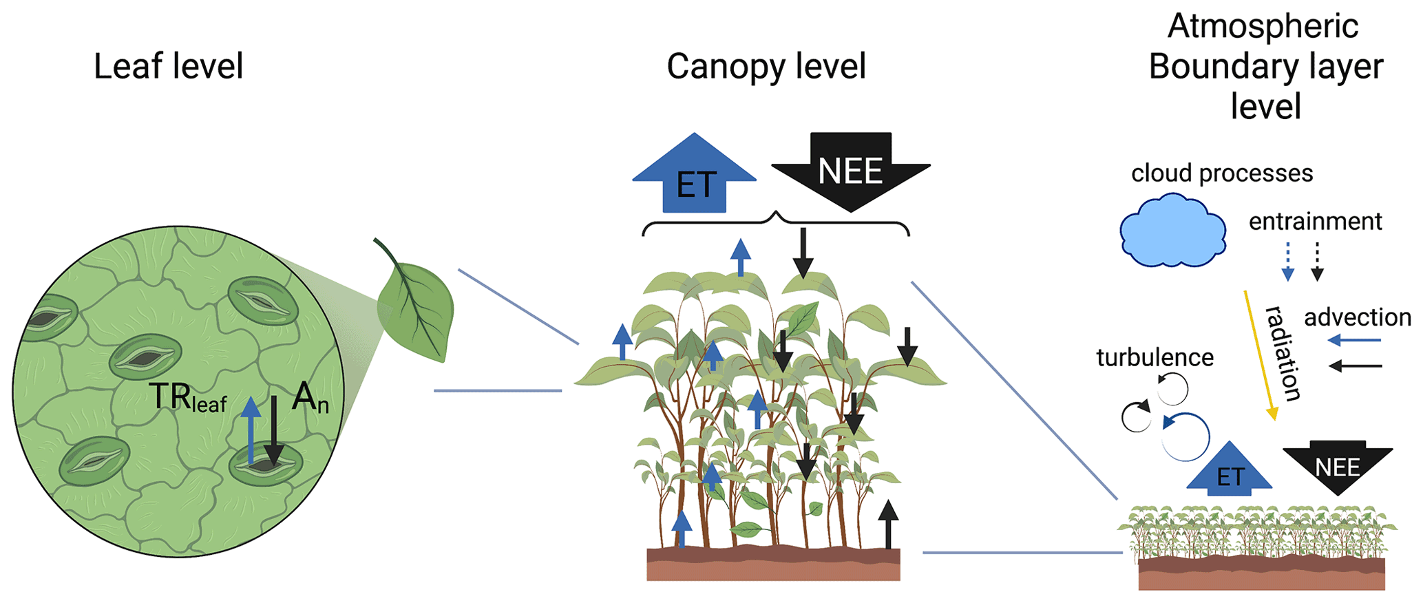
Figure 1Scheme of the three levels considered in the study of the exchange of water (represented by blue arrows) and carbon (represented by black arrows): (1) leaf level, (2) canopy level, and (3) ABL level. The exchanges of water and CO2 at the leaf level are represented by the leaf transpiration (TRleaf) and net CO2 assimilation (An), respectively. At the ABL level, several processes are included in the scheme such as advection of moisture and CO2 and entrainment of air from the free troposphere. Advection and entrainment of moisture and CO2 are indicated by solid arrows if they contribute to higher concentrations of water or CO2 in the ABL and by dashed arrows if they contribute to lower concentrations. In the scheme, we represent advection of moist and CO2-enriched air and entrainment of drier and CO2-depleted air from the free troposphere. The scheme was created with BioRender (https://www.BioRender.com; last access: 15 April 2024).
The objective of this research is to provide a framework with a new analytical method proposed for analyzing the diurnal dynamics of the fluxes of water and CO2. In particular, we aim to answer the following research question:
-
To what extent do the diurnal dynamics of environmental variables affect the diurnal dynamics of the water and CO2 exchange at the leaf and canopy levels?
Because processes interact across our three defined levels (leaf, canopy, and ABL levels), and together they shape the exchange of water and CO2, the framework combines observations and an encompassing model with representations at the leaf, canopy, and ABL levels. The analytical method entails the calculation of the tendency equations of the stomatal conductance, the leaf net CO2 assimilation, and the leaf transpiration. The tendency equations quantify the influence of temporal changes of four environmental variables on temporal changes of the leaf gas exchange. These four environmental variables are the photosynthetically active radiation (PAR), the air temperature (T), the vapor pressure deficit (VPD), and the atmospheric CO2 concentration (Ca). The quantification of their influence on the leaf gas exchange allows us to investigate which environmental variables control the dynamics of the exchange at different moments of the day. This framework was applied to an alfalfa crop in Spain over 1 day in summer 2021. To further explore the dependencies of the water and CO2 exchange on the environmental variables, three modeling experiments with ABL perturbations were analyzed.
2.1 LIAISE field campaign and definition of the case study
This research builds on the observations obtained as part of the field campaign Land surface Interactions with the Atmosphere over the Iberian Semi-arid Environment (LIAISE). LIAISE took place in the Ebro River basin in northeastern Spain with a special observation period (SOP) from 15 to 29 July 2021 with the overarching objective “to improve the understanding of land–atmosphere–hydrology interactions in a semi-arid region characterized by strong surface heterogeneity owing to contrasts between the natural landscape and intensive agriculture” (Boone et al., 2021). Further details about the field campaign and study site can be found in Boone (2019), Boone et al. (2021), and Mangan et al. (2023a).
La Cendrosa, our main study site, was one of the seven instrumented sites within the LIAISE domain. It was even considered a “supersite” since, in addition to standard energy balance and basic meteorology measurements, it also consisted of ABL measurements in the form of hourly launched radiosondes, ground-based remote sensing equipment, and a blimp with turbulence measurements. The crop grown at La Cendrosa is alfalfa, which was regularly irrigated through gravity-driven flood irrigation during LIAISE (on the nights of 10 and 23 July 2021).
Our research focused on the dynamics observed during the SOP on 17 July 2021. In this study, we express time series in coordinated universal time (UTC). In the region, local time (LT) is UTC +2. We chose to use UTC because, in this region, UTC aligns better with solar time, with 12:00 UTC roughly corresponding to solar noon. During the study day, there were no clouds present; there was light wind (≈2 m s−1 at 2 m height) and a maximum temperature of 32 °C. The synoptical condition was characterized by a thermal low-pressure system advecting warm and dry air to the study domain in the morning and early afternoon by light, westerly winds. In the late afternoon (after 18:00 UTC) a sea breeze front, the Marinada, came in from the east bringing cooler and moister air.
2.2 ABL level
2.2.1 CLASS model
The CLASS mixed-layer model (Vilà-Guerau de Arellano et al., 2015) was used to create the numerical modeling experiments. The CLASS model describes the ABL but it also contains a land surface scheme (Sect. 2.3.1) and a leaf gas exchange model (Sect. 2.4.1). A numerical experiment, referred to as the “control experiment”, was created to represent the study day and it was compared with observations. Details about the model initialization values of the control experiment and the land surface parameters are given in the following sections. Three additional numerical experiments based on the control experiment were created to explore the effect of various ABL perturbations on the local exchange of water and CO2 (Sect. 2.6).
Regarding how CLASS represents the ABL, CLASS is based on mixed-layer theory (summarized in Sect. 2.2 of Vilà-Guerau de Arellano et al., 2015), which states that atmospheric scalar variables are well mixed in height during the daytime, creating an atmospheric convective boundary layer (CBL). Consequently, the CBL can be described as a bulk layer, in which scalars (such as potential temperature, specific humidity, and CO2 concentration) are nearly constant with height and can be described by a single mixed-layer value. The interface between the CBL and the free troposphere is described as a sharp discontinuity in the scalars (e.g., potential temperature, humidity), normally called “scalar jump”. The free troposphere is described as a layer in which scalars change linearly with height. For instance, potential temperature increases at a constant lapse rate which is initially fixed in the experiment settings. CLASS also represents the surface layer (assumed to be the lower 10 % of the CBL) with Monin–Obukhov similarity theory (Monin and Obukhov, 1954), which allows for estimations of wind, temperature, and specific humidity at different heights in the surface layer. Because with CLASS we describe a CBL, our analysis during the study day started at 05:00 UTC, when the ABL was a CBL according to the vertical profiles of potential temperature measured by radiosondes. Our analysis was restricted until 15:40 UTC, when our numerical experiment indicated a transition to non-convective conditions.
2.2.2 Data and model initialization
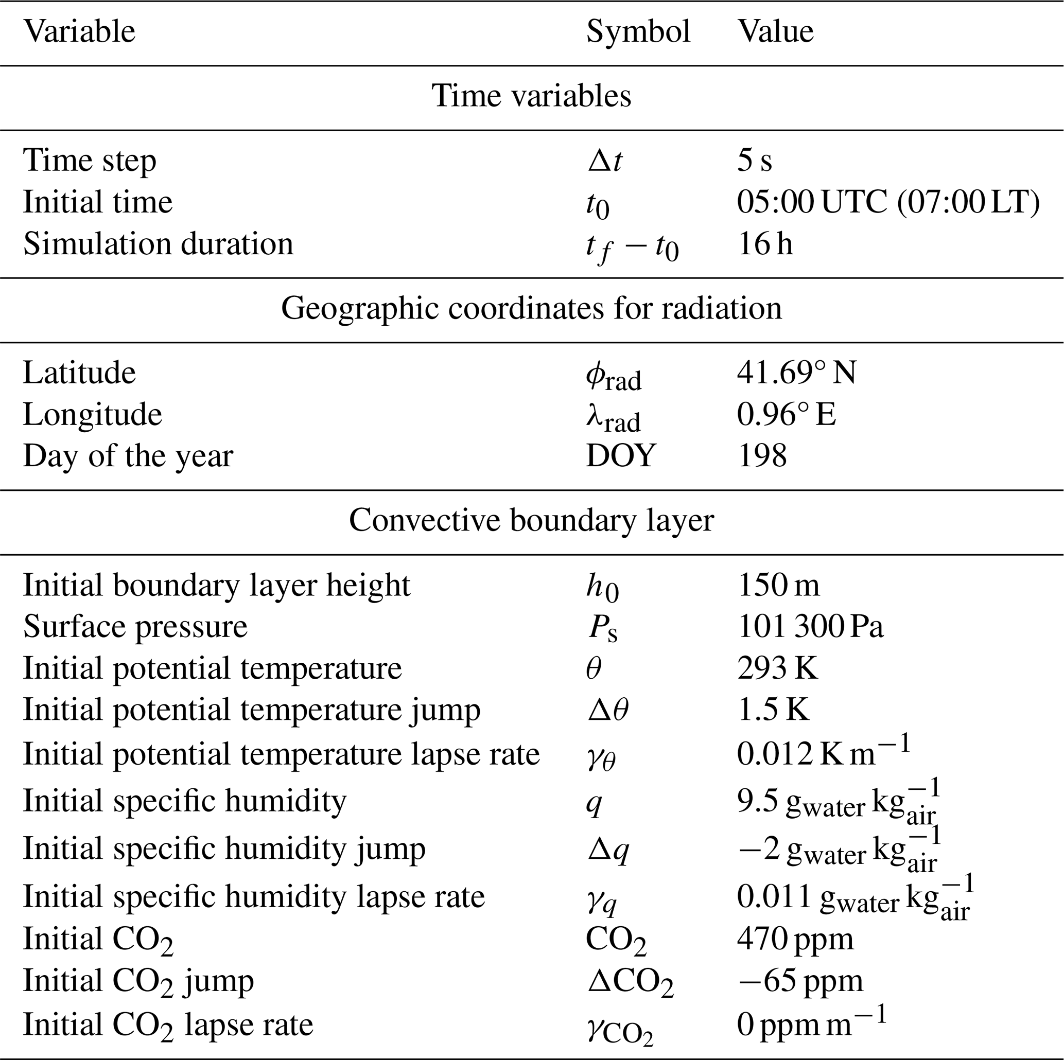
To characterize the ABL, vertical profiles of temperature, relative humidity, and wind obtained from radiosondes were used together with wind sensors located in a tower of 50 m height (at 10, 20, and 45 m). The radiosondes were released hourly from 04:00 to 17:00 UTC from the site. Radiosondes were used to provide the initial conditions for the numerical experiments (see Table 1 for exact values). Estimations of the CBL height were obtained from the radiosonde profiles using the parcel method (Kaimal and Finnigan, 1994). Mixed-layer values for potential temperature and specific humidity were obtained averaging the profiles below the boundary layer height minus a constant entrainment zone of 50 m and excluding the surface layer assumed to be the lower 10 % of the boundary layer. Lapse rates were obtained by calculating the slope of a linear regression of the vertical profile from 200 m above the top of the ABL to 3000 m height. Then, the jumps were calculated as the difference between the interpolated value at the boundary layer height and the mixed-layer value. Because the radiosondes did not measure CO2, we initialize the mixed-layer value with the value provided by the CO2 sensor that was part of an eddy covariance (EC) system located at 3 m height. Due to the lack of additional CO2 data, the initial jump of CO2 and the CO2 lapse rate were chosen in order to reproduce the magnitude of the diurnal variability in atmospheric CO2 measured by the EC system. Advection of heat and moisture was included based on estimations derived from a network of meteorological stations operated by the Servei Meteorològic de Catalunya, as calculated in previous research developed by Mangan et al. (2023a). The advective terms of the control numerical experiment can be found in Appendix A. Initial conditions for the CBL together with the time variables and the geographic coordinates needed for the initialization of radiation are given in Table 1.
Table 1General settings, radiation parameters, and initial conditions of CBL variables used in the control experiment.
2.3 Canopy level
2.3.1 Land surface scheme
CLASS represents the plant canopy as a homogeneous single layer of phytomass without vertical structure (often referred to as the “one big leaf” approach). That layer is represented by a bulk surface canopy conductance to water vapor (gsurf) or by its inverse, the surface canopy resistance to water vapor (). To obtain gsurf, the stomatal conductance to water vapor at leaf level (gs) calculated with the leaf gas exchange model of CLASS (the A-gs model; Sect. 2.4.1) is upscaled from the leaf to the canopy level. This upscaling is carried out by integrating gs over the leaf area and assuming an exponential decay of PAR with respect to leaf area index, as developed in Ronda et al. (2001). Then, to calculate ET the Penman–Monteith equation is used:
where Rn is the net radiation, G is the soil heat flux, qsat is the saturated specific humidity, is the well-mixed specific humidity, cp is the heat capacity of air at constant pressure, Lv is the latent heat flux of vaporization, ra is the aerodynamic resistance, and ρ is the air density.
NEE is calculated as the difference between the net CO2 rate assimilated by the vegetation canopy (Anc) and the soil respiration (Resp).
NEE is considered negative if CO2 is removed from the atmosphere and positive if CO2 is added to the atmosphere. Resp has the same sign convention, and it is always positive because it adds CO2 to the atmosphere. Unlike NEE and Resp, Anc is defined as positive if CO2 is removed from the atmosphere. Anc is derived with an approximation of Fick's law of diffusion, Eq. (3), that considers the difference between Ca and the intercellular CO2 concentration (Ci), the surface resistance, and the aerodynamic resistance. The Ci value is calculated with the A-gs model (presented in Sect. 2.4.1).
The factor of 1.6 accounts for the different molecular diffusivity of water vapor and CO2 (Jacobs and de Bruin, 1997).
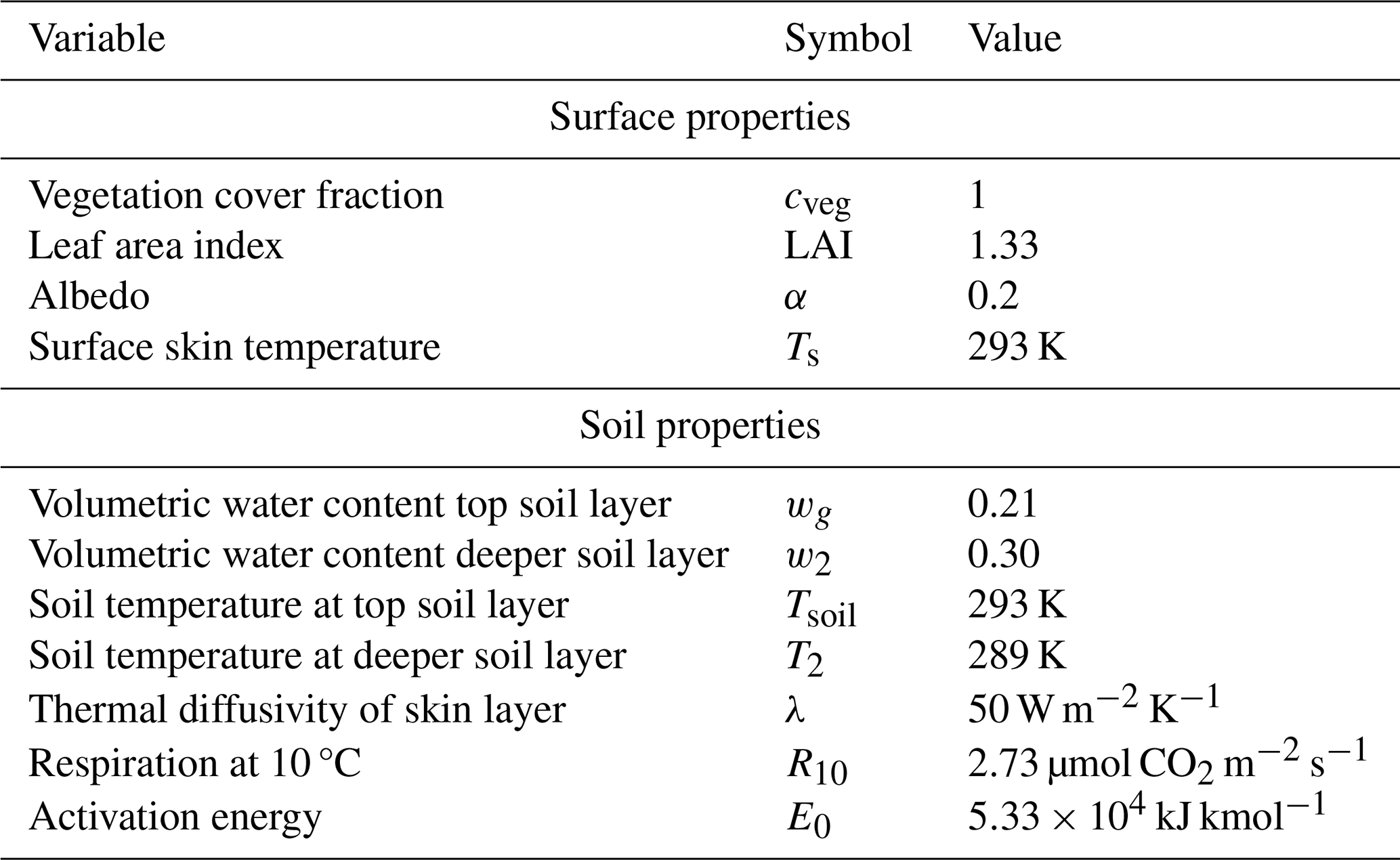
In the model, soil is represented with a two soil force–restore model as developed by Noilhan and Planton (1989) with a plant water stress function added by Combe et al. (2016). Soil respiration is parameterized as a function of soil temperature and soil moisture. The surface and soil parameters used for the control experiment are described in Table 2.
2.3.2 Data and model initialization
To characterize the canopy, we measured the leaf area index (LAI), the canopy height, and the time series of environmental variables (PAR, T, specific humidity, Ca, and wind), of soil respiration, and of the turbulent surface fluxes of water and CO2. We measured LAI with an LAI ceptometer (ACCUPAR LP-80). The instrument contains a PAR sensor to be deployed above the canopy together with a linear array of PAR sensors to be deployed inside the canopy. It calculates LAI considering the sun position and a spherical leaf angle distribution. We measured LAI between 10 and 12 times at different orientations in 12 locations at the La Cendrosa site. In total, we obtained 132 measurements for the study day with an average value of 1.33 and a standard deviation of 0.58. Similarly, we determined the canopy height by measuring 20 times at random locations in the field. The average canopy height was 28.5 cm with a standard deviation of 6.3 cm. We measured soil CO2 efflux with an SRC-2 soil respiration chamber connected to an EGM-5 portable CO2 gas analyzer. When measuring the soil CO2 efflux, we checked that no alfalfa plant was inside the chamber. In that way, no above-ground plant gas exchange would occur inside the chamber. We measured the soil CO2 efflux seven times throughout the day (from 07:15 to 19:00 UTC) near the EC tower. Every time, three or four soil CO2 efflux measurements were recorded. As a result, we obtain seven averaged values with their corresponding standard deviation.
Time series of environmental variables and fluxes were measured. PAR and Ca were measured above the canopy (at approximately 3 m), whereas temperature and specific humidity were also measured at different heights inside and right above the canopy. The sensible heat flux (H), latent heat flux (LE), and net ecosystem exchange (NEE) were measured at a surface station that was composed of an EC system (at 3 m height); four-stream radiometers, which measured net radiation (Rn); and ground heat flux (G) sensors. The average energy budget non-closure was calculated as . For more details about the set-up of the surface station, the reader is referred to Mangan et al. (2023a).
To compare model results and observations, we calculated the square of the Pearson correlation coefficient (r2), the p value, and the root mean square error (RMSE) between the model and the observed NEE and ET.
Table 2Surface and soil parameters used in the control experiment.
2.4 Leaf level
2.4.1 A-gs model
In the numerical experiments created with the CLASS model, we represented the leaf gas exchange with the A-gs model (Goudriaan et al., 1985; Jacobs, 1994). Details about the A-gs implementation used in CLASS can be found in Appendix A of Ronda et al. (2001) and in Appendix E of Vilà-Guerau de Arellano et al. (2015). The A-gs model calculates the internal CO2 concentration, the net assimilation rate (An), and the stomatal conductance to water vapor (gs) and to CO2 (gsc). Similar to Anc, An is defined as positive if CO2 is taken up from the atmosphere. An is calculated with the model developed by Goudriaan et al. (1985), which captures dependencies with PAR, T, and Ci and requires some parameters that describe the photosynthetic traits of the vegetation. Ci is calculated as a function of Ca, T, and VPD. To use the A-gs scheme in CLASS, five environmental variables are needed: PAR, T, VPD, Ca, and the soil water content at the root zone (w2). To represent the leaf level fluxes, we used the PAR received above the canopy (representing a sunlit leaf); the soil water content of the second layer of soil (deeper layer of soil from CLASS); and Ca, T, and VPD at 0.105 m height. Finally, we derived the leaf transpiration (TRleaf) taking into account gs and VPD.
2.4.2 Data and model initialization
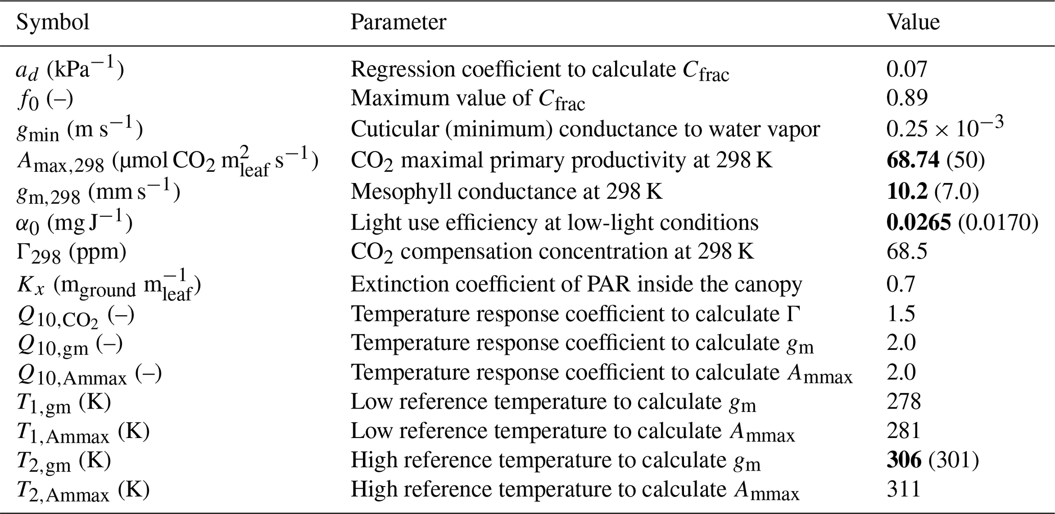
In terms of in situ plant ecophysiology observations, an LI-6400XT portable photosynthesis system was used to quantify the photosynthetic traits of the alfalfa crop and to measure the diurnal variability in gs. Photosynthetic traits were derived from photosynthesis response curves to PAR and to Ci, known as “A-PAR and A-Ci response curves”. Three A-PAR curves were measured at ambient temperatures ranging from 21 to 27 °C among the three curves and a constant ambient CO2 concentration of 400 ppm. The PAR approximate set points were 0, 10, 20, 40, 60, 120, 250, 500, 1000, 1200, and 1500 µmol photons m−2. Five A-Ci response curves were measured at saturating light (≈1500 µmol photons m−2) and ambient leaf temperatures ranging from 21 to 28.5 °C with Ci approximate set points of 50, 75, 100, 125, 175, 250, 400, 600, 800, 1000, and 1200 ppm. These measurements enabled the calculation of parameters that constrain the specific photosynthesis response of the alfalfa crop. The three fitted parameters, which are in the A-gs scheme, were (1) the CO2 maximal primary productivity at 298 K (Amax,298), (2) the mesophyll conductance at 298 K (gm,298), and (3) the light use efficiency at low-light conditions (α0). Finally, another parameter called the “high reference temperature” to calculate mesophyll conductance was increased to better reflect the warm growth conditions of the alfalfa crop. All the parameters of the A-gs model used in our study are indicated in Table 3. The observed and modeled response curves can be found in Appendix A.
The second types of measurements were diurnal time series of gs. We measured 221 leaves from 05:30 to 20:00 UTC. To mimic the field conditions we set PAR inside the chamber to the values measured outside. In practice, PAR values were updated in varying time steps of 15 min to 1 h to reflect the values measured by a PAR sensor located above the canopy. Based on the gs and on the in-canopy sensors present on the field, diurnal curves of TRleaf and An were derived. These measurements have been termed “post-processed observations”. The processing procedure is based on Fick's law of diffusion applied to the stomatal pores, assuming the thermal equilibrium between the air temperature measured inside the canopy and the leaves and a negligible leaf boundary layer resistance. Further details about the procedure to calculate the post-processing of observations can be found in Appendix A.
Similarly to the canopy level, we calculated r2, the p value and RMSE to compare model results and observations. Additionally, to facilitate the visual comparison of the time series, a simple moving average was computed by calculating an unweighted average considering the 15 previous and the 15 posterior observations for each leaf gas exchange data point.
Table 3Parameters of the A-gs model used for the numerical experiments. Parameters shown in bold font were modified from the default values used in the CLASS model (Vilà-Guerau de Arellano et al., 2015). For these modified parameters, the default values are shown within parentheses and in normal font.
2.5 Tendency equations for the leaf gas exchange
We derived tendency equations for the leaf gas exchange as a method for analyzing the temporal dynamics of the water and CO2 exchange. These equations describe the temporal evolution of the leaf gas exchange variables as a function of the time evolution of the environmental variables. Three tendency equations are proposed: (1) one for gs, (2) one for An, and (3) one for TRleaf. As a starting point to derive the tendency equations, we used the A-gs model (see Sect. S1 in the Supplement for a full derivation). Therefore, the set of environmental variables used in the tendency equations is the same as that used in the A-gs model, which is (1) PAR, (2) Ca, (3) VPD, (4) air T, and (5) w2. Because, according to our formulation, these five environmental variables control the leaf gas exchange, we refer to them as “environmental drivers” (of the leaf gas exchange). Although the tendencies were calculated considering all five environmental drivers, in this research we ignore the diurnal dynamics of w2, as w2 can be assumed constant in time in the root zone during the case study for La Cendrosa alfalfa field. This assumption was based on measurements of soil volumetric water content at 30 cm depth on the field, which showed a diurnal variation lower than 0.01 m3 m−3, and on the knowledge that the roots were likely to be deeper than 30 cm. The tendency equation for a leaf gas exchange variable Y (i.e., gs, An,l, or TRleaf) has the following form:
The left-hand side (LHS) of Eq. (4) describes the total rate of change in time of the generic leaf gas exchange variable Y. Taking as an example gs, this first term would indicate the rate of the opening or closure of the stomatal pores. The right-hand side (RHS) of the equation is composed of four terms which quantify the rate of change of Y due to temporal changes of PAR, T, VPD, and Ca. Using the same example of Y=gs, the terms would quantify the contribution to the total rate of the opening or closure of the stomatal pores that is attributed to the temporal changes of PAR, T, VPD, or Ca. For instance, the radiative term of the gs tendency equation in the morning would indicate how much of the stomatal opening is happening because radiation is increasing. Each of the terms on the RHS of the equation is the product of the partial derivative of Y with respect to a particular environmental driver (which gives information on the sensitivity of Y to a change in the environmental driver) multiplied by the total time derivative of the environmental driver. The sub-index notation for the T term (with VPD as sub-index) and for the VPD term (with T as sub-index) indicates that the partial derivatives were calculated considering the variable that appears as the sub-index to be constant. This notation was inspired in the thermodynamics notation for partial derivatives, and although it may seem redundant because of the definition of partial derivatives, it is deemed necessary to indicate that we considered T and VPD as independent variables. Another choice of independent variables was also possible. For instance, specific humidity or water vapor pressure could have been used in place of VPD. This is further explored in Sect. S1. As it is defined now, the temperature term only includes the plant physiological processes dependent on T such as the T dependency of mesophyll conductance and of maximal primary productivity. The total time derivatives of the environmental drivers were numerically derived from the modeling experiment output.
2.6 Three numerical experiments with ABL perturbations
Apart from the control experiment, three additional numerical experiments were performed. They were created to analyze how ABL processes that perturb the environmental drivers (i.e., PAR, T, VPD, and Ca) change the diurnal dynamics of water and CO2 exchange at the leaf and canopy levels. The new experiments were based on ABL processes that occurred at another time during LIAISE. The three experiments are (1) PAR-CLD, which represents surface radiative changes due to a cloud passage (Mol et al., 2023); (2) VPD-ENT, which represents entrainment of dry air masses from the free troposphere to the ABL (van Heerwaarden et al., 2009); and (3) TEM-ADV, which represents advection of cold air masses (Mangan et al., 2023a). Table 4 summarizes the type of perturbation of each experiment and the time when the perturbation was effective.
In the PAR-CLD experiment, surface PAR was reduced by about 25 % of its value at midday, representing the radiative effect of a cloud casting a shadow on the surface (Fig. 2a). The magnitude of the reduction of PAR was based on observations during another day of the campaign (24 July 2021; Fig. S2 in the Supplement) on which high clouds were present. In the VPD-ENT experiment, we imposed a drier free troposphere (compared with the control), which caused entrainment of drier air masses in the ABL (Fig. 2b). The magnitude of the mixing ratio in the free troposphere was 2 gwater kg drier than the control case and represented a range similar to the one investigated by van Heerwaarden et al. (2009). Finally, in the TEM-ADV experiment, we imposed strong cold air advection (Fig. 2c). The magnitude of the cold air advection ( K h−1 at its maximum) was based on the estimations of cold advection associated with the sea breeze that arrived in the region at 18:30 UTC during the study day (Mangan et al., 2023a; Fig. A1).
Table 4Numerical experiments in this study. The last three rows present the three experiments with ABL perturbations.
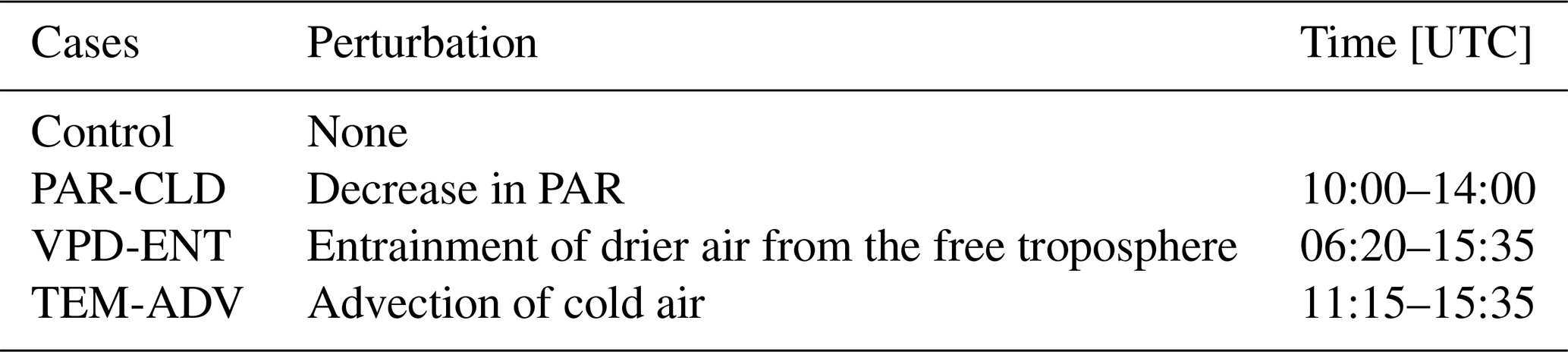
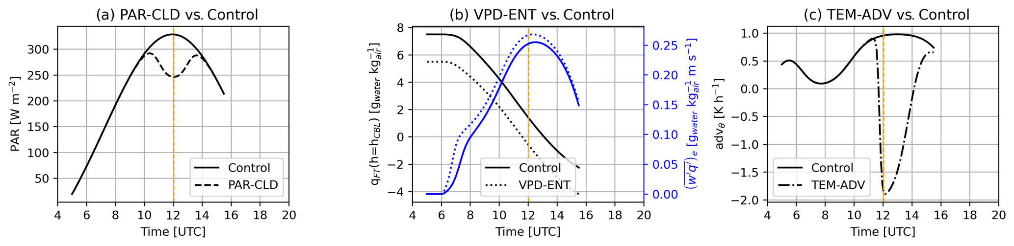
Figure 2Atmospheric changes imposed in the three perturbed experiments compared with the control simulation. Time series of (a) PAR for the PAR-CLD and control experiments, (b) specific humidity of tropospheric air and entrainment flux of specific humidity for the VPD-ENT and control experiments, and (c) temperature advection for the TEM-ADV and control experiments. Vertical dashed orange lines indicate solar noon.
To analyze the diurnal dynamics for the three perturbed numerical experiments, we compared the perturbed experiments against the control experiment in two ways: the first was to calculate the changes in the time-averaged leaf and canopy variables and the second was to compare the changes in the tendency terms.
The changes in the time-averaged variables were calculated as the mean percentage change of the leaf and canopy variables considering all the simulated hours. The mean percentage change, , represents the change in variable X of the ith experiment (expi) compared with the control experiment. It was calculated as follows:
where is the temporal mean of variable X, tini is the initial time, and tfin is the final time. was calculated for seven variables. The first three represented the leaf level: gs, An, and TRleaf. The second three were analogous variables but considering the whole canopy: gsurf, Anc, and ET. Lastly, we included -NEE to quantify the effects of the soil on the total carbon canopy flux. The negative sign applied to NEE was used to have the same sign convention as Anc. We did not consider the canopy transpiration (TRcanopy) because soil evaporation was negligible in our numerical experiments. As a consequence, ET was virtually equal to TRcanopy.
3.1 Control case
3.1.1 Environmental drivers of water and CO2 gas exchange
During the control day, there were no clouds and PAR was symmetric around solar noon (12:02:27 UTC), with a maximum value of 500 W m−2 (≈2200 µmol photons m−2 s−1; Fig. 3a). Observed Ca was 480 ppm at 04:00 UTC and decreased rapidly in the morning until 08:00 UTC when Ca stabilized around a relatively constant value of approximately 390 ppm (Fig. 3b). Observed potential temperatures varied among the heights inside (0.105 m) and above the canopy (3 m and mixed-layer value; Fig. 3c). Inside the canopy, the maximum potential temperature was acquired sooner than above the canopy. VPD was found to increase with height, reaching a maximum difference of approximately 1000 Pa between 0.105 and 3 m (Fig. 3d). The model captured the diurnal and height-dependent variability observed for the environmental drivers except for Ca. For Ca the model captured the magnitude of the diurnal variability but failed to capture its dynamics. Modeled Ca decreased at a lower pace than observed Ca. As a consequence, modeled Ca was larger than observed Ca, particularly in the morning. To explore the implications of this mismatch in our results, we carried out an additional numerical experiment (Sect. S3). Possible explanations of the mismatch are discussed in Sect. 4.
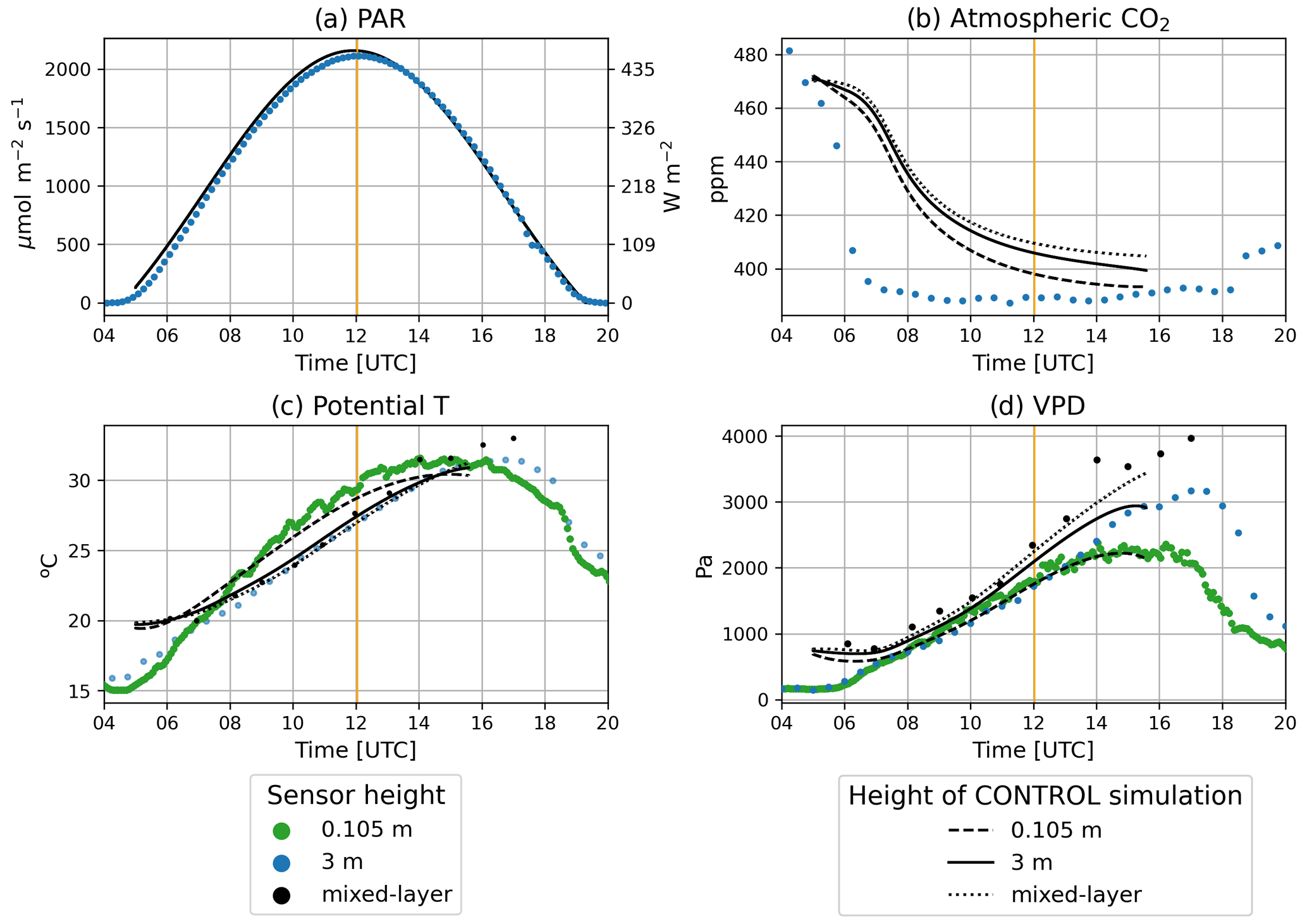
Figure 3Diurnal time series of (a) PAR, (b) Ca, (c) potential temperature, and (d) VPD. Observations are depicted by dots. The sensor at 0.105 m height is located inside the canopy. Black dots show potential T and VPD derived from radiosondes. The solid black line corresponds to the control experiment at 3 m, and the dashed line corresponds to the control experiment at 0.105 m; the dotted line is the mixed-layer value. Vertical orange lines depict the solar noon. Direct and diffuse components of radiation can be found in Fig. S1.
3.1.2 Leaf gas exchange
Observed gs showed the highest values in the morning, reaching a maximum value of approximately 0.020–0.030 m s−1 (≈1.00–1.20 molair m s−1) at 10:00 UTC and declining afterwards until the end of the day (Fig. 4a). Modeled gs was at a maximum at the same time as the observed gs and showed a relatively weak but significant correlation with the observations (r2=0.223, p<0.001). Observed and modeled An followed closely the diurnal pattern of PAR (Fig. 3a), achieving maximum values approximately at solar noon between 12:00 and 13:00 UTC (Fig. 4b). Model results showed a significant correlation with the post-processed observations (r2=0.383, p<0.001). Finally, TRleaf also increased in the morning and decreased in the afternoon, with a maximum value achieved towards the afternoon between 12:45 and 14:00 UTC (Fig. 4c). Model results showed a significant and high correlation (r2=0.677, p<0.001) with post-processed observations, although model results overestimated maximum TRleaf compared with the post-processed observations. Comparing the modeled leaf gas exchange variables with the observed moving averaged variables, we noticed that the diurnal pattern is well captured, thus suggesting that the relatively low correlations were partly due to the scatter of observations. A more elaborate comparison of the observations and model results of the leaf gas exchange can be found in Sect. S4.
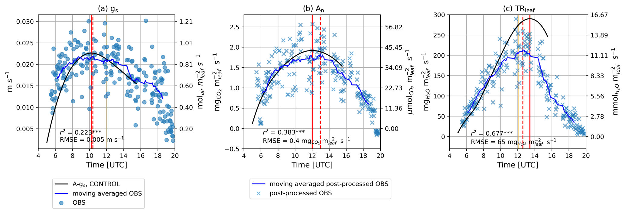
Figure 4Diurnal time series of (a) gs, (b) An, and (c) TRleaf for the control experiment. Direct observations are depicted by blue dots, whereas post-processed observations are depicted by blue crosses. Moving averaged observations and post-processed observations are indicated with a blue line. Model results of the control experiment are depicted by solid black lines. Vertical solid orange lines depict solar noon. The time when the maximum value of the leaf gas exchange variable at hand was achieved is depicted by vertical solid red lines for model results and vertical dashed red lines for observations or post-processed observations.
3.1.3 Canopy level gas exchange
Observed NEE was positive before 06:00 UTC, indicating a net transport of CO2 from the surface to the atmosphere (Fig. 5a), which suggests that ecosystem respiration was providing CO2 to the atmosphere. From 06:00 to 18:00 UTC, the observed flux was negative, acquiring a minimum value between 11:00 and 12:00 UTC. The diurnal negative NEE indicated a net transport of CO2 from the atmosphere to the surface, suggesting that the photosynthesis of the crop was dominant over respiration processes. Modeled NEE had a strong and significant correlation with observations (r2=0.89 and p<0.001). Additionally, the time at which the minimum NEE was attained matched well between observations and model results. Observed soil respiration was between 4.5 and 9 µmol m−2 s−1 during the day, which coincided with the range reproduced by the model. Observed ET reached a maximum value of 6.5 mmol m−2 s−1 that stayed relatively constant between 11:00 and 15:00 UTC. This plateau was not reproduced by the model, which peaked at approximately 12:45 and then declined. Similar to the observation at leaf level, modeled ET was higher than observed ET. The overestimation of modeled ET was of the same magnitude as the observed energy budget non-closure. Despite the apparent differences, modeled ET had a strong and significant correlation with observed ET (r2=0.95 and p<0.001) (Fig. 5).
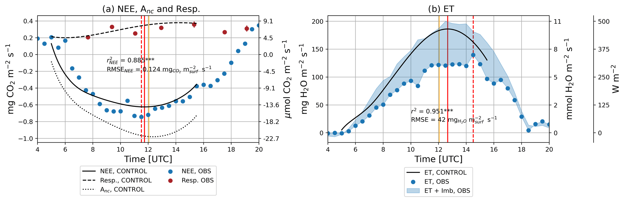
Figure 5Diurnal time series of (a) NEE, −Anc, and soil respiration (Resp.) and of (b) ET and latent heat flux (LE). The 30 min averaged observations from the EC system are depicted by blue dots, whereas model results are depicted by different line styles. Respiration observations are depicted by red dots with an error bar that represents the standard error of the mean. The measured surface energy budget non-closure is represented by a shaded space covering the area from the measured ET or LE value to the measured ET or LE value plus the measured surface energy budget non-closure. Vertical solid orange lines depict solar noon. The times when the maximum of NEE and ET was achieved are depicted by vertical solid red lines for model results and vertical dashed red lines for observations or post-processed observations.
3.1.4 Tendencies of the leaf gas exchange
The total tendencies of gs, An, and TRleaf (LHS of Eq. 4) described the diurnal dynamics observed in the modeled leaf gas exchange variables (Sect. 3.1.2). These dynamics consisted of an increase in the leaf gas exchange variables (positive total tendency term) until reaching a maximum (null total tendency term), which occurred in the morning for gs, at noon for An, and in the afternoon for TRleaf, followed by a decrease until the end of the simulation time (negative total tendency term). The sum of the partial tendency terms (RHS of Eq. 4) matched exactly the total tendency term (LHS of Eq. 4) for gs, An, and TRleaf (see the overlapping of the solid black line and the dashed gray line in Fig. 6a, b, and c). This verification guaranteed that the temporal evolution of gs, An, and TRleaf was fully determined by the temporal evolution of PAR, T, VPD, and Ca. Focusing on the partial terms, the radiative terms (PAR terms) were found to be the primary contribution to the total terms of the leaf gas exchange variables, especially for gs and An. The temporal changes in PAR tended to increase the leaf gas exchange variables before noon (positive PAR terms) and to decrease them after noon (negative PAR terms). The T, VPD, and Ca terms added secondary temporal dynamics to the contribution of the PAR terms.
For gs (Fig 6a), the VPD term was negative from 07:00 to 15:00 UTC, indicating that the diurnal increase in VPD (Fig. 3d) led to smaller gs values. This effect was partially compensated by the T and Ca terms, which were both positive. Therefore, both the increase in T due to the diurnal warming of the atmosphere (Fig. 3c) and the decrease in Ca due to the entrainment of CO2-depleted air from the free troposphere (Fig. 3b) contributed to increased gs. The net effect of these opposing terms resulted in the maximum of gs being achieved 2 h before solar noon. For An (Fig. 6b), the diurnal increase in T favored higher An values, increasing the An rate especially in the morning (positive T term). Both the VPD and Ca terms were relatively small compared with the PAR and T terms, which suggested that the diurnal dynamics of An were relatively insensitive to diurnal changes in VPD and Ca. Finally, for TRleaf (Fig. 6c), the T, VPD, and Ca terms tended to further increase TRleaf values. The T and VPD terms were found comparable and greater than the PAR term for several hours in the morning and early afternoon. The combined effect of the T, VPD, and Ca terms was responsible for delaying the maximum TRleaf from occurring at solar noon (if the model would be sensitive only to PAR temporal changes) to 13:30 UTC. The results of the partial tendency terms highlighted that diurnal temporal changes in PAR primarily forced the net diurnal dynamics of the leaf gas exchange variables, whereas diurnal temporal changes in Ca were found to be the least important factor for describing the leaf gas exchange dynamics.
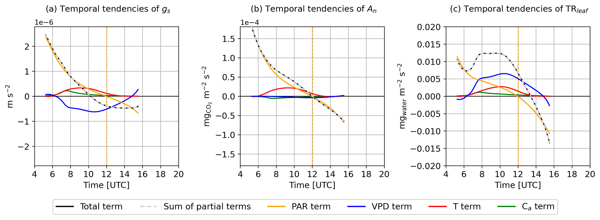
Figure 6Temporal evolution of the tendencies of (a) gs, (b) An, and (c) TRleaf. Black lines depict the total tendency terms, dashed gray lines depict the sum of the partial terms, and the other solid colored lines depict the partial tendency terms due to temporal changes in PAR (orange lines), VPD (blue lines), T (red lines), and Ca (green lines). The vertical dashed orange lines depict solar noon.
3.2 Three experiments with ABL perturbations
3.2.1 Environmental drivers of water and CO2 gas exchange
The three experiments with ABL perturbations (PAR-CLD, VPD-ENT, and TEM-ADV) modified the environmental drivers of the water and CO2 exchange compared with the control simulation, except for Ca, which remained almost equal to the control for all the perturbed experiments (Fig. 7a). The PAR-CLD experiment described a cloud passage which reduced surface PAR (Fig. 2a). The cloud passage also modified the surface energy balance during and after the cloud shade. As a consequence, T and VPD were reduced by up to 1 K and 250 Pa, respectively (Fig. 7b and c). The VPD-ENT experiment, which described a drier free troposphere than the control experiment, only modified VPD, which increased by up to 250 Pa (Fig. 7c). Lastly, the TEM-ADV experiment, which described strong cold air advection, reduced not only T by up to 4 K but also VPD by up to 1000 Pa (Fig. 7b and c).
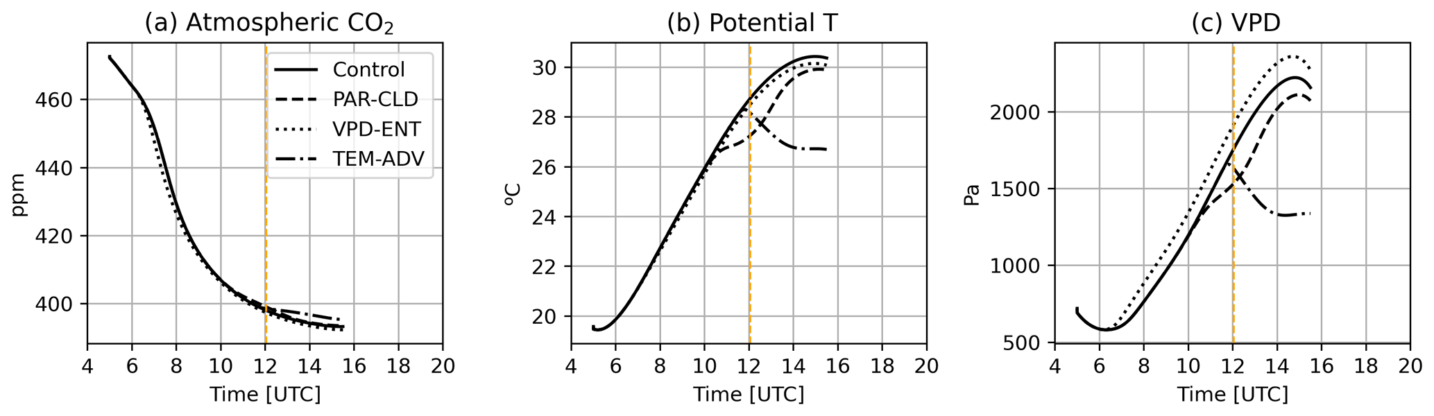
Figure 7Temporal evolution of (a) Ca, (b) potential T, and (c) VPD at 0.105 m for the four experiments. The solid black line corresponds to the control experiment, the dashed black line to the PAR-CLD experiment, the dotted black line to the VPD-ENT experiment, and the dash-dotted black line to the TEM-ADV experiment. Vertical dashed orange lines depict solar noon.
3.2.2 Leaf and canopy gas exchange
Compared with the control experiment, the changes in the environmental drivers led to changes in the leaf and canopy variables that describe the water and CO2 exchange. The mean values of the exchange variables changed by up to 11 % compared with the control experiment (Fig. 8). For PAR-CLD, there was a slight reduction in stomatal conductance and surface conductance (, ), a moderate reduction in the assimilated CO2 by the vegetation (, ), and a strong reduction in the water exchange at the leaf and canopy levels (, ). For VPD-ENT, a moderate reduction in stomatal conductance and surface conductance was reported (, %), whereas TRleaf and ET were moderately increased (, PET>3 %). An and Anc barely changed compared with the control experiment (, ). Lastly, for TEM-ADV there was a strong increase in stomatal conductance and surface conductance (, ), a strong decrease in TRleaf (), and a moderate decrease in ET (). Similar to the VPD-ENT experiment, An and Anc barely changed in comparison with the control simulation (, ).
When comparing the experiments, all of them modified moderately or strongly TRleaf and ET, whereas only the PAR-CLD experiment modified moderately An and Anc. Comparing the trends between leaf and canopy levels for each experiment (gs versus gsurf, An versus Anc, and TRleaf versus ET), we generally observed similar patterns in the magnitude and sign of the change between the leaf- and canopy-level variables, with two remarkable exceptions. The first exception was the small decrease in An at leaf level as opposed to a small increase in Anc at canopy level for the VPD-ENT experiment compared with the control. Further analysis revealed that the decrease in VPD for VPD-ENT led to a reduced Ci, which affected the CO2 exchange differently at the leaf level and canopy level. At leaf level, the decrease in Ci implied lower maximum rates of photosynthesis because less CO2 was available to perform photosynthesis, which finally led to a smaller net assimilation rate. However, at canopy level, the decrease in Ci was accounted for with a diffusion type of equation (Eq. 3), which resulted in a higher Anc due to a higher CO2 gradient (Ca-Ci). The second unexpected result was the large decrease in TRleaf at leaf level compared with the moderate decrease in ET at canopy level for TEM-ADV. Further exploration revealed that the change in magnitude was partially attributed to the effect of the wind in the exchange which was only accounted for at canopy level. Although horizontal wind was equal for all experiments, the vertical component was greater for TEM-ADV than for the control, which implied a smaller aerodynamic resistance and favorable conditions for the exchange of water for TEM-ADV with respect to the control. This effect was partially responsible of a smaller decrease in ET than in TRleaf.
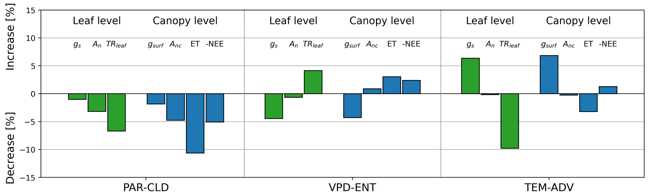
Figure 8Bar plot of the mean percentage change in seven leaf and canopy variables of the perturbed experiments with respect to the control experiment. The set of variables is composed of three leaf gas exchange variables (gs, An, and TRleaf), indicated by green bars, and by four canopy gas exchange variables (gsurf, Anc, ET, and -NEE) in blue bars.
3.2.3 Tendencies of the leaf gas exchange
Analyzing the tendency terms of the three perturbed ABL experiments showed a clear separation between the effects of the environmental drivers on An and TRleaf (Fig. 9). The reduction in An for the PAR-CLD experiment (Fig. 9a) followed closely the shape of the decrease in PAR, which occurred roughly between 10:00 and 12:00 UTC (Fig. 2a). Accordingly, the difference in the net total tendency terms between PAR-CLD and control followed closely the difference in the radiative terms (Fig. 9b). This suggests that the dip in An was mostly attributed to the radiative changes. As a second-order effect, the difference in the temperature terms indicated that the temperature variability during the cloud passage also contributed to reducing An. For VPD-ENT and TEM-ADV, the An diurnal dynamics remained quite similar to those of the control, and hence the differences in the tendency terms were much smaller than those of PAR-CLD.
Similar to the reduction in An for PAR-CLD, the reduction in TRleaf for the PAR-CLD (Fig. 9e) experiment was strongly influenced by the reduction in radiation (Fig. 9f). However, in this case both the temporal dynamics of temperature and VPD during the cloud passage contributed to the reduction in TRleaf (Fig. 9f). For the VPD-ENT experiment, TRleaf was higher than in the control between 06:00 and 07:00 UTC and at the end of the simulation. The difference in the total tendency term was very similar to the difference in the VPD term, indicating that the VPD diurnal variability was responsible for the increase in TRleaf (Fig. 9g). Lastly, TRleaf for the TEM-ADV experiment was strongly reduced compared with the control experiment after the advection started (Fig. 9e). This reduction resulted from the contribution of the reduction both in VPD and T, with the dynamics of VPD being roughly 3 times more important than the dynamics of temperature (Fig. 9h). Interestingly, our tendencies showed that PAR contributed positively to An and TRleaf during the advection of cold air (Fig. 9d and h), even though the PAR diurnal variability remained unchanged compared with the control experiment. The positive value of the difference in PAR tendency terms for TRleaf indicated that temporal changes in radiation were contributing less to the decrease in TRleaf in TEM-ADV compared with the control. This effect was related to the lower contribution of radiative variability to the changes in stomatal conductance, which were predominantly influenced by the drop in VPD.
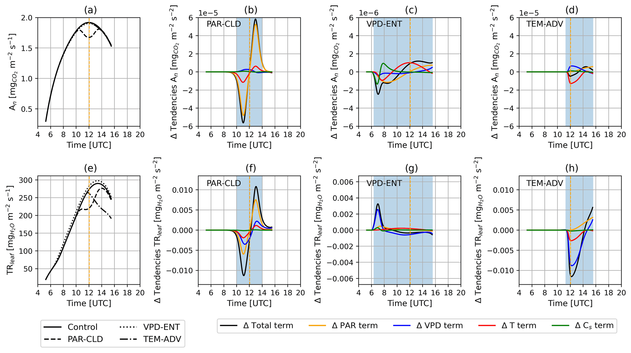
Figure 9Diurnal evolution of (a) An and (e) TRleaf for the control (solid black line), PAR-CLD (dashed black line), VPD-ENT (dotted black line), and TEM-ADV (dash-dotted black line) experiments. Diurnal evolution of the difference in An tendency terms of each perturbed experiment against the control experiment is shown in (b) for PAR-CLD, (c) for VPD-ENT, and (d) for TEM-ADV. The diurnal evolution of the difference in TRleaf tendency terms between each perturbed experiment against the control experiment is shown in (f) for PAR-CLD, (g) for VPD-ENT, and (h) for TEM-ADV. Note that the difference in the tendency terms for the VPD-ENT experiment is smaller than for the PAR-CLD and TEM-ADV experiments. Because of that, the y axis in Fig. 9c is 10 times smaller than the y axis in (b) and (c), and the y axis in (g) is half the y axis in (f) and (h). Solar noon is indicated with a vertical dashed orange line. Time periods when the ABL perturbations were effective are shown as blue shades in panels (b), (c), (d), (f), (g), and (h).
The framework proposed in this research was constituted by observations and a coupled model with descriptions at leaf, canopy, and ABL levels and by tendency equations of the modeled leaf gas exchange (for net assimilation rate, stomatal conductance, and leaf transpiration). Our research strategy resembled that of Vilà-Guerau de Arellano et al. (2020) and Mangan et al. (2023a), in that a range of spatial scales were integrated to investigate the diurnal variability of turbulent fluxes. Additionally, a key element of the study is the comprehensiveness of the measurements (leaf gas exchange observations, surface turbulent fluxes, and atmospheric boundary layer observations), which is considered suitable to progress to the investigation of the vegetation/ecosystem response to meteorological conditions and the effect of ecosystem responses on the atmospheric dynamics (land–atmosphere bi-directional feedbacks) (Helbig et al., 2021).
In this study, the coupled model CLASS was able to reproduce the observed diurnal variability of the environmental drivers for the study day except for the variability in Ca (Fig. 3b). Unlike for VPD and T, Ca measurements were only available at 3 m, and we did not have information about its vertical variability. The CLASS model assumes that Ca is well mixed from the start of the numerical experiment. However, Ca vertical profiles can depict strong vertical gradients during and after the morning transition from a stable ABL to an unstable and well-mixed ABL, as has been previously observed over grass (Casso-Torralba et al., 2008). As a consequence, the initial observed Ca values may not be representative of the initial convective ABL. To explore the impact that the mismatch between modeled and observed Ca had on our results, we performed an additional numerical experiment in which modeled Ca resembled closely observed Ca (Sect. S3). We found that the leaf gas exchange tendencies retained their main features, and they led to the same conclusions of the study.
Regarding the leaf level, observations of stomatal conductance were scattered, which led to scatter in the post-processed observations of net assimilation rate and leaf transpiration (Sect. 3.1.2). This showed that randomly picked leaves within the alfalfa canopy at a same moment of the day gave values of stomatal conductance that differ from each other. We attribute this spread to the different environmental conditions experienced by each leaf (e.g., sunlit and shaded leaves) and to differences in leaf properties (e.g., age or damage of leaves). Similar dependencies of leaf gas exchange on the sun or shade preconditioning of leaves and on the age of the leaves have been previously reported for a cotton crop by Echer and Rosolem (2015). Our modeled results did not represent this variability, as they were based on a single combination of the modeled PAR, atmospheric CO2, T, and VPD per time during the day and the same photosynthetic traits for all leaves. Despite the scatter, the moving averaged observations presented a magnitude and diurnal characteristics that were consistent with the model results such as the time of occurrence of maximum values.
Based on the modeled leaf gas exchange, tendency equations were used to quantify the effect of the diurnal dynamics of the environmental drivers on the dynamics of the leaf gas exchange. In that regard, the tendency terms informed about the modeled leaf gas exchange and are bounded by the assumptions of the same. An addition that could be made to the A-gs scheme is the temporal adaptation of the stomata to instantaneous changes in environmental conditions (Sellers et al., 1996; Vico et al., 2011; Sikma et al., 2018). Adaptation of the stomata could be important especially for fast radiative perturbations such as those that have been observed and modeled in previous research (Kivalov and Fitzjarrald, 2018; Mol et al., 2023) during cloudy days. Another feature that was not accounted for in the numerical experiments was the partitioning of shortwave radiation between its direct and diffuse components. This partitioning can be important because diffuse light is considered to increase the portion of the vegetative canopy that receives illumination, and therefore it can increase the net CO2 assimilated by the canopy (Niyogi et al., 2004; Knohl and Baldocchi, 2008). During the LIAISE field campaign, direct and diffuse components of shortwave radiation were measured at La Cendrosa (Figs. S1 and S2). During the study day, the ratio of diffuse radiation to the net radiation was approximately 15 %, categorized as a low diffusive regime according to Niyogi et al. (2004). Therefore, we anticipate minimal impact of the partitioning of the direct and diffuse components for the control experiment, on which we based the largest part of our conclusions. For the VPD-ENT and TEM-ADV numerical experiments, the partitioning of radiation remains consistent, suggesting a minor impact on our results. However, for the PAR-CLD numerical experiment, the ratio of diffuse radiation to the net radiation could substantially change compared with the control because of the cloud. On a cloudy day during the campaign, the ratio of diffuse radiation to net radiation oscillated between 35 % and 100 % (Fig. S2), with values larger than 60 % being categorized as highly diffusive according to Niyogi et al. (2004). Such cloud-induced changes in direct and diffuse partitioning could influence the CO2 exchange, potentially leading to larger canopy CO2 uptake in PAR-CLD compared with our results. For instance, Pedruzo-Bagazgoitia et al. (2017) found greater (up to 9 %) net assimilation of CO2 under thin clouds (with a cloud optical depth smaller than 3) than under clear sky in large-eddy simulations. We emphasize that the direct and diffuse partitioning is relevant for understanding the vertical profiles of light within the canopy, and therefore it is considered when upscaling fluxes from leaf level to canopy level. However, the leaf tendencies as they have been presented here could still be coupled with a model that accounts for direct and diffuse partitioning.
Tendency equations, similar to the ones presented here, have been proposed in the past for leaf transpiration (Jarvis and McNaughton, 1986), evapotranspiration (van Heerwaarden et al., 2010), and net ecosystem exchange (Pedruzo-Bagazgoitia et al., 2017) but with substantial differences with respect to our study. Jarvis and McNaughton (1986) used a similar approach to investigate the dependency of transpiration on stomatal conductance for scales ranging from 10−5 to 105 m. The approach was different because it was not intended to analyze the temporal dynamics of the fluxes but to investigate the sensitivity of transpiration on stomatal conductance at different scales. Because of that, Jarvis and McNaughton (1986) used differential equations but not with respect to time. Additionally, the CO2 fluxes were not investigated, and to the authors' knowledge, this is the first time that the tendencies have been calculated simultaneously for stomatal conductance, leaf transpiration, and net assimilation rate, providing a complete view of the leaf gas exchange. On the other hand, van Heerwaarden et al. (2010) calculated tendency equations for the canopy evapotranspiration and Pedruzo-Bagazgoitia et al. (2017) for the net canopy CO2 assimilation. Both groups applied the approach to investigate diurnal dynamics in realistic field conditions. The approach of van Heerwaarden et al. (2010) was based on the Penman–Monteith equation combined with mixed-layer theory for CBL, whereas the approach by Pedruzo-Bagazgoitia et al. (2017) was based on the upscaled CO2 flux given by A-gs (Eq. 3). The main difference between those approaches and the one presented here is that we calculated the terms as a function of state primary variables, whereas van Heerwaarden et al. (2010) and Pedruzo-Bagazgoitia et al. (2017) did so for intermediate variables. For example, a term of the equation proposed by Pedruzo-Bagazgoitia et al. (2017) contained the temporal derivative of Ci, which may be more difficult to interpret and relate to environmental processes than changes in PAR, T, VPD, and Ca. We acknowledge that for certain research questions it may be relevant to use a different subset of independent variables. However, the choice of another subset is also possible within the proposed framework. Finally, we would like to comment on the possibility of combining tendency equations and observations. Whereas the previously cited research calculated tendencies with models, Mangan et al. (2023b) calculated the LE tendencies derived by van Heerwaarden et al. (2010) and applied them to the coupled model CLASS but also to observations. By doing so, they could explore whether the model and observations agreed that certain processes impact LE in the same manner. In principle, a similar approach could be developed for the tendencies introduced in the current paper. Although observations will introduce a large scatter to the tendencies, a comparison between tendencies of the leaf gas exchange applied to models and observations could provide an additional tool for assessing the performance of the A-gs scheme apart from directly comparing leaf fluxes.
Returning to the initial research question (To what extent do the diurnal dynamics of environmental drivers affect the diurnal dynamics of the water and CO2 exchange at leaf and canopy levels?), we observed that the dynamics of stomatal conductance and net assimilation rate were primarily forced by the diurnal dynamics of radiation. As a second-order effect, the dynamics of net assimilation rate were affected by those of T and the dynamics of stomatal conductance by those of T and VPD. Leaf transpiration was affected to a similar extent by the dynamics of PAR, T, and VPD, with PAR dynamics being the most important factor in the early morning and late afternoon. The leaf gas exchange dynamics were less sensitive to the dynamics of atmospheric CO2 concentration than to the dynamics of PAR, T, and VPD. These results indicate that radiative perturbations (such as those created by cloud shade) strongly affect the diurnal evolution of the assimilation rate, a fact that was further explored in the PAR-CLD experiment. In fact, from all the experiments, PAR-CLD was the one that modified most the net CO2 assimilation rate, suggesting that the representation and understanding of clouds and their effects on the surface are a crucial factor for understanding and representing the diurnal variability in CO2 fluxes (Vilà-Guerau de Arellano et al., 2023). Additionally, the PAR-CLD experiment showed that not only radiative changes but also associated temperature changes produced by a cloud shade can further reduce the net assimilation rate. Although the other experiments which represented entrainment of drier air and advection of cold air (VPD-ENT and TEM-ADV) did not significantly modify the net assimilation rate and gross primary productivity, they did modify the stomatal conductance, surface conductance, leaf transpiration, and evapotranspiration. Similar to what was reported by van Heerwaarden et al. (2009), entrainment of dry air under non-stressed soil water availability (VPD-ENT experiment) enhanced the water surface exchange. Lastly, the cold air advection experiment (TEM-ADV experiment) suggested that heat advection modifies leaf transpiration not only because the temperature changes but also due to the associated VPD changes.
To close the discussion, we mention some possible avenues for future work. We envision that the tendency equations can help to identify errors and shortcomings and to investigate limiting factors of the water and CO2 exchange, represented in global models that explicitly include vegetation (Doutriaux-Boucher et al., 2009), in standard weather and climate land–surface models (Renner et al., 2021), and/or in new-generation models such as land–surface models with a multi-layer canopy (Bonan et al., 2021). One possible application of the method is to investigate the dependency of the temporal dynamics of the leaf gas exchange on soil moisture during a dry spell (Combe et al., 2016) or during and after a precipitation event. Soil moisture tendencies were not investigated in this paper because the alfalfa crop leaf gas exchange was not limited by its root soil water content. However, our modeling framework enables the calculation of the soil water content tendency. In principle, the tendency equations can be applied to timescales larger than 1 day such as weekly or monthly scales. Another application of the tendencies could be to analyze how the relations between the environmental drivers and the leaf gas exchange vary vertically inside a canopy. For instance, this analysis could help in understanding the causes of the different magnitudes of the fluxes in the layers of a forest (e.g., understory versus top of the canopy). For this, the method could be applied to different layers within a multi-layer canopy (Bonan et al., 2021; Pedruzo-Bagazgoitia et al., 2023). Lastly, we would like to mention that the tendencies can be calculated with the output of models if the necessary variables have been saved. Because of that, this interpretative tool is not computationally expensive once the model has been run.
In this research, we investigated the leaf and canopy exchange of water and CO2 and its relationship with the diurnal dynamics of four environmental variables – photosynthetic active radiation (PAR), air temperature (T), vapor pressure deficit (VPD), and atmospheric CO2 concentration (Ca) – for an irrigated alfalfa field. We based the research on 1 day during the field campaign Land Surface Interactions with the Atmosphere in the Iberian Semi-Arid Environment (LIAISE). We created a numerical control experiment based on the study day with a mixed-layer model (CLASS model; Vilà-Guerau de Arellano et al., 2015) that represents the convective atmospheric boundary layer (ABL) level, the canopy level, and the leaf level (with the A-gs model; Goudriaan et al., 1985; Jacobs, 1994). In terms of observations, the leaf gas exchange was characterized with observations carried out with an LI-6400XT Portable Photosynthesis System. The canopy gas exchange was characterized with 30 min averaged eddy covariance (EC) measurements and soil respiration measurements. To quantify the contributions of the diurnal dynamics of the environmental variables (PAR, T, VPD, and Ca) to the water and CO2 exchange, we derived three tendency equations for stomatal conductance, net assimilation rate, and leaf transpiration. To investigate the effects of ABL processes on the local exchange, we created three additional numerical experiments with three ABL perturbations: (1) a reduction in surface radiation due to a cloud shade, (2) entrainment of drier air masses from the free troposphere, and (3) a strong cold air advection. We ascertain that the partial tendency terms of the leaf gas exchange fully accounted for the diurnal dynamics of the leaf gas exchange. An important finding was that PAR diurnal dynamics strongly influenced the diurnal dynamics of stomatal conductance and assimilated CO2. When investigating the water and CO2 exchange under the three perturbed experiments, we found that all experiments modified to a similar extent the exchange of water, whereas only the experiment of the decrease in surface radiation due to a cloud shade modified significantly the CO2 exchange. The analysis with the tendency equations revealed first-order effects (e.g., radiation reduction due to a cloud shade diminishes net assimilated CO2) and second-order effects (e.g., the reduction in air temperature due to the cloud shade enhances the decrease in assimilated CO2 due to less surface radiation) of the ABL perturbations on the exchange. We envision multiple applications of the proposed tendency equations, all of them oriented toward supporting the interpretation of model results of the exchange of water and CO2 between the vegetation and the atmosphere and toward investigating the limiting and controlling factors of the exchange.
A1 Heat and moisture advection
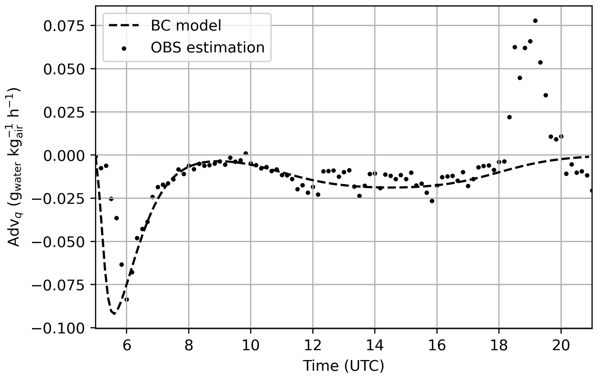
As mentioned in the paper, advection was estimated with measurements of wind, temperature and specific humidity from an atmospheric weather station network operated by the Servei Meteorològic of Catalunya. More details on how the advection was calculated can be found in Sect. 4.2 “Mixed layer data: Model initialization & advection” and in Appendix B of the article by Mangan et al. (2023a). The unique differences between the cited article and the present study are that we used the daily advection estimation of 17 July 2021 instead of the monthly average and that we smoothed the advection term by fitting the estimations to a continuous function. We smoothed the estimated advection to ensure that the temporal evolution of the environmental variables would be differentiable. This was desired to facilitate the interpretation of the tendency terms. The continuous function we used was
where Y=θ and q and i represent the different advection regimes. In our case there were two regimes: (1) the warm and very dry regime from 05:00 to 08:00 UTC and (2) the very warm and slightly dry regime from 09:00 to 18:00 UTC. Coefficients AY,i, tini,i, tfin,i, , and represent the amplitude of the advection, the initial and final time when advection occurs, and the rate of change from no advection to advection and vice versa. Note that the sea breeze (advection of cold and wet air from 18:00 UTC onwards) was not imposed as a boundary condition in the simulations because at this time the atmosphere was not well mixed and therefore we did not study that period. However, the smooth function of the sea breeze advection was also calculated for the temperature (not shown here), as it was imposed for the TEM-ADV experiment.
The estimations of heat and moisture advection together with the smoothed advection terms used as boundary conditions in the control experiment are shown in Figs. A1 and A2.
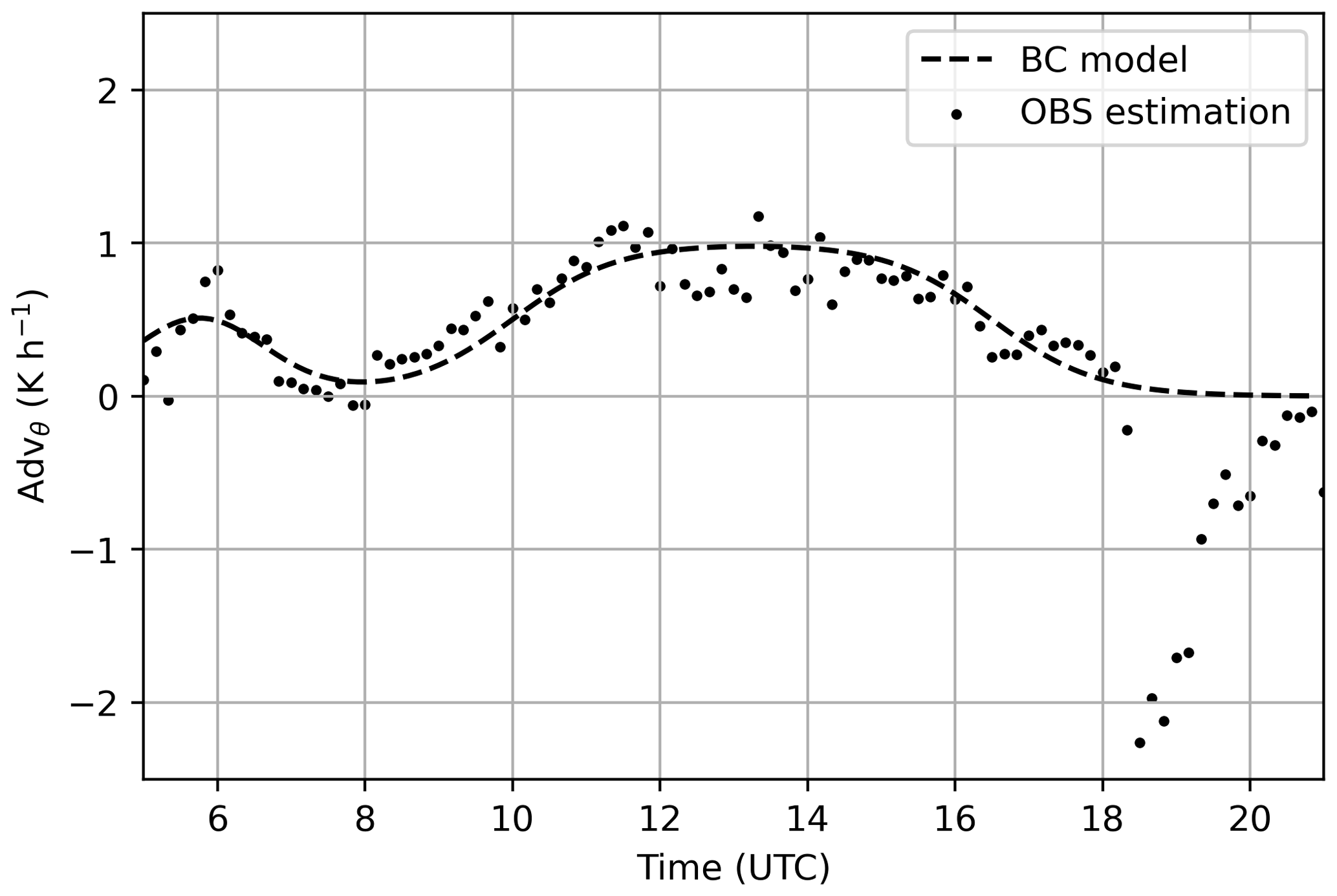
Figure A1Temporal evolution of the temperature advection. Black dots indicate the estimations from the network of atmospheric weather stations and the dashed line shows the smoothed advection of temperature that was added as a boundary condition to the control experiment.
A2 Leaf level: photosynthesis response curves
Figures A3a and A3b show the observed and modeled net CO2 assimilation curves to Ci and PAR.
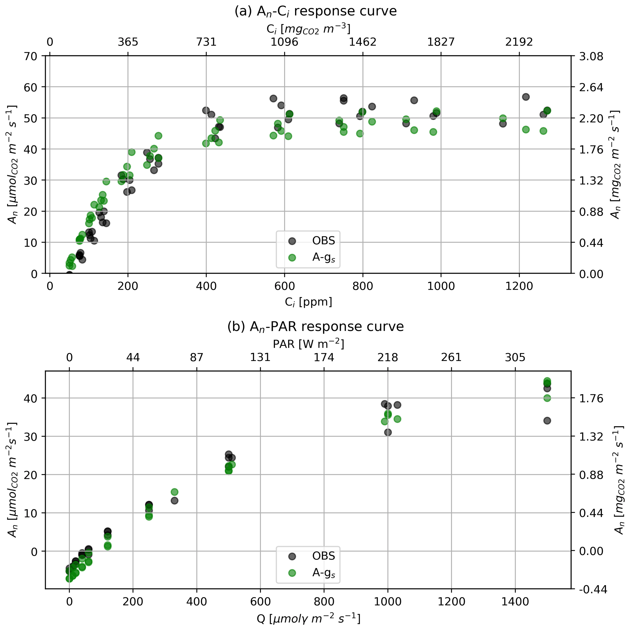
Figure A3Response curves of net CO2 assimilation rate to (a) Ci and (b) PAR or molar flux of photons (Q). Black dots are the observations and green dots are the A-gs modeled results. A-gs predictions were made using the environmental conditions set in the leaf chamber (same temperature, radiation, and CO2 concentration) and the optimized parameters shown in Table 3.
A3 Leaf level: procedure to calculate net CO2 assimilation rate and leaf transpiration
In this section we detail how we estimated the net assimilation rate and leaf transpiration based on observations. We have called these estimations “post-processed observations” because they combine observations of the closed chamber portable photosynthesis system (LiCOR 6400-XT) and of the in-canopy and above-canopy sensors of T, PAR, specific humidity, and Ca. Although the post-processed observations are not direct observations and they have certain limitations due to the assumptions made, we used them as a way of visualizing the essential diurnal variability of leaf fluxes. To study the leaf gas exchange in greater detail, another procedure should be used in combination. We do so by complementing the observations with models of the leaf gas exchange. The net assimilation rate and the leaf transpiration have been calculated using the following equations:
where μ is the ratio of molecular diffusivities of water vapor and CO2, mair is the molecular mass of air, is the molecular mass of water, and RH is the relative humidity of the air. T, RH, and Ca were taken from sensors inside the canopy (T and RH at 0.105 m) and above the canopy (Ca at 3 m). Ci was calculated using the ratio of internal to external CO2 concentration measured inside the closed chamber portable photosynthesis system (LiCOR 6400-XT) and the Ca measured above the canopy.
LIAISE observations are available in the following database: https://liaise.aeris-data.fr/products/ (Boone et al., 2023). Any other data needed to replicate this research will be made available on request.
The supplement related to this article is available online at: https://doi.org/10.5194/bg-21-2425-2024-supplement.
RGA carried out the numerical experiment and the corresponding analyses. JVGdA, HdB, and RGA developed the ideas that led to the study and discussed the results thoroughly. RGA developed and calculated the tendency equations. HdB provided his expertise in the leaf gas exchange measurements and plant physiology, and he organized the leaf measurement plan for La Cendrosa in the LIAISE field campaign, also providing the necessary equipment. MRM and OH were in charge of the surface energy balance station at La Cendrosa, and they also developed an initial CLASS simulation for the location, which was then adapted for the current study. They also provided valuable discussions which shaped the research presented here. All authors read and approved the manuscript.
The contact author has declared that none of the authors has any competing interests.
Publisher’s note: Copernicus Publications remains neutral with regard to jurisdictional claims made in the text, published maps, institutional affiliations, or any other geographical representation in this paper. While Copernicus Publications makes every effort to include appropriate place names, the final responsibility lies with the authors.
The authors are grateful to the organizers, hosts, and participants of the LIAISE campaign because thanks to them the development of this research was possible. In particular, we would like to acknowledge Martin Best, Joaquim Bellvert, Jennifer Brooke, Jan Polcher, and Pere Quintana for their work on the LIAISE steering committee, and Henk Snellen, Getachew Adnew, Marc Castellnou, Siluo Chen, Kevin van Diepen, Siluo Chen, Kim Faassen, Wouter Mol, Robbert Moonen, Ruben Schulte, and Gijs Vis for their work on the LIAISE Dutch team during the experiment. We would also like to reiterate our gratitude to Kevin van Diepen, Siluo Chen, and Kim Faassen for contributing to the measurements of the leaf gas exchange during the LIAISE field campaign.
This research has been supported by the Dutch Research Council under the project Cloud-Roots – Clouds rooted in a heterogeneous biosphere (project no. OCENW.KLEIN.407).
This paper was edited by Andreas Ibrom and reviewed by two anonymous referees.
Ball, J. T., Woodrow, I. E., and Berry, J. A.: A model predicting stomatal conductance and its contribution to the control of photosynthesis under different environmental conditions, in: Progress in photosynthesis research: volume 4 proceedings of the VIIth international congress on photosynthesis providence, Rhode Island, USA, august 10–15, 1986, 221–224, Springer, https://doi.org/10.1007/978-94-017-0519-6_48, 1987. a
Best, M. J., Abramowitz, G., Johnson, H. R., Pitman, A. J., Balsamo, G., Boone, A., Cuntz. M., Decharme, B., Dirmeyer, P. A., Dong, J., Ek, M., Guo, Z., Haverd, V., van den Hurk, B. J. J., Nearing, G. S., Pak, B., Peters-Lidard, C., Santanello JR., J. A., Stevens, L., and Vuichard, N.: The plumbing of land surface models: benchmarking model performance, J. Hydrometeorol., 16, 1425–1442, https://doi.org/10.1175/JHM-D-14-0158.1, 2015. a
Bonan, G. B., Patton, E. G., Finnigan, J. J., Baldocchi, D. D., and Harman, I. N.: Moving beyond the incorrect but useful paradigm: reevaluating big-leaf and multilayer plant canopies to model biosphere-atmosphere fluxes–a review, Agr. Forest Meteorol., 306, 108435, https://doi.org/10.1016/j.agrformet.2021.108435, 2021. a, b
Boone, A. A.: Land surface Interactions with the Atmosphere over the Iberian Semi-arid Environment (LIAISE), Gewex News, HAL Id: hal-02392949, 2019. a
Boone, A., Bellvert, J., Best, M., Brooke, J., Canut-Rocafort, G., Cuxart, J., Hartogensis, O., Le Moigne, P., Miró, J. R., Polcher, J., Price, J., Quintana-Seguí, P., and Wooster, M.: Updates on the international land surface interactions with the atmosphere over the Iberian semi-arid environment (LIAISE) field campaign, Gewex News, HAL Id: hal-03842003, 2021. a, b
Boone, A. A., Bellvert, J., Best, M., Brooke, J., Canut-Rocafort, G., Cuxart, J., Hartogensis, O., Le Moigne, P., Ramon-Miró, J., Polcher, J., Price, J., Quintana-Seguí, P., and Wooster, M.: LIAISE Field Campaign dataset, Aeris Data, https://liaise.aeris-data.fr/products/ (last access: 13 May 2024), 2023. a
Boussetta, S., Balsamo, G., Beljaars, A., Panareda, A.-A., Calvet, J.-C., Jacobs, C., van den Hurk, B., Viterbo, P., Lafont, S., Dutra, E., Jarlan, L., Balzarolo, M., Papale, D., and van der Werf, G.: Natural land carbon dioxide exchanges in the ECMWF integrated forecasting system: Implementation and offline validation, J. Geophys. Res.-Atmos., 118, 5923–5946, 2013. a
Calvet, J.-C., Noilhan, J., Roujean, J.-L., Bessemoulin, P., Cabelguenne, M., Olioso, A., and Wigneron, J.-P.: An interactive vegetation SVAT model tested against data from six contrasting sites, Agr. Forest Meteorol., 92, 73–95, 1998. a
Casso-Torralba, P., Vilà-Guerau de Arellano, J., Bosveld, F., Soler, M. R., Vermeulen, A., Werner, C., and Moors, E.: Diurnal and vertical variability of the sensible heat and carbon dioxide budgets in the atmospheric surface layer, J. Geophys. Res.-Atmos., 113, https://doi.org/10.1029/2007JD009583, 2008. a
Chen, T. H., Henderson-Sellers, A., Milly, P. C. D., Pitman, A. J., Beljaars, A. C. M., Polcher, J., Abramopoulos, F., Boone, A. A., Chang, S., Chen, F., Dai, Y., Desborough, C. E., Dickinson, R. E., Dümenil, L., Ek, M., Garratt, J. R., Gedney, N., Gusev, Y. M., Kim, J., Koster, R., Kowalczyk, E. A., Laval, K., Lean, J., Lettenmaier, D., Liang, X., Mahfouf, J.-F., Mengelkamp, H.-T., Mitchell, K., Nasonova, O. N., Noilhan, J., Robock, A., Rosenzweig, C., Schaake, J., Schlosser, C. A., Schulz, J.-P., Shao, Y., Shmakin, A. B., Verseghy, D. L., Wetzel, P., Wood, E. F., Xue, Y., Yang, Z.-L., and Zeng, Q.: Cabauw experimental results from the project for intercomparison of land-surface parameterization schemes, J. Climate, 10, 1194–1215, 1997. a
Collatz, G. J., Ball, J. T., Grivet, C., and Berry, J. A.: Physiological and environmental regulation of stomatal conductance, photosynthesis and transpiration: a model that includes a laminar boundary layer, Agr. Forest Meteorol., 54, 107–136, 1991. a
Combe, M., de Arellano, J. V.-G., Ouwersloot, H. G., and Peters, W.: Plant water-stress parameterization determines the strength of land–atmosphere coupling, Agr. Forest Meteorol., 217, 61–73, 2016. a, b
Doutriaux-Boucher, M., Webb, M., Gregory, J. M., and Boucher, O.: Carbon dioxide induced stomatal closure increases radiative forcing via a rapid reduction in low cloud, Geophys. Res. Lett., 36, https://doi.org/10.1029/2008GL036273, 2009. a
Echer, F. R. and Rosolem, C. A.: Cotton leaf gas exchange responses to irradiance and leaf aging, Biol. Plantarum, 59, 366–372, 2015. a
Farquhar, G. D., von Caemmerer, S. V., and Berry, J. A.: A biochemical model of photosynthetic CO2 assimilation in leaves of C 3 species, Planta, 149, 78–90, 1980. a
Goudriaan, J., Van Laar, H., Van Keulen, H., and Louwerse, W.: Photosynthesis, CO2 and plant production, Wheat Growth and Modelling, NATO ASI Science, vol 86. Springer, Boston, MA, 107–122, https://doi.org/10.1007/978-1-4899-3665-3_10, 1985. a, b, c, d
Helbig, M., Gerken, T., Beamesderfer, E. R., Baldocchi, D. D., Banerjee, T., Biraud, S. C., Brown, W. O. J., Brunsell, N. A., Burakowski, E. A., Burns, S. P., Butterworth, B. J., Chan, W. S., Davis, K. J., Desai, A. R., Fuentes, J. D., Hollinger, D. Y., Kljun, N., Mauder, M., Novick, K. A., Perkins, J. M., Rahn, D. A., Rey-Sánchez, C., Santanello, J. A., Scott, R. L., Seyednasrollah, B., Stoy, P. C., Sullivan, R. C., Vilà-Guerau de Arellano, J., Wharton, S., Yi, C., and Richardson, A. D.: Integrating continuous atmospheric boundary layer and tower-based flux measurements to advance understanding of land-atmosphere interactions, Agr. Forest Meteorol., 307, 108509, https://doi.org/10.1016/j.agrformet.2021.108509, 2021. a
Henderson-Sellers, A., Pitman, A., Love, P., Irannejad, P., and Chen, T.: The project for intercomparison of land surface parameterization schemes (PILPS): Phases 2 and 3, B. Am. Meteor. Soc., 76, 489–504, 1995. a
Holtslag, A., Svensson, G., Baas, P., Basu, S., Beare, B., Beljaars, A., Bosveld, F., Cuxart, J., Lindvall, J., Steeneveld, G., Tjernström, M., and van de Wiel, B. J. H.: Stable atmospheric boundary layers and diurnal cycles: challenges for weather and climate models, B. Am. Meteor. Soc., 94, 1691–1706, 2013. a
Jacobs, C. M. and de Bruin, H. A.: Predicting regional transpiration at elevated atmospheric CO2: influence of the PBL–vegetation interaction, J. Appl. Meteor. Clim., 36, 1663–1675, 1997. a
Jacobs, C. M. J.: Direct impact of atmospheric CO2 enrichment on regional transpiration, Wageningen University and Research, 24801, https://edepot.wur.nl/206972 (last access: 21 May 2024), 1994. a, b, c
Jarvis, P. G. and McNaughton, K.: Stomatal control of transpiration: scaling up from leaf to region, in: Advances in ecological research, 15, 1–49, Elsevier, https://doi.org/10.1016/S0065-2504(08)60119-1, 1986. a, b, c
Kaimal, J. C. and Finnigan, J. J.: Atmospheric boundary layer flows: their structure and measurement, Oxford University Press, https://doi.org/10.1093/oso/9780195062397.001.0001, 1994. a
Kivalov, S. N. and Fitzjarrald, D. R.: Quantifying and modelling the effect of cloud shadows on the surface irradiance at tropical and midlatitude forests, Boundary-Lay. Meteorol., 166, 165–198, 2018. a
Knohl, A. and Baldocchi, D. D.: Effects of diffuse radiation on canopy gas exchange processes in a forest ecosystem, J. Geophys. Res.-Biogeo., 113, https://doi.org/10.1029/2007JG000663, 2008. a
Mangan, M. R., Hartogensis, O., Boone, A., Branch, O., Canut, G., Cuxart, J., de Boer, H. J., Le Page, M., Martínez-Villagrasa, D., Miró, J. R., Price, J., and Vilà-Guerau de Arellano, J.: The surface-boundary layer connection across spatial scales of irrigation-driven thermal heterogeneity: An integrated data and modeling study of the LIAISE field campaign, Agr. Forest Meteorol., 335, 109452, https://doi.org/10.1016/j.agrformet.2023.109452, 2023a. a, b, c, d, e, f, g, h
Mangan, M. R., Hartogensis, O., van Heerwaarden, C., and Vilà-Guerau de Arellano, J.: Evapotranspiration controls across spatial scales of heterogeneity, Q. J. Roy. Meteor. Soc., 149, 2696–2718, 2023b. a
Masson, V., Le Moigne, P., Martin, E., Faroux, S., Alias, A., Alkama, R., Belamari, S., Barbu, A., Boone, A., Bouyssel, F., Brousseau, P., Brun, E., Calvet, J.-C., Carrer, D., Decharme, B., Delire, C., Donier, S., Essaouini, K., Gibelin, A.-L., Giordani, H., Habets, F., Jidane, M., Kerdraon, G., Kourzeneva, E., Lafaysse, M., Lafont, S., Lebeaupin Brossier, C., Lemonsu, A., Mahfouf, J.-F., Marguinaud, P., Mokhtari, M., Morin, S., Pigeon, G., Salgado, R., Seity, Y., Taillefer, F., Tanguy, G., Tulet, P., Vincendon, B., Vionnet, V., and Voldoire, A.: The SURFEXv7.2 land and ocean surface platform for coupled or offline simulation of earth surface variables and fluxes, Geosci. Model Dev., 6, 929–960, https://doi.org/10.5194/gmd-6-929-2013, 2013. a
Mol, W. B., van Stratum, B. J., Knap, W. H., and van Heerwaarden, C. C.: Reconciling observations of solar irradiance variability with cloud size distributions, J. Geophys. Res.-Atmos., 128, e2022JD037894, https://doi.org/10.1029/2022JD037894, 2023. a, b, c
Monin, Andre\ĭ, S. and Obukhov, A. M.: Basic laws of turbulent mixing in the surface layer of the atmosphere, Contrib. Geophys. Inst. Acad. Sci. USSR, 151, e187, 1954. a
Niyogi, D., Chang, H.-I., Saxena, V., Holt, T., Alapaty, K., Booker, F., Chen, F., Davis, K. J., Holben, B., Matsui, T., Meyers, T., Oechel, W. C., Pielke Sr., R. A., Wells, R., Wilson, K., and Xue, Y.: Direct observations of the effects of aerosol loading on net ecosystem CO2 exchanges over different landscapes, Geophys. Res. Lett., 31, https://doi.org/10.1029/2004GL020915, 2004. a, b, c
Noilhan, J. and Planton, S.: A simple parameterization of land surface processes for meteorological models, Mon. Weather Rev., 117, 536–549, 1989. a
Pedruzo-Bagazgoitia, X., Ouwersloot, H., Sikma, M., Van Heerwaarden, C., Jacobs, C., and Vilà-Guerau de Arellano, J.: Direct and diffuse radiation in the shallow cumulus–vegetation system: Enhanced and decreased evapotranspiration regimes, J. Hydrometeorol., 18, 1731–1748, 2017. a, b, c, d, e, f
Pedruzo-Bagazgoitia, X., Patton, E., Moene, A., Ouwersloot, H., Gerken, T., Machado, L., Martin, S., Sörgel, M., Stoy, P., Yamasoe, M., and Vilà-Guerau de Arellano, J.: Investigating the Diurnal Radiative, Turbulent, and Biophysical Processes in the Amazonian Canopy-Atmosphere Interface by Combining LES Simulations and Observations, J. Adv. Model. Earth Sy., 15, e2022MS003210, https://doi.org/10.1029/2022MS003210, 2023. a
Renner, M., Brenner, C., Mallick, K., Wizemann, H.-D., Conte, L., Trebs, I., Wei, J., Wulfmeyer, V., Schulz, K., and Kleidon, A.: Using phase lags to evaluate model biases in simulating the diurnal cycle of evapotranspiration: a case study in Luxembourg, Hydrol. Earth Syst. Sci., 23, 515–535, https://doi.org/10.5194/hess-23-515-2019, 2019. a
Renner, M., Kleidon, A., Clark, M., Nijssen, B., Heidkamp, M., Best, M., and Abramowitz, G.: How well can land-surface models represent the diurnal cycle of turbulent heat fluxes?, J. Hydrometeorol., 22, 77–94, 2021. a, b, c
Restrepo-Coupe, N., Levine, N. M., Christoffersen, B. O., Albert, L. P., Wu, J., Costa, M. H., Galbraith, D., Imbuzeiro, H., Martins, G., da Araujo, A. C., Malhi, Y. S., Zeng, X., Moorcroft, P., and Saleska, S. R.: Do dynamic global vegetation models capture the seasonality of carbon fluxes in the Amazon basin? A data-model intercomparison, Glob. Change Biol., 23, 191–208, 2017. a
Ronda, R., De Bruin, H., and Holtslag, A.: Representation of the canopy conductance in modeling the surface energy budget for low vegetation, J. Appl. Meteorol. Clim., 40, 1431–1444, 2001. a, b, c
Séférian, R., Delire, C., Decharme, B., Voldoire, A., Salas y Melia, D., Chevallier, M., Saint-Martin, D., Aumont, O., Calvet, J.-C., Carrer, D., Douville, H., Franchistéguy, L., Joetzjer, E., and Sénési, S.: Development and evaluation of CNRM Earth system model – CNRM-ESM1, Geosci. Model Dev., 9, 1423–1453, https://doi.org/10.5194/gmd-9-1423-2016, 2016. a
Sellers, P., Randall, D., Collatz, G., Berry, J., Field, C., Dazlich, D., Zhang, C., Collelo, G., and Bounoua, L.: A revised land surface parameterization (SiB2) for atmospheric GCMs. Part I: Model formulation, J. Climate, 9, 676–705, 1996. a
Sikma, M., Ouwersloot, H., Pedruzo-Bagazgoitia, X., Van Heerwaarden, C., and de Arellano, J. V.-G.: Interactions between vegetation, atmospheric turbulence and clouds under a wide range of background wind conditions, Agr. Forest Meteorol., 255, 31–43, 2018. a
Stull, R. B.: An introduction to boundary layer meteorology, vol. 13, Springer Science & Business Media, ISBN 978-90-277-2769-5, 1988. a
Tolk, J. A., Evett, S. R., and Howell, T. A.: Advection influences on evapotranspiration of alfalfa in a semiarid climate, Agron. J., 98, 1646–1654, 2006. a
van Diepen, K., Goudriaan, J., Vilà-guerau De Arellano, J., and De Boer, H.: Comparison of C3 Photosynthetic Responses to Light and CO2 Predicted by the Leaf Photosynthesis Models of Farquhar et al.(1980) and Goudriaan et al.(1985), J. Adv. Model. Earth Sy., 14, e2021MS002976, https://doi.org/10.1029/2021MS002976, 2022. a
van Heerwaarden, C. C., Vilà-Guerau de Arellano, J., Moene, A. F., and Holtslag, A. A.: Interactions between dry-air entrainment, surface evaporation and convective boundary-layer development, Quarterly Journal of the Royal Meteorological Society: A journal of the atmospheric sciences, Applied Meteorology and Physical Oceanography, 135, 1277–1291, 2009. a, b, c, d
van Heerwaarden, C. C., de Arellano, J. V.-G., Gounou, A., Guichard, F., and Couvreux, F.: Understanding the daily cycle of evapotranspiration: A method to quantify the influence of forcings and feedbacks, J. Hydrometeorol., 11, 1405–1422, 2010. a, b, c, d, e
Vico, G., Manzoni, S., Palmroth, S., and Katul, G.: Effects of stomatal delays on the economics of leaf gas exchange under intermittent light regimes, New Phytol., 192, 640–652, 2011. a
Vilà-Guerau de Arellano, J., Ouwersloot, H. G., Baldocchi, D., and Jacobs, C. M.: Shallow cumulus rooted in photosynthesis, Geophys. Res. Lett., 41, 1796–1802, 2014. a
Vilà-Guerau de Arellano, J., Van Heerwaarden, C., Van Stratum, B., and Van Den Dries, K.: Atmospheric boundary layer: Integrating air chemistry and land interactions, Cambridge University Press, https://doi.org/10.1017/CBO9781316117422, 2015. a, b, c, d, e, f
Vilà-Guerau de Arellano, J., Ney, P., Hartogensis, O., de Boer, H., van Diepen, K., Emin, D., de Groot, G., Klosterhalfen, A., Langensiepen, M., Matveeva, M., Miranda-García, G., Moene, A. F., Rascher, U., Röckmann, T., Adnew, G., Brüggemann, N., Rothfuss, Y., and Graf, A.: CloudRoots: integration of advanced instrumental techniques and process modelling of sub-hourly and sub-kilometre land–atmosphere interactions, Biogeosciences, 17, 4375–4404, https://doi.org/10.5194/bg-17-4375-2020, 2020. a
Vilà-Guerau de Arellano, J., Hartogensis, O., Benedict, I., de Boer, H., Bosman, P. J. M., Botía, S., Cecchini, M. A., Fassen, K. A. P., González-Armas, R., van Diepen, K., Heusinkveld, B. G., Janssens, M., Lobos-Roco, F., Luijkx, I. T., Machado, L. A. T., Mangan, M. R., Moene, A. F., Mol, W. B., van der Molen, M., Moonen, R., Ouwersloot, H. G., Park, S.-W., Pedruzo-Bagazgoitia, X., Röckmann, T., Adnew, G. A., Ronda, R., Sikma, M., Schulte, R., van Stratum, B. J. H., Veerman, M. A., van Zanten, M. C., van Heerwaarden, C. C.: Advancing understanding of land–atmosphere interactions by breaking discipline and scale barriers, Ann. NY Acad. Sci., 2023. a