The effect of temperature on photosystem II efficiency across plant functional types and climate

Modeling terrestrial gross primary productivity (GPP) is central to predicting the global carbon cycle. Much interest has been focused on the environmentally induced dynamics of photosystem energy partitioning and how improvements in the description of such dynamics assist the prediction of light reactions of photosynthesis and therefore GPP. The maximum quantum yield of photosystem II (Φ_PSIImax) is a key parameter of the light reactions that influence the electron transport rate needed for supporting the biochemical reactions of photosynthesis. Φ_PSIImax is generally treated as a constant in biochemical photosynthetic models even though a constant Φ_PSIImax is expected only for non-stressed plants. We synthesized reported Φ_PSIImax values from pulse-amplitude-modulated fluorometry measurements in response to variable temperatures across the globe. We found that Φ_PSIImax is strongly affected by prevailing temperature regimes with declined values in both hot and cold conditions. To understand the spatiotemporal variability in Φ_PSIImax, we analyzed the temperature effect on Φ_PSIImax across plant functional type (PFT) and habitat climatology. The analysis showed that temperature's impact on Φ_PSIImax is shaped more by climate than by PFT for plants with broad latitudinal distributions or in regions with extreme temperature variability. There is a trade-off between the temperature range within which Φ_PSIImax remains maximal and the overall rate of decline of Φ_PSIImax outside the temperature range such that species cannot be simultaneously tolerant and resilient to extreme temperatures. Our study points to a quantitative approach for improving electron transport and photosynthetic productivity modeling under changing climates at regional and global scales.

1 Introduction

Plant photosynthesis is central to the carbon cycle (Friedlingstein et al., 2020, 2022). Illuminating its complexity is needed to understand the carbon-cycle–climate feedback and assess food production, biodiversity, and global ecosystem health. Anthropogenic activities have induced a variety of rapid shifts in the earth's climate (IPCC, 2021) that impact photosynthesis and ecosystem services globally (Hatfield et al., 2020; Heinze et al., 2019). Factors such as temperature stress impact photosynthetic carbon assimilation differently across species and climates and have contributed to significant variability in terrestrial ecosystem productivity and carbon sequestration potential (Wahid et al., 2007; Ashraf and Harris, 2013; Heskel et al., 2016; Perez and Feeley, 2020; Kelly et al., 2021). Terrestrial biosphere models (TBMs) have examined and incorporated many mechanisms of stress-induced photoinhibition of vegetation carbon assimilation (Berry and Bjorkman, 1980; Farquhar et al., 1980; Ball et al., 1987; Franks et al., 2017; Lawrence et al., 2019; Parazoo et al., 2020; Yin et al., 2021; Porcar-Castell et al., 2021). However, the inconsistency between physiological process-based modeled gross primary productivity (GPP) and inferred values via satellite and eddy-covariance flux towers continues to be an ongoing challenge (Dietze, 2014; Sun et al., 2019; Zhang and Ye, 2021).

Photosynthesis is typically separated into light-dependent reactions, which involve the absorption of light within the photosystem complexes (photophysical) and its conversion to oxidative and reductive energy (photochemical), and carbon reactions that further utilize the photochemical energy as preserved in energy currency adenosine triphosphate (ATP) and reducing power nicotinamide adenine dinucleotide phosphate (NADPH) to perform carbon fixation through the Calvin–Benson cycle (biochemical) (Whatley et al., 1963; Kamen, 1963; Stirbet et al., 2019; Buchanan, 2016). Process-based models of net photosynthetic CO₂ assimilation generally center on the simulation of the biochemical reactions that are coupled with gas exchange via stomata (Farquhar et al., 1980; Ball et al., 1987; Lin et al., 2012; Yin et al., 2021). These models implement temperature regulation on biochemical kinetics (Rogers et al., 2017) and environmental dependence of stomatal conductance (Buckley, 2017), allowing mechanistic descriptions of the impact of water, temperature, and CO₂ concentrations on the dynamics of biochemical reactions. However, light reactions, especially mechanistic regulation by environmental factors, are treated less extensively.

Photophysical reactions control the dissipation of absorbed energy among different pathways, including fluorescence, photochemistry (PQ), constitutive heat dissipation, and non-photochemical quenching (NPQ). These pathways are subject to the constraint of energy conservation. NPQ can be further separated into energy-dependent and energy-independent mechanisms. The energy-dependent NPQ, also known as reversible NPQ, quickly relaxes after removing illumination and is connected to the xanthophyll cycle (Johnson et al., 1993; Demmig-Adams and Adams, 2006). The energy-independent NPQ, also known as sustained NPQ, relaxes at longer timescales and can operate seasonally or even inter-annually with the mitigation of environmental stresses (e.g., temperature, water), and it involves protein accumulation and photoinhibition (Demmig-Adams and Adams, 2006; Takahashi and Badger, 2011; Tietz et al., 2017). The PQ pathway transports electrons and protons to produce NADPH and ATP, consequently regulating the carbon reaction rates of photosynthesis. This pathway is typically quantified by the fraction of available photosystem II (PSII) reaction centers (qL) for charge separation after receiving excitation energy. When the NPQ pathway is completely disengaged (NPQ = 0) and all PSII reaction centers are open (qL = 1) under non-stress conditions, plants operate with maximum light use efficiency (LUE) for biochemical carbon assimilation, with an idealized maximum quantum yield of photosystem II (Φ_PSIImax) of 0.75–0.85 (Kitajima and Butler, 1975; Bjorkman and Demmig, 1987; Genty et al., 1989; Corcuera et al., 2011). This value is generally treated as an environmentally independent constant in photosynthesis models (e.g., 0.85 in the Community Land Model; Lawrence et al., 2019).

However, Φ_PSIImax can be irreversibly downregulated due to plant energy-independent NPQ response to temperature and other environmental stresses, especially extreme temperature, or as a result of photodamage to reaction centers (i.e., qL is less than 1 even when plants are fully dark-adapted; Porcar-Castell, 2011). This downregulation can induce a significant reduction in vegetation productivity (Havaux, 1991; Oberhuber and Edwards, 1993; Lu and Zhang, 1999; Murata et al., 2007; Ferguson et al., 2020; Kunert et al., 2022) but has not been mechanistically parameterized in most photosynthesis models. Moreover, this impact of stress on the light reactions has been found to be highly variable among plant species across diverse regions (Li et al., 2008; Corcuera et al., 2011; Marias et al., 2016; Perez and Feeley, 2020). In the Amazon, extreme temperature-induced reduction in Φ_PSIImax is irreversible and currently decreasing the productivity of tropical forests, with large variability in response among forest species (Tiwari et al., 2021). In addition, distinct differences in temperature tolerance and resilience of Φ_PSIImax values are also found among the same species growing in different habitats (Corcuera et al., 2011; Fadrique et al., 2022). To better assess the tolerance and resilience of plant photosynthesis to more extreme climate change, there is an urgent need for a more mechanistic understanding and parameterization of the environments' impact on photosystem efficiency and its variability across species and habitats (McCallum et al., 2013; Dusenge et al., 2019; Fadrique et al., 2022).

The most common method for determining the various quantum yields of energy dissipation pathways is via monitoring chlorophyll a fluorescence (ChlaF). Pulse-amplitude-modulated (PAM) fluorometry is a routine non-invasive method for investigating energy partitioning among the four dissipation pathways (Kitajima and Butler, 1975; Bjorkman and Demmig, 1987; Klughammer and Schreiber, 2008; Porcar-Castell, 2011; Lazár, 2015) and can serve as a bridge to modeling mechanistic partitioning of adsorbed light energy at the leaf level (Gu et al., 2019; Han et al., 2022). A dark-adapted, homeostatic plant minimizes the energy partitioning to the thermal and non-photochemical dissipation pathways, leading to the maximum light allocation fraction to the photochemical pathway (Klughammer and Schreiber, 2008). PAM fluorometry experiments identify Φ_PSIImax by quantifying the ratio of the increase in fluorescence yield during a saturation pulse (Fv) to the maximal fluorescence yield of a dark-adapted sample (Fm). At the canopy level, ground-based and satellite solar-induced ChlaF (SIF) measurements (Mohammed et al., 2019) have been increasingly integrated or assimilated to facilitate regional and global-scale GPP prediction (Lee et al., 2015; Norton et al., 2018, 2019; Bacour et al., 2019a, b; Yang et al., 2021). The accuracy of this model–SIF data integration depends on the ability of these models to represent GPP–SIF relationships at leaf and canopy levels. Sun et al. (2023a, b) highlighted the complexity of fully describing the many leaf- and canopy-level factors at play in the GPP–SIF relationship. Parazoo et al. (2020) examined seven TBMs that included SIF-based photosynthetic parameterization and found that much of their discrepancy may be tied, among other things, to the need for better descriptions of leaf mechanisms of energy partitioning under environmental stress; others have pointed out similar areas of needed research (Rogers et al., 2017; Kumarathunge et al., 2019).

Our previous effort (Gu et al., 2019) has modeled the leaf-level GPP–SIF dynamics as a function of NPQ, qL, Φ_PSIImax, and absorbed photosynthetically active radiation (APAR). That study pointed out a need for mechanistic descriptions of how NPQ, qL, and Φ_PSIImax respond to environmental conditions to accurately predict environmental regulation of the GPP–SIF relationship at the leaf level. By empirically fitting the NPQ rate coefficient with a function of relative light saturation and combining it with the biochemical-reaction-centered photosynthesis model, van der Tol (2014) estimated the responses of leaf-level fluorescence yield to changing temperature, light, and CO₂ concentration, indicating that quantifying environmental responses of photochemical yield are a key step in addressing the integrated environmental impacts on GPP–SIF dynamics. Therefore, here we present a novel model of Φ_PSIImax response to temperature variation by collecting and applying a global-scale database of published PAM measurements, with an emphasis on parameterizing the different temperature tolerance and resilience of various plant functional types (PFTs) and investigating how habitat climatology may affect this temperature–Φ_PSIImax relationship. This study will deliver the first global-scale quantification of temperature impact on photosystem II efficiency and its variability across PFTs and habitat climatology and build a theoretical basis for assessing vegetation light utilization potential for carbon sequestration under climate change and climate extremes. Modeling temperature regulation on Φ_PSIImax is important for assessing extreme temperature impacts on the maximum electron transport rate (J_max) in biochemical-reaction-centered photosynthesis models. Moreover, characterizing the temperature response of Φ_PSIImax will allow us to connect other light partitioning mechanisms to temperature change, building the first step of resolving coupled SIF and GPP responses to temperature change. With the support of the temperature dependence modeling of Φ_PSIImax provided by this study, a full modeling of temperature responses of photosynthetic variables, including qL, NPQ, and Φ_F, can be achieved by coupling the photophysical reactions (Gu et al., 2019), photochemical reactions (Gu et al., 2023), and the Farquhar biochemical model (Farquhar et al., 1980).

In this study, we developed specific temperature response functions of Φ_PSIImax for 12 plant functional types (PFTs) commonly used in TBMs and determined temperature “tolerance” and “resilience” parameters for Φ_PSIImax. In addition, the climatological impacts on the temperature tolerance and resilience of Φ_PSIImax are also examined via creating a climatology index and incorporating it into the original parameterization. Finally, we identified specific geographical locations where climate significantly affects PFT-specific temperature–Φ_PSIImax relationships.

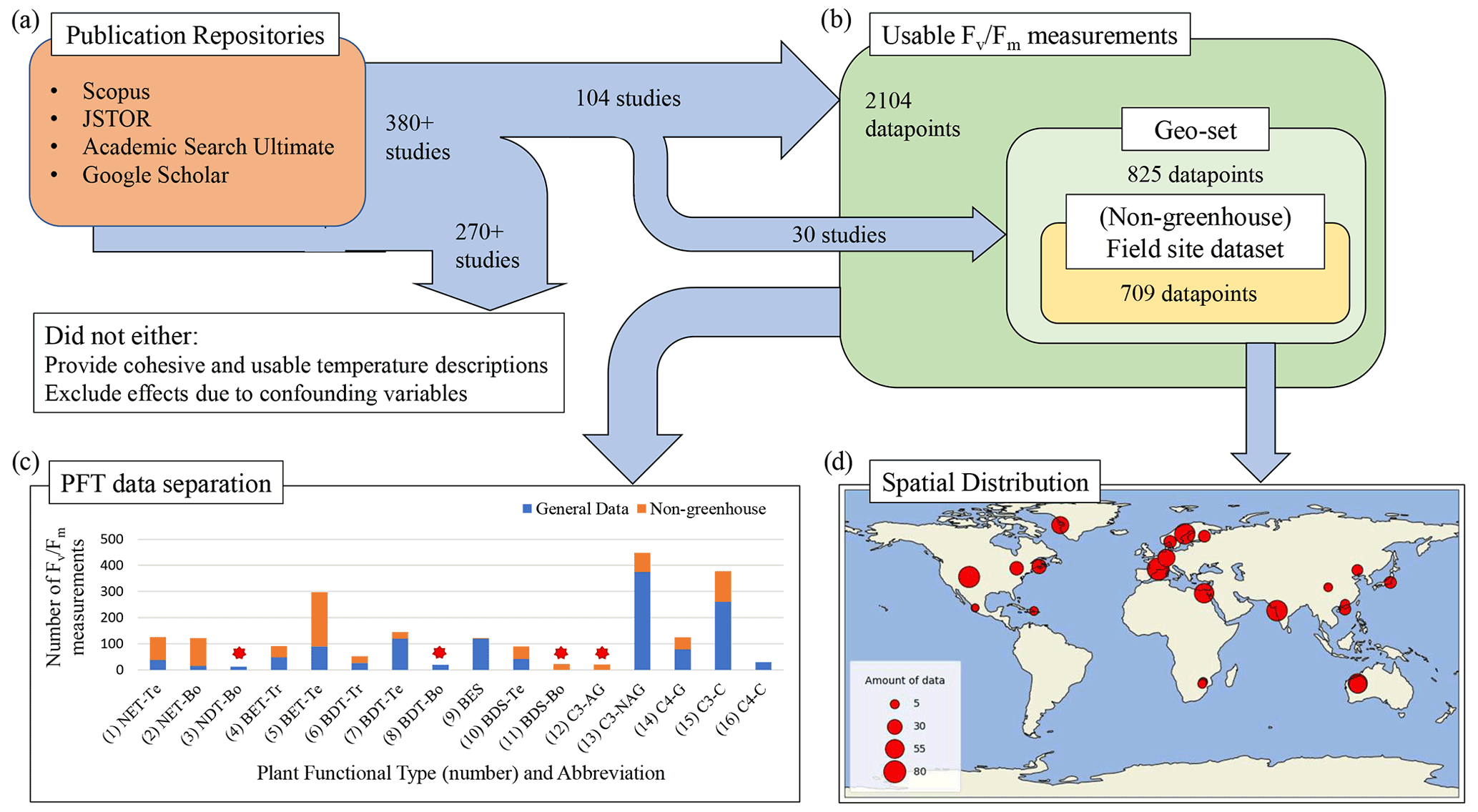
Figure 1 Data acquisition, selection, and composition pipeline. (a) A summary of the rule-specific procedure of mining and selecting PAM fluorometry data from publication repositories. (b) The definition of sub-datasets according to the availability of geographic information for the data and PAM experimental methodology. (c) The number of available PAM data for the 16 chosen PFTs, being (1) needleleaf evergreen temperate tree (NET-Te), (2) needleleaf evergreen boreal tree (NET-Bo), (3) needleleaf deciduous boreal tree (NDT-Bo), (4) broadleaf evergreen tropical tree (BET-Tr), (5) broadleaf evergreen temperate tree (BET-Te), (6) broadleaf deciduous tropical tree (BDT-Tr), (7) broadleaf deciduous temperate tree (BDT-Te), (8) broadleaf deciduous boreal tree (BDT-Bo), (9) broadleaf evergreen shrub (BES), (10) broadleaf deciduous temperate shrub (BDS-Te), (11) broadleaf deciduous boreal shrub (BDS-Bo), (12) C3 Arctic grass (C3-AG), (13) C3 non-Arctic grass (C3-NAG), (14) C4 grass (C4-G), (15) C3 crop (C3-C), and (16) C4 crop (C4-C). A PFT that has less than 30 data is marked by a red star. (d) Spatial distribution of the “geo-set” of data and the number of measurements from each study represented by the circle size.

2 Data and methods

2.1 PAM fluorometry data collection

We quantified the impact of temperature on Φ_PSIImax by collecting 380 published studies with Fv$/$Fm data measured using the PAM fluorometry method from four publication repositories (Fig. 1a). To isolate temperature dependence from other external regulators of Φ_PSIImax, we mined and selected data from studies that provided cohesive descriptions of temperature for the relevant measurements and excluded the effects of other confounding variables (e.g., water, nutrient, light stress). Following this data selection strategy, we selected PAM observations from the controlled environments (e.g., greenhouse) where nutrients, lights, and water availability have been optimized and where only varied temperatures are considered. We also included PAM data from field experiments with the description of no other stress conditions except for temperature. Following these guidelines, a total of 104 studies out of the 380 publications were finally selected. Once selected, the measurements of Fv$/$Fm were either directly recorded (for tabular and text reporting of Fv$/$Fm values) or extracted from graphics using a web-based extraction tool (Rohatgi, 2021). The corresponding experimental temperature, the study location, measurement techniques, duration of the temperature exposure, taxonomic description, and other factors of interest were recorded (dataset in Supplement Sect. 1). As reporting of temperature was not consistent across studies, we used three methods to identify experimental temperature: (1) for publications that utilized a diurnal description of temperature, the diurnal mean temperature was used as a proxy measurement temperature, as determined by the average of the minimum and maximum reported values; (2) for studies performed in uncontrolled temperature environments, the mean temperature experienced by the plant during the experiment period was used; and (3) if a study lacked a well-described reporting of specific experimental temperature, the mean temperature during the experimental period was collected from the 0.5° × 0.5° global atmospheric forcing dataset, CRUNCEP v.7 (Viovy, 2018).

In total, 2329 measurements from 104 studies were recorded in the final database, with 2104 measurements meeting the criteria for use in modeling. All measurements included plant taxonomic descriptions, culminating in 146 distinct species from 46 different family groups and 29 orders. We grouped these measurements into 16 PFT-specific sub-datasets (Fig. 1b). These sub-datasets were analyzed for PFT-specific Φ_PSIImax responses to temperature change. In addition, within the 2104 total measurements, a subset of 825 measurements from 30 publications included explicit latitude and longitude information. This “geo-set” of data covers diverse geographic regions across a bounding range of [35.4° S, 107° W, 69.25° N, 140° E] (Fig. 1d). For data within this geo-set, 709 measurements were collected from in-the-wild plants located in natural environments (non-greenhouse) (Fig. 1c). This geo-specific and climate-affected sub-dataset, herein called field site sub-dataset, was used to assess the effects of climatological temperature on the response behavior of plant Φ_PSIImax to temperature change.

2.2 Parameterizing temperature regulation on Φ_PSIImax for each plant functional type

We employ the PFT-specific sub-datasets to parameterize a general temperature response function of Φ_PSIImax for all data, as well as 12 PFT-specific temperature response functions. We quantified the temperature tolerance and resilience of Φ_PSIImax for each PFT based on the corresponding parameterized temperature response function.

2.2.1 Selecting the fitting function and quantifying temperature tolerance and resilience

Features of a function desirable for the parameterization of the gathered data are as follows:

• capturing the characteristics of the temperature response of Φ_PSIImax

• continuity across the full range of temperatures at a global scale

• well-suited for further refinement of parameters with additional data through fitting methods

• physically interpretable parameters.

With these characteristics in mind, the selected parameterization scheme was a rectangular function of temperature with the form

$$\begin{array}{}\text{(1)}& \begin{array}{rl}{\mathrm{\Phi }}_{\text{PSIImax}}& =F_{\mathrm{v}}/F_{\mathrm{m}}=f\left(T\right)\\ & =a{\displaystyle \frac{\mathrm{1}}{\mathrm{2}}}\left(\mathrm{erf}\left({\displaystyle \frac{T-m_{\mathrm{1}}}{s_{\mathrm{1}}}}\right)+\mathrm{erf}\left({\displaystyle \frac{m_{\mathrm{2}}-T}{s_{\mathrm{2}}}}\right)\right),\end{array}\end{array}$$

where T is the temperature in °C and erf is a special class of the sigmoid function called the error function (erf):

$$\begin{array}{}\text{(2)}& \mathrm{erf}\left(z\right)={\displaystyle \frac{\mathrm{2}}{\sqrt{\mathit{\pi }}}}{\int }_{\mathrm{0}}^z{e}^{-t^{\mathrm{2}}}\mathrm{d}t.\end{array}$$

Each of the five parameters has a physical interpretation. The a parameter is the maximal value of Φ_PSIImax under no limitation from temperature or other environmental factors. The m₁ (m₂) parameters mark the temperature at which Φ_PSIImax has declined by 50 % of the a value (also called T₅₀; see Marias et al., 2016; Leon-Garcia and Lasso, 2019; Perez and Feeley, 2020) at cold (hot) temperatures, with the units of °C. The s₁ (s₂) parameters have units of °C and indicate the slope of peak Φ_PSIImax decrease at the m₁ (m₂) temperature values, which can be thought of as a plant's resilience to cold (hot) temperatures, as a smaller s₁ (s₂) means a more rapid decline in Φ_PSIImax under cold (hot) temperatures, indicating a lower resilience to cold (hot) temperatures.

Furthermore, the temperature range within which the predicted Φ_PSIImax remains steady at its maximum (a) can be estimated by creating a linear combination of s_i and m_i parameters (Eqs. 3 and 4) shown below. The lower (T_MC) and upper (T_MH) bounds of this temperature range are referred to as a plant's tolerance to cold and hot temperatures, respectively.

$$\begin{array}{}\text{(3)}& {\displaystyle }& {\displaystyle }{T}_{\text{MC}}=m_{\mathrm{1}}+\mathrm{2}{s}_{\mathrm{1}}\text{(4)}& {\displaystyle }& {\displaystyle }{T}_{\text{MH}}=m_{\mathrm{2}}-\mathrm{2}{s}_{\mathrm{2}}\end{array}$$

Φ_PSIImax starts to decrease from its peak value as the temperature drops below T_MC or heats above T_MH. We determined the best fit for the parameters in Eq. (1) using a variation of the Levenberg–Marquardt method (LMFIT package version 1.0.3) (Newville et al., 2014). The model performance was indicated using the coefficient of determination (R²).

2.2.2 Model fitting and parameter constraints

To ensure that the model could consistently capture the pattern shown in the gathered data, a cross-validation test for parameterizing Eq. (1) was performed. The full dataset of measurements using all PFTs underwent a permutation of order, and 70 % of the data were selected for a calibration test. The resulting parameterization was then used to predict the Φ_PSIImax value based on temperature for the remaining 30 % of the dataset. This process was iterated 1000 times, with the R² recorded. This test was performed twice to check whether there were enough iterations to properly represent the general statistical tendency.

Available data within each PFT-specific sub-dataset may cover different temperature ranges with associated variability in Φ_PSIImax. This data characteristic may hinder the reliable estimation of the five parameters with the fitting algorithm for the following reasons. First, Φ_PSIImax outliers at low (high) temperatures can have outsized impacts on estimating m₁ (m₂) and s₁ (s₂) parameters, leading to prediction biases for Φ_PSIImax at low (high) temperatures. Furthermore, if the data used in model fitting did not cover a wide range of temperatures or the minimum Φ_PSIImax value was not less than $a/\mathrm{2}$, parameters cannot be estimated accurately. To avoid these prediction biases and make comparable the fitted values of parameters for each PFT-specific temperature response function of Φ_PSIImax, we imposed unified constraints on each parameter's range (Table A1) using a Monte Carlo scheme (See Appendix A).

Finally, we applied paired Φ_PSIImax and temperature data for each PFT to fit the PFT-specific temperature–Φ_PSIImax function (Eq. 1). To mitigate overfitting and ensure the available temperature–Φ_PSIImax measurement pairs covered enough temperature variability for quantifying the decline outside of a central range of temperatures, we desired at least 30 data pairs and also a decline in Φ_PSIImax values by at least 10 % from the maximum values. Only 12 of the 16 PFTs (Fig. 1b) were fully considered in the resulting analysis (Sect. 3.1), with some resultant cold (hot) parameters being treated with caution.

2.3 Parameterizing climatology influence on the temperature–Φ_PSIImax relationship

To test the hypothesis that climatological temperature regulates the temperature tolerance and resilience of Φ_PSIImax and therefore shifts different PFT's temperature–Φ_PSIImax responses toward converged responses to the climatology of their “similar” local habitat, we generated a general climatology-informed temperature–Φ_PSIImax function and compared its results with the corresponding PFT-specific model results. In detail, we quantified corresponding climatological temperature metrics for data within the field site sub-dataset (Sect. 2.3.1) and assessed their capacity to explain the prediction residuals from PFT-specific temperature–Φ_PSIImax functions using ART ANOVA (aligned rank transform analysis of variance; Sect. 2.3.2). Based on the results, we incorporated the metrics via a linear combination into a climatology temperature index (CTI) (Sect. 2.3.3). This index was then incorporated to quantify a CTI-informed temperature–Φ_PSIImax function (Sect. 2.3.4). The fitting results of this CTI-informed model were compared to the corresponding PFT-specific model results. Finally, we identified where prediction deficiency was improved by the CTI-informed parameterization and the climatology's effect on the temperature–Φ_PSIImax relationship was important to consider (Sect. 2.3.5).

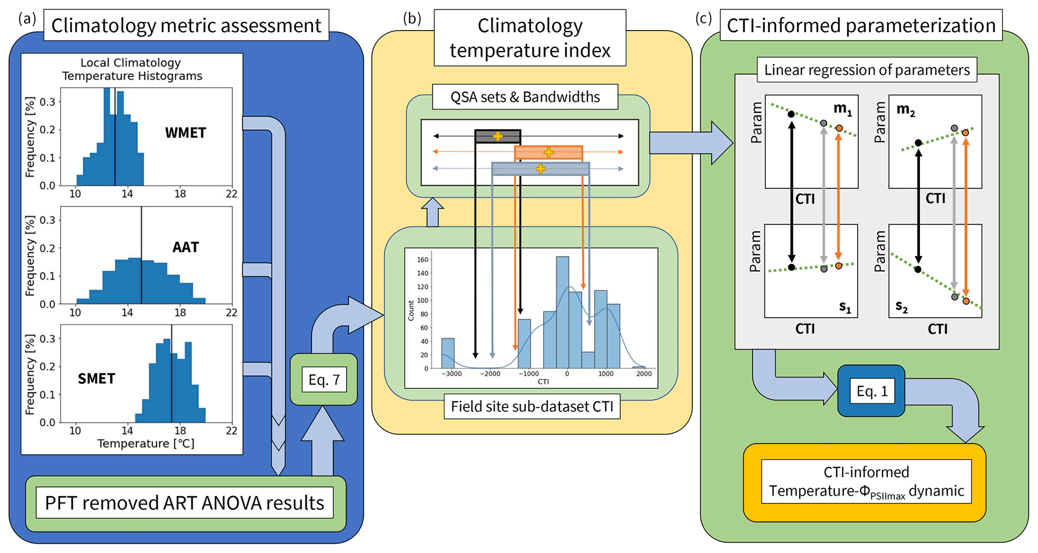
Figure 2 A pipeline of incorporating climatological temperature's effect on the modeled parameterization of temperature tolerance and resilience of vegetative Φ_PSIImax, including (a) quantifying the histogram frequency distribution of three climatological temperature metrics (WMET, SMET, AAT) within the field site sub-dataset and their contributions to the prediction deficiency estimated by the developed PFT-specific temperature–Φ_PSIImax functions using ART ANOVA. WMET and SMET refer to the median experienced temperature in the winter and summer, respectively, while AAT refers to the annual average temperature calculated using the 0.5° × 0.5° CRUNCEP v.7 hourly temperature dataset over 1985–2016. (b) Calculating the climatology temperature index (CTI) for all data in the field site sub-dataset using results of ART ANOVA and Eq. (7), with the resulting distribution of CTI values shown in a histogram, and the quantile system approach (QSA)-based data grouping and parameter ($m_{\mathrm{1}},m_{\mathrm{2}},s_{\mathrm{1}},s_{\mathrm{2}}$) estimation. Here, QSA refers to using multiple bandwidths (shown as different color boxes) to group data for fitting Eq. (1), varying the range of the selected data across the whole dataset, and recording the central CTI (shown as the gold cross) and resulting parameters. (c) The CTI-informed parameterization of temperature–Φ_PSIImax dynamic, which linearly regressed each of the four parameters ($m_{\mathrm{1}},m_{\mathrm{2}},s_{\mathrm{1}},s_{\mathrm{2}}$) on the corresponding central CTI values resulting in a CTI-informed parameter estimation for the temperature–Φ_PSIImax function.

2.3.1 Assessment of climatology temperature metrics

There were 25 locations ranging from [35.4° S, 107° W to 69.25° N, 140° E] within the field site sub-dataset (Fig. 1d). For each location, we used hourly temperature from the 0.5° × 0.5° CRUNCEP v.7 forcing dataset (Viovy, 2018) between 1985 and 2016 to quantify three climatology temperature metrics: the average annual temperature (AAT), the summer median experienced temperature (SMET), and the winter median experienced temperature (WMET). To isolate a summer (winter) season based on temperature, a rolling 3-month average was performed to find the warmest (coldest) consecutive 3 months. From these 3 months, the median temperature served as the location's summer (winter) median experienced temperature over 30 years (Fig. 2a). In addition, an AAT for each location was estimated by first calculating the annual mean temperature of each year and then averaging over all 30 years (Fig. 2a).

2.3.2 Quantifying climatology impact on prediction efficiency

To examine how climatology metrics affect the prediction efficiency of the developed PFT-specific model, an aligned rank transform analysis of variance (ART ANOVA) was performed. We calculated the residues (X) between collected Φ_PSIImax values (Φ_PSIImax,O) and predicted Φ_PSIImax values (Φ_PSIImax,P) given by a specific temperature–Φ_PSIImax function parameterization (Eq. 5).

$$\begin{array}{}\text{(5)}& X={\mathrm{\Phi }}_{\text{PSIImax,P}}-{\mathrm{\Phi }}_{\text{PSIImax,O}}\end{array}$$

We then analyzed X with ART ANOVA. ART ANOVA is a nonparametric test of data variation with multiple factors. It allows a determination of the contribution of variance by each factor and the interaction effect of multi-factors when assumptions of equal sample sizes within each factor level needed for conventional ANOVA parametric tests are not met (Leys and Schumann, 2010). Here the divisions of each climatology temperature metric level were determined via the Freedman–Diaconis rule (Freedman and Diaconis, 1981) as follows.

$$\begin{array}{}\text{(6)}& \text{Bin\hspace{0.17em}\hspace{0.17em}width }=\mathrm{2}\mathrm{IQR}\times n^{-\mathrm{1}/\mathrm{3}}\end{array}$$

Here n is the number of residues used in the test and IQR is their interquartile range.

Following Wobbrock et al.'s (2011) ART ANOVA analysis procedure, we first performed a preprocessing step to align the X of each Φ_PSIImax value in the field site sub-dataset for each main effect of the predictors (SMET, WMET, AAT), as well as their two-way and three-way effects, using Eqs. (B1)–(B7) (see Appendix B). Second, the aligned X values for each effect were then ranked from smallest to largest, with ties between M numbers of X values resulting in the sum of the ranks divided by M. Finally, a standard ANOVA test was performed on the ranks of the aligned X values for each effect and their combinations. Here all main predictor effects and their two-way and three-way interaction effects were induced at each instance of ANOVA analysis, while only the total sum of the squares of errors of the tested effect was kept. Also, the total sum of squares of the residuals from each ANOVA analysis was recorded and averaged to represent the final sum residual that failed to be explained by the three climatology temperature metrics and their interaction effects. The resulting total sum of the squares is each effect's sum of squares and the residual term. The ratio of each effect's sum of squares to the total sum of squares is a measure of the explained prediction error resulting from a specific temperature–Φ_PSIImax model by SMET, WMET, AAT, and their interactions.

Besides performing the above ART ANOVA analysis to explain the contribution of climatological temperature to the prediction error of the 12 PFT-specific temperature–Φ_PSIImax functions developed, we also performed the second ART ANOVA analysis to examine the contribution of three temperature metrics and their interactions to the prediction residues by the general temperature–Φ_PSIImax function derived using all data in the field site dataset. The results of two ART ANOVA were then compared (see Appendix D).

2.3.3 Climatology temperature index

To create a single predictor index that incorporates the effect of three temperature metrics on predicting the temperature response function of Φ_PSIImax, the climatology temperature index (CTI) was created (Fig. 2b). This index, which was associated with each Φ_PSIImax measurement in the field site sub-dataset, was determined by creating a linear combination of SMET, WMET, and AAT (Eq. 7) based on the results from the above ART ANOVA analysis. For each Φ_PSIImax measurement p in the field site sub-dataset, its CTI value is given as

$$\begin{array}{}\text{(7)}& \begin{array}{rl}{\text{CTI}}_p=& a_{\mathrm{1}}{\text{SMET}}_p^{\ast }+a_{\mathrm{2}}{\text{WMET}}_p^{\ast }+a_{\mathrm{3}}{\text{AAT}}_p^{\ast }\\ & +a_{\mathrm{4}}\left({\text{SMET}}_p^{\ast }\times {\text{WMET}}_p^{\ast }\right)\\ & +a_{\mathrm{5}}\left({\text{SMET}}_p^{\ast }\times {\text{AAT}}_p^{\ast }\right)\\ & +a_{\mathrm{6}}\left({\text{WMET}}_p^{\ast }\times {\text{AAT}}_p^{\ast }\right)\\ & +a_{\mathrm{7}}\left({\text{SMET}}_p^{\ast }\times {\text{WMET}}_p^{\ast }\times {\text{AAT}}_p^{\ast }\right).\end{array}\end{array}$$

Here a_L ($L=\mathrm{1},\mathrm{2},\mathrm{\dots }\mathrm{7}$) is the relative contribution of each climatological temperature metric and their interactions to variations in prediction residues by each temperature–Φ_PSIImax function (PFT-specific or general) as shown in Fig. 5. The * denotes the deviation from the mean of all the respective climatology index values within the field site dataset.

2.3.4 Quantile system approach for parameterizing climatology's effect on temperature resilience and tolerance of Φ_PSIImax

To incorporate the climatology factors into the parameterization of the temperature–Φ_PSIImax function (Eq. 1), we quantified the dependence of the parameters (m₁, m₂, s₁, s₂) on CTI using the field site sub-dataset. Ideally, the field site sub-dataset would cover diverse climatological temperature conditions, be distributed consistently across the full global range of CTI values, and contain statistically sufficient data for all PFTs, but this is not the case. The 709 available measurements represent a limited, non-uniform range of climatology temperature metrics (histogram distribution of data in Fig. 2b). We overcome this data limitation by generating one CTI dependence function for each parameter in Eq. (1) using all data from the field site sub-dataset and the quantile system approach (QSA), which was developed to navigate the small sample size and inconsistent CTI value distribution by performing the following three steps.

First, to identify ranges of CTI upon aggregation can overcome the non-uniform distribution of CTI values, we ranked from least to greatest all field site sub-dataset Φ_PSIImax values and their corresponding experimentally measured temperature values based on the CTI values at the location of the associated studies. A bandwidth (B) is defined as a quantile range of CTI values in the field site sub-dataset and recorded as a percentile. The corresponding Φ_PSIImax and experimentally measured temperature within the bandwidth B were selected and composed into a CTI-labeled sub-dataset. The central value of the range of CTI selected in this manner, here being the average of the upper and lower bounds within B, was used as a description of CTI for the corresponding CTI-labeled sub-dataset. We then used the sub-dataset and its central CTI value to define a “QSA set”, which was then connected to the parameters of Eq. (1) through fitting. This bridges the parameters (m₁, m₂, s₁, s₂) to the QSA set's associated climatology. The maximum value of Φ_PSIImax parameter (a) in Eq. (1) was assumed to be independent of CTI and kept the same as the fitted value based on the PFT-specific parameterizations in Sect. 2.2. Four bandwidths (B = 66 %, 50 %, 33 %, 25 %) were chosen: the maximum bandwidth (B = 66 %) was chosen due to larger selections generating QSA sets too similar in composition to regress fitted parameters on the central CTI values of the QSA sets. The minimum bandwidth (B = 25 %) was chosen as a cutoff due to smaller B values containing too many QSA sets of fewer than 30 measurements selected to fit Eq. (1), which caused rapidly fluctuating parameterizations to occur.

Second, to analyze how varying central CTI values, which serve to inform climatology, influenced the fitted parameters in Eq. (1), QSA sets were generated for each bandwidth starting from the bounds [0, B%] till [100 %–B, 100 %], with a step size of 1 %. Each set was fit to Eq. (1), generating (100–B) QSA sets per bandwidth B. All QSA sets across all chosen B values had their resulting parameters (m₁, m₂, s₁, s₂), associated with their central CTI values, aggregated, totaling 224 sets of CTI-related parameterization results.

Finally, to mitigate the existence of noisy data impact on the regression of fitted parameters on the central CTI values of QSA sets, we applied a univariate smoothing algorithm (Appendix C) similar to that outlined in Cleveland et al. (1988) to smooth the fitted parameters and corresponding central CTI values of the QSA sets before performing the final regression analysis. This new composite set of smoothed QSA set parameters was then regressed on the associated QSA set central CTI values (Fig. 2c) to quantify the impact of climatological temperature on the model parameters. This provided four CTI-dependent equations of the parameters (m₁, m₂, s₁, s₂) in Eq. (1), informing the climatological impacts on temperature tolerance and resilience of vegetative Φ_PSIImax.

2.3.5 Comparison of CTI-informed and PFT-specific parameterizations of the temperature–Φ_PSIImax relationship

To assess the improvement in this CTI-informed parameterization for the temperature–Φ_PSIImax dynamic prediction, the cumulative sum of the prediction residuals from this CTI-informed parameterization was examined along the ascending order of CTI values and compared to the counterparts from the PFT-specific parameterizations. The range of CTI over which the sum of residuals is reduced implies improved predictive power.

To further identify the geographical regions within which the climatology's effect on the temperature–Φ_PSIImax relationship of a specific PFT was important to consider, we quantified the differences in estimated temperature resilience (s₁, s₂) and tolerance metrics (T_MC, T_MH) between CTI-informed and PFT-specific parameterizations at each 0.5° × 0.5° grid cell across space. This comparison was constrained in the regions where CTI-informed parameterization showed improvement in prediction over the PFT-specific counterpart or could be compared to each other. Within this constrained domain, the CTI value at each grid cell was calculated using the 1985–2016 CRUNCEP v.7 hourly temperature dataset (Viovy, 2018) following the method introduced in Sect. 2.3.2. This was then applied to estimate CTI-based temperature resilience (s₁, s₂) and tolerance metrics (T_MC, T_MH) for the corresponding grid cell using the generated CTI-dependent m₁, m₂, s₁, and s₂ parameter equations (Sect. 2.3.4). Covered PFTs at each grid cell were identified using the MODIS-derived present-day land cover data (Lawrence and Chase, 2007; Lawrence et al., 2016). To focus the study on PFTs that consistently reside within the CTI-constrained domain, only PFTs whose total cover areas within the domain were at least 50 % of their global coverage were considered. PFT-specific temperature resilience (s₁, s₂) and tolerance metrics (T_MC, T_MH) at each PFT-covered grid cell were estimated using PFT-specific parameterization (Sect. 2.2). The CTI-based parameters at each grid cell were finally compared to the corresponding parameters from PFT-specific functions to identify the region at which climatological temperatures' impact on the temperature tolerance and resilience of a specific PFTs' Φ_PSIImax values needs to be considered.

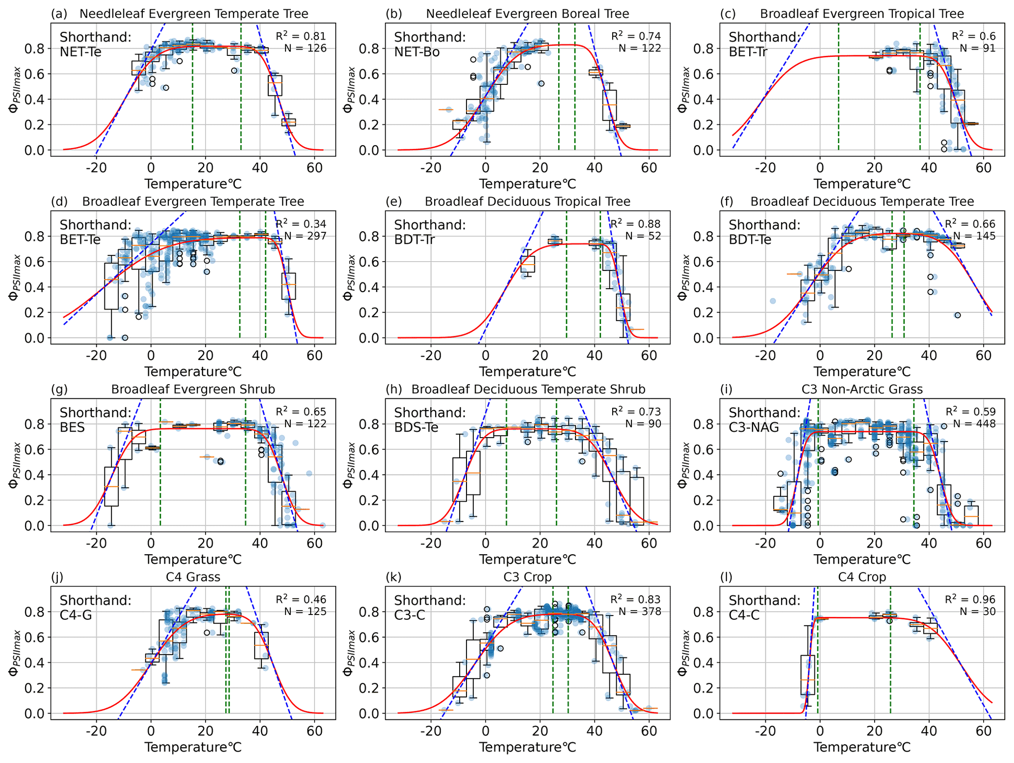
Figure 3 PFT-specific parameterization results for 12 plant functional types, with the abbreviations (a) NET-Te, (b) NET-Bo, (c) BET-Tr, (d) BET-Te, (e) BDT-Tr, (f) BDT-Te, (g) BES, (h) BDS-Te, (i) C3-NAG, (j) C4-G, (k) C3-C, and (l) C4-C. The red line is the resulting PFT-specific model (Eq. 1). The dotted blue lines depict the slope of the model at the temperature m₁ (m₂) where Φ_PSIImax declines 50 % from maximum a, and its slope is the resiliency parameter s₁ (s₂) for cold (hot) temperatures. The left (right) vertical dotted green lines depict the tolerance parameter T_MC (T_MH) for cold (hot) temperatures, and the region between them is the range of temperatures at which Φ_PSIImax remains constant.

3 Results

3.1 Temperature response of Φ_PSIImax varies depending on PFT

Our results showed that the rectangular function (Eq. 1) was able to capture the temperature dependence of Φ_PSIImax across all the gathered PAM fluorometry data. The cross-validation test resulted in a statistically consistent R² of 0.49 ± 0.03 in both iterations (p value = 0.87). Data availability allowed for quality modeling of the PFT-specific temperature–Φ_PSIImax functions for 12 plant functional types. Temperature variability explained more than 60 % of Φ_PSIImax variations (R² > 0.60) for most of the PFTs (Fig. 3), except for broadleaf evergreen temperate trees (BET-Te), C3 non-Arctic grasses (C3-NAG), and C4 grasses (C4-G) with R² values of 34 %, 59 %, and 46 %, respectively (Fig. 3d, i, j). All PFTs followed the expected features of maintaining maximum Φ_PSIImax values of around 0.8 over a general temperature range from 16–34 °C. Additionally, Φ_PSIImax significantly declined when temperatures get too hot (cold), depending on diverse temperature tolerances and resiliency of different PFTs.

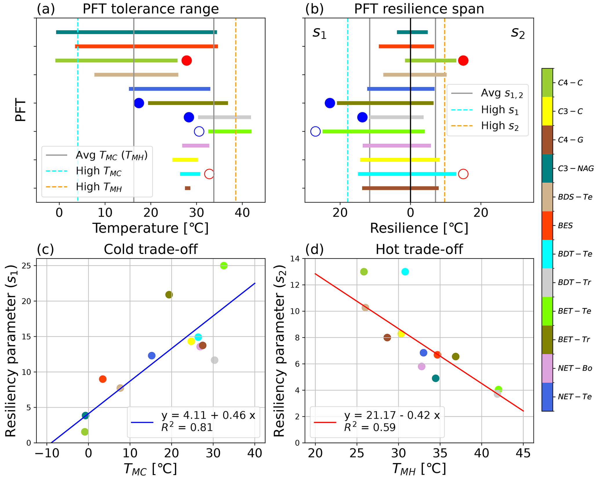
Figure 4 Visualization of the PFT-specific tolerance and resilience parameters, including (a) the tolerance range of temperatures across which Φ_PSIImax remains consistently near the maximum modeled value (a) for the 12 modeled PFTs, as defined by the T_MC and T_MH values; (b) the cold (s₁) and hot (s₂) temperature resiliencies of the 12 modeled PFTs, labeled in the upper left and right corners, respectively; (c) the trade-off between cold tolerance (T_MC) and resilience (s₁); and (d) the trade-off between hot tolerance (T_MH) and resilience (s₂) for the 12 modeled PFTs. PFTs with a filled blue circle next to their parameter value in panels (a, b) were not used in determining the respective cold temperature parameters' mean and standard deviation, and similarly PFTs with filled red circles next to their parameter values in panels (a, b) were not used in determining the respective hot temperature parameters' mean and standard deviation. Open circles of red or blue in panels (a, b) identify a PFT with data such that the resulting cold or hot parameter results should be taken with some caution. The gray lines in panels (a, b) are the average parameter values. The high cold and high hot tolerance classifications are based on the PFT having a T_MC or T_MH value that is 1σ less than or greater than the respective average tolerance value and are represented by the dashed blue and orange lines, respectively. The high-resiliency parameters are defined both as having s₁ or s₂ that is 1σ greater than the respective average value across considered PFT values.

3.1.1 Tolerance

The T_MC and T_MH tolerance metrics of 12 PFTs varied from −0.7 to 32.6 °C and from 25.8 to 42 °C, respectively, indicating large differences in cold and hot temperature tolerance of Φ_PSIImax values among 12 PFTs (Fig. 4a). Due to data gaps (Fig. 3c, e, and l), the T_MC of broadleaf evergreen tropical trees (BET-Tr) and broadleaf deciduous tropical trees (BDT-Tr) and the T_MH of C4 crops (C4-C) were not used in mean and standard deviation (SD) calculations of T_MC and T_MH. The mean and SD values of T_MC and T_MH for the rest of the PFTs are 16.3 ± 12.2 and 33.8 ± 4.8 °C, respectively. Among the 12 PFTs, the cold and hot tolerance responses of needleleaf evergreen temperate trees (NET-Te) are closest to the average, with values of 15.2 and 33 °C for T_MC and T_MH, respectively (Fig. 4a). The Φ_PSIImax of C3 non-Arctic grasses (C3-NAG) showed the widest range of temperature tolerance to both cold and hot temperatures, ranging from −0.7 to 34.5 °C (Fig. 4a). Broadleaf evergreen shrubs (BESs) showed a similar range of tolerance temperatures: 3.5 to 34.7 °C (Fig. 4a). In contrast, needleleaf evergreen boreal trees (NET-Bo), broadleaf deciduous temperate trees (BDT-Te), C4 grasses (C4-G), and C3 crops (C3-C) showed weaker Φ_PSIImax tolerance to both hot and cold temperature compared to the average, ranging from 26.9–32.8, 26.4–30.8, 27.5–28.6, and 26.1–32.1 °C ^∘, respectively (Fig. 4a).

Most PFTs do not have simultaneously strong and weak tolerances to high and low temperature extremes; i.e., high T_MH values rarely occurred with low T_MC values (strong temperature extreme tolerance), and low T_MH values rarely occurred with high T_MC values (weak temperature extreme tolerance). Broadleaf evergreen tropical trees (BET-Tr), broadleaf evergreen temperate trees (BET-Te), and broadleaf deciduous tropical trees (BDT-Tr) all had above-average hot tolerance, with T_MH values of 36.9, 42, and 41.9 °C, respectively (Fig. 4a). BDT-Tr and BET-Te were PFTs with strong hot tolerance, defined as T_MH 1 standard deviation higher than the mean (Fig. 4a). The T_MC value of BET-Te indicated a decline at temperatures below 32.6 °C, although there was high variability in its Φ_PSIImax values at each temperature below 32.6 °C. The declining trend of the T_MC values of BET-Te gradually became obvious when temperatures fell below −7.7 °C (Fig. 3d). BET-Tr (Fig. 3c) and BDT-Tr (Fig. 3e) lacked cold temperature measurements. Broadleaf deciduous temperate shrubs (BDS-Te) had a strong cold tolerance, with a T_MC of 7.7 °C, but did not have hot temperature tolerance (T_MH = 26 °C), unlike the other PFTs of C3-NAG and BES with strong cold tolerance (Fig. 4a). C4 crops (C4-C) were strongly cold tolerant (T_MC = −0.86 °C), but due to low data availability, the hot temperature responses of this group were unclear (Fig. 3l).

3.1.2 Resilience

The s₁ and s₂ resilience parameters of 12 PFTs varied from 1.56 to 24.9 °C and from 3.7 to 12.9 °C, respectively, indicating that the resilience of Φ_PSIImax values to cold and hot temperature varied with PFT (Fig. 4b). A strong cold or hot resilience was signalled by a large s₁ or s₂ value and a slower decline in Φ_PSIImax as temperature changes beyond the ideal tolerance range. Due to data gaps (Fig. 3c, e, and l), the s₁ of broadleaf evergreen tropical trees (BET-Tr) and broadleaf deciduous tropical trees (BDT-Tr) and the s₂ of C4 crops were not used in mean and SD calculations of s₁ and s₂. The mean and SD values of s₁ and s₂ for the rest of PFTs were 11.6 ± 6.2 and 7.1 ± 2.6 °C, respectively. Among 12 PFTs, NET-Te had the closest-to-average resilience to both low and high temperature (s₁ = 12.3 °C; s₂ = 6.8 °C) (Fig. 4b). The Φ_PSIImax values of the C3-NAG had the least cold and second least hot temperature resilience, with an s₁ and s₂ of 3.9 and 4.9 °C, respectively (Fig. 4b). The next least-resilient PFT overall was BES, with an s₁ and s₂ of 8.99 and 6.7 °C, respectively (Fig. 4b). There was no PFT that had both strong cold and strong hot temperature resilience, as defined by one SD more than the mean. The most temperature-resilient PFT overall was BDT-Te, with an s₁ and s₂ of 14.9 and 12.99 °C, respectively (Fig. 4b). Other PFTs that had higher than average cold and hot resilience include C4-G (s₁ = 13.7 °C; s₂ = 7.99 °C) and C3-C (s₁ = 14.3 °C; s₂ = 8.3 °C) (Fig. 4b).

PFTs that had strong cold resilience but weak hot resilience included NET-Bo (s₁ = 13.6 °C; s₂ = 5.8 °C), BET-Tr (s₁ = 20.9 °C; s₂ = 6.6 °C), BET-Te (s₁ = 24.9 °C; s₂ = 4.0 °C), and BDT-Tr (s₁ = 11.7 °C; s₂ = 3.7 °C) (Fig. 4b). BET-Te was a PFT with strong cold resilience. More cold temperature measurements for BET-Tr and BDT-Tr were needed to validate the current fitting result (Fig. 3c and e). PFTs that had strong hot resilience but weak cold resilience included BDS-Te (s₁ = 7.7 °C; s₂ = 10.3 °C) and C4-C (s₁ = 1.56 °C; s₂ = 12.9 °C) (Fig. 3h and l). BDT-Te, BDS-Te, and C4-C were all PFTs with strong hot resilience, although more hot temperature observations for BDT-Te and C4-C are still needed for validating this fitting result.

3.1.3 Tolerance–resilience trade-off in PFT

There was a positive correlation between s₁ parameters and T_MC parameters but a negative correlation between s₂ parameters and T_MH parameters for 12 PFTs (Fig. 4c and d). These results indicated a clear trend in temperature responses of the various PFTs' Φ_PSIImax values, in which the more temperature-resilient PFTs were less temperature tolerant, and vice versa. The s₁ and T_MC parameters of BET-Te (24.9 °C, 32.6 °C) indicated BET-Te was the most resilient but one of the least tolerant to cold temperature, whereas C4-C with a low s₁ (1.56 °C) and the coldest T_MC (−0.9 °C) was extremely tolerant but one of the least resilient to cold temperature (Fig. 4c). Besides C4-C and BDT-Te, which needed more observations at high temperature for validating their fitted high resilience to hot temperature, BDS-Te was the third most resilient (10.3 °C) but the least tolerant (26 °C) to hot temperatures (Fig. 4d). In contrast, C3-NAG showed both strong tolerance to cold temperature (T_MC = −0.9 °C) and high temperature (T_MH = 38.9 °C) but was the second least cold (s₁ = 3.85 °C) and third least hot resilient (s₂ = 4.9 °C) to temperature (Fig. 4c and d).

Based on this trade-off between temperature tolerance and resilience of the PFTs' Φ_PSIImax temperature response, we can classify 12 PFTs into three groups with different life history strategies of light partitioning in response to extreme temperatures. PFTs within the cold and hot temperature tolerance group (strongly temperature tolerant), including BES and C3-NAG, held the maximum Φ_PSIImax value (∼ 0.8) within a wide (> 20 °C) temperature range. In contrast, PFTs within the cold and hot temperature resilience group (strongly temperature resilient), including BDT-Te, NET-Bo, C4-G, and C3-C, can still keep higher Φ_PSIImax values in response to a large increase in hot temperature or decrease in cold temperature. NET-Te is a PFT with medium temperature tolerance and resilience in between these two extreme groups. BET-Te, BDT-Tr, BET-Tr, C4-C, and BDS-Te are the temperature specialist group. They have a strong tolerance to either hot or cold temperatures (but not both) and are strongly resilient in opposite temperature extremes. Among them, C4-C and BDS-Te were PFTs with strong cold tolerance and strong hot resilience, whereas BET-Tr and BET-Te were PFTs with strong cold resilience and strong hot tolerance. BDT-Tr was only tolerant to hot temperatures.

3.2 Climatology's influence on the temperature–Φ_PSIImax relationship

To test the hypothesis that climatological temperature shifts different PFT's temperature–Φ_PSIImax responses toward converged responses to the climatology of their “similar” local habitat, we generated a general climatology-informed temperature–Φ_PSIImax function by estimating the global distribution of the climatology temperature index (CTI) and quantifying its regulations on tolerance and resilience parameters in Eq. (1) across the globe (Sect. 3.2.1). To identify the specific region within which the impact of climatological temperatures on the temperature tolerance and resilience of Φ_PSIImax values needs to be considered, we quantified the spatial distributions of the CTI-informed parameters (m₁, m₂, s₁, s₂) and tolerance metrics (T_MC, T_MH) (Sect. 3.2.2) and compared them with their PFT-specific counterparts (Sect. 3.2.3).

3.2.1 CTI global pattern and its regulation on the temperature tolerance and resilience of Φ_PSIImax values

The ART ANOVA analyses indicated that annual average temperature (AAT), the median experienced temperature in the winter (WMET) and summer (SMET), and their interactions could explain around 96 % of the variances in prediction residues generated with PFT-specific temperature–Φ_PSIImax functions (see Appendix D). Therefore, we estimated the CTI as the linear combination of AAT, WMET, and SMET, as well as their interactions (Eq. 7), using their relative contribution to variations in prediction residues by PFT-specific temperature–Φ_PSIImax functions calculated from the ART ANOVA analysis. We employed this method to quantify the CTI distribution at each 0.5° × 0.5° grid cell across the globe using the 1985–2016 CRUNCEP v.7 hourly temperature dataset (Viovy, 2018).

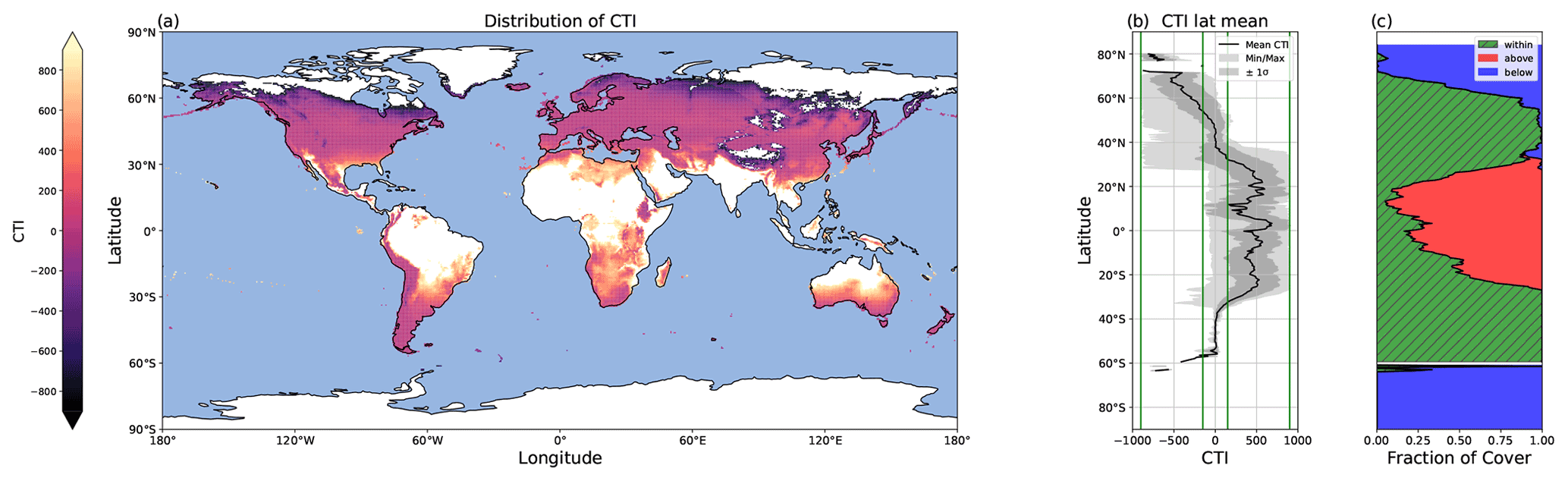
Figure 5 Global distribution of CTI values and their latitudinal trends. (a) Map depicting the global distribution of CTI for grid cells at which |CTI| ≤ 900. (b) Latitude mean CTI values of all land grid cells with |CTI| no larger than |900| (black line), with both the minimum and maximum (light gray), as well as ± the standard deviation (σ) (dark gray). Four green lines from the left to the right demonstrate the CTI bounds of −900, −150, 150, and 900. The range of 150 ≤ |CTI| ≤ 900 refers to the CTI range at which the temperature–Φ_PSIImax relationship was improved by CTI-informed parameterization compared to the PFT-specific parameterization. (c) The percentages of land grid cells at each latitude that were below (blue), within (hatched green), and above (red) the range of |CTI| ≤ 900.

The global distribution of CTI showed a clear latitude gradient. A large area of the mid-latitudes had CTI values close to zero (Fig. 5a and b), indicating these regions had very similar CTI indices to the mean state, which referred to the mean of all the respective CTI values within the field site sub-dataset. The CTI values trended to be more positive from the mid-latitude to the tropical regions and more negative from the mid-latitude to the polar regions (Fig. 5a and b).

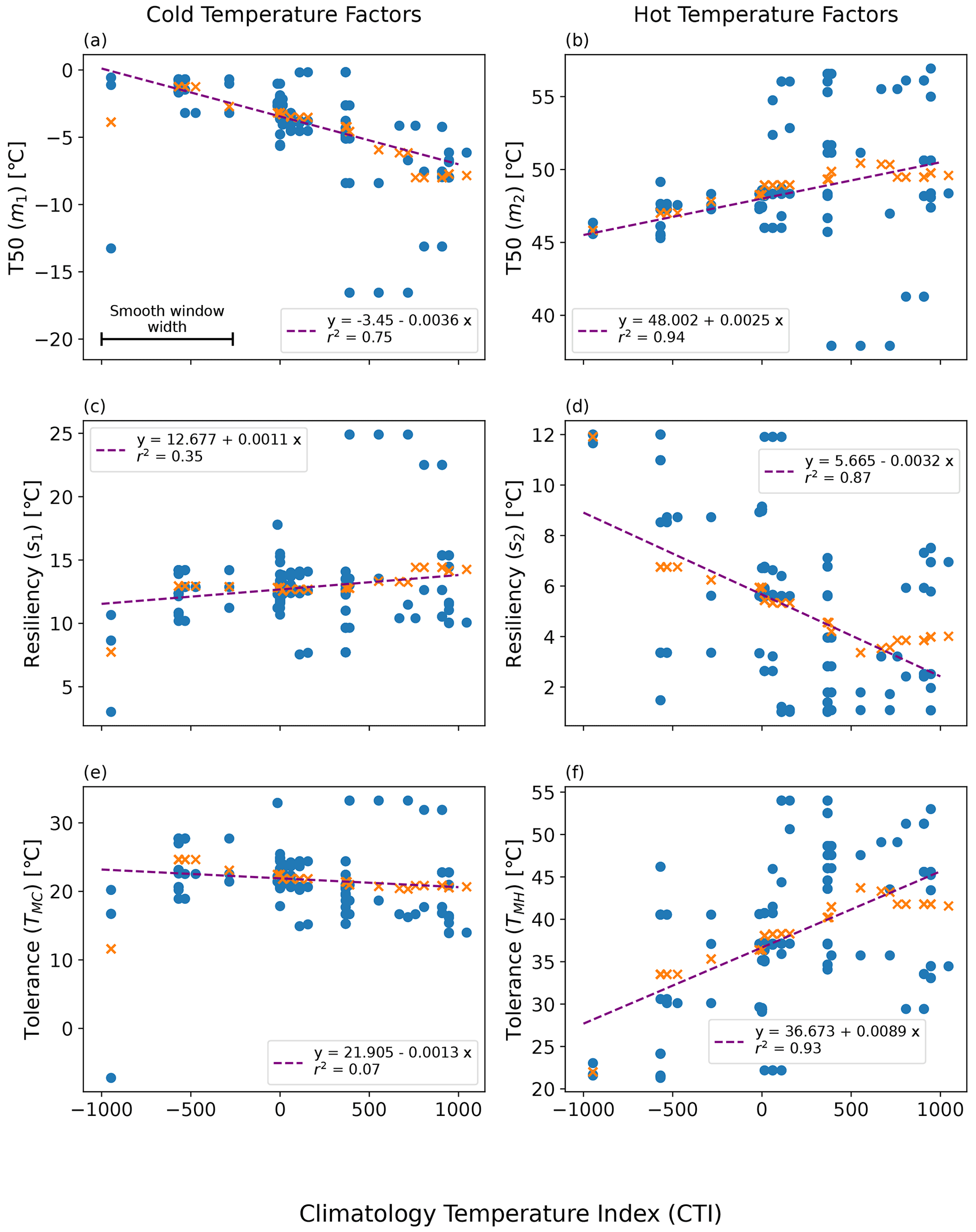
Figure 6 Linearly smoothed MID regression of temperature resilience and tolerance parameters on the climatological temperature index (CTI) using the QSA approach: (a) m₁-CTI, (b) s₁-CTI, (c) m₂-CTI, (d) s₂-CTI, (e) T_MC-CTI, and (f) T_MH-CTI. Here m₁, m₂, s₁, and s₂ refer to the original four parameters in Eq. (1). The original estimation of each parameter and the corresponding mean CTI of a QSA set are displayed in blue-filled circles. The smooth window width featured in (a) the top left plot is centered upon each QSA result, and all values within that CTI range are averaged. The orange cross symbols (x) are the resulting smoothed values, which were then run through a linear least-square regression. The resulting regressions are displayed as purple lines.

The resulting regression of each parameter on CTI showed a strong correlation between CTI and each model parameter (m₁, m₂, s₁, s₂) in Eq. (1), in addition to the tolerance values (T_MC, T_MH). The strongest CTI dependence was with the hot temperature parameters (m₂, R² = 0.94; s₂, R² = 0.87) (Fig. 6b and d). Cold temperature parameters had slightly less dependence on CTI (m₁, R² = 0.75; s₁, R² = 0.35) (Fig. 6a and c). The CTI values were negatively correlated to the cold T₅₀ parameter m₁ (Fig. 6a) but positively correlated to the cold resilience parameter s₁ (Fig. 6c). In contrast, the CTI values were positively correlated to the hot T₅₀ parameter m₂ (Fig. 6b) but negatively correlated to the hot resilience parameter s₂ (Fig. 6d). Built upon the regressions of m₁, m₂, s₁, and s₂ on CTI, the regression of T_MC and T_MH on CTI showed that T_MC is negatively but not significantly correlated to CTI (R² = 0.07), whereas T_MH was positively and significantly correlated (R² = 0.93) to CTI (Fig. 6e and f). These results indicated that the climate condition in the habitat in part affected the temperature tolerance and resilience of Φ_PSIImax. Taking the averaged CTI of the field site sub-dataset as a reference, the Φ_PSIImax values of plants in the warmer than average habitats (higher positive CTI) had a stronger tolerance to hot temperatures (Fig. 6f) at the cost of lower hot temperature resilience (Fig. 6d). Similarly, the Φ_PSIImax values of plants located in colder than average habitats (lower negative CTI) had a lower cold temperature resilience (Fig. 6c) but no statistically significant change in cold temperature tolerance with CTI (Fig. 6e).

The regression of each model parameter (m₁, m₂, s₁, s₂) in Eq. (1) on CTI, denoted as the CTI-informed parameterizations of the temperature–Φ_PSIImax relationship, facilitated the prediction of the temperature responses of plant Φ_PSIImax in certain CTI ranges. Compared to the prediction by PFT-specific parameterization, the CTI-informed parameterization improved the accuracy of Φ_PSIImax prediction by 4.3 % on average in the land grid cell with 150 ≤ |CTI| ≤ 900 and held comparable in the region with |CTI|  < 150 (Fig. D2). This land area with |CTI| ≤ 900 accounted for ∼ 53 % of the earth's land area, which was distributed in the latitudinal bands of 60° S–80° N, especially in the latitudinal bands of 30–60° S and 30–70° N. At this latitude range, almost 100 % of land grid cells had |CTI| ≤ 900 (Fig. 5c). Spatially, these regions included much of South America outside of the Amazon, Africa, and most of Canada and Russia (Fig. 5a). The upper Andes and Mexico's Sierra Madre ranges, a large region in Ethiopia, and much of Libya had CTI that is much lower than the surrounding regions at the same latitude, falling with the CTI bounds of improved or comparable predictive power. Notable regions that fell outside the bounds were both the Amazon and Indonesian rainforests, as well as the Indian subcontinent and much of the Congo rainforest (Fig. 5a). Our results highlighted that climatology's effect on temperature tolerance and resilience of Φ_PSIImax values needs to be considered in these regions with |CTI| ≤ 900.

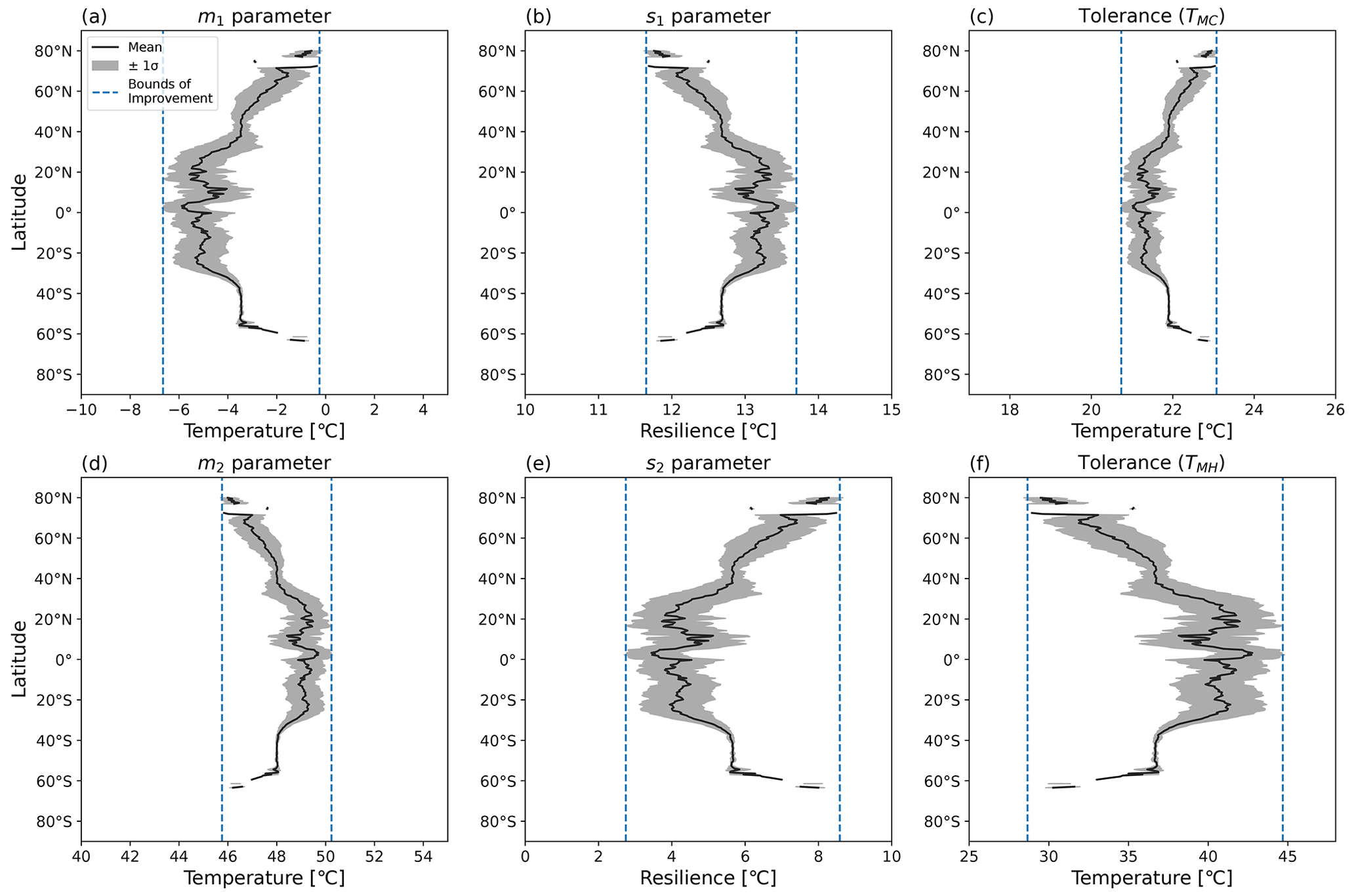
Figure 7 Latitudinal mean and standard deviation (σ) of CTI-informed model parameters, including (a, b) cold and hot T₅₀ parameters (m₁,m₂) at which Φ_PSIImax values decrease by 50 %, (c, d) cold and hot temperature resilience parameters (s₁,s₂) in Eq. (1), and (e, f) derived cold and hot temperature tolerance metrics (T_MC, T_MH) for land grid cells with |CTI| < 900.

3.2.2 Latitudinal variation in CTI-informed temperature tolerance and resilience of plant Φ_PSIImax

Using the CTI-informed parameterizations, the cold and warm T₅₀ parameters (m₁, m₂), temperature resilience parameters (s₁, s₂), and resultant temperature tolerance parameters (T_MC, T_MH) of vegetative Φ_PSIImax values within the region of |CTI| ≤ 900 were estimated and showed clear latitudinal gradients across the globe. The latitudinal mean m₁ increased from −5.5 to −3.5 °C across the transient band moving from tropical latitudes to mid-latitudes (30–40° N and S) and from −3.5 to almost 0 °C from mid-latitudes to high latitudes (50–80° N and 55–65° S) but held values around −5.5 °C in the tropics (30° N–30° S) and around −3.5 °C in the mid-latitudes (40–50° N and 40–60° S) (Fig. 7a). Parameter s₁ also showed less latitudinal variability around 30° N–30° S and the mid-latitude band around 40–50° N and 40–60° S but an inverse trend compared to the latitudinal variability in m₁, decreasing from 13.2 °C in tropical latitudes (30° N–30° S) to 12.7 °C in mid-latitudes (30–40° N and S) and from 12.7 °C in mid-latitudes to 11.6 °C in high latitudes (50–80° N and 55–65° S) (Fig. 7b). The cold tolerance T_MC, being a linear combination of m₁ and s₁, exhibited a similar trend as m₁, with almost 2 °C of variation across latitudes, which is smaller in comparison to the latitudinal variability in m₁ (Fig. 7c). These results indicated the Φ_PSIImax in temperate habitats across 40–50° N and 40–60° S had similar cold temperature T₅₀ and cold temperature resilience and tolerance. However, Φ_PSIImax tended to have a higher cold temperature T₅₀ and be less tolerant and resilient to cold temperatures from 30–40° N and S, from 50–80° N, and from 55–65° S.

The latitudinal mean m₂ decreased from 49.2 to 47.9 °C from 20–40° N and S and from 47.9 to 45.8 °C from middle to high latitude (50–80° N, 55–65° S), with a maximum value of 49.7 °C across the tropics and an almost constant value of 47.9 °C across 40–50° N and S (Fig. 7d). Similar to the relationship between the latitudinal trend of m₁ and s₁, the latitudinal mean s₂ increased across latitudes where the m₂ decreased, with a greater latitudinal variation compared to s₁ (Fig. 7e). Similar to m₁ and s₁, m₂ and s₂ also had less variation in the tropic (30° N–30° S) and the mid-latitude band around 40–50° N and 40–60° S. The hot tolerance T_MH, being a linear combination of m₂ and s₂, exhibited a similar trend to m₂, with around 15 °C of variation across latitudes being larger in comparison to the latitudinal variability in m₂ (Fig. 7f). These findings also suggested that the vegetation at temperate habitats across 40–50° N and S had a similar response of the Φ_PSIImax value to hot temperature. In contrast, the Φ_PSIImax values tended to be less tolerant but more resilient to hot temperature across the tropical-to-middle-latitude transition regions (30–40° N and S) and middle-to-high-latitude transition regions (50–80° N, 55–65° S).

Corresponding to the latitudinal pattern of T₅₀, resilience, and tolerance parameters (Fig. 7) with the spatial pattern of CTI values (Fig. 5), Φ_PSIImax values became less cold tolerant and resilient and less hot tolerant but more hot resilient along warm-to-cold climatological gradients (CTI gradients).

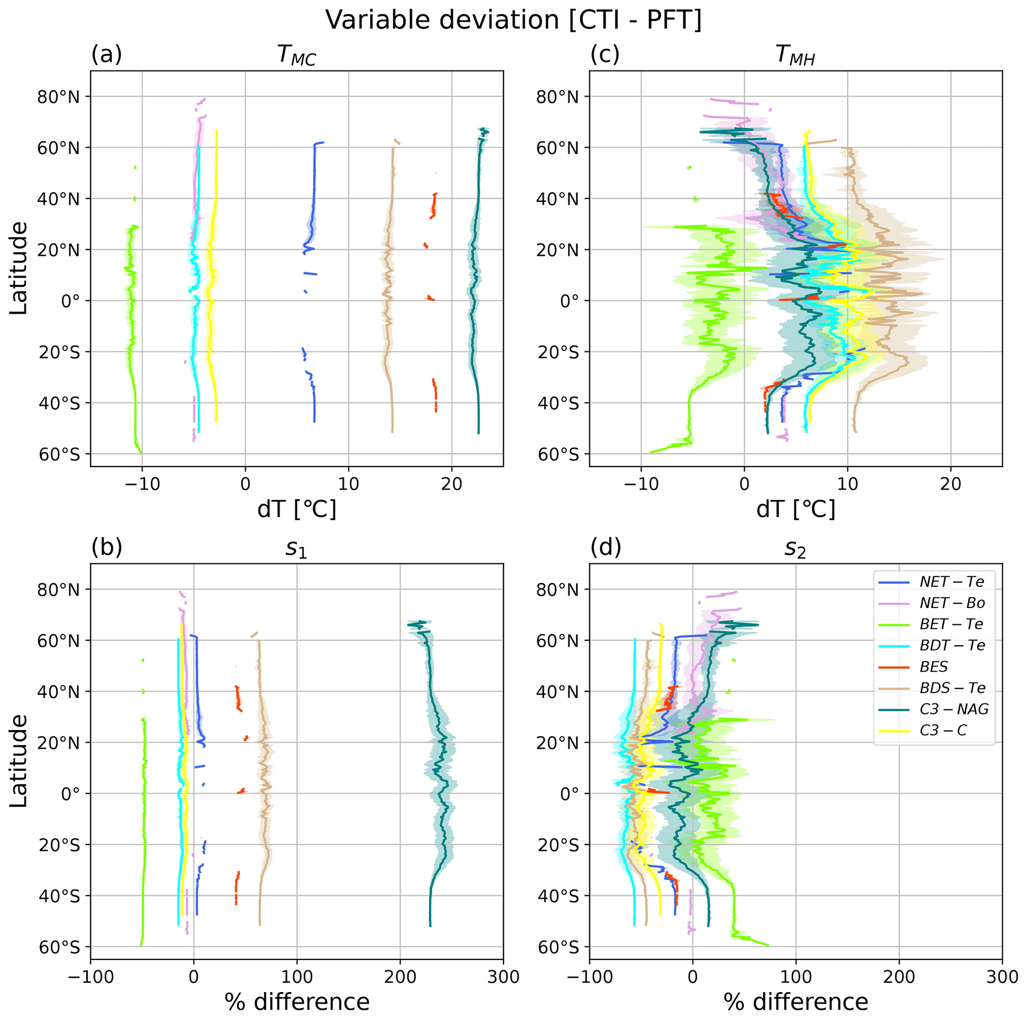
Figure 8 Latitudinal mean and standard deviation (σ) of the difference between CTI-informed and PFT-specific temperature tolerance metrics and resilience parameters of vegetative Φ_PSIImax values, including (a) cold temperature tolerance (T_MC), (b) cold temperature resilience (s₁), (c) hot temperature tolerance (T_MH), and (d) hot temperature resilience (s₂). Here only grid cells having |CTI| values ≤ 900 and targeted PFT cover are included in the calculation of latitudinal mean and standard deviation. Targeted PFTs refer to PFTs in which total covered area within the grid cells having |CTI| ≤ 900 accounts for ≥ 50 % of its global total distribution area. Each PFT-specific result is shown as separate colors, with the shaded regions of the same color being ± 1σ at each latitude.

3.2.3 Spatial distribution of the differences between CTI-informed and PFT-specific parameterizations

To identify specific geographical locations where PFT-specific temperature tolerance or resilience of Φ_PSIImax differed from the CTI-informed counterparts, we calculated the difference in T_MC, T_MH, s₁, and s₂ between CTI-informed and PFT-specific parameterizations at each grid cell. Only PFTs with total cover area within the grid cells of |CTI| ≤ 900 accounting for ≥ 50 % of its global total distribution area were included in this analysis, resulting in the following PFTs: NET-Te, NET-Bo, BET-Te, BDT-Te, BES, BDS-Te, C3-NAG, and C3-C. The latitudinal mean and standard deviation of compared results for all grid cells that contained said PFT were calculated and are shown in Fig. 8.

Our results showed that PFT-specific T_MC for all analyzed PFTs had larger differences compared to the CTI-informed counterparts, but no obvious latitudinal variability was observed, as the magnitude of the variation was about 2 °C. CTI-informed T_MC for BET-Te, NET-Bo, BDT-Te, and C3-C had a value below the corresponding PFT-specific T_MC (stronger cold tolerance) by 11, 5, 5, and 3 °C, respectively, while CTI-informed T_MC for NET-Te, BDS-Te, BES, and C3-NAG had values above the corresponding PFT-specific T_MC (weaker cold tolerance) by around 6–7, 14, 18, and 22–23 °C, respectively (Fig. 8a). Similarly, the differences between CTI-informed and PFT-specific cold resilience metric s₁ showed slight latitudinal variability but differed among different PFTs. The CTI-informed s₁ for C3-NAG was 2 times greater than its PFT-specific counterpart (210 %–250 %), followed by BDS-Te and BES with around 40 %–60 % greater CTI-informed s₁ than its PFT-specific counterpart (Fig. 8b), indicating that CTI-informed Φ_PSIImax values of C3-NAG, BDS-Te, and BES were more resilient to cold temperature than the corresponding PFT-specific estimation. In contrast, CTI-informed Φ_PSIImax values of C3-C, NET-Bo, BDT-Te, and BET-Te became less resilient to cold temperatures than PFT-specific parameterization, with the Φ_PSIImax value of BET-Te having the largest cold resilience reduction (50 %; Fig. 8b). Compared to the PFTs discussed above, there was almost no significant difference in NET-Te between the two parameterizations. Overall, our results indicated that C3-NAG, BES, BDS-Te, and BET-Te were key PFTs with larger changes in cold tolerance (> 10 °C) and cold resilience (> 40 %) of CTI-informed Φ_PSIImax values compared to the corresponding PFT-specific counterparts.

The differences in T_MH and s₂ between CTI-informed and PFT-specific parameterizations for all analyzed PFTs showed larger latitudinal variability compared to their cold temperature counterparts. CTI-informed T_MH for BET-Te was lower (lower hot tolerance) than the PFT-specific T_MH by around 2.5–10 °C with a larger reduction in T_MH observed in southern middle latitudes (Fig. 8c). In contrast, CTI-informed T_MH for BDT-Te, BES, BDS-Te, and C3-C all larger than the PFT-specific counterparts, with the increased T_MH difference between the two parameterizations from high to lower latitude, especially from 25–40° N and S (Fig. 8c). Among these PFTs, CTI-informed T_MH for BDS-Te showed the largest increase with the latitudinal mean values by around 10–17 °C across 60° N–60° S compared to the PFT-specific counterpart. CTI-informed latitudinal mean T_MH for C3-C and BDT-Te increased by 6–12 °C across the covered latitude region compared to the PFT-specific counterpart. Unlike PFTs discussed above, NET-Te, C3-NAG, and NET-Bo had diverging T_MH differences between the two parameterizations across latitudinal gradients. Compared to the PFT-specific counterpart, CTI-informed T_MH for NET-Te showed a maximum 2.5 °C decrease around 60° N but a maximum 10 °C increase around 20° N (Fig. 8c). Similarly, CTI-informed T_MH for C3-NAG and NET-Bo decreased by 5 °C beyond 60° N but increased by around 1–7 °C across 60° N–50° S compared to the corresponding estimation by PFT-specific parameterization (Fig. 8c).

The CTI-informed s₂ indicated that the Φ_PSIImax value of BET-Te should have higher hot resilience than the PFT-specific counterparts on average across all latitude bands, with a wide range of percentage increase (7 %–72 %) across 30° N–60° S. In contrast, BDT-Te, BDS-Te, C3-C, NET-Te, and BES all had lower hot resilience of Φ_PSIImax than the PFT-specific estimation (Fig. 8d). CTI-informed hot resilience of Φ_PSIImax for BDT-Te and BDS-Te decreased by around 45 %–68 % from 60° N–50° S, followed by C3-C, BES, and NET-Te with around a 17 %–52 % decrease in CTI-informed hot resilience of Φ_PSIImax compared to their PFT-specific counterparts (Fig. 8d). CTI-informed s₂ for both NET-Bo and C3-NAG had diverging differences with the corresponding PFT-specific counterparts across latitudinal gradients. In the northern latitudes, the hot temperature resilience parameter T_MH for C3-NAG increased by up to 25 % from 30–60° N and from 30–60° S, spiking to over 50 % beyond 60° N, but decreased from 30° N–30° S compared to the corresponding PFT-specific counterparts. NET-Bo showed no significant difference between CTI-informed and PFT-specific hot resilience estimation in the southern latitudes and around 30–50° N, while it showed up to a 50 % increase in CTI-informed values in around 50–80° N compared to PFT-specific counterparts. In total, these findings indicated that BDS-Te, BET-Te, BDT-Te, and C3-C were PFTs with larger changes in hot tolerance (> 5 °C) and hot resilience (> 10 %) of CTI-informed Φ_PSIImax values compared to the corresponding PFT-specific counterparts. However, the differences in these hot temperature response metrics between the two parameterizations showed large variability across the latitude.

4 Discussion

4.1 PFT variation in the temperature tolerance and resilience of photochemical efficiency

Our study gathered global-scale PAM fluorometry observations to quantify temperature regulation on Φ_PSIImax values of 12 PFTs. The developed PFT-specific rectangular functions can capture the optimal Φ_PSIImax value of 0.8 within different ranges of temperature and the decrease in Φ_PSIImax in each PFT with colder and hotter temperatures (Fig. 3). The variability in Φ_PSIImax around the ideal temperature range echoed observed variability across species in response to similar conditions (Li et al., 2004). Few previous studies (Sastry and Barua, 2017; Slot et al., 2019; Perez and Feeley, 2020; Tiwari et al., 2021; Kunert et al., 2022) utilized different functions to fit this heat response of Φ_PSIImax values to the warming climate. These studies mainly focused on specific species, such as tropical evergreen and deciduous species. To our knowledge, our study is the first global-scale effort that quantifies the differences in this temperature–Φ_PSIImax relationship among 12 general PFTs. The generated PFT-specific temperature–Φ_PSIImax functions can be directly applied to adjust the Φ_PSIImax parameter for simulating temperature feedback of photosynthetic energy partitioning in terrestrial ecosystem models (TEMs) and Earth system models (ESMs).

One advantage of the developed temperature–Φ_PSIImax model is its capability for quantifying the temperature tolerance and resilience of Φ_PSIImax values and assessing their differences among different PFTs. Our results highlighted the trade-off scheme of temperature responses of the various PFTs' Φ_PSIImax values, in which the more temperature-resilient PFTs were less temperature tolerant, and vice versa (Fig. 4). Our finding was consistent with previous studies (Tiwari et al., 2021; Kunert et al., 2022) that also found a negative relationship between temperature tolerance and resilience metrics for some tropical tree species, although the definition of temperature tolerance and resilience metrics in Tiwari et al.'s (2021) study was not completely consistent with our definition. This trade-off may be associated with the selection of different PFTs' protection strategies under current and historical temperature stress. Temperature-resilient PFTs may protect PSII from damage via NPQ mechanisms, such as heat shock proteins (HSPs) and the xanthophyll cycle (Adams and Demmig-Adams, 1994; Verhoeven et al., 1999; Wahid et al., 2007). Temperature-tolerant PFTs may have more flexibility when it comes to PSII protections due to either phenological responses (i.e., leaf senescence under cold/hot stress, maximizing warm-season growth; Sakai, 1980) or physiological feedback (i.e., evapotranspiration cooling under hot stress; Havaux, 1992).

According to this trade-off between temperature tolerance and resilience of the PFTs' Φ_PSIImax temperature response, we identified the PFT group with cold and hot temperature tolerance (BES and C3-NAG), the PFT group with cold and hot temperature resilience (BDT-Te, NET-Bo, C4-G, C3-C), and the temperature specialist PFT group (BET-Te, BDT-Tr, BET-Tr, C4-C, and BDS-Te). NET-Te adopted a generalist strategy, with tolerance and resilience values near the mean across PFTs, though this may be an inherent bias in the datasets. The higher tolerance of C3-NAG to both cold and hot temperatures was probably associated with its discrete distribution across diverse habitats, such as the Amazon and boreal regions (Ke et al., 2012). Long-term exposure to diverse temperatures has evolved diverse C3-NAG species and cultivars, which have distinct abilities to suppress oxidative stress under temperature stress and therefore a broad heat and cold tolerance of Φ_PSIImax (Soliman et al., 2012; Filho et al., 2018). Similarly, BES, which was usually distributed in the Mediterranean climate with typical cold winter and drought summer (Ke et al., 2012), had been found to maintain higher photochemical yields under hot and cold temperatures by adjusting vegetation structure and decreasing chlorophyll content (Oliveira, 2000). BDT-Te was the PFT with the most heat resilience, reflecting a strong HSP and stomatal conductance response (Solhaug and Haugen, 1998; Wittmann and Pfanz, 2007; Song et al., 2014). Some species within BDT-Te had a phenotypic abscission response to high temperature (Shirke and Pathre, 2003), which may be a reason behind the mild variability in Φ_PSIImax measurements at high temperature (Fig. 3f). The higher cold and hot temperature resilience of C3-C may be related to crop engineering selection of crop genotypes that can be more resilient to extreme temperature and weather events (Basu et al., 2009; Molina-Bravo et al., 2011; Zhou et al., 2015; Sharma et al., 2017). In the temperature specialist PFT group, BET-Te was the PFT with the strongest hot tolerance and strongest cold resilience, which may be due to its adaptation to hot temperatures by having a phenological mechanism with year-round leaf turnover (Williams-Linera, 1997) and having freezing resistance in leaves (Sakai, 1980). Similar to BET-Te, BDT-Tr could maintain higher Φ_PSIImax at temperatures up to 42 °C. The high heat tolerance of BDT-Tr was consistent with Tiwari et al. (2021) and was probably associated with the synthesis of HSPs under long-term exposure to tropical high temperature (Taleisnik and Grunherg, 1994).

Our definitions of temperature tolerance and resilience are not completely the same as previous studies; however, they can be comparable after conversion. For example, previous studies (Tiwari et al., 2021; Kunert et al., 2022) estimated T₅₀ as the same definition of m₂ in our PFT-specific temperature–Φ_PSIImax model (Eq. 1) but quantified temperature resilience of Φ_PSIImax as decline width (DW = T₉₅ − T₅) and temperature tolerance of Φ_PSIImax as T₅. Here T₅ and T₉₅ referred to the temperature at which Φ_PSIImax declined with temperature change by 5 % and 95 %. By calculating T₅₀, T₉₅, and T₅ using the fitted Eq. (1), we found that the parameterization for BET-Tr using our model resulted in T₅ of 42.35 °C, T₅₀ of 49.98 °C, and a resilience metric (T₉₅ – T₅) of 15.26 °C. This result was close to Tiwari et al. (2021) estimations of dry (wet) season T₅ = 43.5 °C (41.9 °C), T₅₀ = 51.6 °C (49.4 °C), and T₉₅ – T₅ = 16.6 °C (15.4 °C) averaged across diverse BET-Tr species. Also, our estimations of T₅, T₅₀, and T₉₅ values for NET-Te were 38.7 °C, 46.7 °C, and 54.7 °C, respectively. The estimated T₅ and T₉₅ fell within the Kunert et al. (2022) estimated span of the six NET-Te species' for T₅ (38.5–43.1 °C) and T₉₅ (53.9–57.5 °C). However, the estimated T₅₀ was somewhat lower than the corresponding estimation of 47.8–52.3 °C by Kunert et al. (2022).

4.2 Climatology-driven convergent temperature–Φ_PSIImax response across PFTs in a certain region

The formation and application of the CTI as an integrated indicator of climatological annual mean temperature, winter median temperature, and summer median temperature allowed for quantifying the variation in temperature tolerance and resilience of photochemical efficiency with climatological gradients. This CTI-incorporated temperature–Φ_PSIImax parameterization (Fig. D2) was comparable with the corresponding PFT-informed temperature–Φ_PSIImax parameterization within the region of |CTI| < 150 and increased predictive power within the region with 150 ≤ |CTI| ≤ 900, implying that the irreversible variability in photochemical efficiency of a plant with temperature change mainly depends on its acclimation and adaptation to climatology in these regions. PFT has been widely applied to interpret the variation among plants in physiological, morphological, and phenological traits and correlated to plant adaptation to local environmental conditions and to plant resource capture and survival strategies (Reich et al., 2003; Kelly et al., 2021). However, our results demonstrated that the temperature sensitivity and tolerances of photochemical efficiency trait in a certain CTI band (|CTI| ≤ 900) are convergent and can be parameterized using a CTI-informed fundamental function. This universal function can be directly incorporated into TEMs and ESMs to parameterize the temperature feedback of photosynthetic light reactions instead of using PFT-specific parameterization, which requires more parameters. Our finding was similar to the study of Heskel et al. (2016) that found consistent temperature sensitivity of leaf respiration across several PFTs and biomes and parameterized it using a universal temperature-dependent function. The convergent temperature responses of these plant traits may reflect the occurrence of phenotypic plasticity or ecotypic variations as a result of plant acclimation and adaptation to its inhabited climatological temperature (Berg et al., 2010; Marias et al., 2016) or universal metabolic constraints on vegetation temperature feedback (Heskel et al., 2016).

The global distribution of the regions within the bounds of improved prediction (150 ≤ |CTI| ≤ 900) were concentrated around subtropical regions (30–40° N and S) and along the transition zones from the mid-latitudes to the polar regions (50–70° N and 50–60° S) (Fig. 5a and b). These regions typically had a large inter-seasonal variability in temperature or contrasting precipitation seasonality coupling with hot temperature through the year. Several observations (Wahid et al., 2007; Li et al., 2008; Soliman et al., 2012; Marias et al., 2016) have shown that plant species in a variable climatological environment have been more phenotypically plastic and representative of “experienced temperature” through different feedback. Such feedback examples include synthesis of non-structural carbon under temperature stress, generation of HSP to avoid heat damage, and increasing evaporative cooling through adjusting stomatal size and density. Moreover, moisture stress may modulate plant plastic capacity due in part to an attempt to maximize water use efficiency (WUE) and maintain homeostasis (Wahid et al., 2007; Lin et al., 2015; Marias et al., 2016). The improved prediction of temperature–Φ_PSIImax relationships in these regions by our CTI-informed parameterization was consistent with previous observations in the subtropical region in that species from contrasting climate of origin (desert vs. coastal) did not show significantly different tolerance when growing in the common environment (Knight and Ackerly, 2001).

4.3 The correlation of temperature tolerance and resilience of photochemical efficiency with its local habitat climatology

Our results indicated that Φ_PSIImax tends to be less cold tolerant and resilient but less hot tolerant and more hot resilient along warm-to-cold climatological gradients, except for the temperature region across 40–50° N and 40–60° S. The decrease in both cold tolerance and resilience of photochemical efficiency along warm-to-cold climatology was probably because more extreme and highly frequent cold temperature (e.g., chilling) in colder regions may damage metabolic processes and inhibit adaptive vegetation feedback, such as sugar synthesis, osmotic production, and pigment synthesis (Hajihashemi et al., 2018), or induce initiation of NPQ to dissipate the resulting excess energy (Rapacz et al., 2004). In contrast, our finding of the decrease in hot tolerance along warm-to-cold climatology supported previous conclusions that vegetation distributed in warmer climates have greater heat tolerance (Smillie and Nott, 1979; Salvucci and Crafts-Brandner, 2004; Marias et al., 2016; Fadrique et al., 2022). The lack of a latitudinal trend of temperature tolerance and resilience across 40–50° N and 40–60° S was probably due to the highly variable climatology in the mid-latitudes. Therefore, the temperature tolerance and resilience of Φ_PSIImax may reflect local climate properties.

4.4 The advantage of CTI-informed parameterization over PFT-specific parameterization is PFT dependent

Our results suggested that the importance of climatological regulation on temperature–Φ_PSIImax relationships differs among different PFTs. In the region with comparable or improved prediction power by CTI-informed parameterization, CTI-informed Φ_PSIImax values of C3-NAG, BES, BDS-Te, and BET-Te showed larger changes in cold tolerance (> 10 °C) and cold resilience (> 40 %) compared to the corresponding PFT-specific counterparts, whereas CTI-informed Φ_PSIImax values of BDS-Te, BET-Te, BDT-Te, and C3-C had larger changes in hot tolerance (> 5 °C) and hot resilience (> 10 %) compared to the corresponding PFT-specific counterparts. As discussed in Sect. 4.2, this result may reflect the acclimation and adaptation of these PFTs to local temperature variability instead of the PFT-unified life history strategy (Curtis, 2016). For example, C3-NAG and BES are distributed across wide latitude ranges, 67.5° N–52° S and 52° N–43.5° S, respectively, with diverse climatological variability in distribution space, whereas BDS-Te and BET-Te were mainly distributed in temperate regions with a large seasonal variability in temperature (Lawrence and Chase, 2007; Ke et al., 2012; Lawrence et al., 2019).

4.5 Uncertainty and future work

Fully identifying the underlying mechanisms of why Φ_PSIImax declines with temperature is beyond the scope of this study; however they likely fall into two categories: photophysical effects and biophysiochemical effects. From the photophysical perspective, as temperature changes outside of an idealized range, sustained NPQ is known to increase in some plants (Porcar-Castell, 2011), though the variation in the experimental method across the gathered studies in this dataset makes the temporal scale of sustained NPQ accumulation inconsistent. A less straightforward photophysical phenomena is how the maximum and minimum dark-adapted fluorescence yields individually respond to temperature, which would describe a separation of sustained NPQ and photoinhibited reaction centers (i.e., qL is less than 1 even when leaves are fully dark-adapted). This separation is also connected to state transitions between PSII and PSI (Baker et al., 2007; Rath et al., 2022). Biophysiochemical effects are tied to changes that may be informed by WUE strategies or damage to leaf cellular integrity (Kadir et al., 2006), as well as membrane and enzyme degradation (Schrader et al., 2004). In principle, there would be both a hot and cold temperature beyond which intra-cellular mechanisms break down, bringing Φ_PSIImax to zero, though they likely vary with life strategy and phenology (i.e., evergreen needleleaf in cold temperatures; Corcuera et al., 2011). In future work, findings along this line would provide physically justified bounds on allowed parameter values, preventing features like the cold temperature result of BET-Te (Fig. 3d).

The PFT-informed parameterizations of Φ_PSIImax responses to temperature were able to demonstrate a trade-off strategy of temperature tolerance and resilience of Φ_PSIImax values among 12 commonly used PFTs in TEMs and ESMs. However, the 4 PFTs of the original 16 that did not have sufficient data to be described were all boreal plants: needleleaf deciduous boreal tree (NDT-Bo), broadleaf deciduous boreal tree (BDT-Bo), broadleaf deciduous boreal shrub (BDS-Bo), and C3 Arctic grass (C3-AG). Since the boreal region is expected to experience more extreme temperature and climate events (Francis and Vavrus, 2015), understanding how boreal ecosystems respond to changing temperatures becomes more important and needs to be addressed in the future. Among the 12 parameterized PFTs, C4 crops were underrepresented in terms of data and also need to be further studied. Moreover, considering the number of diverse crop species and increased engineering selection of crop genotypes (Leister, 2022), future studies need to better investigate species- and genotype-specific temperature tolerances and resiliencies of photochemical efficiency for main food and commercial crops.

The CTI-informed parameterization of Φ_PSIImax responses to temperature was limited by the distribution of the original field site sub-datasets' geographic distribution, which were concentrated in the mid-latitudes and had little data in the highly productive tropical and boreal forest regions. This data limitation resulted in uncertainty in the assessment of the predictive power of CTI-informed parameterization in the tropical and boreal forest regions. This uncertainty can be addressed in the future with new datasets to allow for more robustly parameterized CTI-informed temperature–Φ_PSIImax relationships in these regions.

A potential complication in comparing the PFT-specific and CTI-informed parameterization is a difference in the temperature regimes under which data were collected. The data used in the PFT-specific results include plants growing in greenhouses lacking experienced climatological variation, such that this initial “shock” towards homeostasis may be dealt with using mostly quick-reacting methods such as energy-dependent NPQ, as no previous temperature acclimation had been required. As plants acclimate to a specific climatology, they shift from reversible to irreversible photoinhibitory strategies, primarily sustained NPQ (Rizza et al., 2001; Rapacz et al., 2004; Ehlert and Hincha, 2008). Future comparison between the two parameterizations calls for a more consistent and extensive dataset covered by diverse plant species/PFTs under diverse natural habitats.

A broader application of this methodology to other energy partitioning pathways of light reactions is required to fully link light use efficiency with GPP (Gu et al., 2019). Φ_PSIImax (Fv$/$Fm) is a ratio composed of the minimum and maximum levels of chlorophyll fluorescence from a dark-adapted leaf (Tietz et al., 2017). In future work, we will further isolate the temperature-dependent changes between these two variables and link the derived temperature–Φ_PSIImax functions in this study with the estimation of relative light saturation and rates of other energy dissipation pathways. These future efforts will allow clarification if the decline in Φ_PSIImax is due to a rise in energy-independent NPQ or a change in the availability of PSII reaction centers for photochemistry. There was an indication within the dataset that the length of temperature exposure also affects the temperature–Φ_PSIImax response, which requires further examination. The connected dynamics of water and heat stress have been examined (Ogaya et al., 2011; Ashraf and Harris, 2013; Seng et al., 2023; Sommer et al., 2023), but extensive PFT-specific relationships and climatological impacts need to be explored in the future.

5 Conclusion

The decline in Φ_PSIImax outside of an ideal temperature range is a consistent response across 146 species covering diverse climatological conditions. We introduce a model to describe this temperature response with easily interpretable parameters.

There was variability in both the range of temperatures under which PFTs maintained a maximum Φ_PSIImax (tolerance) and the rate of decline outside of the range (resilience). More temperature-resilient PFTs were less temperature tolerant, and vice versa.

Temperature responses along the tolerance–resilience trade-off suggest three categories of life history strategies of light partitioning to hot and cold extremes: the PFTs with cold and hot temperature tolerance (BES and C3-NAG), the PFTs with cold and hot temperature resilience (BDT-Te, NET-Bo, C4-G, and C3-C), and the temperature specialist PFT group (BET-Te, BDT-Tr, BET-Tr, C4-C, and BDS-Te).

Indices of climatological temperature variability in space were found to explain some of the variations not captured in the PFT-specific parameterizations of the temperature–Φ_PSIImax relationship alone. We leveraged this into a climatology-informed CTI scheme that was able to improve predictive power in certain regions compared to the PFT-specific schemes.

The global distribution of CTIs suggests that the regions in which the CTI-informed parameterization performs better compared to the PFT-specific parameterizations fall in the transition zones from temperate to tropical regions and from the mid-latitudes to the polar region. This is likely tied to the more variable climatological environment experienced in the regions, promoting a more consistent community temperature response via acclimation.

The advantage of CTI-informed parameterization over PFT-specific parameterizations is PFT-dependent and varies across latitudes. Climatological regulation on the temperature feedback of Φ_PSIImax is critical for PFTs with broad distributions in diverse habitats or those living in local regions with a large seasonal variability in temperature.

Appendix A: Monte Carlo scheme for determining parameter constraints in the fitting function

Differences in available data within each PFT-specific sub-dataset may induce uncertainty in estimated parameters in Eq. (1) and make the fitted parameter for each PFT-specific temperature response function of Φ_PSIImax incomparable. To avoid this parameterization uncertainty, we imposed unified constraints on each parameter's range using a Monte Carlo scheme. We performed three tests. First, we did a test that involved dividing all paired Φ_PSIImax and temperature data within the dataset of each PFT into eight subsets. Each subset covers a 10° range of measured temperature beginning at −17 °C. Each subset then underwent a permutation, with a percentage of the subset's data selected randomly. Each random group of Φ_PSIImax and temperature measurements in a PFT-specific subset was aggregated and fitted to the model (Eq. 1), and the parameters were recorded. The permutation, random selection, and function fitting were all repeated for 700 iterations. This Monte Carlo scheme was done with three different percentages (75 %, 50 %, 33 %) of data taken from the PFT-specific subsets to observe the sensitivity of the fitting results to the amount of fitted data. The estimated parameter values from 2100 instances of fitting were finally integrated to describe the distribution range of each parameter. The parameter constraints within the range between the mean of each parameter ± 2σ, here σ referring to the standard deviation of each parameter's distribution, were recorded. This gave a view of what a parameterization with wide temperature ranges may produce but could be heavily biased by the most extreme subsets with limited data.

For the second test, a similar process was performed, except there were three subsets capturing the relatively constant central temperature range [7–35 °C] and the outer decline in cold and hot temperatures. A total of 10 % of each subdivision's data was selected to produce aggregated data for fitting Eq. (1) containing the same number of data points as the average PFT-specific sub-dataset. A total of 2000 iterations of aggregated data points were modeled to produce ranges of parameters that had less chance of being biased by the most extreme data points. However, there was a spreading of modeled values to the point of being unphysical in their interpretation, likely due to aggregated data points that did not actually have cohesive temperature–Φ_PSIImax dynamics.

The third test analyzed the distribution of temperature–Φ_PSIImax data pairs with Φ_PSIImax around $a/\mathrm{2}$. The spread of temperature values around this boundary serves as the bounds implicit in the dataset itself and proved to be more physically realistic. By comparing the minimum and maximum temperature values of the $a/\mathrm{2}{\mathrm{\Phi }}_{\text{PSIImax}}$ data points in cold and hot temperature extremes to the parameter distributions in the previous tests, the parameter space in Table A1 was chosen.

Table A1 Constrained range of fitted parameters using the Monte Carlo scheme.

Appendix B: Methodology for performing the aligned rank transform

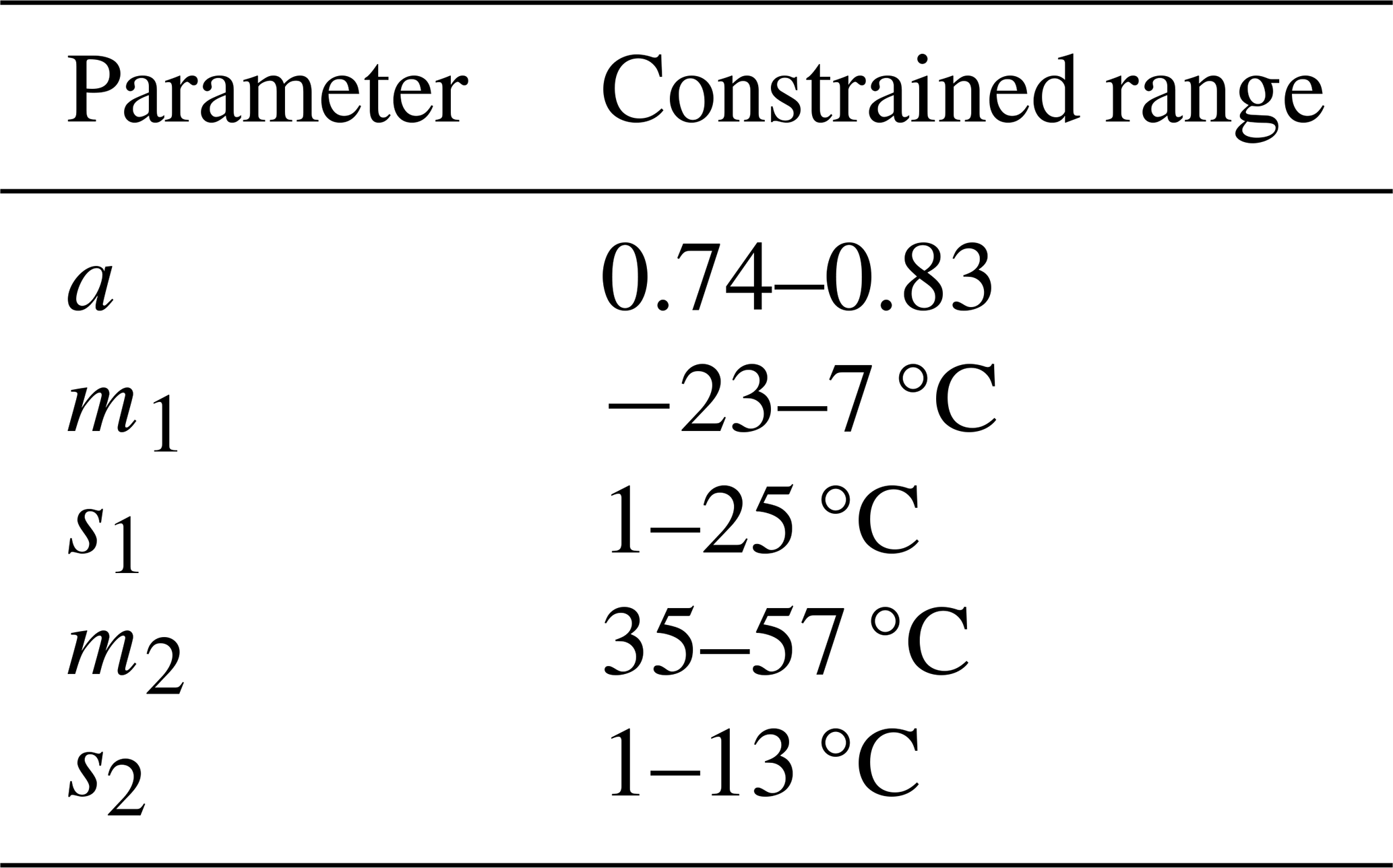
We performed ANOVA to evaluate how climatology metrics affect the prediction efficiency of the developed PFT-specific temperature–Φ_PSIImax function. Before assigning ranks and performing the standard ANOVA analysis, we performed several preprocessing steps that isolated each interaction term between SMET, WMET, and AAT. First, the aligned X values for the main effect of SMET, WMET, and AAT were found using Eqs. (B1)–(B3).

$$\begin{array}{}\text{(B1)}& {\displaystyle }& {\displaystyle }{\text{SMET}}^{\prime }=(X-Y_{ijk})+\left(\stackrel{\mathrm{‾}}{{\text{SMET}}_i}-\mathit{\mu }\right)\text{(B2)}& {\displaystyle }& {\displaystyle }{\text{WMET}}^{\prime }=(X-Y_{ijk})+\left(\stackrel{\mathrm{‾}}{{\text{WMET}}_j}-\mathit{\mu }\right)\text{(B3)}& {\displaystyle }& {\displaystyle }{\text{AAT}}^{\prime }=(X-Y_{ijk})+\left(\stackrel{\mathrm{‾}}{{\text{AAT}}_k}-\mathit{\mu }\right)\end{array}$$

Here Y_ijk is the “cell mean”, calculated as the mean of all X values in the test as the ith level of SMET, the jth level of WMET, and the kth level of AAT as found using Eq. (6). The μ is the mean of all X values used in the test. $\stackrel{\mathrm{‾}}{{\text{SMET}}_i}$, $\stackrel{\mathrm{‾}}{{\text{WMET}}_j}$, and $\stackrel{\mathrm{‾}}{{\text{AAT}}_k}$ are the mean value of X at the given level of SMET, WMET, and AAT, respectively.

The aligned X values for the two-way effects of SMET, WMET, and AAT were found using Eqs. (B4)–(B6).

$$\begin{array}{}\text{(B4)}& {\displaystyle }\begin{array}{rl}{\text{SMET}}^{\prime }\times {\text{WMET}}^{\prime }=& (X-Y_{ijk})+(\stackrel{\mathrm{‾}}{{\text{SMET}}_i{\text{WMET}}_j}\\ & -\stackrel{\mathrm{‾}}{{\text{SMET}}_i}-\stackrel{\mathrm{‾}}{{\text{WMET}}_j}+\mathit{\mu })\end{array}\text{(B5)}& {\displaystyle }\begin{array}{rl}{\text{SMET}}^{\prime }\times {\text{AAT}}^{\prime }=& (X-Y_{ijk})+(\stackrel{\mathrm{‾}}{{\text{SMET}}_i{\text{AAT}}_k}\\ & -\stackrel{\mathrm{‾}}{{\text{SMET}}_i}-\stackrel{\mathrm{‾}}{{\text{AAT}}_k}+\mathit{\mu })\end{array}\text{(B6)}& {\displaystyle }\begin{array}{rl}{\text{WMET}}^{\prime }\times {\text{AAT}}^{\prime }=& (X-Y_{ijk})+(\stackrel{\mathrm{‾}}{{\text{WMET}}_j{\text{AAT}}_k}\\ & -\stackrel{\mathrm{‾}}{{\text{WMET}}_j}-\stackrel{\mathrm{‾}}{{\text{AAT}}_k}+\mathit{\mu })\end{array}\end{array}$$

The aligned X values for the three-way interaction were found using Eq. (B7).

$$\begin{array}{}\text{(B7)}& \begin{array}{rl}& {\text{SMET}}^{\prime }\times {\text{WMET}}^{\prime }\times {\text{AAT}}^{\prime }=(X-Y_{ijk})\\ & +(\stackrel{\mathrm{‾}}{{\text{SMET}}_i{\text{WMET}}_j{\text{AAT}}_k}-\stackrel{\mathrm{‾}}{{\text{SMET}}_i{\text{WMET}}_j}\\ & -\stackrel{\mathrm{‾}}{{\text{SMET}}_i{\text{AAT}}_k}-\stackrel{\mathrm{‾}}{{\text{WMET}}_j{\text{AAT}}_k}+\stackrel{\mathrm{‾}}{{\text{SMET}}_i}\\ & +\stackrel{\mathrm{‾}}{{\text{WMET}}_j}+\stackrel{\mathrm{‾}}{{\text{AAT}}_k}-\mathit{\mu })\end{array}\end{array}$$

$\stackrel{\mathrm{‾}}{{\text{SMET}}_i{\text{WMET}}_j}$ is the mean value of X at the ith level of SMET and jth level of WMET. $\stackrel{\mathrm{‾}}{{\text{SMET}}_i{\text{AAT}}_k}$ is the mean value of X at the ith level of SMET and kth level of AAT, and $\stackrel{\mathrm{‾}}{{\text{WMET}}_j{\text{AAT}}_k}$ denotes the mean value of X at the jth level of WMET and kth level of SMET. The term $\stackrel{\mathrm{‾}}{{\text{SMET}}_i{\text{WMET}}_j{\text{AAT}}_k}$ is equivalent to the “cell mean”. These terms were then used to perform the standard ANOVA analysis.

Appendix C: Algorithm for smoothing fitted parameters and corresponding central CTI values of QSA sets

To decrease the existence of noisy data impact on the regression of fitted parameters on the central CTI values of QSA sets, we smoothed the fitted parameters and corresponding central CTI values of the QSA sets before performing the final regression analysis. To determine a smoothing window width, we defined the “distance” between two QSA sets as the difference between their central CTI values, then integrated all distances between all combinations of QSA sets to determine their histogram distribution (Fig. C1). The median CTI value of this distribution, hereafter referred to as the median intra-point distance (MID), was 367; it was then used as the smoothing window width around a central CTI value q. Each individual QSA set-fitted parameter (m₁, m₂, s₁, s₂) from Eq. (1) was then adjusted to the mean of the corresponding parameter estimates within q ± MID.

Figure C1 CDF of the distances between central CTI values of the QSA sets.

Appendix D: The contribution of climatology temperature metrics and derived CTI to prediction residues by the PFT-specific temperature–Φ_PSIImax functions

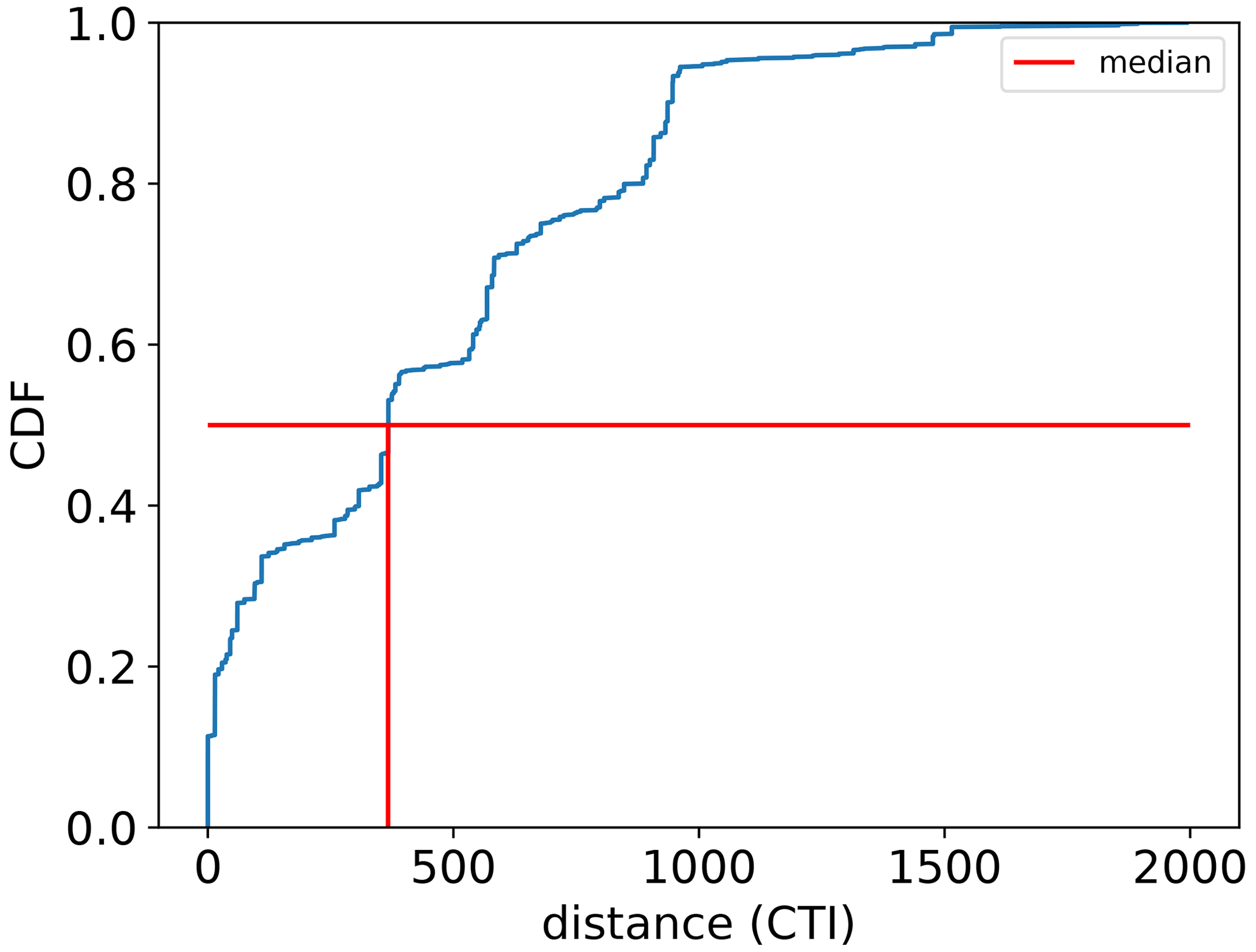
There were consistent results between the ART ANOVA analysis for prediction residues estimated by the PFT-specific temperature–Φ_PSIImax functions (ANOVA_{RS_pft}) and the general temperature–Φ_PSIImax function that resulted from fitting all data within the field site sub-dataset (ANOVA_{RS_gen}) (Fig. D1). The ANOVA_{RS_gen} analysis showed that around 94 % of variances in prediction residues by the PFT-specific temperature–Φ_PSIImax functions were able to be attributed to three climatological temperature metrics (WMET, SMET, and AAT) and their cross terms. The interaction of WMET, SMET, and AAT showed the largest impact and explained around 37 % of variations in prediction residues, followed by the cross effect of WMET and AAT with around 20 % of variations in prediction residues associated with it (Fig. D1). In addition, the cross effect of SMET and WMET and the cross effect of SMET and AAT explained a similar number (around 10 %) of variations in prediction residues. Compared to the cross effect of three metrics, the main effects of individual metrics were relatively lower, with 8.78 %, 6.42 %, and 1.28 % of variations in prediction residues associated with WMET, AAT, and SMET, respectively (Fig. D1). Similar to ANOVA_{RS_gen} analysis, the ANOVA_{RS_pft} analysis indicated that WMET, SMET, and AAT, as well as their interactions, explained 96 % of variances in prediction residues by the PFT-specific temperature Φ_PSIImax function (Fig. D1).

This consistency justified that the regulation of climatological temperature on the temperature–Φ_PSIImax relationship can be estimated using the results of either version of ANOVA. Here we will use the results from ANOVA_{RS_pft}. The outsized difference in the amount of variance associated with the interaction and cross effects of three temperature metrics compared to the main effect of individual metrics suggested that annual mean temperature, together with the winter and summer temperature that the plants usually experienced in their habitats, determined the temperature response of plant photosynthetic light partitioning. Therefore, it was necessary to integrate three climatological temperature metrics to investigate the regulation of climatological temperature on the tolerance and resilience of Φ_PSIImax to climate change. We employed AAT, WMET, SMET, and their interactions to develop a climatology temperature index (CTI) and CTI-informed parameterization of m₁, m₂, s₁, and s₂ from Eq. (1). By substituting observation temperature and site-specific CTI within the field site sub-dataset into CTI-informed and PFT-specific parameterizations, we showed that utilizing the CTI-informed parameterization improved the accuracy of Φ_PSIImax prediction by 4.3 % on average, but this improvement was achieved across the range 150 ≤ |CTI| ≤ 900 (Fig. D2). This range represents the transition away from the mean state of SMET, WMET, and AAT for the field site sub-dataset. For |CTI| below 150, the improvement in the sum of residuals was not significant, implying that CTI-informed temperature dependence of Φ_PSIImax agreed with the PFT-specific results in aggregate.

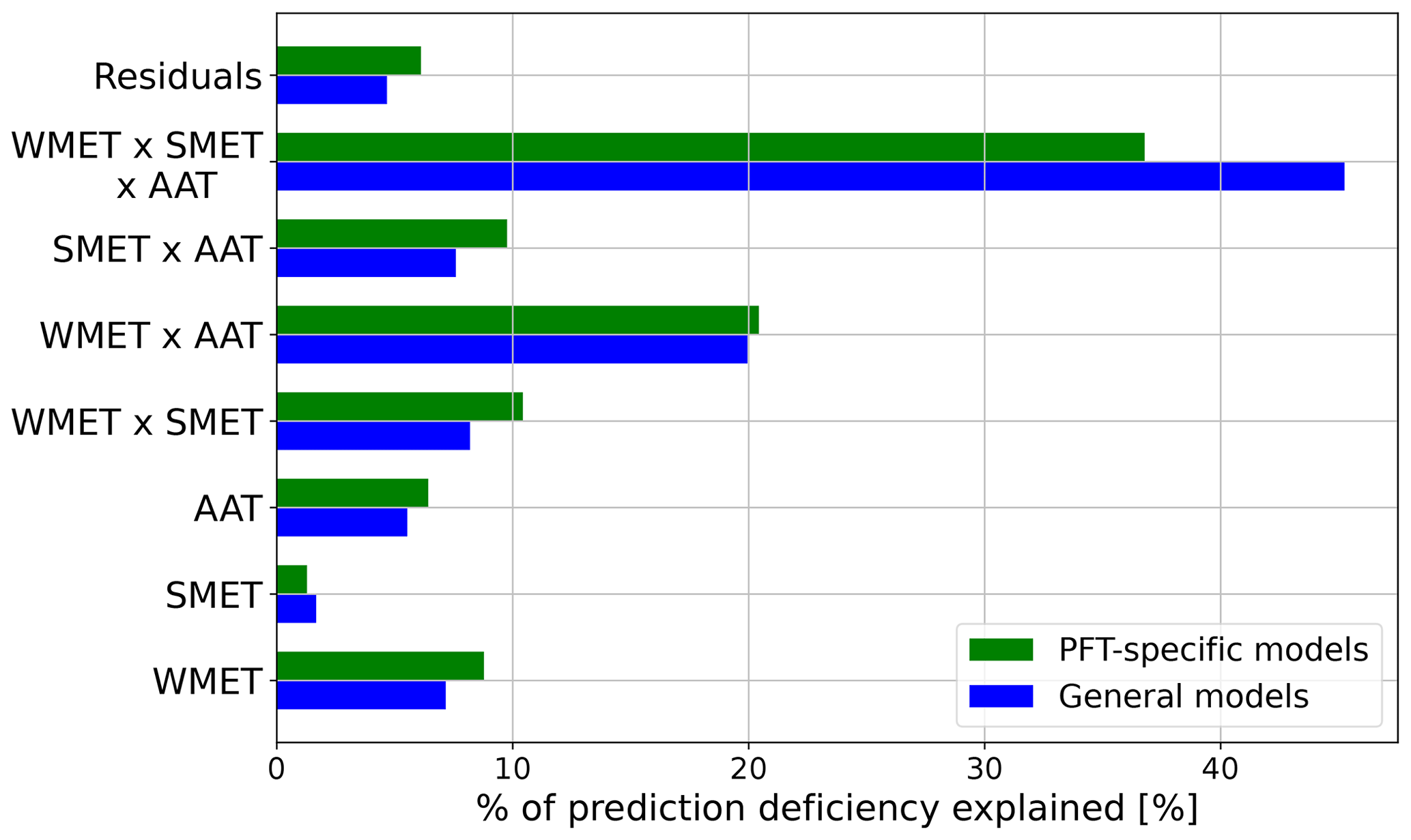
Figure D1 Results comparison of two ART ANOVA analyses. ANOVA_{RS_pft} refers to results from ART ANOVA using prediction residuals from PFT-specific temperature–Φ_PSIImax functions. ANOVA_{RS_gen} refers to results from ART ANOVA using prediction residuals from the general (non-PFT-specific) temperature–Φ_PSIImax function. Here WMET and SMET refer to the median experienced temperature in the winter and summer, respectively, while AAT refers to the annual average temperature.

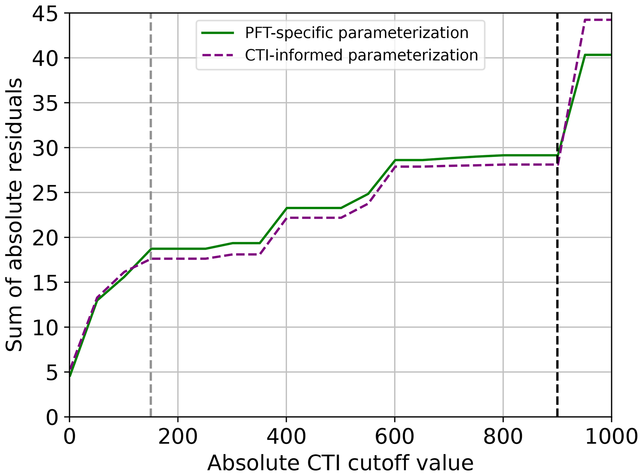
Figure D2 Comparing the sum of the magnitude of the prediction residuals between CTI-informed and PFT-specific parameterization of vegetative temperature–Φ_PSIImax relationship.