Soil carbon-concentration and carbon-climate feedbacks in CMIP6 Earth system models

Achieving climate targets requires mitigation against climate change but also understanding of the response of land and ocean carbon systems. In this context, global soil carbon stocks and their response to environmental changes are key. This paper quantifies the global soil carbon feedbacks due to changes in atmospheric CO₂, and the associated climate changes, for Earth system models (ESMs) in CMIP6. A standard approach is used to calculate carbon cycle feedbacks, defined here as soil carbon-concentration (β_s) and carbon-climate (γ_s) feedback parameters, which are also broken down into processes which drive soil carbon change. The sensitivity to CO₂ is shown to dominate soil carbon changes at least up to a doubling of atmospheric CO₂. However, the sensitivity of soil carbon to climate change is found to become an increasingly important source of uncertainty under higher atmospheric CO₂ concentrations.

1 Introduction

Global soil carbon stocks contain at least twice as much carbon than is stored in the world's vegetation, making soils the largest active store of carbon on the land surface of Earth (Canadell et al., 2021). In the absence of human disturbance and land-use change (Jones et al., 2018), future changes in soil carbon depend on the sensitivity to increases in atmospheric CO₂ concentrations and the sensitivity to the associated impacts, such as increases in atmospheric temperatures and changes in precipitation patterns (Varney et al., 2023; Todd-Brown et al., 2014). The quantification of such carbon cycle feedbacks is required to determine the overall response of the climate system to given anthropogenic CO₂ emissions and to help achieve Paris Agreement targets (Friedlingstein et al., 2022; Gregory et al., 2009).

Previous studies have defined land carbon cycle feedbacks within Earth system models (ESMs) from both CMIP6 and CMIP5 ensembles (Arora et al., 2020, 2013). In general, the overall response of carbon stores is separated into those due to changes in atmospheric CO₂ (ΔCO₂) and those due to changes in global temperature (ΔT), with the latter assumed to represent the overall impacts of climate change on large spatial scales. These components of land carbon cycle feedbacks are called carbon-concentration feedbacks (β_L) and carbon-climate feedbacks (γ_L), respectively (Friedlingstein et al., 2003, 2006). An advantage of using this formulation is that it allows for the quantification of the feedbacks for a given atmospheric CO₂ concentration, which can then be used as a simplified measure to compare amongst ESMs despite the increasing model complexities (Arora et al., 2020, 2013; Gregory et al., 2009). For example, it provides a consistent metric to measure land carbon feedbacks despite the differing climate sensitivities amongst ESMs (Boer and Arora, 2013).

In this study, soil-carbon-driven feedbacks in ESMs are quantified using this βγ formulation (Friedlingstein et al., 2006). Additionally, the βγ formulation is combined with the Varney et al. (2023) framework, which breaks down future changes in soil carbon (ΔC_s) into individual processes which drive this response. This paper makes use of the latest generation of the Coupled Model Intercomparison Project (CMIP6) used within the Intergovernmental Panel on Climate Change 6th Assessment Report (IPCC AR6; IPCC, 2021; Eyring et al., 2016). To do this, soil carbon-concentration and carbon-climate feedback parameters are presented for CMIP6 ESMs, named β_s and γ_s, respectively, together with components which make up β_s and γ_s due to associated processes. The aim of this paper is to (1) quantify the sensitivity of soil carbon to increased atmospheric CO₂ concentrations and associated climate impacts by calculating β_s and γ_s for CMIP6 ESMs, (2) investigate the linearity of future soil carbon change at higher levels of atmospheric CO₂ increase, and (3) identify the fraction of the land carbon response to climate change that is due to global soils.

2 Methods

2.1 C4MIP simulations

The Coupled Climate-Carbon Cycle Model Intercomparison Project (C4MIP) was set up to provide a common framework to allow for comparison and consistent evaluation of carbon cycle feedbacks within ESMs (Friedlingstein et al., 2006) and has been used across CMIP generations (Arora et al., 2013, 2020). This framework includes a set of idealised experiments to simplify and quantify the impact of increasing atmospheric CO₂ on the climate system. In these experiments, additional effects such as land-use change, aerosols and non-CO₂ greenhouse gases are not included, and nitrogen deposition is fixed at pre-industrial values (Jones et al., 2016).

The control simulation is known as the 1 % CO₂ run (CMIP simulation 1pctCO2), where a consistent 1 % increase in atmospheric CO₂ per year is prescribed (referred to in this study as the full 1 % CO₂ simulation), starting from pre-industrial concentrations and running for 150 years. Additional experiments were designed to enable the CO₂ and climate effects to be isolated, and these are known as biogeochemically coupled (referred to here as the “BGC” simulation) and radiatively coupled (referred to here as the “RAD” simulation) runs. In the BGC runs (CMIP6 simulation 1pctCO2-bgc and CMIP5 simulation esmFixClim1), the 1 % CO₂ increase per year only affects the carbon cycle component of the ESM, while the radiation code continues to see pre-industrial CO₂ values. Conversely, in the RAD runs (CMIP6 simulation 1pctCO2-rad and CMIP5 simulation esmFdbk1), the 1 % CO₂ increase per year affects only the radiation code, and the carbon cycle component of the ESM continues to see just the pre-industrial CO₂ value (285 ppm).

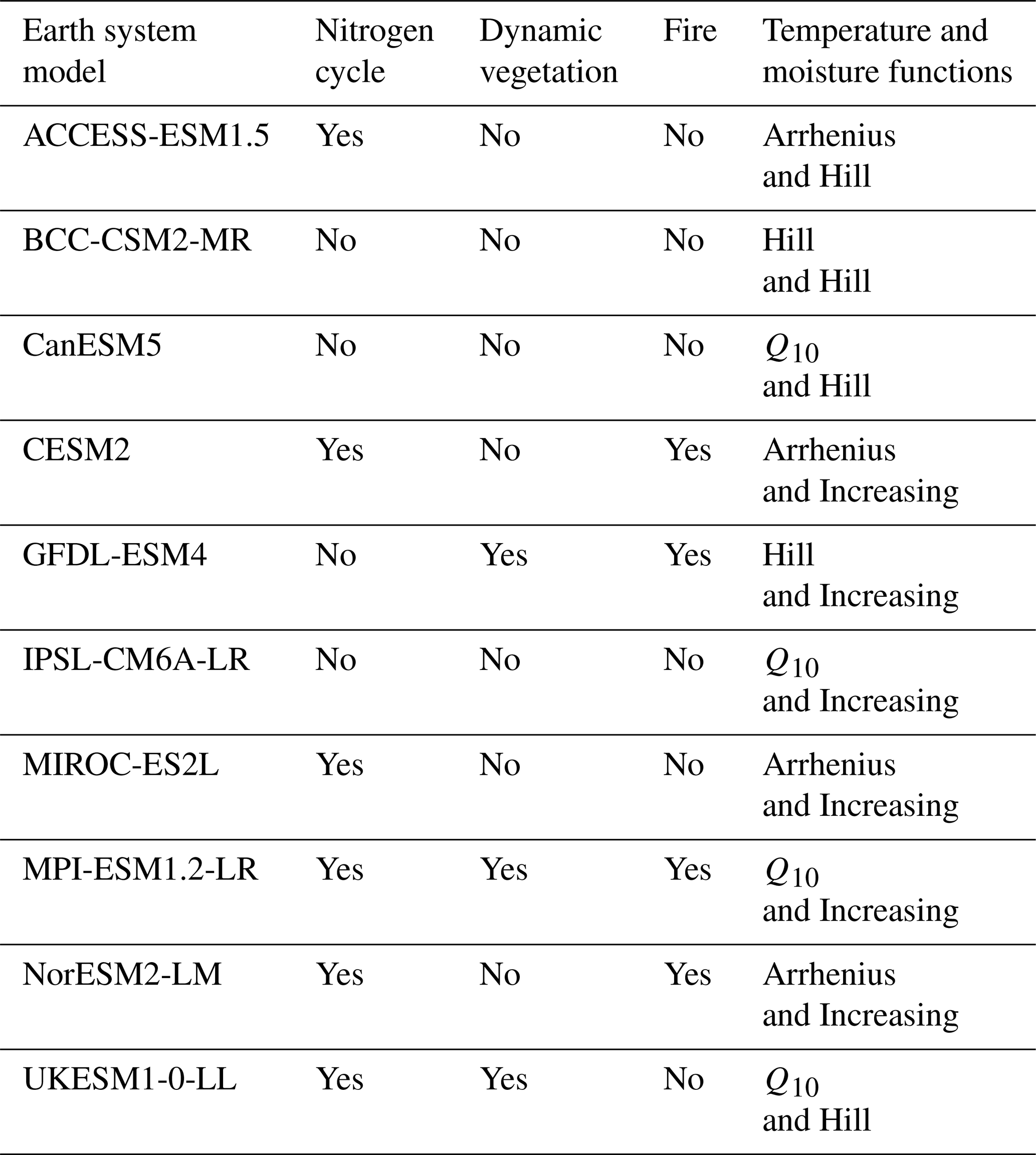
This study uses the full 1 % CO₂, BGC and RAD C4MIP experiments with 10 CMIP6 ESMs (Eyring et al., 2016): ACCESS-ESM1-5, BCC-CSM2-MR, CanESM5, CESM2, GFDL-ESM4, IPSL-CM6A-LR, MIROC-ES2L, MPI-ESM1-2-LR, NorESM2-LM and UKESM1-0-LL (see Table 1). For comparison, the soil carbon feedback parameters were calculated using six CMIP5 ESMs (Taylor et al., 2012): CanESM2, GFDL-ESM2M, IPSL-CM5A-LR, MPI-ESM-LR, NorESM1-ME and HadGEM2-ES (see Table A2). The ESMs included were chosen due to the availability of the data required at the time of analysis (CMIP6: https://esgf-node.llnl.gov/search/cmip6/, last access: 4 February 2024, CMIP5: https://esgf-node.llnl.gov/search/cmip5/, last access: 6 February 2024).

Table 1 The CMIP6 Earth system models included in this study and the relevant features of the associated land carbon cycle components: simulation of interactive nitrogen, the inclusion of dynamic vegetation, representation of fire and the soil decomposition functions used (Varney et al., 2022; Arora et al., 2020). Explanations of the temperature and moisture functions used within ESMs are given in Varney et al. (2022) and Todd-Brown et al. (2013).

2.2 Defining soil carbon feedbacks

2.2.1 Friedlingstein et al. (2006) βγ formulation

The standard formulation uses a linear approximation to estimate carbon cycle feedbacks in a changing climate (Friedlingstein et al., 2003, 2006). The change in land carbon storage (ΔC_L, PgC) is approximated linearly using feedback parameters which define separate sensitivities to changes in atmospheric CO₂ (ΔCO₂, ppm) and changes in global temperatures (ΔT, °C), defined as the land carbon-concentration (β_L, PgC ppm⁻¹) and carbon-climate (γ_L, PgC °C⁻¹) (Eq. 1).

$$\begin{array}{}\text{(1)}& \mathrm{\Delta }{C}_{\mathrm{L}}\approx {\mathit{\beta }}_{\mathrm{L}}\mathrm{\Delta }{\mathrm{CO}}_{\mathrm{2}}+{\mathit{\gamma }}_{\mathrm{L}}\mathrm{\Delta }T\end{array}$$

The Friedlingstein et al. (2006) methodology uses time-integrated fluxes, which represent the total change in the size of the land carbon pool (ΔC_L). This is presented for the full 1 % CO₂ simulation (Eq.  2), BGC simulation (Eq. 3) and RAD simulation (Eq. 4) below, where ΔC_L, $\mathrm{\Delta }{C}_{\mathrm{L}}^{\mathrm{BGC}}$ and $\mathrm{\Delta }{C}_{\mathrm{L}}^{\mathrm{RAD}}$ are the changes in global land carbon pools (PgC) and F_L, $F_{\mathrm{L}}^{\mathrm{BGC}}$ and $F_{\mathrm{L}}^{\mathrm{RAD}}$ are the net carbon fluxes to the land (PgC yr⁻¹) for each simulation.

$$\begin{array}{}\text{(2)}& {\displaystyle }\mathrm{\Delta }{C}_{\mathrm{L}}=\int F_{\mathrm{L}}\mathrm{d}t\approx {\mathit{\beta }}_{\mathrm{L}}\mathrm{\Delta }{\mathrm{CO}}_{\mathrm{2}}+{\mathit{\gamma }}_{\mathrm{L}}\mathrm{\Delta }T\text{(3)}& {\displaystyle }\mathrm{\Delta }{C}_{\mathrm{L}}^{\mathrm{BGC}}=\int F_{\mathrm{L}}^{\mathrm{BGC}}\mathrm{d}t\approx {\mathit{\beta }}_{\mathrm{L}}\mathrm{\Delta }{\mathrm{CO}}_{\mathrm{2}}+{\mathit{\gamma }}_{\mathrm{L}}\mathrm{\Delta }{T}^{\mathrm{BGC}}\approx {\mathit{\beta }}_{\mathrm{L}}\mathrm{\Delta }{\mathrm{CO}}_{\mathrm{2}}\text{(4)}& {\displaystyle }\mathrm{\Delta }{C}_{\mathrm{L}}^{\mathrm{RAD}}=\int F_{\mathrm{L}}^{\mathrm{RAD}}\mathrm{d}t\approx {\mathit{\gamma }}_{\mathrm{L}}\mathrm{\Delta }{T}^{\mathrm{RAD}}\end{array}$$

In these equations, ΔCO₂(t) (ppm) is consistent between all the scenarios. Within the RAD simulation, however (Eq. 4), the carbon cycle does not see an increased CO₂, so the ΔCO₂ is neglected and only found in the full 1 % CO₂ and BGC simulations (Eqs. 2 and 3, respectively). ΔT, ΔT^BGC and ΔT^RAD (°C) are the changes in global temperatures in the full 1 % CO₂, BGC and RAD simulations, respectively. In Eq. (3), ΔT^BGC is assumed to be negligible, following Friedlingstein et al. (2006). As the increased CO₂ within the BGC simulation does not affect the radiation code, there is no direct increase in atmospheric temperatures within the model. Arora et al. (2020) explain however that local changes in the carbon cycle arising from increases in CO₂ affect latent and sensible heat fluxes at the land surface, including changes to evaporative fluxes from stomatal closure over land and changes in vegetation structure and coverage if dynamic vegetation is included within the ESM (see Table 1). This study assumes that the global temperature changes in the BGC simulation are negligible in the context of the βγ formulation (Fig. A1).

2.2.2 Soil carbon-concentration and carbon-climate feedbacks

Global ΔC_L can be written as the sum of the changes in vegetation carbon (ΔC_v) and changes in soil carbon (ΔC_s). Following the βγ formulation, a similar breakdown of the land carbon-concentration and carbon-climate feedback parameters can be derived, where ${\mathit{\beta }}_{\mathrm{L}}={\mathit{\beta }}_{\mathrm{v}}+{\mathit{\beta }}_{\mathrm{s}}$ and ${\mathit{\gamma }}_{\mathrm{L}}={\mathit{\gamma }}_{\mathrm{v}}+{\mathit{\gamma }}_{\mathrm{s}}$ (Eq. 5).

$$\begin{array}{}\text{(5)}& {\displaystyle }\mathrm{\Delta }{C}_{\mathrm{L}}\approx \left({\mathit{\beta }}_{\mathrm{v}}+{\mathit{\beta }}_{\mathrm{s}}\right)\mathrm{\Delta }{\mathrm{CO}}_{\mathrm{2}}+\left({\mathit{\gamma }}_{\mathrm{v}}+{\mathit{\gamma }}_{\mathrm{s}}\right)\mathrm{\Delta }T\text{(6)}& {\displaystyle }\mathrm{\Delta }{C}_{\mathrm{v}}\approx {\mathit{\beta }}_{\mathrm{v}}\mathrm{\Delta }{\mathrm{CO}}_{\mathrm{2}}+{\mathit{\gamma }}_{\mathrm{v}}\mathrm{\Delta }T\text{(7)}& {\displaystyle }\mathrm{\Delta }{C}_{\mathrm{s}}\approx {\mathit{\beta }}_{\mathrm{s}}\mathrm{\Delta }{\mathrm{CO}}_{\mathrm{2}}+{\mathit{\gamma }}_{\mathrm{s}}\mathrm{\Delta }T\end{array}$$

Therefore, an equation for ΔC_s can be obtained, with soil-specific carbon-concentration (β_s) and carbon-climate (γ_s) feedback parameters, which represent the sensitivity of ΔC_s to CO₂ and T, respectively (Eq. 7).

2.3 Processes driving soil carbon change and the relation to the βγ formulation

To isolate the processes which make up each soil carbon feedback, we follow the framework presented in Varney et al. (2023). An equation for soil carbon (Eq. 8) is derived using the definition of soil carbon turnover time (${\mathit{\tau }}_{\mathrm{s}}=C_{\mathrm{s}}/R_{\mathrm{h}}$), which is defined as the ratio of soil carbon storage (C_s) to the carbon output flux from the soil (heterotrophic respiration, R_h; Varney et al., 2020). Future soil carbon can then be defined as initial soil carbon (C_s,0) plus a change in soil carbon (ΔC_s), as shown by Eq. 9, where the subscript 0 denotes the initial state (decadal time average at the start of C4MIP simulation). Equation (9) can be expanded to give Eq. (10), which can be simplified to give Eq. (11), as shown below.

$$\begin{array}{}\text{(8)}& {\displaystyle }{C}_{\mathrm{s}}=R_{\mathrm{h}}{\mathit{\tau }}_{\mathrm{s}}\text{(9)}& {\displaystyle }{C}_{\mathrm{s},\mathrm{0}}+\mathrm{\Delta }{C}_{\mathrm{s}}=\left(R_{\mathrm{h},\mathrm{0}}+\mathrm{\Delta }{R}_{\mathrm{h}}\right)\left({\mathit{\tau }}_{\mathrm{s},\mathrm{0}}+\mathrm{\Delta }{\mathit{\tau }}_{\mathrm{s}}\right)\text{(10)}& {\displaystyle }{C}_{\mathrm{s},\mathrm{0}}+\mathrm{\Delta }{C}_{\mathrm{s}}=R_{\mathrm{h},\mathrm{0}}{\mathit{\tau }}_{\mathrm{s},\mathrm{0}}+{\mathit{\tau }}_{\mathrm{s},\mathrm{0}}\mathrm{\Delta }{R}_{\mathrm{h}}+R_{\mathrm{h},\mathrm{0}}\mathrm{\Delta }{\mathit{\tau }}_{\mathrm{s}}+\mathrm{\Delta }{R}_{\mathrm{h}}\mathrm{\Delta }{\mathit{\tau }}_{\mathrm{s}}\text{(11)}& {\displaystyle }\mathrm{\Delta }{C}_{\mathrm{s}}={\mathit{\tau }}_{\mathrm{s},\mathrm{0}}\mathrm{\Delta }{R}_{\mathrm{h}}+R_{\mathrm{h},\mathrm{0}}\mathrm{\Delta }{\mathit{\tau }}_{\mathrm{s}}+\mathrm{\Delta }{R}_{\mathrm{h}}\mathrm{\Delta }{\mathit{\tau }}_{\mathrm{s}}\end{array}$$

To consider the above- and below-ground effects on soil carbon separately, the effects due to changes in vegetation productivity, represented by net primary productivity (NPP), and effects due to changes in soil carbon turnover time due to increased heterotrophic respiration (τ_s) are considered (Todd-Brown et al., 2014). However, due to the difference between the global fluxes NPP and R_h in a transient climate, an additional term is included which is defined as net ecosystem productivity ($\mathrm{NEP}=\mathrm{NPP}-R_{\mathrm{h}}$). Using the definition of NEP, this can be substituted into Eq. (11) to give Eq. (12) and expanded to give an equation for ΔC_s in terms of NPP, NEP and τ_s (Eq. 13, where the subscript 0 denotes the initial state).

$$\begin{array}{}\text{(12)}& {\displaystyle }\begin{array}{rl}\mathrm{\Delta }{C}_{\mathrm{s}}& ={\mathit{\tau }}_{\mathrm{s},\mathrm{0}}\mathrm{\Delta }(\mathrm{NPP}-\mathrm{NEP})+\left({\mathrm{NPP}}_{\mathrm{0}}-{\mathrm{NEP}}_{\mathrm{0}}\right)\mathrm{\Delta }{\mathit{\tau }}_{\mathrm{s}}\\ & +\mathrm{\Delta }(\mathrm{NPP}-\mathrm{NEP})\mathrm{\Delta }{\mathit{\tau }}_{\mathrm{s}}\end{array}\text{(13)}& {\displaystyle }\begin{array}{rl}\mathrm{\Delta }{C}_{\mathrm{s}}& ={\mathit{\tau }}_{\mathrm{s},\mathrm{0}}\mathrm{\Delta }\mathrm{NPP}+{\mathrm{NPP}}_{\mathrm{0}}\mathrm{\Delta }{\mathit{\tau }}_{\mathrm{s}}+\mathrm{\Delta }\mathrm{NPP}\mathrm{\Delta }{\mathit{\tau }}_{\mathrm{s}}\\ & -{\mathit{\tau }}_{\mathrm{s},\mathrm{0}}\mathrm{\Delta }\mathrm{NEP}-{\mathrm{NEP}}_{\mathrm{0}}\mathrm{\Delta }{\mathit{\tau }}_{\mathrm{s}}-\mathrm{\Delta }\mathrm{NEP}\mathrm{\Delta }{\mathit{\tau }}_{\mathrm{s}}\end{array}\end{array}$$

The individual terms in Eq. (13) are the change in soil carbon due to NPP changes ($\mathrm{\Delta }{C}_{\mathrm{s},\mathrm{NPP}}\approx {\mathit{\tau }}_{\mathrm{s},\mathrm{0}}\mathrm{\Delta }\mathrm{NPP}$), the change in soil carbon due to the NEP transient term ($\mathrm{\Delta }{C}_{\mathrm{s},\mathrm{NEP}}\approx -{\mathit{\tau }}_{\mathrm{s},\mathrm{0}}\mathrm{\Delta }\mathrm{NEP}$), the change in soil carbon due to τ_s changes ($\mathrm{\Delta }{C}_{\mathrm{s},\mathit{\tau }}\approx {\mathrm{NPP}}_{\mathrm{0}}\mathrm{\Delta }{\mathit{\tau }}_{\mathrm{s}}$) and the transient effect on τ_s ($\mathrm{\Delta }{C}_{\mathrm{s},{\mathit{\tau }}_{\mathrm{NEP}}}\approx -{\mathrm{NEP}}_{\mathrm{0}}\mathrm{\Delta }{\mathit{\tau }}_{\mathrm{s}}$). The two additional terms are the non-linear term between NPP and τ_s (ΔNPPΔτ_s) and the non-linear term between NEP and τ_s (ΔNEPΔτ_s).

The NEP term is used to represent the transient state of the system where NPP ≠ R_h. However, it is noted that, if the initial state is in equilibrium, then the initial NEP (NEP₀) will be approximately equal to zero. This would mean the $\mathrm{\Delta }{C}_{\mathrm{s},{\mathit{\tau }}_{\mathrm{NEP}}}$ term (representing the difference in τ_s from using NPP or R_h in the definition) will be negligible. Despite initialising at the start of the C4MIP simulations (decadal time average at the start of C4MIP simulation), this term is included within the analysis for completeness to ensure exact values of ΔC_s.

Following on from this Varney et al. (2023) framework, the equation for ΔC_s (Eq. 13) can also be defined for the change in soil carbon in both the BGC simulations ($\mathrm{\Delta }{C}_{\mathrm{s}}^{\mathrm{BGC}}$, Eq. 14) and RAD simulations ($\mathrm{\Delta }{C}_{\mathrm{s}}^{\mathrm{RAD}}$, Eq. 15), where the superscripts denote the BGC and RAD simulations, respectively.

$$\begin{array}{}\text{(14)}& {\displaystyle }\begin{array}{rl}\mathrm{\Delta }{C}_{\mathrm{s}}^{\mathrm{BGC}}& ={\mathit{\tau }}_{\mathrm{s},\mathrm{0}}^{\mathrm{BGC}}\mathrm{\Delta }{\mathrm{NPP}}^{\mathrm{BGC}}\\ & +{\mathrm{NPP}}_{\mathrm{0}}^{\mathrm{BGC}}\mathrm{\Delta }{\mathit{\tau }}_{\mathrm{s}}^{\mathrm{BGC}}+\mathrm{\Delta }{\mathrm{NPP}}^{\mathrm{BGC}}\mathrm{\Delta }{\mathit{\tau }}_{\mathrm{s}}^{\mathrm{BGC}}\\ & -{\mathit{\tau }}_{\mathrm{s},\mathrm{0}}^{\mathrm{BGC}}\mathrm{\Delta }{\mathrm{NEP}}^{\mathrm{BGC}}-{\mathrm{NEP}}_{\mathrm{0}}^{\mathrm{BGC}}\mathrm{\Delta }{\mathit{\tau }}_{\mathrm{s}}^{\mathrm{BGC}}\\ & -\mathrm{\Delta }{\mathrm{NEP}}^{\mathrm{BGC}}\mathrm{\Delta }{\mathit{\tau }}_{\mathrm{s}}^{\mathrm{BGC}}\end{array}\text{(15)}& {\displaystyle }\begin{array}{rl}\mathrm{\Delta }{C}_{\mathrm{s}}^{\mathrm{RAD}}& ={\mathit{\tau }}_{\mathrm{s},\mathrm{0}}^{\mathrm{RAD}}\mathrm{\Delta }{\mathrm{NPP}}^{\mathrm{RAD}}\\ & +{\mathrm{NPP}}_{\mathrm{0}}^{\mathrm{RAD}}\mathrm{\Delta }{\mathit{\tau }}_{\mathrm{s}}^{\mathrm{RAD}}+\mathrm{\Delta }{\mathrm{NPP}}^{\mathrm{RAD}}\mathrm{\Delta }{\mathit{\tau }}_{\mathrm{s}}^{\mathrm{RAD}}\\ & -{\mathit{\tau }}_{\mathrm{s},\mathrm{0}}^{\mathrm{RAD}}\mathrm{\Delta }{\mathrm{NEP}}^{\mathrm{RAD}}-{\mathrm{NEP}}_{\mathrm{0}}^{\mathrm{RAD}}\mathrm{\Delta }{\mathit{\tau }}_{\mathrm{s}}^{\mathrm{RAD}}\\ & -\mathrm{\Delta }{\mathrm{NEP}}^{\mathrm{RAD}}\mathrm{\Delta }{\mathit{\tau }}_{\mathrm{s}}^{\mathrm{RAD}}\end{array}\end{array}$$

These equations can be used to investigate the sensitivity of these isolated processes to changes in atmospheric CO₂ and global temperature (T), as shown by Eqs. (16) and (17). This is done by the explicit differentiation of Eqs. (14) and (15) with respect to CO₂ and T, respectively.

$$\begin{array}{}\text{(16)}& {\displaystyle }\mathrm{\Delta }{C}_{\mathrm{s}}^{\mathrm{BGC}}={\displaystyle \frac{\partial }{\partial {\mathrm{CO}}_{\mathrm{2}}}}\left[\mathrm{\Delta }{C}_{\mathrm{s}}^{\mathrm{BGC}}\right]\mathrm{\Delta }{\mathrm{CO}}_{\mathrm{2}}\text{(17)}& {\displaystyle }\mathrm{\Delta }{C}_{\mathrm{s}}^{\mathrm{RAD}}={\displaystyle \frac{\partial }{\partial T}}\left[\mathrm{\Delta }{C}_{\mathrm{s}}^{\mathrm{RAD}}\right]\mathrm{\Delta }T\end{array}$$

Equations (16) and (17) can be used to relate these CO₂ and T sensitivities to the βγ formulation, where β is used to represent the sensitivity to CO₂ and γ is used to represent the sensitivity to T. Equation (7), which defines ΔC_s in terms of the soil carbon-concentration (β_s) and carbon-climate (γ_s) feedback parameters, can be rewritten in terms of partial derivatives, as shown by Eq. (18).

$$\begin{array}{}\text{(18)}& \begin{array}{rl}\mathrm{\Delta }{C}_{\mathrm{s}}=& {\displaystyle \frac{\partial C_{\mathrm{s}}}{\partial {\mathrm{CO}}_{\mathrm{2}}}}\mathrm{\Delta }{\mathrm{CO}}_{\mathrm{2}}+{\displaystyle \frac{\partial C_{\mathrm{s}}}{\partial T}}\mathrm{\Delta }T\\ & \mathrm{where},{\mathit{\beta }}_{\mathrm{s}}=\partial C_{\mathrm{s}}/\partial {\mathrm{CO}}_{\mathrm{2}}\\ & \mathrm{and}{\mathit{\gamma }}_{\mathrm{s}}=\partial C_{\mathrm{s}}/\partial T\end{array}\end{array}$$

Then, Eqs. (16) and (17) can be used together with Eq. (18) to combine the βγ formulation with the Varney et al. (2023) framework. In this case, therefore, β_s and γ_s can be defined as the contributions to ΔC_s based on the individual sensitivities of the soil carbon controls to CO₂ and T (by substituting Eqs. (14) and (15) into Eqs. (16) and (17), respectively), as shown by Eqs. (20) and (21).

$$\begin{array}{}\text{(19)}& \mathrm{\Delta }{C}_{\mathrm{s}}={\displaystyle \frac{\partial }{\partial {\mathrm{CO}}_{\mathrm{2}}}}\left[\mathrm{\Delta }{C}_{\mathrm{s}}^{\mathrm{BGC}}\right]\mathrm{\Delta }{\mathrm{CO}}_{\mathrm{2}}+{\displaystyle \frac{\partial }{\partial T}}\left[\mathrm{\Delta }{C}_{\mathrm{s}}^{\mathrm{RAD}}\right]\mathrm{\Delta }T,\end{array}$$

where

$$\begin{array}{}\text{(20)}& {\displaystyle }\begin{array}{rl}{\mathit{\beta }}_{\mathrm{s}}& ={\mathit{\tau }}_{\mathrm{s},\mathrm{0}}^{\mathrm{BGC}}{\displaystyle \frac{\partial {\mathrm{NPP}}^{\mathrm{BGC}}}{\partial {\mathrm{CO}}_{\mathrm{2}}}}\\ & +{\mathrm{NPP}}_{\mathrm{0}}^{\mathrm{BGC}}{\displaystyle \frac{\partial {\mathit{\tau }}_{\mathrm{s}}^{\mathrm{BGC}}}{\partial {\mathrm{CO}}_{\mathrm{2}}}}+{\displaystyle \frac{\partial \mathrm{\Delta }{\mathrm{NPP}}^{\mathrm{BGC}}\mathrm{\Delta }{\mathit{\tau }}_{\mathrm{s}}^{\mathrm{BGC}}}{\partial {\mathrm{CO}}_{\mathrm{2}}}}\\ & -{\mathit{\tau }}_{\mathrm{s},\mathrm{0}}^{\mathrm{BGC}}{\displaystyle \frac{\partial {\mathrm{NEP}}^{\mathrm{BGC}}}{\partial {\mathrm{CO}}_{\mathrm{2}}}}-{\mathrm{NEP}}_{\mathrm{0}}^{\mathrm{BGC}}{\displaystyle \frac{\partial {\mathit{\tau }}_{\mathrm{s}}^{\mathrm{BGC}}}{\partial {\mathrm{CO}}_{\mathrm{2}}}}\\ & -{\displaystyle \frac{\partial \mathrm{\Delta }{\mathrm{NEP}}^{\mathrm{BGC}}\mathrm{\Delta }{\mathit{\tau }}_{\mathrm{s}}^{\mathrm{BGC}}}{\partial {\mathrm{CO}}_{\mathrm{2}}}},\end{array}\text{(21)}& {\displaystyle }\begin{array}{rl}{\mathit{\gamma }}_{\mathrm{s}}& ={\mathit{\tau }}_{\mathrm{s},\mathrm{0}}^{\mathrm{RAD}}{\displaystyle \frac{\partial {\mathrm{NPP}}^{\mathrm{RAD}}}{\partial T}}+{\mathrm{NPP}}_{\mathrm{0}}^{\mathrm{RAD}}{\displaystyle \frac{\partial {\mathit{\tau }}_{\mathrm{s}}^{\mathrm{RAD}}}{\partial T}}\\ & +{\displaystyle \frac{\partial \mathrm{\Delta }{\mathrm{NPP}}^{\mathrm{RAD}}\mathrm{\Delta }{\mathit{\tau }}_{\mathrm{s}}^{\mathrm{RAD}}}{\partial T}}\\ & -{\mathit{\tau }}_{\mathrm{s},\mathrm{0}}^{\mathrm{RAD}}{\displaystyle \frac{\partial {\mathrm{NEP}}^{\mathrm{RAD}}}{\partial T}}-{\mathrm{NEP}}_{\mathrm{0}}^{\mathrm{RAD}}{\displaystyle \frac{\partial {\mathit{\tau }}_{\mathrm{s}}^{\mathrm{RAD}}}{\partial T}}\\ & -{\displaystyle \frac{\partial \mathrm{\Delta }{\mathrm{NEP}}^{\mathrm{RAD}}\mathrm{\Delta }{\mathit{\tau }}_{\mathrm{s}}^{\mathrm{RAD}}}{\partial T}}.\end{array}\end{array}$$

Equations (20) and (21) can be rewritten by defining the β_s and γ_s contribution terms, where each component of the equations makes up the total β_s and γ_s sensitivities, as shown below for β_s (Eq. 22) and γ_s (Eq. 23):

$$\begin{array}{}\text{(22)}& {\displaystyle }{\mathit{\beta }}_{\mathrm{s}}={\mathit{\beta }}_{\mathrm{NPP}}+{\mathit{\beta }}_{\mathit{\tau }}+{\mathit{\beta }}_{\mathrm{\Delta }\mathrm{NPP}\mathrm{\Delta }\mathit{\tau }}-{\mathit{\beta }}_{\mathrm{NEP}}-{\mathit{\beta }}_{{\mathrm{NEP}}_{\mathit{\tau }}}-{\mathit{\beta }}_{\mathrm{\Delta }\mathrm{NEP}\mathrm{\Delta }\mathit{\tau }},\text{(23)}& {\displaystyle }{\mathit{\gamma }}_{\mathrm{s}}={\mathit{\gamma }}_{\mathrm{NPP}}+{\mathit{\gamma }}_{\mathit{\tau }}+{\mathit{\gamma }}_{\mathrm{\Delta }\mathrm{NPP}\mathrm{\Delta }\mathit{\tau }}-{\mathit{\gamma }}_{\mathrm{NEP}}-{\mathit{\gamma }}_{{\mathrm{NEP}}_{\mathit{\tau }}}-{\mathit{\gamma }}_{\mathrm{\Delta }\mathrm{NEP}\mathrm{\Delta }\mathit{\tau }},\end{array}$$

where β_NPP and γ_NPP are the βγ contributions due to ΔNPP, β_τ and γ_τ are the βγ contributions due to Δτ_s, β_NEP and γ_NEP are the βγ contributions due to the transient NEP term, including ${\mathit{\beta }}_{{\mathrm{NEP}}_{\mathit{\tau }}}$ and ${\mathit{\gamma }}_{{\mathrm{NEP}}_{\mathit{\tau }}}$ representing the βγ contributions due to the transient NEP term on Δτ_s, and then β_ΔNPPΔτ, β_ΔNEPΔτ, γ_ΔNPPΔτ and γ_ΔNEPΔτ are the non-linear effects on βγ.

2.4 Calculation of feedback parameters

2.4.1 Defining climate variables

For each of the CMIP6 ESMs, the CMIP output variables cSoil, cLitter and cVeg are considered in the land carbon storage analysis. Soil carbon (C_s) is defined as the sum of carbon stored in soils and the carbon stored in the litter (CMIP variable cSoil + CMIP variable cLitter), allowing for a more consistent comparison between the models despite differences in how soil carbon and litter carbon are simulated (Varney et al., 2022; Todd-Brown et al., 2013). For models that do not report a separate litter carbon pool (CMIP variable cLitter), soil carbon is taken to be simply the CMIP variable cSoil (UKESM1-0-LL). Land carbon (C_L) is defined as the sum of carbon stored in soil + litter (C_s) plus the carbon stored in vegetation (C_v, CMIP variable cVeg). Global total values for C_s and C_L (PgC) are calculated using an area-weighted sum (using the model land surface fraction, CMIP variable sftlf).

In the breakdown analysis of the βγ feedbacks, NPP (CMIP variable npp) is defined as the net carbon assimilated by plants via photosynthesis minus loss due to plant respiration and is used to represent the net carbon input flux to the system. Heterotrophic respiration (R_h, CMIP variable rh) is defined as the microbial respiration within global soils and is used to define an effective global soil carbon turnover time (τ_s). τ_s (years) is defined as the ratio of mean soil carbon to annual mean heterotrophic respiration, given as ${\mathit{\tau }}_{\mathrm{s}}=C_{\mathrm{s}}/R_{\mathrm{h}}$ (where the mean represents an area-weighted global average). Carbon fluxes (NPP and R_h) in the calculation of feedback contributions are considered area-weighted global totals (PgC yr⁻¹, using the model land surface fraction, CMIP variable sftlf).

Increases in global temperatures (ΔT) are considered using CMIP variable tas, which is defined as the change in near-surface air temperature (°C). To calculate changes in atmospheric CO₂ (ΔCO₂) in the C4MIP 1 % CO₂ simulations, initial pre-industrial CO₂ concentrations are assumed to be 285 ppm and then cumulatively increased by 1 % each year for 70 years (approximately 2 × CO₂) or 140 years (approximately 4 × CO₂).

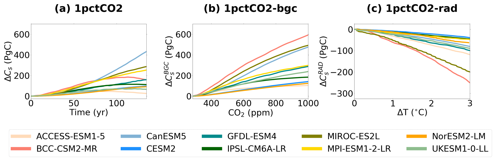
Figure 1 Time series of projected changes in soil carbon (ΔC_s) in CMIP6 ESMs for the (a) idealised 1 % CO₂, (b) biogeochemically coupled 1 % CO₂ (BGC) and (c) radiatively coupled 1 % CO₂ (RAD) simulations. This figure has been adapted from Fig. A2 in Varney et al. (2023).

2.4.2 Carbon-concentration feedback parameter (β)

To calculate the soil carbon-concentration feedback parameter (β_s), the BGC run was used. For each ESM, the change in soil carbon in the BGC run ($\mathrm{\Delta }{C}_{\mathrm{s}}^{\mathrm{BGC}}$, PgC) was divided by the change in CO₂ concentration (ppm) up to that point in time (expressed in units of carbon uptake or release per unit change in CO₂, PgC ppm⁻¹). For this study, β_s was calculated at the time of 2 × CO₂ and 4 × CO₂. To calculate the land carbon-concentration feedback parameter (β_L), the same method was used but replacing $C_{\mathrm{s}}^{\mathrm{BGC}}$ with $C_{\mathrm{L}}^{\mathrm{BGC}}$.

2.4.3 Carbon-climate feedback parameter (γ)

To calculate the soil carbon-climate feedback parameter (γ_s), the RAD run was used. For each ESM, the change in soil carbon in the RAD run ($\mathrm{\Delta }{C}_{\mathrm{s}}^{\mathrm{RAD}}$, PgC) was divided by the change in temperature T (°C) up to that point in time (expressed in units of carbon uptake or release per unit change in temperature, PgC °C⁻¹). For this study, γ_s was calculated at 2 × CO₂ and 4 × CO₂. To calculate the land carbon-climate feedback parameter (γ_L), the same method was used but replacing $C_{\mathrm{s}}^{\mathrm{RAD}}$ with $C_{\mathrm{L}}^{\mathrm{RAD}}$.

2.4.4 Feedback parameter contributions

To calculate the isolated contributions which make up β and γ, as shown in Eqs. (22) and (23), the BGC and RAD simulations are again used for each CMIP6 ESM. To calculate gradients with respect to CO₂ and T, the methodology presented above is used but with the relevant component against CO₂ or T, such as NPP or τ_s. The β_s contributions are expressed in units of carbon uptake or release per unit change in CO₂ (PgC ppm⁻¹) and the γ_s contributions are expressed in units of carbon uptake or release per unit change in temperature (PgC °C⁻¹), using the definitions presented in Eqs. (22) and (23).

3 Results

3.1 Projections of soil carbon change

Projections of soil carbon change in CMIP6 ESMs for the full 1 % CO₂ (ΔC_s), BGC ($\mathrm{\Delta }{C}_{\mathrm{s}}^{\mathrm{BGC}}$) and RAD ($\mathrm{\Delta }{C}_{\mathrm{s}}^{\mathrm{RAD}}$) simulations are presented in Fig. 1. Soil carbon is projected to increase in the full 1 % CO₂ simulation amongst CMIP6 ESMs (ensemble mean 88.2 ± 40.4 PgC at 2 × CO₂ and 177 ± 141 PgC at 4 × CO₂). However, the magnitude of the increase varies amongst the ESMs, with a range of 38 PgC (NorESM2-LM) to 145 PgC (BCC-CSM2-MR) at 2 × CO₂ and a range of 15 PgC (ACCESS-ESM1-5) to 502 PgC (CanESM5) at 4 × CO₂. Six of the ESMs (CanESM5, CESM2, GFDL-ESM4, MIROC-ES2L, MPI-ESM1-2-LR, NorESM2-LM) see an increased ΔC_s value with increasing climate forcing. However, the remaining four ESMs (ACCESS-ESM1-5, BCC-CSM2-MR, IPSL-CM6A-LR, UKESM1-0-LL) see a saturation in the rate of increase or even a turning point where carbon starts to decrease again, from 70 years (≈ 2 × CO₂) in the simulation (Fig. 1a).

The projected increase in soil carbon can be approximated by the increases projected in the BGC run ($\mathrm{\Delta }{C}_{\mathrm{s}}^{\mathrm{BGC}}$; ensemble mean 132 ± 66.5 PgC at 2 × CO₂ and 348 ± 203 PgC at 4 × CO₂, Fig. 1b) and the decreases projected in the RAD run ($\mathrm{\Delta }{C}_{\mathrm{s}}^{\mathrm{RAD}}$; ensemble mean −45.5 ± 22.9 PgC at 2 × CO₂ and −170 ± 94.7 PgC at 4 × CO₂, Fig. 1c). The responses due to increases in atmospheric CO₂ (BGC simulation) are found to dominate the overall response (full 1 % CO₂ simulation) in the majority of the models, where greater magnitudes of change are seen compared with the RAD simulation (exception ACCESS-ESM1-5). The BGC simulation also sees a greater spread in projected ΔC_s, with ranges of 218 PgC at 2 × CO₂ and 603 PgC at 4 × CO₂ ($\mathrm{\Delta }{C}_{\mathrm{s}}^{\mathrm{BGC}}$) compared with ranges of 68 PgC at 2 × CO₂ and 312 PgC at 4 × CO₂ in the RAD simulation ($\mathrm{\Delta }{C}_{\mathrm{s}}^{\mathrm{RAD}}$).

Figure 2 shows patterns of soil carbon changes at 4 × CO₂ for the full 1 % CO₂ (ΔC_s), BGC ($\mathrm{\Delta }{C}_{\mathrm{s}}^{\mathrm{BGC}}$) and RAD ($\mathrm{\Delta }{C}_{\mathrm{s}}^{\mathrm{RAD}}$). In the BGC simulation, increases in $\mathrm{\Delta }{C}_{\mathrm{s}}^{\mathrm{BGC}}$ are seen across the majority of regions within CMIP6 ESMs, though exceptions are found at the northern latitudes for two ESMs (CanESM5 and NorESM2-LM). Across the ensemble, the projected increases in $\mathrm{\Delta }{C}_{\mathrm{s}}^{\mathrm{BGC}}$ have spatially varying magnitudes, where generally the greatest increases are seen in the tropical regions. Conversely, the RAD simulation generally sees reductions in $\mathrm{\Delta }{C}_{\mathrm{s}}^{\mathrm{RAD}}$ globally, with the greatest reductions seen in the tropical regions. However, disagreement is seen at the northern latitudes, where four models (ACCESS-ESM1-5, CanESM5, MIROC-ES2L, UKESM1-0-LL) see an increased $\mathrm{\Delta }{C}_{\mathrm{s}}^{\mathrm{RAD}}$ and three models (BCC-CSM2-MR, CESM2, NorESM2-LM) see a decreased $\mathrm{\Delta }{C}_{\mathrm{s}}^{\mathrm{RAD}}$. The overall ΔC_s values seen in the full 1 % CO₂ simulation are again found to be mostly dominated by the BGC simulation (Fig. 2), though exceptions are seen where the RAD simulation is shown to dominate the response for certain regions. Specifically, the reduced ΔC_s within the RAD simulation dominates the net response at the northern latitudes of three ESMs (BCC-CSM2-MR, CESM2 and NorESM2-LM, the only models where decreases were seen) as well as in the tropical regions of three different ESMs (ACCESS-ESM1-5, GFDL-ESM4 and UKESM1-0-LL).

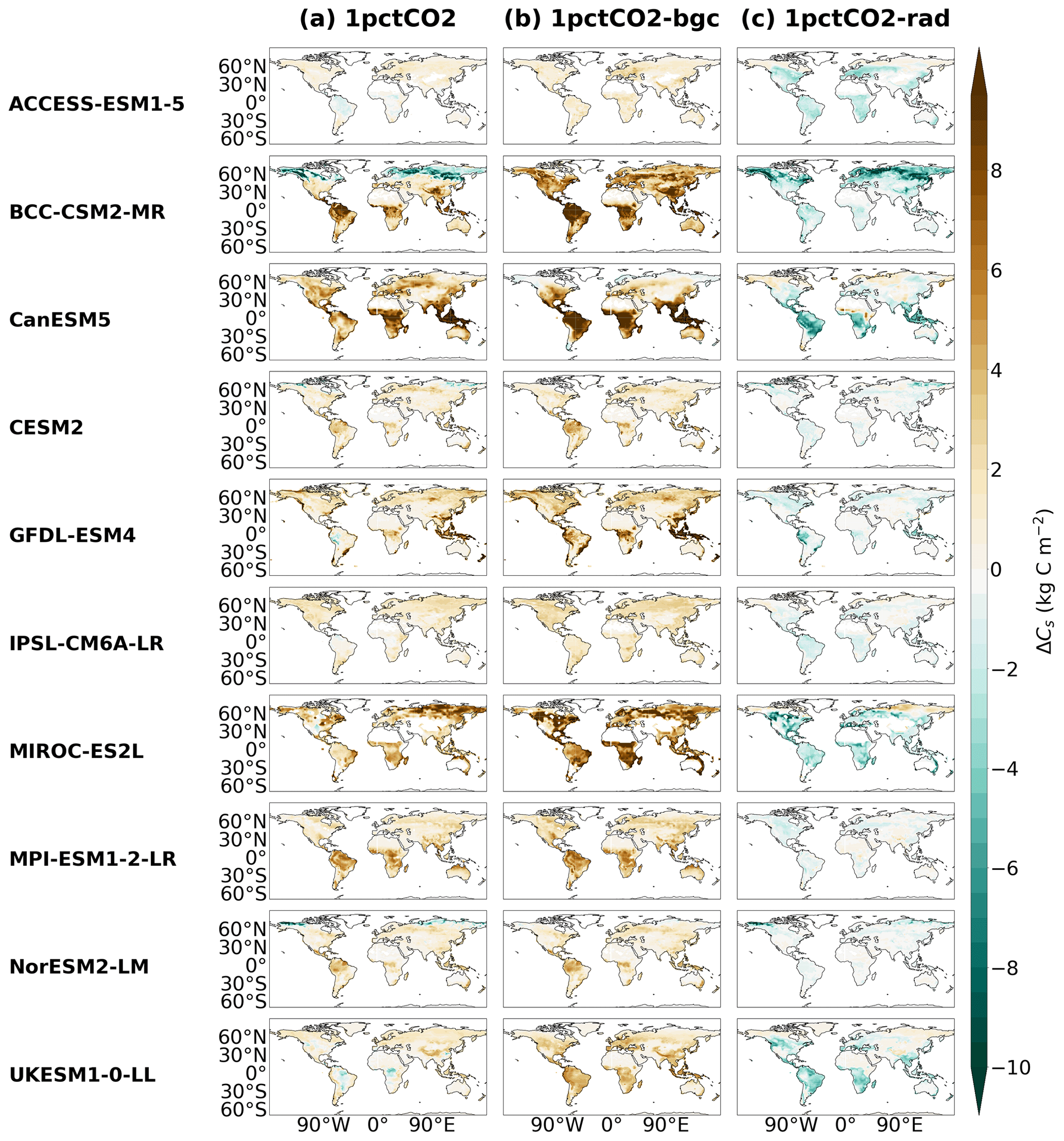
Figure 2 Maps showing the changes in soil carbon (ΔC_s) at 4 × CO₂ in CMIP6 ESMs, for the (a) idealised simulation 1 % CO₂ (left column), (b) biogeochemically coupled 1 % CO₂ (BGC, middle column) and (c) radiatively coupled 1 % CO₂ (RAD, right column).

3.2 Soil carbon-concentration and carbon-climate feedback parameters

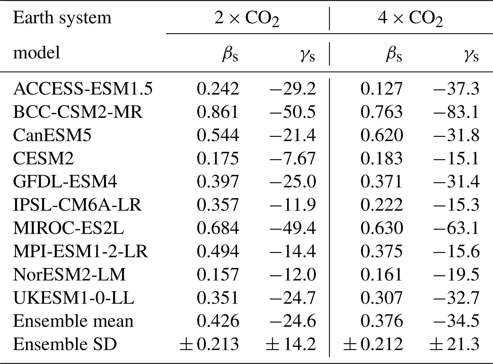
The calculated β_s and γ_s values for CMIP6 ESMs are presented in Table 2. Values for β_s are found to be positive amongst the CMIP6 ESMs, which is consistent with increased C_s with increasing CO₂, and values for γ_s are found to be negative, which is consistent with decreased C_s with increasing temperature (Fig. 3). The magnitudes of the feedback parameters (β_s and γ_s) are found to vary amongst the CMIP6 ensemble, suggesting uncertainty in the magnitude of the soil carbon response to climate change. Generally, models with higher sensitivities to CO₂ (β_s) also have higher sensitivities to temperature (γ_s), where r² values of 0.64 (2 × CO₂) and 0.60 (4 × CO₂) are found between the β_s and γ_s values (Table 2). The ranges in projected β_s parameters are found to be relatively consistent between 2 × CO₂ and 4 × CO₂ (where a small decrease is seen), with a range of 0.704 PgC ppm⁻¹ and a range of 0.636 PgC ppm⁻¹, respectively. Conversely, the ranges of calculated γ_s parameters are found to be less consistent between 2 × CO₂ and 4 × CO₂ (increasing range with increased global warming), with ranges of 42.7 and 68.0 PgC °C⁻¹, respectively (Table 2).

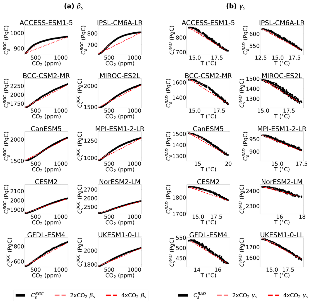
Figure 3 Time series plots used to calculate the soil feedback parameters. (a) Soil carbon in the BGC simulation ($C_{\mathrm{s}}^{\mathrm{BGC}}$, PgC) vs. CO₂ (ppm) for the carbon-concentration feedback parameters (β_s, PgC ppm⁻¹) and (b) soil carbon in the RAD simulation ($C_{\mathrm{s}}^{\mathrm{RAD}}$, PgC) vs. temperature (T, °C) for the soil carbon-climate feedback parameters (γ_s, PgC °C⁻¹), for each CMIP6 ESM. The lines show the gradients at 2 × CO₂ (lighter line) and 4 × CO₂ (darker line), respectively.

The linearity of future soil carbon changes can be investigated by comparing the 2 × CO₂ and 4 × CO₂ lines for β_s and γ_s in Fig. 3. A future linear response is shown to be a good approximation. However, the figure suggests a slight non-linearity in the soil carbon response to both CO₂ ($\mathrm{\Delta }{C}_{\mathrm{s}}^{\mathrm{BGC}}$) and temperature ($\mathrm{\Delta }{C}_{\mathrm{s}}^{\mathrm{RAD}}$) in the majority of ESMs. The BGC simulation generally sees greater consistency between 2 × CO₂ and 4 × CO₂ β_s values, for example in the CESM2 and NorESM2-LM models. However, the majority of ESMs (ACCESS-ESM1-5, BCC-CSM2-MR, GFDL-ESM4, IPSL-CM6A-LR, MIROC-ES2L, MPI-ESM1-2-LR and UKESM1-0-LL) see a reduction in β_s and a saturation in the sensitivity with greater CO₂ levels (Fig. 3a). In the RAD simulation, generally inconsistencies are seen between 2 × CO₂ and 4 × CO₂ (exception MPI-ESM1-2-LR), and an increased sensitivity of $C_{\mathrm{s}}^{\mathrm{RAD}}$ to temperature (T) with increased climate forcing is suggested by the majority of CMIP6 ESMs (Fig. 3b). As an example, in CESM2, where one of the lowest sensitivities to T at 2 × CO₂ is seen, the ESM sees an approximate 50 % increase in γ_s by 4 × CO₂ (Table 2).

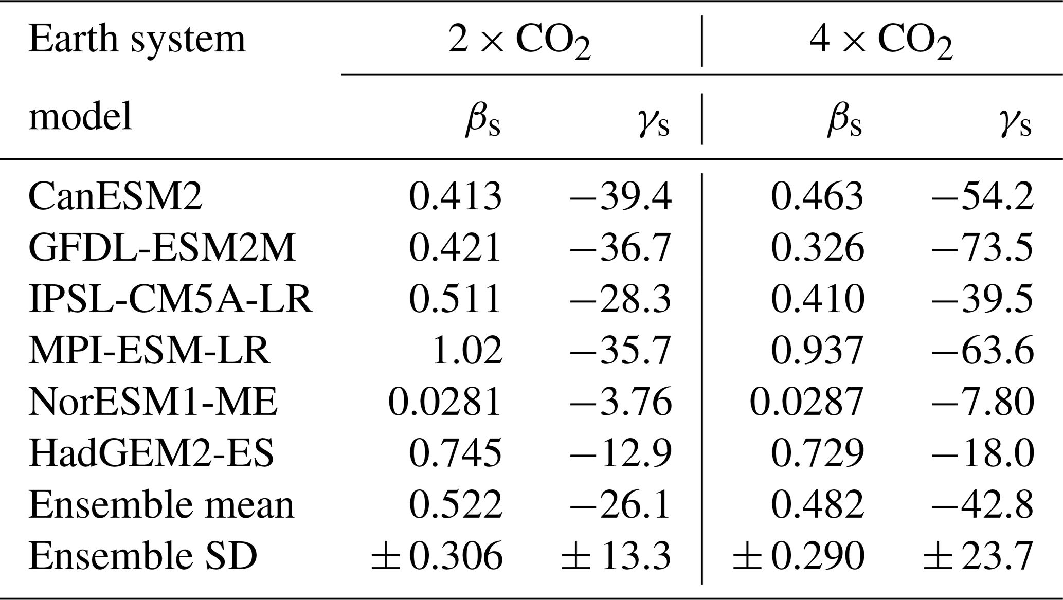
The β_s and γ_s values were also calculated for CMIP5 ESMs (Table A3), which can be compared with a subset of generationally related CMIP6 ESMs considered in this study (Fig. A3). The CMIP6 ensemble means for both β_s and γ_s parameters are found to be lower compared with the CMIP5 ensemble means (Tables 2 and A3). The relationship of β_s and γ_s values between CMIP5 and CMIP6, however, is not found to be consistent amongst the ensembles. For β_s, reductions are seen in four ESMs (GFDL-ESM2M vs. GFDL-ESM4, IPSL-CM5A-LR vs. IPSL-CM6A-LR, MPI-ESM-LR vs. MPI-ESM1-2-LR and HadGEM2-ES vs. UKESM1-0-LL) compared with increases in the remaining two (CanESM2 vs. CanESM5 and NorESM1-ME vs. NorESM2-LM). For γ_s, a greater value (closer to 0) is seen in four ESMs (CanESM2 vs. CanESM5, GFDL-ESM2M vs. GFDL-ESM4, IPSL-CM5A-LR vs. IPSL-CM6A-LR and MPI-ESM-LR vs. MPI-ESM1-2-LR) compared with a lower value (greater negative) seen in the remaining two ESMs (NorESM1-ME vs. NorESM2-LM and HadGEM2-ES vs. UKESM1-0-LL).

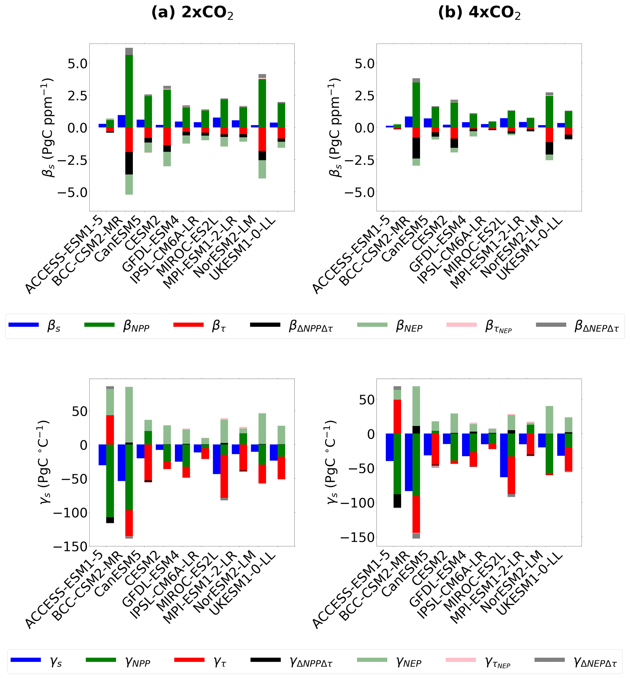
Figure 4 Investigating the contribution of individual soil carbon drivers to the soil carbon-concentration (β_s, top row) and carbon-climate (γ_s, bottom row) feedback parameters, for each CMIP6 ESM, for (a) 2 × CO₂ and (b) 4 × CO₂. The figure shows soil carbon feedback parameter contributions from NPP (β_NPP and γ_NPP), τ_s (β_τ and γ_τ), the non-linearity in NPP and τ_s (β_ΔNPPΔτ and γ_ΔNPPΔτ) and the effect from the non-equilibrium term NEP (β_NEP, ${\mathit{\beta }}_{{\mathit{\tau }}_{\mathrm{NEP}}}$, β_ΔNEPΔτ and γ_NEP, ${\mathit{\gamma }}_{{\mathit{\tau }}_{\mathrm{NEP}}}$, γ_ΔNEPΔτ).

3.3 Breakdown of the feedback parameters into soil carbon drivers

In this section, β_s and γ_s are broken down into the individual sensitivities of drivers of soil carbon change which make up the net response. As shown in Fig. 4, the total soil carbon sensitivities (β_s and γ_s, blue bars) can be considered as the sum of the sensitivity due to ΔNPP (β_NPP and γ_NPP, green bars), the sensitivity due to Δτ_s (β_τ and γ_τ, red bars) and additional terms due to the transient land carbon sink, such as NEP (β_NEP and γ_NEP, light green bars) and the NEP effect on τ_s (${\mathit{\beta }}_{{\mathit{\tau }}_{\mathrm{NEP}}}$ and ${\mathit{\gamma }}_{{\mathit{\tau }}_{\mathrm{NEP}}}$, pink bars). Additionally, there are non-negligible contributions due to non-linear sensitivities between NPP and τ_s (β_ΔNPPΔτ and γ_ΔNPPΔτ, black bars) and a small contribution from non-linear sensitivities between NEP and τ_s (β_ΔNEPΔτ and γ_ΔNEPΔτ, grey bars).

Table 2 The soil carbon-concentration (β_s, PgC ppm⁻¹) and carbon-climate (γ_s, PgC °C⁻¹) feedback parameters for 2 × CO₂ and 4 × CO₂ for the CMIP6 ESMs.

Investigating the sensitivity of soil carbon to ΔNPP, β_NPP is found to be positive amongst CMIP6 ESMs (Fig. 4). At 2 × CO₂, β_NPP ranges from 0.567 PgC ppm⁻¹ (ACCESS-ESM1-5) to 5.62 PgC ppm⁻¹ (BCC-CSM2-MR), with an ensemble mean of 2.37 ± 1.37 PgC ppm⁻¹. There is some evidence of a saturation of global NPP at higher CO₂, with the sensitivity of NPP to CO₂ (β_NPP) decreasing at 4 × CO₂ to an ensemble mean of 1.44 ± 0.933 PgC ppm⁻¹. The sensitivity of NPP to global temperature changes (γ_NPP) is found to be more variable in the ensemble. The majority of models find γ_NPP to be negative. However, it is found to be positive in two ESMs (CanESM5 and MPI-ESM1-2-LR). The sensitivity of NPP to temperature (γ_NPP) is found to be more consistent with climate change than the sensitivity to CO₂ (β_NPP), where the γ_NPP ensemble mean changes from −29.4 ± 40.1 PgC °C⁻¹ at 2 × CO₂ to −35.3 ± 33.1 PgC °C⁻¹ at 4 × CO₂ (Fig. 4). At 4 × CO₂, the lowest sensitivity of NPP to temperature is seen in CanESM5 (3.95 PgC °C⁻¹) and the highest sensitivity in BCC-CSM2-MR (−90.8 PgC °C⁻¹).

Investigating the sensitivity of soil carbon to Δτ_s, negative β_τ and γ_τ values are mostly found amongst the CMIP6 models (Fig. 4). An anomaly is found where τ_s is found to increase with temperature in the ACCESS-ESM1-5 model, where the reason for this is unclear (Fig. A2). The sensitivity of τ_s to T (γ_τ) is also found to be more consistent with increasing climate change than the sensitivity to CO₂, where an ensemble mean of −25.2 ± 27.9 PgC °C⁻¹ at 2 × CO₂ and −20.5 ± 29.5 PgC °C⁻¹ at 4 × CO₂ is seen. At 4 × CO₂, the greatest sensitivity of τ_s to temperature is seen in the MIROC-ES2L model (−54.6 PgC °C⁻¹) and the lowest sensitivity is seen in the NorESM2-LM model (−2.80 PgC °C⁻¹). τ_s is found to decrease non-linearly with increasing CO₂ (β_τ). At 2 × CO₂, β_τ ranges from −0.329 PgC ppm⁻¹ (ACCESS-ESM1-5) to −1.90 PgC ppm⁻¹ (BCC-CSM2-MR), with an ensemble mean of −0.900 ± 0.574 PgC ppm⁻¹. Due to the non-linearity, a reduced ensemble mean of −0.450 ± 0.359 PgC ppm⁻¹ is found at 4 × CO₂ compared with 2 × CO₂ (Fig. 4).

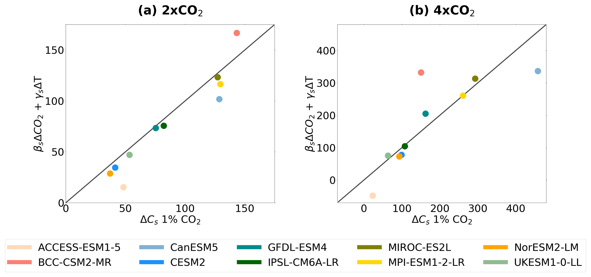
Figure 5 Comparison of ΔC_s (PgC) in the full 1 % CO₂ simulation (x axis) against the estimated ΔC_s using the calculated β_s and γ_s feedback parameters (y axis), where estimated $\mathrm{\Delta }{C}_{\mathrm{s}}\approx {\mathit{\beta }}_{\mathrm{s}}\mathrm{\Delta }{\mathrm{CO}}_{\mathrm{2}}+{\mathit{\gamma }}_{\mathrm{s}}\mathrm{\Delta }T$ for each CMIP6 ESM at (a) 2 × CO₂ and (b) 4 × CO₂.

It is apparent from Fig. 4 that the sensitivities of NPP and τ_s to both CO₂ and T must be accounted for to understand and quantify the sensitivities of soil carbon. The magnitude of β_τ is found to be approximately one-third of the magnitude of β_NPP at both 2 × CO₂ and 4 × CO₂ but with counteracting signs of change. Models with the lowest β_NPP sensitivities also see the lowest β_τ sensitivities (e.g. ACCESS-ESM1-5) and vice versa. The magnitude of γ_NPP is generally found to be greater across the ensemble compared with γ_τ, with however a greater range of sensitivities. Additionally, the apparent sensitivity of soil carbon to CO₂ is less than the individual sensitivities of NPP and τ_s, due to a cancellation effect from opposing signs, leading to a lower apparent β_s. The magnitudes of β_NPP and β_τ are lower at 4 × CO₂ than 2 × CO₂, which means a reduced sensitivity of NPP and τ_s to CO₂ at greater levels of climate change. However, due to this cancellation effect, the same reduced sensitivity is not seen in β_s. Conversely, a reduced sensitivity of NPP and τ_s to temperature is not suggested under increasing climate forcing. No clear relationship between γ_NPP and γ_τ is seen amongst the CMIP6 ESMs (Fig. 4).

The contribution of the non-linearity between NPP and τ_s to the net soil carbon sensitivity is also investigated (β_ΔNPPΔτ and γ_ΔNPPΔτ). Figure 4 suggests that the non-linearity between NPP and τ_s is more robustly projected to result from increasing CO₂ (β_s). However, non-linearities in γ_s are also seen in the models with the greatest temperature sensitivities. The ensemble mean predicted β_ΔNPPΔτ is found to be −0.462 ± 0.462 at 2 × CO₂ and −0.463 ± 0.468 PgC ppm⁻¹ at 4 × CO₂. As expected from Fig. 4, predicted γ_ΔNPPΔτ is found to have a low sensitivity, where the ensemble means of −0.374 ±  3.12 at 2 × CO₂ and −0.0478 ± 7.42 PgC °C⁻¹ at 4 × CO₂ are found. Additionally, the NEP terms (β_NEP and γ_NEP) are shown to contribute to both CO₂ and T sensitivities (Fig. 4), due to the disequilibrium of land carbon changes under 1 % increasing CO₂.

3.4 Investigating the robustness of the ΔC_s approximation

Projections of ΔC_s in ESMs in the full 1 % CO₂ simulation were compared with the estimated ΔC_s derived using Eq. (7), which uses the derived β_s and γ_s feedback parameters together with model-specific ΔT and estimates for ΔCO₂ (Fig. 5). This investigates the approximation that changes in the full 1 % CO₂ simulation are equal to the sum of changes in the BGC and RAD simulations. At 2 × CO₂, the approximation is found to predict ΔC_s within 20 % of the actual projected values in the 1 % CO₂ simulation for 7 out of the 10 CMIP6 ESMs (BCC-CSM2-MR, CESM2, GFDL-ESM4, IPSL-CM6A-LR, MIROC-ES2L, MPI-ESM1-2-LR and UKESM1-0-LL). At 4 × CO₂, the robustness of the assumption between the BGC and RAD simulations decreases for future changes in soil carbon. However, β_sΔCO₂+γ_sΔT is within 20 % of the projected ΔC_s for 5 out of the 10 ESMs (GFDL-ESM4, IPSL-CM6A-LR, MIROC-ES2L, MPI-ESM1-2-LR and UKESM1-0-LL). The models where the approximation is the least consistent with projected ΔC_s are ACCESS-ESM1-5 and BCC-CSM2-MR, where at 4 × CO₂ the greatest non-linearities are present between BGC and RAD simulations (Fig. 5).

3.5 Comparisons between soil and land feedback parameters

The contribution of the sensitivity of soil carbon stocks (C_s) to the total sensitivity of land carbon stocks (C_L) was investigated by comparing the β and γ feedback parameters for land (Table A1) and soil (Table 2) for both 2 × CO₂ and 4 × CO₂ in CMIP6 ESMs (Fig. 6). Here, the assumption from Eq. (5) is followed that the land sensitivity is made up of the sum of the soil and vegetation responses. For the carbon-concentration feedback (β), the portion of the land sensitivity to CO₂ (β_L) that is due to global soils (β_s) ranges from 19 % (NorESM2-LM) to 53 % (BCC-CSM2-MR), with a mean of 38 ± 11 % seen across the CMIP6 ESMs at 2 × CO₂ (Fig. 6a). Similar proportions are found at 4 × CO₂, ranging from 22 % (NorESM2-LM) to 58 % (MIROC-ES2-L), with a mean of 42 ± 12 % seen across the CMIP6 ESMs (Fig. 6b). The portion of β_L due to β_s is estimated to be close to half of the total land response. For the carbon-climate feedback (γ), the portion of the land sensitivity to climate (γ_L) that is due to global soils (γ_s) ranges from approximately 42 % (CESM2) to 147 % (MPI-ESM1-2-LM), with a mean of 75 ± 30  % seen across the CMIP6 ESMs at 2 × CO₂ (Fig. 6a), and at 4 × CO₂ the range is from 48 % (ACCESS-ESM1-5) to 157 % (MPI-ESM1-2-LM), with a mean of 75 ± 31  % seen across the CMIP6 ESMs (Fig. 6b). Therefore, the portion of γ_L due to γ_s is estimated to be the majority of the sensitivity, suggesting that soil dominates the response of land carbon to climate. Note that the MPI-ESM1-2-LR model sees a greater γ_s value compared with γ_L, resulting in the percentage of the land response attributed to soil being greater than 100 %. This suggests a positive γ_v response in this model, meaning a predicted increased vegetation carbon globally with global warming.

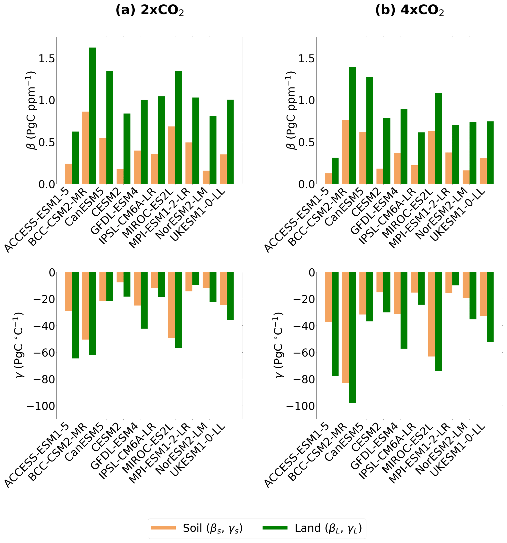
Figure 6 Comparisons of the land carbon-concentration (β_L) feedback parameters with the soil carbon-concentration (β_s) feedback parameters (top row) and the land carbon-climate (γ_L) feedback parameters with the soil carbon-climate (γ_s) feedback parameters (bottom row), for (a) 2 × CO₂ and (b) 4 × CO₂.

4 Discussion

Quantifying the future sensitivity of global soil carbon stocks to anthropogenic CO₂ emissions and their role in future land carbon storage is vital in order to understand future changes in the Earth's climate system (Canadell et al., 2021). Global changes in soil carbon (ΔC_s), in the absence of human disturbance and land-use change, will result from responses due to changes in atmospheric CO₂ and the associated changes in global temperatures (T), which are used to represent climate effects on a global scale. By separating the sensitivities due to increasing CO₂ and T, the idealised C4MIP ESM simulations allow for these effects on soil carbon to be examined individually, and the use of the βγ formulation allows these sensitivities to be quantified and compared for CMIP6 ESMs (Jones et al., 2016; Friedlingstein et al., 2006). Further, combining the βγ formulation with the Varney et al. (2023) ΔC_s framework allows us to isolate the sensitivities of soil carbon processes which influence β_s and γ_s within models.

Across CMIP6 ESMs, soil carbon is projected to increase in the BGC simulation (“CO₂-only”) and decrease in the RAD simulation (“climate-only”), consistent with projections of the overall land carbon response (Arora et al., 2020). The BGC simulation has been used to quantify the sensitivity of soil carbon to ΔCO₂ (β_s), where positive β_s values were defined according to the projected increase in soil carbon with increased atmospheric CO₂ (Fig. 1b). The positive β_s has been shown here to mostly be a result of a positive β_NPP term (Fig. 4), which represents the increased CO₂ fertilisation effect describing increased vegetation productivity under higher atmospheric CO₂ concentrations, which leads to an increased input of litter carbon into soil carbon pools (Schimel et al., 2015; Koven et al., 2015). A negative contribution of β_τ to β_s is also shown (Fig. 4). Previously, Varney et al. (2023) presented a transient reduction in τ_s in CMIP6 ESMs due to an increased rate of carbon input into the soil (i.e. negative β_τ due to positive β_NPP), a phenomenon known as false priming (Koven et al., 2015). However, it can be seen that the magnitude of this effect is small compared with the CO₂ fertilisation effect across the ESMs (β_τ vs. β_NPP, Fig. 4). Despite agreement on a net increase in soil carbon stocks globally (positive β_s), this study highlights uncertainty in the projected magnitude of this sensitivity amongst the CMIP6 models, which is seen to be driven by uncertainties in β_NPP (Fig. 4).

The RAD simulation has been used to quantify the sensitivity of soil carbon to changes in climate (ΔT; γ_s), where negative γ_s values were defined due to the projected decrease in soil carbon with global warming (Fig. 1c). The negative γ_s term has been shown here to be a result of negative γ_τ and, in many cases, negative γ_NPP (Fig. 4). The negative sensitivity of τ_s to global warming (negative γ_τ) is known to be due to an increased rate of heterotrophic respiration (R_h) at warmer temperatures as a result of increased microbial activity (Varney et al., 2020; Crowther et al., 2016). The global sensitivity of NPP to climate changes (γ_NPP) is less certain where both negative and positive values are seen across the CMIP6 ESMs (Fig. 4). This is likely due to more spatially varying responses, where the resultant ΔC_s can be seen in Fig. 2. For example, increased temperatures at northern latitudes could result in the northward expansion of boreal forests (Pugh et al., 2018), which would increase forest productivity and subsequently carbon storage in these regions. However, future changes in precipitation patterns could lead to regions with reduced soil moisture, which would conversely lead to reduced vegetation productivity and carbon uptake (Green et al., 2019). The uncertainties associated with projected spatial changes (γ_NPP), together with the uncertainties in the magnitude of carbon turnover times within the soil (γ_τ; Varney et al., 2020; Koven et al., 2017), result in uncertainties in the sensitivity of soil carbon to climate changes (γ_s) amongst the CMIP6 models.

This paper highlights the importance of soils within the land carbon response to global warming (Fig. 6). Despite the ΔC_s sensitivity to CO₂ dominating net soil carbon changes (β_s), it could be argued that the significance of the ΔC_s climate sensitivity (γ_s) will increase under more extreme levels of climate change. This is suggested by both a projected saturation of β_s and an increase in γ_s between 2 × CO₂ and 4 × CO₂ shown in the CMIP6 ensemble means (Table 2). The saturation, or reduced rate of increase, in β_s seen in CMIP6 is likely due to a limit of the CO₂ fertilisation effect, based on the reduced β_NPP values between 2 × CO₂ and 4 × CO₂ (Fig. 4). The rate of CO₂ fertilisation in the future is expected to be limited by nutrient availability (Wieder et al., 2015), which in CMIP6 is now more explicitly represented by the inclusion of an interactive nitrogen cycle in multiple models (see Table 1). This implementation is expected to limit the increased productivity from CO₂ fertilisation within ESMs (Davies-Barnard et al., 2020) and has previously been found to lower the magnitude of the land feedback parameters (Arora et al., 2020). However, it is noted that warming within the soil could accelerate nutrient mineralisation, which could result in a liberation of nitrogen due to increased microbial breakdown of plant litter, alleviating the nutrient limitation in plants (Todd-Brown et al., 2014).

Unlike the β_s parameter, the sensitivity of soil carbon to climate changes (γ_s) has been shown to increase with global warming in CMIP6. The greater γ_s values at 4 × CO₂ compared with 2 × CO₂ found here imply an increased rate of soil carbon loss under increased amounts of global warming (Table 2). Additionally, it could be hypothesised that limitations within CMIP6 ESMs in the representation of soil carbon and related processes could lead to a potential underestimation of γ_s. In Fig. 2, reductions in soil carbon stocks at the high northern latitudes are only seen in three models for the full 1 % CO₂ simulation (BCC-CSM2-MR, CESM2 and NorESM2-LM). Varney et al. (2022) find that these CMIP6 models represent quantities of northern-latitude carbon stocks most consistently with observational estimates, which could imply an increased likelihood of soil carbon loss from the northern latitudes based on consistency with observations. It is noted however that CESM2 and NorESM2-LM contain the same land surface model and so are expected to show similar results (Lawrence et al., 2019). Furthermore, the majority of ESMs do not include explicit representation of permafrost carbon (Burke et al., 2020). Including permafrost within ESMs would result in increased quantities of carbon within the soil known to be especially sensitive to global warming (increased γ_s), which currently are not included in the calculation of these feedbacks (Schuur et al., 2015).

The βγ formulation has many benefits in allowing the quantification and comparison of land and soil carbon feedbacks amongst ESMs. However, one limitation is due to ΔC_s not being consistently linear with increasing CO₂ and temperature (Fig. 3), so the parameter values depend on the point in time at which they are calculated (for example, 2 × CO₂ or 4 × CO₂). This has been shown to be due to non-linearities in the processes driving soil carbon feedbacks (Fig. 4), such as the discussed saturation of the CO₂ fertilisation effect (β_NPP; Wang et al., 2020) and additionally a known Q₁₀ dependence of heterotrophic (soil) respiration on temperature (γ_τ; Zhou et al., 2009).

Non-linearities between CO₂ and T responses are also known and have previously been shown within ESMs in the future land carbon responses (Schwinger et al., 2014; Zickfeld et al., 2011; Gregory et al., 2009). Zickfeld et al. (2011) suggest that the non-linearity in the land response is due to significantly differing vegetation responses which depend on whether or not climate effects are combined with the CO₂ fertilisation effect, e.g. forest dieback (Cox et al., 2004). However, this is model-dependent, as not all models within CMIP6 simulate dynamic vegetation (Table 1). The spatial variations in the response of soil carbon to CO₂ and climate that are seen in Fig. 2 could also contribute to the non-linearity. For example, a different spatial pattern of soil carbon under elevated CO₂ could lead to a different overall temperature response, e.g. if more carbon is at the high latitudes where greater temperature changes are seen. Arora et al. (2020) find that climate responses in the BGC simulation account for a difference of 1 %–5 % in the calculation of the feedbacks, suggesting a small but non-negligible effect of climate in the BGC runs. This response was shown to be dependent on the representation of vegetation within the model, as with the non-linearities found in Zickfeld et al. (2011). Despite this, isolating and quantifying the key sensitivities with the βγ method provides a useful benchmark for feedbacks within CMIP.

5 Conclusions

The Friedlingstein et al. (2006) methodology adapted in this study suggests that β_s and γ_s linearity is a valid assumption for projected soil carbon changes in ESMs up until a doubling of CO₂. However, under more extreme levels of climate change, the results here suggest the need for the non-linearity in feedbacks to be further investigated. Soil carbon is found to have a greater impact on carbon-climate feedbacks than vegetation carbon responses, which means that the sensitivity of soil carbon to changes in global temperature is the dominant response of the land carbon cycle when considering climate effects. Therefore, further understanding and quantifying the sensitivity of global soils under global warming is necessary to quantify future changes in the climate system. Moreover, the sensitivity of soil carbon to temperature increases with increasing climate forcing, suggesting that soil carbon is particularly important in the long-term land carbon response under extreme levels of global warming.

Appendix A

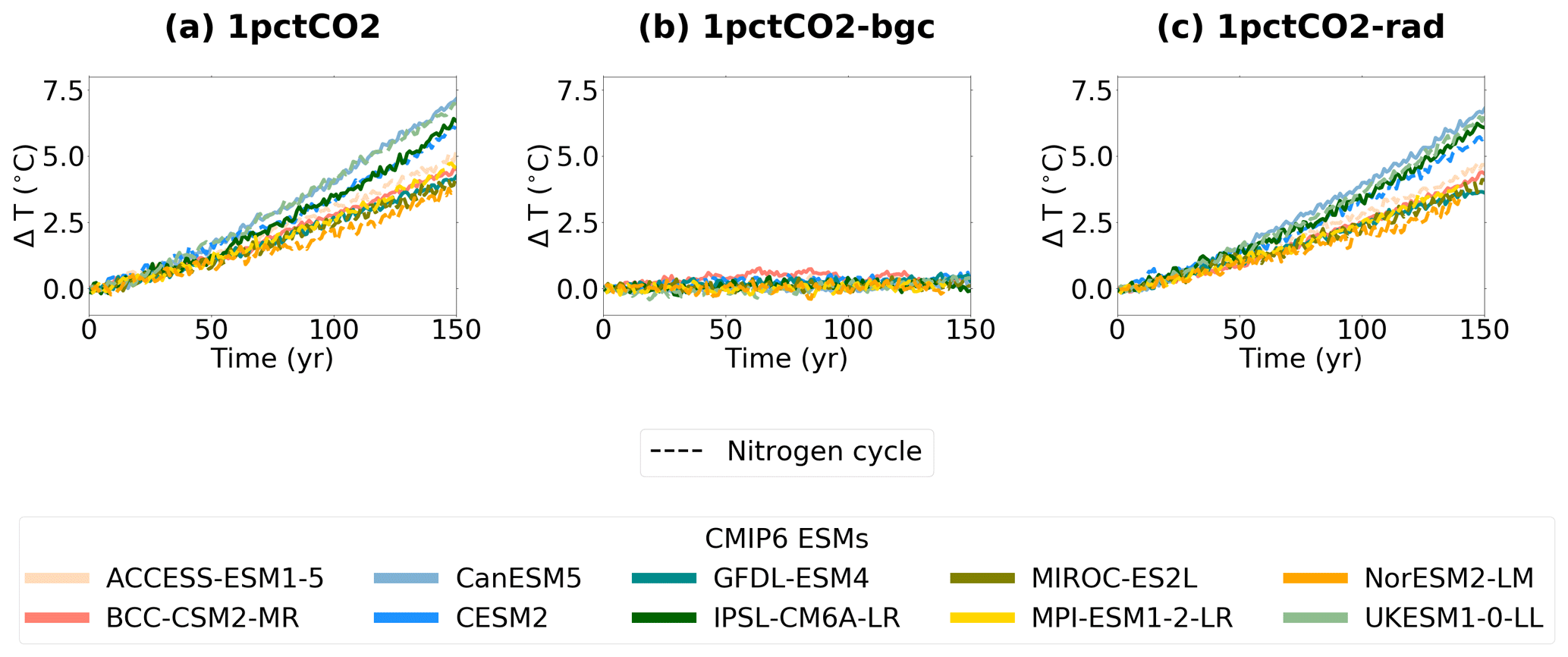
Figure A1 Time series of projected global mean temperature changes (ΔT) in CMIP6 ESMs for the idealised simulations 1 % CO₂ (a), biogeochemically coupled 1 % CO₂ (BGC, b) and radiatively coupled 1 % CO₂ (RAD, c).

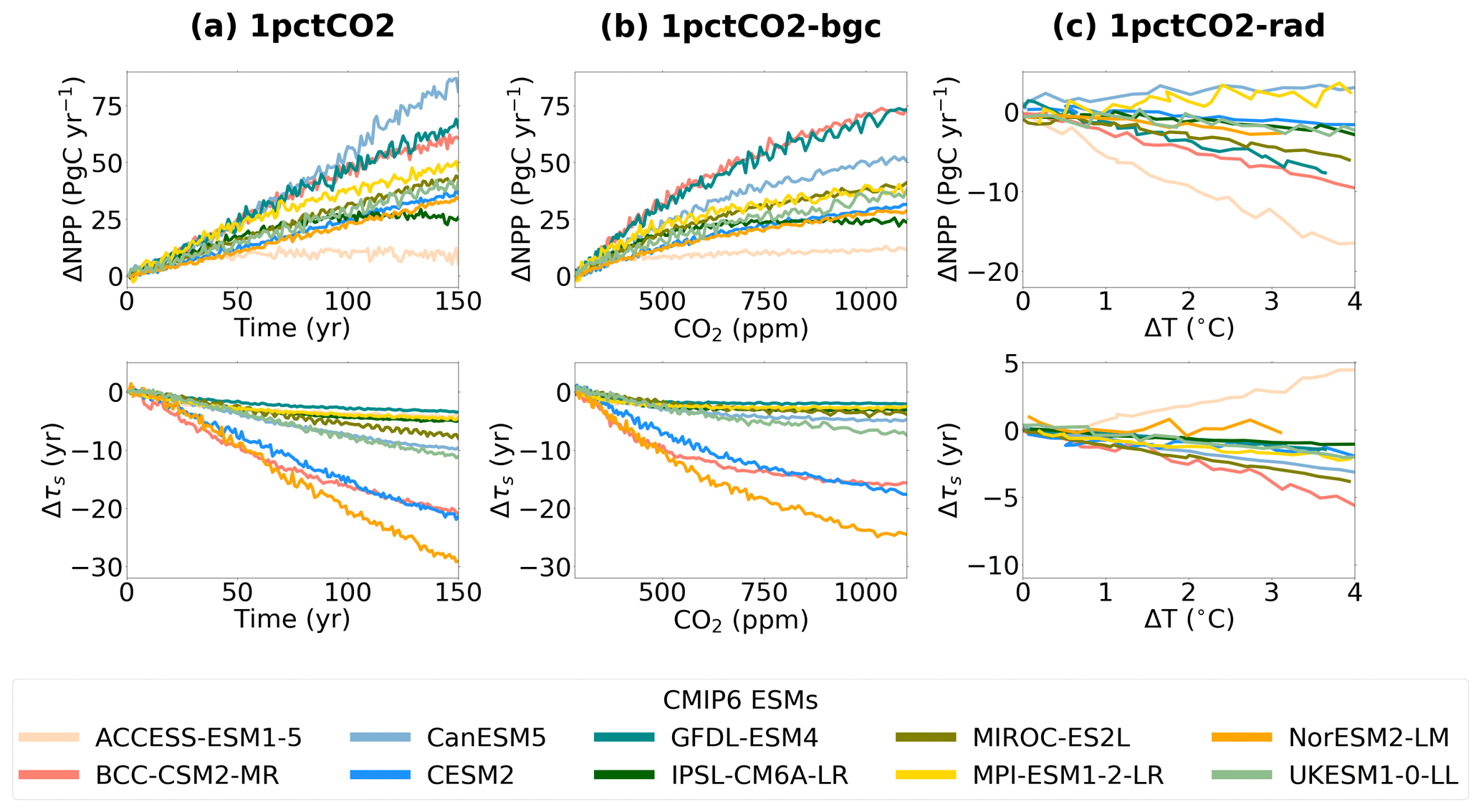
Figure A2 Time series of projected changes in net primary productivity (ΔNPP, top row) and soil carbon turnover time (Δτ_s, bottom row) in CMIP6 ESMs for the idealised simulations 1 % CO₂ (a), BGC (b) and RAD (c). This figure has been adapted from Fig. A2 in Varney et al. (2023).

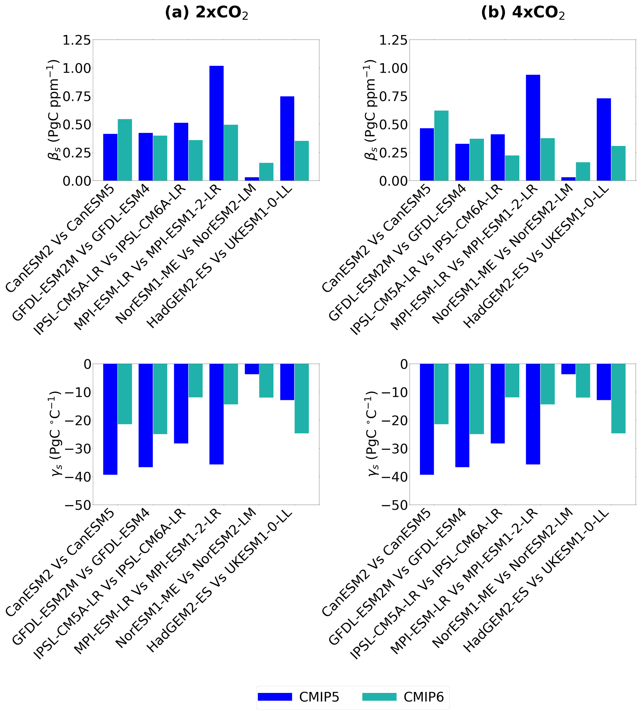
Figure A3 Comparison of the soil carbon-concentration (β_s) feedback parameters (top row) and the soil carbon-climate (γ_s) feedback parameters (bottom row) from generationally related ESMs from CMIP5 and CMIP6, for (a) 2 × CO₂ and (b) 4 × CO₂.

Table A1 The land carbon-concentration (β_L, PgC ppm⁻¹) and carbon-climate (γ_L, PgC °C⁻¹) feedback parameters for 2 × CO₂ and 4 × CO₂ for the CMIP6 ESMs.

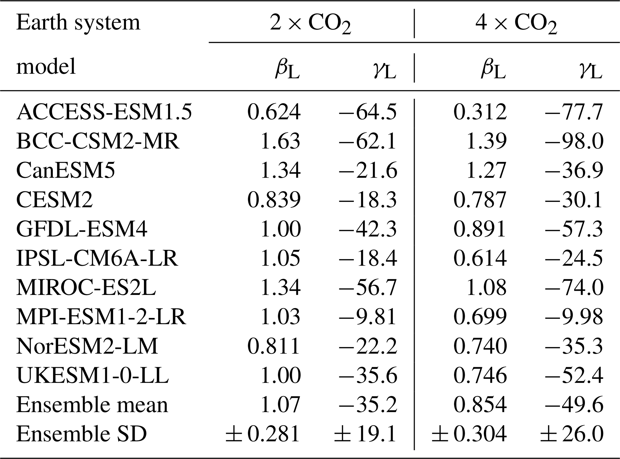
Table A2 The CMIP5 Earth system models included in this study and the relevant features of the associated land carbon cycle components: simulation of interactive nitrogen, the inclusion of dynamic vegetation and the soil decomposition functions used (Varney et al., 2022; Arora et al., 2013; Anav et al., 2013; Friedlingstein et al., 2014). Explanations of the temperature and moisture functions used within ESMs are given in Varney et al. (2022) and Todd-Brown et al. (2013).

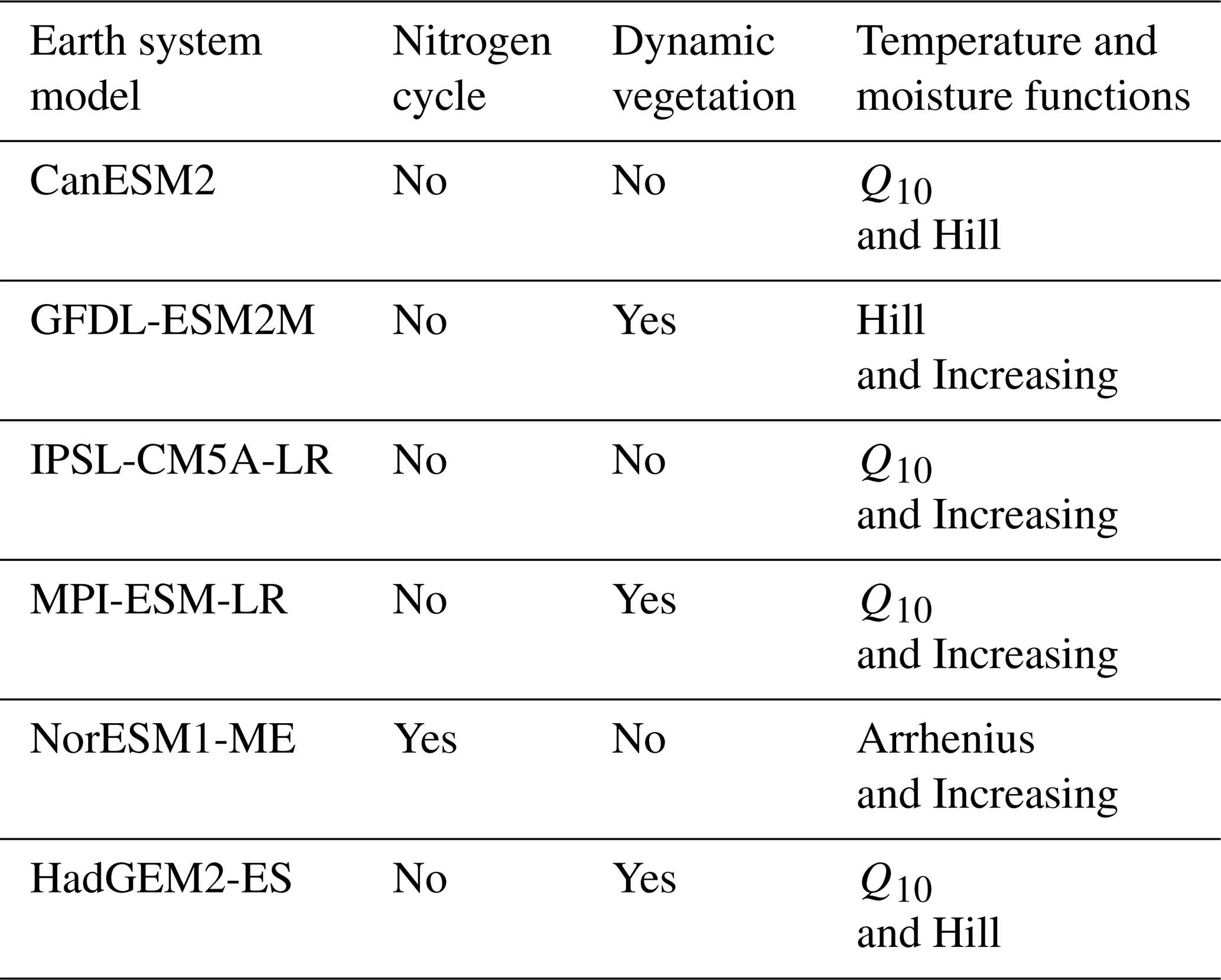
Table A3 The soil carbon-concentration (β_s, PgC ppm⁻¹) and carbon-climate (γ_s, PgC °C⁻¹) feedback parameters for 2 × CO₂ and 4 × CO₂ for the CMIP5 ESMs.