Simulated responses of soil carbon to climate change in CMIP6 Earth system models: the role of false priming

Reliable estimates of soil carbon change are required to determine the carbon budgets consistent with the Paris Agreement climate targets. This study evaluates projections of soil carbon during the 21st century in Coupled Model Intercomparison Project Phase 6 (CMIP6) Earth system models (ESMs) under a range of atmospheric composition scenarios. In general, we find a reduced spread of changes in global soil carbon (ΔC_s) in CMIP6 compared to the previous CMIP5 model generation. However, similar reductions were not seen in the derived contributions to ΔC_s due to both increases in plant net primary productivity (NPP, named ΔC_s,NPP) and reductions in the effective soil carbon turnover time (τ_s, named ΔC_s,τ). Instead, we find a strong relationship across the CMIP6 models between these NPP and τ_s components of ΔC_s, with more positive values of ΔC_s,NPP being correlated with more negative values of ΔC_s,τ. We show that the concept of “false priming” is likely to be contributing to this emergent relationship, which leads to a decrease in the effective soil carbon turnover time as a direct result of NPP increase and occurs when the rate of increase in NPP is relatively fast compared to the slower timescales of a multi-pool soil carbon model. This finding suggests that the structure of soil carbon models within ESMs in CMIP6 has likely contributed towards the reduction in the overall model spread in future soil carbon projections since CMIP5.

1 Introduction

The response of soil carbon to human-induced climate change represents one of the greatest uncertainties in determining future atmospheric CO₂ concentrations (Canadell et al., 2021). Global soil carbon stocks contain at least 3 times more carbon than present atmospheric concentrations and are the largest store of carbon on the land surface of Earth (Jackson et al., 2017). The land surface has been a carbon sink throughout the 20th century and is estimated to be absorbing about 30 % of current CO₂ emissions (Friedlingstein et al., 2022). However, the long-term response of soil carbon is uncertain due to large stocks which are known to be particularly sensitive to changes in CO₂ and the subsequent global warming (Cox et al., 2000). For example, permafrost thaw under climate change has the potential to release significant amounts of carbon into the atmosphere over a short period of time with increased warming, representing a significant feedback within the climate system (Schuur et al., 2022; Hugelius et al., 2020; Burke et al., 2017). Therefore, quantifying the future response of soil carbon under future changes to climate is vital in determining the long-term potential land carbon storage.

Soil carbon storage in the future will be determined by the net response of changes in land–atmosphere carbon exchange under increased anthropogenic CO₂. The carbon fluxes which control the fate of global soil carbon stocks are known to be sensitive to changes in climate and therefore result in soil-carbon-driven feedbacks to climate change (Canadell et al., 2021). The overall effect of climate change on soil carbon is not very well constrained due to competing feedbacks (Arora et al., 2020, 2013). These include both the negative feedback due to the CO₂ fertilisation effect, resulting in increased absorption of carbon by the land surface (Schimel et al., 2015), and the positive climate feedback due to increased carbon losses via soil respiration (Crowther et al., 2016; Van Gestel et al., 2018). The balance between these effects will determine the future response of soil carbon stocks under a changing climate (Friedlingstein et al., 2006).

This study assumes that net primary productivity (NPP) represents the input flux of carbon to the system and is defined as the net rate of accumulation of carbon by vegetation arising from photosynthesis minus the loss from plant respiratory fluxes (Todd-Brown et al., 2014, 2013). In the absence of nutrient and moisture limitations (Wieder et al., 2015b; Green et al., 2019), NPP is projected to increase under increased atmospheric CO₂ due to the CO₂ fertilisation effect, which can result in increased soil carbon storage through increased litter (Schimel et al., 2015). Heterotrophic respiration (R_h) is assumed to represent the output flux of carbon from the soil and is defined as the carbon losses due to decomposition from microbes in the soil. R_h is projected to increase under global warming due to an increased rate of microbial decomposition under warming (Varney et al., 2020) in the absence of significant increases in soil moisture (Sierra et al., 2015; Schmidt et al., 2011). Soil carbon turnover time (τ_s) is defined as the ratio of soil carbon stocks to the output flux of carbon (R_h). Global warming alone generally reduces τ_s, resulting in carbon residing in the soil for less time and a release of carbon from the soil into the atmosphere (Crowther et al., 2016). The effective soil carbon turnover time can also reduce under increasing litterfall inputs (e.g. due to CO₂ fertilisation of plant growth), because the faster components of the soil increase more quickly than the slower components. The net effect of this is that a higher fraction of the soil carbon flux is cycled in the fast pools under increasing litterfall, which reduces the effective soil carbon turnover time – a transient phenomenon known as false priming (Koven et al., 2015).

In this study, CMIP6 Earth system models (ESMs) are used to predict changes to soil carbon stocks under future climate scenarios with differing magnitudes of climate change (SSP126, SSP245, SSP585; Eyring et al., 2016; O'Neill et al., 2016). The aim is to evaluate estimates of soil carbon change (ΔC_s) during the 21st century to (a) quantify the soil-carbon-driven feedback to climate change and (b) enable comparisons with the previous generation of CMIP5 ESMs (RCP2.6, RCP4.5, RCP8.5; Taylor et al., 2012; Meinshausen et al., 2011). Additionally, this study includes analysis of 21st century carbon fluxes to and from the soil, represented by changes in NPP and τ_s, and investigates how these individual terms contribute to the net soil carbon response projected by ESMs. Finally, a simple box model is used to investigate soil carbon change, along with idealised simulations (Coupled Climate-Carbon Cycle Model Intercomparison Project – C4MIP) which separately model the physiological and climate effects of increasing atmospheric CO₂. Our aim is to distinguish more clearly between the direct and indirect mechanisms of reduced soil carbon turnover times by isolating the effects of false priming in models.

2 Methods

2.1 Earth system models

2.1.1 Future climate scenarios

This study uses output data from 10 CMIP6 ESMs (Eyring et al., 2016): ACCESS-ESM1-5, BCC-CSM2-MR, CanESM5, CESM2, CNRM-ESM2-1, IPSL-CM6A-LR, MIROC-ES2L, MPI-ESM1-2-LR, NorESM2-LM, and UKESM1-0-LL. For comparison between the CMIP generations, output data from nine CMIP5 ESMs are also used (Taylor et al., 2012): BNU-ESM, CanESM2, GFDL-ESM2G, GISS-E2-R, HadGEM2-ES, IPSL-CM5A-LR, MIROC-ESM, MPI-ESM-LR, and NorESM1-M. The ESMs included were chosen due to the availability of the data required at the time of analysis (CMIP6: https://esgf-node.llnl.gov/search/cmip6/, last access: 8 April 2022; CMIP5: https://esgf-node.llnl.gov/search/cmip5/, last access: 12 April 2022).

Ji et al. (2014); Dai et al. (2003)Arora et al. (2009); Arora and Boer (2010)Dunne et al. (2012, 2013)Shevliakova et al. (2009)Schmidt et al. (2014); Yue and Unger (2015)Jones et al. (2011); Best et al. (2011)Clark et al. (2011)Dufresne et al. (2013); Krinner et al. (2005)Watanabe et al. (2011); Ito and Oikawa (2002)Sato et al. (2007)Raddatz et al. (2007); Knorr (2000)Bentsen et al. (2013); Iversen et al. (2013)Lawrence et al. (2011)Ziehn et al. (2020); Haverd et al. (2018)Wu et al. (2019); Ji et al. (2008)Swart et al. (2019); Melton et al. (2020)Seiler et al. (2021)Danabasoglu et al. (2020); Lawrence et al. (2019)Séférian et al. (2019); Delire et al. (2020)Dunne et al. (2020); Zhao et al. (2018)Boucher et al. (2020); Cheruy et al. (2020)Guimberteau et al. (2018)Hajima et al. (2020); Ito and Oikawa (2002)Mauritsen et al. (2019); Goll et al. (2017)Goll et al. (2015)Seland et al. (2020); Lawrence et al. (2019)Sellar et al. (2020); Wiltshire et al. (2021)

Table 1 The CMIP5 and CMIP6 Earth system models included in this study and the relevant features of the associated land carbon cycle components: simulation of interactive nitrogen, the number of live carbon pools, and the number of dead soil carbon pools (Varney et al., 2022; Arora et al., 2013, 2020).

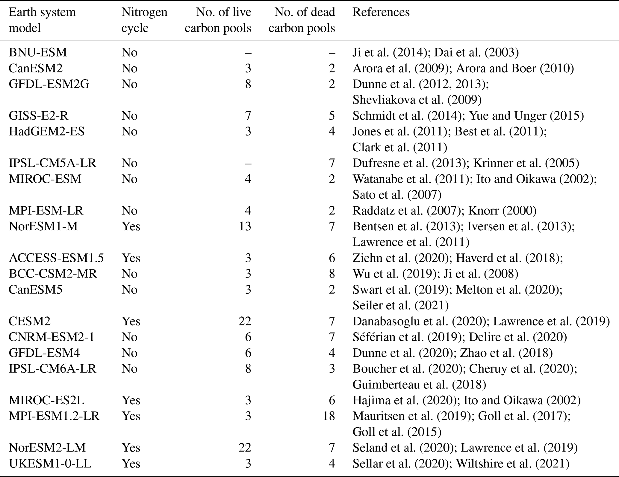
The use of CMIP allows for comparison between ESMs in the different ensemble generations. Table 1 presents key soil carbon ESM information from both CMIP6 and CMIP5 (adapted from Tables 1 and 2 in Varney et al., 2022). The table can be used to identify key ESM updates between CMIP6 and CMIP5, such as the simulation of interactive nitrogen in CMIP6 (ACCESS-ESM1.5, CESM2, MIROC-ES2L, MPI-ESM1.2-LR, NorESM2-LM, and UKESM1-0-LL) compared to CMIP5 (NorESM1-M) and the number of soil carbon pools (dead carbon pools). The ESMs where both CMIP5 and CMIP6 generations are included in our analysis are CanESM2 and CanESM5, GFDL-ESM2G and GDFL-ESM4, IPSL-CM5A-LR and IPSL-CM6A-LR, MIROC-ESM and MIROC-ES2L, MPI-ESM-LR and MPI-ESM1.2-LR, NorESM1-M and NorESM2-LM, and HadGEM2-ES and UKESM1-0-LL, respectively, where direct comparisons can be made. It is noted that some land surface models within ESMs share similarities (e.g. CESM2 and NorESM2-LM both use the Community Land Model version 5; Arora et al., 2020).

Within ESMs, specific soil carbon processes are modelled using biogeochemical models which are used to simulate the flow and storage of carbon within the soil. Since early models, both the litter and soil have been simulated using separate carbon pools, which are used to represent differing sensitivities of carbon to decomposition. The allocation of carbon to pools is often dependent on the molecular structure of the litter and the long-term stability (Exbrayat et al., 2013). Early examples of soil carbon models are the grass and agroecosystems dynamic model (CENTURY; Parton et al., 1988) and the Rothamsted carbon model (ROTH-C; Jenkinson et al., 1991). Updated variants of these models are still widely used to represent soil carbon decomposition in modern ESMs within CMIP (Arora et al., 2020; Todd-Brown et al., 2018). Table 1 presents the number of soil carbon pools (dead carbon pools) within both CMIP5 and CMIP6 ESMs, which can be used to compare between the ESMs.

The analysis in this study considers three future climate scenarios defined by CMIP, which are used to consider different levels of global warming and the associated climate policies. The CMIP6 shared socioeconomic pathways (SSPs) considered in this study are SSP126, SSP245, and SSP585, which run from 2015 to 2100 (O'Neill et al., 2014, 2016). These pathways are chosen to allow for comparison with the CMIP5 representative concentration pathways (RCPs) RCP2.6, RCP4.5, and RCP8.5, which run from 2005 to 2100 (Meinshausen et al., 2011). It is noted that the SSP and RCP concentration scenarios are not identical, but they are similar enough to enable helpful comparisons between CMIP5 and CMIP6 projections. For the reference period from which change is calculated, the CMIP Historical simulation was considered, where the simulation runs from 1850 to 2005 in CMIP5 and from 1850 to 2015 in CMIP6. A change (Δ) was defined as the difference between the last decade of the 21st century (time-averaged between 2090 and 2100) and the last decade of the CMIP5 historical simulation (time-averaged between 1995 and 2005), which allows for consistency between the CMIP generations. If a time series is considered, the historical reference period (historical simulation time-averaged between 1995 and 2005) was subtracted from the entire future climate simulation (e.g. SSP126 minus the historical reference period).

2.1.2 C4MIP experiments

This study also uses model experiments set up by C4MIP that are idealised experiments designed to separate the effects of CO₂ increases and associated climate changes on land and ocean carbon stores. In these experiments additional effects such as land use change, aerosols, or non-CO₂ greenhouse gases are not included, and nitrogen deposition is fixed at pre-industrial values (Jones et al., 2016). The use of these experiments allows for a more focused evaluation of soil carbon and related fluxes by isolating sensitivities to CO₂ and associated climate changes (e.g. global temperature changes) and removing additional complications in the SSP simulations. The experiments included are (1) a full 1 % CO₂ simulation (CMIP6 simulation 1pctCO2), which is a simulation that sees a 1 % increase in atmospheric CO₂ per year, starting from pre-industrial concentrations (285 ppm) and running for 150 years (full 1 % CO₂); (2) a biogeochemically coupled BGC simulation (CMIP6 simulation 1pctCO2-bgc), where the 1 % CO₂ increase per year only affects the carbon cycle component of the ESM and the radiative code remains at pre-industrial CO₂ values (CO₂ only); and (3) a radiatively coupled RAD simulation (CMIP6 simulation 1pctCO2-rad), where the 1 % CO₂ increase per year affects only the radiative code and the carbon cycle component on the ESM remains at pre-industrial CO₂ values (climate only). These simulations are used with 10 CMIP6 ESMs for further analysis: ACCESS-ESM1-5, BCC-CSM2-MR, CanESM5, CESM2, GFDL-ESM4, IPSL-CM6A-LR, MIROC-ES2L, MPI-ESM1-2-LR, NorESM2-LM, and UKESM1-0-LL. Here, 2 × CO₂ and 4 × CO₂ are defined as 70 and 140 years, respectively, into the simulations.

2.1.3 Climate variables

Using ESM output variables, soil carbon (C_s) is defined as the sum of carbon stored in soils and surface litter (CMIP variable cSoil + CMIP variable cLitter). This allows for a more consistent comparison between the models due to differences in how soil carbon and litter carbon are defined. For models that do not report a separate litter carbon pool (cLitter), soil carbon is taken to be simply the cSoil variable (UKESM1-0-LL in CMIP6, GISS-E2-R and HadGEM2-ES in CMIP5). Spatial C_s is given in units of kilogram per square metre (kg m⁻²), and global total C_s is given in units of petagrams of carbon (PgC), which are calculated using an area-weighted sum (using the model land surface fraction, CMIP variable sftlf).

Additionally, ESM output variables were used to define the soil-carbon-driven climate feedbacks. NPP (CMIP variable npp) is defined as the net carbon assimilated by plants via photosynthesis minus loss due to plant respiration and is used to represent the net carbon input flux to the system. R_h (CMIP variable rh) is defined as the microbial respiration within global soils and is used to define an effective global soil carbon turnover time (τ_s): see Eq. (1). τ_s (years) is defined as the ratio of mean soil carbon to annual mean heterotrophic respiration (where the mean represents an area-weighted global average). Carbon fluxes (NPP and R_h) are considered as area-weighted global totals (Pg C yr⁻¹).

$$\begin{array}{}\text{(1)}& {\mathit{\tau }}_{\mathrm{s}}={\displaystyle \frac{{\mathrm{C}}_{\mathrm{s}}}{R_{\mathrm{h}}}}\end{array}$$

2.2 Breaking down the projected changes in soil carbon

From Eq. (1), soil carbon (C_s) can be defined as shown by Eq. (2). Future soil carbon stocks can be defined as initial soil carbon (C_s,0) plus a change in soil carbon (ΔC_s) as shown by Eq. (3), where the subscript 0 denotes the initial state (historical simulation time-averaged between 1995 and 2005). Equation (3) can be expanded to give Eq. (4), which can be simplified to give Eq. (5).

$$\begin{array}{}\text{(2)}& {\displaystyle }{\mathrm{C}}_{\mathrm{s}}=R_{\mathrm{h}}{\mathit{\tau }}_{\mathrm{s}}\text{(3)}& {\displaystyle }{\mathrm{C}}_{\mathrm{s},\mathrm{0}}+\mathrm{\Delta }{\mathrm{C}}_{\mathrm{s}}=(R_{\mathrm{h},\mathrm{0}}+\mathrm{\Delta }{R}_{\mathrm{h}})({\mathit{\tau }}_{\mathrm{s},\mathrm{0}}+\mathrm{\Delta }{\mathit{\tau }}_{\mathrm{s}})\text{(4)}& {\displaystyle }\begin{array}{rl}{\mathrm{C}}_{\mathrm{s},\mathrm{0}}+\mathrm{\Delta }{\mathrm{C}}_{\mathrm{s}}=& R_{\mathrm{h},\mathrm{0}}{\mathit{\tau }}_{\mathrm{s},\mathrm{0}}+{\mathit{\tau }}_{\mathrm{s},\mathrm{0}}\mathrm{\Delta }{R}_{\mathrm{h}}+R_{\mathrm{h},\mathrm{0}}\mathrm{\Delta }{\mathit{\tau }}_{\mathrm{s}}\\ & +\mathrm{\Delta }{R}_{\mathrm{h}}\mathrm{\Delta }{\mathit{\tau }}_{\mathrm{s}}\end{array}\text{(5)}& {\displaystyle }\mathrm{\Delta }{\mathrm{C}}_{\mathrm{s}}={\mathit{\tau }}_{\mathrm{s},\mathrm{0}}\mathrm{\Delta }{R}_{\mathrm{h}}+R_{\mathrm{h},\mathrm{0}}\mathrm{\Delta }{\mathit{\tau }}_{\mathrm{s}}+\mathrm{\Delta }{R}_{\mathrm{h}}\mathrm{\Delta }{\mathit{\tau }}_{\mathrm{s}}\end{array}$$

To isolate the above- and below-ground effects on soil carbon, the separate effects due to changes in NPP and changes due to τ_s are considered (Todd-Brown et al., 2014). For carbon to be conserved, however, the difference between the global fluxes NPP and R_h in a transient climate must be taken into account, where the difference is defined as the net ecosystem productivity (NEP), as shown in Eq. (6).

$$\begin{array}{}\text{(6)}& \mathrm{NEP}=\mathrm{NPP}-R_{\mathrm{h}}\end{array}$$

Equation (6) can be substituted into Eq. (5) to obtain an equation for ΔC_s in terms of NPP, NEP, and τ_s (Eq. 7).

$$\begin{array}{}\text{(7)}& \begin{array}{rl}\mathrm{\Delta }{\mathrm{C}}_{\mathrm{s}}=& {\mathit{\tau }}_{\mathrm{s},\mathrm{0}}\mathrm{\Delta }(\mathrm{NPP}-\mathrm{NEP})+({\mathrm{NPP}}_{\mathrm{0}}-{\mathrm{NEP}}_{\mathrm{0}})\mathrm{\Delta }{\mathit{\tau }}_{\mathrm{s}}\\ & +\mathrm{\Delta }(\mathrm{NPP}-\mathrm{NEP})\mathrm{\Delta }{\mathit{\tau }}_{\mathrm{s}}\end{array}\end{array}$$

If the initial state is a steady state, the initial NEP (NEP₀) will be approximately equal to zero. However, as our initial state is defined as the end of the historical simulation, NEP₀ will be non-zero as a result of the contemporary global land carbon sink. ESMs may also include additional carbon fluxes that cause changes to the resultant soil carbon inputs, such as grazing, harvest, land use change, and fire (Todd-Brown et al., 2014). The ΔNEP terms in Eq. (7) implicitly include these effects.

Finally, Eq. (7) can be expanded to give Eq. (8), and the individual responses which make up the total change in soil carbon (ΔC_s) can be broken down into six components:

$$\begin{array}{}\text{(8)}& \begin{array}{rl}\mathrm{\Delta }{\mathrm{C}}_{\mathrm{s}}=& {\mathit{\tau }}_{\mathrm{s},\mathrm{0}}\mathrm{\Delta }\mathrm{NPP}-{\mathit{\tau }}_{\mathrm{s},\mathrm{0}}\mathrm{\Delta }\mathrm{NEP}+{\mathrm{NPP}}_{\mathrm{0}}\mathrm{\Delta }{\mathit{\tau }}_{\mathrm{s}}\\ & -{\mathrm{NEP}}_{\mathrm{0}}\mathrm{\Delta }{\mathit{\tau }}_{\mathrm{s}}+\mathrm{\Delta }\mathrm{NPP}\mathrm{\Delta }{\mathit{\tau }}_{\mathrm{s}}-\mathrm{\Delta }\mathrm{NEP}\mathrm{\Delta }{\mathit{\tau }}_{\mathrm{s}}.\end{array}\end{array}$$

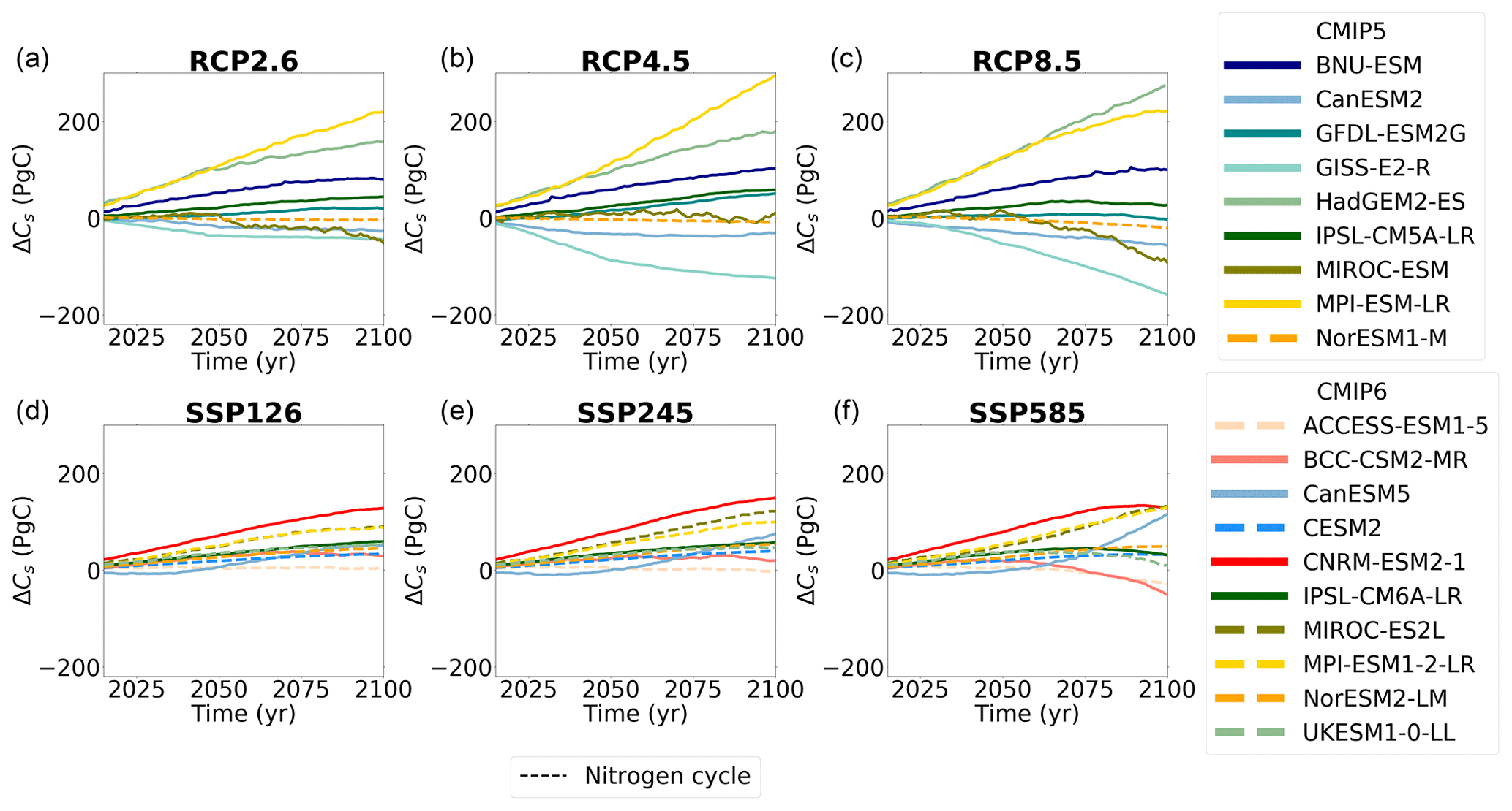
Figure 1 Projected future change in soil carbon (ΔC_s) in CMIP5 (a–c) and CMIP6 (d–f) ESMs for future climate scenarios RCP2.6 and SSP126, RCP4.5 and SSP245, and RCP8.5 and SSP585, respectively. The dashed lines represent ESMs which include the representation of interactive nitrogen in these simulations.

Equation (7) is exact for given time-varying values of NPP, NEP, and τ_s. The individual terms in Eq. (8) are defined as given below:

$$\begin{array}{}\text{(9)}& {\displaystyle }\mathrm{\Delta }{\mathrm{C}}_{\mathrm{s},\mathrm{NPP}}\approx {\mathit{\tau }}_{\mathrm{s},\mathrm{0}}\mathrm{\Delta }\mathrm{NPP},\text{(10)}& {\displaystyle }\mathrm{\Delta }{\mathrm{C}}_{\mathrm{s},\mathrm{NEP}}\approx -{\mathit{\tau }}_{\mathrm{s},\mathrm{0}}\mathrm{\Delta }\mathrm{NEP},\text{(11)}& {\displaystyle }\mathrm{\Delta }{\mathrm{C}}_{\mathrm{s},\mathit{\tau }}\approx {\mathrm{NPP}}_{\mathrm{0}}\mathrm{\Delta }{\mathit{\tau }}_{\mathrm{s}},\text{(12)}& {\displaystyle }\mathrm{\Delta }{\mathrm{C}}_{\mathrm{s},{\mathit{\tau }}_{\mathrm{NEP}}}\approx -{\mathrm{NEP}}_{\mathrm{0}}\mathrm{\Delta }{\mathit{\tau }}_{\mathrm{s}},\end{array}$$

where ΔC_s,NPP is the change in soil carbon due to changes in NPP, ΔC_s,NEP is the change in soil carbon due to changes in NEP, and ΔC_s,τ is the change in soil carbon due to changes in τ_s (with $\mathrm{\Delta }{\mathrm{C}}_{\mathrm{s},{\mathit{\tau }}_{\mathrm{NEP}}}$ accounting for non-equilibrium). The two additional terms are the non-linear term between NPP and τ_s (ΔNPPΔτ_s) and the non-linear term between NEP and τ_s (ΔNEPΔτ_s).

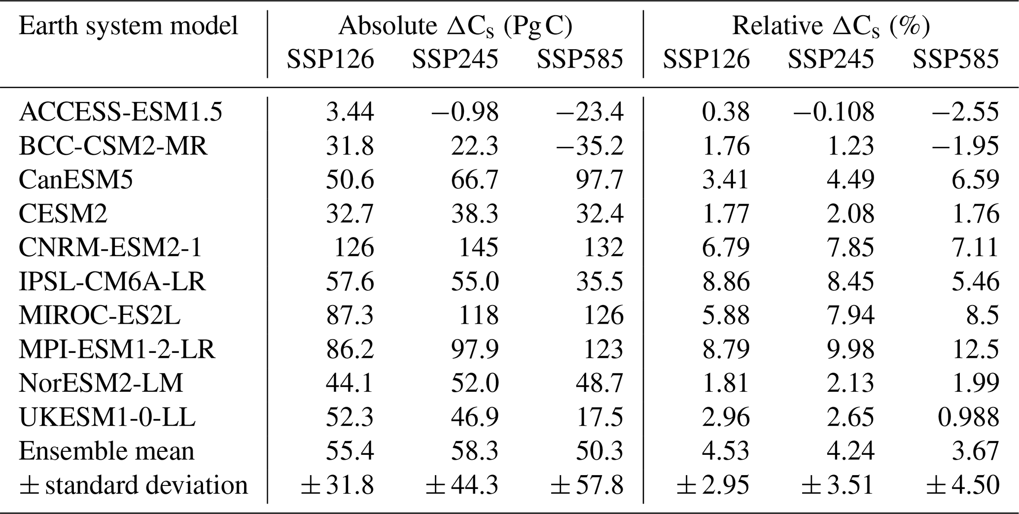
Table 2 Table presenting the absolute (Pg C) and relative (%) changes in 21st century soil carbon (ΔC_s) for each CMIP6 model and the ensemble mean ± standard deviation for each future SSP scenario.

3 Results and discussion

3.1 Projected changes in soil carbon

A reduced spread in projected end-of-21st-century estimates of ΔC_s is seen in CMIP6 compared to CMIP5 (Fig. 1). This reduced spread is shown in Fig. 1, where projections of ΔC_s by 2100 in CMIP6 are compared with those from CMIP5 across the different future scenarios. The reduced range of projected changes is seen across all future scenarios (SSP126 and RCP2.6, SSP245 and RCP4.5, SSP585 and RCP8.5), with the range in CMIP6 consistently less than 50 % of the equivalent range in CMIP5 (Fig. 1). The standard deviation of projections about the ensemble mean ΔC_s is also reduced in CMIP6 compared with CMIP5 by 50 %, consistent across all future climate scenarios (Tables 2 and A1, bottom rows). It is noted that the large range in CMIP5 estimates is mostly a result of large increases in C_s in HadGEM2-ES and MPI-ESM-LR together with the large C_s losses in GISS-E2-R (Fig. 1). An updated CMIP6 version of the GISS-E2-R model is not included in this analysis of this study, which could contribute to the reduced uncertainty from CMIP5. However, the updated equivalent CMIP6 models UKESM1-0-LL (from HadGEM2-ES) and MPI-ESM1-2-LR (from MPI-ESM-LR) have projected estimates of ΔC_s which are more consistent with the other models in the CMIP6 ensemble.

Nearly all of the ESM projections in CMIP6 suggest an increase in C_s by 2100; however, CMIP5 models project both increases (positive ΔC_s) and decreases (negative ΔC_s) in soil carbon during the 21st century (Fig. 1). In CMIP5 projections, the future responses of soil carbon range from an increase of 23.2 % (HadGEM2-ES) to a decrease of 6.50 % (GISS-E2-R) in RCP8.5, where across all future scenarios approximately half of the models show increases and half show decreases in ΔC_s (Table A1). In CMIP6, the future responses of soil carbon range from an increase of 12.5 % (MPI-ESM1-2-LR) to a decrease of 2.25 % (ACCESS-ESM1.5) in SSP585; however, the majority of the models predict an increase in ΔC_s across all the future scenarios (Table 2).

Despite more consistent projections of increased ΔC_s in CMIP6 compared with CMIP5, it is apparent that greater CO₂ forcing (i.e. SSP585 compared with SSP126) does not always imply a greater magnitude of increased C_s. In contrast to what is seen in CMIP6, the majority of CMIP5 models project an increased magnitude in estimated ΔC_s with increased CO₂ forcing (Fig. 1). In CMIP6, half the models (CESM2, CNRM-ESM2-1, IPSL-CM6A-LR, NorESM2-LM, and UKESM1-0-LL) estimate less soil carbon accumulation by 2100 (i.e. a smaller increase or a greater decrease) in SSP585 when compared with SSP126. This effect is most prominent in BCC-CSM2-MR and UKESM1-0-LL, where a turning point from increasing to decreasing soil carbon is seen in the mid-century of the SSP585 projections (Fig. 2). This is contrary to an estimated increase in soil carbon storage with increased forcing, which is generally seen in CMIP5 and the remaining CMIP6 models (CanESM5, MIROC-ES2L, and MPI-ESM1-2-LR). This finding is likely due to a saturation of the CO₂ fertilisation effect compared with no saturation of increased respiration with warming in these ESMs. This finding suggests a potential limit to ΔC_s increase and a reduced likelihood of a carbon sink under more extreme levels of climate change.

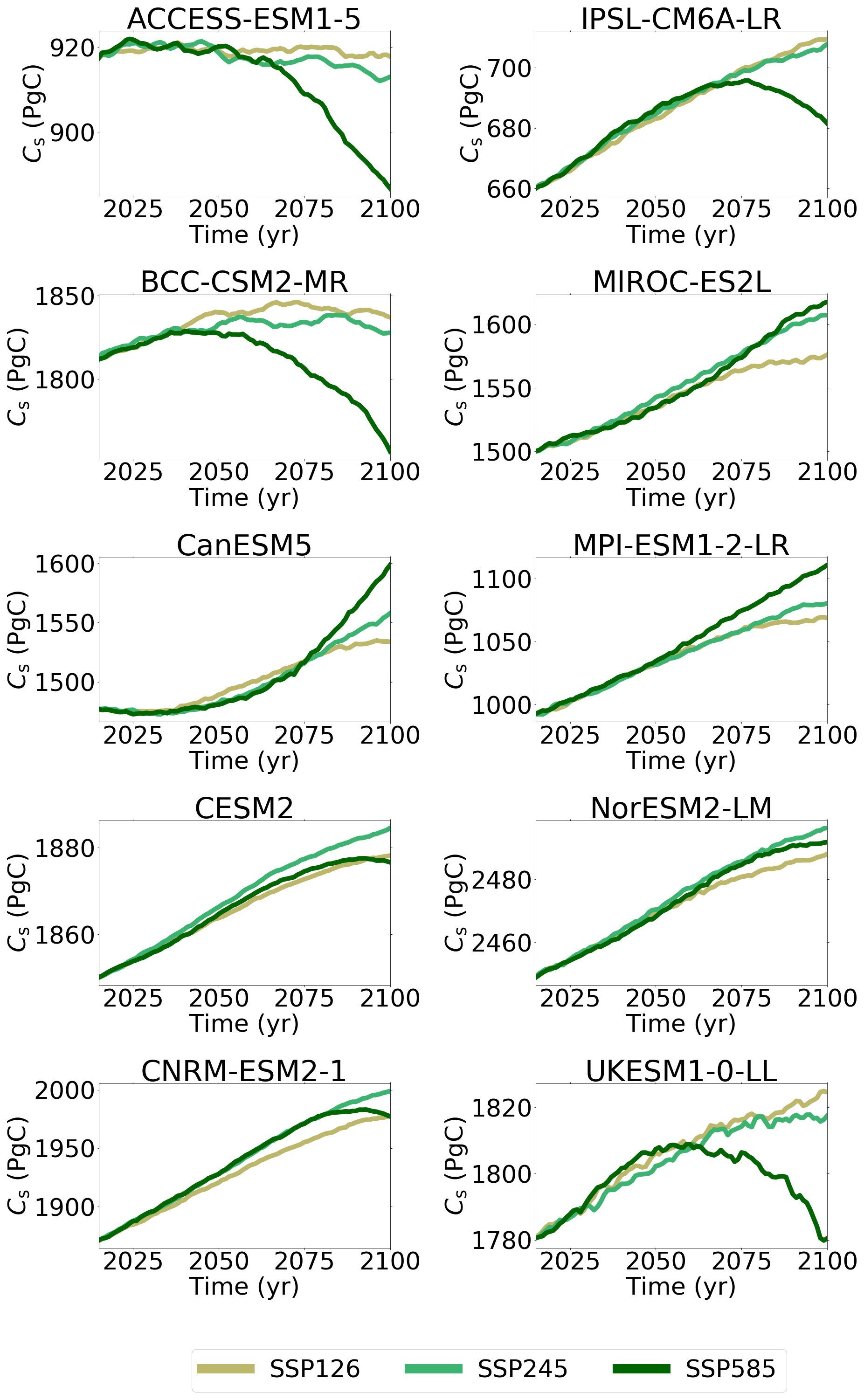
Figure 2 Time series of projected future soil carbon (C_s) in CMIP6 ESMs for future climate scenarios SSP126, SSP245, and SSP585.

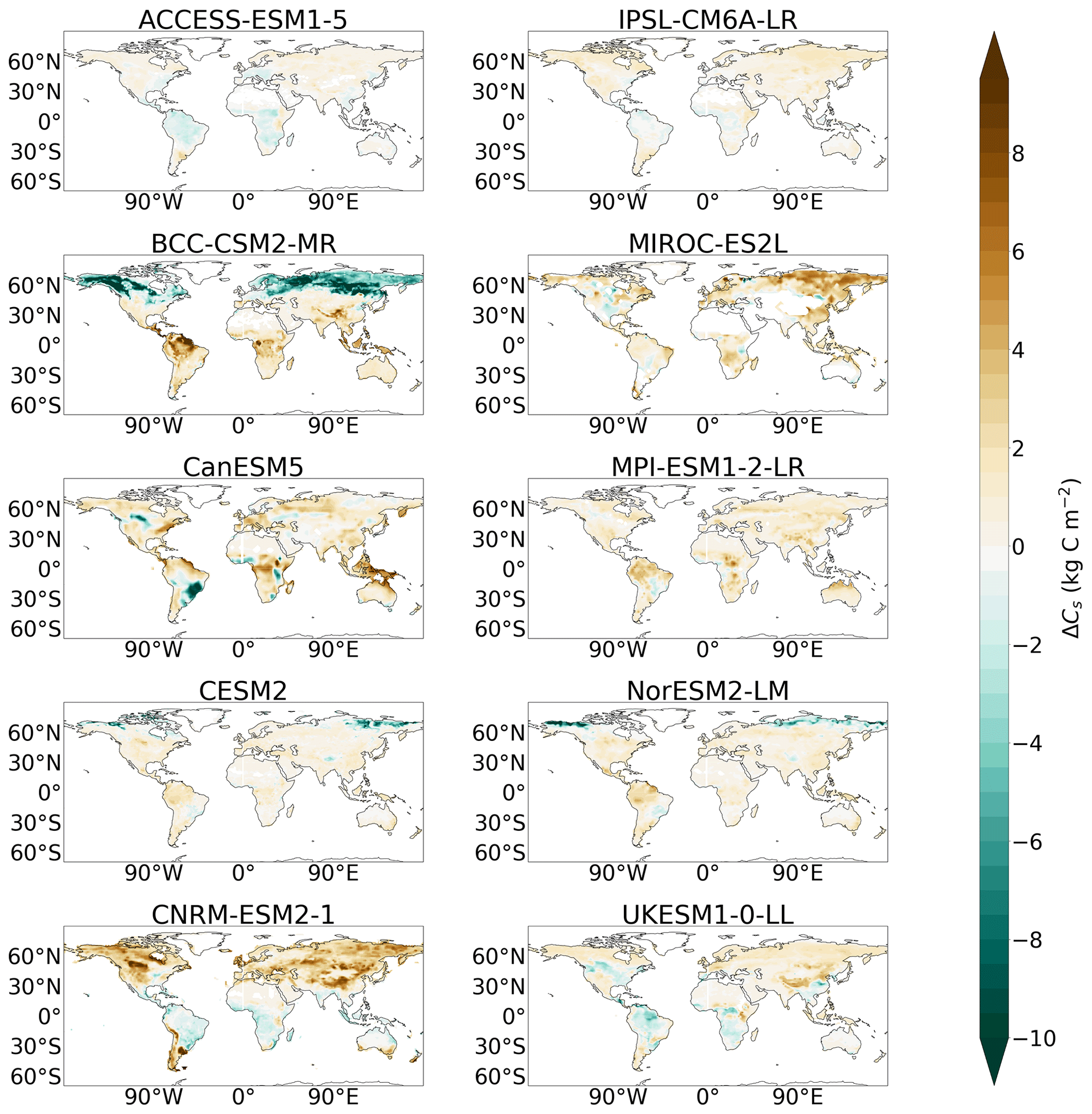
Figure 3 Map plots showing the change in soil carbon (ΔC_s) in SSP585 for each CMIP6 ESM.

The spatial pattern of estimated ΔC_s (Fig. 3) is quite variable between CMIP6 ESMs in the tropical regions, where increases in soil carbon can be seen in six of the CMIP6 ESMs (BCC-CSM2-MR, CanESM5, CESM2, MIROC-ES2L, and NorESM2-LM) but decreases are seen in the remaining four (ACCESS-ESM1-5, CNRM-ESM2-1, IPSL-CM6A-LR, and UKESM1-0-LL). There is a lack of agreement in the high northern latitudes amongst the CMIP6 ESMs (Fig. 3), where it is known that the uncertainty surrounding the fate of soil carbon stocks in these regions is particularly important due to the large magnitude of carbon stored (Burke et al., 2020; Jackson et al., 2017). It has previously been found that a high accumulation of northern-latitude C_s is predicted amongst CMIP5 ESMs; however, this C_s response has not been suggested in empirical studies based on observational findings (Todd-Brown et al., 2014). The results here suggest that this accumulation (increased ΔC_s) remains in the majority of CMIP6 ESMs (Fig. 3), although reductions in northern-latitude soil carbon stocks were found in three CMIP6 ESMs (BCC-CSM2-MR, CESM2, and NorESM2-LM, with BCC-CSM2-MR seeing reductions in a greater area). These ESMs which predicted northern-latitude C_s reductions were previously found to simulate historical northern-latitude soil carbon stocks which are more consistent with the observational estimates seen in these regions (Varney et al., 2022).

3.2 Future changes to land–atmosphere fluxes

The projected ΔC_s is a result of the changing input and output land–atmosphere fluxes under climate change. To a first order, the response of soil carbon will be determined by changes to NPP and to τ_s (see Eq. 7). In this section, future projections of these fluxes are analysed in both CMIP6 and CMIP5 ESMs.

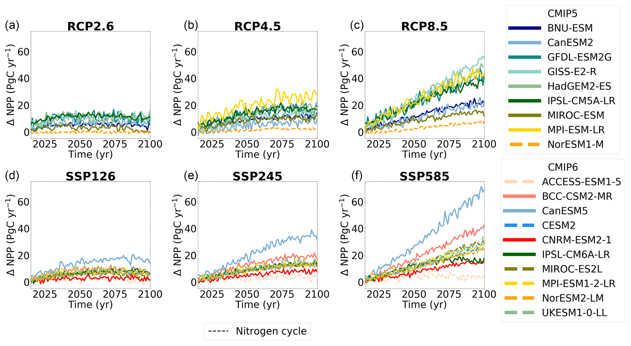
Figure 4 Projected future change in net primary productivity (ΔNPP) in CMIP5 (a–c) and CMIP6 (d–f) ESMs for future climate scenarios RCP2.6 and SSP126, RCP4.5 and SSP245, and RCP8.5 and SSP585, respectively. The dashed lines represent ESMs which include the representation of interactive nitrogen in these simulations.

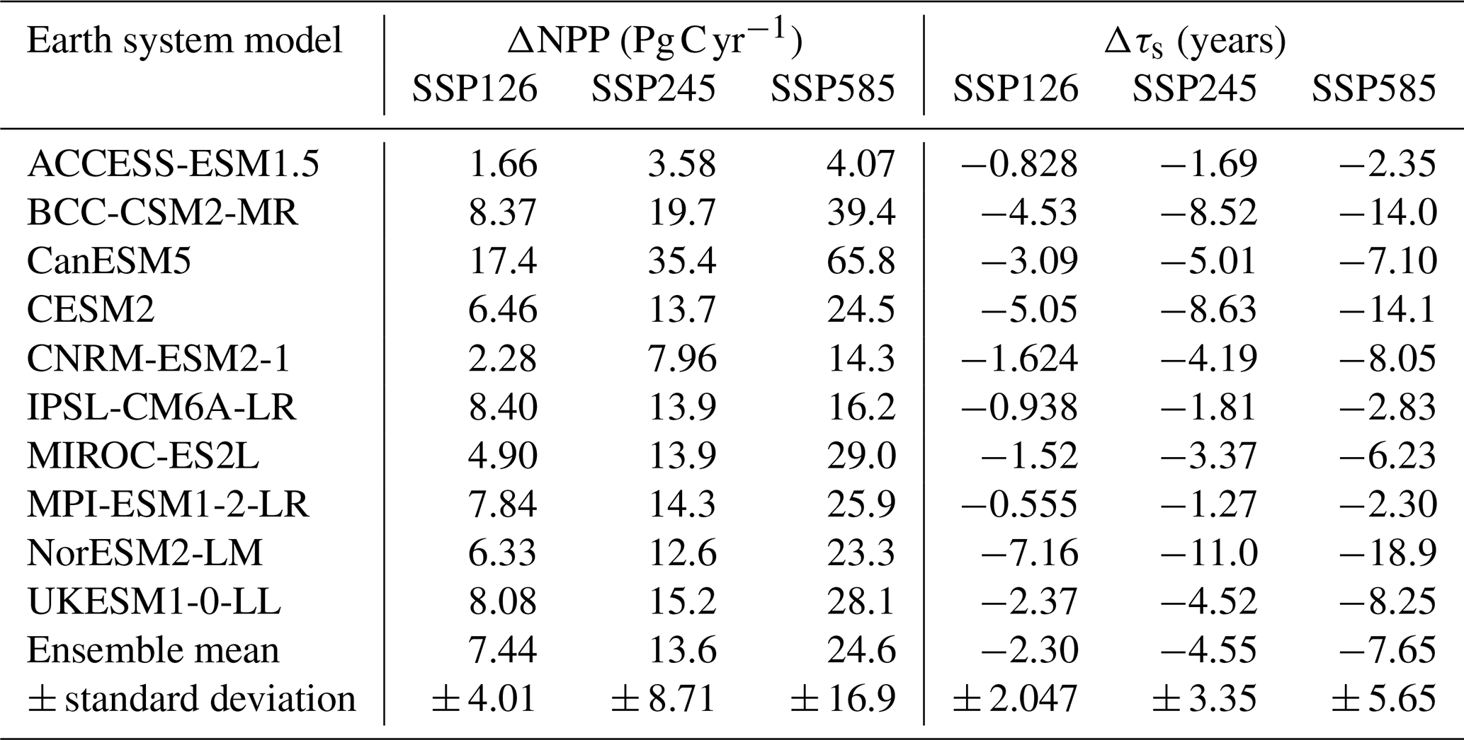
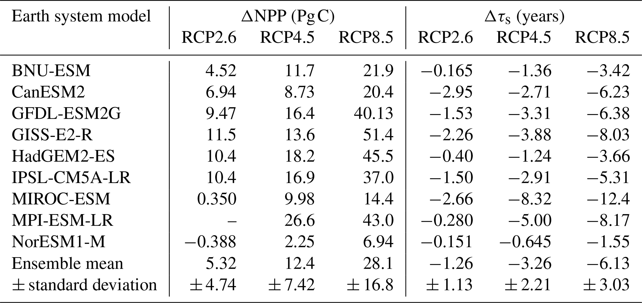
Table 3 Table presenting the change in 21st century NPP and τ_s for each CMIP6 model as well as the ensemble mean ± standard deviation, for each future SSP scenario.

3.2.1 Net primary productivity

NPP is projected by CMIP6 ESMs to increase during the 21st century, with a greater increase with increasing climate forcing (across SSP scenarios). This result is consistent with the projections of ΔNPP amongst the CMIP5 models (Fig. 4; Todd-Brown et al., 2014). Projections amongst ESMs, however, show disagreement in the magnitude of ΔNPP by 2100 across all future climate scenarios, where a projected CMIP6 ensemble increase of 24.6 ± 16.9 Pg C yr⁻¹ is seen in SSP585. The largest projections of ΔNPP amongst the CMIP6 models are seen in CanESM5 and BCC-CSM2-MR, where increases of 65.8 Pg C yr⁻¹ (47 % increase) and 39.4 Pg C yr⁻¹ (43 % increase), respectively, are projected by 2100 under SSP585. This is compared to ACCESS-ESM1-5, which has the lowest projected changes amongst the CMIP6 models, with an increase of only 4.07 Pg C yr⁻¹ (10 % increase) by 2100 under SSP585 (Table 3).

The CMIP6 ensemble sees a slightly increased range in end-of-century ΔNPP compared with CMIP5 across all future scenarios (Tables 3 and A2). Figure 4 suggests that the increased range is mostly due to outlying projections of ΔNPP (CanESM5), where greater increases are seen compared to the majority of models within the ensemble. It is noted that a cluster of ESMs which have similar projections of ΔNPP is seen within CMIP6 (CESM2, MIROC-ES2L, MPI-ESM1-2-LR, NorESM2-LM, and UKESM1-0-LL). The cluster is found to be made up of ESMs which include the simulation of an interactive nitrogen cycle (shown by the dashed lines throughout this study), which is a common addition within CMIP6 ESMs (ACCESS-ESM1.5, CESM2, MIROC-ES2L, MPI-ESM1-2-LR, NorESM2-LM, and UKESM1-0-LL; Davies-Barnard et al., 2020). ACCESS-ESM1-5 is the only model within CMIP6 which simulates interactive nitrogen, but it does not predict a similar ΔNPP to the other nitrogen ESMs in CMIP6. However, the projections of ΔNPP in ACCESS-ESM1-5 are similar to the projections of NorESM1-M in CMIP5, which is the only CMIP5 model considered here to simulate interactive nitrogen (Table 1).

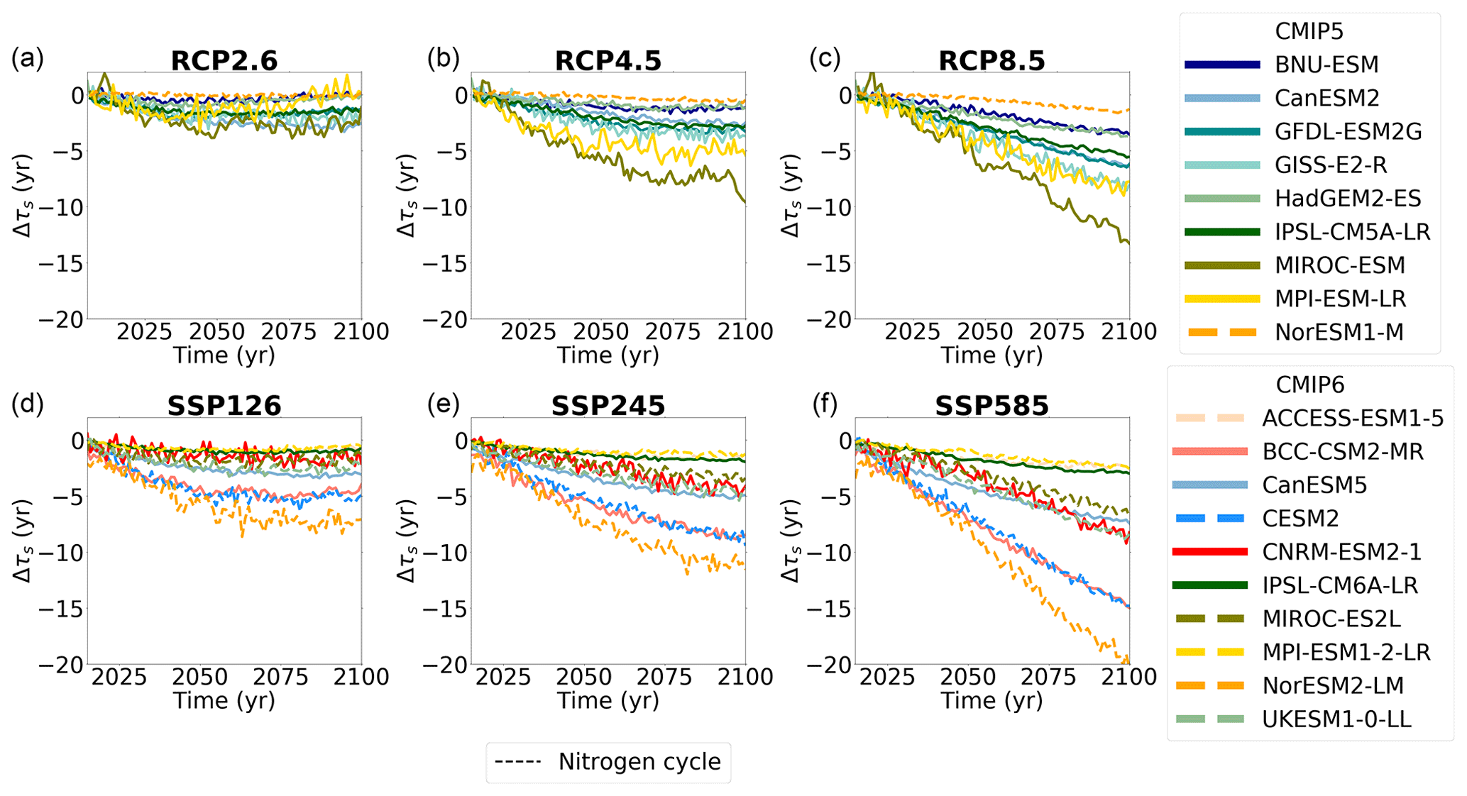
Figure 5 Projected future change in soil carbon turnover time (Δτ_s) in CMIP5 (a–c) and CMIP6 (d–f) ESMs for future climate scenarios RCP2.6 and SSP126, RCP4.5 and SSP245, and RCP8.5 and SSP585, respectively. The dashed lines represent ESMs which include the representation of interactive nitrogen in these simulations.

3.2.2 Soil carbon turnover time

Future τ_s is projected by CMIP6 ESMs to decrease by 2100 across all future SSP scenarios (Fig. 5). A greater reduction in τ_s is seen with the increased climate forcing scenario, where a reduced τ_s is a faster soil carbon turnover time and implies that carbon is cycled back to the atmosphere in less time due to an increased carbon output from the soil (increased R_h; see Eq. 1). This result is consistent with the projections of Δτ_s amongst the CMIP5 models (Fig. 5; Todd-Brown et al., 2014). However, it is found that greater variation exists amongst the CMIP6 ESMs' end-of-century estimates, where a projected CMIP6 ensemble Δτ_s value of −7.65 ± 5.65 years is seen in SSP585 compared to −6.13 ± 3.03 years for CMIP5 ESMs in RCP8.5 (Tables 3 and A2).

The CMIP6 ESMs with the greatest reductions in effective global τ_s by 2100 are seen in BCC-CSM2-MR, CESM2, and NorESM2-LM, where global carbon turnover in the soil is at least 14 years faster at the end of the SSP585 simulation compared to the start of the 21st century (historical reference). The CMIP6 models with the least change in effective global τ_s are ACCESS-ESM1-5, IPSL-CM6A-LR, and MPI-ESM1-2-LR, where global carbon turnover in the soil is only around 2 years faster at the end of the SSP585 simulation (Table 3). The increased range in CMIP6 from CMIP5 is primarily due to the large τ_s reductions seen in the CMIP6 models NorESM2-LM, CESM2, and BCC-CSM2-MR (Fig. 5).

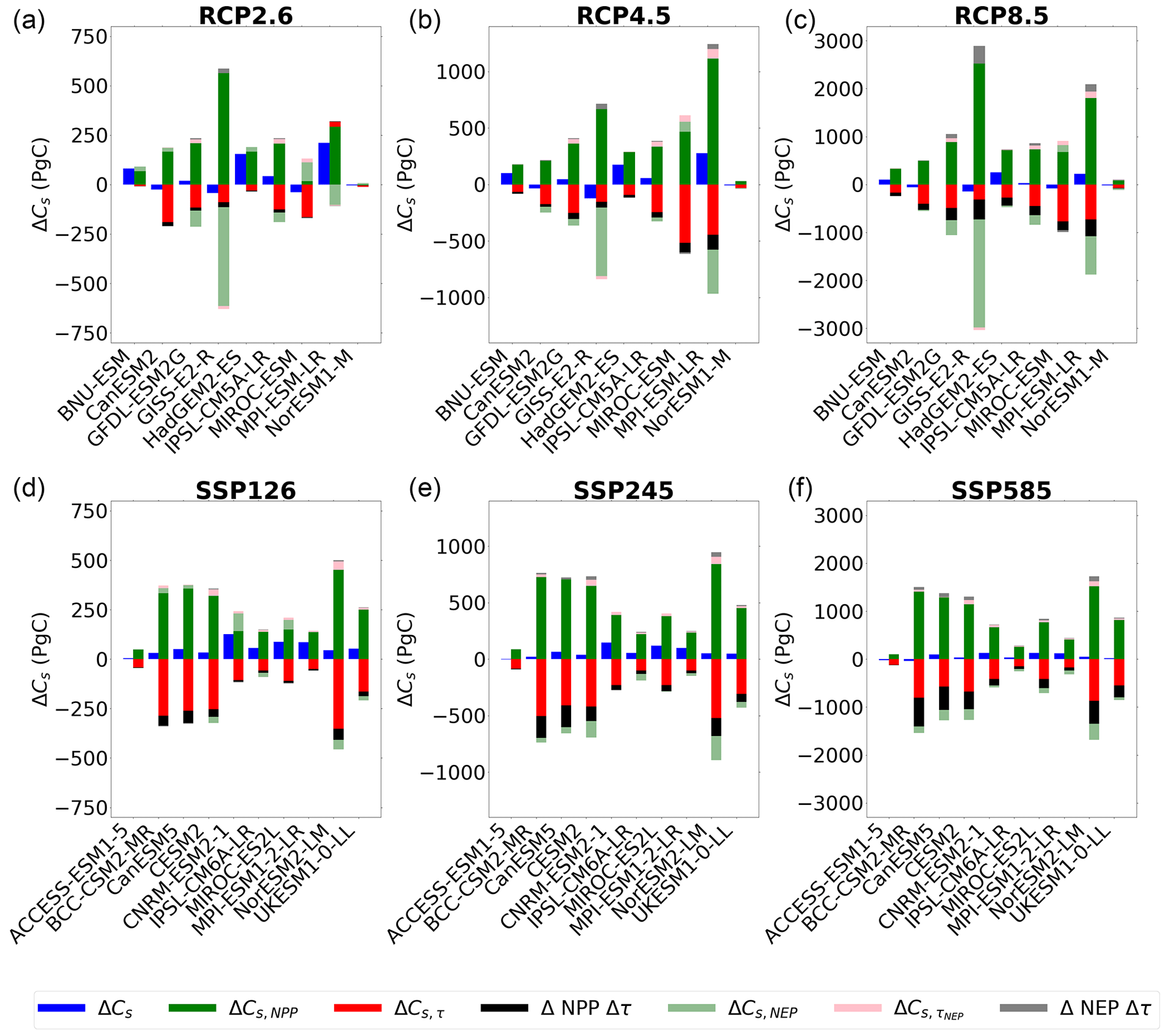
Figure 6 A bar chart showing the contributions of NPP and τ_s to end-of-21st-century changes in soil carbon (ΔC_s) in CMIP5 (a–c) and CMIP6 (d–f) ESMs for future scenarios RCP2.6 and SSP126, RCP4.5 and SSP245, and RCP8.5 and SSP585, respectively. The included terms are the linear term representing changes in soil carbon due to the changes in NPP (ΔC_s,NPP), the linear term representing changes in soil carbon due to the changes in τ_s (ΔC_s,τ), the non-linear term (ΔNPPΔτ_s), and then additional terms to account for the non-equilibrium climate in 2100 (ΔC_s,NEP, $\mathrm{\Delta }{\mathrm{C}}_{\mathrm{s},{\mathit{\tau }}_{\mathrm{NEP}}}$, and ΔNEPΔτ_s).

3.3 Breaking down the projected changes in soil carbon

To understand the projected end-of-century changes in soil carbon storage (ΔC_s) in ESMs, the individual responses of soil carbon due to changes in NPP (ΔC_s,NPP; see Eq. 9) and the response due to changes in τ_s (ΔC_s,τ; see Eq. 11) were diagnosed for both CMIP5 and CMIP6 as shown in Fig. 6. Future ΔC_s (blue bars) is found to be mostly a result of the net effect of the linear terms ΔC_s,NPP (dark-green bars) and ΔC_s,τ (red bars). However, there are also non-negligible contributions from the non-linear term ΔNPPΔτ_s (black bars) and a small addition due to the non-equilibrium terms ΔC_s,NEP (light-green bars), $\mathrm{\Delta }{\mathrm{C}}_{\mathrm{s},{\mathit{\tau }}_{\mathrm{NEP}}}$ (pink bars), and ΔNEPΔτ_s (grey bars).

The importance of investigating the individual processes which contribute to the net ΔC_s in ESMs can be seen (Fig. 6). In Fig. 6 it is seen that the net ΔC_s is relatively small compared to the individual changes from the derived components, where especially large magnitudes are seen in the increased C_s due to increased ΔNPP (ΔC_s,NPP) and the decreased C_s due to reduced Δτ_s (ΔC_s,τ). For example, in SSP585 there is a range of approximately 170 Pg C in net ΔC_s, from an increase of 132 Pg C (CNRM-ESM2-1) to a reduction of 35 Pg C (BCC-CSM2-MR). However, the ΔC_s,NPP contribution has a much larger range of 1442 Pg C, from an increase of 95 Pg C (ACCESS-ESM1-5) to an increase of 1517 Pg C (NorESM2-LM). Similarly, ΔC_s,τ has a range of 756 Pg C, from a decrease of 115 Pg C (ACCESS-ESM1-5) to a decrease of 871 Pg C (NorESM2-LM).

The magnitude of change seen from the individual feedbacks (ΔC_s,NPP and ΔC_s,τ) is not obviously related to the resultant magnitude of soil carbon change (Fig. A1). For example, NorESM2-LM projects large ΔC_s,NPP and ΔC_s,τ values (1517 and −871 Pg C in SSP585, respectively) but a relatively small net change in soil carbon (49 Pg C in SSP585). Conversely, CNRM-ESM2-1 projects smaller ΔC_s,NPP and ΔC_s,τ values (667 and −413 Pg C in SSP585, respectively) but a larger net soil carbon change (132 Pg C in SSP585). Within ESMs, it is found that the change in soil carbon is determined by the relationship between all the contributing terms to the net ΔC_s response, as opposed to the absolute size of a given contribution (Fig. 6).

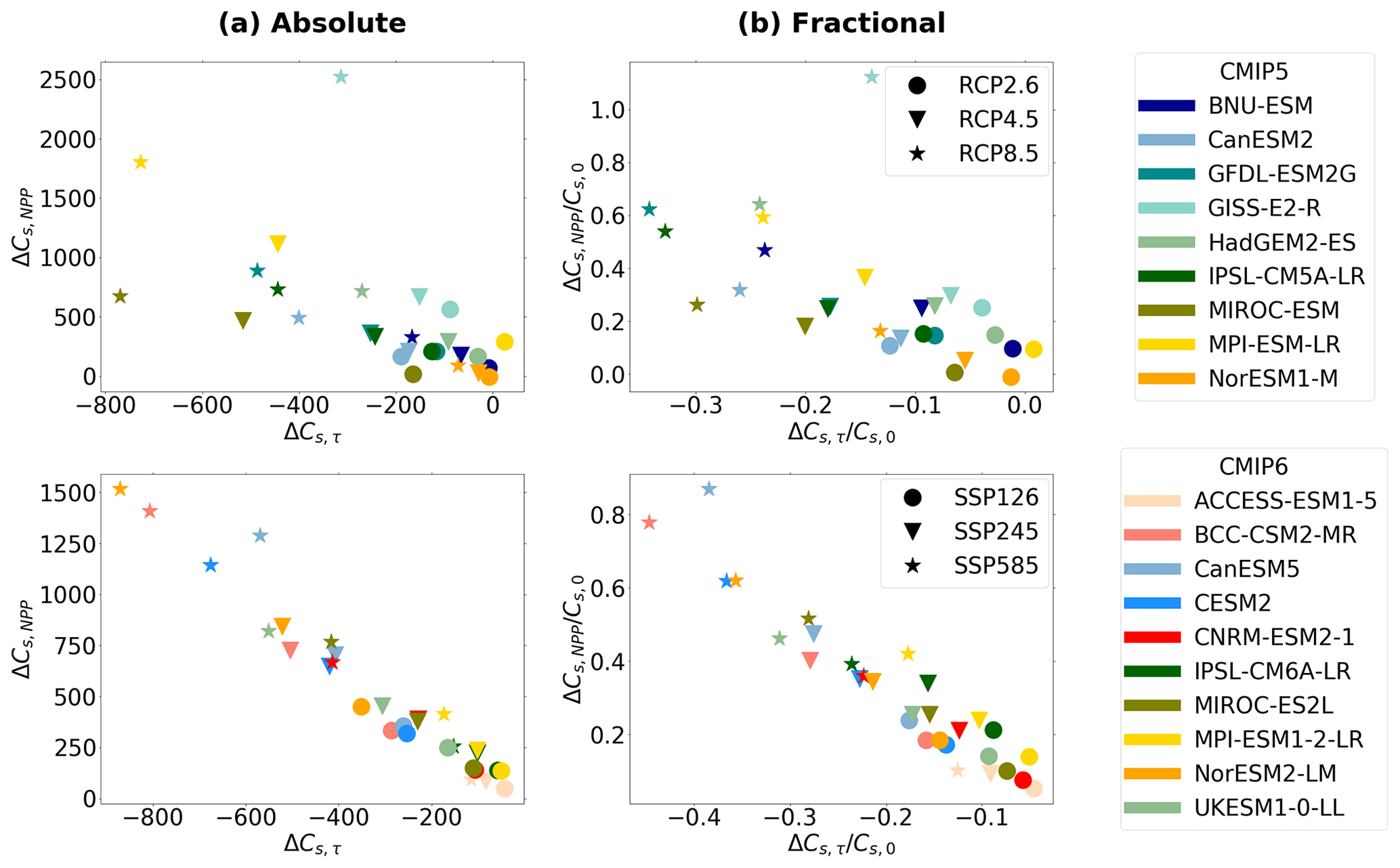
Figure 7 Scatter plot comparing the relationship between ΔC_s,NPP and ΔC_s,τ for CMIP5 (top row) and CMIP6 (bottom row) ESMs in future scenarios RCP2.6 and SSP126, RCP4.5 and SSP245, and RCP8.5 and SSP585, respectively, for (a) absolute changes and (b) fractional changes.

Surprisingly, a very strong correlation is found amongst the ESMs in CMIP6 (r² value of 0.97) between the linear terms ΔC_s,NPP and ΔC_s,τ (Fig. 7a). This leads to the partial cancelling of the terms, with a relatively small resultant net ΔC_s. When comparing with the CMIP5 ensemble, a lower correlation between ΔC_s,NPP and ΔC_s,τ is seen (r² value of 0.084, Fig. 7a). This correlation amongst CMIP6 ESMs results in net ΔC_s being more clustered in CMIP6 compared to CMIP5 (Fig. 1) despite a similarly large variation in the individual contributions (Fig. 6). The strong CMIP6 correlation (r²=0.97) remains when the fractional changes ($\mathrm{\Delta }{\mathrm{C}}_{\mathrm{s},\mathrm{NPP}}/{\mathrm{C}}_{\mathrm{s},\mathrm{0}}$ and $\mathrm{\Delta }{\mathrm{C}}_{\mathrm{s},{\mathit{\tau }}_{\mathrm{NPP}}}/{\mathrm{C}}_{\mathrm{s},\mathrm{0}}$, where C_s,0 is initial soil carbon stocks) are plotted instead (Fig. 7b).

Figure 6 also shows that the differences in ESM projections of ΔC_s are partly due to differing magnitudes of the non-linear term (ΔNPPΔτ_s). A linear assumption is commonly used which would allow these cross-terms to be neglected ($\mathrm{\Delta }\mathrm{NPP}/\mathrm{NPP}\ll \mathrm{1}$ and $\mathrm{\Delta }{\mathit{\tau }}_{\mathrm{s}}/{\mathit{\tau }}_{\mathrm{s}}\ll \mathrm{1}$; Koven et al., 2015). However, the ESM-projected magnitudes of ΔNPPΔτ_s are found to be relatively large, especially in the more extreme climate scenarios (Fig. 6). In SSP585, a range from a decreased C_s of 11 Pg C (ACCESS-ESM1-5) to a decreased C_s of 599 Pg C (BCC-CSM2-MR) is found amongst the CMIP6 models due to only the ΔNPPΔτ_s term, and in some cases values greater magnitudes are seen than the net ΔC_s (BCC-CSM2-MR, CanESM5, CESM2, NorESM2-LM, and UKESM1-0-LL). The term is greater when there are large and counteracting magnitudes of ΔNPP and Δτ_s, which results in a non-negligible product.

Additionally, to obtain the overall change in soil carbon seen in the models, contributions from the non-equilibrium terms (ΔC_s,NEP, $\mathrm{\Delta }{\mathrm{C}}_{\mathrm{s},{\mathit{\tau }}_{\mathrm{NEP}}}$, and ΔNEPΔτ_s) must also be included (Fig. 6). The ΔC_s,NEP term represents the change in soil carbon due to the net carbon sink during the 21st century, which exists while the climate is in a transient state due to continuous climate change. By definition, the magnitude of ΔC_s,NEP is negative if ΔNEP is positive, which implies a greater or faster increase in NPP with respect to R_h seen in the majority of ESMs. The contribution from these terms is found to be relatively small in most models but not in all. In SSP585, projections of ΔC_s,NEP amongst the CMIP6 models range from a reduction of 333 Pg C (NorESM2-LM) to a gain of 8.74 Pg C (ACCESS-ESM1-5). In CMIP5, there are exceptions where greater ΔC_s,NEP terms are found in the GISS-E2-R and MPI-ESM-LR models, implying that the models are far from equilibrium at the end of the 21st century. The change in soil carbon due to the change in NEP (ΔC_s,NEP) is often found to be greater in the models, which see greater magnitudes of ΔC_s,NPP and ΔC_s,τ.

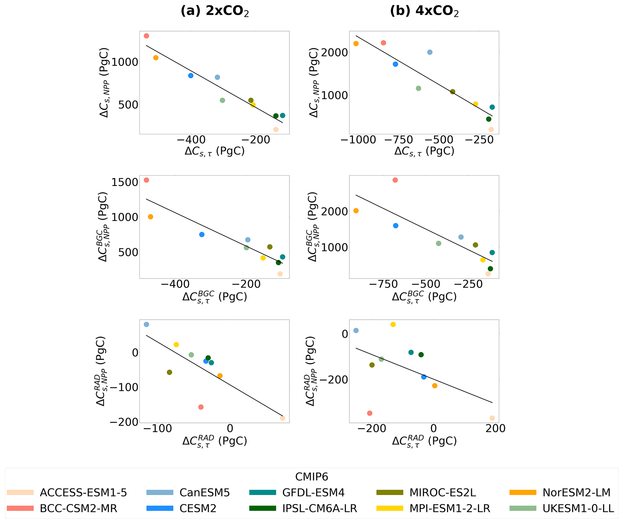
Figure 8 Scatter plots showing the relationship between ΔC_s,NPP and ΔC_s,τ for each CMIP6 ESM in the full 1 % CO₂ simulation (top row), BGC simulation (middle row), and RAD simulation (bottom row) for (a) 2 × CO₂ and (b) 4 × CO₂.

3.4 Investigating the emergent relationship between ΔC_s,NPP and ΔC_s,τ

In this sub-section, the emergent relationship between ΔC_s,NPP and ΔC_s,τ present across the CMIP6 ensemble is investigated using the idealised C4MIP simulations (see Methods). This enables investigation of the apparent negative correlation without additional complex processes which are included in the SSP simulations. By isolating the sensitivities to CO₂ and climate, we can more easily identify the processes, which results in the apparent coupling between NPP and soil carbon turnover time in CMIP6 ESMs. Figure 8 presents the relationship between ΔC_s,NPP and ΔC_s,τ for each CMIP6 ESM as in Fig. 7 but for the full 1 % CO₂, BGC (CO₂ only), and RAD (climate only) simulations. It is found that ΔC_s,NPP and ΔC_s,τ are strongly correlated in the full 1 % CO₂ simulation at both 2 × CO₂ (r² value of 0.925) and 4 × CO₂ (r² value of 0.839). The correlation is found to remain in the BGC simulation, where r² values are found to be 0.838 and 0.708 for 2 × CO₂ and 4 × CO₂, respectively. A correlation is also seen in the RAD simulation at 2 × CO₂ (r² value of 0.601); however, the correlation in the RAD simulation does not hold at 4 × CO₂, where the r² value reduces to 0.265. The reduced correlation in the RAD simulation at 4 × CO₂ suggests a reduced relationship between NPP and τ_s at the more extreme temperature changes that are projected at high levels of atmospheric CO₂ (without the direct effects of CO₂ in this run).

For each CMIP6 ESM, NPP and τ_s are found to be strongly inversely correlated in the full 1 % CO₂ simulation (Fig. 9). The r² values between $\mathrm{NPP}/{\mathrm{NPP}}_{\mathrm{0}}$ and ${\mathit{\tau }}_{\mathrm{s},\mathrm{0}}/{\mathit{\tau }}_{\mathrm{s}}$ (where the subscript 0 denotes the historical state) are found to be greater than 0.95 in all the models, except for ACCESS-ESM1-5 (where an r² value of 0.65 is found due to a breakdown at high CO₂ levels). In the BGC simulation, a similar relationship between $\mathrm{NPP}/{\mathrm{NPP}}_{\mathrm{0}}$ and ${\mathit{\tau }}_{\mathrm{s},\mathrm{0}}/{\mathit{\tau }}_{\mathrm{s}}$ is seen up until approximately 2 × CO₂ in all the ESMs (approximately 50 % of the simulation). However, how the relationship between $\mathrm{NPP}/{\mathrm{NPP}}_{\mathrm{0}}$ and ${\mathit{\tau }}_{\mathrm{s},\mathrm{0}}/{\mathit{\tau }}_{\mathrm{s}}$ changes throughout the BGC simulation (between 2 × CO₂ and 4 × CO₂) varies between the models. A greater rate of $\mathrm{NPP}/{\mathrm{NPP}}_{\mathrm{0}}$ increase compared to ${\mathit{\tau }}_{\mathrm{s},\mathrm{0}}/{\mathit{\tau }}_{\mathrm{s}}$ is seen at greater levels of climate forcing for the majority of CMIP6 ESMs (BCC-CSM2-MR, CanESM5, GFDL-ESM4, IPSL-CM6A-LR, MIROC-ES2L, MPI-ESM1-2-LR, and UKESM1-0-LL), where the τ_s changes appear to saturate and a limit to the increase is seen. In these ESMs, the changes seen in the full and BGC simulations differ due to a climate effect (shown by the RAD simulation), which appears to negate the apparent limit or saturation seen in the ${\mathit{\tau }}_{\mathrm{s},\mathrm{0}}/{\mathit{\tau }}_{\mathrm{s}}$ increase in the BGC simulation (Fig. 9). In CESM2 and NorESM2-LM (containing the same land surface model component), a consistent relationship is seen in both the full 1 % CO₂ and BGC simulations, suggesting that the changes in NPP and τ_s are primarily driven by changes in CO₂ concentrations or that the climate affects cancel out to a resultant net zero change. In ACCESS-ESM1-5, a consistent relationship is seen in the full 1 % CO₂, BGC, and RAD simulations, suggesting a greater sensitivity of NPP to environmental climate changes compared to the other CMIP6 ESMs (Fig. 9).

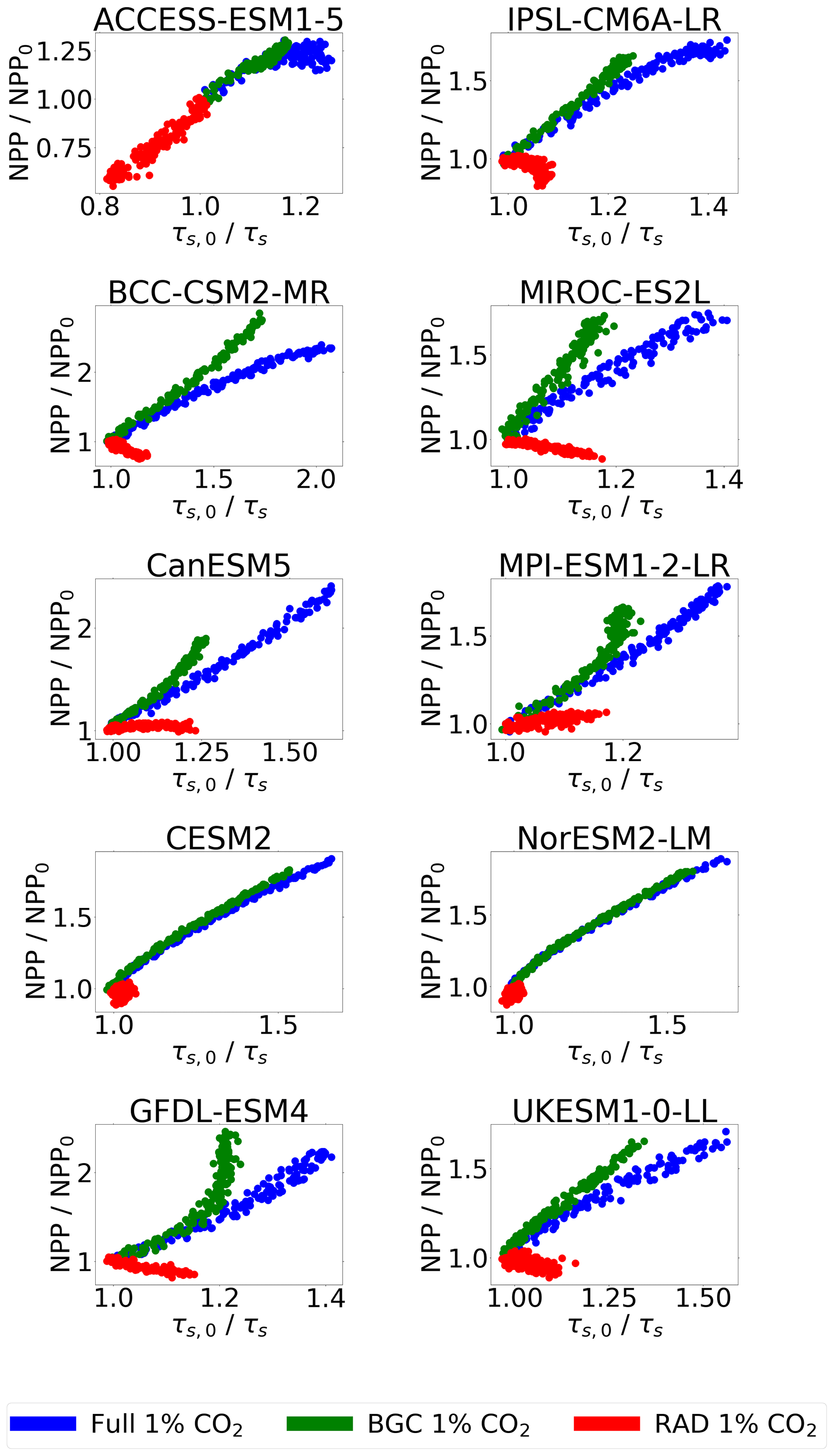
Figure 9 Scatter plots showing the correlation between $\mathrm{NPP}/{\mathrm{NPP}}_{\mathrm{0}}$ and ${\mathit{\tau }}_{s,\mathrm{0}}/{\mathit{\tau }}_{\mathrm{s}}$ for each CMIP6 ESM in the full 1 % CO₂ simulation (blue) and the BGC simulation (green) up to 4 × CO₂.

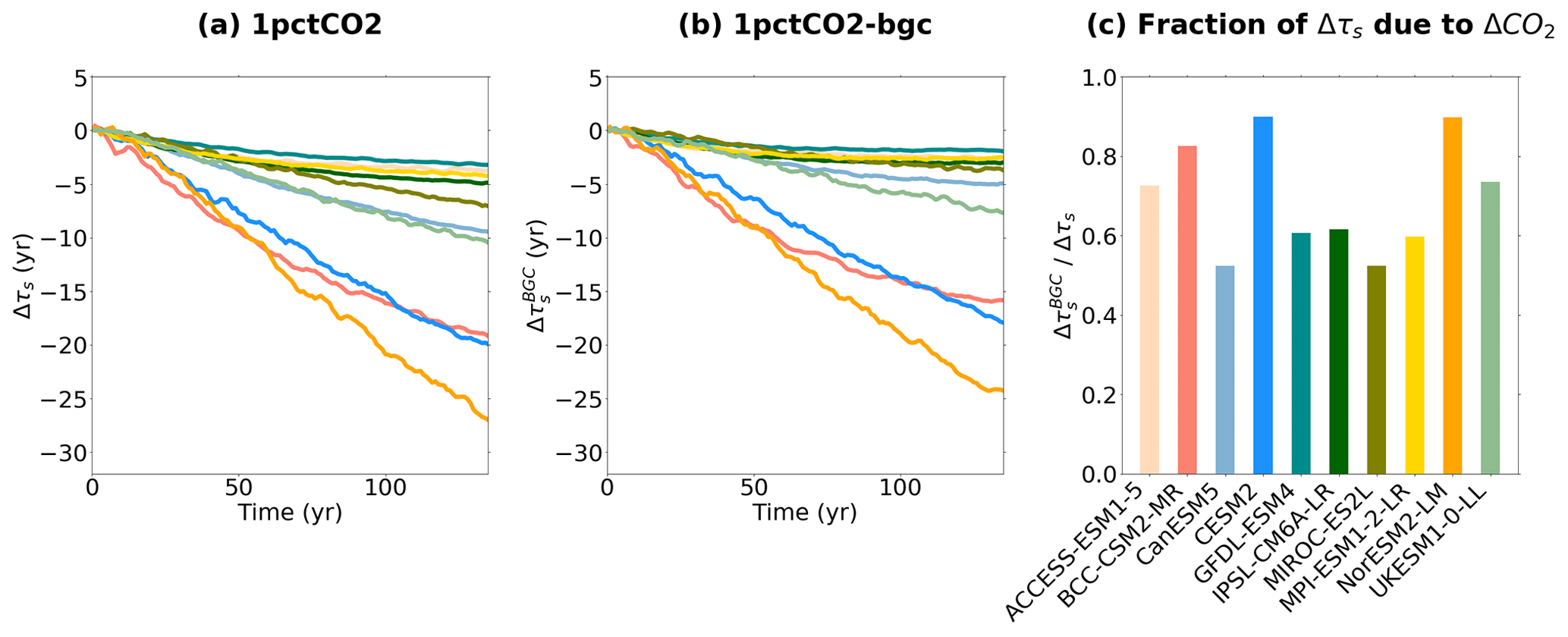
Figure 10 Changes in soil carbon turnover (Δτ_s) in C4MIP runs for the CMIP6 ESMs, with and without direct climate effects on τ_s. (a) Time series of Δτ_s in the full 1 % CO₂ simulation (climate and CO₂ changes), (b) time series of Δτ_s in the BGC simulation (CO₂ changes only), and (c) bar chart showing the fraction of total Δτ_s due to the changes in CO₂ at 4 × CO₂ for each model.

It has been shown in this sub-section that the correlation between ΔC_s,NPP and ΔC_s,τ, as seen in the SSP simulations (Fig. 7), is also evident in the full 1 % CO₂ C4MIP simulation (Fig. 8). This suggests that the relationship is not a result of additional processes included in the SSP simulations compared to the C4MIP experiments, such as land use change (Jones et al., 2016). An additional explanation for the coupling could be similarities in the modelled sensitivities of NPP and R_h to changes in climate (i.e. temperature and moisture changes). For example, if NPP and soil respiration rate both increased with warming, a negative correlation between ΔC_s,NPP and ΔC_s,τ would be seen. However, under these circumstances, the negative correlation would not be seen in the CO₂-only runs (BGC simulation), as there is no global warming in these simulations (see Methods). Instead, a reduction in the effective soil carbon turnover time is seen in the CO₂-only runs (BGC simulation; Fig. A2), which implies a non-climate response in τ_s and results in a NPP–τ_s negative correlation under changing atmospheric CO₂ alone (Fig. 9). Figure 10 shows that the change in the effective soil carbon turnover time in the CO₂-only simulation (BGC simulation) accounts for at least 50 % of the total change in the effective soil carbon turnover time in the full 1 % simulation across CMIP6 ESMs.

3.5 The role of false priming

Koven et al. (2015) present the concept of false priming as a reduction in effective soil carbon turnover time (τ_s) due to increases in productivity (NPP). It was defined as “false priming” due to the impact being similar to the “true priming” process, but it occurs without simulating the priming mechanisms, where priming is defined as the stimulation of decomposition of soil carbon (reducing τ_s) due to input of carbon to the soil (Liu et al., 2020). The false priming reduction in effective τ_s is a transient phenomenon that arises in soil models that represent multiple carbon pools with different turnover times. Under continually increasing NPP, proportionally more of the additional input litter carbon is put into the faster soil carbon pools than the slow ones, which brings down the global average effective τ_s value of the soil. In this sub-section, false priming is explored as a possible explanation for the negative correlation seen between NPP and τ_s, which are seen even in the BGC simulations (CO₂ only), where the climate does not change significantly (Fig. 10).

Koven et al. (2015) demonstrate false priming with a simple three-box soil carbon model, which has been adapted here to use notation consistent with the rest of this study:

$$\begin{array}{}\text{(13)}& {\displaystyle \frac{\mathrm{d}{\mathrm{C}}_{\mathrm{s},\mathrm{1}}}{\mathrm{d}t}}=\mathrm{NPP}-{\displaystyle \frac{{\mathrm{C}}_{\mathrm{s},\mathrm{1}}}{{\mathit{\tau }}_{\mathrm{s},\mathrm{1}}}},\text{(14)}& {\displaystyle \frac{\mathrm{d}{\mathrm{C}}_{\mathrm{s},\mathrm{2}}}{\mathrm{d}t}}={\displaystyle \frac{e_{\mathrm{1}}{\mathrm{C}}_{\mathrm{s},\mathrm{1}}}{{\mathit{\tau }}_{\mathrm{s},\mathrm{1}}}}-{\displaystyle \frac{{\mathrm{C}}_{\mathrm{s},\mathrm{2}}}{{\mathit{\tau }}_{\mathrm{s},\mathrm{2}}}},\text{(15)}& {\displaystyle \frac{\mathrm{d}{\mathrm{C}}_{\mathrm{s},\mathrm{3}}}{\mathrm{d}t}}={\displaystyle \frac{e_{\mathrm{2}}{\mathrm{C}}_{\mathrm{s},\mathrm{2}}}{{\mathit{\tau }}_{\mathrm{s},\mathrm{2}}}}-{\displaystyle \frac{{\mathrm{C}}_{\mathrm{s},\mathrm{3}}}{{\mathit{\tau }}_{\mathrm{s},\mathrm{3}}}},\text{(16)}& {\displaystyle }{R}_{\mathrm{h}}={\displaystyle \frac{(\mathrm{1}-e_{\mathrm{1}}){\mathrm{C}}_{\mathrm{s},\mathrm{1}}}{{\mathit{\tau }}_{\mathrm{s},\mathrm{1}}}}+{\displaystyle \frac{(\mathrm{1}-e_{\mathrm{2}}){\mathrm{C}}_{\mathrm{s},\mathrm{2}}}{{\mathit{\tau }}_{\mathrm{s},\mathrm{2}}}}+{\displaystyle \frac{(\mathrm{1}-e_{\mathrm{3}}){\mathrm{C}}_{\mathrm{s},\mathrm{3}}}{{\mathit{\tau }}_{\mathrm{s},\mathrm{3}}}},\text{(17)}& {\displaystyle }{\mathrm{C}}_{\mathrm{s}}={\mathrm{C}}_{\mathrm{s},\mathrm{1}}+{\mathrm{C}}_{\mathrm{s},\mathrm{2}}+{\mathrm{C}}_{\mathrm{s},\mathrm{3}},\text{(18)}& {\displaystyle }{\mathit{\tau }}_{\mathrm{s},\mathrm{1}}=\mathrm{1},{\mathit{\tau }}_{\mathrm{s},\mathrm{2}}=\mathrm{10},{\mathit{\tau }}_{\mathrm{s},\mathrm{3}}=\mathrm{100},\text{(19)}& {\displaystyle }{e}_{\mathrm{1}}=\mathrm{0.3},e_{\mathrm{2}}=\mathrm{0.3},e_{\mathrm{3}}=\mathrm{0},\end{array}$$

where C_s,1, C_s,2, and C_s,3 represent the carbon stored in soil carbon pools 1, 2, and 3 and make up the total soil carbon (C_s). Similarly, τ_s,i are the respective soil carbon turnover times, which are given defined values of increasing turnover times in years: fast (1 year), medium (10 years), and slow (100 years). NPP represents the carbon input into the system, where carbon is inputted into pool 1 (C_s,1) and then flows to pools 2 (C_s,2) and 3 (C_s,3). The coefficient e_i represents the fraction of carbon that is passed to the next pool rather than outputted as heterotrophic respiration (R_h).

At equilibrium, the change in the soil carbon pools will be zero ($\mathrm{d}{\mathrm{C}}_{\mathrm{s},i}/\mathrm{d}t=\mathrm{0}$), so the amount of soil carbon present within each pool depends on the input carbon and turnover time of the pool (τ_s,i). Under increasing NPP, the three-box model can be used to investigate the subsequent changes to soil carbon in the three carbon pools (C_s,1, C_s,2, C_s,3) based on changing input alone, due to each pool having a fixed τ_s,i value. This removes the Δτ_s from changing environmental and microbial conditions (Koven et al., 2015; Wieder et al., 2015a; Exbrayat et al., 2013). The effective τ_s of the system is calculated by definition (using Eq. 1).

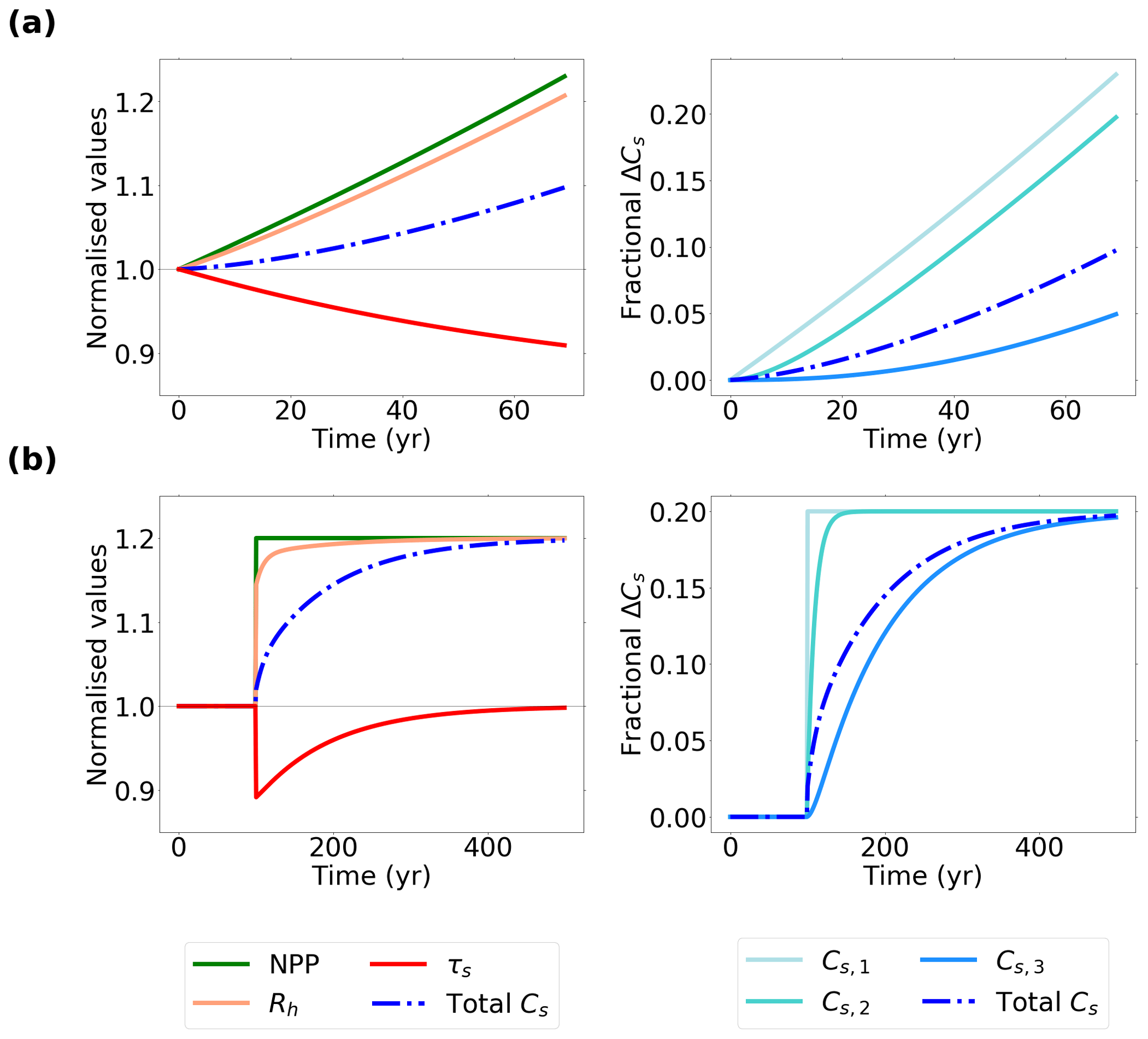
Figure 11 Time series plot showing the results from the simple three-box model. (a) For normalised changes in NPP, R_h, τ_s, and C_s as well as the fractional change in each of the three soil carbon boxes and in the total soil carbon (recreation of Fig. 12 in Koven et al., 2015). (b) For an abrupt change in global NPP from 50 to 70 Pg C yr⁻¹ at year 100.

Figure 11a shows a simulation of the response of this three-box model to an NPP input flux that increases at 0.3 % yr⁻¹ and where the soil carbon boxes are initialised at 0 (reproducing Fig. 12 in Koven et al., 2015). The greater fraction of ΔC_s in the fast soil carbon pool compared to the slow one can be seen, which results in a decline in the effective τ_s of the system. This decline in effective τ_s with increasing NPP is clear and demonstrates false priming (Fig. 11a). Figure 11b again demonstrates that false priming is a transient effect associated with the distribution of soil carbon between the three pools, which emerges from the differences in the mass-weighted and flux-weighted responses. It shows results from the same model but for a step increase in global NPP from 50 to 70 Pg C yr⁻¹ at year 100. The fast soil carbon pool reaches equilibrium before the slower soil carbon pool, resulting in the instantaneous decline in τ_s of about 10 %, which eventually reduces to return the soil to the original τ_s. This transient effect occurs on the timescale of the slowest carbon pool and therefore may take many centuries.

The same three-box model can also be used to investigate the relationship between the contributions of changes in NPP (ΔC_s,NPP) and τ_s (ΔC_s,τ) with net soil carbon change that was noted in both Figs. 7 and 8. Figure 12 plots ΔC_s,NPP against ΔC_s,τ from the three-box model after 70 years of runs that assume different rates of increase in NPP (0 % yr⁻¹ to 0.8 % yr⁻¹ in increments of 0.05 %). A clear relationship between ΔC_s,NPP and ΔC_s,τ is seen, with greater false priming (more negative ΔC_s,τ) when the NPP increase is larger (more positive ΔC_s,NPP). The similarity of Fig. 12 to both Figs. 7 and 8 is clear, suggesting that false priming and the structure of the soil carbon models within the ESMs are likely contributing to these correlations in CMIP6 (and to a lesser extent in CMIP5).

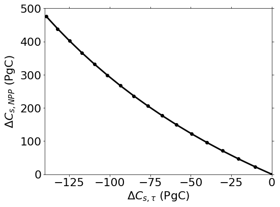
Figure 12 Relationship between ΔC_s,NPP and ΔC_s,τ derived from the three-box model. Each dot represents the results at the end of a 70-year run with a different assumed rate of increase in NPP (∼ 0.0 % yr⁻¹ to 0.8 % yr⁻¹ in increments of 0.05 %).

It is noted that the influence of false priming was stronger in the full 1 % CO₂ and BGC (CO₂ only) simulations compared to the RAD (climate only) simulation (Fig. 8). This is likely due to the RAD simulation not seeing sufficient NPP change and therefore sufficient input of soil carbon for the false priming effect to be significant (see Fig. A2). Additionally, the direct effect of temperature changes on τ_s in the RAD simulation (in the absence of atmospheric CO₂ changes) is likely to dampen the correlation with NPP changes, due to both direct and indirect Δτ_s influences in this case (Varney et al., 2020).

False priming refers to a reduction in the effective turnover time when the input of carbon into the soil increases. It was named “false priming” as it can look like the increase in heterotrophic respiration that occurs when a soil microbial community is stimulated by the addition of labile carbon or nutrients (“true priming”). However, false priming is arguably a misleading term because it is a real effect. It arises as a result of a change in the relative quantities of carbon turning over at different rates, which occurs transiently in response to an increase in the input of carbon into the soil. In the context of our three-box model, for example, the turnover rates of each individual box do not change. However, because each box responds differently to the increase in NPP, a difference in the average or effective turnover (i.e. as defined in Eq. 1) is seen. The effective soil carbon turnover time is a measure of how long carbon remains in the soil. However, it cannot necessarily be assumed that all carbon will take exactly the same amount of time to be re-released. Different types of litter input (e.g. lignin vs. carbohydrate) take different amounts of time to decompose (Krishna and Mohan, 2017). Similarly, vertical gradients in temperature throughout the soil result in variations of turnover time within the system (Koven et al., 2017). The effective carbon turnover time is an average of these distributions of turnover times, and an increase in the amount of fast turnover carbon in the system relative to slower turnover carbon results in it decreasing. As it has been shown here, this effect can be significant and must be accounted for when attributing soil carbon change to different environmental drivers (Georgiou et al., 2015).

This study has highlighted how false priming has contributed to a reduced spread in ΔC_s ESM projections in CMIP6, due to a cancellation effect seen between increases due to ΔNPP (ΔC_s,NPP) and decreases due to Δτ_s (ΔC_s,τ). The extent of false priming within ESM projections will depend on the distribution of carbon within soil carbon pools and how litter carbon is allocated between pools with fast and slow turnover times (Koven et al., 2015). Figure 10(c) shows the fraction of Δτ_s due to ΔCO₂, which can be used as a proxy to estimate the contribution of false priming to the overall projected Δτ_s in CMIP6 ESMs, which varies between approximately 50 % (CanESM5 and MIROC-ES2L) and 90 % (CESM2 and NorESM2-LM). A more apparent false priming affect within CMIP6 could suggest an improved representation of the slower components of soil carbon since CMIP5, commonly by including more dead carbon pools within the ESM (Table 1). Based on observational radiocarbon estimates, it has been found that CMIP5 ESMs underestimate carbon age within the soil (He et al., 2016; Shi et al., 2020), suggesting that ESMs underestimate the amount of carbon in the slow carbon pools. It has been shown that representing soil carbon ages more in line with radiocarbon estimates leads to a reduced potential for soil carbon sequestration in the future (He et al., 2016), which agrees qualitatively with the projected 21st century soil carbon changes as predicted by CMIP6 compared to CMIP5 found in this study.

On top of the role of false priming, additional factors influence the magnitude of predicted ΔC_s within ESMs. Generationally related ESMs between CMIP5 and CMIP6 allow us to highlight some key changes between the CMIP generations and to suggest potential model developments which may have contributed to the projected differences in future C_s seen here. For example, within CMIP5, the models HadGEM2-ES and MPI-ESM-LR predicted the greatest increases in soil carbon within the ensemble; however, within CMIP6, the updated versions UKESM1-0-LL and MPI-ESM1-2-LR predict reduced increases (Fig. 1). Both updated variants of these ESMs include the representation of interactive nitrogen in CMIP6 simulations (Table 1), which could limit carbon sequestration by limiting the magnitude of CO₂ fertilisation. Depending on the ratio of carbon to nitrogen within the soil, however, accelerated decomposition due to soil warming can increase nitrogen mineralisation and alleviate the nutrient limitation in plants (Wiltshire et al., 2021). Additionally, MPI-ESM1-2-LR (CMIP6) sees an increased number of dead or soil carbon pools compared with MPI-ESM-LR (CMIP5), whereas UKESM1-0-LL (CMIP6) from HadGEM2-ES (CMIP5) sees no change in the number of carbon pools. The increased number of dead carbon pools could contribute to the decrease in ΔC_s by either a transient reduction due to false priming or longer soil carbon turnover times that result in carbon being stored in slower pools within the soil. It is noted that an investigation into the role of soil carbon pools in future soil carbon projections will require data for projections and allocation of C_s in individual soil pools within ESMs, which is beyond the scope of this study (Koven et al., 2015).

4 Conclusions

In this study, future projections of soil carbon change (ΔC_s) have been analysed using ESM output from the latest CMIP6 ensemble and have been investigated under differing levels of climate change (future scenarios SSP126, SSP245, and SSP585). The future projections made by CMIP6 ESMs were also compared against equivalent projections made by the previous generation of ESMs in the CMIP5 ensemble (future scenarios RCP2.6, RCP4.5, and RCP8.5) to investigate whether recent model improvements have reduced the uncertainty surrounding the future soil carbon response. Additionally, ΔC_s was broken down into the individual components which contribute to the net change within ESMs, with a specific focus on increases due to increases in NPP (ΔC_s,NPP) and decreases due to reductions in turnover (ΔC_s,τ). Below, the key conclusions from this study are listed.

1. An apparent reduction in the uncertainty of end-of-21st-century ΔC_s projections is suggested in CMIP6 compared to CMIP5.

2. However, the same reduction in projection uncertainty is not suggested surrounding the soil carbon controls: net primary productivity (NPP) and the effective soil carbon turnover time (${\mathit{\tau }}_{\mathrm{s}}={\mathrm{C}}_{\mathrm{s}}/R_{\mathrm{h}}$) as well as the subsequent effects on future soil carbon storage (ΔC_s,NPP and ΔC_s,τ, respectively).

3. The derived linear terms which contribute to net soil carbon change, the response of soil carbon due to changes in NPP (ΔC_s,NPP), and the response due to changes in τ_s (ΔC_s,τ) are found to have a strong relationship in CMIP6, with a more significant correlation than what was seen in CMIP5. This correlation is likely to be a cause of the reduction in the ΔC_s projection spread across the CMIP6 ensemble.

4. False priming was found to likely be contributing to the apparent emergent relationship between ΔC_s,NPP and ΔC_s,τ in CMIP6 ESMs, which describes a transient reduction in effective soil carbon turnover time due to increased input of carbon to the soil. The net effect of false priming is a coupling affect between ΔNPP and Δτ_s and results in a reduced range of future ΔC_s predictions in CMIP6.

5. Our study highlights the significant role that false priming can play under transient changes in atmospheric CO₂ and climate. We advise caution in the interpretation of changes in the effective soil carbon turnover time in terms of climate effects alone. Idealised C4MIP simulations, which can be used to separate the effects of CO₂ and climate on the effective soil carbon turnover time, are very useful for assessing the role of false priming in models. Understanding these factors will be key to predicting soil carbon changes over the next 100 years.

Understanding and quantifying soil carbon feedbacks under anthropogenic emissions of CO₂ is critical for calculating an accurate global carbon budget, which is required if Paris Agreement targets are to be met (Friedlingstein et al., 2022). This study highlights the importance of considering the individual soil-driven carbon feedbacks under climate change when determining the overall response of global soil carbon storage, and it suggests the need for constraints on the magnitudes of these feedbacks in CMIP6 to reduce uncertainty in projections of future land carbon storage.

Appendix A

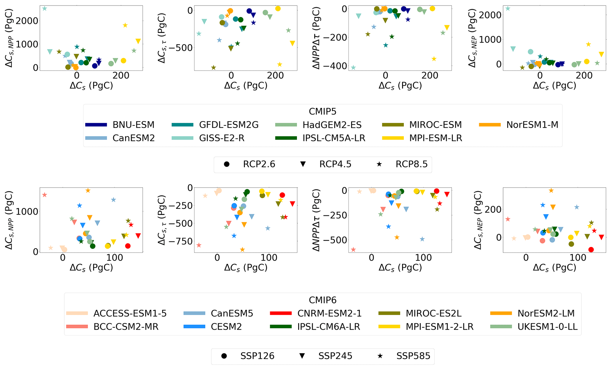
Figure A1 Scatter plot comparing the relationship between ΔC_s,NPP, ΔC_s,τ, ΔNPPΔτ_s, and $\mathrm{\Delta }{\mathrm{C}}_{\mathrm{s},{\mathit{\tau }}_{\mathrm{NEP}}}$, each against ΔC_s for CMIP5 (top row) and CMIP6 (bottom row) ESMs for future scenarios SSP126 and RCP2.6, SSP245 and RCP4.5, and SSP585 and RCP8.5.

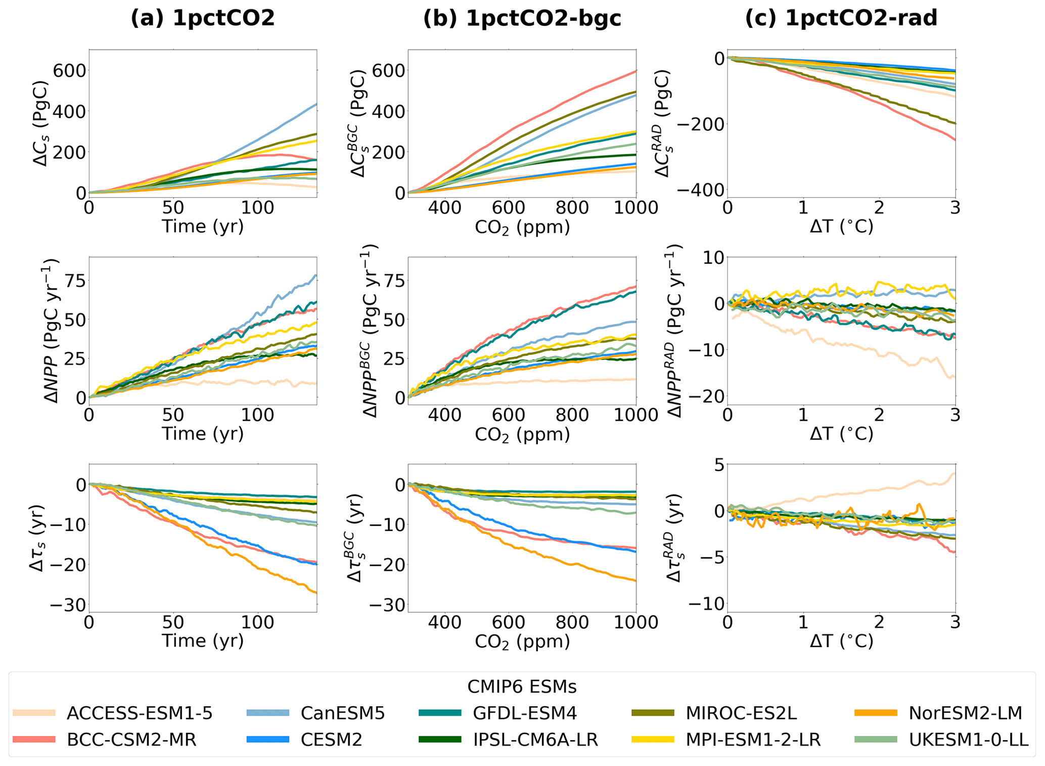
Figure A2 Time series of projected changes in soil carbon (ΔC_s, top row), net primary productivity (ΔNPP, middle row), and soil carbon turnover time (Δτ_s, bottom row) in CMIP6 ESMs for the idealised simulations 1 % CO₂ (a), biogeochemically coupled 1 % CO₂ (BGC, b), and radiatively coupled 1 % CO₂ (RAD, c).

Table A1 Table presenting the absolute (Pg C) and relative (%) changes in 21st century soil carbon for each CMIP5 model and the ensemble mean ± standard deviation, for each future RCP scenario.

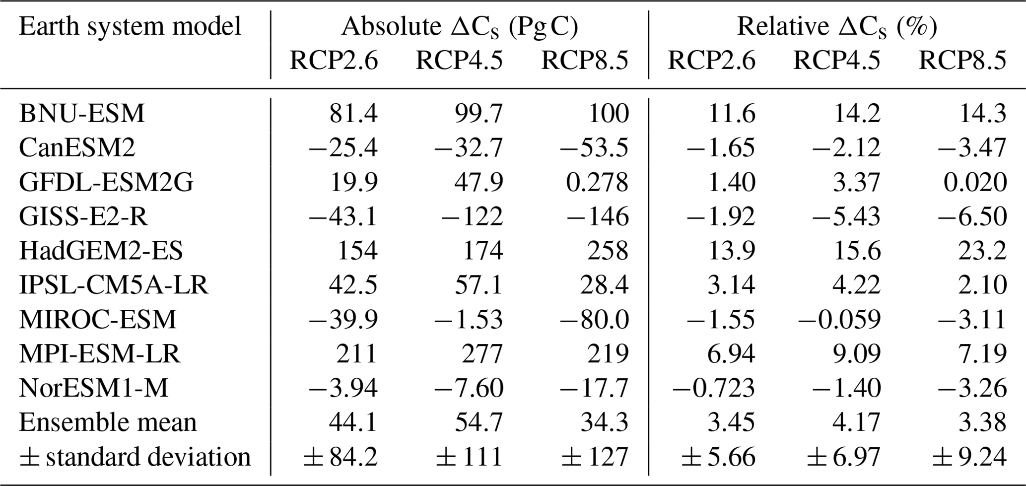
Table A2 Table presenting the changes in 21st century NPP and τ_s for each CMIP5 model and the ensemble mean ± standard deviation, for each future RCP scenario.