the Creative Commons Attribution 4.0 License.
the Creative Commons Attribution 4.0 License.
 | 28 Jun 2024
Separating above-canopy CO2 and O2 measurements into their atmospheric and biospheric signatures
Jordi Vilà-Guerau de Arellano
Raquel González-Armas
Bert G. Heusinkveld
Ivan Mammarella
Wouter Peters
Ingrid T. Luijkx
Atmospheric tracers are often used to interpret the local CO2 budget, where measurements at a single height are assumed to represent local flux signatures. Alternatively, these signatures can be derived from direct flux measurements or by using fluxes derived from measurements at multiple heights. In this study, we contrast interpretation of surface CO2 exchange from tracer measurements at a single height to measurements at multiple heights. Specifically, we analyse the ratio between atmospheric O2 and CO2 (exchange ratio, ER) above a forest. We consider the following two alternative approaches: the exchange ratio of the forest (ERforest) obtained from the ratio of the surface fluxes of O2 and CO2 derived from measurements at multiple heights, and the exchange ratio of the atmosphere (ERatmos) obtained from changes in the O2 and CO2 mole fractions over time measured at a single height. We investigate the diurnal cycle of both ER signals to better understand the biophysical meaning of the ERatmos signal. We have combined CO2 and O2 measurements from Hyytiälä, Finland, during spring and summer of 2018 and 2019 with a conceptual land–atmosphere model to investigate the behaviour of ERatmos and ERforest. We show that the CO2 and O2 signals as well as their resulting ERs are influenced by climate conditions such as variations in soil moisture and temperature, for example during the 2018 heatwave. We furthermore show that the ERatmos signal obtained from single-height measurements rarely represents the forest exchange directly, mainly because it is influenced by entrainment of air from the free troposphere into the atmospheric boundary layer. The influence of these larger-scale processes can lead to very high ERatmos values (even larger than 2), especially in the early morning. These high values do not directly represent carbon cycle processes, but are rather a mixture of different signals. We conclude that the ERatmos signal provides only a weak constraint on local-scale surface CO2 exchange, and that ERforest above the canopy should be used instead. Single-height measurements always require careful selection of the time of day and should be combined with atmospheric modelling to yield a meaningful representation of forest carbon exchange. More generally, we recommend always measuring at multiple heights when using multi-tracer measurements to study surface CO2 exchange.
- Article
(3512 KB) - Full-text XML
- BibTeX
- EndNote


Rising atmospheric CO2 levels resulting from fossil fuel combustion and land-use change emissions, which are moderated by uptake by the terrestrial biosphere and oceans, require comprehensive assessment of carbon exchange at local and global scales (Friedlingstein et al., 2022). Atmospheric O2 serves as a valuable tracer, enhancing our understanding of carbon exchange due to the close linkage between O2 and CO2 in carbon cycle processes such as fossil fuel combustion, photosynthesis, and respiration (Manning and Keeling, 2006; Worrall et al., 2013; Keeling and Manning, 2014; Bloom, 2015; Hilman et al., 2022). The exchange ratio (ER ), denoted as the number of moles of O2 exchanged per mole of CO2, represents the specific link between O2 and CO2 for different processes (Keeling et al., 1998). Long-term O2 and CO2 measurements allow us to derive the global ocean carbon sink (Stephens et al., 1998; Rödenbeck et al., 2008; Tohjima et al., 2019) and to estimate changes in fossil fuel emissions (Pickers et al., 2022; Ishidoya et al., 2020; Rödenbeck et al., 2023).
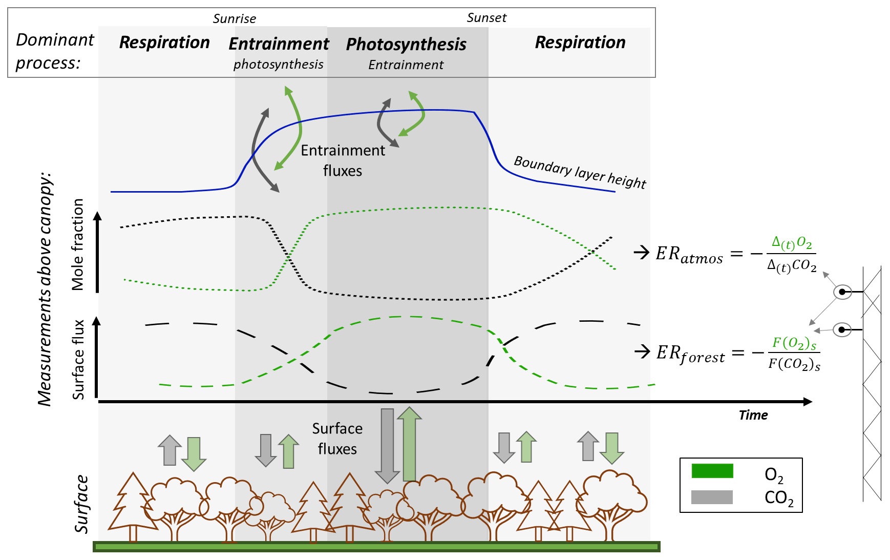
Figure 1Schematic overview of diurnal cycles of the surface fluxes and mole fractions of atmospheric O2 and CO2 above a forest canopy. The figure illustrates the dominant processes throughout the day, with forest exchange dominating the nocturnal and afternoon periods, while early morning signals are primarily influenced by entrainment of air from the residual layer or the free troposphere. The surface fluxes of O2 and CO2 result in the exchange ratio signal of the forest (ERforest), while the changes in the mole fractions of O2 and CO2 over time can lead to variations of the exchange ratio signal of the atmosphere (ERatmos). Note that the term “surface fluxes” refers to the fluxes from the surface layer, which includes the vegetation layer including the top of the canopy. The surface layer is the lowest 10 % of the boundary layer, where the surface directly influences the atmospheric boundary layer.
For global applications, a constant ER of 1.1 (mol mol−1) is assumed for the terrestrial biosphere (Severinghaus, 1995). However, the ER of terrestrial biosphere exchange is not uniform at smaller scales; it varies between ecosystems and over time (Angert et al., 2015; Bloom, 2015; Battle et al., 2019; Hilman et al., 2022). Measuring the ERs of ecosystems and the underlying gross processes facilitates the partitioning of net ecosystem exchange (NEE) into gross primary production (GPP) and total ecosystem respiration (TER) (Ishidoya et al., 2015; Faassen et al., 2023), which is still challenging (Reichstein et al., 2005). The ER for net ecosystem exchange can be determined from the ratio of the net turbulent surface fluxes of O2 and CO2 above the canopy, referred to as ERforest (see Fig. 1). The O2 surface fluxes can be inferred from the vertical gradient: the difference between O2 mole fraction measurements at multiple heights, together with a turbulent exchange coefficient. Currently, available instruments do not allow eddy covariance (EC) O2 measurements. The ERforest signal predominantly represents forest exchange occurring in and below the canopy (small-scale processes), comprising the individual ERs of TER (ERr) and GPP (ERa) (Ishidoya et al., 2013, 2015; Faassen et al., 2023). Alternatively, the net ecosystem ER has been estimated based on measurements of O2 and CO2 mole fractions in the atmosphere at a single height above the canopy. This is referred to as ERatmos (Fig. 1) and is defined as the change in O2 and CO2 mole fractions over time (Seibt et al., 2004; Battle et al., 2019; Faassen et al., 2023).
In our recent study (Faassen et al., 2023), we presented a comprehensive comparison of the diurnal behaviour of ERforest and ERatmos using measurements collected above a boreal forest in Hyytiälä, Finland. Our analysis revealed that during the afternoon (the photosynthesis-dominant period in Fig. 1), the ERatmos signal approaches the ERforest value, although they did not converge completely. Furthermore, we showed that during the entrainment-dominant period (see Fig. 1), the ERatmos signal strongly exceeded the expected ER value for biosphere exchange, which is typically around 1.1 (Severinghaus, 1995), and even surpassed 2.0. Such high ER values (>2.0) cannot be attributed to a single process such as photosynthesis, respiration, or fossil fuel combustion, as their ER values are below 2.0. We proposed that the high ERatmos signal was likely influenced by large-scale processes, specifically the entrainment of air from the free troposphere into the boundary layer (Faassen et al., 2023). Seibt et al. (2004) and Yan et al. (2023) also argue that ERatmos cannot capture the ER signal of a forest. In contrast, in the studies by Ishidoya et al. (2013, 2015), ERforest and ERatmos do result in similar values when small-scale processes dominate over large-scale processes. In Faassen et al. (2023), we concluded that an atmospheric model was needed to interpret the observed diurnal signals of ERatmos and ERforest. The current study delivers this model-based analysis.
Until now, atmospheric O2 above forest canopies has primarily been modelled with relatively simple one-box models that use only the surface components, lacking implementation of boundary layer dynamics such as entrainment and boundary layer growth (Seibt et al., 2004; Ishidoya et al., 2013). Understanding how mole fractions and, consequently, how ERatmos evolves throughout the day requires accounting for these critical processes. Yan et al. (2023) recently modelled O2 and CO2 within and below a canopy using a multi-layer model and showed that ERatmos and ERforest have diurnal and annual patterns. However, ERatmos was treated as a constant value above the canopy and boundary layer dynamics were not accounted for. To expand on the work by Yan et al. (2023) and gain further insight into the diurnal ERatmos behaviour above a canopy, in this study, we use the mixed-layer Chemistry Land-surface Atmosphere Soil Slab (CLASS) model (Vilà-Guerau de Arellano et al., 2015). In short, the model is able to represent the thermodynamics and biophysical processes associated with the diurnal variation in the boundary layer and can provide insights into the processes contributing to ERatmos formation. Additionally, the model facilitates the analysis of ERatmos behaviour under more extreme conditions such as droughts or heatwaves.
In this study, we aim to enhance our understanding of single-height O2 and CO2 measurements and the resulting ERatmos signal, as observed above the canopy, and we propose a new relationship between the ERatmos and ERforest signal. We seek to determine whether single-height O2 and CO2 measurements can be employed to estimate the ecosystem's ER despite the aforementioned limitations. Additionally, we explore whether the ERatmos signal constrains boundary layer dynamics, and we identify cases where large-scale processes (e.g. entrainment of background air) influence the signal of small-scale processes (e.g. NEE) by analysing different diurnal regimes of ERforest and ERatmos. We combine measurements from campaigns in Hyytiälä, Finland, during spring and summer of 2018 and 2019 with an analysis of the mixed-layer CLASS model. This combined approach allows us to address the following research questions: (1) when does ERatmos represent local forest exchange processes and become equal to ERforest and (2) what is the underlying physical explanation for the high ERatmos values observed in the recent study by Faassen et al. (2023)?
In this paper we first derive a theoretical relationship between ERatmos and ERforest that can help us to understand which components influence the diurnal cycle of ERatmos and when ERatmos should indicate the same processes as ERforest (Sect. 2). To evaluate the diurnal cycle of ERatmos we combine observational data with the CLASS model (Sect. 3). We then show the model evaluation and the ERatmos and ERforest model results in Sect. 4.2, and we analyse different cases to explain the diurnal behaviour of ERatmos during distinct periods of the day and investigate when ERatmos represents forest exchange (Sect. 4.3). Next, we place our results in perspective and show how ERatmos should (not) be used (Sect. 5). Finally, we present our conclusions on the physical explanations for the differences between the diurnal behaviour of both ERatmos and ERforest.
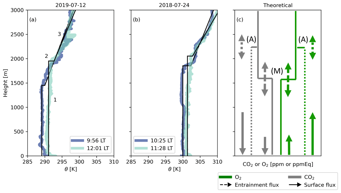
Figure 2Vertical profiles of potential temperature (θ) measured by radiosondes at Hyytiälä on 12 July 2019 (a) and 24 July 2018 (b). The observations are conceptualized (black lines) to show (1) the well-mixed profiles at different time steps, (2) the jumps between the boundary layer and the free troposphere, and (3) the lapse rate in the free troposphere; 1, 2, and 3 are used to initialize the CLASS model. Panel (c) gives the theoretical vertical profiles of O2 and CO2 for the early morning (M) and late afternoon (A). The sizes of the arrows indicate the effects of entrainment (dashed lines) and the surface fluxes (solid lines) on the vertical profiles.
2.1 The mixed-layer theory
The CLASS land–atmosphere model (Vilà-Guerau de Arellano et al., 2015) is based on the mixed-layer theory which assumes that scalars (such as O2, CO2, θ) are constant with height in the atmospheric boundary layer (Lilly, 1968; Tennekes, 1973). Figure 2 illustrates these assumptions for potential temperature (θ), O2, and CO2. Within the mixed-layer theory, no distinct surface layer exists, and a capping inversion links the mixed-layer value (the bulk constant value) with the lapse rate of the free troposphere. This inversion, termed the “jump” (Δ(ft-bl)), represents the difference of a scalar (e.g. the CO2 mole fraction) between the atmospheric boundary layer and the free troposphere. The free troposphere is represented by a linear change of the scalar with height (the lapse rate).
CLASS describes the well-mixed layer with a scalar constant in height (Fig. 2). This scalar (ϕ) can then be solved in the mixed layer with the following equation (Vilà-Guerau de Arellano et al., 2015):
where ∂ϕ/∂t is the tendency (i.e. change over time) of a generic well-mixed scalar, w′ are the deviations of the mean for w which is the vertical wind speed, and ϕ′ are the deviations from the mean for a scalar ϕ. The term is the surface flux of ϕ and represents the small-scale processes, is the entrainment flux, h is the boundary layer height, and adv(ϕ) is the horizontal advection of scalar ϕ into the well-mixed layer. In contrast to the local surface exchange, and adv(ϕ) represent large-scale processes.
The entrainment flux is dependent on the entrainment velocity and the jump:
where we is the entrainment velocity, Δ(ft-bl)ϕ is the jump between the free troposphere and the atmospheric boundary layer, and wsub is the mean vertical subsidence velocity normally associated with high-pressure systems. We assume wsub to be negligible, because our focus does not lie on the influence of synoptic scale processes.
Δ(ft-bl)ϕ changes over time (see Fig. 2) and depends on the surface fluxes and the air that is entrained from the free troposphere (see Eq. 1):
where γϕ is the lapse rate of ϕ in the free troposphere and is the change over time of the well-mixed scalar ϕ (i.e. in the boundary layer).
Lastly, the growth of the boundary layer height effectively determines the entrainment velocity and therefore the entrainment flux of a certain scalar. The growth of the boundary layer is caused by the virtual potential temperature (θv), also called buoyancy:
where θv is the virtual potential temperature (i.e. potential temperature of dry air) and wsub is the subsidence velocity. For more details on these equations, see Vilà-Guerau de Arellano et al. (2015) and Sect. 3.2.2 and Appendix A2 for the application of O2.
2.2 Theoretical relationship between ERatmos and ERforest
The ER signal of the forest (ERforest) is defined as (Faassen et al., 2023)
where and are the mean net turbulent surface fluxes of O2 and CO2, respectively, over a certain time period above the canopy and can be derived from the vertical gradient of O2 (Δ(z)O2) and CO2 (Δ(z)CO2) measurements at two heights together with an exchange coefficient following the K-theory (Kϕ) (Faassen et al., 2023). Note that the K-theory does not apply when one of the measurement levels is inside the canopy. For readability, we write the surface fluxes for both O2 and CO2 as Fϕ, instead of that was used above for the general theory.
The ER signal of the atmosphere (ERatmos) is defined as (Faassen et al., 2023)
where Δ(t)O2 and Δ(t)CO2 are the changes in the O2 and CO2 mole fractions over time (tendencies) at a single height. Linear regression between O2 and CO2 can be applied, and the slope gives the ERatmos value for a certain event or time period. For this study, linear regression was applied for the three periods described in Sect. 4.2.1 for the observations (1 value per 30 min) and the CLASS model output (1 value per 10 s).
According to the mixed-layer theory described above, the tendencies in Eq. (6) depend on the surface and entrainment fluxes, together with the boundary layer height (h) (see Eq. 1). Equation (6) can be rewritten by implementing Eq. (1):
where and are the net surface fluxes of O2 and CO2, and and are the entrainment fluxes of O2 and CO2, respectively. For simplicity, we ignored the advection term in Eq. (1) here, but we will add it later (Eq. 9). As shown in Eq. (2), the entrainment flux depends on the entrainment velocity (we) and the jump between the free troposphere and the boundary layer (Δ(ft-bl)ϕ). Combining the definition of ERforest (Eq. 5) with Eq. (2) allows us to rewrite Eq. (7) as
where Δ(ft-bl)O2 and Δ(ft-bl)CO2 are the jumps of O2 and CO2 between the free troposphere and the boundary layer, and βϕ is the ratio between the entrainment flux and the surface flux (Vilà-Guerau de Arellano et al., 2004). Equation (8) shows a clear relationship between ERatmos and ERforest following the mixed-layer theory.
Using the definition of Eq. (1), we can extend Eq. (8) to include the effect of advection of O2 (adv) and CO2 (adv), which is, next to entrainment, the second important large-scale process influencing the O2 and CO2 values:
Note that in this paper, we mostly focus on cases without advection. We include it here for completeness and discuss the influence of advection in Sect. 5.2.
In Appendix A1 we analyse Eq. (8) by determining when ERatmos would theoretically be close to ERforest during the day. We show that the β values are of particular importance here: when the β's of O2 and CO2 are equal or very small, ERatmos gives the same signal as ERforest. To fully unravel the diurnal variations of ERatmos under realistic conditions and identify influencing factors, we need to analyse a real case. Therefore, we study two observed situations by means of the CLASS coupled land–atmosphere model, which we will describe in Sect. 3.2.
In this section we describe the measurements that were used in this study, together with the mixed-layer model used to evaluate the ERatmos and ERforest signals.
3.1 Hyytiälä 2018 and 2019 measurement campaigns
The observational data were obtained from the SMEAR II Forestry Station of the University of Helsinki in Finland, located in Hyytiälä, Finland (61°51′ N, 24°17′ E, +181 MSL) (Hari et al., 2013). The SMEAR II station serves as a measurement site within a boreal forest equipped with a 128 m tower for continuous measurements of atmospheric variables, fluxes, and greenhouse gas mole fractions. These data are accessible at https://smear.avaa.csc.fi/ (last access: 24 June 2024). The tower is situated in a homogeneous Scots pine forest, with an average canopy height of 18 m and podzolic soil. The measurement site is predominantly influenced by the surrounding forest and is minimally impacted by signals of fossil fuel combustion (Faassen et al., 2023). For a comprehensive description, see Hari et al. (2013).
During the spring and summer of 2018 (3 June until 2 August) and 2019 (10 June until 17 July), two measurement campaigns, referred to as OXHYYGEN (Oxygen in Hyytiälä), were conducted at Hyytiälä. Continuous measurements of both O2 and CO2 mole fractions were taken at two heights (125 and 23 m). O2 was measured using an Oxzilla II fuel cell analyser, and CO2 was measured with a non-dispersive infrared (NDIR) photometer (URAS26). Further details on these measurements and the measurement systems are given in Faassen et al. (2023). The measurement precision for O2 was 19 per meg, and for CO2 it was 0.07 ppm. Although the precision for O2 is relatively poor compared to previous studies, it is still adequate for studying the diurnal timescale, as shown in Faassen et al. (2023).
O2 measurements are typically expressed as δO2 / N2 ratios in per meg units due to the high abundance of O2 in the atmosphere (20.946 %) classifying it as a non-trace gas. For direct comparison with CO2 and implementation into our model, we convert per meg to ppm equivalents (ppmEq) by multiplying with the standard mole fraction of O2 in air of 0.20946 (Keeling et al., 1998).
During the OXHYYGEN campaigns, radiosondes were launched on multiple days several times per day to quantify the impact of boundary layer dynamics on the O2 and CO2 diurnal cycles. The radiosondes (Windsond, model S1H3-R, Sweden) measured vertical profiles of air pressure, wind speed, wind direction, relative humidity, and temperature, with flight heights reaching a maximum of 4500 m and rising rate of about 1.7 m s−1. The measurements have an accuracy of 1.0 hPa for air pressure, 5 % for wind speed, 0.2 °C for temperature, and 1.8 % for relative humidity. The temperature and humidity probe has a response time of 6 s, effectively averaging over about 10 m of altitude. For our analysis, we computed vertical profiles of potential temperature (θ) and specific humidity (q) based on pressure, temperature, and relative humidity measurements. Based on the vertical profile of vertical temperature, we also determine the boundary layer height with the parcel method (Kaimal and Finnigan, 1994). Figure 2 shows examples of vertical profile measurements of θ for 12 July 2019 and 24 July 2018.
3.2 Modelling setup in CLASS
3.2.1 Implementation of CO2 in CLASS
CLASS serves as a fundamental tool that enables further understanding of specific processes within the atmospheric boundary layer. Several studies have shown that CLASS is successful in reproducing observational data (Vilà-Guerau de Arellano et al., 2012, 2019; Schulte et al., 2021). The study of Ouwersloot et al. (2012) specifically showed that CLASS is able to reproduce the boundary dynamics at the Hyytiälä measurement site. Within CLASS, the vegetation is described using a big-leaf model. The surface stomatal conductance that is representative for the canopy is up-scaled from leaf stomatal conductance by integrating over the leaf area index and incorporating soil moisture. The leaf stomatal conductance is calculated with the A-gs model. The A-gs model relates leaf stomatal conductance (gs) to the net leaf CO2 assimilation (A) (Jacobs et al., 1996; Ronda et al., 2001). The model computes the dependence of gs and A on the internal CO2 mole fraction, the amount of light, the atmospheric temperature, the vapour pressure deficit, and the soil water content at the root zone. Finally, the canopy net CO2 assimilation is obtained with a function that is inspired by Fick's law of diffusion, based on the difference in the atmospheric CO2 and internal CO2 mole fractions, the aerodynamic resistance, and the surface stomatal conductance. The soil respiration is implemented as a function of soil temperature and soil moisture (Vilà-Guerau de Arellano et al., 2012). Combining the net assimilation (An) of the plants at canopy level and the soil respiration flux results in the net ecosystem exchange (NEE). This means that the model does not produce exactly the GPP and TER fluxes. The differences between An and GPP, and soil respiration and TER, are not directly relevant for our study and we therefore refer to GPP and TER in the following sections, as these terms are more commonly used in the atmospheric CO2 community. The water cycle is connected to the CO2 cycle through the surface stomata and the soil moisture inhibition functions for assimilation and respiration.
3.2.2 Implementation of O2 in CLASS
To model both ERforest and ERatmos, we incorporated the surface flux and the atmospheric mole fraction of O2 into the CLASS model. We represent the surface flux of O2 by multiplying the ER of assimilation (ERa) and the ER of respiration (ERr) with the CLASS-calculated CO2 fluxes at the canopy scale. We used the observationally derived ERa and ERr values as previously determined in Faassen et al. (2023) for the same site, which were 0.96 and 1.03, respectively. The net surface flux of O2 was then resolved with the following equation:
where F(O2)s is the net O2 surface flux above the canopy, is the net assimilation flux, and is the soil respiration flux. The change of atmospheric O2 over time was resolved with Eq. (A1) (similar to Eq. 1) and the entrainment flux is based on Eq. (A2) (see also Eq. 2). Note that the ERa from Faassen et al. (2023) was based on GPP fluxes, and this ERa is now linked to the net assimilation flux (GPP minus the photo- and dark respiration) of the model (Jacobs et al., 1996; Ronda et al., 2001). Seibt et al. (2004) and Ishidoya et al. (2013) showed that ERa values based on net assimilation have similar values compared to the 0.96 based on GPP. We therefore do not expect this discrepancy to influence our results.
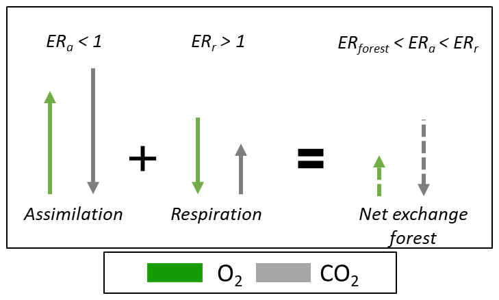
Figure 3Schematic overview of how two processes with different ER signals produce a combined ER signal that is not necessarily the average of the two processes nor necessarily falls within the range of the two combined ER signals. This is due to the different signs of the O2 and CO2 fluxes. The example is given for combining the ER signal of assimilation (ERa) and respiration (ERr) into ERforest and uses values from our study that are by coincidence larger and smaller than 1.
It is important to note that the resulting ERforest signal is not the (weighted) average between ERa and ERr, as was also shown by Faassen et al. (2023). The ERforest signal results from the TER and GPP fluxes with different sizes and signs, each with their own ER signals (ERr and ERa, respectively). Figure 3 shows that the resulting ERforest signal does not necessarily fall within the range of the ERa and ERr signals, because the TER and GPP have opposite signs of the O2 and CO2 fluxes. This counter-intuitive situation can also occur for combining signals with different isotopic signatures (Miller and Tans, 2003).
3.2.3 Initial conditions
We determined initial and boundary conditions for two cases to constrain the model to the observations. One case was based on the year 2019 (base case) and the other case was based on the year 2018 (characterized by a warm summer in Finland; Peters et al., 2020; Lindroth et al., 2020). Using the two years to initialize CLASS, we were able to better constrain the vegetation's response in the CLASS model under extreme conditions. For each year, we selected one representative day for initialization and validation of the CLASS model. We used 10 July 2019 for the base case and an aggregate between 28 and 29 August 2018 for the warm case. The initial and boundary conditions for initialization of the CLASS runs can be found in Tables C2 and C3 in the Appendix. Note that the initial jumps (Δ(ft-bl)) of O2 and CO2 are based on the best fit between the model and the observations during the day, as direct observations of the jumps were not available. A detailed discussion can be found in Sect. 5.3.
We deliberately made only minimal adjustments for the initialization of the 2018 case compared to the 2019 base case to ensure consistency. We assumed that the initial relative humidity remained constant at 80 % regardless of temperature variations, similar to the studies of Vilà-Guerau de Arellano et al. (2012) and van Heerwaarden and Teuling (2014).
We adjusted several parameters of the A-gs land–surface scheme and the soil respiration to improve the agreement between the surface fluxes of the model and the observations in Hyytiälä for both the base case (2019) and the warmer case (2018) (Table C2). We decreased the mesophyll conductance (gm: 2 mm s−1) to better match pine forest conditions (Gibelin et al., 2008; ECMWF IV, 2014; Visser et al., 2021). Furthermore, the reference temperature of gm (: 305 K) was increased to reduce afternoon plant stress and to make the CLASS run more comparable with the observations. Lastly, we adjusted the curvature of the drought-response curve (cβ) from zero to 15 % (Combe et al., 2015), given that several studies have demonstrated the pine forest in Hyytiälä to be relatively resilient to lower soil moisture values, thus necessitating a higher (cβ) value (Gao et al., 2017; Lindroth et al., 2020).
3.2.4 Sensitivity analyses
We conducted two sensitivity analyses to gain a deeper understanding of the ERatmos behaviour under varying conditions and to identify factors that lead to a smaller difference between ERatmos and ERforest. Specifically, we looked at changes in ERatmos resulting from changing the different components of Eq. (8). The first sensitivity analysis uses the 2019 base case and investigates the effect of background air with a different composition by altering the initial jumps of O2 and CO2. By changing only the initial jump and keeping the rest of the 2019 case the same, we simulate situations in which the free troposphere mole fractions of O2 and CO2 have changed. In the second sensitivity analysis we examined the impact of climate conditions by modifying the soil moisture and air temperature, mimicking the conditions observed during the 2018 heatwave. Table C1 presents the variables used for initializing four cases for these two sensitivity studies.
In this section, we first show our results for the validation of the CLASS model using observations (Sect. 4.1). Subsequently, we discuss the diurnal variability of both the ERforest and ERatmos signals (Sect. 4.2). We identify three distinct periods throughout the day in which ERatmos shows large variability (Sect. 4.2.1). We address the large ERatmos that we find in both the observations and the model results (Sect. 4.2.2). Finally, we perform sensitivity analyses to study the effects of changing large-scale conditions, in order to show that our findings are not only valid for a single day (Sect. 4.3).
4.1 Validation of the O2 and CO2 model results
Overall, the modelled O2 and CO2 diurnal cycles match well with the observational data. Figures A3 and A2 in Appendix A3 show that CLASS accurately reproduces the diurnal cycles and captures the O2 mole fraction changes on a daily timescale for both 2018 and 2019 (Fig. A3b and c). The figure shows that the differences between the two years are relatively small and indicate that the boundary layer dynamics and the surface fluxes are well represented in CLASS. To accurately replicate the rapid decrease of CO2 and the sharp increase of O2 during the rapid growth of the atmospheric boundary layer (between 06:30 and 11:30), we adjusted the jump between the boundary layer and the free troposphere (Δ(ft-bl)) for both O2 (30 ppmEq) and CO2 (8 ppm), ensuring that the model aligned with the measurements. Based on values from previous studies, it is realistic for the CO2 jump to range between 8 and 40 ppm (Vilà-Guerau de Arellano et al., 2004; Casso-Torralba et al., 2008). While there are limited data available to validate the jump of O2, based on preliminary results of a campaign in Loobos, the Netherlands, a jump of 30 ppmEq for O2 seems reasonable. Our chosen combination of O2 and CO2 jumps remains an uncertain component in our analysis and will be further discussed in Sect. 5.3.
4.2 Diurnal variability of ERatmos and ERforest in 2018 and 2019
In this section we discuss the diurnal variability of the ERatmos signal for the 2018 and 2019 cases. First we focus on the budget components (GPP, TER, and entrainment) that influence the O2 and CO2 signals (Sect. 4.2.1). To complete the analysis, we support the numerical analysis with Eq. (8) to gain a more comprehensive understanding of the underlying processes driving the ERatmos signal for the 2019 case (Sect. 4.2.2).
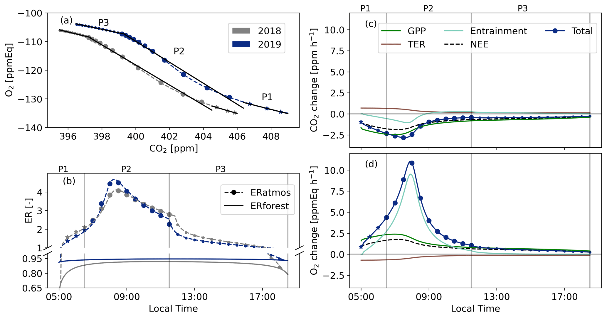
Figure 4Diurnal cycles of O2 and CO2 mole fractions (a) and ERatmos and ERforest (b) as modelled with CLASS for the selected days in 2018 and 2019. We identify three distinct periods based on panels (c) and (d), which show the tendencies for the 2019 case (change over time) for CO2 and O2 for each process that influences their mole fractions (Eq. 1): P1 05:00–06:30, P2 06:30–11:30, and P3 11:30–18:30 LT. The symbols represent half-hourly averaged values of the CLASS model output.
4.2.1 The three distinct periods of the ERatmos signal during daytime
The ERatmos signals obtained for the 2018 and 2019 experiments display large variability throughout the daytime (panels a and b in Fig. 4). We identify three distinct periods during the day based on the processes shown in Fig. 4c and d: (1) the early morning regime (P1, 05:00–06:30 LT) characterized by an increasing net CO2 flux into the forest but a non-growing boundary layer (Fig. A3a), during which the ERatmos signal during P1 is still relatively close to ERforest; (2) the entrainment-dominant period (P2, 06:30–11:30 LT), where air from a residual layer or air masses from the free troposphere are entrained into the boundary layer and significantly influence the signals, leading to large ERatmos values with an average greater than 3 and extreme values reaching close to 5; (3) the afternoon period (P3, 11:30–18:30 LT), where surface processes dominate the observed signals and ERatmos moves slowly back towards ERforest and becomes more consistent with values expected for surface processes. The ERatmos values during the three identified periods show good agreement between the observations and the model results (Table 1). This analysis confirms from a model perspective that values above 2 for ERatmos, as we reported in Faassen et al. (2023), are indeed possible. Figure 4c and d give first indications of what could cause these high values for ERatmos: high influence of entrainment and a different behaviour of the tendencies that influence O2 compared to CO2. In the next section we discuss the diurnal behaviour of ERatmos in more detail by using Eq. (8).
We find that ERforest is much less variable throughout the day than ERatmos (Fig. 4b). In the early morning and later afternoon, the ERforest value is lower than during the midday period. This is caused by a TER flux (with a higher ER signal) almost equal to the GPP flux (with a lower ER signal) caused by low sunlight (Fig. 3). At midday, the assimilation of CO2 by the canopy, with a lower ER signal, becomes increasingly dominant, causing the ERforest signal to move closer to the ERa value.
Table 1ERatmos (calculated as the slope of the O2 and CO2 mole fractions) and ERforest values for the selected days in 2018 and 2019 for both observations (Obs) and the CLASS model for the three selected periods (P1: 05:00–06:30, P2: 06:30–11:30, and P3: 11:30–19:30 LT). The uncertainties in the observed ERatmos and ERforest signals are determined following Faassen et al. (2023). Note that due to limited observational data, we were unable to derive ERatmos values for P1 and P2 in 2018 and for P1 in 2019. NA signifies not available.
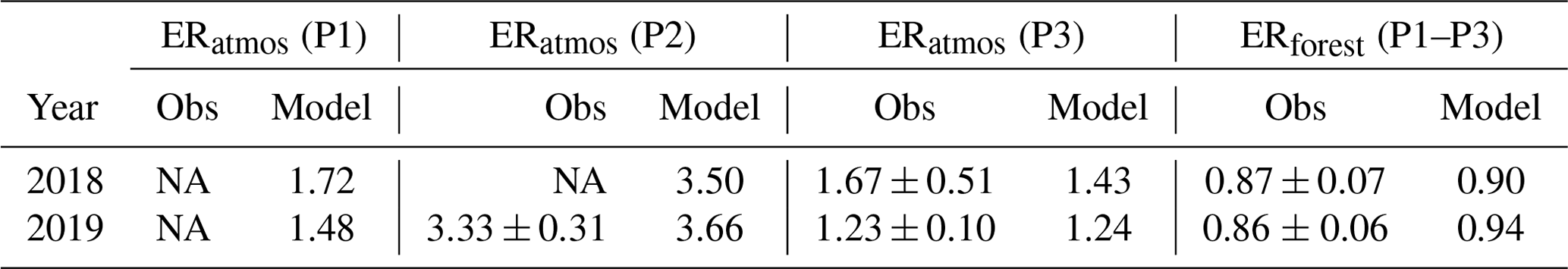
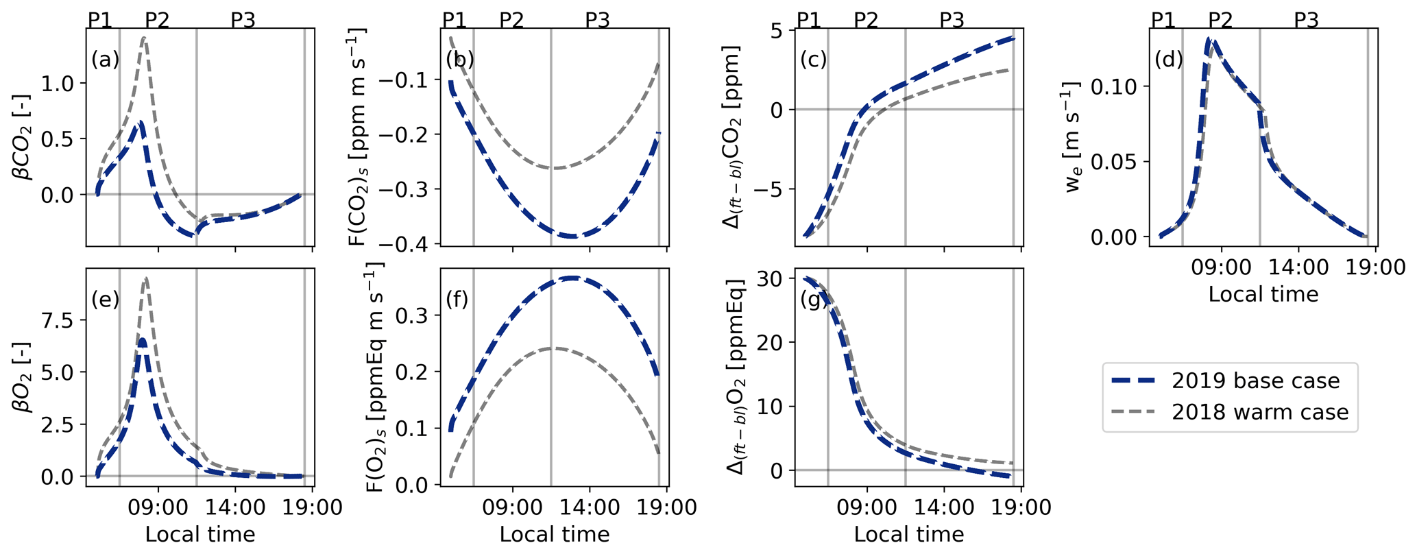
Figure 5Diurnal variability of the different components of Eq. (8) for the base case (2019) and the warm case (2018) derived using the CLASS model. Panels (a) and (e) show the β values for CO2 and O2, where β is the entrainment flux divided by the surface flux (Eq. 8); panels (b) and (f) show the net surface flux; panels (c) and (g) show the jumps between the free troposphere and the boundary layer (Δ(ft-bl)); and panel (d) shows the entrainment velocity (we). The vertical lines represent three distinct periods: 05:00–06:30 (P1), 06:30–11:30 (P2), and 11:30–18:30 LT (P3).
4.2.2 Explanation of the large ERatmos values
Analysing the diurnal cycle of the different components of Eq. (8) for the 2019 case reveals that the peak value of ERatmos during P2 is caused by the higher β values (the entrainment flux divided by the surface flux) for O2 compared to CO2 (Fig. 5). The difference between and is a result of the high Δ(ft-bl)O2 Δ(ft-bl)CO2 ratio (higher than 3). The terms Δ(ft-bl)O2 and Δ(ft-bl)CO2 represent the jump across the boundary layer top, and each has a different diurnal cycle caused by a different surface flux (Fig. 5c and g). The different diurnal cycles for the jumps lead to an increase in the Δ(ft-bl)O2 Δ(ft-bl)CO2 ratio, consequently raising the ratio between the β values. This effect is further amplified by a higher surface flux of CO2 compared to O2, caused by an ERforest value that is slightly lower than 1. The peak value of ERatmos during P2 occurs when both we and the Δ(ft-bl)O2 Δ(ft-bl)CO2 ratio are high and the surface fluxes are still relatively low. This combination contributes to the distinctive peak in ERatmos observed during P2.
Later in the afternoon (P3), both β values gradually decrease and become similar, resulting in an ERatmos signal that becomes closer to ERforest. This indicates that ERatmos becomes more representative for surface processes (see also Appendix Sect. A1). This decrease in P3 is primarily caused by a reduction in the entrainment velocity (we) (Fig. 5d), indicating slow growth of the atmospheric boundary layer at end of the day (Fig. A3). Additionally, the β values become more similar because Δ(ft-bl)O2 moves closer to Δ(ft-bl)CO2 during this period (Fig. 5c and g), as caused by the mixing of air with the surface.
The ERatmos signals exhibit higher values than the theoretical analysis in Appendix Sect. A1, because the diurnal cycles of the components of Eq. 8 are taken into account (Fig. A1 vs. Fig. 5). Each component of Eq. (8) follows its individual diurnal cycle, leading to higher ERatmos values. Consequently, ERatmos integrates individual contributions of several processes, particularly during P2, since it is dominated by the influence of mixing with large-scale processes. Careful consideration is needed when interpreting the ERatmos signal during this period. During P3 the ERatmos signal appears to align with ERforest at the end of the day. However, in the 2019 case, this alignment was only observed for a very short period.
We find only small differences in the diurnal behaviour of the ERforest and ERatmos signals between the 2018 and 2019 cases (Figs. 4 and 5). The ERforest value is lower in 2018 compared to 2019, specifically in the early morning and at the end of the day. This can be attributed to a higher respiration flux caused by the elevated air and soil temperatures during that day in 2018 (Fig. A3e). A higher TER flux compared to the GPP flux will decrease the ERforest value (Fig. 3). While we do not have direct measurements of ERr and ERa for 2018 and 2019, it is likely that the overall diurnal cycle pattern of ERforest in Fig. 4b (low ERforest values in the morning and afternoon, higher ERforest values during midday) for both years would have remained consistent. Previous studies suggest that ERr is generally higher than ERa, even under different atmospheric conditions (Angert et al., 2015; Fischer et al., 2015; Hilman et al., 2022). The effect of a warmer and dryer environment on the ERatmos signal will be further quantified in Sect. 4.3.2 with a more extreme case.
4.3 Sensitivity analyses: effects of changing large-scale conditions
With the next two sensitivity analyses, we evaluate whether our findings for the 2019 case are exceptional or whether they can also occur under different (large-scale) conditions. We therefore analyse days with different initial conditions compared to our 2019 and 2018 cases. We focus on the effect of changes in background air (Sect. 4.3.1) and the effect of changes in climate conditions (soil moisture and air temperature, Sect. 4.3.2). With these sensitivity analyses, we show the complexity of the ERatmos signal and all the processes by which it can be influenced. Fig. 6 is used to illustrate how ERatmos is formed by the different components of Eq. (8).
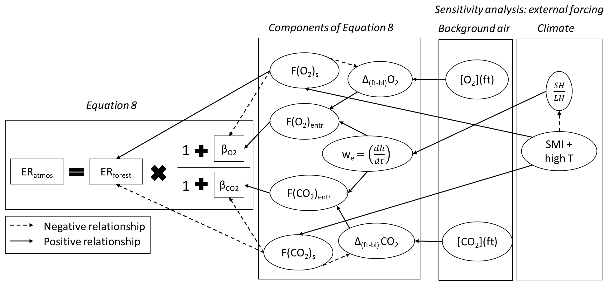
Figure 6Components of Eq. (8) and how these influence the ERatmos signal, including the exchange ratio of the forest (ERforest), the ratio between the net surface flux (Fs) and the entrainment flux (Fentr) which result in β, the jump between the free troposphere and the boundary layer (Δ(ft-bl)), and the entrainment velocity (we). The right part of the figure shows the variables that are changed in the two sensitivity analyses: the background air in the free troposphere ([O2](ft) and [CO2](ft)) and the initial soil moisture index (SMI) in combination with a high initial potential temperature (θ0), which will influence the ratio between the sensible heat flux (SH) and the latent heat flux (LH) at the surface. The dotted arrows indicate a negative influence and the solid arrows indicate a positive influence.
4.3.1 Effects of changing background air on ERatmos
Changing the background air in the free troposphere by decreasing the initial jump ratio or the jump sizes of O2 and CO2 compared to the 2019 case moves the ERatmos signal closer to ERforest during P2 and P3 (Fig. B1). A lower jump ratio than in the 2019 case but still relatively high jump values (Δ(ft-bl)O2=30 ppmEq and Δ(ft-bl)CO ppm) lead to a decrease in the peak of ERatmos during P2 and bring ERatmos closer to ERforest during P3 (yellow line in Fig. B1). As the jump ratio decreases, becomes less dominant and closer to . When the O2 and CO2 β values become closer, the ERatmos value also moves closer to ERforest (Fig. 6). However, this does not necessarily mean that the surface has become more dominant, since the Δ(ft-bl) values are still relatively high.
Reducing the jump sizes of both O2 and CO2 (Δ(ft-bl)O2=10 and Δ(ft-bl)CO) still results in a relatively high peak for ERatmos during P2 and brings ERatmos closer to ERforest during P3 (purple line in Fig. B1). Including the diurnal cycle of the jumps accounts for the effect that the CO2 jump changes from a negative to a positive value during the day. When the initial CO2 jump is lower, the sign change occurs earlier in the day and leads to a more negative value. This leads to higher ERatmos values during P2 (Fig. 6). In contrast, a lower jump size would cause the ERatmos signal to move more quickly towards ERforest during P3, because the surface fluxes dominate over the lowered entrainment flux.
Guided by our theoretical and numerical results and constrained by observations, a high ERatmos signal during the entrainment-dominant period (P2) can therefore be a result of two cases:
-
The Δ(ft-bl)O2 is substantially larger compared to Δ(ft-bl)CO2 and, therefore, dominates over .
-
Δ(ft-bl)CO2 changes sign from negative to positive and, as a result, becomes negative, resulting in a denominator closer to zero.
Changes in the background air result in a distinct change in the diurnal pattern of ERatmos. The difference between the ERatmos and ERforest signals could therefore provide extra information on the changes of large-scale processes. This is further discussed in Sect. 5.2.
4.3.2 Effect of climate conditions on ERatmos and ERforest
By studying the influence of changes in air temperature and soil moisture index (SMI: [soil moisture – wwilt]/[wfc−wwilt]) on the ERatmos signal (see Fig. 7), we gain insights into how climate conditions can effect ERatmos compared to ERforest. This allows us to study the effects of seasonality or future climate with dryer and warmer conditions. The 2018 case already showed how the ERatmos signal could change with decreasing SMI and increasing temperature compared to a more normal year in 2019 (Figs. 4 and 5). As a next step, we evaluate the full range of how ERatmos could change and how ERatmos compares to ERforest. Given the same net radiation, a higher SMI enhances soil respiration, photosynthesis, and latent heat fluxes, and thus decreases the sensible heat flux because of the energy balance closure. This therefore leads to smaller boundary layer growth and, as a result, decreases the entrainment velocity (see Fig. 6). In addition, higher air temperatures accelerate both photosynthesis and respiration up to a threshold (Jacobs et al., 1996), resulting in increased GPP and TER fluxes. A lower SMI in combination with higher temperatures can stress plants, leading to decreased O2 and CO2 surface fluxes and an enhanced sensible heat flux. This will increase boundary layer growth and the entrainment velocity (Eqs. 2 and 4). Note that there are also minor changes in ERforest when the SMI and air temperature change as a result of GPP and TER changes.
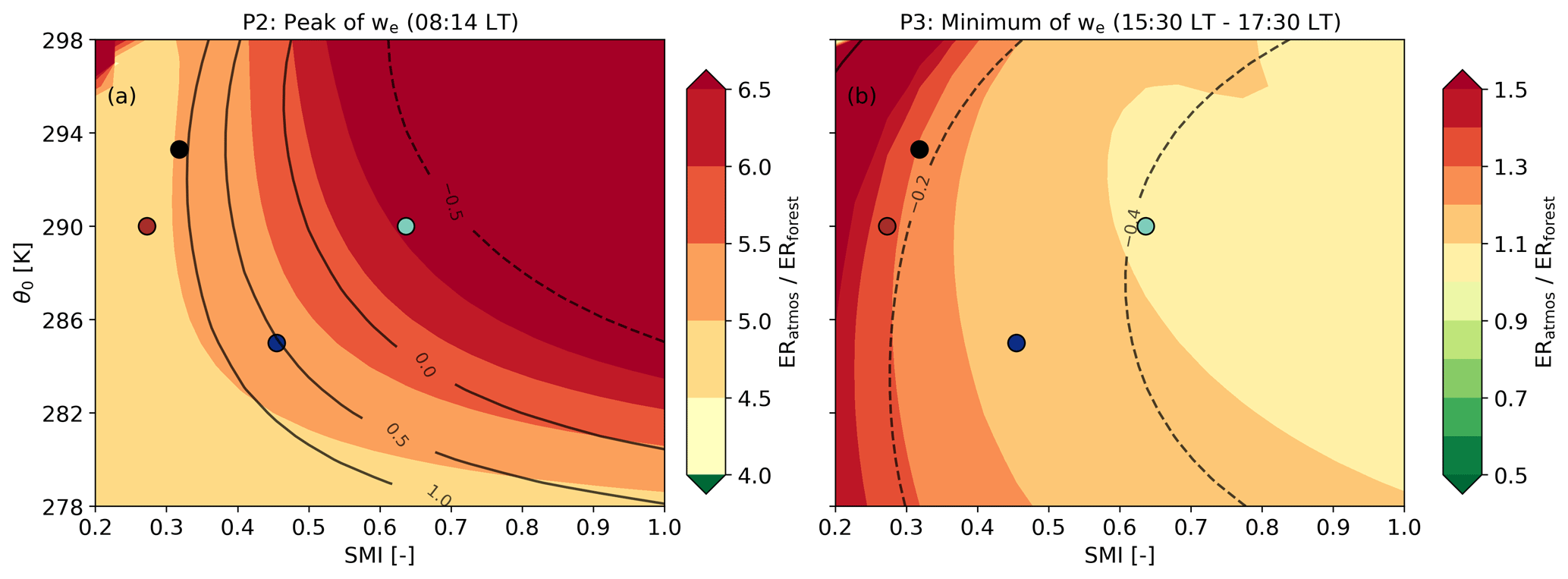
Figure 7Evaluation of the ratio between ERatmos and ERforest as a function of two key variables that show the effect of a drier and warmer climate: the soil moisture index (SMI) and the initial potential temperature (θ0). Two periods in the day are analysed: (a) during the maximum value of we at 08:14 LT (P2) and (b) at the end of the day between 15:30 and 17:30 LT, when we is minimal (P3). The black lines in panel (a) indicate , which is the ratio between the entrainment and the surface flux. The black lines in panel (b) indicate net CO2 surface flux values in ppm m s−1. The coloured symbols (brown and light blue) indicate the example cases that are also shown in Fig. B2, the black dot is the 2018 case, and the dark blue dot the 2019 case.
Increasing or decreasing the SMI in combination with changes in air temperature makes the diurnal variability of ERatmos more complex, because all components of Eq. (8) are now affected (Figs. 6 and 7). We focus on two particular locations in the parameter space shown in Fig. 7: a low soil moisture (red symbol) and a high soil moisture case (green symbol), both with higher temperatures compared to the 2019 case (Fig. B2).
A lower soil moisture of 0.14 m3 m−3 (SMI =0.27) with an air temperature of 290 K decreases ERatmos during P2 and increases ERatmos during P3 compared to the 2019 base case (red lines in Fig. B2 and red symbol in Fig. 7). The lower ERatmos values during P2 are primarily a consequence of a more dominant entrainment flux. Due to a decrease in the O2 and CO2 surface fluxes because of stressed plants, both the Δ(ft-bl) values for O2 and CO2 change more slowly and remain high. Higher Δ(ft-bl) values, along with a higher entrainment velocity caused by higher sensible heat flux, lead to elevated entrainment fluxes. By increasing both the O2 and CO2 entrainment fluxes and decreasing the O2 and CO2 net surface fluxes, the β values increase and the ratios of the β values move towards the Δ(ft-bl) ratios. As a result, ERatmos also moves towards the Δ(ft-bl) ratios multiplied with the ERforest signal (Fig. 6). This is similar to the effect observed when increasing the initial jumps of both O2 and CO2 (Sect. 4.3.1). The β values stay high during P3 because of the low net O2 and CO2 surface fluxes. Therefore, the ERatmos signal also remains close to the ratio of the Δ(ft-bl) values during P3 and the ERatmos signal does not approach ERforest (Fig. 6).
In contrast, a higher soil moisture of 0.22 m3 m−3 (SMI =0.64) with an air temperature of 290 K increases the ERatmos signal during P2 and decreases the ERatmos signal during P3 compared to the 2019 base case (green lines in Fig. B2 and green symbol in Fig. 7). This is consistent with the effect observed when lowering the initial Δ(ft-bl) value (Sect. 4.3.1).
In addition to the conclusions in Sect. 4.3.1 on the causes of the high ERatmos signals during P2, the sensitivity analyses for changing climate conditions showed that the large differences between ERatmos and ERforest at the end of the day (P3) can be caused by
-
A substantially larger Δ(ft-bl)O2 compared to Δ(ft-bl)CO2, causing to dominate over .
-
High and values because of high O2 and CO2 entrainment fluxes and/or low net O2 and CO2 surface fluxes.
Our two sensitivity analyses show that several factors, including the entrainment velocity, the Δ(ft-bl) values and their ratio, and the net surface flux of CO2, can significantly influence the diurnal behaviour of ERatmos. When using ERatmos as an indication of ERforest, these four factors should be carefully considered. This is crucial to correctly interpret ERatmos values and to understand the underlying processes that influence the carbon exchange above a forest canopy.
In this section we first address the evaluation of the CLASS model (Sect. 5.1). Secondly, we elaborate on the issues we found with ERatmos and how this value should (and should not) be used (Sect. 5.2). Thirdly, we discuss the importance of the differences between the free troposphere and boundary layer values for O2 and CO2 (Sect. 5.3). Finally, we put our work in perspective by comparing it to other studies using atmospheric O2 (Sect. 5.4) and to studies on other carbon cycle tracers (Sect. 5.5).
5.1 Evaluation of the CLASS model
Our implementation of O2 in the CLASS model could be improved in future studies. Similar to the approach used by Yan et al. (2023), both the ERr and ERa signals were kept constant and did not account for potential variations under different climate conditions. To advance our understanding of the ER signals over forest canopies, it is crucial to incorporate ER signals that can respond to varying soil and atmospheric conditions. For instance, the ERr of soil respiration depends on air temperature and soil moisture (Hilman et al., 2022; Angert et al., 2015), while ERa is primarily influenced by light at leaf level and nitrogen availability in the soil (Bloom, 2015; Fischer et al., 2015). Additionally, in our current implementation, we did not include the ER for stem respiration (ERstem) (Hilman and Angert, 2016) due to the absence of stem respiration in the CLASS model.
While we utilized CLASS in this study as a proof of concept to demonstrate how ERatmos can change during the day; employing a more elaborate model could allow for more detailed exploration of these ERatmos dynamics and the contributions of various processes. Models with more vertical levels could simulate vertical gradients and analyse differences in the ERatmos signal at various heights, similar to the approach used in Yan et al. (2023). Implementing more vertical levels provides the opportunity to determine the dominance of large-scale processes over small-scale surface processes at different measurement heights. By incorporating a canopy into the model, the surface resistance could be accounted for, enhancing the accuracy of the modelled surface fluxes. Furthermore, exploring larger temporal and spatial scales could yield valuable insights into the variability of ERforest over time and space, in contrast to our CLASS model that is only valid during the day when the SH flux is larger than zero. Increasing the temporal scale gives the opportunity to improve estimates of ERforest. This also has the potential to improve estimates of the global biospheric ER, currently taken to be 1.1 (Severinghaus, 1995).
5.2 How ERatmos should be used
Single-height O2 and CO2 measurements and their ERatmos signal should be analysed very carefully when using ERatmos as an indicator of surface exchange. During the complete diurnal cycle, ERforest should be utilized as the primary indicator of the ER signals from the surface, while ERatmos should not be used for this purpose. In situations where only one height measurement is available, and therefore only ERatmos can be obtained, a first estimate of ERforest could be made using ERatmos. The ERatmos signal at the end of the day should then be used to avoid the large influence of entrainment earlier in the day. However, any analysis or discussion based on this estimation should include a comprehensive examination of how entrainment might have influenced the ERatmos signal. This also applies for less representative or non-typical days where the mixed-layer theory may be difficult to apply. An example of such a case is given by Casso-Torralba et al. (2008), where it is shown that entrainment is still important on a non-typical day when polluted air influences the diurnal CO2 measurements.
Several studies have shown that ERatmos can also serve as an indicator of potential advection from carbon source/sink regions (Ishidoya et al., 2020, 2024). However, caution should be exercised when directly inferring the specific source based solely on the ERatmos value. Equation (9) shows that mixing advected air with the air above a forest will result in an ERatmos signal that cannot be directly linked to the source of the advected air. This is because mixing two ER signals with opposite fluxes does not result in a weighted average (Fig. 3). Advection of a source with a known ER signal but with different magnitudes can therefore give different ERatmos values. A solution could be to include other tracers in the analysis such as NOx or CO (Liu et al., 2023a).
When two or more measurement heights of O2 and CO2 are available and ERforest can therefore be derived, the ERatmos of a single height could be used to provide extra information on large-scale processes by analysing the difference between ERatmos and the ERforest signal. During the day, ERatmos provides insights into larger-scale processes, while ERforest reflects local or small-scale processes. Therefore, any discrepancy between ERatmos and ERforest indicates a significant influence of large-scale processes. Nonetheless, the exact difference between ERatmos and ERforest should not be used as an indication of the strength of the influence of large processes. To get more detail on how the large scale processes change between days, the diurnal cycle of ERatmos has to be compared during the entrainment dominant period (P2) and the surface-dominant periods (P3). During P2, an increase in the difference between ERatmos and ERforest may be due to either a low or a change in the jump (Δ(ft-bl)) ratio. If the cause is the former (low ), the ERatmos signal during P3 should be closer to ERforest. If the latter applies (a high jump ratio), ERatmos should remain well above ERforest in P3.
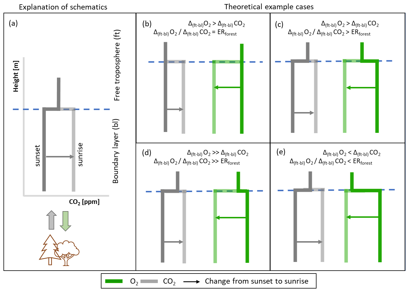
Figure 8Schematic overview of how different ratios of the jumps of O2 (Δ(ft-bl)O2) and CO2 (Δ(ft-bl)CO2) are formed in the nighttime and how the ratio relates to the exchange ratio of the forest (ERforest). Panel (a) gives an explanation of the schematics and the other panels show four possibilities of different jump ratios (Δ(ft-bl)O2 Δ(ft-bl)CO2): (b) the jump ratio is equal to ERforest, (c) the jump ratio is larger than ERforest, (d) the jump ratio is much larger than ERforest, (e) the jump ratio is smaller than ERforest. The bold lines represent the vertical profile just after sunset and the shaded lines represent the vertical profile just before sunrise.
5.3 Different Δ(ft-bl) ratios
Knowing the vertical profile of O2 and CO2, especially during sunrise, is essential to gain a more comprehensive understanding of the formation of different jump ratios (Δ(ft-bl)O2 Δ(ft-bl)CO2) and to better interpret the diurnal behaviour of the ERatmos signal. However, due to a lack of observational data, we cannot validate the vertical profile of O2 and CO2 and the jump ratios. We therefore strongly recommend that future measurement campaigns include vertical measurements of both species. This can, for example, be achieved by flask sampling from aircraft, as we did in a recent campaign in the Netherlands, the preliminary results of which confirm that the values we have used here are realistic. Previous studies have also measured vertical profiles of O2 and CO2, but they primarily focused on well-mixed profiles during daytime or profiles over the ocean (Morgan et al., 2019; Stephens et al., 2021; Ishidoya et al., 2022). Hence, careful consideration of the timing and location of the vertical measurements is important to advance our knowledge of the diurnal behaviour of ERatmos.
In the absence of observational data, we show with hypothetical situations that various jump ratios become possible (Fig. 8). Both the O2 and CO2 jumps are formed as a result of three processes: the mixed-layer value before sunset, the surface flux during the night, and the free troposphere value with the lapse rate (we assume the lapse rate to be 0 mol m−1 for CO2 and O2). Most cases indicate that Δ(ft-bl)O2 is larger than Δ(ft-bl)CO2 above a forest, primarily because ERforest is higher than 1.0 during the night (ERr>1.0), as was shown in previous studies (Ishidoya et al., 2013; Angert et al., 2015; Hilman et al., 2022). It is noteworthy that the movement of the mixed-layer values from sunset to sunrise in Fig. 8 differs from its depiction in Fig. 2c, where the focus was primarily on the transition between sunrise and sunset. We ignore the effect of subsidence (caused by mesoscale or synoptic processes) on the jump evaluation in this analysis, because it is likely of less importance compared to the other three processes.
It is highly likely that the jump ratio between O2 and CO2 cannot be directly linked to a specific ER for a certain process because of the interplay between the three processes that form the O2 and a CO2 jump (Fig. 8d). The likelihood of both Δ(ft-bl)O2 and Δ(ft-bl)CO2 being zero at the end of the day is low, because the surface flux during the day would form a jump (Fig. 8c). Additionally, it is possible that Δ(ft-bl)O2 is smaller than Δ(ft-bl)CO2 at the end of the day (Fig. 8d) due to the daytime ERforest being smaller than 1.0. Consequently, O2 will exhibit a faster movement across the zero line, resulting in a significantly larger Δ(ft-bl)O2 Δ(ft-bl)CO2 ratio compared to ERr.
Decoupling between the free troposphere and the boundary layer can lead to a scenario in which Δ(ft-bl)CO2 becomes larger than Δ(ft-bl)O2 (Fig. 8e). This can occur, for example, when the influence of fossil fuel sources causes a decrease in the O2 mole fraction and an increase in the CO2 mole fraction in the free troposphere, but large surface fluxes from the forest prevent such changes from occurring in the boundary layer. The jump ratio in this case again cannot be attributed to a single process. Some studies have demonstrated that decoupling between the boundary layer and the free troposphere can occur, leading to different ER signals (Sturm et al., 2005; van der Laan et al., 2014).
5.4 Comparison with other studies
To the best of our knowledge, no previous studies have reported such high deviations of ERatmos from ERforest or ERatmos values higher than 2 for above-forest-canopy measurements, as we found in Faassen et al. (2023). Only Liu et al. (2023b) found a non-linear relationship between O2 and other tracers that was difficult to explain. While some differences between ERatmos and ERforest have been observed in previous studies, these differences typically fall within a region of 0.5 (Seibt et al., 2004; Ishidoya et al., 2015; Battle et al., 2019; Yan et al., 2023). A possible reason for these smaller differences could be that most studies do not focus on such detailed diurnal analyses of ERatmos for specific days, but rather aggregate data from multiple days, which could mitigate the extreme effects of entrainment by combining various jump possibilities. However, even in the study by Stephens et al. (2007), in which measurements at different heights are shown, no discernible difference in the ERatmos signal for various diurnal cycles was observed, a finding that contrasts with our own analysis. The height at which measurements are made also influences the resulting ERatmos signal. Closer to the canopy, the influence of entrainment is lower and ERatmos is closer to ERforest compared to measurements further away from the canopy (Faassen et al., 2023). However, we still found a high ERatmos value of 2.28, even at a level just above the canopy (Faassen et al., 2023). Large values for ERatmos have only been found at high-latitude measurement stations (Sturm et al., 2005), due to the influence of the ocean.
There are several possibilities that might explain a constant ERatmos signal during the day which are not shown in our study. One possibility is that entrainment dominates throughout the day, caused by high jumps. If both the O2 and CO2 jumps are extremely high while the surface flux remains low, the ERatmos value reflects the ratios between the jumps. In this scenario, ERatmos cannot be used as an accurate indicator for the surface processes. Another explanation could be that the ERforest signal is exactly 1.0 and entrainment is relatively low. When ERforest equals 1.0, the diurnal cycle of the jumps would respond similarly. Together with a low entrainment flux (resulting from low jumps), it could lead to a constant ERatmos value. Additionally, when the peak of ERatmos occurs rapidly, there is a possibility that a low measurement precision would miss the extreme changes of ERatmos. However, even in such cases, ERatmos would still be influenced by entrainment, although its impact may be less discernible. It is crucial to note that in all these cases, ERatmos remains influenced by entrainment to varying degrees.
Our study provides evidence that ERatmos is almost always influenced by large-scale processes and their diurnal variability, specifically entrainment, making it important to exercise caution when using it as an indicator of surface ER processes. Instances where ERatmos remains constant throughout the daytime and serves as a reliable indication for ERforest are likely rare. In comparison to previous studies (Seibt et al., 2004; Stephens et al., 2007; Ishidoya et al., 2013; Battle et al., 2019), it is unclear why Faassen et al. (2023) yields such extreme values for ERatmos while the other studies do not show this, even though our modelling study here confirms the extreme ERatmos values. Therefore, we recommend conducting more studies or performing detailed analyses of existing O2 and CO2 datasets to gain a better understanding of how changes in ERatmos vary with time and space.
5.5 Comparison with other multi-tracer analyses
The impact of changes in large-scale conditions such as entrainment on multi-tracer analyses above forest canopies extends beyond atmospheric O2, encompassing other carbon cycle tracers such as carbon and oxygen isotopes (δ13C and δ18O) (Wehr et al., 2016) and carbonyl sulfide (COS) (Whelan et al., 2018). Caution is required when employing methods of determining ratios between two species (e.g. leaf relative uptake for COS and the ratios between different isotopes) that rely solely on single-height measurements. However, the influence of entrainment on these ratios would be less extreme compared to that on the ERatmos signal, because both COS and isotopes move in the same direction as CO2 itself. This is differs from the situation with O2, which always moves in the opposite direction to CO2. When both species that form the ratio move in the same direction, ratios of different processes could be averaged and a one-height measurement is more readily interpretable. Nevertheless, entrainment would still cause the two compounds that form the ratio to behave differently. We therefore emphasize the need to separately analyse the composition of the signal for each compound when ratios are analysed.
Furthermore, we demonstrate in this study the potential of using ERatmos as an indicator of the extent of large-scale processes. Additional tracers can strengthen this approach. Also δ13C, δ18O, and COS signals exhibit differences between the surface and the free troposphere. Similar to O2, the onset of entrainment causes these signals to mix, yielding insights into how large-scale processes influence the carbon cycle above a canopy (Berkelhammer et al., 2014; Vilà-Guerau de Arellano et al., 2019). By combining various tracers for CO2, we can create a comprehensive picture of the effects of small- and large-scale processes that influence carbon exchange.
We used a mixed-layer model to analyse the diurnal behaviour of two exchange ratio (ER ) signals above a forest canopy: the ER of the atmosphere (ERatmos, determined from the change over time of O2 and CO2 mole fraction measurements at a single height above the canopy) and the ER of the forest (ERforest, determined from O2 and CO2 fluxes derived from the vertical gradient observations at two levels). We disentangled the biophysical processes influencing ERatmos to interpret single-height O2 and CO2 measurements and to evaluate how ERatmos and ERforest can be used to constrain carbon exchange above the canopy. The analysis is supported by the derivation of a new theoretical relationship that connects ERatmos and ERforest and by the use of a mixed-layer model that reproduces the O2 and CO2 diurnal cycles coupled to the dynamics of the atmospheric boundary layer. By combining the model with observations from a boreal forest during the two contrasting summers of 2018 and 2019, we found three distinct regimes during the day for ERatmos.
We find that the entrainment of air from the free troposphere leads to a diurnal cycle in ERatmos, resulting in three distinctive regimes: P1 at the start of the day, when the boundary layer has not yet started to grow; P2 when entrainment of air from the free troposphere into the boundary layer is dominant; and P3 at the end of the afternoon, when entrainment becomes negligible. ERatmos can exhibit high values during P2 that cannot be attributed to an ER signal from a single process. During P3, ERatmos becomes closer to ERforest, and is therefore more representative of the forest exchange.
The large diurnal variability in ERatmos shows that single-height O2 and CO2 measurements are insufficient as an indication of the O2 CO2 ratios of forest exchange. Our theoretical relationship between ERatmos and ERforest and the model results show that the large diurnal variability is a result of the different behaviours of the O2 and CO2 diurnal cycles, which results in ERatmos values that cannot be attributed to a single process. To estimate the ER signal of the surface fluxes from above-canopy measurements, ERforest should be used and, therefore, O2 and CO2 signals need to be measured at at least two heights to allow fluxes to be calculated from the vertical gradient. A single measurement height for O2 and CO2 could still be used to indicate the presence of advection of other carbon sources. However, the resulting ERatmos signal should be analysed with care, taking into account the diurnal variability and the fact that the resulting ER is not necessarily the average of the individual ER signals of the contributing processes.
When O2 and CO2 measurements are available from two different heights, the relationship between ERatmos and ERforest during P2 and P3 could provide valuable information about the changes in large-scale carbon processes (e.g. entrainment) and their influence on the smaller-scale processes of the surface. A discrepancy between ERatmos and ERforest shows that large-scale processes occur together with small-scale processes at the surface. The difference between ERatmos and ERforest should be analysed with care, as the size of the difference is not a direct indication of the size of the influence of the large-scale processes. Differences between ERforest and ERatmos could be caused by several factors: changes in the size of the entrainment flux, the net surface flux or the difference between the free troposphere and the boundary layer (the “jump”) for O2 and/or CO2, or changes in the jump ratio between O2 and CO2.
In conclusion, single-height O2 and CO2 measurements need to be analysed with care, accounting for their dependence on canopy processes (represented by ERforest) but also for their capacity to integrate large-scale processes, resulting in values that cannot be attributed to a single process. To represent the forest exchange, the ERforest signal based on measurements at at least two heights should be used instead.
A1 Evaluation of the theoretical relationship between ERatmos and ERforest
In this section, we analyse Eq. (8) to explore the response of ERatmos to changes in the variables in this equation and to investigate when ERatmos aligns with ERforest and thereby accurately reflects local processes. Based on Eq. (8), the ERatmos signal equals ERforest when the β values of O2 and CO2 are equal. We can define four different regimes where the β values change significantly. As depicted in Fig. 1, we can define two regimes based on the entrainment velocity: an entrainment-driven (left panels in Fig. A1) and a photosynthesis-driven regime (right panels in Fig. A1). To complete the analysis, we considered two distinct cases for the jump of O2 (top versus bottom panels).
Based on Eq. (8), we systematically varied Δ(ft-bl)CO2 and over plausible ranges and kept the other variables constant. As a result, we derived ERforest ERatmos ratios for these four regimes, where a value of 1.0 now indicates that ERatmos is equal to ERforest. The selected values and ranges for the four different cases were informed by initial conditions from the Hyytiälä case studied in Faassen et al. (2023) and the corresponding model simulations presented in Sect. 3.2.4.
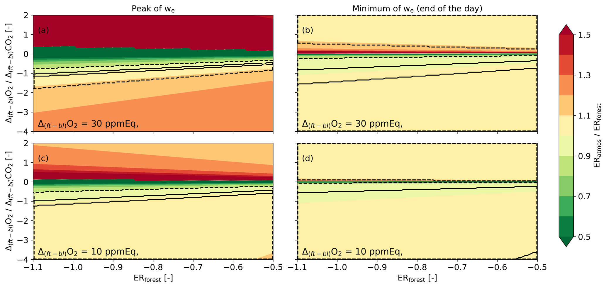
Figure A1Analysis of Eq. (8) for the entrainment- and photosynthesis-driven regimes. The ratio between ERforest and ERatmos is evaluated based on changes in ERforest and the ratio of the jumps of O2 and CO2 between the free troposphere and the boundary layer (Δ(ft-bl)) for four cases: with a high entrainment velocity (we=0.10 m s−1) (a, c) and a low entrainment velocity (we=0.01 m s−1) (b, d), and for situations with a high O2 jump (Δ(ft-bl)O2=0.30 ppmEq) (a, b) and a low O2 jump (Δ(ft-bl)O2=0.10 ppmEq) (c, d). The O2 surface flux F(O2)s is kept constant for all the panels at 8.5 µmol m s−1.
There are a few situations where the β values of O2 and CO2 are equal and these are indicated in Fig. A1 as the area between the black solid (ERatmos deviates <1 % from ERforest) and dashed lines (ERatmos deviates <10 % from ERforest):
-
During the photosynthesis dominant regime. When the entrainment velocity (we) is close to zero, both β values become zero. This is likely at the end of the day (right panels in Fig. 1).
-
When the β values for O2 and CO2 become equal, which happens when Δ(ft-bl)O2 Δ(ft-bl)CO2 = ERforest. A specific case is when Δ(ft-bl)O2 = Δ(ft-bl)CO2. In this instance, ERforest has to be 1.0 for the β values of O2 and CO2 to become equal. The β values of O2 and CO2 become closer during the lower O2 jump case (lower panels in Fig. 1).
The last situation only occurs under very specific conditions when the ratio of the O2 and CO2 entrainment and surface fluxes are the same. This is visible in the left panels of Fig. A1, where only a small part of the graph shows values of ERatmos close to ERforest (indicated by the area between the solid lines). In contrast, during low entrainment velocities at the end of the afternoon, it is more likely that the ERatmos values become close to ERforest, and this is shown by the larger area in the right panels of Fig. A1. Low entrainment velocities could also occur when the growth of the boundary layer is reduced due to subsidence, although we do not focus on this specific case in this study.
There are also differences between ERatmos and ERforest that arise from variations in the β values. Figure A1 demonstrates that substantial differences between ERatmos and ERforest originate due to differences in the entrainment fluxes of both species. When Δ(ft-bl)O2 exceeds Δ(ft-bl)CO2, this implies a dominant entrainment flux of O2 over CO2 and deviates further from (Eq. 8). This effect is almost absent when the jumps themselves are lower, because the ERatmos/ERforest ratio stays around 1 (Fig. A1c). Moreover, when Δ(ft-bl)CO2 transitions from negative to positive, the sign of also changes, subsequently elevating the ERatmos values (Eq. 8).
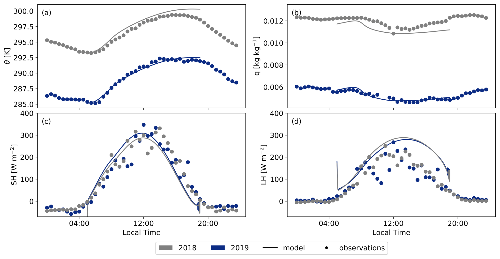
Figure A2Comparison between the 2019 and 2018 cases modelled with CLASS with the observational data for the potential temperature (θ) (a), specific humidity (q) (b), sensible heat flux (SH) (c), and latent heat flux (LH) (d).
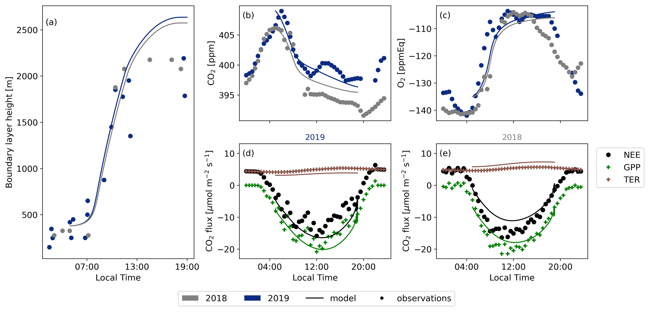
Figure A3Comparison between the 2019 and 2018 cases modelled with CLASS using the observational data for the boundary layer height (a), CO2 (b), O2 (c), the 2019 CO2 surface fluxes (d), and the 2018 CO2 surface fluxes (e).
ERatmos can also become smaller than ERforest when Δ(ft-bl)CO2 is larger than Δ(ft-bl)O2 (Fig. A1). This difference results in a large value for compared to , causing the ERforest value to be multiplied by a factor of less than 1 and leading to a lower ERatmos value than ERforest (Eq. 8). By assessing ERatmos and ERforest values, we can see whether Δ(ft-bl)O2 exceeds Δ(ft-bl)CO2 (ERatmos> ERforest) or vice versa (ERatmos< ERforest).
This illustrative analysis, based on prescribed values in Eq. (8) and Fig. A1, provides an initial estimate of the variability in ERatmos. However, it lacks insights into the diurnal behaviour of the individual components of Eq. (8) and their potential combinations.
A2 Implementation of O2 in CLASS
The following equation shows the implementation of the tendency (change over time) of O2 into CLASS:
where is the net surface O2 flux at the canopy, is the O2 entrainment flux, h is the boundary layer height, and adv is the advection term. The surface flux is calculated with Eq. (10) and the entrainment flux is based on the following equation (see also Eq. 2):
where we is the entrainment velocity and Δ(ft-bl)O2 is the jump of O2. The jump of O2 was determined the same way as for CO2, by tuning the initialization of the jump until the decrease or increase of CO2 O2 of the model matched with the observational data.
A3 Validation of CLASS
Figures A3 and A2 present a comparison between the model output of CLASS and the corresponding measurements for the representative days of 2018 and 2019, assessing various parameters. Both figures demonstrate that the model compares well to the observed data. CLASS accurately follows the observed temperature increase (Fig. A2a). A constant difference of approximately 8K between 2018 and 2019 is seen for both the model and the observations. This persistent difference is attributed to a heat wave rather than a drought in Hyytiälä, as a drought would have intensified the divergence between the 2018 and 2019 simulations throughout the day. Moreover, CLASS adequately models specific humidity for both years, assuming an initial relative humidity of 80 % for 2018 (Fig. A2b). The sensible heat flux (Fig. A2c) and latent heat flux (Fig. A2d) exhibit minimal differences between the 2018 and 2019 simulations. The accurate representation of atmospheric properties in CLASS consequently results in a satisfactory representation of boundary layer height development for both years in comparison to the observed data from radiosondes (Fig. A3a)
The various CO2 fluxes simulated by CLASS exhibit a high level of agreement with the observational data for both 2018 and 2019 (Fig. A3d and e). While there are subtle differences evident between the observations for the two years, CLASS adeptly captures these nuances. Consequently, the model provides an accurate representation of plant behaviour under both normal and warmer conditions. The elevated temperatures (+8 K) and slightly reduced soil moisture (−0.03 m3 m−3) contribute to a slightly higher GPP and TER flux. Our study reaffirms that the vegetation in Hyytiälä did not undergo any stress during the 2018 European drought, which would have resulted in a lower GPP and lower latent heat flux (Lindroth et al., 2020).
For the 2018 case, we altered only a few initial conditions (see Table C3). However, both the decrease in CO2 and the increase in O2 during the day exhibit close similarity between the model and the observations. This outcome underscores that even with minimal changes in the initial conditions for the 2018 case and while keeping the other variables constant (e.g. the jumps), we can successfully replicate a realistic new day based on the base case.
It is important to note that only the net ecosystem exchange (NEE) data are obtained directly from eddy covariance measurements. The gross primary production (GPP) is inferred from a light- and temperature-based function and the total ecosystem respiration is calculated as the residual between NEE and GPP (Kulmala et al., 2019; Kohonen et al., 2022). This distinction may explain the challenge in aligning the TER flux of the observations with the model, as the model exhibits notable discrepancies from the observations for the 2018 and 2019 cases. The model's simulated respiration increase based on temperature appears more extreme compared to the observations. However, several studies (Lindroth et al., 2008; Gao et al., 2017; Heiskanen et al., 2023) indicate that the model's increase in TER between 2018 and 2019 is slightly too high, while the change based on observations is too low. As a result, it is plausible that the true respiration flux lies somewhere between the model output and the observational data.
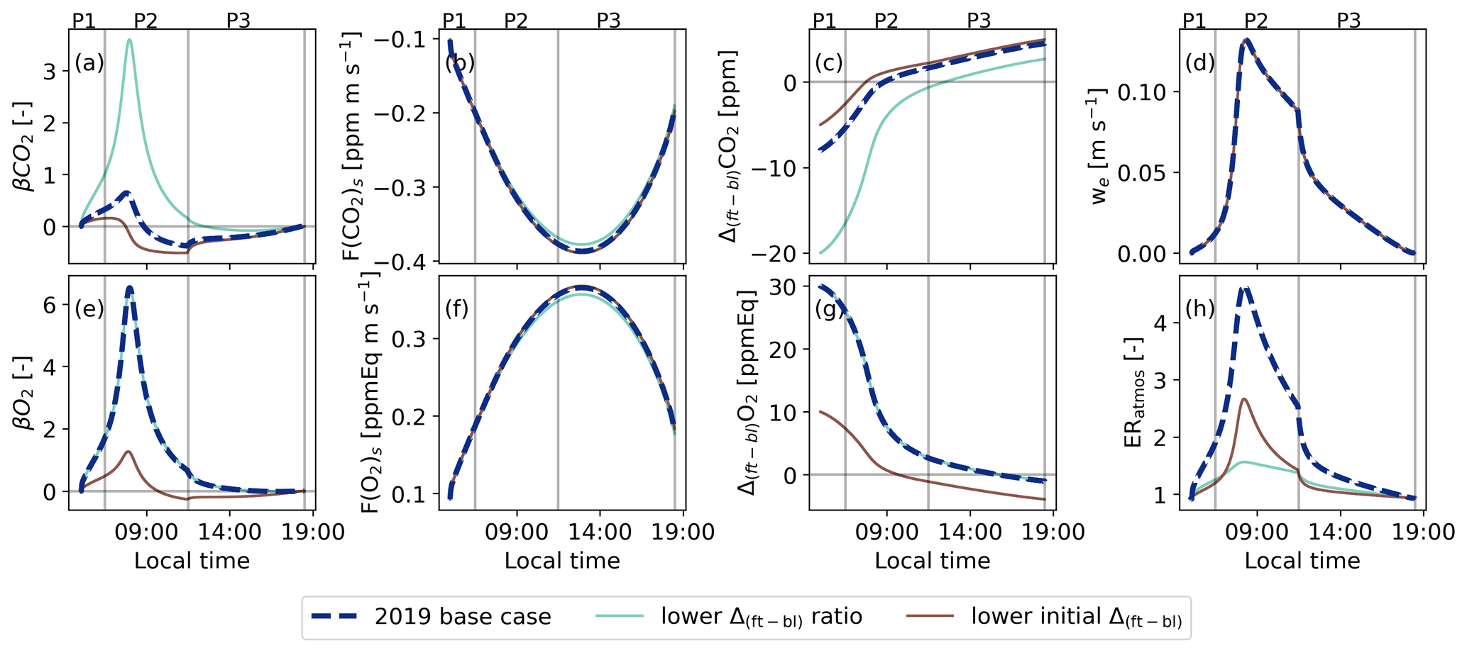
Figure B1Similar to Fig. 5 but now for the base case (2019) and the background sensitivity studies with a lower jump ratio between O2 and CO2 (lower Δ(ft-bl)), and with a lower initial jump for CO2 (lower initial Δ(ft-bl)). The diurnal variability of the exchange ratio of the atmosphere is now added (ERatmos: (h)).
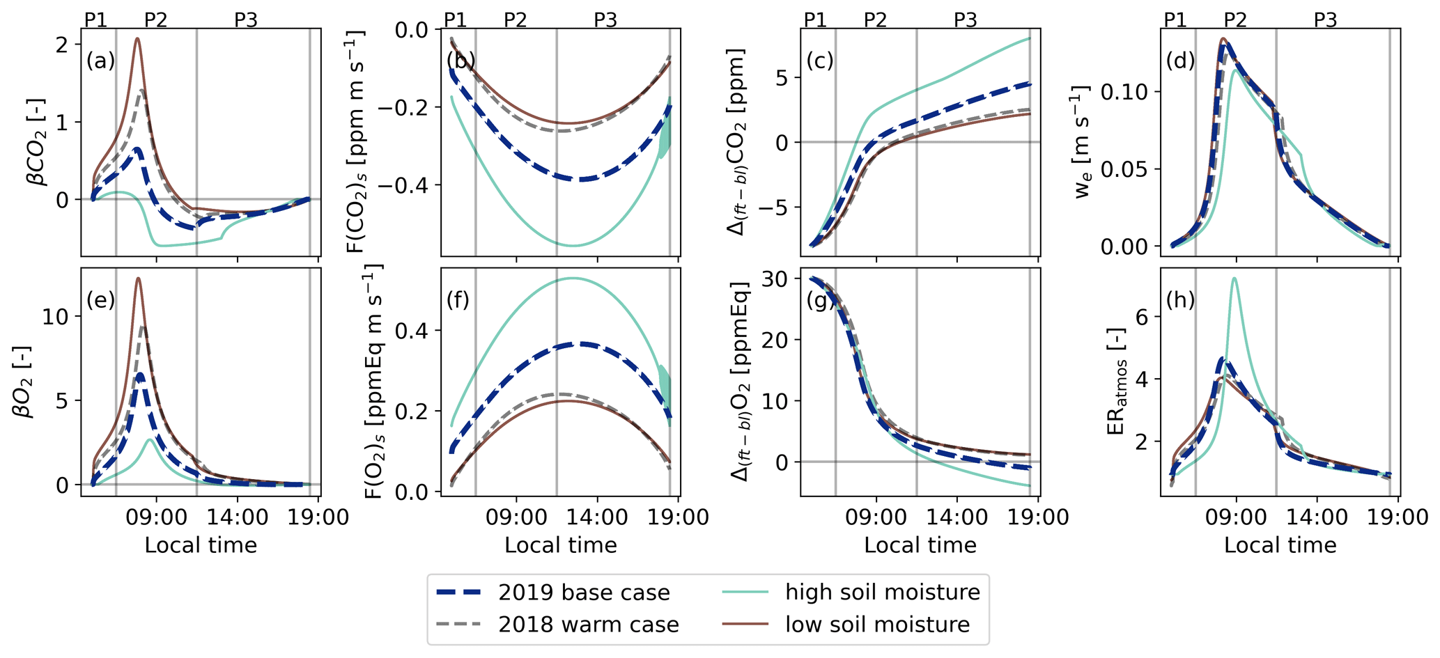
Figure B2Similar to Fig. 5 but now for the base case (2019) and the dry and warm sensitivity studies with a high soil moisture and a low soil moisture, both with higher air temperatures compared to the 2019 base case. The diurnal variability of the exchange ratio of the atmosphere is now added (ERatmos: (h)).
Table C1The initial conditions used for the three sensitivity analyses compared to the initial conditions for the 2019 base case. The subscript (0) indicates the first time step.
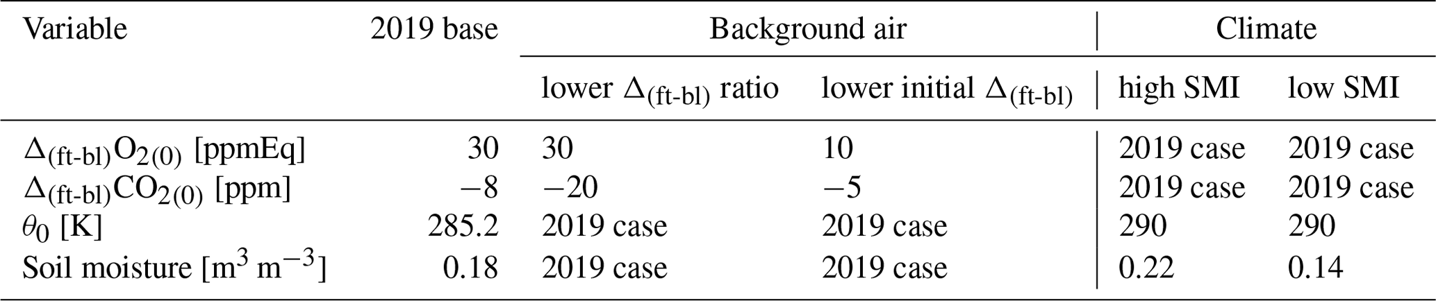
Table C2Initialization of the CLASS model for the 2019 base case based on 10 July 2019. The initialization is based on the SMEAR II data (Hari et al., 2013), our OXHYYGEN campaign data (radiosondes or O2 and CO2 measurements) (Faassen et al., 2023), and studies that show ranges for parameters for the plants and soil (Lindroth et al., 2008; ECMWF IV, 2014; Vilà-Guerau de Arellano et al., 2015).
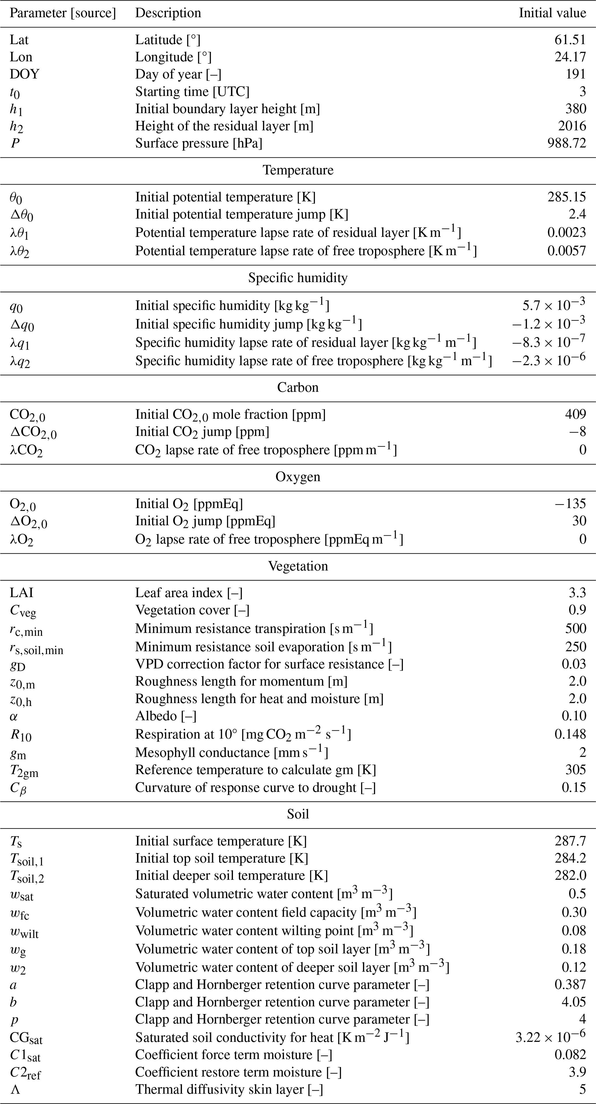
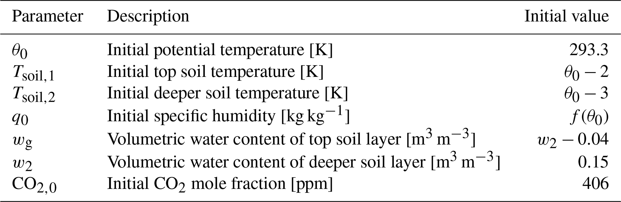
Table C3Adjustments for the 2018 case (warm case) compared to the 2019 values shown in Table C2. Only the initial potential temperature (θ0), initial soil moisture (wg), and CO2 mole fraction (CO2,0) are adjusted based on the aggregate of 28 and 29 July 2018. It was assumed that the initial relative humidity stayed constant at 80 % with increasing temperatures; therefore, the initial specific humidity was also adjusted.
The data used in this study are available from https://doi.org/10.18160/SJ3J-PD38 (Faassen and Luijkx, 2022). The model code for the CLASS model can be found in https://classmodel.github.io/ (Vilà-Guerau de Arellano et al., 2015).
KAPF, JVGdA, ITL, and RGA set up the model analysis. KAPF, ITL, JVGdA, and WP interpreted and discussed the methods and results. ITL designed the measurement campaign and conducted the O2 and CO2 measurements, and BGH conducted the radiosonde measurements with input from JVGdA and support from IM. KAPF and ITL wrote the manuscript with input from all co-authors.
The contact author has declared that none of the authors has any competing interests.
Publisher’s note: Copernicus Publications remains neutral with regard to jurisdictional claims made in the text, published maps, institutional affiliations, or any other geographical representation in this paper. While Copernicus Publications makes every effort to include appropriate place names, the final responsibility lies with the authors.
The authors would like to thank the following persons for their help during the measurement campaigns at Hyytiälä in 2018 and 2019: Janne Levula (previously at the Institute for Atmospheric and Earth System Research (INAR)/Physics, Faculty of Science, University of Helsinki, Helsinki, Finland), Timo Vesala (Institute for Atmospheric and Earth System Research (INAR)/Physics, Faculty of Science, University of Helsinki, Helsinki, Finland), Linh N. T. Nguyen (previously at the University of Groningen, Centre for Isotope Research, Energy and Sustainability Research Institute Groningen, Groningen, the Netherlands), Bert Kers (University of Groningen, Centre for Isotope Research, Energy and Sustainability Research Institute Groningen, Groningen, the Netherlands), and Brian Verhoeven (former student at Meteorology and Air Quality, Wageningen University, Wageningen, the Netherlands). We acknowledge Ruben van't Loo (student at Meteorology and Air Quality, Wageningen University, Wageningen, the Netherlands) for his contribution to the data analysis. We have used ChatGPT as a language editor to improve the readability of certain parts of an earlier version of the paper.
This research has been supported by the Aard- en Levenswetenschappen, Nederlandse Organisatie voor Wetenschappelijk Onderzoek (grant nos. VI.Vidi.213.143 and 016.Veni.171.095); the Netherlands Organisation for Scientific Research for ITL (grant nos. 016.Veni.171.095 and VI.Vidi.213.143); and the University of Helsinki via ICOS-HY funding and the GreenFeedBack project from the EU Horizon Europe – Framework Programme for Research and Innovation (grant no. 101056921).
This paper was edited by Paul Stoy and reviewed by two anonymous referees.
Angert, A., Yakir, D., Rodeghiero, M., Preisler, Y., Davidson, E. A., and Weiner, T.: Using O2 to study the relationships between soil CO2 efflux and soil respiration, Biogeosciences, 12, 2089–2099, https://doi.org/10.5194/bg-12-2089-2015, 2015. a, b, c, d
Battle, M. O., Munger, J. W., Conley, M., Sofen, E., Perry, R., Hart, R., Davis, Z., Scheckman, J., Woogerd, J., Graeter, K., Seekins, S., David, S., and Carpenter, J.: Atmospheric measurements of the terrestrial O2 : CO2 exchange ratio of a midlatitude forest, Atmos. Chem. Phys., 19, 8687–8701, https://doi.org/10.5194/acp-19-8687-2019, 2019. a, b, c, d
Berkelhammer, M., Asaf, D., Still, C., Montzka, S., Noone, D., Gupta, M., Provencal, R., Chen, H., and Yakir, D.: Constraining surface carbon fluxes using in situ measurements of carbonyl sulfide and carbon dioxide, Global Biogeochem. Cy., 28, 161–179, 2014. a
Bloom, A. J.: Photorespiration and nitrate assimilation: a major intersection between plant carbon and nitrogen, Photosynth. Res., 123, 117–128, 2015. a, b, c
Casso-Torralba, P., Vilà-Guerau de Arellano, J., Bosveld, F., Soler, M. R., Vermeulen, A., Werner, C., and Moors, E.: Diurnal and vertical variability of the sensible heat and carbon dioxide budgets in the atmospheric surface layer, J. Geophys. Res.-Atmos., 113, https://doi.org/10.1029/2007JD009583, 2008. a, b
Combe, M., Vilà-Guerau de Arellano, J., Ouwersloot, H. G., Jacobs, C. M. J., and Peters, W.: Two perspectives on the coupled carbon, water and energy exchange in the planetary boundary layer, Biogeosciences, 12, 103–123, https://doi.org/10.5194/bg-12-103-2015, 2015. a
ECMWF IV, I.: Documentation–Cy40r1 Part IV: Physical Processes, European Centre for Medium-Range Weather Forecasts: Reading, UK, 111–113, 2014. a, b
Faassen, K. and Luijkx, I.: Atmospheric O2 and CO2 measurements at Hyytiälä, Finland, ICOS carbon portal [data set], https://doi.org/10.18160/SJ3J-PD38, 2022. a
Faassen, K. A. P., Nguyen, L. N. T., Broekema, E. R., Kers, B. A. M., Mammarella, I., Vesala, T., Pickers, P. A., Manning, A. C., Vilà-Guerau de Arellano, J., Meijer, H. A. J., Peters, W., and Luijkx, I. T.: Diurnal variability of atmospheric O2, CO2, and their exchange ratio above a boreal forest in southern Finland, Atmos. Chem. Phys., 23, 851–876, https://doi.org/10.5194/acp-23-851-2023, 2023. a, b, c, d, e, f, g, h, i, j, k, l, m, n, o, p, q, r, s, t, u, v, w, x
Fischer, S., Hanf, S., Frosch, T., Gleixner, G., Popp, J., Trumbore, S., and Hartmann, H.: Pinus sylvestris switches respiration substrates under shading but not during drought, New Phytol., 207, 542–550, 2015. a, b
Friedlingstein, P., Jones, M. W., O'Sullivan, M., Andrew, R. M., Bakker, D. C. E., Hauck, J., Le Quéré, C., Peters, G. P., Peters, W., Pongratz, J., Sitch, S., Canadell, J. G., Ciais, P., Jackson, R. B., Alin, S. R., Anthoni, P., Bates, N. R., Becker, M., Bellouin, N., Bopp, L., Chau, T. T. T., Chevallier, F., Chini, L. P., Cronin, M., Currie, K. I., Decharme, B., Djeutchouang, L. M., Dou, X., Evans, W., Feely, R. A., Feng, L., Gasser, T., Gilfillan, D., Gkritzalis, T., Grassi, G., Gregor, L., Gruber, N., Gürses, Ö., Harris, I., Houghton, R. A., Hurtt, G. C., Iida, Y., Ilyina, T., Luijkx, I. T., Jain, A., Jones, S. D., Kato, E., Kennedy, D., Klein Goldewijk, K., Knauer, J., Korsbakken, J. I., Körtzinger, A., Landschützer, P., Lauvset, S. K., Lefèvre, N., Lienert, S., Liu, J., Marland, G., McGuire, P. C., Melton, J. R., Munro, D. R., Nabel, J. E. M. S., Nakaoka, S.-I., Niwa, Y., Ono, T., Pierrot, D., Poulter, B., Rehder, G., Resplandy, L., Robertson, E., Rödenbeck, C., Rosan, T. M., Schwinger, J., Schwingshackl, C., Séférian, R., Sutton, A. J., Sweeney, C., Tanhua, T., Tans, P. P., Tian, H., Tilbrook, B., Tubiello, F., van der Werf, G. R., Vuichard, N., Wada, C., Wanninkhof, R., Watson, A. J., Willis, D., Wiltshire, A. J., Yuan, W., Yue, C., Yue, X., Zaehle, S., and Zeng, J.: Global Carbon Budget 2021, Earth Syst. Sci. Data, 14, 1917–2005, https://doi.org/10.5194/essd-14-1917-2022, 2022. a
Gao, Y., Markkanen, T., Aurela, M., Mammarella, I., Thum, T., Tsuruta, A., Yang, H., and Aalto, T.: Response of water use efficiency to summer drought in a boreal Scots pine forest in Finland, Biogeosciences, 14, 4409–4422, https://doi.org/10.5194/bg-14-4409-2017, 2017. a, b
Gibelin, A.-L., Calvet, J.-C., and Viovy, N.: Modelling energy and CO2 fluxes with an interactive vegetation land surface model-Evaluation at high and middle latitudes, Agr. Forest Meteorol., 148, 1611–1628, 2008. a
Hari, P., Nikinmaa, E., Pohja, T., Siivola, E., Bäck, J., Vesala, T., and Kulmala, M.: Station for measuring ecosystem-atmosphere relations: SMEAR, in: Physical and physiological forest ecology, 471–487, Springer, https://doi.org/10.1007/978-94-007-5603-8_9, 2013. a, b, c
Heiskanen, L., Tuovinen, J.-P., Vekuri, H., Räsänen, A., Virtanen, T., Juutinen, S., Lohila, A., Mikola, J., and Aurela, M.: Meteorological responses of carbon dioxide and methane fluxes in the terrestrial and aquatic ecosystems of a subarctic landscape, Biogeosciences, 20, 545–572, https://doi.org/10.5194/bg-20-545-2023, 2023. a
Hilman, B. and Angert, A.: Measuring the ratio of CO2 efflux to O2 influx in tree stem respiration, Tree Physiol., 36, 1422–1431, 2016. a
Hilman, B., Weiner, T., Haran, T., Masiello, C. A., Gao, X., and Angert, A.: The apparent respiratory quotient of soils and tree stems and the processes that control it, J. Geophys. Res.-Biogeo., 127, e2021JG006676, https://doi.org/10.1029/2021JG006676, 2022. a, b, c, d, e
Ishidoya, S., Murayama, S., Takamura, C., Kondo, H., Saigusa, N., Goto, D., Morimoto, S., Aoki, N., Aoki, S., and Nakazawa, T.: O2:CO2 exchange ratios observed in a cool temperate deciduous forest ecosystem of central Japan, Tellus B, 65, 21120, https://doi.org/10.3402/tellusb.v65i0.21120, 2013. a, b, c, d, e, f
Ishidoya, S., Murayama, S., Kondo, H., Saigusa, N., Kishimoto-Mo, A. W., and Yamamoto, S.: Observation of O2:CO2 exchange ratio for net turbulent fluxes and its application to forest carbon cycles, Ecol. Res., 30, 225–234, https://doi.org/10.1007/s11284-014-1241-3, 2015. a, b, c, d
Ishidoya, S., Sugawara, H., Terao, Y., Kaneyasu, N., Aoki, N., Tsuboi, K., and Kondo, H.: O2 : CO2 exchange ratio for net turbulent flux observed in an urban area of Tokyo, Japan, and its application to an evaluation of anthropogenic CO2 emissions, Atmos. Chem. Phys., 20, 5293–5308, https://doi.org/10.5194/acp-20-5293-2020, 2020. a, b
Ishidoya, S., Tsuboi, K., Niwa, Y., Matsueda, H., Murayama, S., Ishijima, K., and Saito, K.: Spatiotemporal variations of the δ(O2/N2), CO2 and δ(APO) in the troposphere over the western North Pacific, Atmos. Chem. Phys., 22, 6953–6970, https://doi.org/10.5194/acp-22-6953-2022, 2022. a
Ishidoya, S., Tsuboi, K., Kondo, H., Ishijima, K., Aoki, N., Matsueda, H., and Saito, K.: Measurement report: Method for evaluating CO2 emissions from a cement plant using atmospheric δ(O2/N2) and CO2 measurements and its implication for future detection of CO2 capture signals, Atmos. Chem. Phys., 24, 1059–1077, https://doi.org/10.5194/acp-24-1059-2024, 2024. a
Jacobs, C., Van den Hurk, B., and De Bruin, H.: Stomatal behaviour and photosynthetic rate of unstressed grapevines in semi-arid conditions, Agr. Forest Meteorol., 80, 111–134, 1996. a, b, c
Kaimal, J. C. and Finnigan, J. J.: Atmospheric boundary layer flows: their structure and measurement, Oxford University Press, https://doi.org/10.1093/oso/9780195062397.001.0001, 1994. a
Keeling, R. F. and Manning, A. C.: Studies of Recent Changes in Atmospheric O2 Content, vol. 5, Elsevier Ltd., 2 edn., ISBN 9780080983004, https://doi.org/10.1016/B978-0-08-095975-7.00420-4, 2014. a
Keeling, R. F., Manning, A. C., McEvoy, E. M., and Shertz, S. R.: Methods for measuring changes in atmospheric O2 concentration and their application in southern hemisphere air, J. Geophys. Res.-Atmos., 103, 3381–3397, 1998. a, b
Kohonen, K.-M., Dewar, R., Tramontana, G., Mauranen, A., Kolari, P., Kooijmans, L. M. J., Papale, D., Vesala, T., and Mammarella, I.: Intercomparison of methods to estimate gross primary production based on CO2 and COS flux measurements, Biogeosciences, 19, 4067–4088, https://doi.org/10.5194/bg-19-4067-2022, 2022. a
Kulmala, L., Pumpanen, J., Kolari, P., Dengel, S., Berninger, F., Köster, K., Matkala, L., Vanhatalo, A., Vesala, T., and Bäck, J.: Inter-and intra-annual dynamics of photosynthesis differ between forest floor vegetation and tree canopy in a subarctic Scots pine stand, Agr. Forest Meteorol., 271, 1–11, 2019. a
Lilly, D. K.: Models of cloud-topped mixed layers under a strong inversion, Q. J. Roy. Meteor. Soc., 94, 292–309, 1968. a
Lindroth, A., Lagergren, F., Aurela, M., Bjarnadottir, B., Christensen, T., Dellwik, E., Grelle, A., Ibrom, A., Johansson, T., Lankreijer, H., Launiainen, S., Laurila, T., Mölder, M., Nikinmaa, E., Pilegaard, K., Sigurdsson, B. D., and Vesala, T.: Leaf area index is the principal scaling parameter for both gross photosynthesis and ecosystem respiration of Northern deciduous and coniferous forests, Tellus B, 60, 129–142, 2008. a, b
Lindroth, A., Holst, J., Linderson, M.-L., Aurela, M., Biermann, T., Heliasz, M., Chi, J., Ibrom, A., Kolari, P., Klemedtsson, L., Krasnova, A., Laurila, T., Lehner, I., Lohila, A., Mammarella, I., Mölder, M., Löfvenius, M. O., Peichl, M., Pilegaard, K., Soosaar, K., Vesala, T., Vestin, P., Weslien, P., and Nilsson, M.: Effects of drought and meteorological forcing on carbon and water fluxes in Nordic forests during the dry summer of 2018, Philos. T. Roy. Soc. B, 375, 20190516, https://doi.org/10.1098/rstb.2019.0516, 2020. a, b, c
Liu, X., Huang, J., Wang, L., Lian, X., Li, C., Ding, L., Wei, Y., Chen, S., Wang, Y., Li, S., and Shi, J.: “Urban Respiration” Revealed by Atmospheric O2 Measurements in an Industrial Metropolis, Environ. Sci. Technol., 57, 2286–2296, https://doi.org/10.1021/acs.est.2c07583, 2023a. a
Liu, X., Wang, L., Huang, J., Wang, Y., Li, C., Ding, L., Lian, X., and Shi, J.: Revealing the Covariation of Atmospheric O2 and Pollutants in an Industrial Metropolis by Explainable Machine Learning, Environ. Sci. Tech. Lett., 2023b. a
Manning, A. C. and Keeling, R. F.: Global oceanic and land biotic carbon sinks from the scripps atmospheric oxygen flask sampling network, Tellus B, 58, 95–116, https://doi.org/10.1111/j.1600-0889.2006.00175.x, 2006. a
Miller, J. B. and Tans, P. P.: Calculating isotopic fractionation from atmospheric measurements at various scales, Tellus B, 55, 207–214, 2003. a
Morgan, E. J., Stephens, B. B., Long, M. C., Keeling, R. F., Bent, J. D., McKain, K., Sweeney, C., Hoecker-Martínez, M. S., and Kort, E. A.: Summertime Atmospheric Boundary Layer Gradients of O2 and CO2 over the Southern Ocean, J. Geophys. Res.-Atmos., 124, 13439–13456, 2019. a
Ouwersloot, H. G., Vilà-Guerau de Arellano, J., Nölscher, A. C., Krol, M. C., Ganzeveld, L. N., Breitenberger, C., Mammarella, I., Williams, J., and Lelieveld, J.: Characterization of a boreal convective boundary layer and its impact on atmospheric chemistry during HUMPPA-COPEC-2010, Atmos. Chem. Phys., 12, 9335–9353, https://doi.org/10.5194/acp-12-9335-2012, 2012. a
Peters, W., Bastos, A., Ciais, P., and Vermeulen, A.: A historical, geographical and ecological perspective on the 2018 European summer drought, Philos. T. Roy. Soc. B, 375, 20190505, https://doi.org/10.1098/rstb.2019.0505, 2020. a
Pickers, P. A., Manning, A. C., Le Quéré, C., Forster, G. L., Luijkx, I. T., Gerbig, C., Fleming, L. S., and Sturges, W. T.: Novel quantification of regional fossil fuel CO2 reductions during COVID-19 lockdowns using atmospheric oxygen measurements, Sci. Adv., 8, eabl9250, https://doi.org/10.1126/sciadv.abl9250, 2022. a
Reichstein, M., Falge, E., Baldocchi, D., Papale, D., Aubinet, M., Berbigier, P., Bernhofer, C., Buchmann, N., Gilmanov, T., Granier, A., Grunwald, T., Havrankova, K., Ilvesniemi, H., Janous, D., Knohl, A., Laurila, T., Lohila, A., Loustau, D., Matteucci, G., Meyers, T., Miglietta, F., Ourcival, J. M., Pumpanen, J., Rambal, S., Rotenberg, E., Sanz, M., Tenhunen, J., Seufert, G., Vaccari, F., Vesala, T., Yakir, D., and Valentini, R.: On the separation of net ecosystem exchange into assimilation and ecosystem respiration: review and improved algorithm, Glob. Change Biol., 11, 1424–1439, 2005. a
Rödenbeck, C., Le Quéré, C., Heimann, M., and Keeling, R. F.: Interannual variability in oceanic biogeochemical processes inferred by inversion of atmospheric O2/N2 and CO2 data, Tellus B, 60 B, 685–705, https://doi.org/10.1111/j.1600-0889.2008.00375.x, 2008. a
Rödenbeck, C., Adcock, K. E., Eritt, M., Gachkivskyi, M., Gerbig, C., Hammer, S., Jordan, A., Keeling, R. F., Levin, I., Maier, F., Manning, A. C., Moossen, H., Munassar, S., Pickers, P. A., Rothe, M., Tohjima, Y., and Zaehle, S.: The suitability of atmospheric oxygen measurements to constrain western European fossil-fuel CO2 emissions and their trends, Atmos. Chem. Phys., 23, 15767–15782, https://doi.org/10.5194/acp-23-15767-2023, 2023. a
Ronda, R., De Bruin, H., and Holtslag, A.: Representation of the canopy conductance in modeling the surface energy budget for low vegetation, J. Appl. Meteorol. Clim., 40, 1431–1444, 2001. a, b
Schulte, R., van Zanten, M., Rutledge-Jonker, S., Swart, D., Kruit, R. W., Krol, M., van Pul, W., and de Arellano, J. V.-G.: Unraveling the diurnal atmospheric ammonia budget of a prototypical convective boundary layer, Atmos. Environ., 249, 118153, https://doi.org/10.1016/j.atmosenv.2020.118153, 2021. a
Seibt, U., Brand, W. A., Heimann, M., Lloyd, J., Severinghaus, J. P., and Wingate, L.: Observations of O2 : CO2 exchange ratios during ecosystem gas exchange, Global Biogeochem. Cy., 18, 1–18, https://doi.org/10.1029/2004GB002242, 2004. a, b, c, d, e, f
Severinghaus, J. P.: Studies of the Terrestrial O2 and Carbon Cycles in Sand Dune Gases and in Biosphere, PhD thesis, Columbia University, https://doi.org/10.2172/477735, 1995. a, b, c
Stephens, B. B., Keeling, R. F., Heimann, M., Six, K. D., Murnane, R., and Caldeira, K.: Testing global ocean carbon cycle models using measurements of atmospheric O2 and CO2 concentration, Global Biogeochem. Cy., 12, 213–230, https://doi.org/10.1029/97GB03500, 1998. a
Stephens, B. B., Bakwin, P. S., Tans, P. P., Teclaw, R. M., and Baumann, D. D.: Application of a differential fuel-cell analyzer for measuring atmospheric oxygen variations, J. Atmos. Ocean. Tech., 24, 82–94, 2007. a, b
Stephens, B. B., Morgan, E. J., Bent, J. D., Keeling, R. F., Watt, A. S., Shertz, S. R., and Daube, B. C.: Airborne measurements of oxygen concentration from the surface to the lower stratosphere and pole to pole, Atmos. Meas. Tech., 14, 2543–2574, https://doi.org/10.5194/amt-14-2543-2021, 2021. a
Sturm, P., Leuenberger, M., and Schmidt, M.: Atmospheric O2, CO2 and δ13C observations from the remote sites Jungfraujoch, Switzerland, and Puy de Dôme, France, Geophys. Res. Lett., 32, https://doi.org/10.1029/2005GL023304, 2005. a, b
Tennekes, H.: A model for the dynamics of the inversion above a convective boundary layer, J. Atmos. Sci., 30, 558–567, 1973. a
Tohjima, Y., Mukai, H., Machida, T., Hoshina, Y., and Nakaoka, S.-I.: Global carbon budgets estimated from atmospheric O2/N2 and CO2 observations in the western Pacific region over a 15-year period, Atmos. Chem. Phys., 19, 9269–9285, https://doi.org/10.5194/acp-19-9269-2019, 2019. a
van der Laan, S., Van der Laan-Luijkx, I., Rödenbeck, C., Varlagin, A., Shironya, I., Neubert, R., Ramonet, M., and Meijer, H.: Atmospheric CO2, δ (O2/N2), APO and oxidative ratios from aircraft flask samples over Fyodorovskoye, Western Russia, Atmos. Environ., 97, 174–181, 2014. a
van Heerwaarden, C. C. and Teuling, A. J.: Disentangling the response of forest and grassland energy exchange to heatwaves under idealized land–atmosphere coupling, Biogeosciences, 11, 6159–6171, https://doi.org/10.5194/bg-11-6159-2014, 2014. a
Vilà-Guerau de Arellano, J., Gioli, B., Miglietta, F., Jonker, H. J., Baltink, H. K., Hutjes, R. W., and Holtslag, A. A.: Entrainment process of carbon dioxide in the atmospheric boundary layer, J. Geophys. Res.-Atmos., 109, https://doi.org/10.1029/2004JD004725, 2004. a, b
Vilà-Guerau de Arellano, J., Van Heerwaarden, C. C., and Lelieveld, J.: Modelled suppression of boundary-layer clouds by plants in a CO2-rich atmosphere, Nat. Geosci., 5, 701–704, 2012. a, b, c
Vilà-Guerau de Arellano, J., van Heerwaarden, C. C., van Stratum, B. J., and van den Dries, K.: Atmospheric boundary layer: Integrating air chemistry and land interactions, Cambridge University Press, https://doi.org/10.1017/CBO9781316117422, 2015. a, b, c, d, e
Vilà-Guerau de Arellano, J., Koren, G., Ouwersloot, H. G., van der Velde, I., Röckmann, T., and Miller, J. B.: Sub-diurnal variability of the carbon dioxide and water vapor isotopologues at the field observational scale, Agr. Forest Meteorol., 275, 114–135, 2019. a, b
Vilà-Guerau de Arellano, J., van Heerwaarden, C., van Stratum, B., and van den Dries, K.: CLASS model, explanation and model code, Meteorology and Air Quality section, Wageningen University and Research centre [code], https://classmodel.github.io/ (last access: 24 June 2024), 2015. a
Visser, A. J., Ganzeveld, L. N., Goded, I., Krol, M. C., Mammarella, I., Manca, G., and Boersma, K. F.: Ozone deposition impact assessments for forest canopies require accurate ozone flux partitioning on diurnal timescales, Atmos. Chem. Phys., 21, 18393–18411, https://doi.org/10.5194/acp-21-18393-2021, 2021. a
Wehr, R., Munger, J., McManus, J., Nelson, D., Zahniser, M., Davidson, E., Wofsy, S., and Saleska, S.: Seasonality of temperate forest photosynthesis and daytime respiration, Nature, 534, 680–683, 2016. a
Whelan, M. E., Lennartz, S. T., Gimeno, T. E., Wehr, R., Wohlfahrt, G., Wang, Y., Kooijmans, L. M. J., Hilton, T. W., Belviso, S., Peylin, P., Commane, R., Sun, W., Chen, H., Kuai, L., Mammarella, I., Maseyk, K., Berkelhammer, M., Li, K.-F., Yakir, D., Zumkehr, A., Katayama, Y., Ogée, J., Spielmann, F. M., Kitz, F., Rastogi, B., Kesselmeier, J., Marshall, J., Erkkilä, K.-M., Wingate, L., Meredith, L. K., He, W., Bunk, R., Launois, T., Vesala, T., Schmidt, J. A., Fichot, C. G., Seibt, U., Saleska, S., Saltzman, E. S., Montzka, S. A., Berry, J. A., and Campbell, J. E.: Reviews and syntheses: Carbonyl sulfide as a multi-scale tracer for carbon and water cycles, Biogeosciences, 15, 3625–3657, https://doi.org/10.5194/bg-15-3625-2018, 2018. a
Worrall, F., Clay, G. D., Masiello, C. A., and Mynheer, G.: Estimating the oxidative ratio of the global terrestrial biosphere carbon, Biogeochemistry, 115, 23–32, 2013. a
Yan, Y., Klosterhalfen, A., Moyano, F., Cuntz, M., Manning, A. C., and Knohl, A.: A modeling approach to investigate drivers, variability and uncertainties in O2 fluxes and O2 : CO2 exchange ratios in a temperate forest, Biogeosciences, 20, 4087–4107, https://doi.org/10.5194/bg-20-4087-2023, 2023. a, b, c, d, e, f