Technical note: An autonomous flow-through salinity and temperature perturbation mesocosm system for multi-stressor experiments

The rapid environmental changes in aquatic systems as a result of anthropogenic forcings are creating a multitude of challenging conditions for organisms and communities. The need to better understand the interaction of environmental stressors now, and in the future, is fundamental to determining the response of ecosystems to these perturbations. This work describes an automated ex situ mesocosm perturbation system that can manipulate several variables of aquatic media in a controlled setting. This perturbation system was deployed in Kongsfjorden (Svalbard); within this system, ambient water from the fjord was heated and mixed with freshwater in a multifactorial design to investigate the response of mixed-kelp communities in mesocosms to projected future Arctic conditions. The system employed an automated dynamic offset scenario in which a nominal temperature increase was programmed as a set value above real-time ambient conditions in order to simulate future warming. A freshening component was applied in a similar manner: a decrease in salinity was coupled to track the temperature offset based on a temperature–salinity relationship in the fjord. The system functioned as an automated mixing manifold that adjusted flow rates of warmed and chilled ambient seawater, with unmanipulated ambient seawater and freshwater delivered as a single source of mixed media to individual mesocosms. These conditions were maintained via continuously measured temperature and salinity in 12 mesocosms (1 control and 3 treatments, all in triplicate) for 54 d. System regulation was robust, as median deviations from nominal conditions were < 0.15 for both temperature (^∘C) and salinity across the three replicates per treatment. Regulation further improved during a second deployment that mimicked three marine heat wave scenarios in which a dynamic temperature regulation held median deviations to < 0.036 ^∘C from the nominal value for all treatment conditions and replicates. This perturbation system has the potential to be implemented across a wide range of conditions to test single or multi-stressor drivers (e.g., increased temperature, freshening, and high CO₂) while maintaining natural variability. The automated and independent control for each experimental unit (if desired) provides a large breadth of versatility with respect to experimental design.

1 Introduction

The persistent burning of fossil fuels since the industrial revolution has radically increased atmospheric CO₂. This has led to an enhanced greenhouse effect, resulting in a multitude of changing climatic elements such as increasing sea surface temperature (Bindoff et al., 2019). In fjord systems, the confluence of increased fluvial inputs, glacier and permafrost meltwater, stratification and water mass intrusion, and increased sea surface temperatures can create periods of extreme physicochemical conditions for nearshore benthic and pelagic marine communities (Bhatia et al., 2013; Poloczanska et al., 2016; Divya and Krishnan, 2017; Bindoff et al., 2019). As ocean changes progress, the need to better understand the effects of combined stressors (e.g., increased temperature and freshening) on marine communities is essential to understand how community function and species richness will be affected while ecosystems adjust to these new environmental conditions (Kroeker et al., 2017; Wake, 2019; Orr et al., 2020). Several methodological approaches have been used to assess and characterize the response of organisms and communities to future ocean changes, such as ex situ experimentation, the use of natural analogues (e.g., CO₂ vents), and space-for-time substitution (using spatial phenomena to model temporal changes) (Blois et al., 2013; Rastrick et al., 2018; Bass et al., 2021). These approaches, however, can be limited with respect to testing the full range and dynamics of present and future environmental conditions. The use of ex situ experimental systems that manipulate multiple environmental conditions, such as temperature and salinity, can therefore provide a valuable tool to assess the response to multiple stressors in a future ocean.

The necessity to conduct multi-stressor experiments has become more pressing due to the increasing interactions of environmental drivers within dynamic systems under a changing climate (Kroeker et al., 2020). Nearshore regions, for example, can experience amplified modulations of temperature and salinity on short timescales (Evans et al., 2015; Hales et al., 2016; Fairchild and Hales, 2021). Such instances have been observed in subarctic estuaries, where water temperature at a depth of 10 m decreased by 1.5 ^∘C in < 10 h, and in temperate systems, where the magnitude of salinity change driven by high precipitation displayed a decrease of four units in < 24 h (Miller and Kelley, 2021; Poppeschi et al., 2021). Changes of this magnitude are particularly pertinent for Arctic fjords, where the variations in salinity from glacial meltwater can influence whether a system exhibits net heterotrophic or autotrophic characteristics (Sejr et al., 2022).

Recent advances in the ability to modulate several environmental parameters at once using ex situ mesocosms have been made via the use of modular programmable systems (Wahl et al., 2015; Pansch and Hiebenthal, 2019). Such systems have demonstrated an ability to apply programmable environmental scenarios as a multifactorial design or as a delta change (offset) from ambient conditions that mimic the natural variability in an environment. The advantages of these types of automated systems lie in their ability to overcome the need to capture and measure abundant discrete measurements used to regulate experimental conditions and to transcend the logistical difficulties of implementing natural variability in experimental designs. In addition, these systems can reduce the need for constant human observation, which may be required to program new regulatory operations or make rapid adjustments to experimentally manipulated conditions.

Here, we describe an autonomous salinity and temperature experimental perturbation mesocosm system (SalTExPreS) that has the ability to modify, and then regulate, salinity and temperature in real time. SalTExPreS can perform similar functions to the ex situ mesocosm systems discussed above (i.e., Kiel Outdoor Benthocosms and Kiel Indoor Benthocosms). These functions include applying programmable static or dynamic changes to temperature and salinity or replicating natural variability as an offset in real time, but it has the added capability of autonomous control for each experimental unit (e.g., chamber or mesocosm). In the initial deployment of SalTExPreS, we applied a delta offset (i.e., offset from a measured control) to temperature and salinity as a fractional-factorial treatment design for a 2-month-long experiment in Kongsfjorden, Svalbard, that exposed mixed-kelp communities to future temperature, salinity, and irradiance. This study demonstrates the stability and flexibility of SalTExPreS as an experimental tool to be utilized under extreme and dynamic conditions to test the effects of physicochemical multi-stressors on marine organisms and communities in the context of a multi-month experiment.

2 Methods

2.1 Operational concept of the experimental system

SalTExPreS simulates the drivers in a marine or freshwater system, such as temperature, freshening, acidification, or hypoxia, as either static or temporally variable modifications to a reference water source. This is accomplished by mixing manipulated source water, whether it is freshwater or warmed water, with ambient water via automatic flow valves that control the volume and rate of water delivered. This is regulated by the constant monitoring of the mixed-water conditions in each mesocosm or chamber via a programmable feedback loop that transmits the opening or closing of the automatic flow valves. The automated ability of SalTExPreS is configured to respond to near-instantaneous measurements (several reads per second) to achieve high-frequency regulation of the manipulated drivers based on a measured in situ or control reference. The programmable nominal conditions in each mesocosm are easily controllable through an intuitive user interface.

2.2 Site description and experimental design

Kongsfjorden is a fjord system on the west coast of Svalbard (Norway); within this system, the West Spitsbergen Current exchanges warm Atlantic water through sill channels based on differences in density gradients at the fjord mouth. Over the past 2 decades, a persistent influx of Atlantic water has resulted in the reduction in sea ice and the melting of marine-terminating glaciers, causing enhanced freshwater and fluvial input (Luckman et al., 2015; Tverberg et al., 2019). The influx of freshwater is highest in summer and is accompanied by an important sediment loading with the potential to reduce the euphotic zone from 30 to 0.3 m depth (Svendsen et al., 2002). These climatic changes in the Kongsfjorden environment set a relevant context for the inaugural SalTExPreS experiment. SalTExPreS was placed on a concrete platform situated ∼ 12 m from the shoreline in Ny-Ålesund, which is located on the southwestern shore of Kongsfjorden at a distance of ∼ 11 km from the fjord mouth.

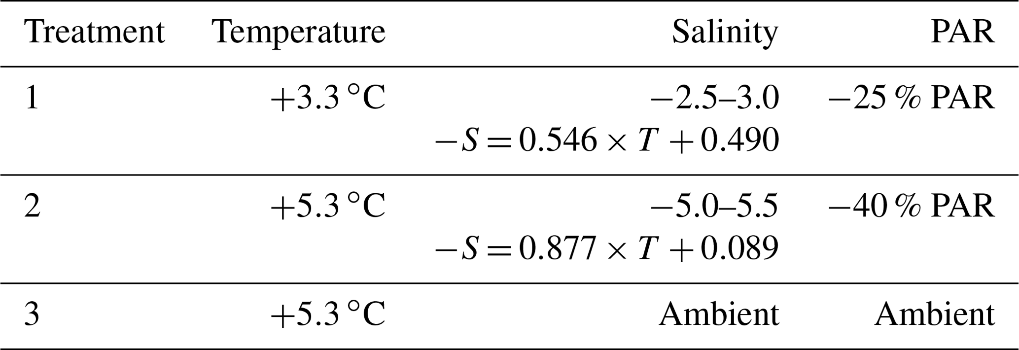
SalTExPreS was utilized to implement three treatment scenarios in a fractional-factorial design to simulate expected future conditions in Kongsfjorden as part of a 54 d experiment that supervised the productivity, survival, and growth response of mixed-kelp communities surveyed at 7 m (maximum depth of collection). The treatments were realized by multi-driver combinations of temperature, freshening, and irradiance, where treatments 1 and 2 differed with respect to the magnitude of temperature increase, salinity decrease, and irradiance decrease (Table 1). Only temperature was manipulated for treatment 3. The chosen treatment and salinity perturbations were applied as offset values from in situ fjord conditions, which were measured at an underwater observatory fixed at 11 m depth and captured the natural variability in the fjord system. The applied temperature offsets used for this experiment reflected the projected Shared Socioeconomic Pathway (SSP) 2-4.5 (SSP2-4.5) and 5-8.5 (SSP5-8.5) scenarios (Meredith et al., 2019; Overland et al., 2019; Table 1). The chosen decreases in salinity were based on correlations between in situ temperature and salinity during summer 2020 in Kongsfjorden (Gattuso et al., 2023), weeks 22 to 35 (Appendix A1 and Fig. A1). These calculated delta salinity values were applied as offsets in treatments 1 and 2 (Table 1). The third treatment scenario applied a temperature change of +5.3 ^∘C as a way to decouple the multi-stressor system and evaluate a temperature-only stress. The effect of turbidity for treatments 1 and 2 was simulated as a decrease in surface irradiance (i.e., ∼ 25 % and ∼ 40 % reduction from ambient irradiance at 7 m, respectively) by applying a combination of neutral light and spectral filters (Lee Filters) placed as static fixtures over the top of the mesocosms. The response of these kelp community assemblages was determined in part by conducting weekly closed-system incubations and assessing the growth and metabolism of the kelp in each mesocosm – details and results of this experiment are discussed elsewhere (Lebrun et al., 2023; Miller et al., 2023a).

Table 1 Experimental treatment conditions with corresponding offsets (compared with the control) for temperature (^∘C), salinity, and photosynthetically active radiation (PAR; expressed as a percentage). See Sect. A1 and Fig. A1 for a full description of the temperature–salinity relationship used to calculate salinity offsets.

2.3 Experimental system

Water was pumped from Kongsfjorden at 10 m depth (300 m offshore) using a submersible pump (Albatros F13T, NPS) that was tapped into an underwater intake pipe and that fed a header tank in the Kings Bay Marine Laboratory in Ny-Ålesund, Svalbard. To prevent clogging from sediment, the pump was situated at 10 m depth, thereby ensuring a safe height above sediment resuspension from the seafloor. Pumped ambient seawater from the header tank was then split into three sub-header tanks within the marine lab with the following conditions: (1) unchanged ambient seawater, (2) ambient water chilled to 0 ^∘C, or (3) ambient water warmed to 15 ^∘C. Each sub-header tank was plumbed to supply a maximum flow of 6 m³ h⁻¹ of ambient, 1 m³ h⁻¹ of chilled, and 2 m³ h⁻¹ of warmed water to each outflow pipe; this required a pressure of 0.3 bar for each line to ensure consistent flow rates (Fig. 1). The three control mesocosms received a mix of chilled and ambient seawater in order to properly simulate in situ temperatures. The three experimental treatments (nine mesocosms in total) received a mix of ambient, warmed, and freshwater for treatments 1 and 2, whereas treatment 3 received a mix of just ambient and warmed water (Fig. 1). Freshwater was sourced from the tap, which is fed by the Tvillingvann reservoir close to Ny-Ålesund. The total flow-through rate of each mesocosm was 0.5 m³ h⁻¹ (i.e., each mesocosm turned over every 2 h) of post-mixed media delivered in an open-cycle flow-through system, which was the necessary flow rate needed to maintain the target nominal values. Continuous flow was maintained throughout the experiment except for weekly 3 h interruptions (to perform experiments on the community) during which the flow to each mesocosm was shut off. In total, there were 12 circular mesocosms (3 treatments and 1 control, each with 3 replicates) with a mean diameter of 1.1 m and a volume of 1 m³, each equipped with a 12 W wave pump (Sunsun JVP-132), a temperature–conductivity probe (PC4E, Aqualabo), an optical oxygen sensor (PODOC, Aqualabo), and an Odyssey light logger. Fiberglass insulation on the outside of each mesocosm reduced unintended changes in the treatment water temperature.

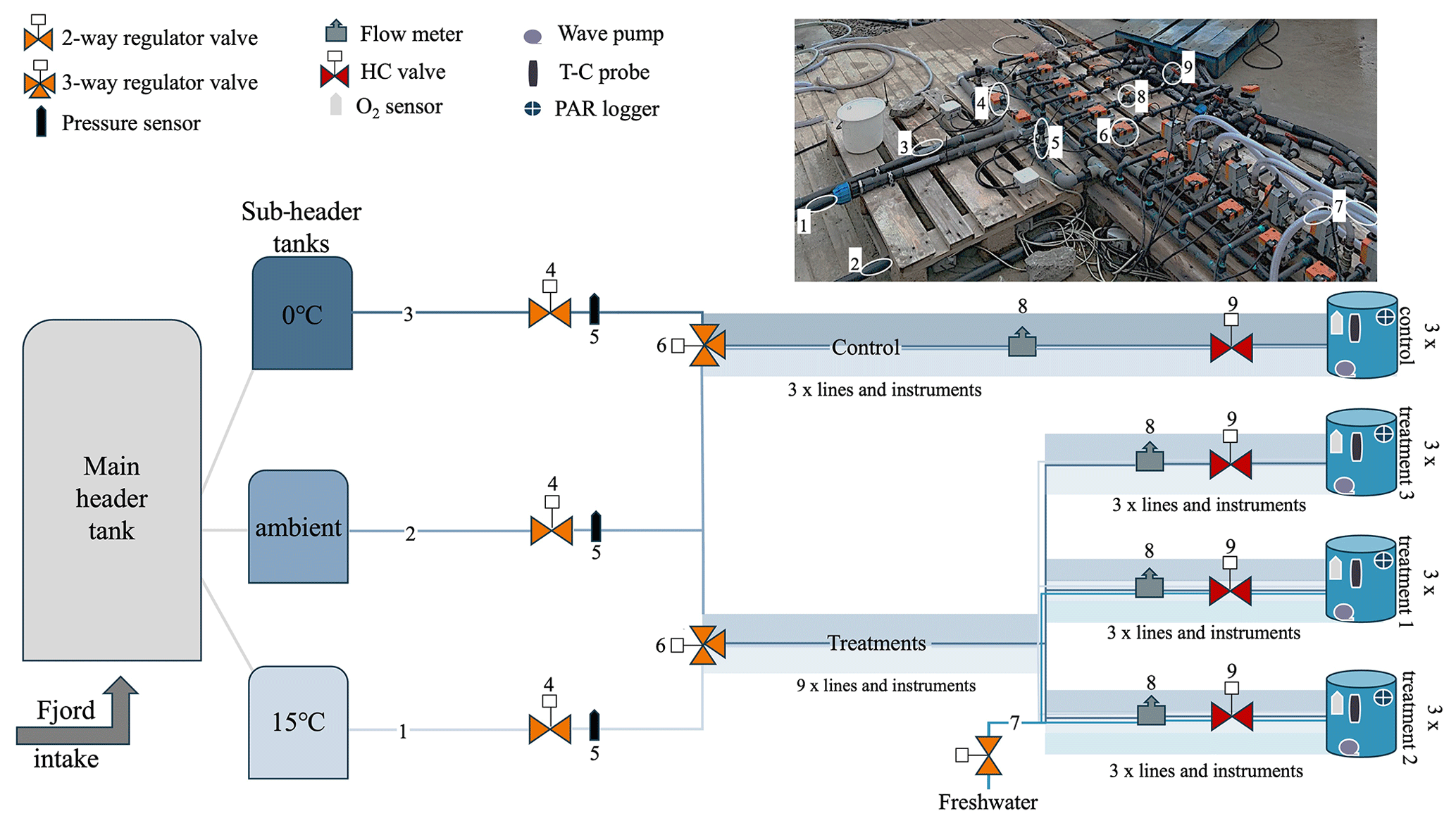
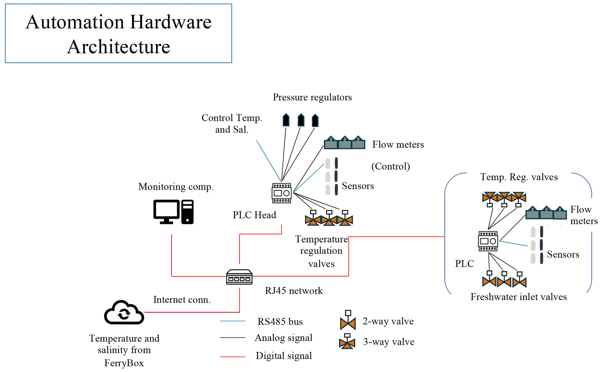
Figure 1 Piping schematic of SalTExPreS, including the mixing and regulation manifold. Items 1–3 depict the main seawater inlets from the warmed, ambient, and chilled sub-header tanks located in the Kings Bay Marine Laboratory. Seawater from each sub-header tank moves through a two-way regulator (4) valve followed by a pressure sensor (5) before splitting into individual lines that lead to all 12 three-way regulator valves (6), each assigned to a single mesocosm. For treatments 1 and 2, the freshwater inlet (clear tube; item 7) passes through a two-way regulator valve before mixing with the ambient- and warmed-seawater lines. Flow rates are then measured (8) post-mixing, and final flow rates are set using a hand-crank (HC) red valve (9). The shaded regions in the schematic indicate that mixed-media lines and instruments occur three or nine times. The T–C probe is the temperature–conductivity probe, and the PAR logger measures the photosynthetically active radiation. Photos of mesocosms and the sensors inside can be found in the Appendix (Fig. A6). Table A1 provides the parts list for the items shown in this figure.

Delivery of ambient, chilled, warmed, and fresh water first ran through an automated mixing manifold that regulated the flow of each media type, ensuring that the proper volumetric proportions passed through the regulator valves to achieve target conditions (Fig. 1). Each source-water flow line was regulated by an automated two-way mixing valve (including the incoming freshwater line) which then passed through a three-way mixing valve that was assigned to each mesocosm (12 in total; Fig. 1). This style of regulation ensured that the proper proportions of manipulated media and ambient water were mixed to achieve nominal conditions. Any temperature variation induced by mixing freshwater was immediately compensated for by regulating the flow of the warm-water line. Details regarding the programmed regulation are discussed further in the Appendix (Sect. A2). The mixed media then passed through a flow meter that measured the flow rate to each mesocosm. A hand-crank regulating valve was placed directly after the flow meter and was used to make minor adjustments and control the overall flow. Measurements by the pressure sensors, the status of the open position for the regulator valves, and flow rates were logged every minute and displayed on the user interface (Fig. A3).

2.4 Nominal regulation

Nominal temperature conditions of +3.3, 5.3, and 5.3 ^∘C, applied to treatments 1, 2, and 3, respectively, were offsets from the nominal control temperature. The nominal temperature of the control was updated hourly and programmed to replicate the measured in situ conditions in the fjord logged by the AWIPEV (Alfred Wegener Institute and Institute Paul Émile Victor) FerryBox part of the COSYNA (Coastal Observation System for Northern and Arctic Seas) underwater observatory (https://dashboard.awi.de/, last access: 28 August 2021) situated at a depth of 11 m. Each treatment condition (temperature and salinity offset) was set by manually programming the nominal value of temperature in the software interface (see Appendix A3). The salinity offset was coupled to the nominal temperature via the correlation described in Appendix A1. The measured temperature and salinity observations from inside each mesocosm were recorded multiple times per minute and used to continuously monitor the regulation of the conditions inside each mesocosm. This data transmission was used to program the software controller that performed the automated regulation of mixed media (see Appendix A2 for details).

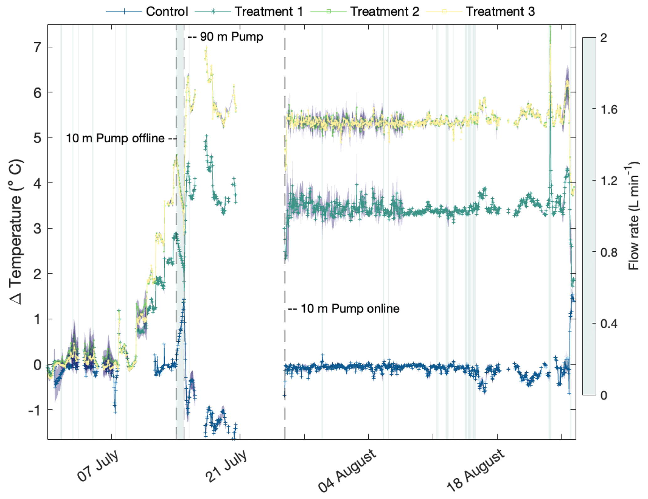
Figure 2 The hourly mean (across triplicate mesocosms) temperature offsets of all applied conditions. For control mesocosms (in blue), offsets were calculated against in situ measurements (FerryBox). For the three experimental treatments (dark green, light green, and yellow for treatments 1, 2, and 3, respectively), offsets were estimated against the mean control values. The purple shaded region around the mean is the standard deviation. The heatmap isoclines (blue-gray shaded regions) are instances in which flow rates were ≤ 2 L min⁻¹ (threshold to avoid large deviations of > 2.0 salinity or temperature). Dashed black lines indicate periods during which the pumps at 10 m depth and 90 m depth were used to feed the sub-header tanks. The time presented is the duration of the experimental deployment.

2.5 Software

The software application used to control SalTExPreS was developed using Visual Studio Community (2019 edition) with the Visual Micro extension and Arduino 1.8.13. The program application has a user-friendly interface designed to allow real-time monitoring and parameterization of regulation processes (Fig. A3). The main window displays each mesocosm condition (the parameters measured by a sensor); their piping connections; a connection status for each programmable logic controller (PLC) that provides information on proper communication, date, and time of the last received communication packet from the head PLC; and the status of the experiment (e.g., started or stopped). The interface also displays the valve-opening percentage along with the nominal pressure and the actual measured value for each main source-water inlet. In addition, the in situ data (temperature and salinity) received from the FerryBox are displayed with the time and date of the last logged value utilized to program the real-time nominal value of the control. Sensor readings of flow rate (L min⁻¹), O₂ saturation (%), salinity, and temperature (^∘C) are shown for each mesocosm in conjunction with the treatment nominal values (i.e., temperature, and salinity when relevant). All measured data are stored through the server connection to the cloud; however, there is a backup microSD card on the head PLC that logs data from all mesocosms every 5 s. If communication fails between the head PLC and the interfaced computer, data will not be retrieved by the PC during the communication break, but they will be retained by the microSD card.

3 Results

3.1 Regulation of the control

The control was able to simulate the ambient fjord temperature well over the experimental period, while the average value across the three replicates deviated < 0.3 ^∘C (Table 2, Fig. 2). The overall quality of the regulation was achieved by the ability of the system to interpret and respond to the measured data from the FerryBox (or to follow a manually programmed nominal value when communication with the FerryBox was interrupted). During the experiment, the FerryBox was intermittently offline 24 % of the time, ceasing the transmission of real-time data and resulting in a break of communication with the PLCs. These somewhat frequent breaks in communication resulted in an average nominal deviation that was nearly 2-fold for the control compared with the treatment conditions (Table 2). The ability to manually program a new nominal value when communication breaks occurred ensured that the control remained robustly regulated. Over the entire period of SalTExPreS deployment, the mean temperature of the control increased from ∼ 4 to 6.5 ^∘C from early July to the end of August (Fig. 3a). The coldest mean temperature of the control occurred when a backup pump situated at 90 m depth in the fjord was used from ∼ 21:00 UTC on 14 July 2021 until 13:49 UTC on 26 July 2021 while the original pump at 10 m depth was repaired. During this period, the control was ∼ 1.0–1.5 ^∘C cooler than the temperature measured by the FerryBox (Figs. 2, 3). As a warmed-seawater inlet was not supplied to the control, the temperature of the control remained cooler than the measured ambient conditions at the FerryBox. Despite the cooler temperature for the control, the regulation of flow rates, mesocosm turnover time, and variability across the control replicates were well maintained by the system.

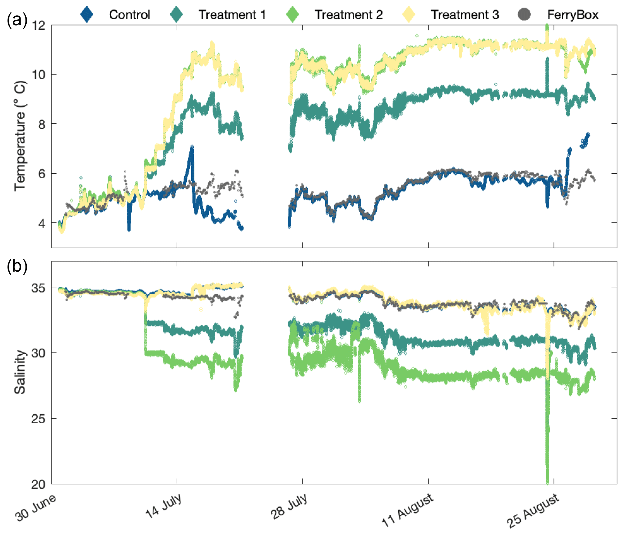
Figure 3 Mean (across triplicate mesocosms) temperature (^∘C; a) and salinity (b) values measured every minute over a 60 d period (including the 6 d period before the start of the experiment) for the control (blue) and for treatments 1–3 (dark green, light green, and yellow, respectively).

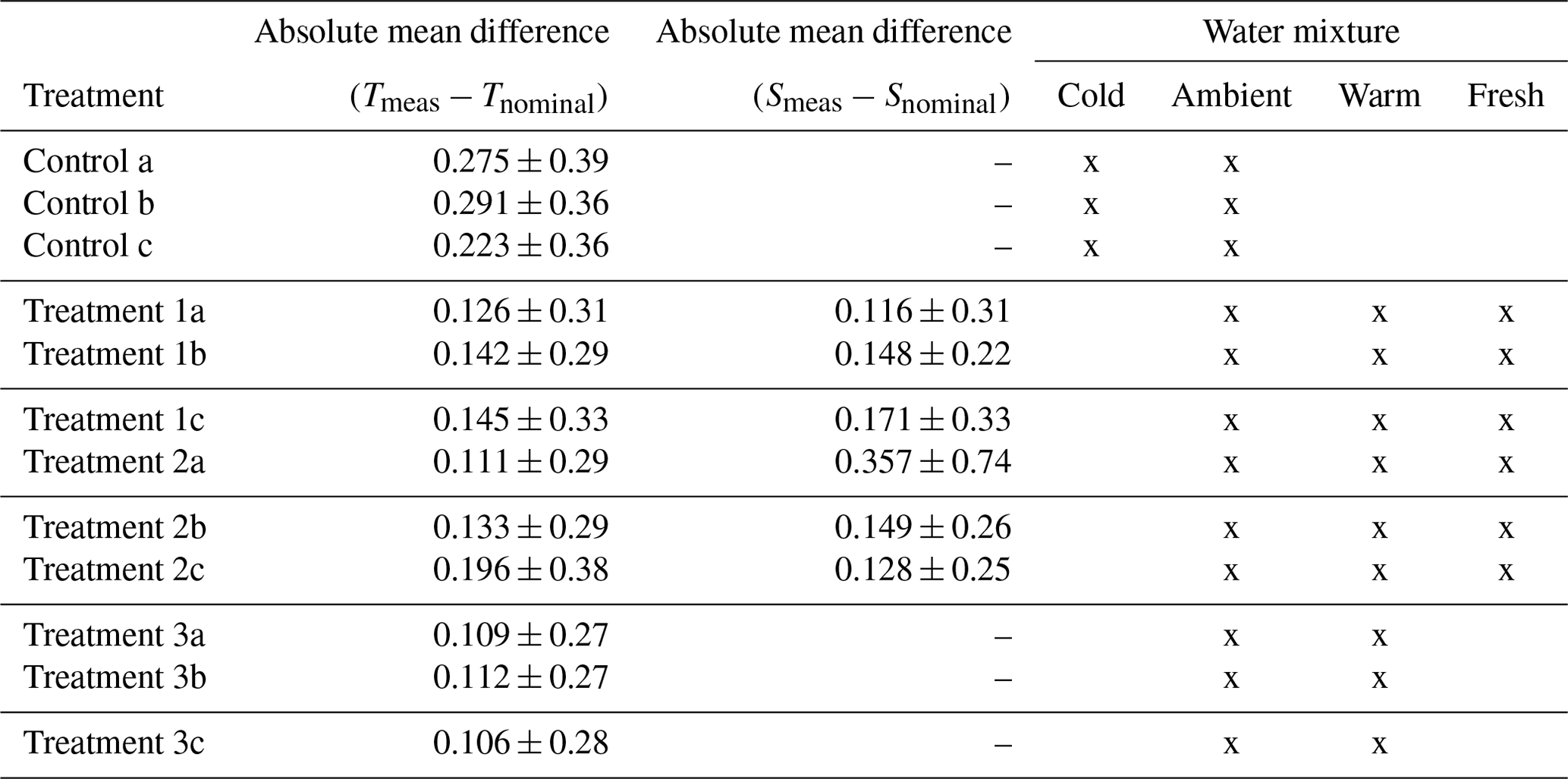
Table 2 Absolute mean difference between measured temperature (T_meas; ^∘C) and salinity (S_meas) values against nominal values (T_nominal and S_nominal), plus or minus the corresponding standard deviation, in each mesocosm during the experimental period. A weighted average was used for treatments 1–3 to account for the initial 5 d incremental increase. Triplicate mesocosms per condition are expressed as a, b, and c. Water mixture indicates the types of media supplied to each treatment, denoted with an “x”.

3.2 Temperature and salinity regulation

The regulation of temperature and salinity under the different treatment conditions (treatments 1–3) was maintained by SalTExPreS for the full planned duration of 54 d 3 July to 26 August 2021 (full data set available: Miller et al., 2023b). For the first 6 d of the SalTExPreS experiment, the treatment conditions were held at the control (i.e., no applied offset from the control) before the stepwise increase in temperature began. At 12:00 UTC on 10 July 2021, a temperature offset of 0.55 ^∘C d⁻¹ was programmed for treatment 1, whereas treatment 2 and 3 were programmed to increase by 0.88 ^∘C d⁻¹ (Figs. 2, 3). The final nominal temperature above the control was reached at 21:00 UTC on 15 July 2021. The system needed 4 h to achieve the new temperature conditions (i.e., homogenize the mesocosm to a 0.88 ^∘C increase). A manual override was applied to the salinity regulation for treatments 1 and 2, resulting in the system achieving the final salinity offset value upon the initial temperature increase (Figs. 3b, 4). This was done to ensure the maintenance of salinity regulation as the temperature offsets were applied relative to the control, which was receiving fjord water pumped from 90 m and was colder than the measured in situ conditions. It took the system 4 h to achieve the salinity offset for treatment 2, adjusting the value from ∼ 34 to 29.8 (Figs. 3b, 4).

The precision of the temperature and salinity regulation across all treatment conditions was well maintained, as the mean difference between the measured value and the nominal value was < 0.2 ^∘C and < 0.36 for salinity across the entire deployment (Table 2). The mean deviations observed across treatments did not appear to correlate with the degree of offset. Thus, treatment 3 showed the highest precision for temperature regulation, whereas salinity regulation was the most robust for treatment 2 compared with treatment 1 (Table 2). During several instances in which communication was interrupted between the FerryBox and the head PLC, SalTExPreS retained the last measured value at the FerryBox as a contingency protocol. This aided the system to maintain a high degree of regulation throughout the entire deployment. The largest deviation from the nominal value for all treatment conditions occurred during a single instance in which the last read value from the FerryBox was not retained: this occurred at 04:47 UTC on 24 August 2021 (Fig. 4). Communication was quickly restored after this incident by cycling the program code, and the average deviation of temperature (^∘C) and salinity for treatment 1 for the remainder of the deployment was < 0.16, whereas this value was < 0.25 for treatment 2.

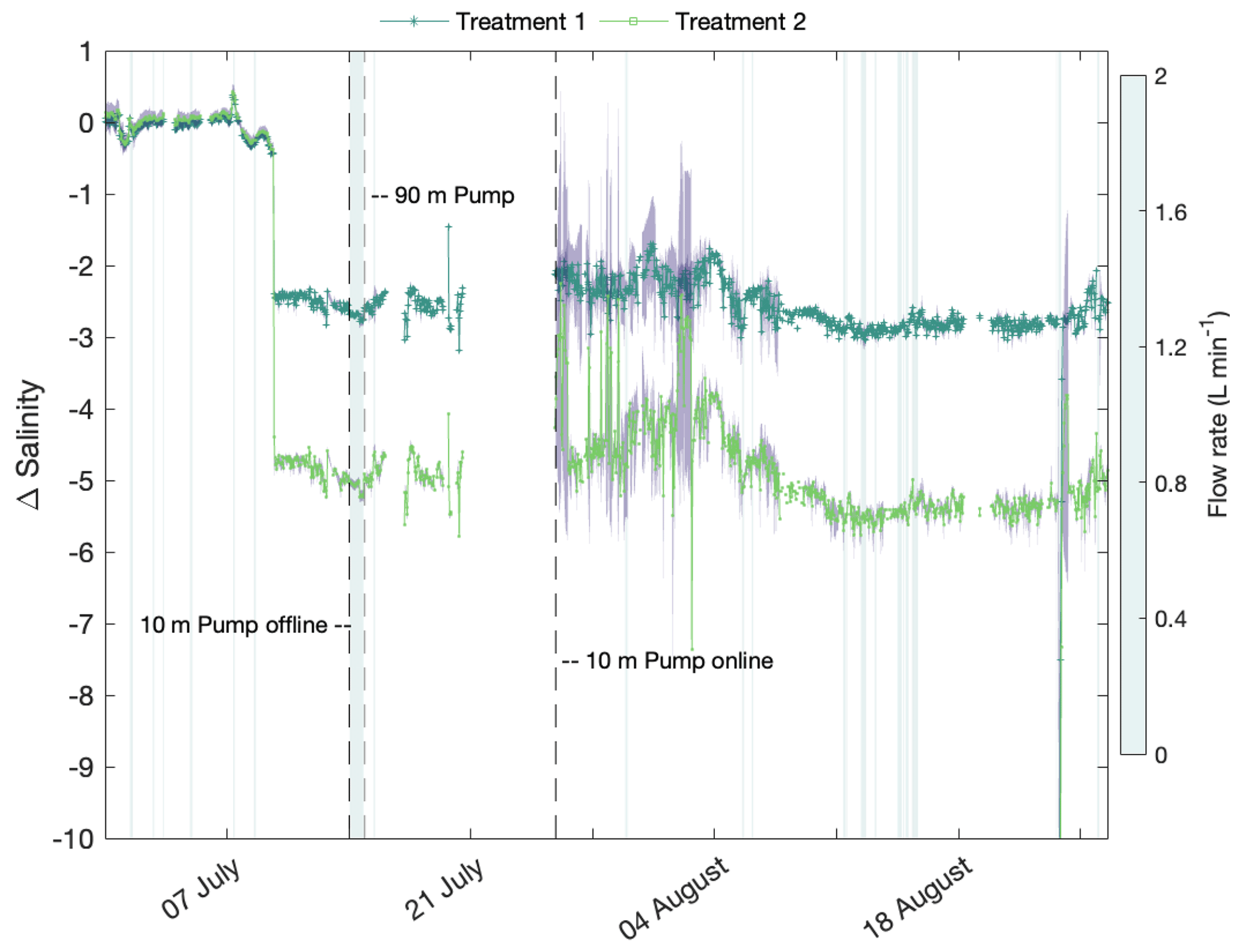
Figure 4 The hourly mean (across triplicate mesocosms) salinity offsets for the experimental period. Dark green is treatment 1 and light green is treatment 2. The purple shaded region around the mean is the standard deviation and the heatmap isoclines (blue shaded regions) are the instances in which flow rates ≤ 2 L min⁻¹. Dashed black lines indicate periods during which the pumps at 10 m depth and 90 m depth were used to feed the sub-header tanks.

When adequate flow rates were maintained, SalTExPreS was able to simultaneously regulate 12 mesocosms under 4 different conditions to deviations in temperature and salinity that were < 0.5 ^∘C or 0.5 from the nominal value ≥ 80 % and ≥ 70 % of the time, respectively (Fig. 5). Due to an erroneous nominal value for the control during the 90 m pump usage, these times were excluded. If warm water could have been mixed with the ambient water feeding the control mesocosms, a proper nominal value could have been maintained. Over the full duration of the experiment, effective regulation from the nominal temperature and salinity values were kept to < 1 for all mesocosms 89 % of the time for temperature (^∘C) and 80 % for the salinity (excluding the first replicate for treatment 2).

4 Discussion

The first application of the fully autonomous SalTExPreS demonstrated the capacity of the system to successfully manipulate temperature and salinity as an offset value from the control, thereby maintaining natural, in situ variability for four different conditions simultaneously. We utilized this deployment to test the effects of climate change drivers on Arctic kelp communities, recognizing the feasibility of the system to perform ex situ experiments on organisms or whole communities (Miller et al., 2023a). The versatility of the system not only allows for the manipulation of temperature and salinity but also for the incorporation of other factors such as CO₂ or hypoxia. While this experiment used a control offset approach to produce treatment conditions, programmable parameterization of various treatment combinations can be applied depending on the question and design of the experiment. The automated component of the system reduced the logistical hurdles that can arise when performing high-precision replication and regulation of experimental conditions that track real-time system variability. While the use of such a system can reduce user oversight and limitations, there is still a need for diligent operation.

Since the initial experiment, we have implemented a number of changes to improve the performance of the system; these improvements have been realized during a second experiment in the summer of 2022 (Fig. 6). In the 2022 experiment, SalTExPreS was integrated to function with a deployable heat pump to simulate multiple scenarios of marine heat wave patterns over a nearly monthlong experiment. In this instance, temperature regulation was vastly improved as a result of the programmable modifications made since the initial experiment. During this second experiment, SalTExPreS mimicked three marine heat wave scenarios where dynamic temperature regulation kept deviations in the nine different mesocosms at < 0.5 ^∘C for 94 % of the time. This was a ∼ 15 % improvement of temperature regulation time compared with the first experiment. During the first experiment, inconsistent flow rates and communication errors between the FerryBox and the head PLC were the primary causes of larger deviations (> 2.0 for salinity or temperature) from nominal values. For example, flow rates of < 2 L min⁻¹ accounted for ∼ 20 % of the large deviations in temperature and salinity regulation. Simple software modifications, such as pop-up alert windows that warned when a lapse in communication with the FerryBox occurred (e.g., FerryBox stopped logging) as well as the addition of contingency coding instructions (i.e., fail-safe instructions) ensuring that the last received in situ data were maintained, solved most of the issues. Communication errors were easily remedied by cycling the power on a PLC, which is why pop-up alerts were an improvement to the operation. Other extraneous circumstances that could impact flow rates, such as pump failure and clogging of the seawater intake ports, are issues that need to be addressed whenever SalTExPreS is used; however, these are very manageable situations that can be easily mitigated by an operator.

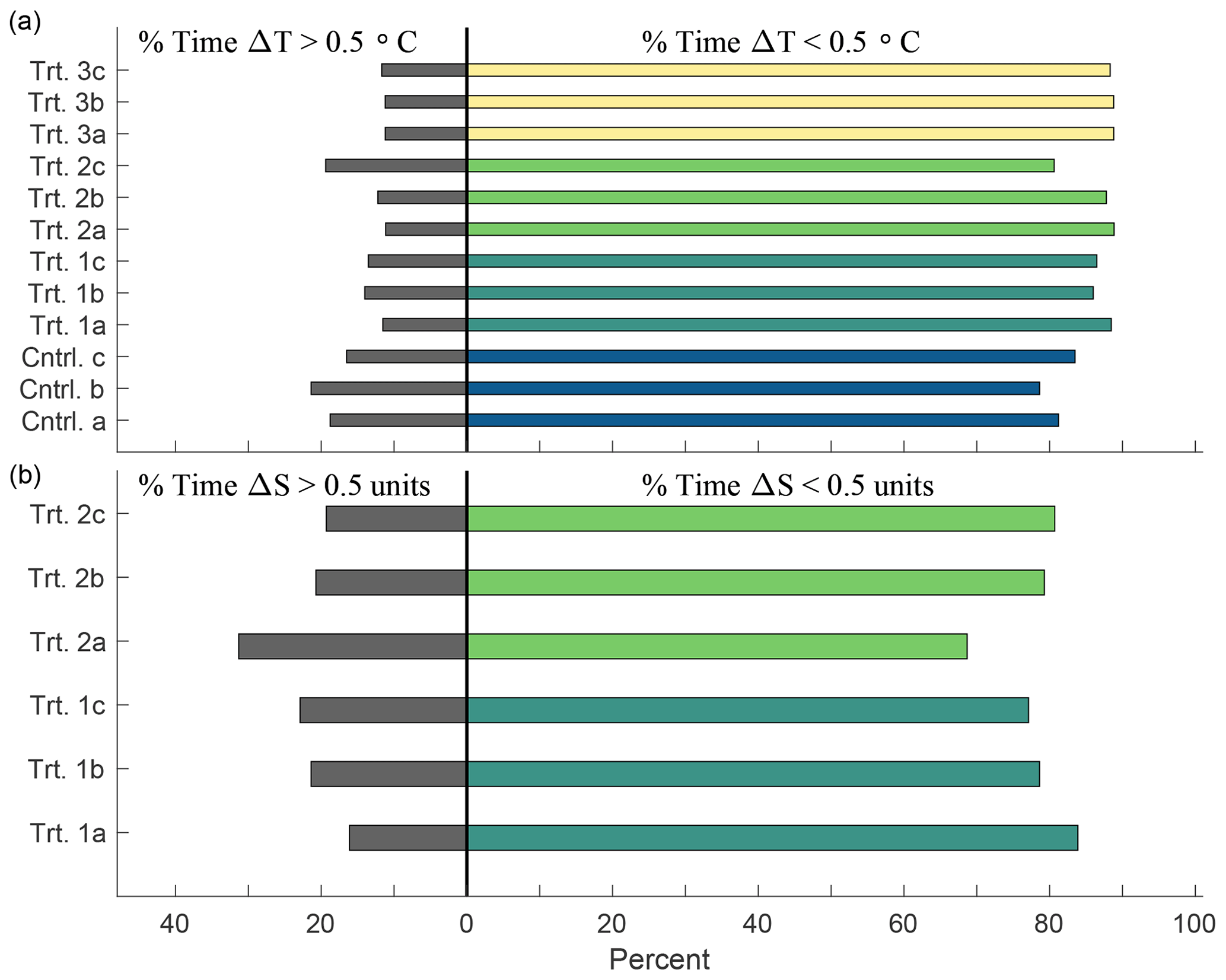
Figure 5 The percentage of time that each mesocosm experienced a deviation greater than (black bars) or less than (colored bars) 0.5 ^∘C (ΔT; a) or 0.5 in salinity (ΔS; b) when flow rates were above 2 L min⁻¹. “Cntrl.” or “Trt.” are used to refer to the control or treatments, respectively. This excludes the period during which the 90 m pump (12 d) was used but accounts for 42 d out of the 54 d of the experiment. The bar color indicates different treatment groups, as shown on the y axes.

The novelty of SalTExPreS lies in its ability to independently regulate experimental conditions in a single experimental chamber (e.g., mesocosm). The operational data produced from this deployment are reliable, easily quantifiable, and provide the highest degree of monitoring frequency for every applied experimental condition. This study has demonstrated the system's ability to replicate dynamic nearshore environments, in which temperature and salinity can vary at a high frequency (e.g., tidally). The system's additional capacity to mimic future scenarios by applying an amplitude offset to the natural dynamics of in situ conditions is an added feature for conducting manipulative experiments. Wahl et al. (2015) described a system with a similar capability, but they regulated treatment conditions by monitoring the source water and adjusting that media before it was delivered to each experimental chamber. SalTExPreS differs in that it measures the conditions inside each experimental chamber (i.e., mesocosm) and regulates them independently based on per second measurements. This provides the flexibility to individually modulate each experimental chamber, thereby offering a broad range of versatility. The lack of infrastructure needed to set up SalTExPreS makes it easy to deploy and transport. As long as there is a sufficient supply of ambient water and manipulated media, there is little limit to the versatility of automated control for each mesocosm. Many research endeavors and future implementations of SalTExPreS have the potential to model a large range of experimental settings that pertain to the environmental perturbations associated with climate change or other anthropogenic forcings. The operation of such a system under extreme environmental conditions has shown the durability of the manifold to endure an adverse Arctic summer and still respond without mechanical failure. With proper operation and user proficiency, this proves to be a highly sophisticated and powerful tool to be utilized for marine and aquatic perturbation experiments.

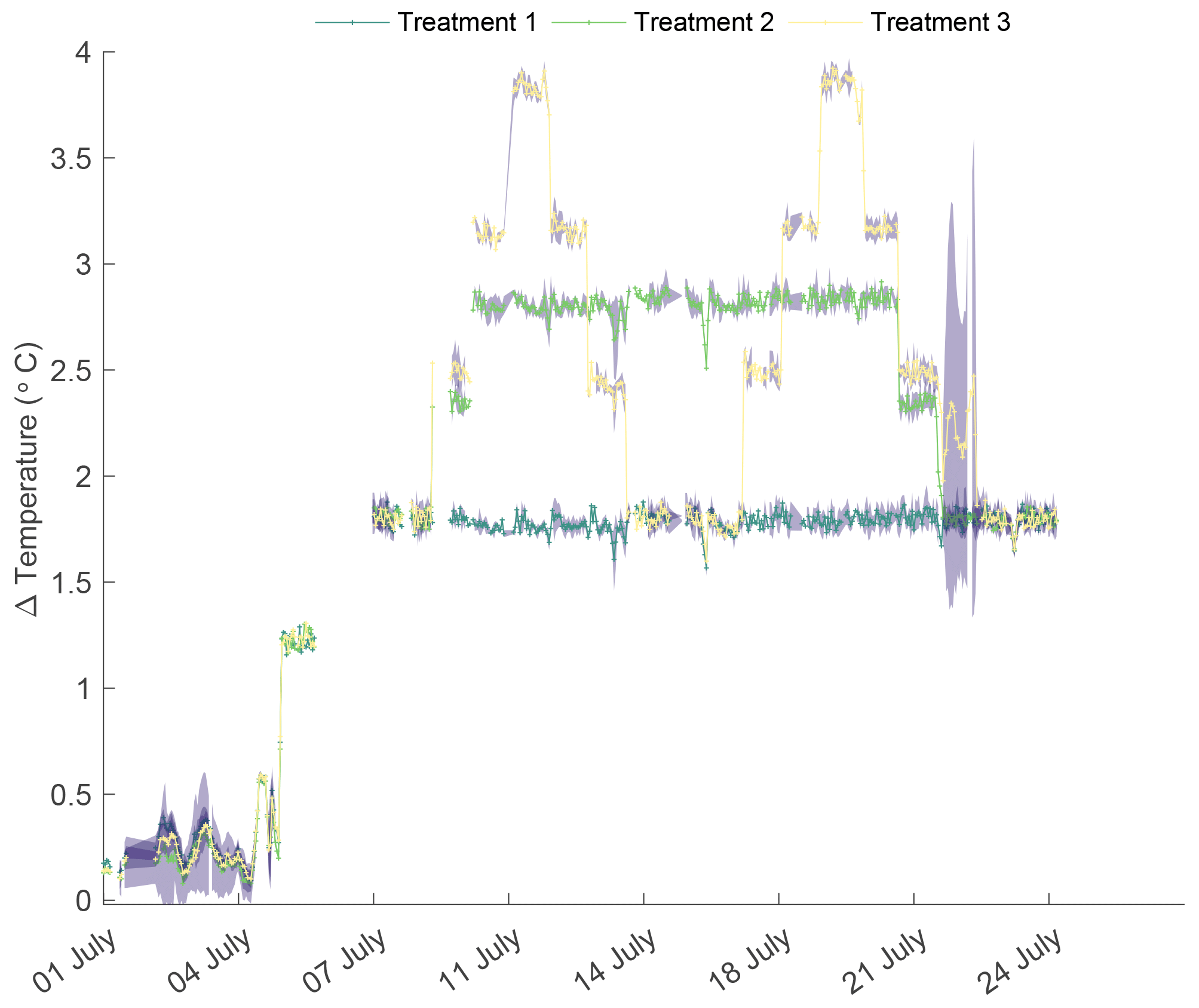
Figure 6 The hourly mean temperature offsets (Δ Temperature) during the second deployment of SalTExPreS in the summer of 2022 in Tromsø (Norway) during which a variation of heat wave scenarios were performed with experimental treatments 1–3. Treatment 1 is a constant high temperature (+1.76 ^∘C), treatment 2 is a low-frequency (one heat wave) and medium-magnitude offset (+2.81 ^∘C), and treatment 3 is a high-frequency (two heat waves) and high-magnitude offset (+3.86 ^∘C). The purple shaded region around the mean is the standard deviation.

Appendix A

A1 Calculation of salinity offset

In the summer of 2020 (weeks 22 to 35), the mean temperature at 11 m displayed a range of 2.48–6.28 ^∘C, with salinity values ranging from 34.67 measured at the minimum 2.48 ^∘C to 33.63 measured at 6.28 ^∘C (Fig. A1a). The correlation was best fit with a second-order polynomial. To project the salinity offset at a future temperature based on this second-order polynomial fit, temperatures of +3.3 and 5.3 ^∘C (SSP2-4.5 and SSP5-8.5, respectively) were added to in situ fjord temperatures and salinity was calculated based on the second-order polynomial. These estimated salinity values were then subtracted from the mean salinity values observed (y axis in Fig. A1a) in summer 2020 in order to calculate a delta salinity value for the SSP2-4.5 and SSP5-8.5 scenarios. The relationship between these estimated delta salinity values and the mean in situ temperature (x axis in Fig. A1a) displayed a robust linear relationship (Fig. A1b).

Table A1 Parts list with manufacturer model numbers.

A2 Temperature and salinity regulation

Accurate temperature and salinity regulation was managed using the software PID (proportional integral derivative) controller on the corresponding PLC. The PLC operated in PoE (power over ethernet) mode, which builds a local area network (LAN) and enables the use of ethernet data cables to carry electrical power. The PID controller measures the difference between the measured value and the nominal value (i.e., the error). This calculates the position and adjustment of the valve opening by multiplying the error, the integral of this error, and the derivative of the error over time by the previously determined coefficients K_p (proportional gain), K_i (integral gain), and K_d (derivative gain), respectively. These coefficients were obtained experimentally using the empirical method of Ziegler and Nichols (1943). These coefficient values may differ from one condition to another.

Table A2 Functions used for the programming of software.

A2.1 Pressure and flow regulation

Each sub-header tank inlet line of ambient, chilled, and warmed seawater had its own pressure regulation system, enabling equivalent pressure levels to be maintained. This regulation process aided the system's ability to adjust flow rates for all mesocosms using the hand-crank valves (Fig. 1). The system consisted of an analog pressure sensor (Siemens 7MF1567-3BE00-1AA1) and a two-way analog valve (BELIMO R2025-10-S2 with an LR24A-SR motor). The pressure sensors were placed inline directly after water from each sub-header tank passed through a regulator valve. The sensor ensured that the pressure for each line was maintained at 0.3 bar by transmitting data to the system which then regulated the valve-opening position of the incoming flow. A nominal pressure for all three sensors was predetermined during flow rate test trials. This process took place during the setup of the system and involved the valve opening being adjusted using a PID regulator (see Sect. A2) to maintain the defined nominal pressure.

A2.2 Automation

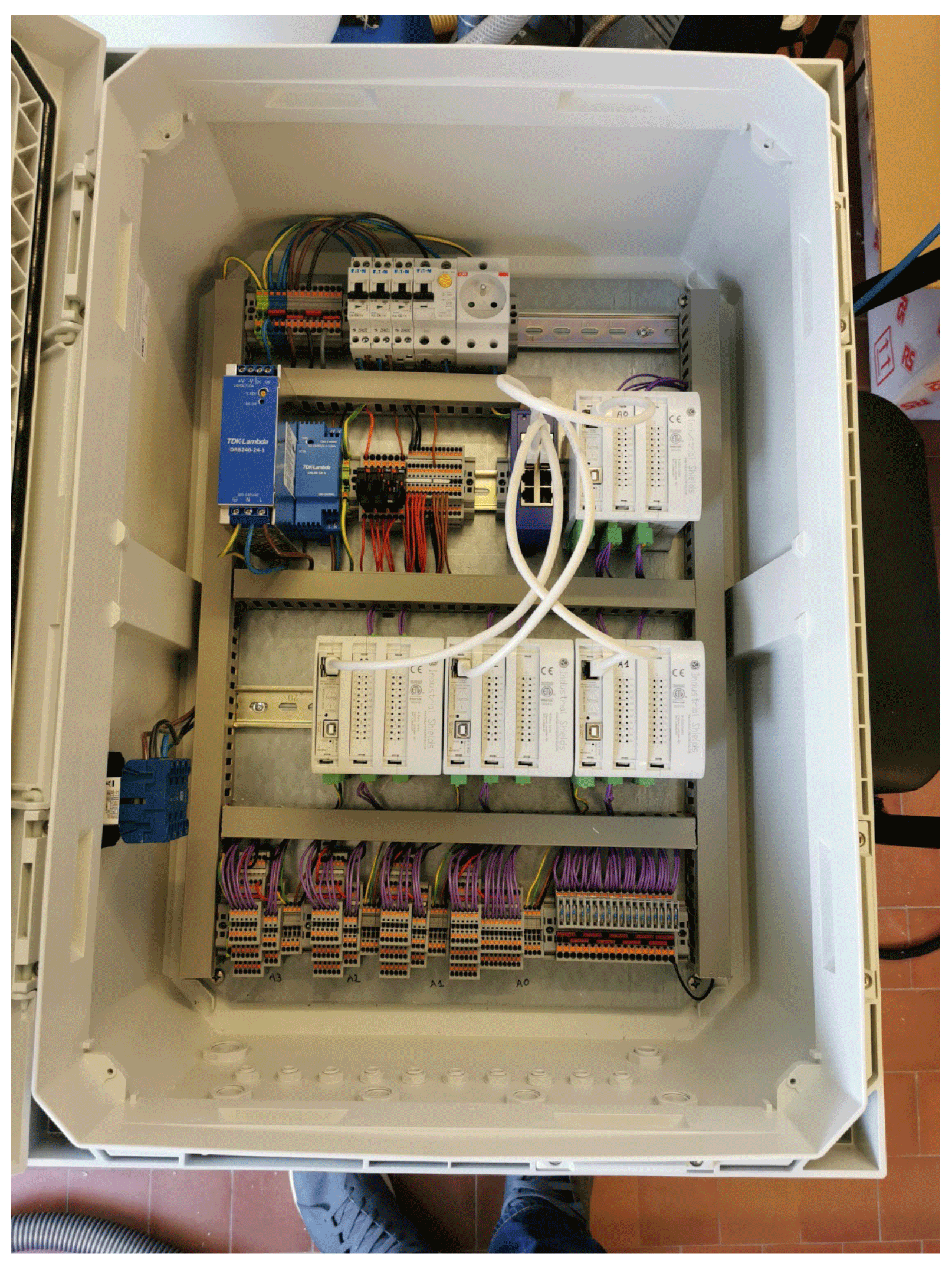
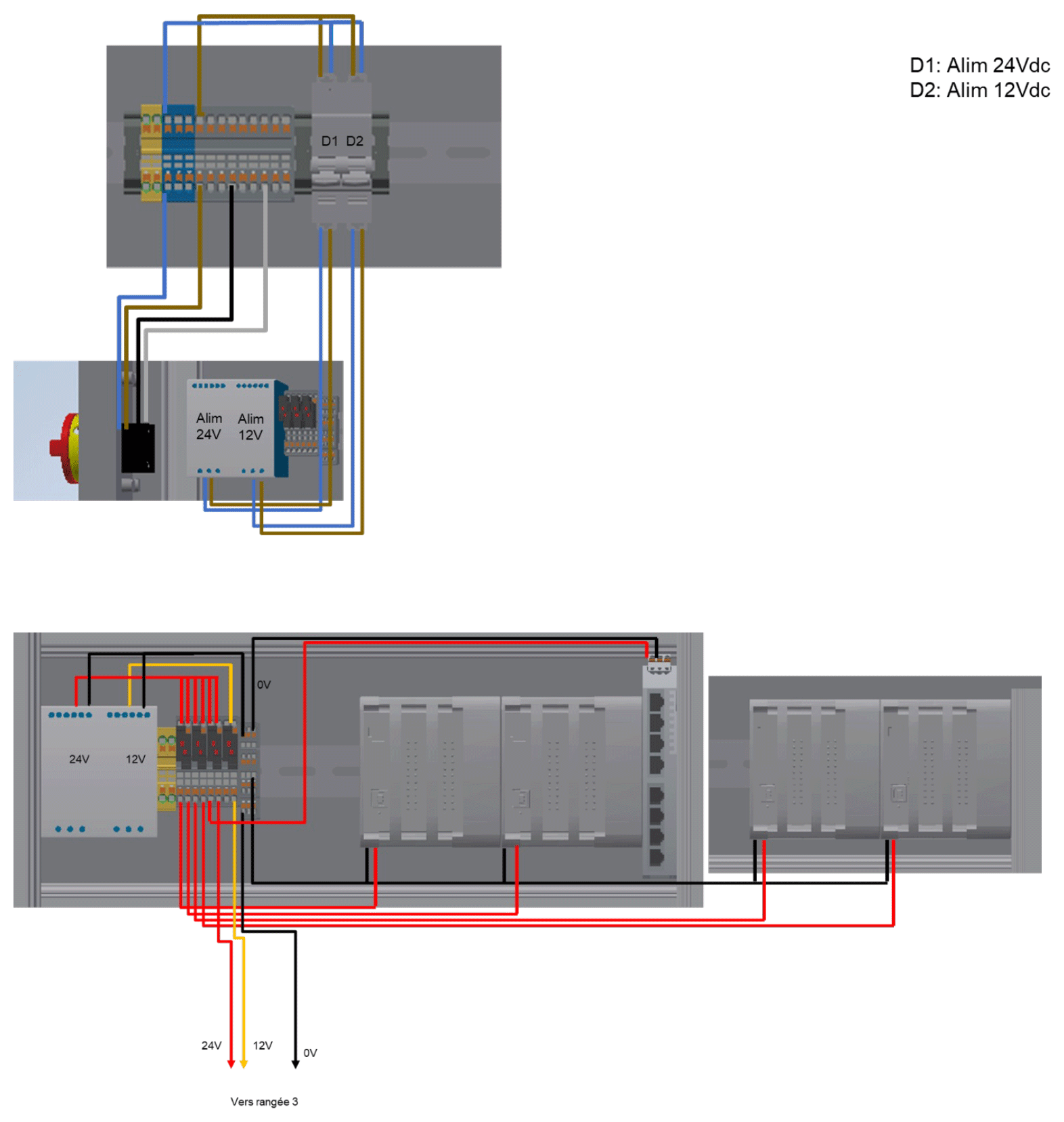
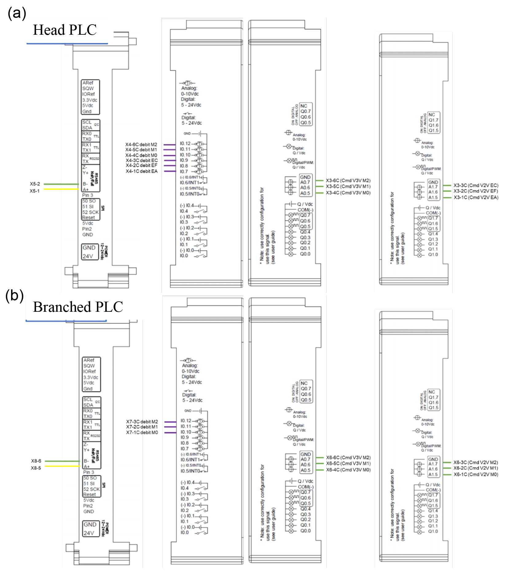
The automation was performed using four Industrial Arduino-based PLCs (MDuino.42+, Industrial Shields), with an individual PLC regulating the control and each treatment (1–3), respectively. Each PLC was responsible for logging data and regulating a specific experimental condition. The PLC regulating the control – identified as the head PLC – was the primary device responsible for communication with the branched PLCs and the monitoring computer (Fig. A2). All monitoring was performed on a PC Windows application (Sect. A3) that was responsible for the following: (1) reading data received from the PLCs, (2) reading in situ data received from the internet, (3) displaying live data, (4) logging data and sending it to a file transfer protocol (FTP) server, and (5) sending settings and commands to the PLCs. Communication between the PLCs and the PC was ensured using HTTP WebSocket protocol on RJ45 ethernet cables. The communication between the PLCs and the conductivity–temperature and oxygen sensors, flow rate sensors, and regulation valves was executed using a half-duplex RS485 (two wires) protocol, with an analog 4–20 mA and an analog 0–10 V signal, respectively. All PLCs and wired communication lines were housed in an electrical box installed in an IP68 Fibox enclosure with a 400 V ($\mathrm{3}P+N+E$; three-phase, neutral, and earth/ground), 32 A security switch (Fig. A6). All of the automation elements use low tension (12 or 24 V DC) through circuit breakers and fuses. The electrical box was protected with a 220 V socket.

A3 Software development

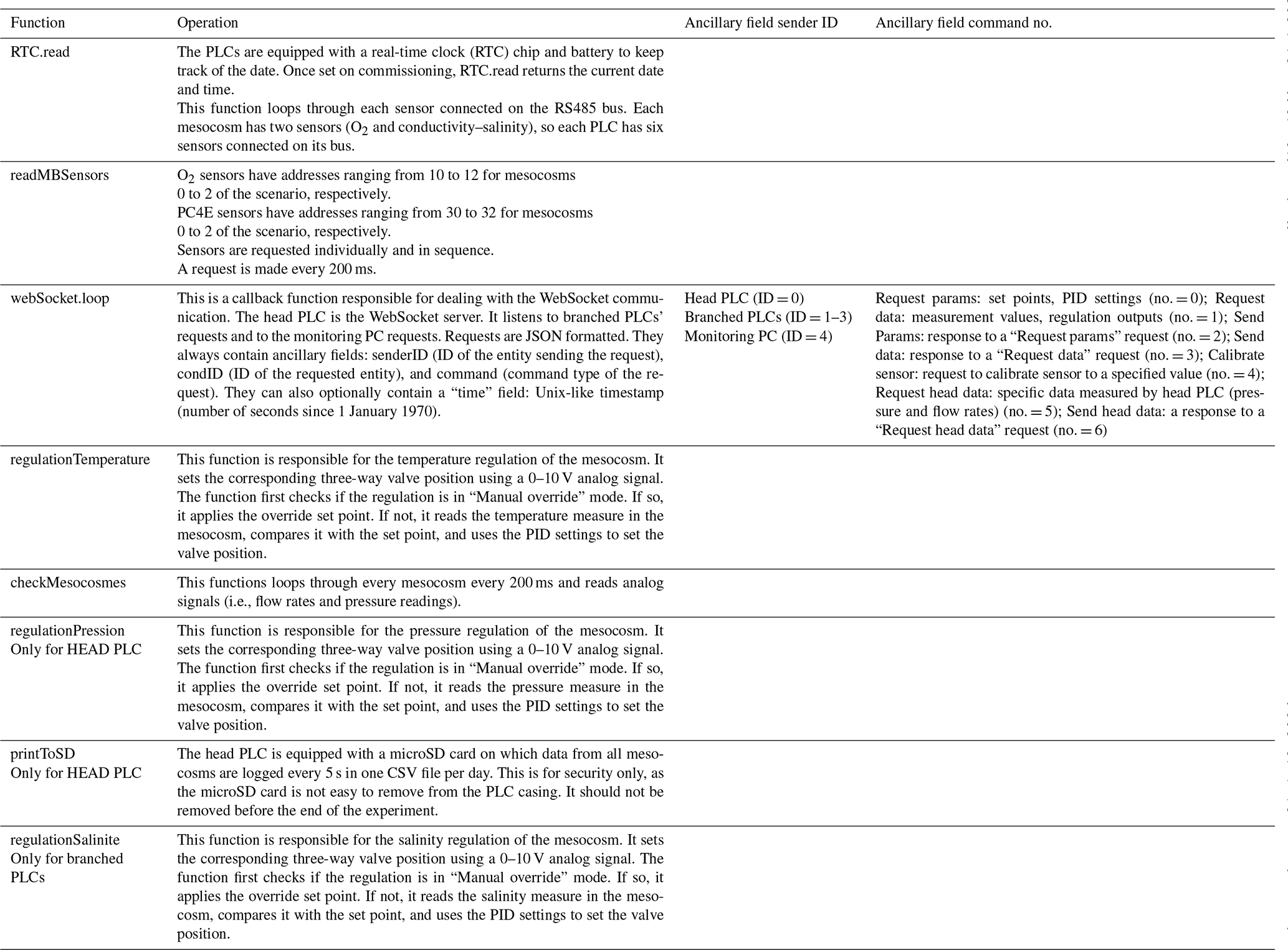
The code for the application was written in C and C$++$. The code uses publicly available Arduino libraries (https://www.arduino.cc/reference/en/libraries/, last access: 14 March 2021) as well as originally designed libraries. All code is available on GitHub (https://github.com/purrutti/FACEIT, last access: 30 June 2021). The code is divided into two pathways: “Master.ino” for the head PLC and “Regul_condition.ino” for the branched PLCs. A description of the main functions applied in the code for programming the system regulation and features are listed in Table A3.

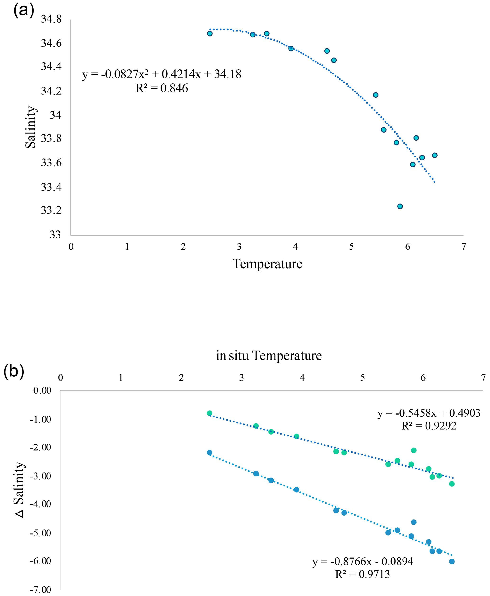
Figure A1 (a) Relationship between temperature and salinity in summer 2020 (weeks 22–35) in Ny-Ålesund, Svalbard. (b) Relationship between estimated delta salinity and in situ temperature, where delta salinity was calculated as the difference between the current mean salinity and the salinity estimated at the temperature increase projected for the SSP2-4.5 (green dots) and SSP5-8.5 (blue dots) scenarios.

A4 Menu bar of the PC application

From the interface, the user sets the temperature condition and associated salinity offset, IP address and logging parameters, sensor calibration settings, and nominal pressure (Fig. A4).

Within the menu bar, several tabs permit the setup of the project: File, Settings, Maintenance, and Data. Under “File”, the system can be manually connected to, or disconnected from, the PLCs. Connection is usually maintained automatically. The “Settings” tab displays the application and experimental setting options (Fig. A4a–c). All of the settings of the project are stored on the computer (found in “Application settings”) that is running the application, including the following:

• i.

  head IP address – the IP address of the head PLC (centralizing all the data);

• ii.

  data query interval – frequency of queries from the application to the head PLC;

• iii.

  data log interval – number of minutes between logs to file;

• iv.

  database file path – directory and base filename of the CSV data files;

• v.

  FTP username, password, and path – FTP settings for sending the data file every hour;

• vi.

  InfluxDB settings – for live monitoring and local storage of the data.

Under “Experimental settings”, the programmed specificities and regulation of the treatment conditions can be adjusted. This includes programming the nominal pressure (all main inflow lines), the temperature, and the salinity–temperature relational equation (on a different tab selected from a drop-down menu) as well as adjusting the K_p, K_i, and K_d coefficients for the regulation. The nominal temperature is provided by the data received from the FerryBox; however, this can be overridden if needed. The “Save to PLC” button sends the values to the corresponding PLC and saves the data, while the “Load from PLC” button loads the settings from the PLC. For the purposes of this experiment, the nominal salinity was calculated based on a delta salinity for treatments 1 and 2 that was derived from the linear relationship with temperature. This can also be overridden, if needed, by selecting the manual override box.

Figure A2 Diagram and flowchart of the automation system.

The “Maintenance” tab is where sensor calibration and communication “Debug” operations can be executed (Fig. A4d, e). Calibration can be performed for each sensor deployed in each mesocosm, and it uses a two-point calibration for temperature and oxygen percentage. The salinity calibration is done by setting the conductivity value corresponding to a temperature of 25 ^∘C, rather than the in situ measured temperature. The conductivity value is programmed as µS cm⁻¹. The communication process for sensor calibration is between 5 and 10 s. The final option in the menu is the “Data” tab which displays the historical and live data. The historical data can be interfaced to a HTML site if desired.

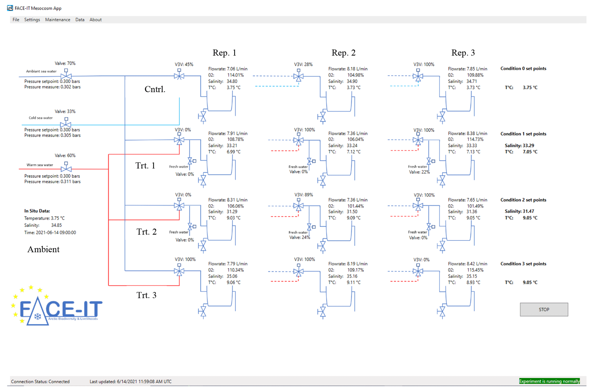
Figure A3 Application interface displaying real-time monitoring of ambient conditions as well as the control (Cntrl.) and treatment (Trt.) conditions for each replicate (Rep.) in each mesocosm.

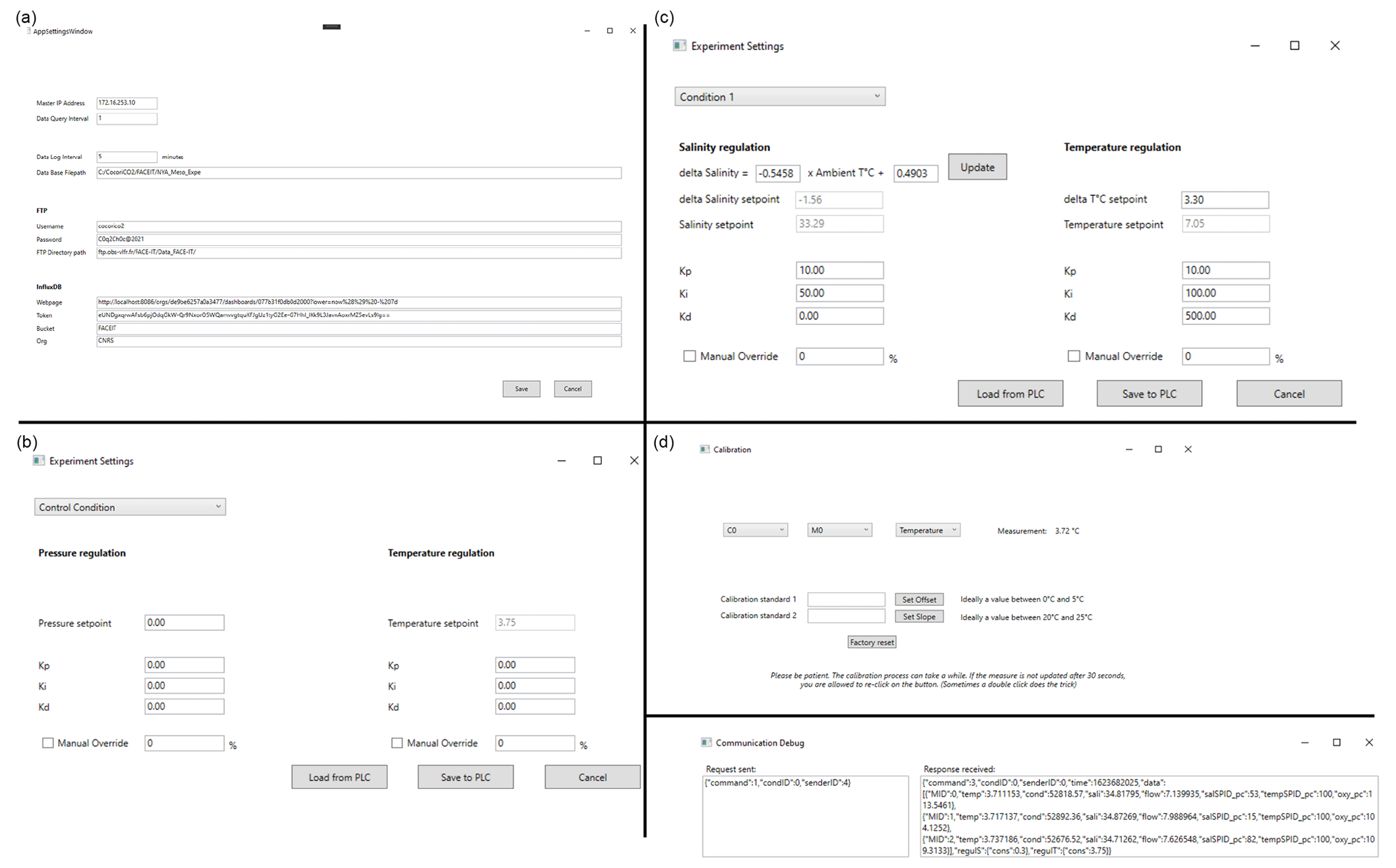
Figure A4 Operation windows for the application and experimental settings (a–c), found under the “Settings” tab, and operation windows for sensor calibration and debugging (d, e), found under the “Maintenance” tab.

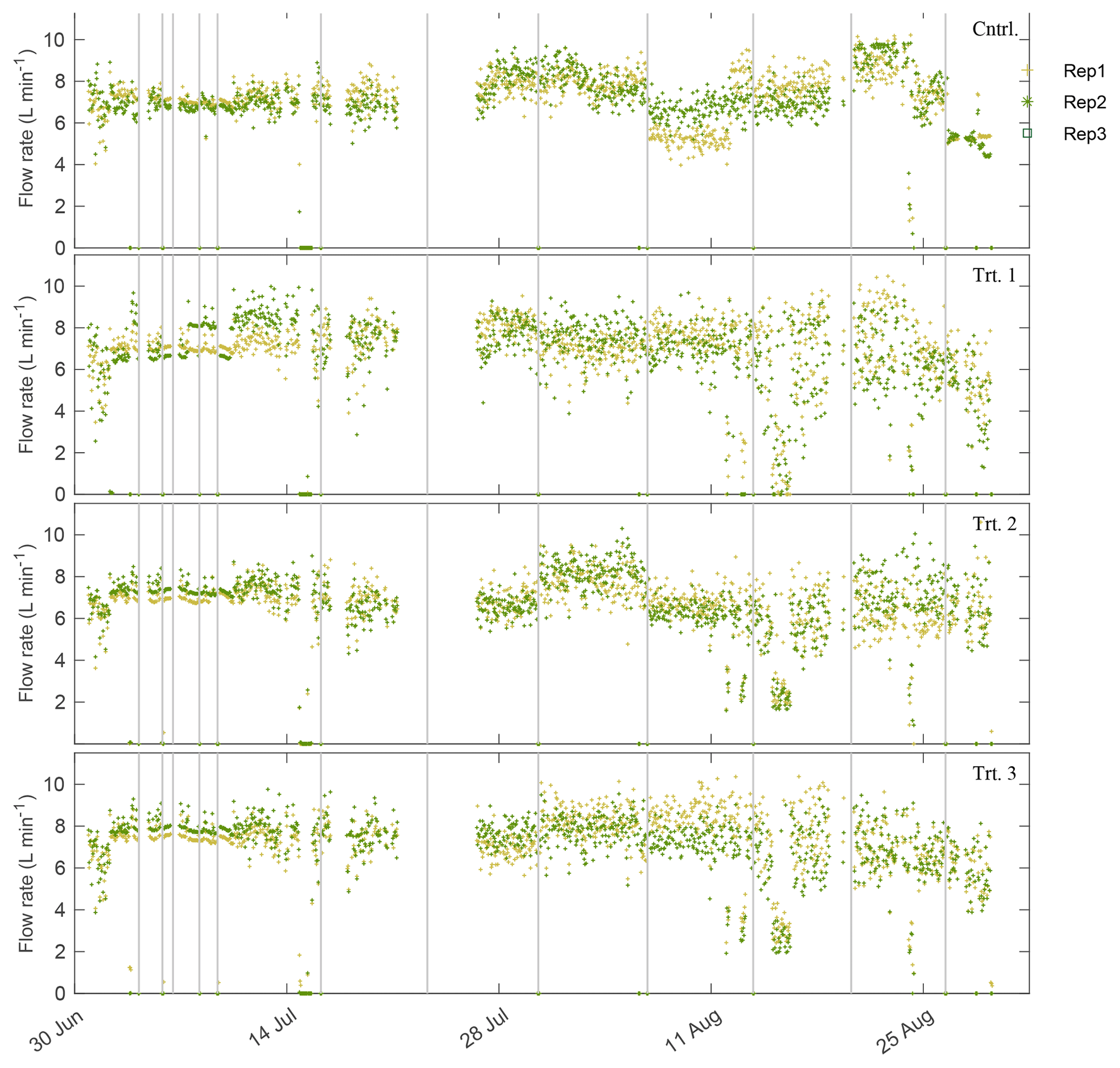
Figure A5 Flow rates for the control (Cntrl.) and treatment (Trt.; treatments 1–3) conditions for the entirety of the system deployment. Black vertical lines are when incubations were performed and the system shut off for a period of 3 h; flow rates went to zero at these times.

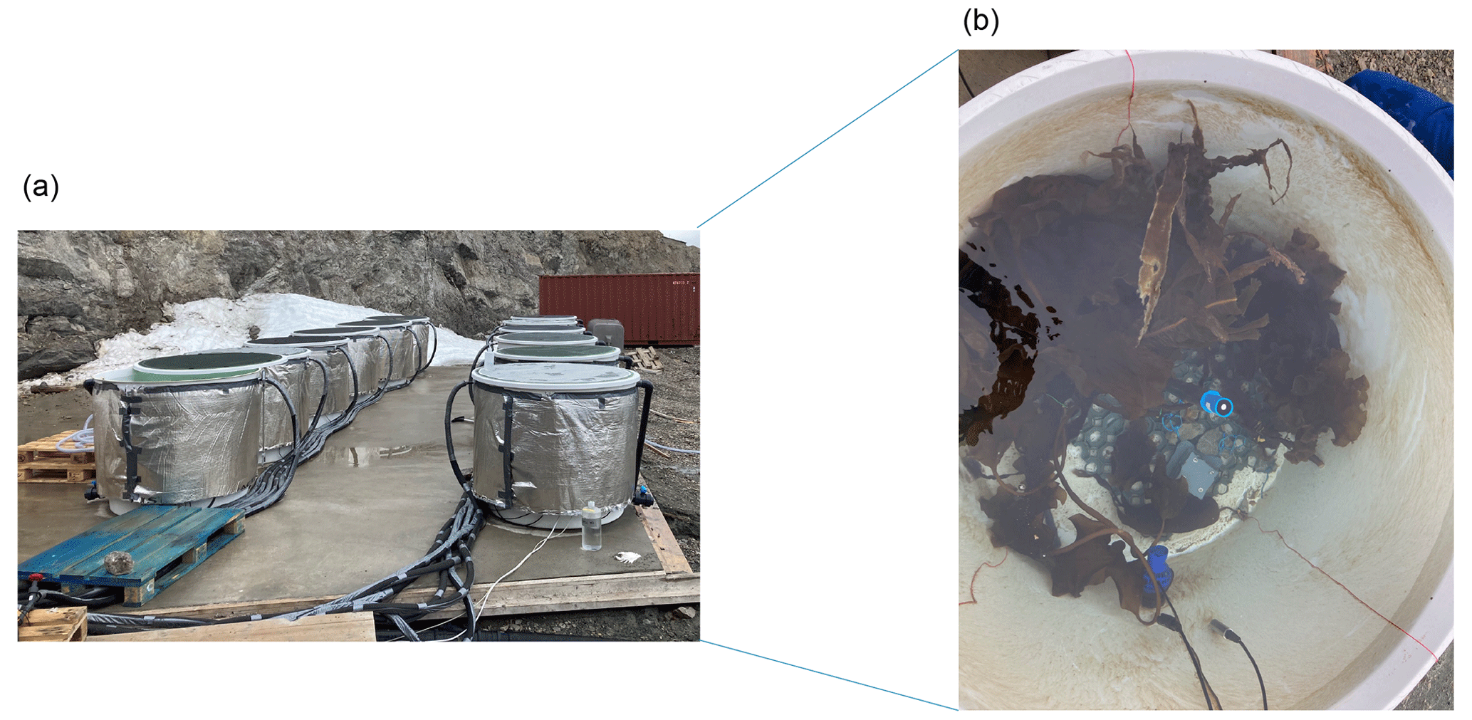
Figure A6 All 12 mesocosms are displayed in panel (a). The inside of one mesocosm is detailed in panel (b), showing the oxygen and temperature–conductivity sensors along with the photosynthetically active radiation (PAR) logger in the bottom right of the photograph.

Figure A7 The electrical cabinet used for SalTExPreS.

Figure A8 The electrical schematic for wiring within the electrical box.

Figure A9 The PLC controller diagram for the head (a) and branched (b) operations.