The influence of plant water stress on vegetation–atmosphere exchanges: implications for ozone modelling

Evapotranspiration is important for Earth's water and energy cycles as it strongly affects air temperature, cloud cover, and precipitation. Leaf stomata are the conduit of transpiration, and their opening is sensitive to weather and climate conditions. This feedback can exacerbate heat waves and can play a role in their spatiotemporal propagation.

Sustained high temperatures strongly favour high ozone levels, with significant negative impacts on air quality and thus on human health. Our study evaluates the process representation of evapotranspiration in the atmospheric chemistry–climate European Centre for Medium-Range Weather Forecasts – Hamburg(ECHAM)/Modular Earth Submodel System (MESSy) Atmospheric Chemistry model. Different water stress parameterizations are implemented in a stomatal model based on CO₂ assimilation. The stress factors depend on either soil moisture or leaf water potential, which act on photosynthetic activity, and mesophyll and stomatal conductance. The new functionalities reduce the initial overestimation of evapotranspiration in the model globally by more than an order of magnitude, which is most important in the Southern Hemisphere. The intensity of simulated warm spells over continents is significantly improved. For ozone, we find that a realistic model representation of plant water stress suppresses uptake by vegetation and enhances photochemical production in the troposphere. These effects lead to an overall increase in simulated ground-level ozone, which is most pronounced in the Southern Hemisphere over the continents. More sophisticated land surface models with multi-layer soil schemes could address the uncertainties in representing plant dynamics representation due to too-shallow roots. In regions with low evaporative loss, the representation of precipitation remains the largest uncertainty.

1 Introduction

The response of plants to water availability is crucial for climate models because it determines the plant activity that drives photosynthesis and transpiration over vegetated land surfaces. Besides evaporation from open water and soil surfaces, plant transpiration makes up 60 %–75 % of evaporation and transpiration (ET – water returned to the atmosphere from the land; Seneviratne et al., 2010). The magnitude of ET depends on vegetation cover, surface wetness, and the availability of soil water for root uptake by vegetation roots. ET in turn has multiple impacts on the hydrological, energy, and biogeochemical cycles (Sellers et al., 1997; Seneviratne et al., 2010; Vicente-Serrano et al., 2022; Wang and Dickinson, 2012). A decrease in ET in response to land drying reduces the flux of latent heat (of evaporation, λ) to the atmosphere. This leads to an increase in air temperature and reduces the likelihood of precipitation (e.g. Seneviratne et al., 2010).

A shortage of soil water (water below a critical threshold) increases the physical water stress on the plant, limiting transpiration through the stomata (plant pores). These conditions, which are predicted to increase due to climate change, could potentially increase droughts and heat waves (Kala et al., 2016). Plant water availability is therefore a key to the representation of weather extremes like these in Earth system models (e.g. the review by Miralles et al., 2019). In particular, heat waves are projected to increase under climate change. Thus, the land–atmosphere coupling becomes more important (Domeisen et al., 2022). Furthermore, terrestrial energy fluxes have become even more sensitive to vegetation in recent decades, as Forzieri et al. (2020) found in an observational dataset from 1980 to 2016.

Most models use an empirical reduction factor dependent on soil moisture to represent the plant response to drought (see review by Rogers et al., 2017). However, this factor does not realistically simulate the drought response. Instead, parameterizations based on the independent leaf water potential (ψ) perform better (Verhoef and Egea, 2014). Leaf water potential is an important variable to describe the plant's dependence on water and represents the chemical potential gradient from the root zone to the leaves (Klein, 2014; Sellers et al., 1997). Paço et al. (2013), for instance, define it as one of the most reliable plant water-stress indicators. The inclusion of ψ in stomatal models is consistent with the hypothesis that stomata regulate transpiration rates in order to avoid cavitation in the xylem. The water potential strongly modulates the stomatal conductance at the evaporating sites in the leaf. This is a well-established theoretical assumption for modelling transpiration (Tuzet et al., 2003, and references therein).

However, studies have not determined whether the plant water stress affects photosynthesis or directly alters the stomatal conductance, which depends on stomatal aperture (see reviews by De Kauwe et al., 2013; Rogers et al., 2017). Thus, models differ widely in this respect. Keenan et al. (2010) have shown that neglecting the water stress and acting only on photosynthesis significantly overestimates the stomatal aperture. Applying the stress factor only to the stomatal conductance could not explain the observed reduction in the assimilation rate in the plant. Furthermore, measurement studies (Drake et al., 2018; Zhou et al., 2013; Egea et al., 2011; Keenan et al., 2010) agree that water stress affects both stomatal and non-stomatal processes in plants. Therefore, applying water stress only to photosynthesis, as in the Community Land Model (CLM; Kennedy et al., 2019), is not sufficient. Egea et al. (2011) have found that drought stress also has a detrimental effect on the mesophyll conductance, which regulates the diffusion between the internal stomata and the chloroplasts.

Tropospheric ozone is a major air pollutant that is harmful to both humans and plants. Its spatial and temporal evolution depends not only on emissions but also crucially on meteorological variables such as temperature. In fact, the radical reactions that dominate the formation of O₃ are enhanced at high temperatures. Plant emissions of isoprene, an important ozone precursor, also respond strongly to increasing temperature, rising exponentially up to a temperature of 42 °C (Guenther et al., 2006). Both higher temperatures and drought inhibit dry deposition, an important sink for ozone and its precursors. Much of the dry deposition occurs at stomata during plant water and CO₂ exchange (transpiration or respiration). As plants close their stomata to limit water loss (Katul et al., 2009), ozone uptake is greatly reduced.

We use the global atmospheric chemistry model ECHAM/MESSy (ECMWF Hamburg Model/Modular Earth Submodel System), EMAC for short (Jöckel et al., 2016), to investigate the multiple interactions involved and to assess the uncertainty associated with the representation of land evapotranspiration. This model is widely used to simulate and predict atmospheric chemistry and to address global air quality issues. As part of the Chemistry–Climate Model Initiative (CCMI; Jöckel et al., 2016), the modelling community is also contributing to climate research. Here, we investigate the uncertainties and variability in several plant water-stress formulations initially implemented in EMAC. We evaluate the performance of the different sensitivity studies on a global scale using plant transpiration and evaporation data provided by the Global Land Evaporation Amsterdam Model (GLEAM) and the European Organisation for the Exploitation of Meteorological Satellites (EUMETSAT), respectively. To assess the impact of the different plant water stresses on ozone, we use a comprehensive chemistry with 310 reactions and 155 species in the gas phase. Anthropogenic emissions are prescribed from reanalysis and CCMI data. Natural emissions of ozone precursors (from lightning, soil, and plants) are interactively simulated with corresponding measurements and parameterizations (Guenther et al., 2006; Tost et al., 2006; Kerkweg et al., 2006). We also assess the impact of a modified plant water response on evapotranspiration in a condition with double CO₂ state to account for global warming. The paper concludes with a general discussion of the approach, the model, and a comprehensive summary of the results.

2 Methods

2.1 Model description

We use the ECHAM/MESSy atmospheric chemistry model, where MESSy (v2.55; Jöckel et al., 2010) provides a flexible infrastructure for coupling processes to build comprehensive Earth system models (ESMs). This is used here with the fifth-generation European Centre Hamburg general circulation model (ECHAM5 version 5.3.02; Roeckner et al., 2003) as the atmospheric general-circulation model.

2.1.1 Soil and land representation

Soil water dynamics are represented by a first-generation bucket model with a water storage layer (Delworth and Manabe, 1988; Seneviratne et al., 2010). Soil moisture is derived from the amount of precipitation, snowmelt, evapotranspiration, runoff, and drainage calculated by ECHAM5. Precipitation interception is calculated for a canopy (“big leaf”) layer. Surface runoff is derived from the overflow of the soil water reservoir (Delworth and Manabe, 1988; Roeckner et al., 2003). The initial state is prescribed by the geographically varying field capacity, which determines the model performance significantly (Hagemann, 2002; Robock et al., 1998). The data used here were compiled from the most-recent global distribution of major ecosystem types provided by the US Geological Survey (Hagemann, 2002). The vegetation density (leaf area index; LAI [m² m⁻²]), used to scale the leaf stomatal conductance to the canopy level, is prescribed with a 10 d time series observed by the Ocean and Land Colour Instrument (OLCI; visible imaging push-broom radiometer) on board the Sentinel-3 platform of the Copernicus Land Service on an original grid of 1 km (Thépaut et al., 2018). This is a realistic product according to the reported LAI range of 0–6 m² m⁻² (Xiao et al., 2017) and replaces the standard climatology. EMAC does not include a dynamic land surface model.

2.1.2 Evapotranspiration and terrestrial photosynthesis

Transpiration depends on the opening behaviour of the stomata (Katul et al., 2012). Therefore, the stomatal conductance (g_s) is included in the calculation of evapotranspiration. As already described by Schulz et al. (2001), the model formulation in ECHAM (vertical exchange sub-model VERTEX) is based on the Monin–Obukhov stability theory:

$$\begin{array}{}\text{(1)}& {\displaystyle }\begin{array}{rl}{\displaystyle }& {\displaystyle }\text{ET}=-L_{\mathrm{v}}\mathit{\rho }{C}_{\mathrm{h}}\left|\mathit{v}\right|\mathit{\beta }(q_{\mathrm{a}}-h{q}_{\text{sat}}(T_{\mathrm{s}},p_{\mathrm{s}}\left)\right)\\ {\displaystyle }& {\displaystyle }\mathit{\beta }={\left[\mathrm{1}+C_{\mathrm{h}}\left|\mathit{v}\right|\cdot \mathrm{1}/g_{\mathrm{s}}\right]}^{-\mathrm{1}},\end{array}\end{array}$$

where L_v is the latent heat of vaporization, ρ is the density of air, $\left|\mathit{v}\right|$ is the absolute value of the horizontal wind speed, and C_h is the transfer coefficient of heat. The latter two are linked via the equation $r_{\mathrm{a}}=\mathrm{1}/\left(C_{\mathrm{h}}\right|\mathit{v}\left|\right)$. The terms q_sat and q_a are the saturation-specific and the atmospheric-specific humidity, and h is the relative humidity at the surface by which the evapotranspiration from bare soil is limited. At β=1, only bare-soil evaporation occurs, while β<1 is used for water-stressed plants (Giorgetta et al., 2013; Schulz et al., 2001). The weighted sum of the evapotranspiration over land, water, and ice gives the final value per grid cell. Transpiration is represented by ET weighted by the vegetation fraction (per grid box; see Eq. 1). Stomatal conductance is calculated using a photosynthesis scheme (A_net-g_s), which is based on Calvet (2000) and is used in the IFS model (ECMWF, 2021). This approach describes the photosynthesis process and its dependence on CO₂, temperature, and soil moisture (Jacobs et al., 1994), treating the plants as mixed crops. Currently, ECHAM/MESSy does not distinguish between different land cover types. The photosynthesis model is based on the net assimilation rate of CO₂ (A_n) in the plant. Environmental conditions (env) and the CO₂ concentration outside the leaves (C_s [kg CO₂ m⁻³]) and inside the stomata (C_i [kg CO₂ m⁻³]) modify this process to give the stomatal conductance (g_s):

$$\begin{array}{}\text{(2)}& g_{\mathrm{s}}={\displaystyle \frac{A_{\mathrm{n}}\left(\text{env}\right)}{C_{\mathrm{s}}-C_{\mathrm{i}}\left(\text{env}\right)}}.\end{array}$$

Further details of the calculation are given in Sect. S1 in the Supplement.

2.1.3 Water stress functions

We have investigated several water stress functions and implemented them in the stomatal conductance scheme. The dependence is usually parameterized by a fraction of the actual soil water status, limited by water availability, and the plant wilting (Rogers et al., 2017). Based on the bucket model used in EMAC, the default function (REF), and the multiple application function (described later, DEFmulti) use the actual soil wetness (W_s [m]) and two thresholds according to Schulz et al. (2001) as follows:

$$\begin{array}{}\text{(3)}& f\left(W_{\mathrm{s}}\right)=\left\{\begin{array}{ll}\mathrm{1}& W_{\mathrm{s}}\left(t\right)\ge W_{\text{crit}}(=\mathrm{75}\mathit{\%}{F}_{\mathrm{c}})\\ \frac{W_{\mathrm{s}}\left(t\right)-W_{\text{pwp}}}{W_{\text{crit}}-W_{\text{pwp}}}& W_{\text{pwp}}<W_{\mathrm{s}}\left(t\right)<W_{\text{crit}}\\ \mathrm{0}& W_{\mathrm{s}}\left(t\right)\le W_{\text{pwp}}(=\mathrm{35}\mathit{\%}{F}_{\mathrm{c}}).\end{array}\right.\end{array}$$

At the critical soil water level (W_crit [m]), drought begins to reduce transpiration. The wilting point of plants (W_pwp [m]) is the level at which plants can no longer extract water. It depends on soil and vegetation properties such as the soil texture and plant functional type but is only indirectly considered by initialization of field capacity (F_c) data and therefore introduces a degree of uncertainty. To overcome this uncertainty, the original plant water-stress formulation (noWP) of Delworth and Manabe (1988), which considers the critical soil wetness as the sole constraint for plants, is explored here:

$$\begin{array}{}\text{(4)}& f\left(W_{\mathrm{s}}\right)=\left\{\begin{array}{ll}\mathrm{1}& W_{\mathrm{s}}\left(t\right)\ge W_{\text{crit}}(=\mathrm{75}\mathit{\%}{F}_{\mathrm{c}})\\ \frac{W_{\mathrm{s}}\left(t\right)}{W_{\text{crit}}}& W_{\mathrm{s}}\left(t\right)<W_{\text{crit}}.\end{array}\right.\end{array}$$

For both parameterizations (REF and noWP), the water stress function f(W_s) is included in the calculation of the mesophyll conductance and the maximum atmospheric water deficit (in a non-linear way) (in a non-linear way; Calvet et al., 1998, 2004), both of which are given in Sect. S1. Instead of continuing to use a function dependent on soil moisture, we use plant water-stress functions dependent on leaf water potential (ψ) according to the results of Verhoef and Egea (2014). ψ is calculated according to Millar et al. (1971), similar to the formulation used in Zhang et al. (2003):

$$\begin{array}{}\text{(5)}& \mathit{\psi }=-\mathrm{0.395}-\mathrm{0.043}\cdot {\text{temp}}_{\mathrm{a}},\end{array}$$

where temp_a is the air temperature ([°C]). The stress factor (LWPfrac) is calculated (similarly to Eq. 3) according to Zhang et al. (2003):

$$\begin{array}{}\text{(6)}& f\left(\mathit{\psi }\right)=\left\{\begin{array}{ll}\mathrm{1}& \mathit{\psi }\ge {\mathit{\psi }}_{\text{io}}\\ \frac{\mathit{\psi }-{\mathit{\psi }}_{\text{crit}}}{{\mathit{\psi }}_{\text{io}}-{\mathit{\psi }}_{\text{crit}}}& {\mathit{\psi }}_{\text{io}}>\mathit{\psi }>{\mathit{\psi }}_{\text{crit}}\\ \mathrm{0}& \mathit{\psi }\le {\mathit{\psi }}_{\text{crit}},\end{array}\right.\end{array}$$

where ${\mathit{\psi }}_{\text{io}}=-\mathrm{0.74}$ MPa is the leaf water potential at initial reduction and ${\mathit{\psi }}_{\text{crit}}=-\mathrm{2.75}$ MPa the leaf water potential at final stomatal closure (Verhoef and Egea, 2014).

However, by evaluating the different stomatal models, Sabot et al. (2022) show that an exponential dependence of ψ is more appropriate (LWPexp):

$$\begin{array}{}\text{(7)}& f\left(\mathit{\psi }\right)=\left\{\begin{array}{ll}\mathrm{1}& \mathit{\psi }\ge \mathrm{0}\\ e^{s_{\text{Med}}\cdot \mathit{\psi }},\end{array}\right.\end{array}$$

where s_Med=2 MPa⁻¹ is a sensitivity parameter. We have also implemented the more sophisticated stress factor used in the common Community Land Model (CLM5; Kennedy et al., 2019) as a reference (acCLM5):

$$\begin{array}{}\text{(8)}& f\left(\mathit{\psi }\right)=\left\{\begin{array}{ll}\mathrm{1}& \mathit{\psi }\ge \mathrm{0}\\ {\mathrm{2}}^{-(\frac{\mathit{\psi }}{p\mathrm{50}}{)}^{c_k}},\end{array}\right.\end{array}$$

where the water potential at 50 % loss of stomatal conductance ($p\mathrm{50}=-\mathrm{1.75}$ [MPa]) and a vulnerability parameter (c_k=2.95) are included. Note that in acCLM5, this function uses the soil matrix potential instead. However, the leaf water potential can be considered a proxy (Kozlowski et al., 1991; Verhoef and Egea, 2014).

A quantitative constraint analysis by Egea et al. (2011) found that for realistic model representation, water stress should at least affect the biochemical capacity and stomatal conductance and alternatively also the mesophyll conductance. However, most ecosystem models only include biochemical or stomatal limitations. For DEFmulti, LWPfrac, LWPexp, and acCLM5, we apply plant water stress linearly to the stomatal and mesophyll conductance and to the photosynthetic activity of plants.

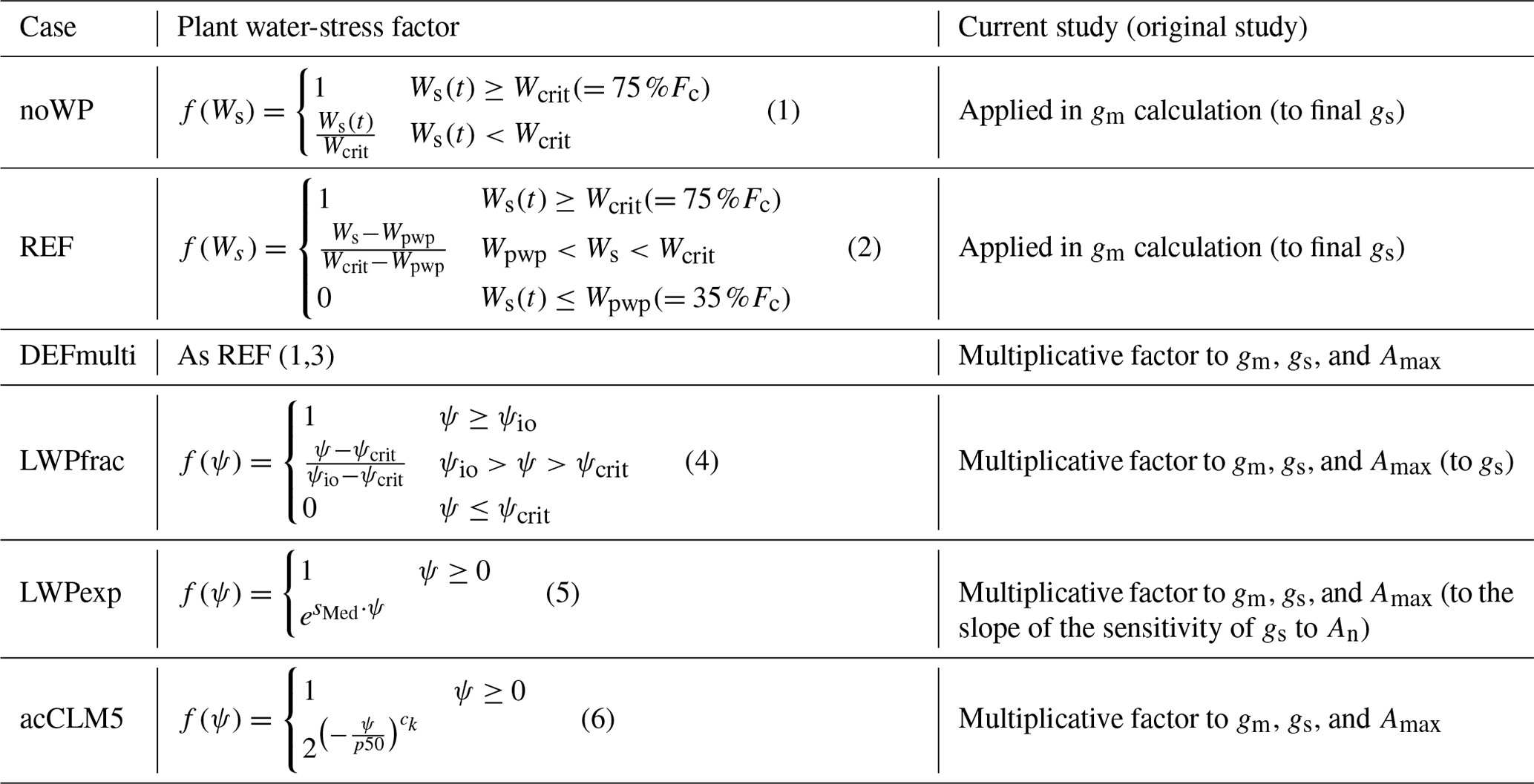
An overview of all parameterizations used as plant water-stress factors in the calculation of stomatal conductance is given in Table 1.

Table 1 Parameterizations for plant water stress used here, originally by (1) Schulz et al. (2001), (2) Delworth and Manabe (1988), (3) Verhoef and Egea (2014), (4) Zhang et al. (2003), (5) Sabot et al. (2022), and (6) acCLM5 (Kennedy et al., 2019), with g_m, g_s, and A_max being the mesophyll conductance, stomatal conductance, and maximum photosynthetic capacity, respectively. W_s, W_crit, and W_pwp are the actual soil wetness, critical soil wetness, and soil wetness at wilting point, respectively. F_c is the field capacity (maximum holding capacity of soil moisture). ψ, ψ_crit, and ψ_io are the actual leaf water potential, the critical value, and the value at final stomatal closure, respectively. The terms c_k, p50, and s_med are a vulnerability parameter, water loss at 50 % stomatal closure, and a sensitivity parameter, respectively.

2.1.4 Experimental design

We perform dynamical simulations with 3 h instantaneous and average output for each plant water-stress parameterization in the mesoscale (T106 = 1.12° or ≈60 km, middle atmosphere) for the period of 2017–2018. The dynamical simulations apply a set of sub-modules (AEROPT, CLOUD, CLOUDOPT, CONVECT, GWAVE, MSBM, OROGW, ORBIT, QBO, RAD, SURFACE, TROPOP, and VERTEX), similar to the setup used in Jöckel et al. (2016). The land–atmosphere exchange and vertical diffusion in EMAC are described here by the sub-model VERTEX (Emmerichs et al., 2021). The main functionalities of VERTEX are explained in Sect. 2.1.2. The warm-spell metric is calculated from a dynamical simulation at T42 (2.79° or ≈300 km), covering the period 1979–2008. To assess the impact on air pollution (see Sect. 3.5), we perform two chemical simulations (T106, 2017-2018). These simulations use additional sub-modules describing emissions of atmospheric species (OFFEMIS, ONEMIS, BIOBURN, and LNOX), gas exchange (DDEP and AIRSEA) and chemistry (MECCA and JVAL). The chemical mechanism includes the basic gas-phase chemistry of ozone, methane, and odd nitrogen with a total of 310 reactions and 155 species, as in Jöckel et al. (2016). The dry deposition of trace gases on vegetation is calculated according to the multiple resistance scheme, which uses the stomatal resistance calculated in VERTEX. The scheme is used here with six generalized land types. The vegetation canopy is represented as a single system; i.e. the detailed structure and plant characteristics are neglected (one big leaf approach). The leaves are oriented horizontally and the leaf density is uniformly distributed vertically (Kerkweg et al., 2006; Emmerichs et al., 2021). Further information regarding the sub-modules can be found in Jöckel et al. (2010, 2016). Two additional chemistry simulations comprise the CO₂ doubling experiments.

To reproduce the large-scale model dynamics (i.e the jet stream), the horizontal winds (divergence and vorticity) are nudged towards ERA5 reanalysis data by Newtonian relaxation applied as selective nudging for performing storyline simulations (Shepherd et al., 2018). This allows the model thermodynamics to respond freely to the process modifications implemented in this study.

2.2 Observational data

2.2.1 EUMETSAT

Evapotranspiration observations have been provided by the European Organisation for the Exploitation of Meteorological Satellites (EUMETSAT) using the second generation of geostationary Meteosat satellites. This covers the area of Europe, Africa and most of South America, with a spatial resolution of 3 km. The Spinning Enhanced Visible and Infrared Imager (SEVIRI) radiometer operating (among others) on board provides the surface radiation component. These data, other biophysical parameters, soil moisture data from remote sensing, recent land cover information from the ECOCLIMAP land cover database, and meteorological fields from numerical weather prediction drive a physical model of the energy exchange in the soil–vegetation–atmosphere system. According to this, the flux [mm h⁻¹] of water evaporated at the earth–atmosphere interface (soil, vegetation, and water bodies) and transpired by vegetation through stomata (as a consequence of photosynthetic processes) is calculated within a soil–vegetation–atmosphere transport model (SVAT; EUMETSAT, 2018):

$$\begin{array}{}\text{(9)}& {\displaystyle }\begin{array}{rl}{\displaystyle }& {\displaystyle }\text{ET}=\mathrm{3600}{\displaystyle \frac{{\text{LH}}_{\mathrm{T}}}{L_{\mathrm{v}}}},\\ {\displaystyle }& {\displaystyle }{\text{LH}}_{\mathrm{T}}={\displaystyle \frac{L_{\mathrm{v}}\mathit{\rho }}{(r_{\mathrm{a}}+r_{\mathrm{s}})}}\left[q_{\text{sat}}\right({\text{temp}}_{\mathrm{s}})-q_{\mathrm{a}}({\text{temp}}_{\mathrm{a}}\left)\right],\end{array}\end{array}$$

where LH_T is the latent heat flux of transpiration [W m⁻²], L_v the latent heat of water vapour [J kg⁻¹], ρ the air density [kg m³], r_a and r_s the aerodynamic and stomatal resistances (inverse of the conductance), q the specific humidity, and q_sat(T_s)−q_a(T_a) the atmospheric saturation deficit [kg kg⁻¹]. These products have been downloaded from the website of the EUMETSAT Land Surface Analysis (LSA SAF) consortium website (https://user.eumetsat.int/catalogue/EO:EUM:DAT:MSG:DMET, last accessed: 29 June 2023) with a time interval of 3 h (original frequency – 30 min). For comparison with the model results, the downloaded dataset was regridded to the EMAC spatial grid. The product validation report found a general accuracy of 20 %–25 %, which is equivalent to the accuracy of measurements. The main uncertainties may be due to the physical formalism of the algorithm, the errors in the input data, surface heterogeneity, and sensor performance, among other uncertainties (EUMETSAT, 2018).

2.2.2 GLEAM

The Global Land Evaporation Amsterdam Model (GLEAM) estimates the evaporative flux over land by assimilating satellite observations. Land evapotranspiration is the sum of the bare soil, short vegetation, and tall vegetation in each grid box. The soil water content of several layers (depending on the land type) is calculated as a water balance between the input snowmelt and rainfall (minus interception). Surface soil moisture observations from satellites are assimilated (using the Kalman filter approach) at a daily time step based on their uncertainty. The Priestley–Taylor equation calculates the potential latent heat flux λE_p [MJ m⁻²] using

$$\begin{array}{}\text{(10)}& \mathit{\lambda }{E}_{\mathrm{p}}=\mathit{\alpha }{\displaystyle \frac{\mathrm{\Delta }}{\mathrm{\Delta }+\mathit{\gamma }}}(R_{\mathrm{n}}-G)\end{array}$$

as a function of the net radiation (R_n, daily observations) and the ground heat flux (G). Δ is the slope of the temperature/saturated vapour pressure curve ([k Pa K⁻¹]). Division by the latent heat of vaporization λ gives the potential evaporation (E_p [mm]). For optimal environmental conditions, α=0.8 and α=1.26 are used for tall and short vegetation (or bare soil), respectively. An evaporative stress term (S) is used to convert E_p to actual transpiration (T [mm d⁻¹] from vegetation):

$$\begin{array}{}\text{(11)}& T=S{E}_{\mathrm{p}}.\end{array}$$

S is parameterized separately for tall and short canopy and for bare soil (then Eq. 11 yields bare soil evaporation) based on the observed soil moisture conditions and optical depth of vegetation. Canopy interception loss (I) is estimated in a separate module based on observations of daily precipitation; snow depth; tall canopy fraction; lightning climatology; and parameters for canopy cover, canopy storage, mean precipitation, and evaporation rate under saturated canopy conditions. The use of an interception loss fraction (β=0.007) ensures that wet canopy evaporation is only considered once in the calculation. An additional module estimates the snow and ice sublimation for the snow-covered pixels (no stress) where α=0.95. Evaporation from lakes and rivers is not included. More details can be found in Miralles et al. (2011). The data have been downloaded from the ftp server after registration (https://www.gleam.eu/#downloads, last access: 24 July 2023).

2.2.3 TROPOSIF

Solar-induced chlorophyll fluorescence (SIF) can be observed using remote sensing. This is an electromagnetic signal emitted by the chlorophyll of assimilating plants that is not used for photosynthesis. This can be a proxy for photosynthetic activity, as the SIF signal is sensitive to perturbations caused by environmental stress (Maes et al., 2020). However, the estimation requires high spectral resolution and advanced retrieval schemes since the emissions contribute only a small fraction of the radiance. The TROPOMI (TROPOspheric Monitoring Instrument) instrument on board the Copernicus Sentinel-5 Precursor satellite launched in October 2017 measures top-of-the-atmosphere radiance. This is fitted in the far-red spectral region by inverting a linear forward model. SIF estimates from the 743–758 nm window are the most robust to atmospheric effects such as cloud contamination. The L2B product used here (the SIF dataset from TROPOMI – TROPOSIF) combines all observations at the individual orbits into an un-gridded netCDF4 file (NOVELTI et al., 2021). Evaluation against other SIF products showed a general consistency in terms of level and amplitude of the retrieved SIF and seasonality for vegetated surfaces. The indicative error threshold for the definition of spatiotemporal bins is 0.2 $\mathrm{mW}{\mathrm{m}}^{-\mathrm{2}}{\mathrm{steradian}}^{-\mathrm{1}}{\mathrm{nm}}^{-\mathrm{1}}$ (about 10 % of the globally observed peak SIF values; Guanter et al., 2015). This corresponds to 0.064 mm d⁻¹ of transpiration. In addition, the data product includes a quality flag that is used here for individual quality assurance. The data can be downloaded from http://ftp.sron.nl/open-access-data-2/TROPOMI/tropomi/sif/v2.1/l2b/ (last access: 5 November 2023) (NOVELTI et al., 2021; Guanter et al., 2015). According to Maes et al. (2020), SIF can be converted to the latent heat flux of transpiration (LH_T [W m⁻²]) using

$$\begin{array}{}\text{(12)}& {\text{LH}}_{\mathrm{T}}=\mathrm{61.4}\cdot \text{SIF}.\end{array}$$

Using the latent heat of water vapour ($L_{\mathrm{v}}=\mathrm{1.5}\times {\mathrm{10}}^{\mathrm{6}}$ [J kg⁻¹]) gives the transpiration [mm d⁻¹]:

$$\begin{array}{}\text{(13)}& T={\text{LH}}_{\mathrm{T}}/L_{\mathrm{v}}\cdot \mathrm{3600}.\end{array}$$

To compare this dataset to the EMAC model, we sample the instantaneous output along the satellite orbit at 13:30 UTC.

3 Results and discussion

3.1 Plant water stress and transpiration

The stress functions summarized in Table 1 result in a variety of different plant water stresses and thus values for transpiration. Figure 1 gives a first overview of how the response functions vary with proxies for water stress (soil moisture and leaf water potential). Decreasing “volumetric” soil moisture (soil wetness divided by the field capacity) linearly increases plant water stress for the REF and DEFmulti cases (black line) until the wilting point (35 % of the field capacity) is reached. Using the noWP function (grey line), plants experience a lower level of stress as the soil dries, but this can increase to the point of stomatal closure (stress factor = 0). The LWPfrac and acCLM5 functions mostly show a linear increase in the stress with increasing water demand (more negative ψ). The acCLM5 function also covers the ψ range between 0 and −1 [MPa] where the response is much weaker. LWPexp is a simple exponential function with a steep increase in the stress response for ψ between 0 and −1 [MPa]. In comparison, Verhoef and Egea (2014) observed a sigmoidal dependence on soil water for most plant water stress in most plant species (their Fig. 1). The recent modelling study by Harper et al. (2021) used a function with a simple quotient depending on soil moisture similar to the functions REF and DEFmulti. They obtained model improvements by replacing soil moisture with the soil matrix potential, for which ψ (used in LWPfrac) can be used as a proxy (Kozlowski et al., 1991; Verhoef and Egea, 2014). Early observations of increasing stomatal conductance with increasing ψ (to lower negative values; see Fig. 2b in Sellers et al., 1997) are generally consistent with these results.

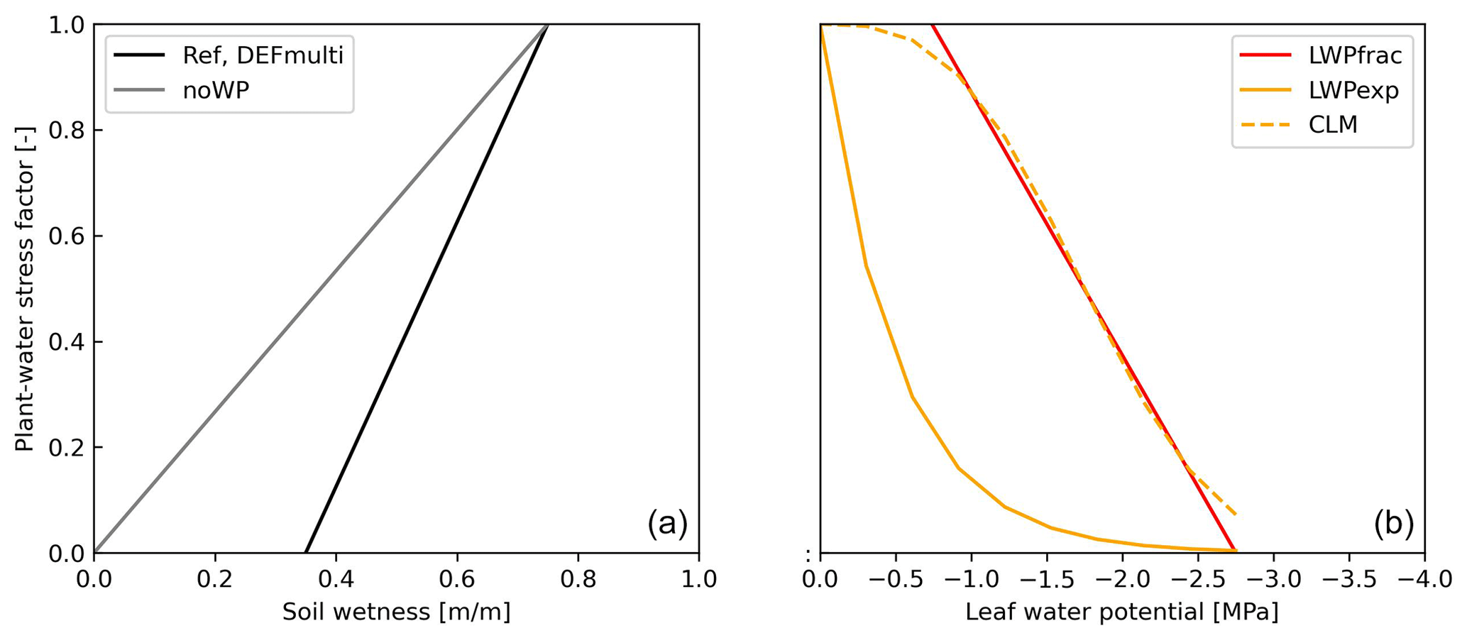
Figure 1 Plant water stress factor vs. (volumetric) soil wetness (a) and leaf water potential (b) of the parameterizations indicated.

Figure 2 shows the simulated annual mean maximum photosynthetic capacity (A_m,max) and transpiration (T) and their changes. The global distribution (simulated by REF) follows the spatial distribution of air temperature and CO₂ concentration in the leaf stomata. A_m,max is strongly driven by leaf (2 m) temperature, as shown in Fig. 2a. Until the stomatal conductance is upscaled to the canopy level (see ECMWF, 2021, Eq. 8.123), the intermediate calculations, e.g. for A_m,max, are at the leaf level. Thus, the distributions over non-vegetated areas such as the Sahara Desert are masked out here (vegetation fraction > 1 %), which depends on the modelled vegetation mask. Transpiration (Fig. 2b) also depends on atmospheric moisture, which explains its maxima in tropical rainforests. Multiple applications of the default stress factor (to g_m, A_m,max, g_s; DEFmulti) lead to small decreases in A_m,max (Fig. 2c) in dry areas (SM<W_pwp, soil moisture limited). Thus, transpiration is not significantly altered (Fig. 2d, max=0.5).

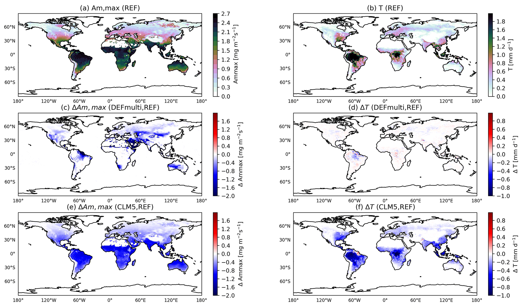
Figure 2 Annual mean maximum CO₂ assimilation rate (A_m,max) (a), transpiration (T) (b), and the respective changes to DEFmulti (c, d) and acCLM5 (e, f), masked for vegetated region (vegetation fraction > 1 %).

The effects of the plant water-stress functions based on leaf water potential (e.g. LWPfrac) are more widespread in vegetated areas, as the parameterization is temperature driven. A_m,max (Eq. S2 in the Supplement) and also the daily transpiration decrease significantly by 1–2 mm d⁻¹, which is highest in the tropical rainforest (Fig. 2f). This can be explained by the radiation maximum in the inner tropics. Therefore, the 30 % increase in plant water stress and the subsequent decrease in maximum photosynthetic capacity and mesophyll conductance (not shown here) have a greater influence in the tropics compared to other regions on the SH continents (Fig. 2e). With the onset of the boreal summer in May/June, the influence spreads to Europe and the USA, while it is limited to the evergreen tropical forests in the SH. The changes in the sensitivity simulations LWPexp and acCLM5 (not shown here) have the same spatial distribution. In the regional plots (Fig. 3), there is only a small difference between the changes in plant water stress and the subsequent variables. Thus, the linear and exponential formulations can be interpreted in a similar way. All three stress functions based on leaf water potential (LWPfrac, LWPexp, acCLM5) introduce an additional dependence of the modelled transpiration on air temperature (except in arid climates). In fact, this slows down the increase in transpiration with increasing temperature. Accordingly, the amplitude of the diurnal cycles decreases (Fig. 3). On the other hand, the diurnal cycle of plant water stress initially shows variations, which is an observed phenomenon according to Xiao et al. (2021). In contrast to LWPfrac and acCLM5, which predict not only the same ψ but also the same f(ψ), LWPexp estimates a higher (negative) ψ in most regions (shown in Fig. 3). This can be explained by the temperature–transpiration feedback expected in arid climates (the Arabian Peninsula and the African savannah). In addition, the simple exponential function in LWPexp gives a stress factor close to zero and thus unrealistically shuts down the mesophyll conductance and the photosynthetic activity, unlike LWPfrac and acCLM5. Analysis of the noWP and DEFmulti simulations shows only small local changes in transpiration (within the monthly variance range), affecting the annual estimate by only ±10 %–15 %. This is because neglecting the wilting point reduces plant water stress ($f_{W_{\mathrm{s}}}$) by only 10 % in all dry vegetation regions (dry climate – $W_{\mathrm{s}}<\mathrm{0.35}\cdot F_{\mathrm{c}}$; see Seneviratne et al., 2010) and thus transpiration is only marginally affected.

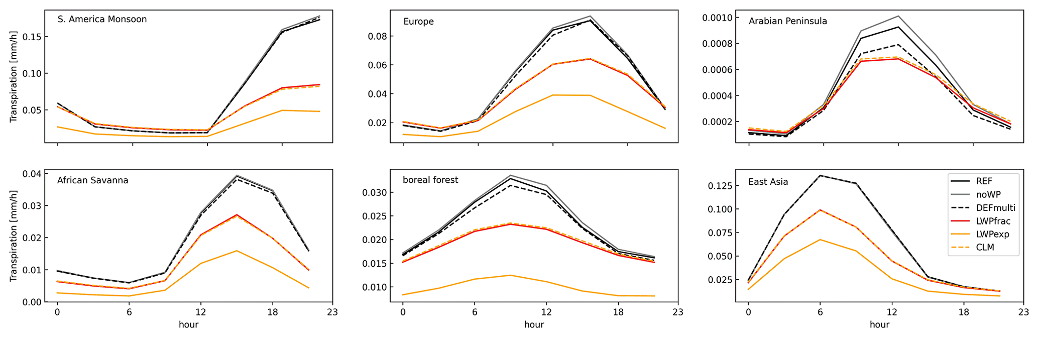
Figure 3 Regional mean diurnal cycle of transpiration in the South American monsoon region, Europe, the Arabian peninsula, the African savannah, boreal forest, and east Asia in boreal summer. The regions are defined in the respective order by the following scientific regions: 12; 16–18; 36, 21; 18, 29, 30, 31, 2, 1; and 35 according to the Intergovernmental Panel on Climate Change (IPCC) reference definitions (Iturbide et al., 2020).

3.2 Global estimates of transpiration

All EMAC simulations show a realistic spatial variation in annual transpiration (Fig. 2b). However, the low variance ratio (VR) values globally (Table 3) indicate that the simulated variability is lower (VR<1) compared to the GLEAM dataset. This cannot be attributed to an oversimplification of the modelled process. GLEAM is based on the Priestley–Taylor equation, an empirical equation dependent on solar radiation and temperature, compared to the physically based Penman–Monteith approach used in EMAC (Table 2). The EMAC reference simulation with the standard plant water stress overestimates the global mean transpiration calculated with GLEAM by 46 mm yr⁻¹ (16 %; Table 3), which is well within the uncertainty range of the GLEAM product (±136 mm yr⁻¹). The LWPfrac and acCLM5 stress factors correct this overestimation regionally. The new global (mean) model estimate of 276 and 277 mm yr⁻¹ is lower than the GLEAM estimate. Compared to the GLEAM uncertainty, all model simulations show a higher 1σ (standard deviation) range, indicating a higher uncertainty, which could, for example, be due to the representation of precipitation in the model. In GLEAM, however, precipitation is derived from satellite observations (see Sect. 2.2.2). A lower 1σ in the sensitivity simulations based on the leaf water potential indicates an improvement due to the neglect of the uncertain soil moisture data usually used in the model. The use of the transpiration estimate from the TROPOSIF data gives a good comparison with the (monthly mean) model predictions (only a small underestimation) over areas with high transpiration (e.g. Europe and east Asia) in spring and late autumn. Under strong drought conditions, solar-induced plant fluorescence decouples from transpiration (Maes et al., 2020), and thus the linear relationship between SIF and T (applied here) is no longer valid, e.g. during the boreal summer (Martini et al., 2022). However, compared to GLEAM (masked for the TROPOSIF region), the TROPOSIF dataset predicts lower daily transpiration in spring and higher transpiration in autumn. The seasonality of SIF strongly follows the growing season in the NH, which may cause some discrepancies.

Table 2 Formulae for plant transpiration and evapotranspiration from EMAC and the observational datasets used.

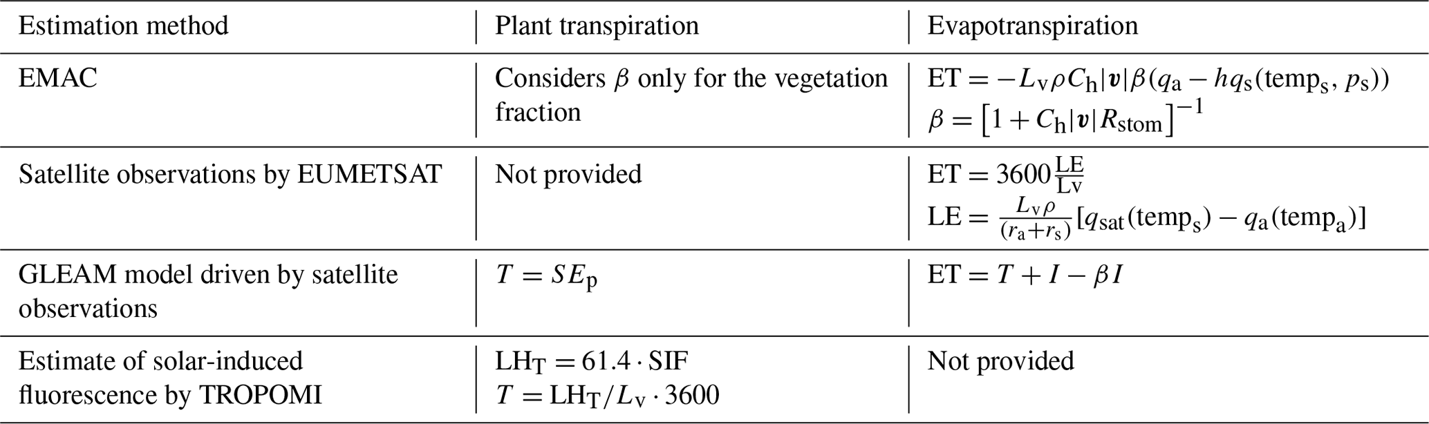
Table 3 The global estimates of transpiration (1σ – standard deviation), normalized absolute error (NAE), and the variance ratio (VR; $\frac{\text{var(mod)}}{\text{var(obs)}}$), accounting for grid boxes with more than 1 % vegetation.

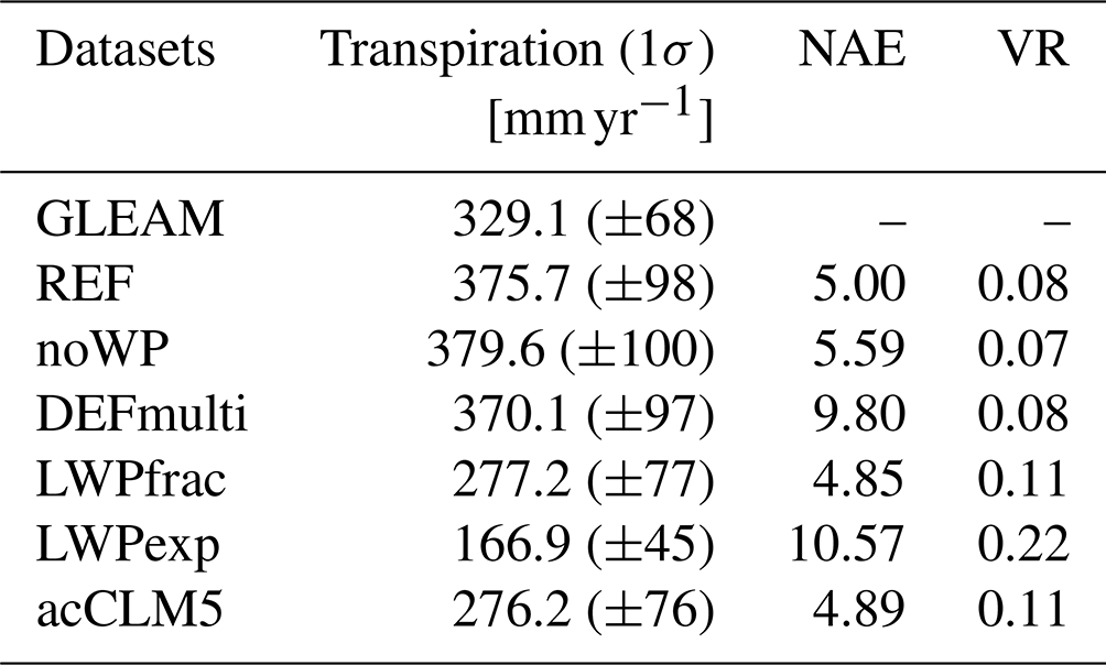
Taking into account the multi-model ET estimate from 18 CMIP6 models (1980–2014; ET grows with time) and the observation-based $T/\text{ET}$ ratio of 64 % from Pan et al. (2020), an estimated global transpiration of 384 mm yr⁻¹ is obtained. It can be concluded that all model estimates in our study predicted annual transpiration reasonably well. The only exception is the sensitivity simulation LWPexp, which shows an unrealistically large reduction and thus a high normalized absolute bias (NAE), probably due to the choice of constraining parameters (see Eq. 7). For further impact assessments in this study, we use the stress factor LWPfrac as it performs best overall (slightly better than the acCLM5 factor).

3.3 Contribution to global evapotranspiration

The contribution of transpiration to the total ET varies in time and space with vegetation and soil characteristics (Wang and Dickinson, 2012; Cao et al., 2022; Lian et al., 2018). This spatial variability is reflected in GLEAM and EMAC, where the estimates are particularly inconsistent in Europe and Africa (Fig. 4). Lian et al. (2018) report the dominance of soil evaporation over transpiration in arid (non-vegetated) regions. This is also shown in our study in the Sahara Desert by a low $T/\text{ET}$ ratio (in GLEAM and EMAC) and in non-vegetated parts of China (EMAC). Similarly, the low $T/\text{ET}$ ratio in the northernmost (partly snow-covered) areas of Canada and Siberia (as shown in Lian et al., 2018) is only captured by EMAC (not by GLEAM). In humid regions, especially in the tropics, evapotranspiration is driven by transpiration. The contribution can be up to 87 % over densely vegetated regions. Observations in the Amazon tropical forest indicate an average $T/\text{ET}$ ratio of 0.7 (Wang and Dickinson, 2012; Zhang et al., 2017). This can be consistently represented by EMAC (Fig. 4b), although the sensitivity simulations, e.g. LWPfrac and acCLM5, partly reduce the $T/\text{ET}$ ratio too much in southern Argentina (Fig. 4c and d). According to the simulated and observational estimates of $T/\text{ET}$ by Lian et al. (2018, their Fig. 1a), all EMAC simulations represent too-low values in most parts of the USA, suggesting a dry model bias. For the central USA, Dong et al. (2022) indeed confirm that unbiased estimates of summertime daily maximum temperature can only be achieved with a $T/\text{ET}$ ratio of 0.7. In contrast, GLEAM shows higher values of the $T/\text{ET}$ ratio for the east coast of the USA, as well as for the SH continents, Europe, and Asia. Incorrect E–T partitioning has been identified as a source of error in ET estimation in CMIP5 models (Lian et al., 2018).

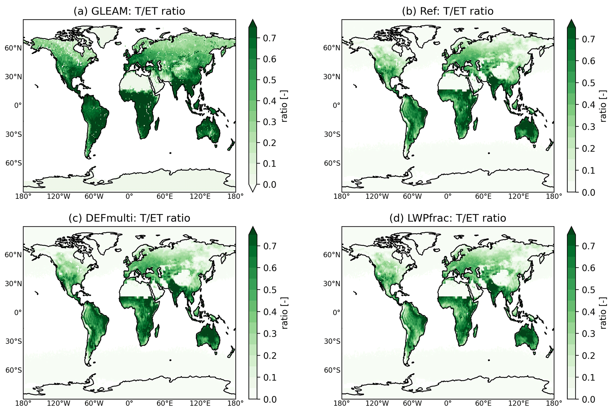
Figure 4 Annual mean ratio of transpiration:̇ evapotranspiration by (a) GLEAM, (b) REF, (c) DEFmulti, and (d) LWPfrac in 2018.

To assess the model estimation of evapotranspiration, we compare it with ET estimates from GLEAM and EUMETSAT. GLEAM generally gives higher estimates (Fig. 5a and c). ET has its maximum in the tropics, while in the high northern latitudes and sparsely vegetated areas (e.g. the Sahara Desert), low values occur. The GLEAM estimate (for the EUMETSAT region) of ET (512 mm yr⁻¹) differs by 30 mm yr⁻¹ (6 %) from the EUMETSAT value (481 mm yr⁻¹), which could be considered within the uncertainty range. However, the difference can be large regionally, by as much as 50 %. This is most evident in the tropics and consistent with recent studies. Compared to the literature values by Elnashar et al. (2021), who calculated an annual ET of 540 mm yr⁻¹ (for 2018), the GLEAM estimate is the most consistent. Thus, the models usually differ by 200 mm yr⁻¹, which is about twice the spread of estimates by single models (minima and maxima; Wang et al., 2021). In a model intercomparison, Pan et al. (2020) report a large spread and a high uncertainty in model estimates for ET at low latitudes due to the parameterization of root water uptake.

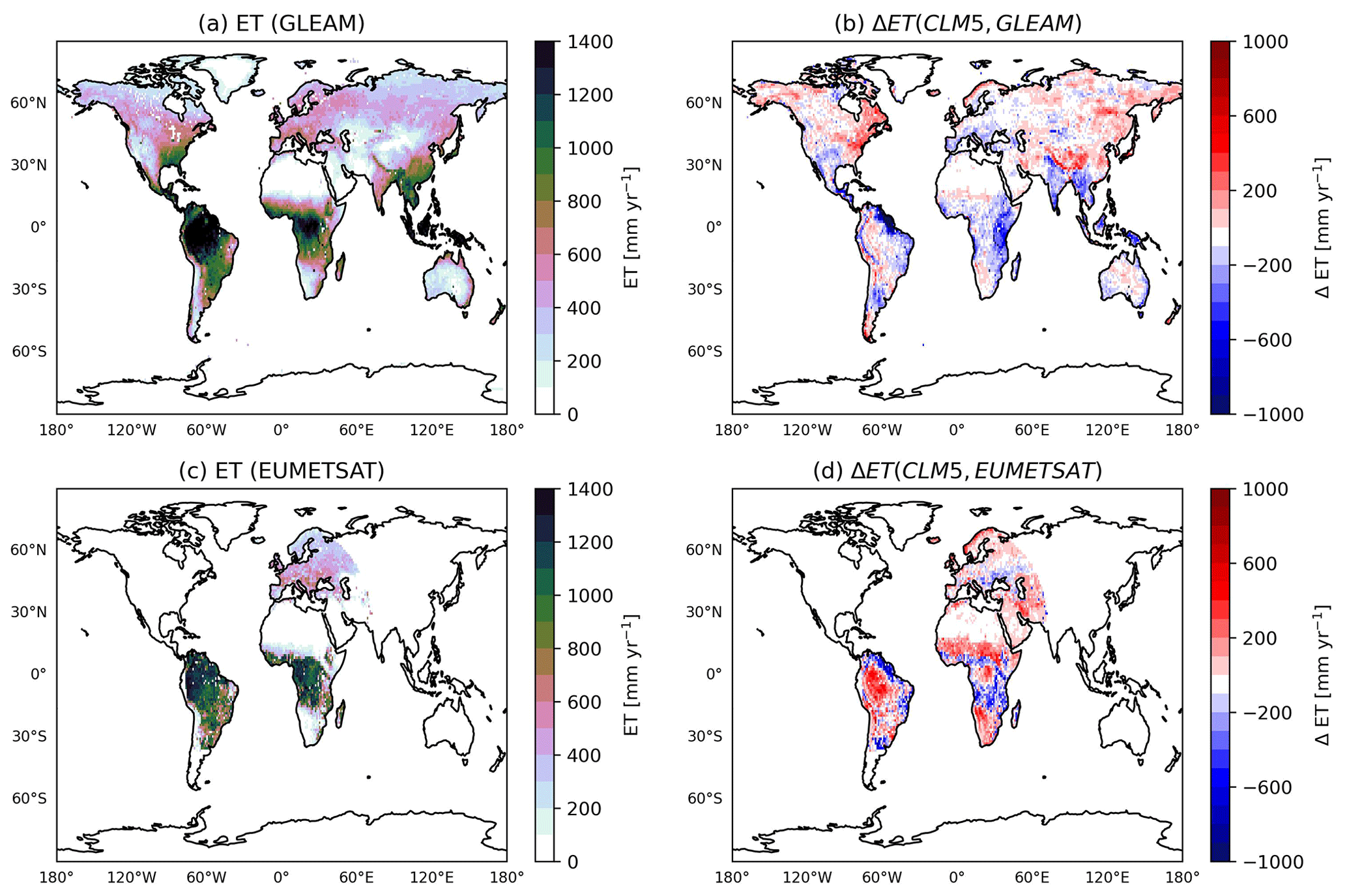
Figure 5 Annual mean evapotranspiration (ET) of (a) GLEAM and its difference to (b) the acCLM5 sensitivity simulation (acCLM5-GLEAM) (c) Annual evapotranspiration (ET) of EUMETSAT and (d) its difference to the acCLM5 sensitivity simulation.

The global average of annual ET predicted by EMAC with the different plant water-stress parameterizations is about 425–480 mm yr⁻¹. The ET predicted by the acCLM5 sensitivity simulation, which best reproduces transpiration (see Sect. 3.2), compares well with the GLEAM annual values. Especially in some coastal areas, such as in the eastern USA and the northeastern Amazon, there are significant differences, which could be due to neglected sub-scale coastal hydrology (Fig. 5b). Compared to EUMETSAT, EMAC (as well as GLEAM) estimates a higher annual mean ET in tropical rainforests, while in tropical monsoon climate regions it simulates too-low values compared to EUMETSAT (Fig. 5d). This pattern of differences points to precipitation as the cause, since these two climate types differ mainly in the amount of precipitation. This result is consistent with the known precipitation bias of the ECHAM5 climate model (see Fig. 7 in Stevens et al., 2013). Both EMAC and EUMETSAT underestimate the global GLEAM ET, with more than 50 % of the discrepancy occurring outside the EUMETSAT region. The difference cannot always be considered to be within the model variability of 20 %. As a possible reason for the large variability, we propose the model net radiation, which depends on the choice of forcing data (Badgley et al., 2015). One reason for the underestimation is probably neglect of the effect of diffuse radiation in big-leaf models, such as the one used here. Including diffuse radiation would increase photosynthesis and evapotranspiration (Wang et al., 2022; Knohl and Baldocchi, 2008). Furthermore, the representation of deep plant roots would ensure a more realistic water-holding capacity and avoid soil desiccation in tropical rainforests (Hagemann and Stacke, 2015).

3.4 Impact on air temperature

The changes in ET have a significant effect on the air temperature. Here, we compare the temperature predicted by REF to that predicted by LWPfrac. As expected, a decrease in ET, i.e. less cooling, leads to an increase in high daily maximum air temperature values, shown in Fig. 6 for warm spells in 2018. We define a warm spell as a period of at least 3 consecutive days when the daily mean temperature exceeds the 95 % percentile of the daily mean temperature for the reference period (1979–2008; Nairn and Fawcett, 2014). In fact, the difference between the actual temperature and the climatological percentile, which is a measure of intensity of warm spells and is called the “excess heat factor” in Nairn and Fawcett (2014), increases by 1.5 K in Europe and 4 K in South Africa, in the eastern US, and in the Amazon forest due to the changed plant water-stress function of LWPfrac. The global mean air temperature in the lowest model layer (≈60 m) increases by 2 K. These results are consistent with recent studies (e.g. Seneviratne et al., 2010; Kala et al., 2016), which highlight the role of stomatal stress in the amplification of heat waves, especially with respect to their intensity (Barriopedro et al., 2023).

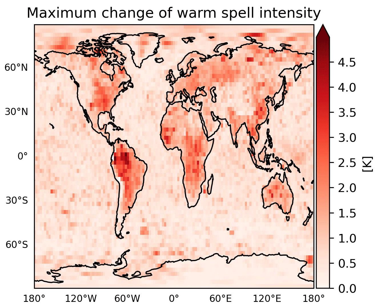
Figure 6 The maximum annual change in warm-spell intensity (difference in the actual temperature to the climatological percentile) in 2018 due to the plant water-stress function.

3.5 Impacts on air pollution

The different representations of plant water stress affect air pollution mainly by influencing (1) dry deposition fluxes of ozone and (2) meteorological controls on photochemistry. Figure 8 shows the effects on tropospheric ozone (O₃) when using the LWPfrac plant water stress. Figure 8a shows that the dry deposition of O₃ in LWPfrac is reduced by up to 25 % compared to REF in the tropics and subtropics, where dry deposition exerts a strong control on air composition due to high vegetation density. Similar changes apply to precursors with similar characteristics as O₃. This contributes to the increase in the O₃ mixing ratio (Emmerichs et al., 2021). Furthermore, the reduced ET in most vegetated regions exacerbates the atmospheric moisture deficit, which places additional stress on the stomata. The increased plant water stress leads to a significant temperature increase throughout the tropical regions (see previous section), which is known to favour O₃ production (Pusede et al., 2015). However, the annual mean chemical production and loss terms (Fig. 8b and c) are increased only in the southwest of South America (by up to 10 %). The increase in O₃ production shown here follows the increase in OH and HO₂ (HO_x) production. Plant emission activity as modelled by the MEGAN model (Model of Emissions of Gases and Aerosols from Nature) increases with higher temperature up to a value of approximately 40 °C (Guenther et al., 2006). The increasing emissions lead to a linear increase in O₃. As shown in Fig. 7a and b for the Amazon, O₃ increases by 0.34 ppb per 1 ppb increase in formaldehyde (HCHO). HCHO is a direct product of isoprene oxidation with a lifetime of a few hours and is therefore often used as a proxy for isoprene emissions (Palmer et al., 2003). Rapid oxidation reduces C₅H₈ and increases OH surface concentration in the inner tropics (the Amazon and the Congo basins; Fig. S1). In the outer tropics, O₃ additionally increases with increasing soil emissions of nitrogen oxides (NO), which are an important O₃ precursor source in remote regions (far from anthropogenic emissions). The change in O₃ loss is of the same magnitude but more widespread than the change in O₃ production, driven by a relative acceleration of NO_x and HO_x chemistry. These effects then lead to an increase in net O₃ loss in the Amazon basin, which is overcompensated for by a decrease in O₃ uptake by vegetation. Thus, the annual mean surface O₃ in the tropics and subtropics is increased by up to 10 % (Fig. 8d). This increases the global tropospheric O₃ burden by 5 Tg yr⁻¹.

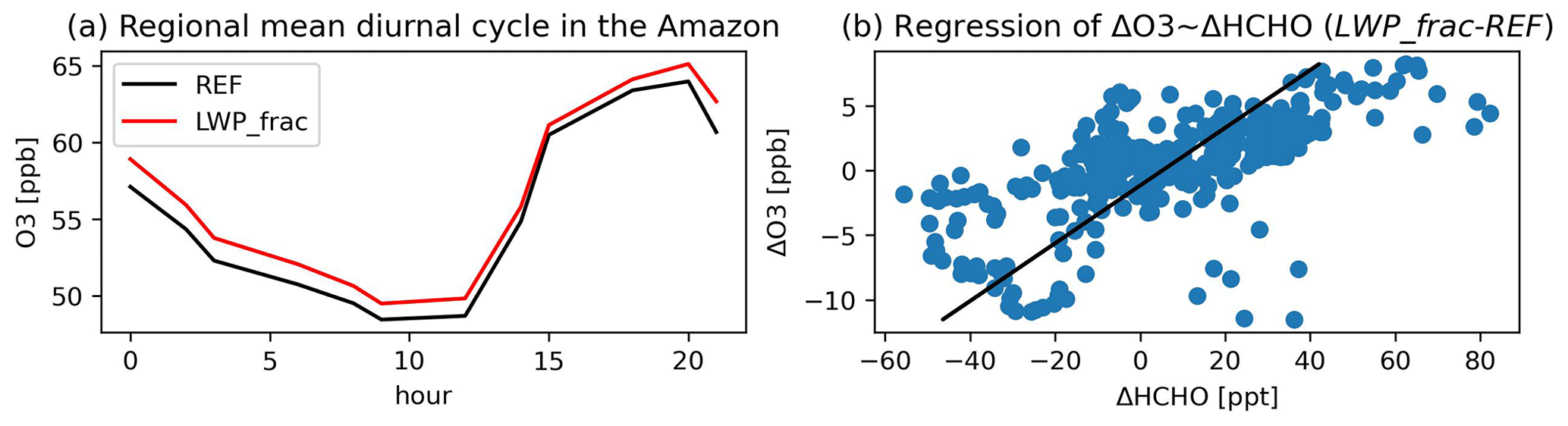
Figure 7 (a) Regional mean diurnal cycle of O₃ in the Amazon (monsoon region, definition in Fig. 3) and (b) linear regression of the absolute difference (LWPfrac-REF) in formaldehyde (HCHO) with O₃ surface levels at the ATTO (Amazon Tall Tower Observatory) site in November 2018 (dry season).

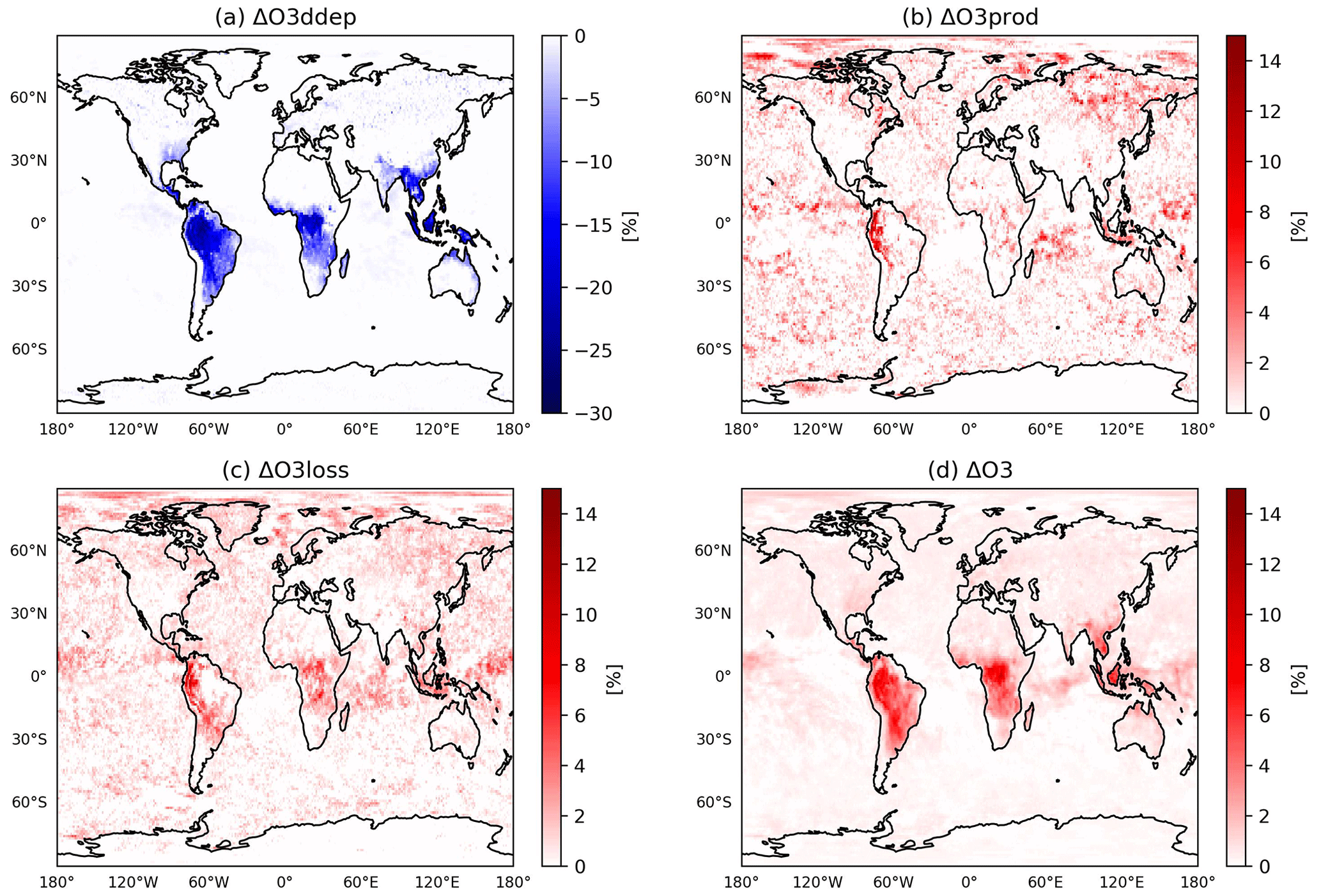
Figure 8 The relative change between LWPfrac and REF of the annual mean (a) O₃ dry deposition, (b) chemical O₃ production, (c) chemical loss, and (d) surface O₃ mixing ratio.

The changes discussed here do not include the O₃ damage to plants, i.e. the biosphere–atmosphere exchange. However, from experiments by, for example Sadiq et al. (2017), we can learn that implementation of this response amplifies the O₃–vegetation feedback because the O₃-increase caused increasingly damages the plant cells and limits their activity. This further reduces the transpiration and dry deposition, which in turn increases O₃ levels. No clear feedback was found for isoprene emissions. Reduced ecosystem production makes only a small contribution to the overall feedback.

3.6 Future scenario

A simulation with the double CO₂ concentration (futureLWPfrac) was performed to investigate the role of the new plant water-stress factor in future climate conditions. In addition to perturbing the energy balance at the top of the atmosphere, CO₂ affects the sensitivity of plants to water stress in our simulations. An increase in CO₂ has two effects on plant behaviour. While it leads to increased photosynthetic activity, the stomatal conductance is reduced by an average of 40 % (g_s; Fig. 9a). Vicente-Serrano et al. (2022) report a decrease of 22 % in stomatal conductance (on average) from multiple experiments by doubling only CO₂. We can also confirm these findings for equatorial and tropical forests in our simulation. Due to the dominant decrease in g_s, as also reported by Vicente-Serrano et al. (2022), plant transpiration decreases in response to increasing CO₂ in these regions. In our simulations, however, the impact of the future conditions on g_s is more widespread, as the increased CO₂ also reduces relative humidity almost worldwide, thus stressing plants. The 30 % decrease in g_s associated with the new plant water-stress function is amplified by the enhanced CO₂. However, this dominates the ET on a daily basis only, while the annual sum increases by 30–100 mm yr⁻¹ in response to increased evaporative demand. As a consequence, the 2 m temperature increases by up to 3 K (Fig. 9b), and the relative humidity decreases (not shown). These changes are associated with the 20 %–50 % increase in solar irradiation (correlation) due to fewer low-level clouds. Pollard and Thompson (1995) also report a doubling CO₂ scenario that leads to an increase in stomatal conductance, temperature, and specific humidity and thus to a decrease in relative humidity and cloudiness. ECHAM/MESSy does not simulate an interactive carbon cycle; instead photosynthesis, i.e. the net assimilation of CO₂, is calculated to simulate the stomatal conductance with a first-order dependence scaled by the CO₂ deficit between plant cavity and the atmosphere. Several studies have reported that an increase in atmospheric CO₂ reduces the leaf stomatal conductance by 50 % in dense meadows, by 15 % in deciduous forests, and by less than 10 % in coniferous forests. This response is non-linear because the CO₂ stimulation of photosynthesis saturates at high atmospheric CO₂ (Vicente-Serrano et al., 2022, and references therein). Nevertheless, to assess the overall climatic impact of the multiple interactions between terrestrial vegetation and CO₂, the changing vegetation would also have to be taken into account. However, such an assessment is far more complex and highly uncertain (Vicente-Serrano et al., 2022).

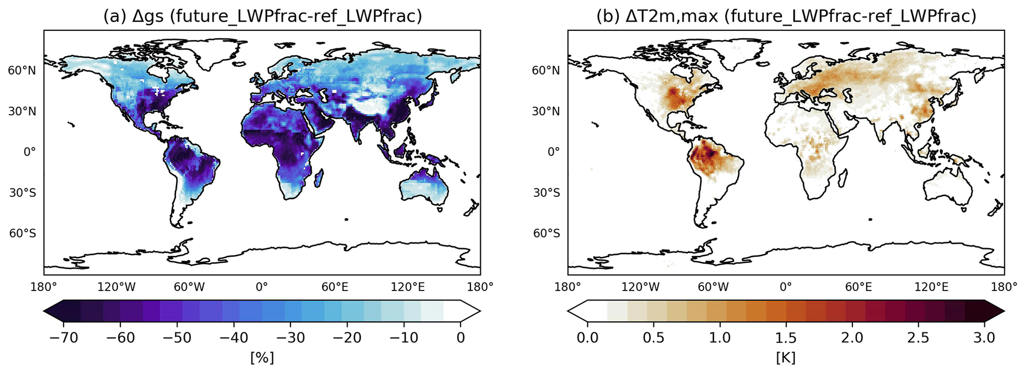
Figure 9 The (boreal) summer mean change in stomatal conductance (a) and daily 2 m maximum temperature (b) when comparing LWPfrac for normal and future conditions (double CO₂).

4 General discussion

4.1 Default model parameterization

In models, ET is estimated using either the physically based Penman–Monteith (PM) approach (state of the art) or the empirical Priestley–Taylor (PT) equation. The latter (used in GLEAM) assumes that ET depends only on solar radiation and temperature, neglecting wind speed, relative humidity, and vapour pressure deficit. However, because of the link with air temperature, estimates from the PT approach show a high correlation with values estimated by the PM equation, which are expected in dry conditions and in areas with relatively high wind speed (Utset et al., 2004). The key variable for the common parameterization of water stress in plants is soil moisture, which is described in EMAC by the simplistic but conventional bucket model. A bucket model has long been used, for example, in the JSBACH (Jena Scheme for Biosphere Atmosphere Coupling in Hamburg version) land surface model (Boone et al., 2004). The inclusion of the surface resistance term in EMAC as a so-called “second-generation model” allows a better comparison of estimated evapotranspiration rates with observations than the use of “pure” bucket models does (Sellers et al., 1997). However, the lack of soil water holding capacity in the (shallow, one-layer) bucket model leads to an immediate removal of water and thus to unrealistically low soil water in areas with deep roots, e.g. tropical forests (Hagemann and Stacke, 2015), despite the thickness of the subsurface layers. Nevertheless, the multi-model evaluation by Robock et al. (1998) found no significant improvements over the bucket scheme in sophisticated soil models with multiple layers and even in vegetation dynamics such as the CLM or NOAH-LSM. More recently, Dong et al. (2022) concluded that most CMIP6 models simulate a warm bias in mid-latitude summer due to incorrect partitioning of ET in canopy transpiration and soil evaporation due to shallow soil. In addition, even small differences in the input field capacity data can have large effects on the simulated ET (Hagemann and Stacke, 2015).

4.2 More sophisticated models, remaining uncertainties, and future recommendations

Boone et al. (2004) show that sophisticated land surface models (LSMs) generally agree with respect to latent heat flux and total runoff. However, we note that it is very difficult to compare different LSMs because of differences in model components, parameterization, and choice of associated parameters. In addition, many LSMs only represent shallow soils with a maximum depth of 2 m (Pan et al., 2020) and therefore cannot account for the storage capacity of soils in tropical forests as shown by Hagemann and Stacke (2015). The second-generation LSMs Pitman (2003), which calculate transpiration and soil moisture over multiple layers, predict soil moisture slightly better than the bucket model. However, LSMs show a wide range of performance compared to observations (Shao and Henderson-Sellers, 1996). This is certainly due to but not limited to the use of different schemes for simulating surface fluxes and soil moisture. In general, the required spinup time of LSMs with deep soil schemes is often not affordable, especially for climate simulations. The use of an additional groundwater model (e.g. Jiang et al., 2009; Kollet and Maxwell, 2008; Lam et al., 2011; Larsen et al., 2014) can improve the simulation of the water balance and the groundwater–land surface interactions (Rahman et al., 2014) but greatly increases the required computational resources.

The latest model intercomparison, CMIP6, shows on average an overestimation of ET by the models compared to an observational dataset. However, the CMIP6 ensemble mean underestimates ET in regions of high evapotranspiration, such as in the Amazon basin, central Africa, and southeast Asia. In regions with low evapotranspiration, such as the Sahara Desert, the Middle East, southwest Australia, and the Andes Mountains, the models overestimate ET (Wang et al., 2021). A multi-model comparison of ET estimates by Pan et al. (2020) shows that the uncertainty is greatest in the Amazon basin. There, the standard deviation of the LSM estimates is more than twice that of benchmark estimates. The potential source of uncertainty is the root water uptake. Model representation of LAI dynamics or soil water movement could also contribute to this uncertainty (Pan et al., 2020). In arid and semi-arid areas, precipitation is a major source of uncertainty in evapotranspiration estimates (Pan et al., 2020).

5 Conclusions

We have investigated the importance of plant water stress for the predictions for the ground-level ozone concentrations in a warm(er) world. This study has focused on improving and evaluating the evapotranspiration simulated by the atmospheric chemistry model EMAC. We confirm that evapotranspiration is a key process driving the moisture cycle in the atmosphere, which affects the global distribution of temperature and warm-spell intensity. We also find that plant water stress has a significant impact on photochemistry and trace gas uptake by vegetation. To do this, we have applied several plant water-stress factors that strongly reduce stomatal activity and assessed the effects at local and global scales. Specifically, we find the following points.

• The EMAC model represents the spatial variability in transpiration reasonably well.

• The global estimates of transpiration are within the literature range, while a simple exponential dependence on leaf water potential (LWPexp) leads to a too-strong reduction.

• The use of stress factors based on leaf water potential reduces the amplitude of the diurnal cycle of transpiration but increases the sensitivity of the model to temperature.

• The E–T partitioning is generally well simulated by EMAC, but in regions such as the eastern USA, the $T/\text{ET}$ ratio is too low, probably due to the dry model bias.

Close to pollution sources, tropospheric ozone is predicted to increase in the future as a result of the climate warming. This is often referred to as the “ozone–climate penalty” (Rasmussen et al., 2013). However, a recent multi-model projection suggests a climate benefit on a global average, i.e. a decrease in ozone as a consequence of global warming (Zanis et al., 2022). This calls for a re-examination of the link between extreme events and ground-level ozone, as many uncertainties remain (Fu and Tian, 2019). Our results highlight the importance of evapotranspiration and plant water stress in predicting air pollution during heat waves and droughts. These extreme events will become more frequent and intense (Domeisen et al., 2022). The magnitude of the effects assessed in this study is model-specific. Nevertheless, our results provide general guidance for the evaluation and improvement of atmospheric chemistry models without a state-of-the-art description of land surface processes and a dynamic vegetation model.