the Creative Commons Attribution 4.0 License.
the Creative Commons Attribution 4.0 License.
 | 24 Jul 2024
The impacts of modelling prescribed vs. dynamic land cover in a high-CO2 future scenario – greening of the Arctic and Amazonian dieback
Sian Kou-Giesbrecht
Vivek K. Arora
Christian Seiler
Libo Wang
Terrestrial biosphere models are a key tool in investigating the role played by land surface in the global climate system. However, few models simulate the geographic distribution of biomes dynamically, opting instead to prescribe them using remote sensing products. While prescribing land cover still allows for the simulation of the impacts of climate change on vegetation growth and the impacts of land use change, it prevents the simulation of climate-change-driven biome shifts, with implications for the projection of future terrestrial carbon sink. Here, we isolate the impacts of prescribed vs. dynamic land cover implementations in a terrestrial biosphere model. We first introduce a new framework for evaluating dynamic land cover (i.e., the spatial distribution of plant functional types across the land surface), which can be applied across terrestrial biosphere models alongside standard benchmarking of energy, water, and carbon cycle variables in model intercomparison projects. After validating simulated land cover, we then show that the simulated terrestrial carbon sink differs significantly between simulations with dynamic vs. prescribed land cover for a high-CO2 future scenario. This is because of important range shifts that are only simulated when dynamic land cover is implemented: tree expansion into the Arctic and Amazonian transition from forest to grassland. In particular, the projected change in net land–atmosphere CO2 flux at the end of the 21st century is twice as large in simulations with dynamic land cover than in simulations with prescribed land cover. Our results illustrate the importance of climate-change-driven biome shifts for projecting future terrestrial carbon sink.
- Article
(12081 KB) - Full-text XML
- BibTeX
- EndNote


Terrestrial biosphere models simulate the exchange of CO2, water, and energy between the atmosphere and the land surface under both current and future climatic and socioeconomic conditions. The results from these models have led to the critical understanding that the terrestrial biosphere currently sequesters approximately a third of anthropogenic CO2 emissions (Friedlingstein et al., 2022). Vegetation currently covers ∼ 75 % of global land area and plays a major role in regulating the land–atmosphere exchange of CO2 (Fisher and Koven, 2020). Vegetation is a dynamic component of the global climate system that responds and feeds back to changes in environmental conditions at timescales ranging from seconds to centuries. Stomata, pores through which plants exchange CO2 and water with the outside air, respond to changes in environmental conditions within seconds (Vialet-Chabrand et al., 2017). Over the course of a day, vegetation responds to diurnal cycles of energy. Seasonality determines annual cycles of plant phenology, and interannual climate variability regulates the land–atmosphere exchange of CO2 over decades. Over decades to centuries, the geographical distribution of natural vegetation can also change as the geographical distribution of different biomes shifts with long-term climate variations (Pecl et al., 2017). These changes to vegetation have critical implications for the terrestrial carbon (C) sink and feedbacks to the climate system. Because changes to the geographical distribution of natural vegetation occur over such long timescales, terrestrial biosphere models generally opt to prescribe the geographical distribution of natural vegetation rather than simulate it dynamically. This avoids the challenges associated with accurately reproducing the geographical distribution of natural vegetation, which introduces another degree of uncertainty. However, when modelling the terrestrial biosphere over longer timescales, changes to the geographical distribution of natural vegetation are magnified and become critically important (Renwick and Rocca, 2015).
Terrestrial biosphere models generally represent vegetation using a set of plant functional types (PFTs) due to the intractability associated with modelling ecosystem processes for each plant species individually. This classification scheme allows terrestrial biosphere models to simplify the diversity in physiology and abiotic interactions across plant species by clustering plant species by their fundamental structure and function (Box, 1996; Reich et al., 2003). Models may choose to represent a set of PFTs that are distinguished based on leaf form (needleleaf or broadleaf), leaf phenology (evergreen or deciduous), stature (trees, grasses, or shrubs), photosynthetic pathway (C3 or C4), or geographical location (tropical, temperate, or boreal). When a terrestrial biosphere model prescribes land cover rather than representing it dynamically, the spatial distribution of PFTs across the land surface is specified using current observations of land cover based on remote sensing products (National Research Council, 2008). Remote sensing products are first reclassified into the PFTs that a given model represents (Hartley et al., 2017). Following this, historical information on land use change is incorporated: over the past century, crop and pasture areas have increased, while natural vegetation area has correspondingly decreased (Chini et al., 2021). The resulting land cover forcing allows for the simulation of how deforestation and the conversion of natural vegetation to crop and pasture, i.e., land use change, impact net terrestrial C sequestration (Houghton et al., 2012). Because the expansion of crop and pasture areas has been greater than climate-driven changes to the geographical distribution of natural vegetation over the historical period, prescribing land cover using a forcing that only accounts for land use change is a reasonable assumption for simulations over the historical period (although historical climate-driven changes to the geographical distribution of natural vegetation are not negligible, Pecl et al., 2017). However, prescribing land cover does not capture the shifting ranges of different biomes driven by climate change and its subsequent impacts on the net land–atmosphere CO2 flux. Changes to the geographical distribution of natural vegetation should be especially important for high-CO2 future scenarios with correspondingly strong climate warming because these scenarios exhibit the largest changes to vegetation productivity (Arora et al., 2020; Koven et al., 2022) and thus the largest potential changes to the ranges of different biomes.
In its simplest form, the dynamic behaviour of vegetation can be classified into two aspects: vertical and horizontal changes. Vertical changes in vegetation structure include changes to leaf area index, vegetation height, rooting depth, etc. given a certain spatial extent. Horizontal changes in vegetation structure describe changes in this spatial extent. Global change influences both aspects of the dynamic behaviour of vegetation: the response of plant growth to global change drivers such as CO2 fertilisation and climate variability (Dusenge et al., 2019; Huang et al., 2018; Wu et al., 2011) and range shifts in different PFTs. The range of a given PFT is modulated by competitive interactions for space and resources with other PFTs and by the bioclimatic limits within which a PFT can exist. Both competitive interactions and bioclimatic limits are affected by climate change (Lenoir and Svenning, 2015; Thomas, 2010; Walther, 2010). While a terrestrial biosphere model with prescribed land cover can capture how global change modulates plant growth of a given PFT within its specified range (vertical changes), it cannot capture accompanying climate-change-driven range shifts in its PFTs (horizontal changes) aside from specified land use change. Conversely, a terrestrial biosphere model with dynamic land cover can capture both variation in plant growth (vertical changes) and range shifts (horizontal changes) driven by climate change alongside specified land use change.
The Global Carbon Project produces an annual quantification of the global C budget, which includes an estimate of the current terrestrial C sink (i.e., the positive global atmosphere–land CO2 flux) from an ensemble of terrestrial biosphere models (Friedlingstein et al., 2022). In the most recent budget, only 3 out of the 16 contributing terrestrial biosphere models implemented dynamic land cover. Furthermore, only 3 out of the 11 Earth system models contributing to the Coupled Climate–Carbon Cycle Model Intercomparison Project (C4MIP) within the sixth phase of the Coupled Model Intercomparison Project (CMIP), which coordinates the analysis of C cycle interactions, included dynamic land cover (Arora et al., 2020). Here, we isolate the impacts of prescribed vs. dynamic land cover by comparing two versions of the Canadian Land Surface Scheme Including Biogeochemical Cycles (CLASSIC): a version with prescribed land cover and a version with dynamic land cover. All other aspects of the model are identical between the two versions, including land use change, thereby isolating the effects of land cover implementation (prescribed vs. dynamic). CLASSIC has been contributing to the Global Carbon Project since 2016, and CLASSIC is the land component of the Canadian Earth System Model (CanESM), which contributes to CMIP and the assessment reports of the Intergovernmental Panel on Climate Change (IPCC).
We first demonstrate that CLASSIC with dynamic land cover successfully reproduces the current geographical distribution of natural vegetation when compared to remote sensing products following a statistical framework, which we adapt for the first time to include an evaluation of the geographical distribution of natural vegetation. This framework can be applied across terrestrial biosphere models alongside standard benchmarking of energy, water, and carbon cycle variables. We then analyse CLASSIC simulations of Shared Socioeconomic Pathway 585 (SSP5-8.5), which describes a “fossil-fuelled development scenario” from 2015–2100, and examine how climate change could influence the future geographical distribution of natural vegetation. We identify differences between projections with prescribed land cover vs. dynamic land cover and examine how different land cover implementations impact future terrestrial C sink.
2.1 CLASSIC overview
The Canadian Land Surface Scheme Including Biogeochemical Cycles (CLASSIC) (Melton et al., 2020; Seiler et al., 2021) is the successor to and is based on the coupled Canadian Land Surface Scheme (CLASS; Verseghy, 1991; Verseghy et al., 1993) and the Canadian Terrestrial Ecosystem Model (CTEM; Arora and Boer, 2005a; Melton and Arora, 2016). Older versions of CLASSIC (under the name CLASS-CTEM) have served as the land component in the family of Canadian Earth system models (CanESMs), including CanESM5, which contributes to CMIP (Swart et al., 2019).
The physical component of CLASSIC simulates fluxes of energy, momentum, and water (Verseghy, 1991; Verseghy et al., 1993). The structural attributes of vegetation are characterised by leaf area index (LAI), canopy mass, vegetation height, and rooting depth, all of which are dynamically simulated by the biogeochemical component of CLASSIC (described below). The soil profile is represented by 20 soil layers, starting with 10 soil layers of 0.1 m thickness followed by soil layers of increasing thickness up to a soil layer of 30 m thickness for a total depth of 61.4 m. The depth of permeable soil layers and thus the depth to bedrock soil layers vary geographically and are specified based on the SoilGrids250m dataset (Hengl et al., 2017). Soil temperature and soil moisture content (liquid and frozen) are simulated for each permeable soil layer. Where the climate permits snow to exist, the temperature, mass, density, and albedo of a single snowpack layer are simulated. The physical calculations yield net radiation, soil heat flux, latent and sensible heat fluxes, evapotranspiration, and runoff at the land–atmosphere boundary. Each grid cell is simulated independently, and there are no lateral transfers of energy or matter between grid cells.
The biogeochemical component of CLASSIC simulates the land–atmosphere exchange of CO2 via photosynthesis, autotrophic respiration, heterotrophic respiration, land use change, and fire (Arora and Boer, 2005a). CLASSIC prognostically simulates the amount of C in vegetation, litter, and soil organic matter pools for each PFT and over the bare soil fraction in each grid cell. Vegetation C is represented by leaf, stem, and root components, each of which consists of structural and non-structural carbohydrate pools. Photosynthesis generates non-structural carbohydrates that are allocated between the non-structural leaf, stem, and root C pools. Autotrophic respiration occurs from the non-structural leaf, stem, and root C pools (Arora and Boer, 2005a). Non-structural C is converted to structural C within each vegetation component (Asaadi et al., 2018). Leaf, stem, and root turnover transfer C from the vegetation C pool to the litter C pool. In addition to normal leaf turnover, leaf turnover also occurs due to drought stress, cold stress, and shorter day lengths, affecting leaf phenology (Arora and Boer, 2005a). Land use change transfers C from the vegetation C pool to land use change product C pools (with turnover times corresponding to pulp and paper products and wood products), whereas fire emits C into the atmosphere and also transfers C from the vegetation C pool to the litter C pool (Arora and Boer, 2005b; Arora and Melton, 2018). Decomposition transfers C from the litter C pool to the soil C pool. Finally, heterotrophic respiration occurs from both the litter pool and the soil C pool (Melton et al., 2015). While CLASSIC includes a representation of nitrogen cycling (Asaadi and Arora, 2021; Kou-Giesbrecht and Arora, 2022), the interactions between C and nitrogen cycling are not considered in this study.
2.2 CLASSIC land cover implementation
Biogeochemical processes in CLASSIC are modelled for nine plant functional types (PFTs): needleleaf evergreen (NE) trees, needleleaf deciduous (ND) trees, broadleaf evergreen (BE) trees, deciduous broadleaf cold (DBC) trees, deciduous broadleaf dry (DBD) trees, C3 crops, C4 crops, C3 grasses (C3Gs), and C4 grasses (C4Gs). These nine PFTs map directly to four PFTs used for simulating physical processes (needleleaf trees, broadleaf trees, crops, and grasses). When prescribed land cover is implemented, the time-varying fractional coverage of each PFT in each grid cell is specified by a land use forcing (described below). Land use change is the only driver of variation in the fractional coverage of PFTs over time. When crop area increases, natural vegetation area proportionally decreases. When crop area decreases, natural vegetation area proportionally increases. When dynamic land cover is implemented, the time-varying fractional coverages of C3 crops and C4 crops in each grid cell are specified by a land use forcing, and the fractional coverages of natural PFTs in each grid cell evolve due to competition and mortality within the non-crop area of each grid cell. For both prescribed and dynamic land cover implementations, the fractional coverages of all PFTs and bare ground in a grid cell sum to 1:
where fn is the fractional coverage of a given natural PFT , and fN+1 is the fractional coverage of bare ground in a given grid cell. Additionally, a land surface fraction for each grid cell is specified to exclude waterbodies (oceans and lakes), glaciers, and ice sheets.
When dynamic land cover is implemented, the fractional coverage of a natural PFT is the result of colonisation and mortality (described in detail in Melton and Arora, 2016, and in the supplementary information). Competition between natural PFTs is based on modified Lotka–Volterra equations which describe the interactions between two populations using first-order nonlinear differential equations. In this case, competition is for area in a grid cell rather than for population size. The colonisation rate of natural PFT n (cn; d−1) is determined by its net primary productivity and leaf area index (described in detail in Appendix A). The mortality rate of natural PFT n (mn; d−1) is the sum of intrinsic or age-related mortality, mortality due to reduced growth, mortality due to fire, and mortality when a PFT exists outside its bioclimatic limits. Intrinsic or age-related mortality is determined by its maximum age (described in detail in Appendix A). Mortality due to reduced growth is determined by its growth rate over the previous year. Mortality due to fire is described in detail in Arora and Melton (2018). Area burned, which generates bare ground, depends on a PFT-specific fire spread rate (where grasses have a higher fire spread rate than trees, and needleleaf trees have a higher spread rate than broadleaf trees), wind speed, and soil moisture as well as the probability of fire occurrence (which depends on the availability of vegetation biomass as a fuel source, the combustibility of the fuel source based on soil moisture, and the presence of an ignition source based on lightning and population density) and fire suppression (which depends on population density).
Mortality when a PFT exists outside its bioclimatic limits (mbioclim,n; d−1) ensures that a given natural PFT n does not venture outside of its bioclimatic envelope. Six bioclimatic indices are used to determine the spatial range of PFTs, representing the physiological limits to their survival: air temperature of the coldest month, air temperature of the warmest month, aridity index (ratio of potential evaporation to precipitation), growing degree days (cumulative number of days with air temperature above 5 °C), dry-season length (number of consecutive months with precipitation less than potential evaporation), and precipitation surplus (difference between precipitation and potential evaporation). Each bioclimatic index for each grid cell is updated annually on a 25-year timescale using exponential smoothing:
where x(t) represents a bioclimatic index at year t, and X(t) represents the smoothed bioclimatic index at year t. This accounts for time lags in the response of vegetation to climate change drivers (Wu et al., 2015). At the beginning of each time step, each grid cell is assigned with a small fractional coverage of each PFT (0.001). Whether the PFT persists is determined by when any bioclimatic index is outside its corresponding bioclimatic limit for a given PFT, and when all bioclimatic indices are inside their corresponding bioclimatic limits for a given PFT. Bioclimatic limits for each natural PFT are given in Table B1. These were derived by first calculating the bioclimatic indices for each grid cell using the CRUJRA climate dataset averaged over 1900–1920 (Harris et al., 2020). Then, the 1 % and 99 % quantiles of these bioclimatic indices over all grid cells for each land cover type in the Collection 5 MODIS Global Land Cover Type International Geosphere-Biosphere Programme (IGBP) product (Friedl et al., 2010) (time-averaged between 2001–2010) were calculated and associated with a CLASSIC PFT. Note that this assumes that the current biome ranges are in equilibrium with the 1900–1920 climate due to the migration lag that occurs between climatic change and observed differences in established plant species ranges, especially in long-lived plant species such as trees (Corlett and Westcott, 2013). While this approach accounts for slower range shifts due to climatic change, it does not account for rapid range shifts due to fire disturbance, which have influenced range shifts over recent decades (Macander et al., 2022; Wang et al., 2020).
To simulate competition between PFTs, each natural PFT is given a dominance rank (i) where PFTs with higher dominance ranks invade PFTs with lower dominance ranks and bare ground. Tree PFTs are given higher dominance ranks than grass PFTs. Within tree PFTs and within grass PFTs, a PFT with a higher cn is dominant over all PFTs with lower cn. Each PFT is thus ranked from , where the PFT with dominance rank 1 is the most dominant. Overall, the change in fractional coverage of a PFT with dominance rank i is due to (1) its colonisation into the areas of PFTs with lower dominance ranks ( and bare ground (N+1), (2) colonisation by PFTs with higher dominance ranks ( into its area, and (3) its mortality:
The change in fractional coverage of bare ground is due to mortality of the PFTs and colonisation of bare ground by the PFTs:
The conceptual form of Eqs. (3) and (4) is different from the standard Lotka–Volterra equation and allows coexistence of PFTs (Arora and Boer, 2006).
2.3 Simulation descriptions
We use CLASSIC (offline) to simulate the principal aspects of the land surface energy, water, and C cycles at the global scale over the historical period (1851–2020) and over the future period (2015–2100) for Shared Socioeconomic Pathways 585 (SSP5-8.5) at a spatial resolution of 1°. Simulations are described in Table 1.
Table 1Description of simulations. Simulations analysed (S1–S5) are indicated for the corresponding time period. Corresponding pre-industrial spin-ups and/or historical simulations (to initialise simulations of the future period) are also indicated.
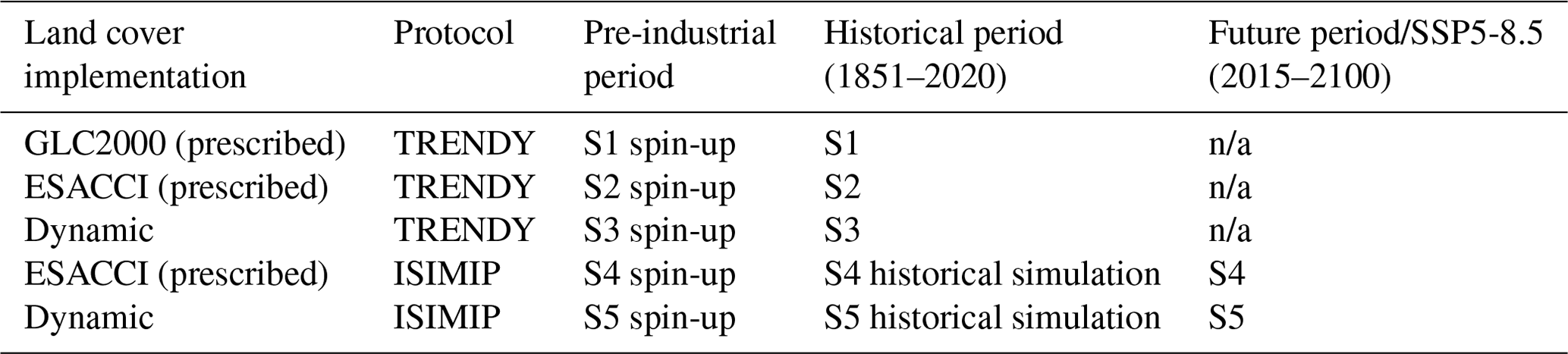
n/a: not applicable.
To evaluate dynamic land cover over the historical period (1851–2020), we conducted three simulations: two simulations with prescribed land cover (S1 and S2) and a simulation with dynamic land cover (S3). These three historical simulations were initialised from corresponding pre-industrial spin-ups (described below). Simulations with prescribed land cover use land cover forcings specifying the fractional coverage of the nine CLASSIC PFTs that are derived from two remote sensing products: the Global Land Cover 2000 (GLC2000) product (S1) (Bartholomé and Belward, 2005) and the European Space Agency Climate Change Initiative (ESACCI) version 2 product (S2) (Defourny et al., 2023). The process of generating a land cover forcing specifying the fractional coverage of all PFTs has three steps. First, the present-day fractional coverages of the model's PFTs are obtained from a remote sensing product, which involves reclassifying the land cover classes in the remote sensing product into the model's PFTs. Wang et al. (2006) describe how the 22 land cover categories in the GLC2000 product are reclassified into the nine CLASSIC PFTs. L. Wang et al. (2023) show how the 37 land cover categories in the ESACCI product from 2018 are reclassified into the nine CLASSIC PFTs. Second, the fractional coverages of crop PFTs are replaced with values from a land use change forcing for a given year in the present day, and the fractional coverages of natural PFTs are adjusted accordingly such that the total fractional coverage of vegetation is unchanged in that year. Third, the time series of fractional coverages of crop PFTs from the land use change forcing is incorporated by adjusting the fractional coverages of natural PFTs over a given time period relative to the single-year land cover forcing generated in the previous step. These three steps are used to generate a land cover forcing specifying the fractional coverage of all model PFTs derived from a remote sensing product over a given time period. Simulations with dynamic land cover use land cover forcings that only specify the fractional coverages of crop PFTs.
S1–S3 follow the TRENDY protocol (used for contributions to the Global Carbon Project) (Friedlingstein et al., 2022). The TRENDY protocol uses the merged monthly Climate Research Unit (CRU) and 6-hourly Japanese 55-year Reanalysis (JRA-55) dataset from Harris et al. (2020), atmospheric CO2 forcing from Lan et al. (2024), population density forcing from HYDE3.3 (Klein Goldewijk et al., 2017), and land use change forcing from the Land-Use Harmonization 2 (LUH2-)GCB2022 dataset (Chini et al., 2021; Hurtt et al., 2020; Klein Goldewijk et al., 2017). S1–S3 were initialised from corresponding pre-industrial spin-ups (Table 1). We conducted different pre-industrial spin-ups for each simulation that used the corresponding land cover implementation. Pre-industrial simulations used atmospheric CO2, land cover, and population density forcings corresponding to the year 1851. Pre-industrial simulations repeatedly used meteorological forcings from 1901–1920. We ran the pre-industrial spin-up until the C pools came into equilibrium. A threshold of 0.05 Pg C yr−1 for the global net atmosphere–land CO2 flux was used to assess if equilibrium was achieved. Note that all simulations exclude Antarctica and Greenland.
To examine prescribed vs. dynamic land cover over the future period (2015–2100) for SSP5-8.5 (Riahi et al., 2017), we conducted two simulations: one simulation with prescribed land cover from the ESACCI-derived land cover product (S4) and one simulation with dynamic land cover (S5). These future simulations for SSP5-8.5 were initialised from the end of their corresponding historical simulations, which were in turn initialised from their corresponding pre-industrial spin-ups (described below). S4 and S5 use bias-corrected meteorological forcings from CanESM5 (Buchner and Reyer, 2021). They use atmospheric CO2, land use change, and population density forcings from CMIP and the Inter-Sectoral Impact Model Intercomparison Project (ISIMIP) (Warszawski et al., 2014). Our study uses a single meteorological forcing (from the corresponding model CanESM5). The effects of different meteorological forcings have been explored elsewhere (Arora et al., 2023), as have the effects of bias correction (Seiler et al., 2024). S4 and S5 were initialised from the end of their corresponding historical simulations, which were in turn initialised from their corresponding pre-industrial spin-ups (Table 1). We conducted different pre-industrial spin-ups for each simulation. Pre-industrial simulations used atmospheric CO2, land use change, and population density forcings corresponding to the year 1851. Pre-industrial simulations used pre-industrial meteorological forcings provided by ISIMIP.
2.4 Model evaluation
We evaluated historical simulations using the Automated Model Benchmarking R (AMBER) package developed by Seiler et al. (2021), which quantifies model performance in reproducing observation-based datasets using a skill score system that is based on the International Land Model Benchmarking (ILAMB) framework (Collier et al., 2018). Five scores compare model output to a reference dataset for a given variable, assessing the simulated time-mean bias (Sbias), monthly centralised root mean square error (Srmse), seasonality (Sphase), interannual variability (Siav), and spatial distribution (Sdist) in comparison to the observation-based dataset. Scores are dimensionless and range from 0 to 1, where higher values indicate better model performance. The overall score for each variable (Soverall) is calculated as
For variables with more than one observation-based dataset, we calculated a benchmark score for the observation-based datasets, which quantifies how well the independently derived observation-based datasets agree with each other, thereby providing an estimate of the uncertainty in the observation-based datasets themselves. The benchmark score was calculated by iteratively comparing pairs of independently derived observation-based datasets, where one observation-based dataset is treated as model output, and the other observation dataset is treated as the reference dataset. If the two observation-based datasets were the same, the benchmark score would be 1. The calculation of each score and benchmark scores is described in detail in Seiler et al. (2022).
We adapted this statistical framework, which operates at a grid cell scale, to evaluate land cover fraction for each natural PFT within a grid cell. For simulations with dynamic land cover, we evaluated the land cover fraction for each natural PFT against both the GLC2000-derived land cover product and the ESACCI-derived land cover product. We compared the GLC2000-derived land cover product and the ESACCI-derived land cover product to obtain a benchmark score that quantifies the uncertainty in these land cover products. Note that a qualitative assessment of dynamic land cover at a spatial resolution of 2.81° in CLASSIC was presented in Melton and Arora (2016).
Additionally, we evaluated the standard set of energy, water, and C cycle variables following Seiler et al. (2022). Specifically, we evaluated aboveground biomass C (AGB), surface albedo (ALBS), area burned (BURNTAREA), soil C (CSOIL), vegetation C (CVEG), fire emissions (FIRE), gross primary productivity (GPP), soil heat flux (HFG), latent heat flux (HFLS), sensible heat flux (HFSS), leaf area index (LAI), runoff (MRRO), soil moisture (MRSLL), net biome productivity (NBP), net ecosystem exchange (NEE), ecosystem respiration (RECO), net surface longwave radiation (RLS), net surface radiation (RNS), net surface shortwave radiation (RSS), and snow water equivalent (SNW). Observation-based datasets used for evaluation are summarised in Table B2.
3.1 Historical simulations and evaluation
CLASSIC with dynamic land cover successfully reproduces the global area of trees, grasses, and total natural vegetation over the historical period, falling within the range of ESACCI- and GLC2000-derived land cover products as shown in Fig. 1. Simulated global tree, grass, and natural vegetation areas are closer to the ESACCI-derived land cover product than the GLC2000-derived land cover product for the present day (2000–2020). Over the historical period, simulated global natural vegetation area decreases due to increasing crop area, i.e., land use change (Fig. B1). Land use change is the only driver of variation in natural vegetation area in the ESACCI- and GLC2000-derived land cover products. CLASSIC with dynamic land cover simulates a smaller decrease in natural vegetation area than that attributable to land use change. This is because decreasing natural vegetation area due to land use change is partially offset by increasing natural vegetation area driven by stimulated plant growth from CO2 fertilisation and climate change over the historical period.
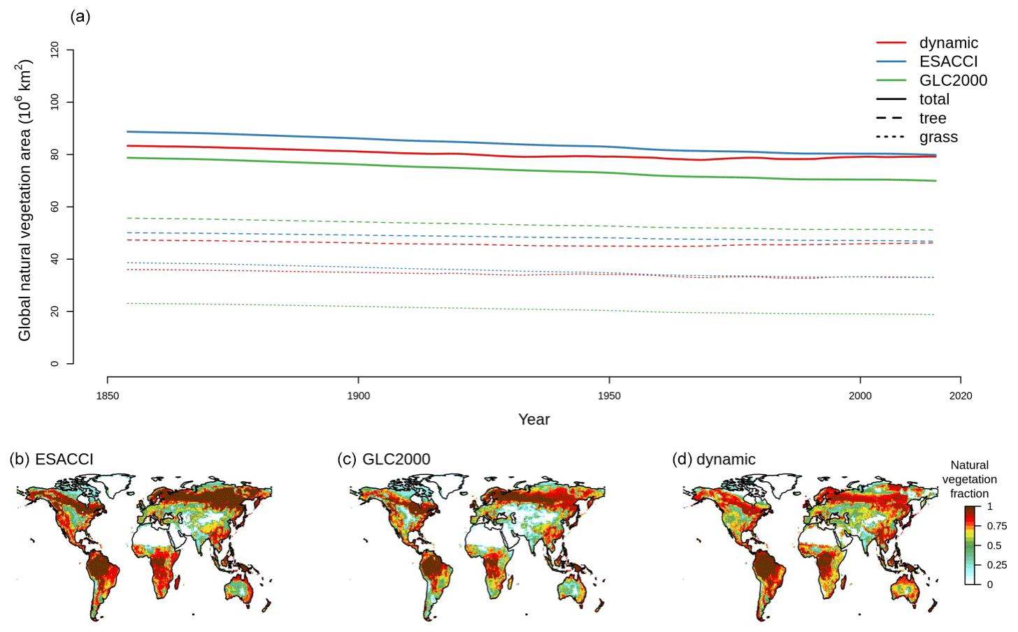
Figure 1Natural vegetation area over the historical period. (a) Global area of natural vegetation, trees, and grasses simulated by CLASSIC with dynamic land cover in comparison to ESACCI- and GLC2000-derived land cover products. Natural vegetation fraction per grid cell in the (b) ESACCI-derived land cover product and (c) GLC2000-derived land cover product and (d) simulated by CLASSIC with dynamic land cover. Simulations and land cover products are averaged over 2000–2020 in (b)–(d). Natural vegetation includes seven natural PFTs (described in Sect. 2.2), excluding crop area and bare ground.
CLASSIC with dynamic land cover also broadly reproduces the latitudinal distribution of the natural PFTs in comparison to ESACCI- and GLC2000-derived land cover products as shown in Fig. 2. However, there remain some differences between simulations and observations. CLASSIC does not simulate needleleaf evergreen trees between 20 and 40° N, whereas observations suggest that this PFT exists at these latitudes (e.g., high-elevation tropical and subtropical coniferous forests). Rather, CLASSIC simulates broadleaf deciduous cold trees at these latitudes, whereas observations suggest that this PFT declines between 40 and 20° N. Furthermore, CLASSIC slightly overestimates C4 grass area and slightly underestimates C3 grass area in the Northern Hemisphere. Reasons for these disagreements are discussed below.
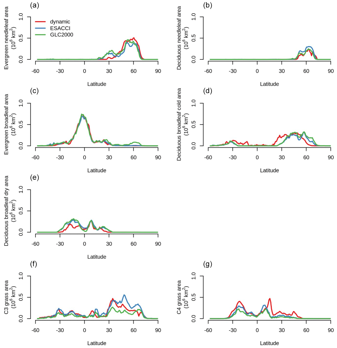
Figure 2Latitudinal distributions of each natural plant functional type (PFT) simulated by CLASSIC with dynamic land cover in comparison to ESACCI- and GLC2000-derived land cover products. (a) Evergreen needleleaf, (b) deciduous needleleaf, (c) evergreen broadleaf, (d) deciduous broadleaf cold, (e) deciduous broadleaf dry, (f) C3 grass, and (g) C4 grass. Simulations and land cover products are averaged over 2000–2020.
Both CLASSIC with prescribed land cover (simulated with ESACCI- and GLC2000-derived land cover products) and CLASSIC with dynamic land cover capture the primary C, water, and energy cycle variables (Fig. B2) reasonably well. The agreement between CLASSIC simulations and observations is quantified by scores of model performance in reproducing observation-based datasets for each biogeochemical and biophysical variable. These scores indicate that CLASSIC with dynamic land cover performed similarly to CLASSIC with prescribed land cover (Fig. B3). Figure 3a and b show model scores (averaged across all CLASSIC simulations, with both prescribed and dynamic land cover) plotted against benchmark scores for biogeochemical and biophysical variables, respectively. Figure 3 shows the correspondence between model performance in reproducing observation-based datasets (i.e., model scores) and the uncertainty in the observation-based datasets themselves (i.e., benchmark scores). Model scores for both versions of CLASSIC (prescribed and dynamic land cover) and benchmark scores are similar, falling close to the 1:1 line, which indicates that model performance is comparable to the uncertainty in the observation-based datasets themselves. Both versions of CLASSIC perform slightly better for biophysical variables (Fig. 3b) than for biogeochemical variables (Fig. 3a). Finally, CLASSIC with both prescribed and dynamic land cover simulates the terrestrial C sink over the historical period reasonably well in comparison to other models in the Global Carbon Project (Friedlingstein et al., 2022) (Fig. B4).
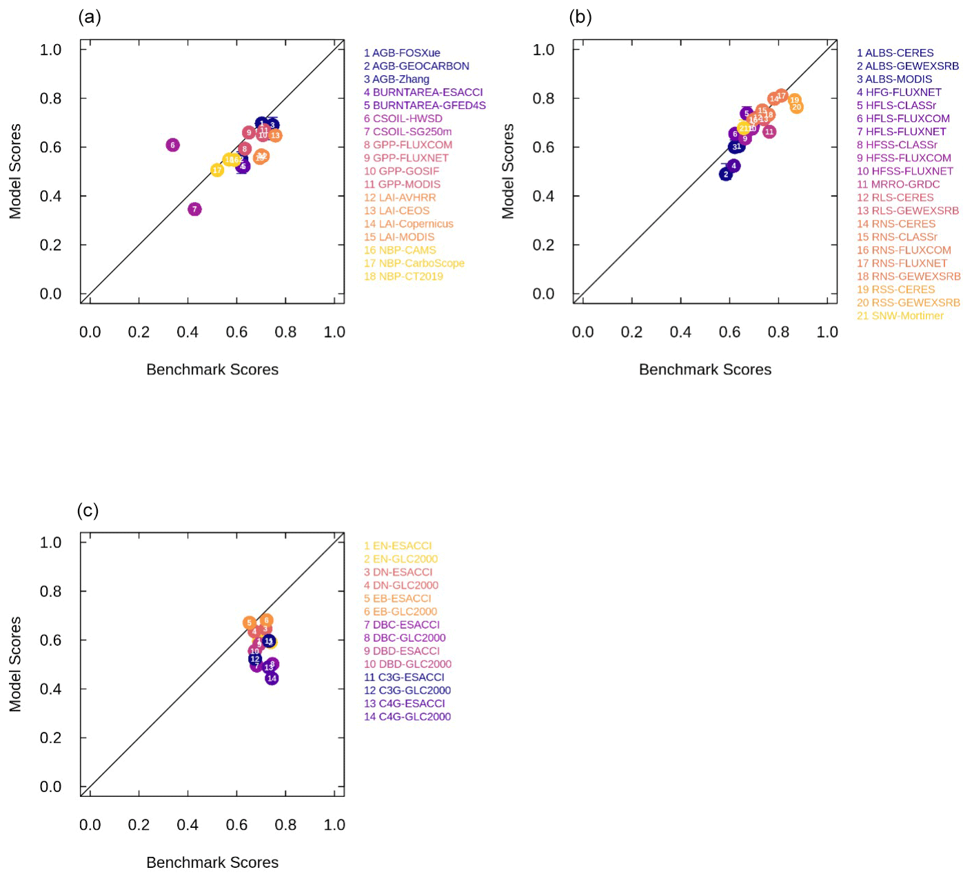
Figure 3Model performance in reproducing observation-based datasets (model scores) relative to the uncertainty in the observation-based datasets themselves (benchmark scores) for (a) biogeochemical variables, (b) biophysical variables, and (c) land cover fractions of each natural plant functional type (PFT). Model scores are averaged across simulations of CLASSIC with prescribed land cover (with an ESACCI-derived land cover forcing and a GLC2000-derived land cover forcing) and dynamic land cover for biogeochemical and biophysical variables. Whiskers indicate the maximum and minimum model scores. Abbreviations for C, water, and energy variables and observation-based datasets are described in the Methods section. Abbreviations for PFTs are evergreen needleleaf (EN), deciduous needleleaf (DN), evergreen broadleaf (EB), deciduous broadleaf cold (DBC), deciduous broadleaf dry (DBD), C3 grass (C3G), and C4 grass (C4G).
When dynamic land cover is implemented in CLASSIC, the ability of CLASSIC to reproduce land cover fractions of each natural PFT can be assessed alongside C, water, and energy variables as shown in Fig. 3c. Additionally, benchmark scores can be calculated for the land cover fractions of each natural PFT by comparing the ESACCI-derived land cover product to the GLC2000-derived land cover product. Model scores tend to be lower than benchmark scores, especially for tropical PFTs (broadleaf deciduous dry trees and C4 grasses). For these PFTs uncertainty is introduced because remote sensing products do not distinguish between cold and dry broadleaf deciduous trees and between C3 and C4 grasses. This distinction is made during the reclassification of the land cover categories into the nine CLASSIC PFTs and introduces some subjectivity (L. Wang et al., 2023). Specifically, deciduous trees above 30° in both hemispheres are assumed to be cold deciduous, deciduous trees below 20° in both hemispheres are assumed to be dry deciduous, and the fraction of trees that are cold vs. dry deciduous varies linearly between 0 and 1 with latitude for deciduous trees between 20 and 30°. The separation of grasses into C3 and C4 is based on the time-invariant global product from Still et al. (2003).
3.2 Future simulations
For SSP5-8.5, CLASSIC with dynamic land cover simulates the increasing global area of trees, grasses, and total natural vegetation (Fig. 4a). Global natural vegetation area decreases in the ESACCI-derived land cover product due to land use change (increasing crop area), which is again the only driver of variation in natural vegetation area in the ESACCI-derived land cover product (Figs. 4a, B1). Decreasing natural vegetation area due to land use change occurs primarily in South America, Africa, and Asia (Fig. 4b). CLASSIC with dynamic land cover simulates increasing natural vegetation area because the loss of natural vegetation area due to land use change is offset by increasing natural vegetation area, especially at high latitudes (Fig. 4c).
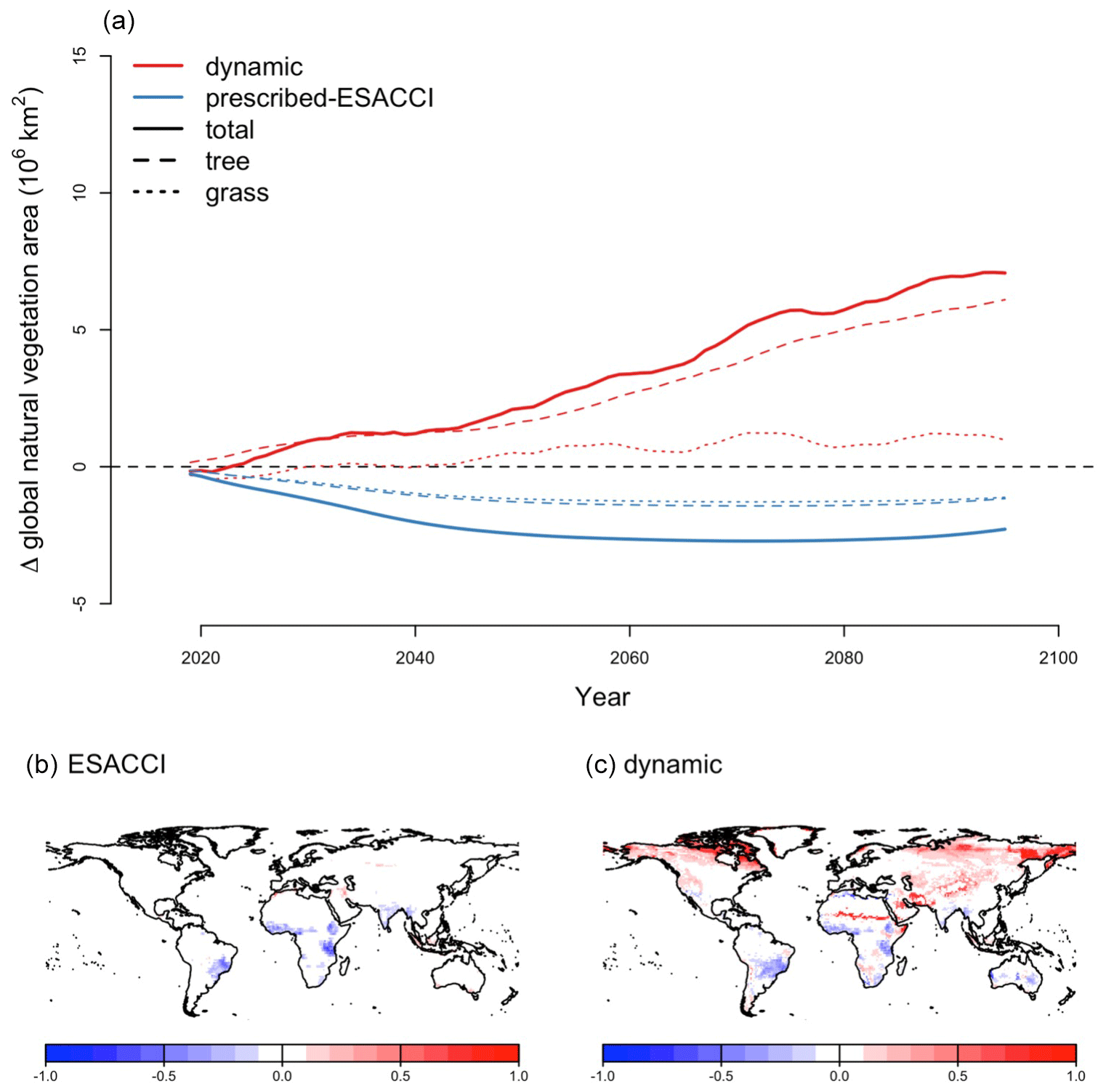
Figure 4Change in natural vegetation area for SSP5-8.5 (2015–2100). (a) Change in global area of natural vegetation, trees, and grasses simulated by CLASSIC with dynamic land cover in comparison to the ESACCI-derived land cover product. Change in natural vegetation fraction per grid cell (b) in the ESACCI-derived land cover product and (c) simulated by CLASSIC with dynamic land cover. Differences reflect the change between the averages calculated over 1995–2015 and 2080–2100. Only grid cells with a significant temporal trend are shown (P<0.05; assessed with a Mann–Kendall trend test). Figure B5 shows the change in fraction per grid cell for each PFT simulated by CLASSIC with dynamic land cover. Figure B13 shows the absolute value of the natural vegetation fraction per grid cell averaged over 1995–2015 and 2080–2100 simulated by CLASSIC with prescribed land cover and CLASSIC with dynamic land cover.
At high latitudes, CLASSIC with dynamic land cover simulates increasing areas of needleleaf evergreen trees, broadleaf deciduous cold trees, and C3 and C4 grasses, expanding into what was previously bare ground (Fig. B5). This corresponds to increasing temperatures at high latitudes (Fig. B6). In particular, C4 grasses, which are currently primarily found at low latitudes, expand into high latitudes due to their dependence on temperature (Luo et al., 2024). At low latitudes, CLASSIC with dynamic land cover simulates decreasing natural vegetation area in South America but variably decreasing and increasing natural vegetation area in Africa and Asia. In the Amazon, the area of broadleaf evergreen trees decreases, while the areas of C3 and C4 grasses increase (Fig. B5). This corresponds to decreasing precipitation in this region (Fig. B6). Conversely, in Africa and Asia, the area of broadleaf evergreen trees increases, while the areas of C3 and C4 grasses decrease (Fig. B5). This corresponds to increasing precipitation in this region (Fig. B6). As an exception, in the Sahel, the areas of C3 and C4 grasses increase, expanding into what was previously bare ground (Fig. B5). This also corresponds to increasing precipitation in this region (Fig. B6).
CLASSIC with prescribed land cover (simulated with an ESACCI-derived land cover product) and CLASSIC with dynamic land cover both simulate increasing net primary productivity (NPP) at higher latitudes for SSP5-8.5 (Fig. 5a–b). NPP increases to a greater extent at higher latitudes in the simulation with dynamic land cover because of increasing natural vegetation area, especially that of broadleaf trees at the expense of needleleaf trees (Figs. 5c–f and 6a–c). NPP changes are similar at lower latitudes in both versions of CLASSIC (Fig. 5a–b). Both versions of CLASSIC project decreasing NPP in the Amazon (Fig. 5a–b). NPP decreases in simulations with prescribed land cover due to decreasing precipitation in the Amazon (Fig. B6). NPP decreases slightly less in the simulation with dynamic land cover because decreasing tree area and NPP are offset by increasing grass area and NPP in the Amazon (Figs. 5c–f and 6d–f). In the Sahel, NPP increases slightly in the simulation with dynamic land cover but decreases slightly in the simulation with prescribed land cover (Fig. 5a–b). NPP decreases in simulations with prescribed land cover due to land use change in the Sahel (Fig. 6h). NPP increases slightly in the simulation with dynamic land cover because of increasing grass area, outweighing the effects of NPP in the Sahel (Figs. 5c–f and 6g–i). Both versions of CLASSIC simulate similar increases in vegetation C (Figs. B7 and B8). CLASSIC with dynamic land cover simulates a smaller decrease in soil C due to increased natural vegetation area at high latitudes (Figs. B7 and B9).
CLASSIC dynamically simulates fire (Arora and Melton, 2018). When prescribed land cover is implemented, fire reduces vegetation biomass density, whereas when dynamic land cover is implemented, fire both reduces vegetation biomass density and creates bare ground that can then be colonised by a different plant functional type. CLASSIC with dynamic land cover simulates slightly higher area burned and fire CO2 emissions than CLASSIC with prescribed land cover at the global scale due to higher natural vegetation area (Fig. B10), but spatial patterns are relatively similar between both versions of CLASSIC (Figs. B11 and B12). In particular, neither version of CLASSIC simulates substantial changes in high-latitude fires, which CLASSIC underestimates (Arora and Melton, 2018). CLASSIC with dynamic land cover simulates lower fire in the Amazon and higher fire in the Sahel, corresponding to lower and higher natural vegetation area in the Amazon and Sahel, respectively. This suggests that there are minor differences in fire occurrence between different PFTs, which should be improved in future model development.
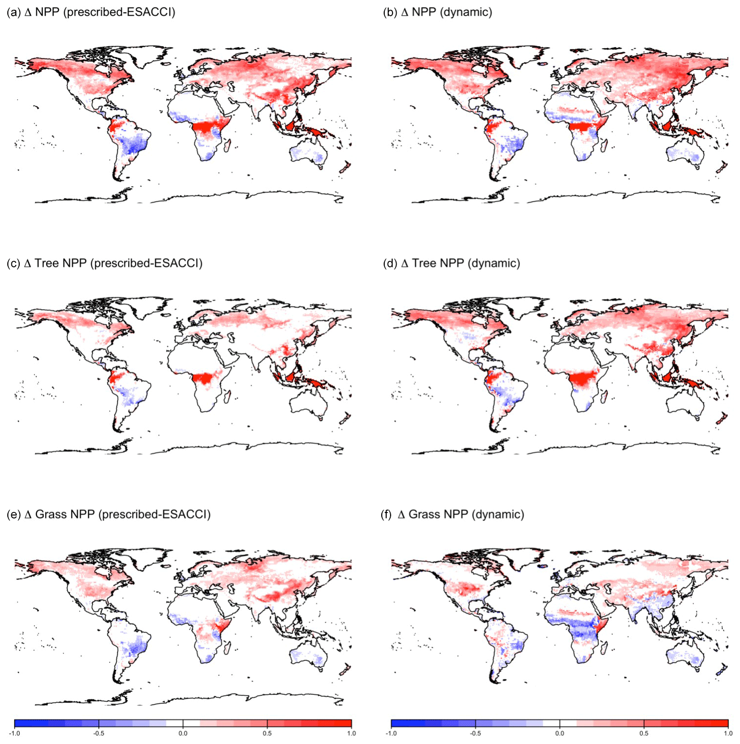
Figure 5Change in net primary productivity (NPP) simulated by CLASSIC with prescribed land cover (with an ESACCI-derived land cover forcing) and CLASSIC with dynamic land cover for SSP5-8.5 (2015–2100). (a, b) Total NPP, (c, d) tree NPP, and (e, f) grass NPP. Differences reflect the change between the average over 1995–2015 and 2080–2100. Only grid cells with a significant temporal trend are shown (P<0.05; assessed with a Mann–Kendall trend test).
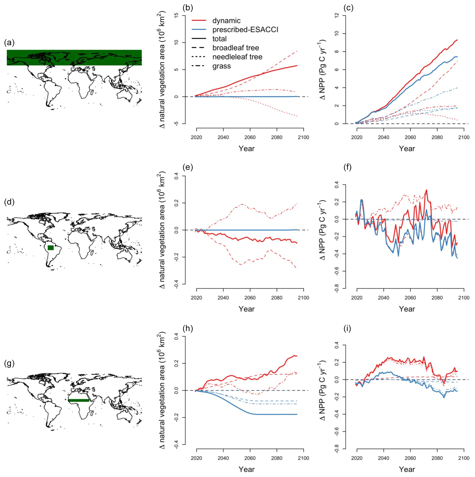
Figure 6Change in natural vegetation area and net primary productivity (NPP) at high latitudes, the Amazon, and the Sahel by CLASSIC with prescribed land cover (with an ESACCI-derived land cover forcing) and CLASSIC with dynamic land cover for SSP5-8.5 (2015–2100). (a) Map of high latitudes. (b) Change in global area of natural vegetation, broadleaf trees, needleleaf trees, and grasses in high latitudes. (c) Change in NPP in high latitudes. (d) Map of the Amazon. (e) Change in global area of natural vegetation, broadleaf trees, needleleaf trees, and grasses in the Amazon. (f) Change in NPP in the Amazon. (g) Map of the Sahel. (h) Change in global area of natural vegetation, broadleaf trees, needleleaf trees, and grasses in the Sahel. (i) Change in NPP in the Sahel.
Net biome productivity (NBP), i.e., the net land–atmosphere CO2 flux (which includes photosynthesis, autotrophic and heterotrophic respiration, fire emissions, and land use change emissions), increases in CLASSIC simulations of SSP5-8.5 with both prescribed and dynamic land cover (Fig. 7a). The increase in NBP is almost 2-fold greater in the simulation with dynamic land cover (5.28 Pg C yr−1 averaged over 2080–2100) than in the simulation with prescribed land cover (2.29 Pg C yr−1 averaged over 2080–2100). At the global scale, this increase in NBP is driven by increasing NPP (Fig. 7b–c), which is primarily due to CO2 fertilisation in both versions of CLASSIC. In CLASSIC with dynamic land cover, there is a stronger NPP increase at high northern latitudes (Fig. 7c). NPP increases at low latitudes in both versions of CLASSIC because increasing NPP in Africa and Asia outweighs decreasing NPP in South America. The change in NPP at low latitudes is similar between both versions of CLASSIC despite changing tree vs. grass areas as described above due to offsetting effects. Surface albedo decreases due to snow loss driven by increasing temperature in both versions of CLASSIC (Fig. 7d), but this decrease is slightly stronger at high northern latitudes in CLASSIC with dynamic land cover due to the expansion of natural vegetation into higher latitudes (Fig. 7e). Evapotranspiration increases in both versions of CLASSIC (Fig. 7f), but this increase is slightly stronger at high northern latitudes in CLASSIC with dynamic land cover due to the expansion of natural vegetation into higher latitudes (Fig. 7g).
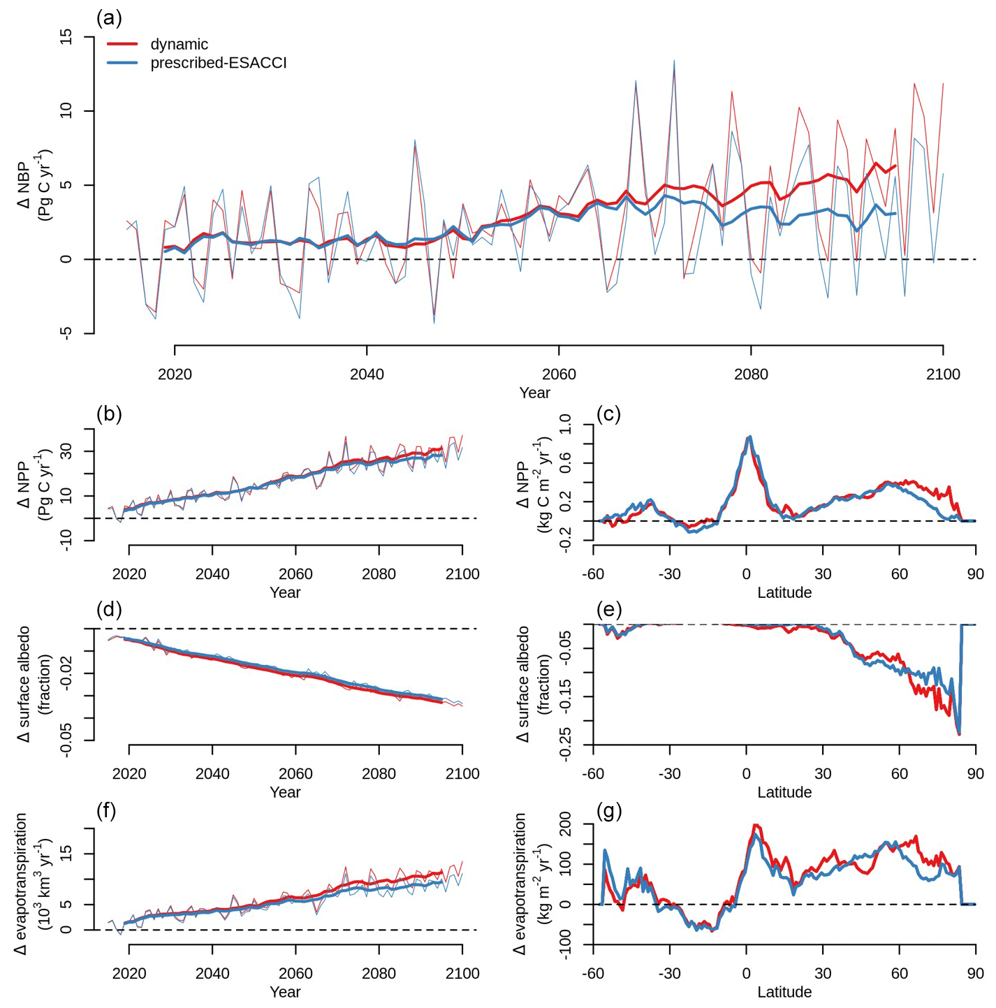
Figure 7Change in (a) net biome productivity (NBP), (b, c) net primary productivity (NPP), (d, e) surface albedo, and (f, g) evapotranspiration simulated by CLASSIC with prescribed land cover (with an ESACCI-derived land cover forcing) and CLASSIC with dynamic land cover for SSP5-8.5 (2015–2100). For the latitudinal distributions, CLASSIC simulations were averaged over 2080–2100. Thin lines indicate the annual value, and thick lines indicate the moving average over 10 years.
Dynamic land cover is rarely implemented in terrestrial biosphere models (e.g., in only 3 out of 11 models contributing to C4MIP within the sixth phase of CMIP), and the simulated geographical distribution of natural vegetation has not yet been evaluated robustly as it lacked the methodology to do so. The Global Carbon Project uses a statistical framework to evaluate the ability of its models to reproduce observations of the C, water, and energy cycles – the International Land Model Benchmarking (ILAMB) framework (Collier et al., 2018) – which has since been expanded to include a method to quantify the uncertainty in the observation-based datasets themselves (Seiler et al., 2022). We build on this to introduce a framework with which the dynamically simulated geographical distribution of natural vegetation can be quantitatively evaluated against observations. We use this framework to show that CLASSIC with dynamic land cover successfully simulates the geographical distribution of its natural PFTs for the present day, reproducing observations (Figs. 1–3). This framework can be applied across terrestrial biosphere models to evaluate dynamic land cover alongside evaluations of the principal C, water, and energy cycle processes.
Future projections for Shared Socioeconomic Pathway 5-8.5 (fossil-fuelled development scenario, SSP5-8.5) differ significantly between simulations with prescribed and dynamic land cover because in the latter the geographical distribution of natural vegetation is able to respond to changing environmental conditions. The net land–atmosphere CO2 flux (or net biome productivity, NBP) is nearly twice as large in the simulation with dynamic land cover (5.28 Pg C yr−1 averaged over 2080–2100) than in the simulation with prescribed land cover (2.29 Pg C yr−1 averaged over 2080–2100) (Fig. 7). This difference is attributed to three important range shifts that are only simulated when dynamic land cover is implemented: (1) the expansion of trees into high latitudes, which increases NBP; (2) the recession of trees accompanied by the expansion of grasses in the Amazon, which decreases NBP; and (3) the expansion of grasses into the Sahel, which increases NBP (Figs. 5, 6, and 7). These responses occurred over the historical period as well but to a much smaller extent (Fig. 1). We now discuss each of these range shifts in greater detail.
“Greening of the Arctic” describes the expansion of vegetation into high-latitude regions, which occurs as previously uninhabitable regions become habitable due to increasing temperatures (Chen et al., 2011; Elmendorf et al., 2012; Myers-Smith et al., 2020; Pearson et al., 2013; Piao et al., 2020; Tape et al., 2006). While terrestrial biosphere models with prescribed land cover capture increasing plant growth at high latitudes within their present-day range due to increasing temperatures (J. Wang et al., 2023), these models are not able to simulate range shifts. Our results suggest these range shifts could make a sizeable contribution to the terrestrial C sink via C sequestration in vegetation and soils at high latitudes due to the northward expansion of trees and grasses. Fire alongside rising temperature is known to drive a transition from needleleaf trees to broadleaf trees (Hisano et al., 2021). Because broadleaf trees are less flammable than needleleaf trees, this transition could reduce fire activity (Baltzer et al., 2021; Johnstone and Chapin, 2006; Mack et al., 2021). These processes are not represented explicitly here but warrant further study, especially given their importance and significant biases across land surface models at high latitudes (Braghiere et al., 2023; Wang et al., 2021). Although the greening of the Arctic drives increased terrestrial C sequestration at high latitudes, it also drives other important feedbacks to the climate system, such as reduced albedo (Chapin et al., 2005) and enhanced evapotranspiration (Swann et al., 2010).
“Amazonian dieback” describes the combination of deforestation and the increased mortality of trees in the Amazon rainforest due to changing climate in the region (Malhi et al., 2008; Parry et al., 2022). Tree mortality occurs as previously habitable regions become inhabitable due to the sensitivity of trees to drought and heat stress (Aleixo et al., 2019; Phillips et al., 2009). While the direct effects of reduced precipitation and elevated temperature on plant growth as well as deforestation are captured by terrestrial biosphere models with prescribed land cover, these models are incapable of simulating transitions from forest to grassland. Fire modulates these transitions, as grasses rapidly regenerate post-fire and are more flammable than trees, thereby intensifying fire activity (Davidson et al., 2012). Finally, Amazonian dieback self-amplifies via feedbacks to the climate system, as decreased forest cover decreases evapotranspiration, which could amplify regional drought (Zemp et al., 2017). The effects of these feedbacks and the feedbacks associated with the greening of the Arctic are not evaluated in our offline simulations and warrant further study.
Finally, the “greening of the Sahel” describes the expansion of vegetation into the Sahara, which occurs as previously uninhabitable regions become habitable due to increasing precipitation (Brandt et al., 2015; Herrmann et al., 2005; Olsson et al., 2005). This range shift is not captured in terrestrial biosphere models with prescribed land cover. However, there is large uncertainty in future projections of precipitation in this region (Monerie et al., 2020). While less explored than the previous two effects, greening of the Sahel is regionally important and could make a non-trivial contribution to the global C, water, and energy cycles, warranting further study.
These responses are consistent with those of other terrestrial biosphere models that implement dynamic land cover. Both Scholze et al. (2006) and Alo and Wang (2008) simulated increasing tree area at high latitudes and the replacement of trees with grasses in the Amazon. Sitch et al. (2008), who compared four models with dynamic land cover, found similar results, although the magnitudes of the responses differed between models. Port et al. (2012) conducted and examined a fully coupled simulation with a land model with dynamic land cover and similarly observed both greening of the Arctic and Amazonian dieback. Because there is large uncertainty in climate projections in the Sahel region, greening of the Sahel is often but not always simulated (Sitch et al., 2008). Our results follow the consistent pattern simulated by these other models, but our unique experimental design allows us to isolate the impact of dynamic land cover implementation (vs. prescribed land cover implementation) and compare it against the effects of other global change drivers.
Our results illustrate the potential effects of range shifts alongside variation in plant growth that is driven by climate change. While all terrestrial biosphere models account for the influence of global change drivers such as CO2 fertilisation, increasing temperatures, and variable precipitation regimes on plant growth, terrestrial biosphere models with prescribed land cover cannot capture range shifts that are driven by climate change. However, few terrestrial biosphere models incorporate dynamic land cover. Importantly, the shifting ranges of biomes have critical feedbacks to climate change and critical consequences for biodiversity and human well-being (Pecl et al., 2017) alongside their consequences for the global C cycle.
When dynamic land cover is implemented, the fractional coverage of a natural PFT is the result of colonisation and mortality (described in detail in Melton and Arora, 2016). The colonisation rate of PFT n (cn; d−1) is determined by its net primary productivity (NPP):
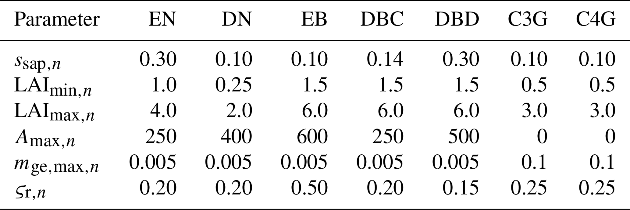
where NPPn is the NPP of PFT n, and Cveg,n is the vegetation C biomass of PFT n. ssap,n is a factor for converting vegetation C biomass to seedling C biomass of PFT n (unitless) (Table B3). λ1,n and λ2,n determine the fraction of NPP that is used for spatial expansion within a given grid cell of PFT n (unitless):
LAImin,n and LAImax,n are the minimum and maximum leaf area index thresholds of PFT n (m2 m−2), respectively (Table B3).
The mortality rate of PFT n (mn; d−1) is the sum of intrinsic or age-related mortality (mintr,n; d−1), mortality due to reduced growth (mge,n; d−1), mortality due to fire (mdist,n; d−1), and mortality when a PFT exists outside its bioclimatic limits (mbioclim,n; d−1):
where Amax,n is the maximum age of PFT n (year) (Table B3), and is the maximum growth-related mortality rate occurring when no growth occurs in PFT n (d−1) (Table B3). gen is the growth efficiency over the previous year of PFT n (kg C m−2):
where ΔCs,n is the stem C increment over the previous year of PFT n (kg C m−2), ΔCr,n is the root C increment over the previous year of PFT n (kg C m−2), and Lmax,n is the maximum LAI over the previous year of PFT n (m2 m−2). ςr,n is the susceptibility to stand-replacing fire of PFT n (fraction) (Table B3). fburned,n is the fractional area burned within a day of PFT n and depends on wind speed, soil moisture, and the probability of fire occurrence (which depends on the availability of vegetation biomass as a fuel source, the combustibility of the fuel source based on soil moisture, and the presence of an ignition source based on lightning and population density) and suppression (which depends on population density). This is described in detail in Arora and Melton (2018).
Six bioclimatic indices are used to determine the spatial range of PFTs, representing the physiological limits to their survival: air temperature of the coldest month, air temperature of the warmest month, aridity index (ratio of potential evaporation to precipitation), growing degree days (cumulative number of days with air temperature above 5 °C), dry-season length (number of consecutive months with precipitation less than potential evaporation), and precipitation surplus (difference between precipitation and potential evaporation). Bioclimatic indices for each grid cell are updated annually on a 25-year timescale using exponential smoothing:
where x(t) represents a bioclimatic index at year t, and X(t) represents the smoothed bioclimatic index at year t. This accounts for time lags in the response of vegetation to climate change drivers (Wu et al., 2015). At the beginning of each time step, each grid cell is assigned with a small fractional coverage of each PFT (0.001). Whether the PFT persists is determined by when any bioclimatic index is outside its corresponding bioclimatic limit for a given PFT, and when all bioclimatic indices are inside their corresponding bioclimatic limits for a given PFT. Bioclimatic limits for each PFT are given in Table B1. These were derived by first calculating the bioclimatic indices for each grid cell using the CRUJRA climate dataset averaged over 1900–1920 (Harris et al., 2020). Then, the 1 % and 99 % quantiles of these bioclimatic indices over all grid cells for each land cover type in the Collection 5 MODIS Global Land Cover Type International Geosphere-Biosphere Programme (IGBP) product (Friedl et al., 2010) were calculated and associated with a CLASSIC PFT. Note that this assumes that the current biome ranges are in equilibrium with the 1900–1920 climate.
Each natural PFT is given a dominance rank (i), where PFTs with higher dominance ranks invade PFTs with lower dominance ranks and bare ground. Natural PFTs cannot invade crop area. Tree PFTs are given higher dominance ranks than grass PFTs. Within tree PFTs and within grass PFTs, a PFT with a higher cn is dominant over all PFTs with lower cn. Each PFT is thus ranked from , where the PFT with dominance rank 1 is the most dominant. Overall, the change in fractional coverage of a PFT with dominance rank i is due to (1) its colonisation into the areas of PFTs with lower dominance ranks ( and bare ground (N+1), (2) colonisation by PFTs with higher dominance ranks () into its area, and (3) its mortality:
The change in fractional coverage of bare ground is due to mortality of the PFTs and colonisation of bare ground by the PFTs:
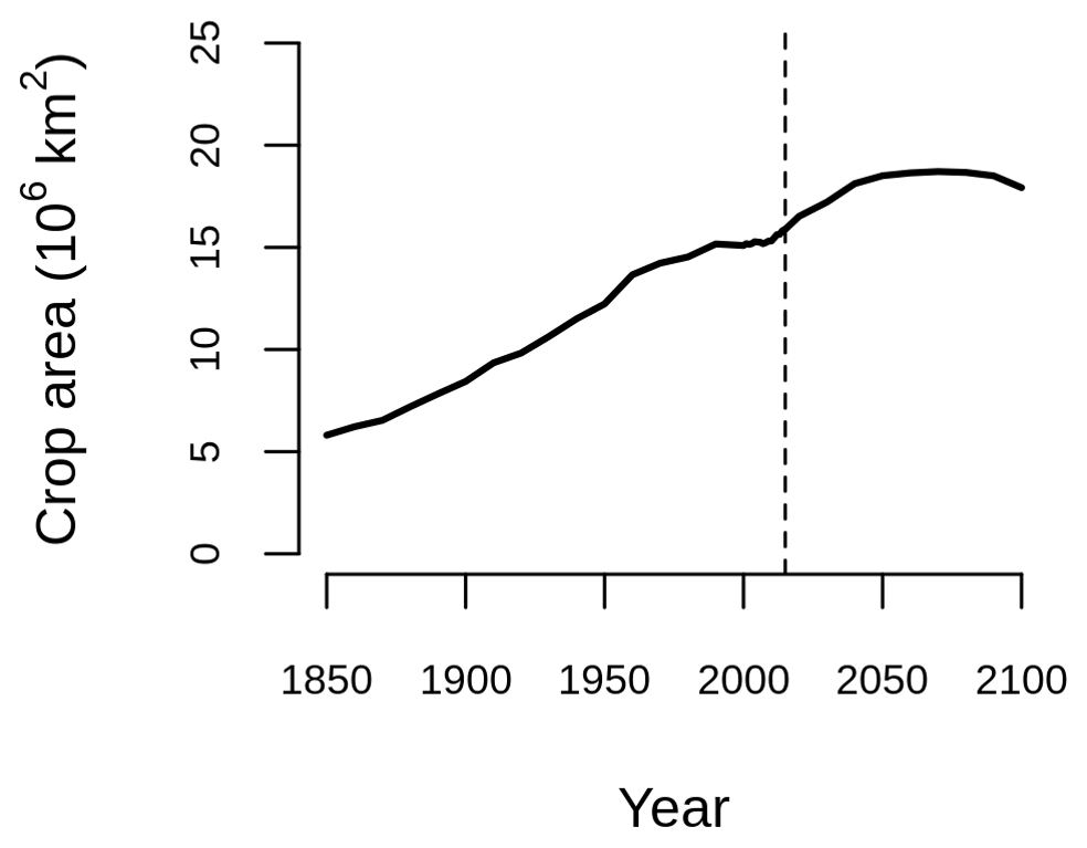
Figure B1Crop area over the historical period (1850–2015) and SSP5-8.5 (2015–2100) from the Land-Use Harmonization 2 (LUH2-)GCB2022 dataset (Chini et al., 2021; Hurtt et al., 2020; Klein Goldewijk et al., 2017).
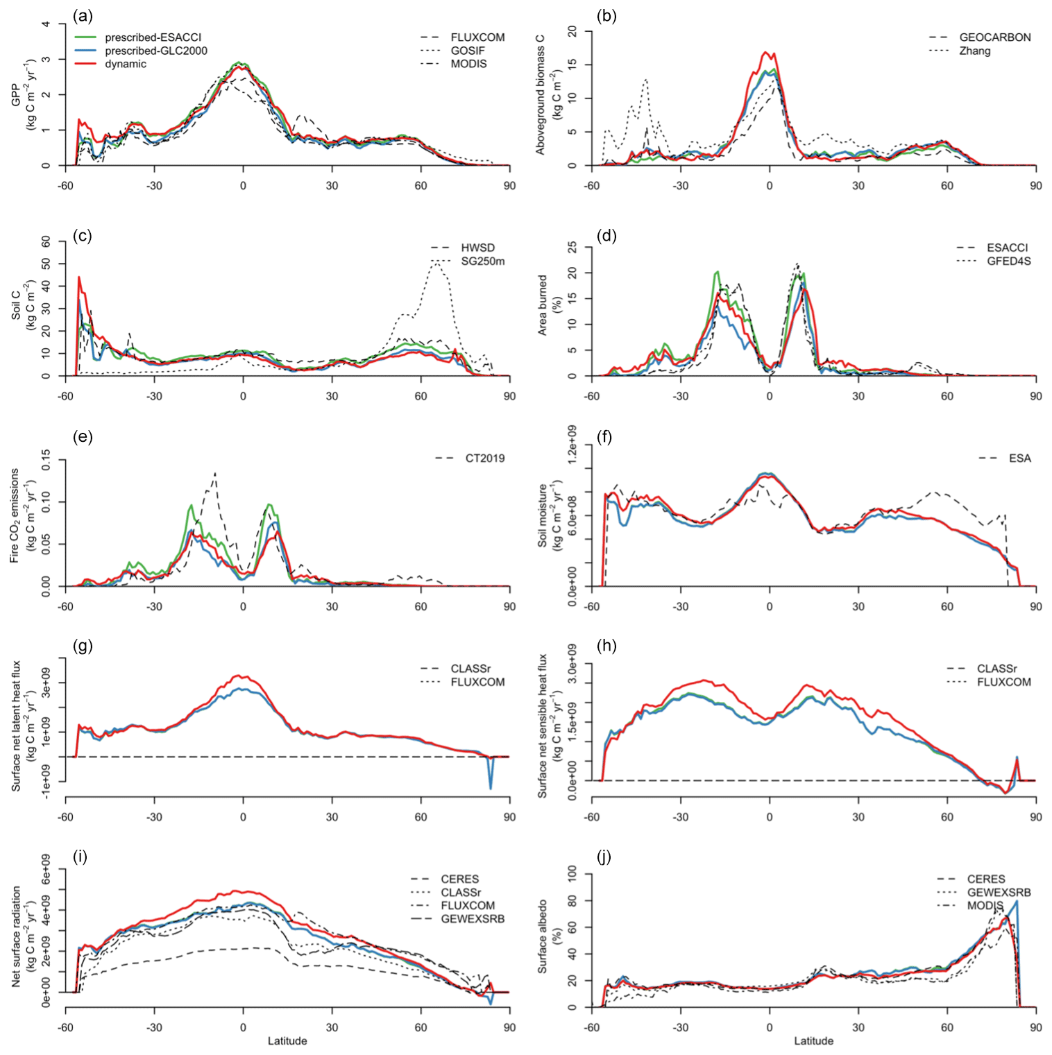
Figure B2Latitudinal distributions of (a) gross primary productivity (GPP), (b) aboveground biomass C, (c) soil C, (d) area burned, (e) fire CO2 emissions, (f) soil moisture, (g) surface net latent heat flux, (h) surface net sensible heat flux, (i) net surface radiation, and (j) surface albedo simulated by CLASSIC with prescribed land cover (with an ESACCI-derived land cover forcing and a GLC2000-derived land cover forcing) and CLASSIC with dynamic land cover in comparison to present-day observations. CLASSIC simulations were averaged over 2000–2020. Observation-based datasets are described in the Methods section. Figure B2 shows the scores of model performance in reproducing observation-based datasets for each variable.
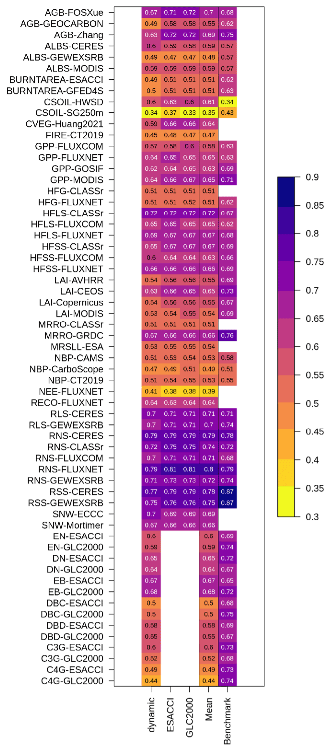
Figure B3Scores of model performance in reproducing observation-based datasets of principal C, water, and energy variables as well as land cover fractions of each natural plant functional type (PFT) for simulations of CLASSIC with prescribed land cover (with an ESACCI-derived land cover forcing and a GLC2000-derived land cover forcing) and dynamic land cover. Abbreviations for C, water, and energy variables and observation-based datasets are described in the Methods section. Abbreviations for PFTs are evergreen needleleaf (EN), deciduous needleleaf (DN), evergreen broadleaf (EB), deciduous broadleaf cold (DBC), deciduous broadleaf dry (DBD), C3 grass (C3G), and C4 grass (C4G).
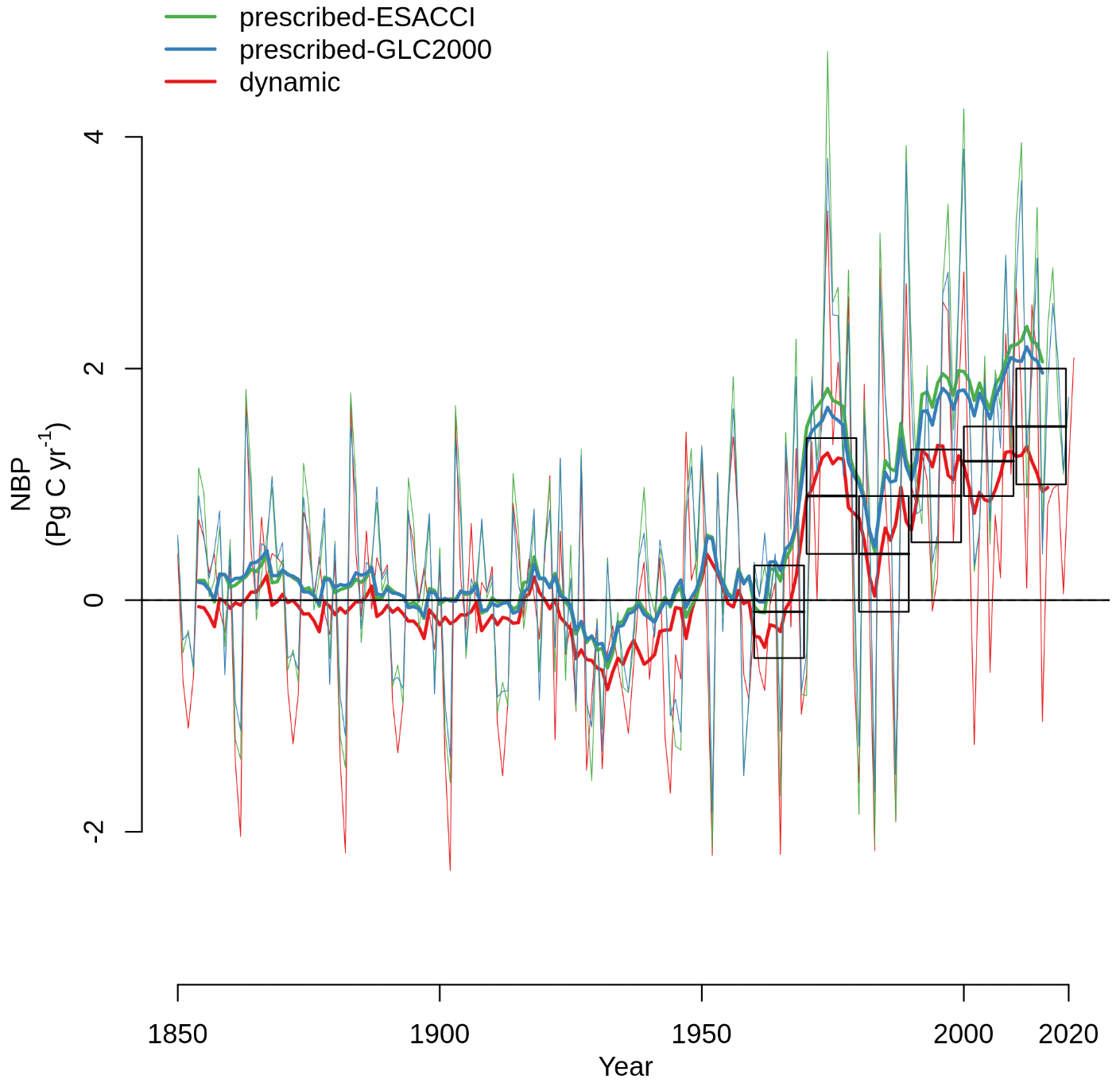
Figure B4Net biome productivity (NBP) simulated by CLASSIC with prescribed land cover (with an ESACCI-derived land cover forcing and a GLC2000-derived land cover forcing) and CLASSIC with dynamic land cover. Boxes indicate estimates from the suite of models in the Global Carbon Project, where dark horizontal lines indicate the mean, and the extent indicates 1 standard deviation (Friedlingstein et al., 2022). Thin lines indicate the annual value, and thick lines indicate the moving average over 10 years.
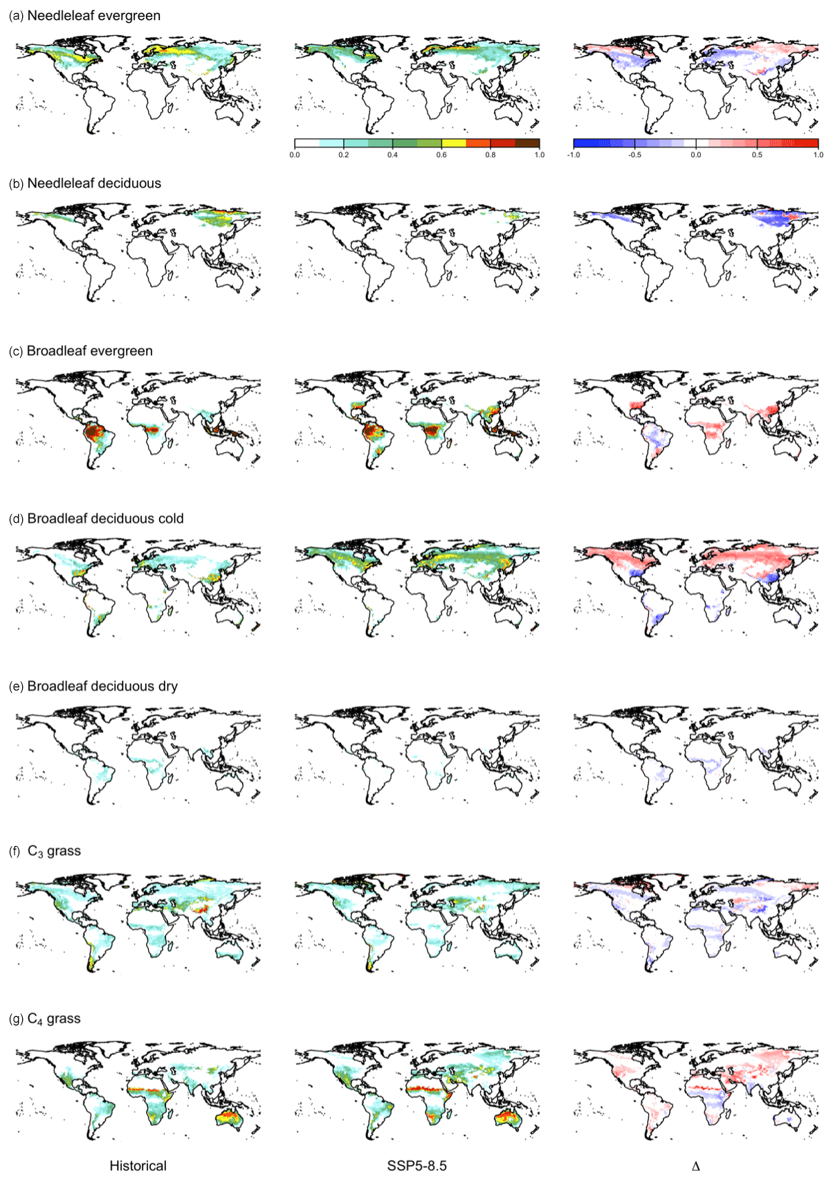
Figure B5Fraction per grid cell in the historical period (averaged over 1995–2015), in SSP5-8.5 (averaged over 2080–2100), and change between the historical period and SSP5-8.5 for each plant functional type (PFT) simulated by CLASSIC with dynamic land cover. (a) Evergreen needleleaf, (b) deciduous needleleaf, (c) evergreen broadleaf, (d) deciduous broadleaf cold, (e) deciduous broadleaf dry, (f) C3 grass, and (g) C4 grass. Differences reflect the change between the average over 1995–2015 and 2080–2100.
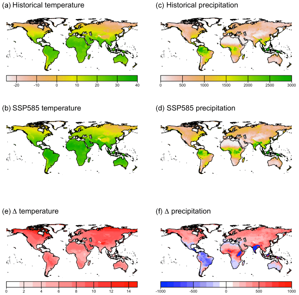
Figure B6Temperature and precipitation in (a, c) the historical period (averaged over 1995–2015) and (b, d) SSP5-8.5 (averaged over 2080–2100) and (e, f) temperature and precipitation difference between the historical period and SSP5-8.5.
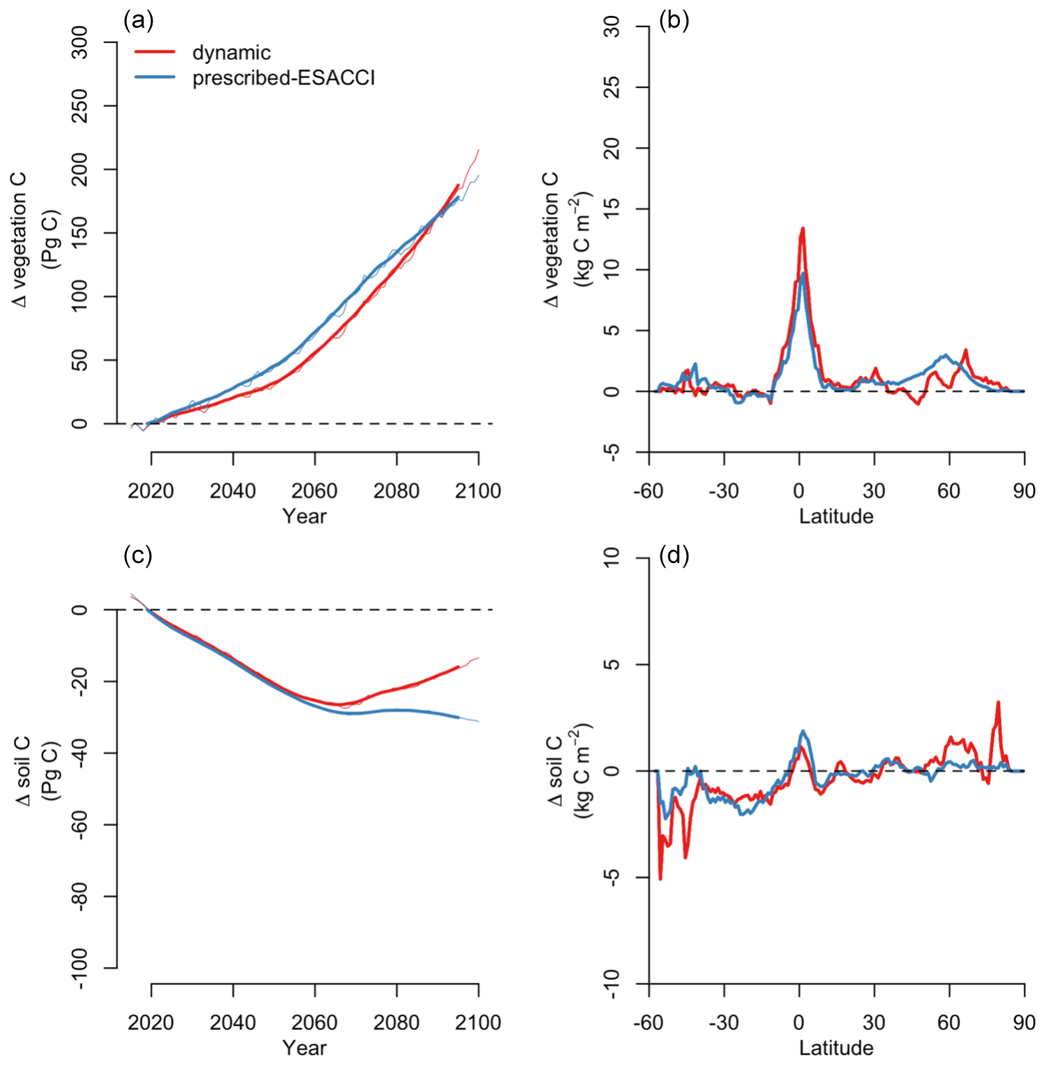
Figure B7(a, b) Change in vegetation C and (c, d) soil C simulated by CLASSIC with prescribed land cover (with an ESACCI-derived land cover forcing) and CLASSIC with dynamic land cover for SSP5-8.5 (2015–2100). For the latitudinal distributions, CLASSIC simulations were averaged over 2080–2100. Thin lines indicate the annual value, and thick lines indicate the moving average over 10 years.
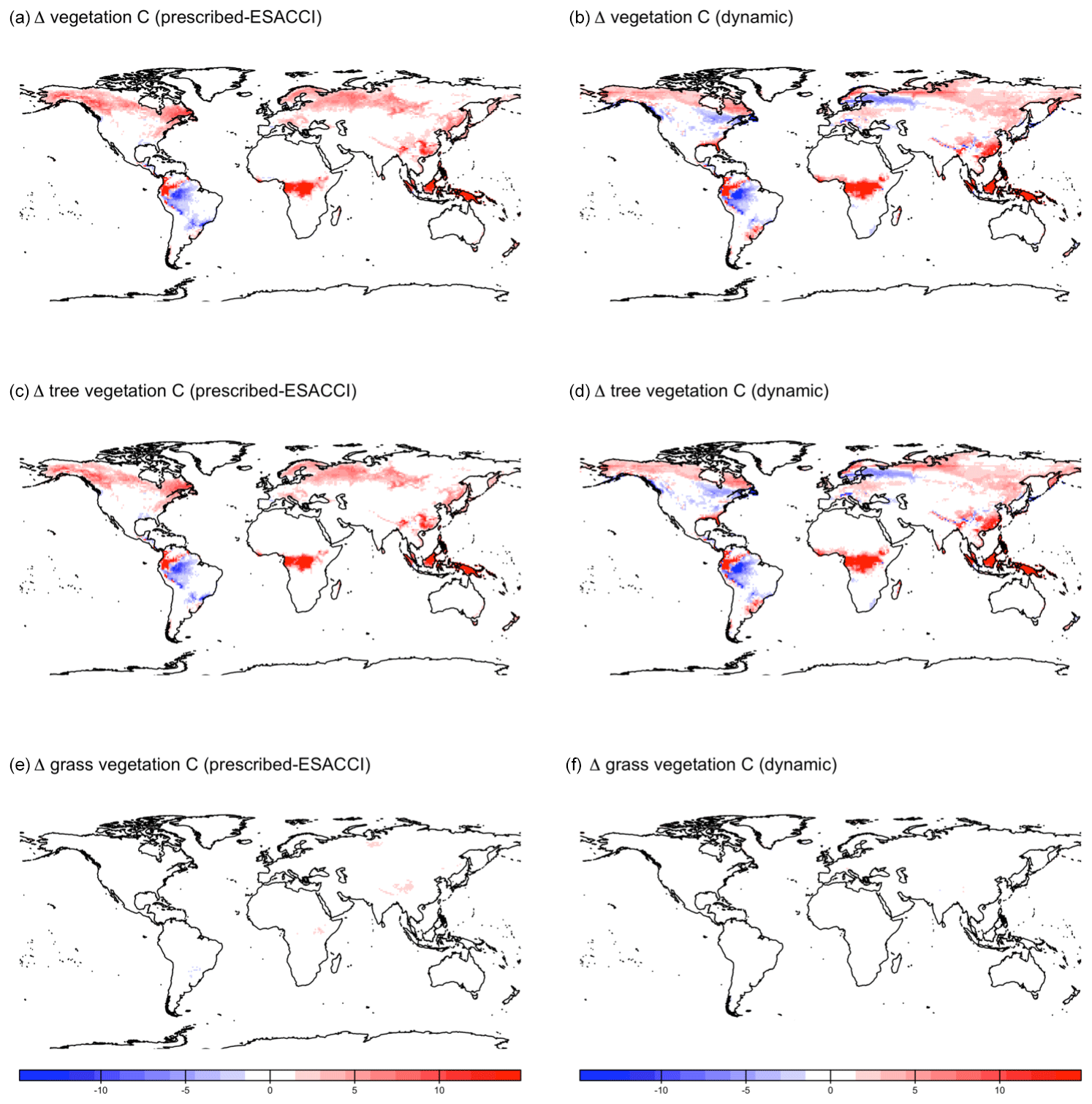
Figure B8Change in vegetation C simulated by CLASSIC with prescribed land cover (with an ESACCI-derived land cover forcing) and CLASSIC with dynamic land cover for SSP5-8.5 (2015–2100). (a, b) Total vegetation C, (c, d) tree vegetation C, and (e, f) grass vegetation C. Differences reflect the change between the average over 1995–2015 and 2080–2100.
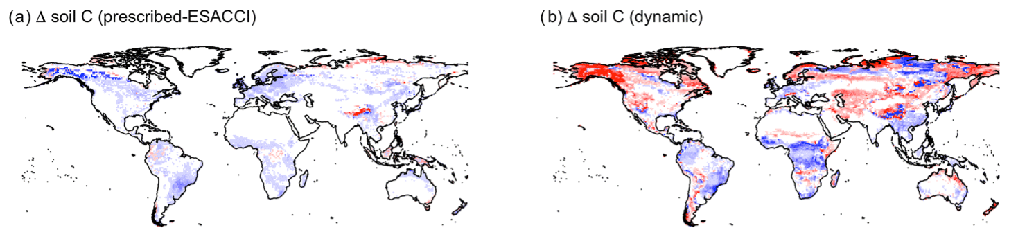
Figure B9Change in soil C simulated by (a) CLASSIC with prescribed land cover (with an ESACCI-derived land cover forcing) and (b) CLASSIC with dynamic land cover for SSP5-8.5 (2015–2100). Differences reflect the change between the average over 1995–2015 and 2080–2100.
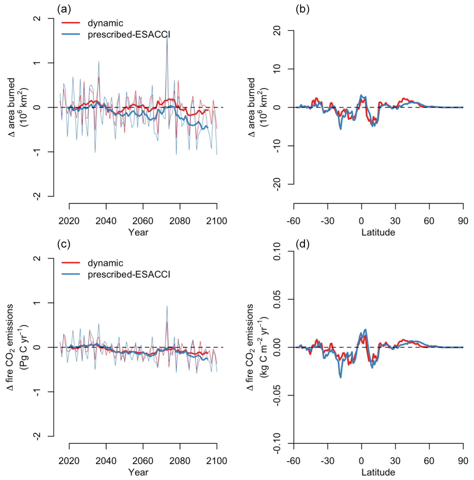
Figure B10Change in (a, b) area burned and (c, d) fire CO2 emissions by CLASSIC with prescribed land cover (with an ESACCI-derived land cover forcing) and CLASSIC with dynamic land cover for SSP5-8.5 (2015–2100). For the latitudinal distributions, CLASSIC simulations were averaged over 2080–2100. Thin lines indicate the annual value, and thick lines indicate the moving average over 10 years.
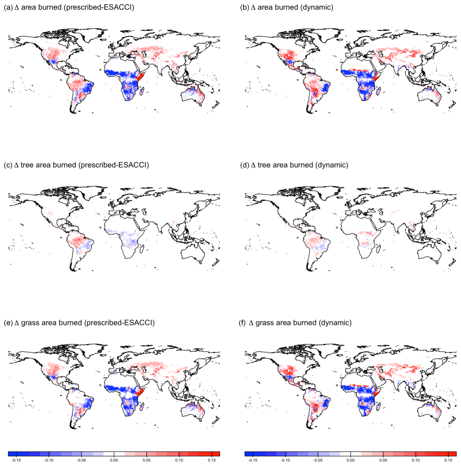
Figure B11Change in area burned simulated by CLASSIC with prescribed land cover (with an ESACCI-derived land cover forcing) and CLASSIC with dynamic land cover for SSP5-8.5 (2015–2100). (a, b) Total area burned, (c, d) tree area burned, and (e, f) grass area burned. Differences reflect the change between the average over 1995–2015 and 2080–2100.
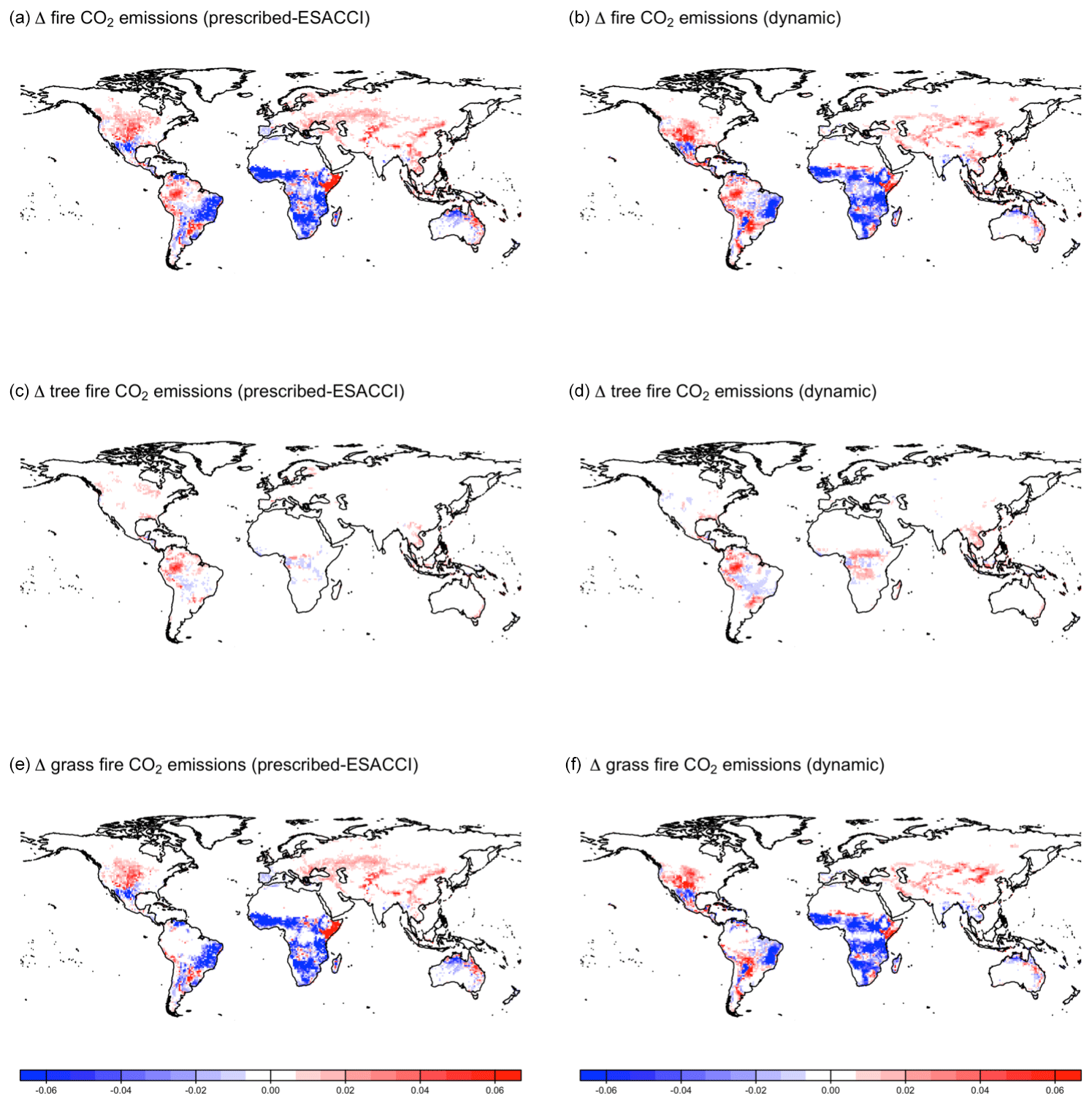
Figure B12Change in fire CO2 emissions simulated by CLASSIC with prescribed land cover (with an ESACCI-derived land cover forcing) and CLASSIC with dynamic land cover for SSP5-8.5 (2015–2100). (a, b) Total fire CO2 emissions, (c, d) tree fire CO2 emissions, and (e, f) grass fire CO2 emissions. Differences reflect the change between the average over 1995–2015 and 2080–2100.
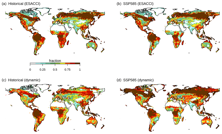
Figure B13Natural vegetation fraction per grid cell (a, b) in the ESACCI-derived land cover product and (c, d) simulated by CLASSIC with dynamic land cover over (a, c) the historical period (averaged over 1995–2015) and (b, d) for SSP5-8.5 (averaged over 2080–2100).
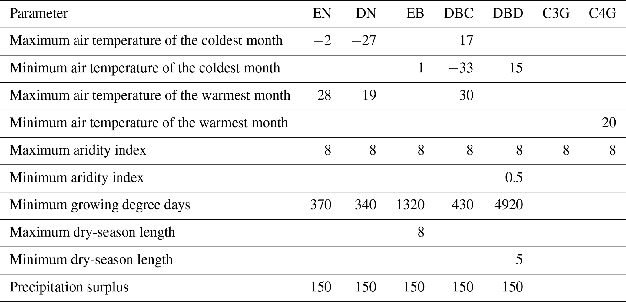
Table B2Observation-based datasets used in AMBER. Described in detail in Seiler et al. (2022). Datasets are globally gridded or in situ (specified).
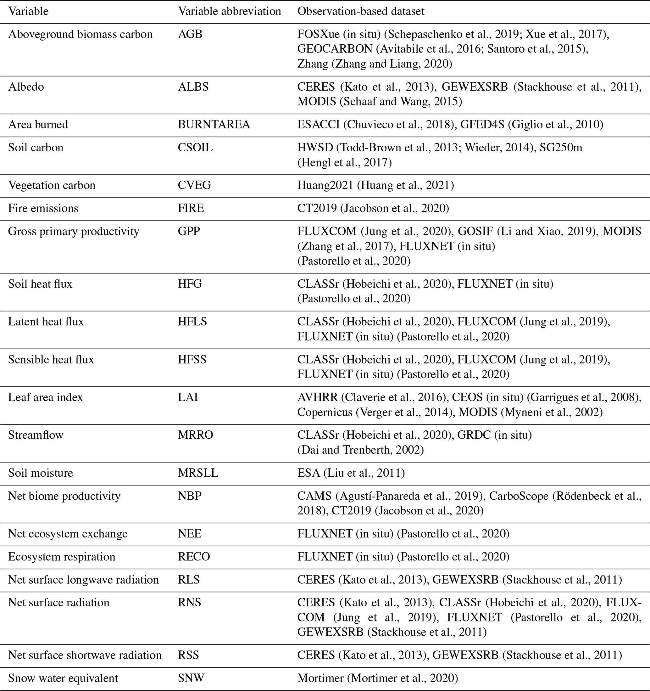
Table B3Parameters associated with the calculation of colonisation and mortality rates for each PFT.
The source code for CLASSIC is available on the CLASSIC community Zenodo page (https://zenodo.org/communities/classic?q&l=list&p=1&s=10&sort=newest, Melton et al., 2019). AMBER is available at https://gitlab.com/cseiler/AMBER (Seiler, 2024).
The model outputs are available at Zenodo (https://doi.org/10.5281/zenodo.11520769, Kou-Giesbrecht, 2024).
SKG designed and conducted the study and prepared the initial manuscript. VKA provided input on the study design and the initial manuscript. CS and LW provided input on the subsequent revisions.
The contact author has declared that none of the authors has any competing interests.
Publisher’s note: Copernicus Publications remains neutral with regard to jurisdictional claims made in the text, published maps, institutional affiliations, or any other geographical representation in this paper. While Copernicus Publications makes every effort to include appropriate place names, the final responsibility lies with the authors.
The authors would like to thank the CLASSIC team for their input (Paul Bartlett, Mike Brady, Ed Chan, Salvatore Curasi, Joe Melton, and Gesa Meyer).
This paper was edited by Xi Yang and reviewed by two anonymous referees.
Agustí-Panareda, A., Diamantakis, M., Massart, S., Chevallier, F., Muñoz-Sabater, J., Barré, J., Curcoll, R., Engelen, R., Langerock, B., Law, R. M., Loh, Z., Morguí, J. A., Parrington, M., Peuch, V.-H., Ramonet, M., Roehl, C., Vermeulen, A. T., Warneke, T., and Wunch, D.: Modelling CO2 weather – why horizontal resolution matters, Atmos. Chem. Phys., 19, 7347–7376, https://doi.org/10.5194/acp-19-7347-2019, 2019.
Aleixo, I., Norris, D., Hemerik, L., Barbosa, A., Prata, E., Costa, F., and Poorter, L.: Amazonian rainforest tree mortality driven by climate and functional traits, Nat. Clim. Change, 9, 384–388, https://doi.org/10.1038/s41558-019-0458-0, 2019.
Alo, C. A. and Wang, G.: Potential future changes of the terrestrial ecosystem based on climate projections by eight general circulation models, J. Geophys. Res.-Biogeo., 113, G01004, https://doi.org/10.1029/2007JG000528, 2008.
Arora, V. K. and Boer, G. J.: A parameterization of leaf phenology for the terrestrial ecosystem component of climate models, Glob. Change Biol., 11, 39–59, https://doi.org/10.1111/j.1365-2486.2004.00890.x, 2005a.
Arora, V. K. and Boer, G. J.: Fire as an interactive component of dynamic vegetation models, J. Geophys. Res.-Biogeo., 110, G02008, https://doi.org/10.1029/2005jg000042, 2005b.
Arora, V. K. and Boer, G. J.: Simulating Competition and Coexistence between Plant Functional Types in a Dynamic Vegetation Model, Earth Interact., 10, 1–30, https://doi.org/10.1175/EI170.1, 2006.
Arora, V. K. and Melton, J. R.: Reduction in global area burned and wildfire emissions since 1930s enhances carbon uptake by land, Nat. Commun., 9, 1–10, https://doi.org/10.1038/s41467-018-03838-0, 2018.
Arora, V. K., Katavouta, A., Williams, R. G., Jones, C. D., Brovkin, V., Friedlingstein, P., Schwinger, J., Bopp, L., Boucher, O., Cadule, P., Chamberlain, M. A., Christian, J. R., Delire, C., Fisher, R. A., Hajima, T., Ilyina, T., Joetzjer, E., Kawamiya, M., Koven, C. D., Krasting, J. P., Law, R. M., Lawrence, D. M., Lenton, A., Lindsay, K., Pongratz, J., Raddatz, T., Séférian, R., Tachiiri, K., Tjiputra, J. F., Wiltshire, A., Wu, T., and Ziehn, T.: Carbon–concentration and carbon–climate feedbacks in CMIP6 models and their comparison to CMIP5 models, Biogeosciences, 17, 4173–4222, https://doi.org/10.5194/bg-17-4173-2020, 2020.
Arora, V. K., Seiler, C., Wang, L., and Kou-Giesbrecht, S.: Towards an ensemble-based evaluation of land surface models in light of uncertain forcings and observations, Biogeosciences, 20, 1313–1355, https://doi.org/10.5194/bg-20-1313-2023, 2023.
Asaadi, A. and Arora, V. K.: Implementation of nitrogen cycle in the CLASSIC land model, Biogeosciences, 18, 669–706, https://doi.org/10.5194/bg-18-669-2021, 2021.
Asaadi, A., Arora, V. K., Melton, J. R., and Bartlett, P.: An improved parameterization of leaf area index (LAI) seasonality in the Canadian Land Surface Scheme (CLASS) and Canadian Terrestrial Ecosystem Model (CTEM) modelling framework, Biogeosciences, 15, 6885–6907, https://doi.org/10.5194/bg-15-6885-2018, 2018.
Avitabile, V., Herold, M., Heuvelink, G. B. M., Lewis, S. L., Phillips, O. L., Asner, G. P., Armston, J., Ashton, P. S., Banin, L., Bayol, N., Berry, N. J., Boeckx, P., de Jong, B. H. J., DeVries, B., Girardin, C. A. J., Kearsley, E., Lindsell, J. A., Lopez-Gonzalez, G., Lucas, R., Malhi, Y., Morel, A., Mitchard, E. T. A., Nagy, L., Qie, L., Quinones, M. J., Ryan, C. M., Ferry, S. J. W., Sunderland, T., Laurin, G. V., Gatti, R. C., Valentini, R., Verbeeck, H., Wijaya, A., and Willcock, S.: An integrated pan-tropical biomass map using multiple reference datasets, Glob. Change Biol., 22, 1406–1420, https://doi.org/10.1111/gcb.13139, 2016.
Baltzer, J. L., Day, N. J., Walker, X. J., Greene, D., Mack, M. C., Alexander, H. D., Arseneault, D., Barnes, J., Bergeron, Y., Boucher, Y., Bourgeau-Chavez, L., Brown, C. D., Carrière, S., Howard, B. K., Gauthier, S., Parisien, M.-A., Reid, K. A., Rogers, B. M., Roland, C., Sirois, L., Stehn, S., Thompson, D. K., Turetsky, M. R., Veraverbeke, S., Whitman, E., Yang, J., and Johnstone, J. F.: Increasing fire and the decline of fire adapted black spruce in the boreal forest, P. Natl. Acad. Sci. USA, 118, e2024872118, https://doi.org/10.1073/pnas.2024872118, 2021.
Bartholomé, E. and Belward, A. S.: GLC2000: a new approach to global land cover mapping from Earth observation data, Int. J. Remote Sens., 26, 1959–1977, https://doi.org/10.1080/01431160412331291297, 2005.
Box, E. O.: Plant functional types and climate at the global scale, J. Veg. Sci., 7, 309–320, 1996.
Braghiere, R. K., Fisher, J. B., Miner, K. R., Miller, C. E., Worden, J. R., Schimel, D. S., and Frankenberg, C.: Tipping point in North American Arctic-Boreal carbon sink persists in new generation Earth system models despite reduced uncertainty, Environ. Res. Lett., 18, 025008, https://doi.org/10.1088/1748-9326/acb226, 2023.
Brandt, M., Mbow, C., Diouf, A. A., Verger, A., Samimi, C., and Fensholt, R.: Ground- and satellite-based evidence of the biophysical mechanisms behind the greening Sahel, Glob. Change Biol., 21, 1610–1620, https://doi.org/10.1111/gcb.12807, 2015.
Chapin, F. S., Sturm, M., Serreze, M. C., McFadden, J. P., Key, J. R., Lloyd, A. H., McGuire, A. D., Rupp, T. S., Lynch, A. H., Schimel, J. P., Beringer, J., Chapman, W. L., Epstein, H. E., Euskirchen, E. S., Hinzman, L. D., Jia, G., Ping, C.-L., Tape, K. D., Thompson, C. D. C., Walker, D. A., and Welker, J. M.: Role of Land-Surface Changes in Arctic Summer Warming, Science, 310, 657–660, https://doi.org/10.1126/science.1117368, 2005.
Chen, I.-C., Hill, J. K., Ohlemüller, R., Roy, D. B., and Thomas, C. D.: Rapid Range Shifts of Species Associated with High Levels of Climate Warming, Science, 333, 1024–1026, https://doi.org/10.1126/science.1206432, 2011.
Chini, L., Hurtt, G., Sahajpal, R., Frolking, S., Goldewijk, K. K., Sitch, S., Ganzenmüller, R., Ma, L., Ott, L., Pongratz, J., and Poulter, B.: Land-use harmonization datasets for annual global carbon budgets, Earth Sy. Sci. Data, 13, 4175–4189, https://doi.org/10.5194/essd-13-4175-2021, 2021.
Chuvieco, E., Lizundia-Loiola, J., Pettinari, M. L., Ramo, R., Padilla, M., Tansey, K., Mouillot, F., Laurent, P., Storm, T., Heil, A., and Plummer, S.: Generation and analysis of a new global burned area product based on MODIS 250m reflectance bands and thermal anomalies, Earth Sy. Sci. Data, 10, 2015–2031, https://doi.org/10.5194/essd-10-2015-2018, 2018.
Claverie, M., Matthews, J. L., Vermote, E. F., and Justice, C. O.: A 30+ Year AVHRR LAI and FAPAR Climate Data Record: Algorithm Description and Validation, Remote Sens., 8, 263, https://doi.org/10.3390/rs8030263, 2016.
Collier, N., Hoffman, F. M., Lawrence, D. M., Keppel-Aleks, G., Koven, C. D., Riley, W. J., Mu, M., and Randerson, J. T.: The International Land Model Benchmarking (ILAMB) System: Design, Theory, and Implementation, J. Adv. Model. Earth Sy., 10, 2731–2754, https://doi.org/10.1029/2018MS001354, 2018.
Corlett, R. T. and Westcott, D. A.: Will plant movements keep up with climate change?, Trend. Ecol. Evol., 28, 482–488, https://doi.org/10.1016/j.tree.2013.04.003, 2013.
Dai, A. and Trenberth, K. E.: Estimates of Freshwater Discharge from Continents: Latitudinal and Seasonal Variations, J. Hydrometeorol., 3, 660–687, https://doi.org/10.1175/1525-7541(2002)003<0660:EOFDFC>2.0.CO;2, 2002.
Davidson, E. A., de Araújo, A. C., Artaxo, P., Balch, J. K., Brown, I. F., C. Bustamante, M. M., Coe, M. T., DeFries, R. S., Keller, M., Longo, M., Munger, J. W., Schroeder, W., Soares-Filho, B. S., Souza, C. M., and Wofsy, S. C.: The Amazon basin in transition, Nature, 481, 321–328, https://doi.org/10.1038/nature10717, 2012.
Defourny, P., Lamarche, C., Brockmann, C., Boettcher, M., Bontemps, S., De Maet, T., Duveiller, G. L. Harper, K., Hartley A., Kirches, G., Moreau, I., Peylin, P., Ottlé, C., Radoux J., Van Bogaert, E., Ramoino, F., Albergel, C., and Arino, O.: Observed annual global land-use change from 1992 to 2020 three times more dynamic than reported by inventory-based statistics, in preparation, http://maps.elie.ucl.ac.be/CCI/viewer/download.php (Last access: 2017), 2023.
Dusenge, M. E., Duarte, A. G., and Way, D. A.: Plant carbon metabolism and climate change: elevated CO2 and temperature impacts on photosynthesis, photorespiration and respiration, New Phytol., 221, 32–49, 2019.
Elmendorf, S. C., Henry, G. H. R., Hollister, R. D., Björk, R. G., Boulanger-Lapointe, N., Cooper, E. J., Cornelissen, J. H. C., Day, T. A., Dorrepaal, E., Elumeeva, T. G., Gill, M., Gould, W. A., Harte, J., Hik, D. S., Hofgaard, A., Johnson, D. R., Johnstone, J. F., Jónsdóttir, I. S., Jorgenson, J. C., Klanderud, K., Klein, J. A., Koh, S., Kudo, G., Lara, M., Lévesque, E., Magnússon, B., May, J. L., Mercado-Díaz, J. A., Michelsen, A., Molau, U., Myers-Smith, I. H., Oberbauer, S. F., Onipchenko, V. G., Rixen, C., Martin Schmidt, N., Shaver, G. R., Spasojevic, M. J., Þórhallsdóttir, Þ. E., Tolvanen, A., Troxler, T., Tweedie, C. E., Villareal, S., Wahren, C.-H., Walker, X., Webber, P. J., Welker, J. M., and Wipf, S.: Plot-scale evidence of tundra vegetation change and links to recent summer warming, Nat. Clim. Change, 2, 453–457, https://doi.org/10.1038/nclimate1465, 2012.
Fisher, R. A. and Koven, C. D.: Perspectives on the Future of Land Surface Models and the Challenges of Representing Complex Terrestrial Systems, J. Adv. Model. Earth Sy., 12, e2018MS001453, https://doi.org/10.1029/2018MS001453, 2020.
Friedl, M. A., Sulla-Menashe, D., Tan, B., Schneider, A., Ramankutty, N., Sibley, A., and Huang, X.: MODIS Collection 5 global land cover: Algorithm refinements and characterization of new datasets, Remote Sens. Environ., 114, 168–182, https://doi.org/10.1016/j.rse.2009.08.016, 2010.
Friedlingstein, P., O'Sullivan, M., Jones, M. W., Andrew, R. M., Gregor, L., Hauck, J., Le Quéré, C., Luijkx, I. T., Olsen, A., Peters, G. P., Peters, W., Pongratz, J., Schwingshackl, C., Sitch, S., Canadell, J. G., Ciais, P., Jackson, R. B., Alin, S. R., Alkama, R., Arneth, A., Arora, V. K., Bates, N. R., Becker, M., Bellouin, N., Bittig, H. C., Bopp, L., Chevallier, F., Chini, L. P., Cronin, M., Evans, W., Falk, S., Feely, R. A., Gasser, T., Gehlen, M., Gkritzalis, T., Gloege, L., Grassi, G., Gruber, N., Gürses, Ö., Harris, I., Hefner, M., Houghton, R. A., Hurtt, G. C., Iida, Y., Ilyina, T., Jain, A. K., Jersild, A., Kadono, K., Kato, E., Kennedy, D., Klein Goldewijk, K., Knauer, J., Korsbakken, J. I., Landschützer, P., Lefèvre, N., Lindsay, K., Liu, J., Liu, Z., Marland, G., Mayot, N., McGrath, M. J., Metzl, N., Monacci, N. M., Munro, D. R., Nakaoka, S.-I., Niwa, Y., O'Brien, K., Ono, T., Palmer, P. I., Pan, N., Pierrot, D., Pocock, K., Poulter, B., Resplandy, L., Robertson, E., Rödenbeck, C., Rodriguez, C., Rosan, T. M., Schwinger, J., Séférian, R., Shutler, J. D., Skjelvan, I., Steinhoff, T., Sun, Q., Sutton, A. J., Sweeney, C., Takao, S., Tanhua, T., Tans, P. P., Tian, X., Tian, H., Tilbrook, B., Tsujino, H., Tubiello, F., van der Werf, G. R., Walker, A. P., Wanninkhof, R., Whitehead, C., Willstrand Wranne, A., Wright, R., Yuan, W., Yue, C., Yue, X., Zaehle, S., Zeng, J., and Zheng, B.: Global Carbon Budget 2022, Earth Syst. Sci. Data, 14, 4811–4900, https://doi.org/10.5194/essd-14-4811-2022, 2022.
Garrigues, S., Lacaze, R., Baret, F., Morisette, J. T., Weiss, M., Nickeson, J. E., Fernandes, R., Plummer, S., Shabanov, N. V., Myneni, R. B., Knyazikhin, Y., and Yang, W.: Validation and intercomparison of global Leaf Area Index products derived from remote sensing data, J. Geophys. Res.-Biogeo., 113, G02028, https://doi.org/10.1029/2007JG000635, 2008.
Giglio, L., Randerson, J. T., van der Werf, G. R., Kasibhatla, P. S., Collatz, G. J., Morton, D. C., and DeFries, R. S.: Assessing variability and long-term trends in burned area by merging multiple satellite fire products, Biogeosciences, 7, 1171–1186, https://doi.org/10.5194/bg-7-1171-2010, 2010.
Harris, I., Osborn, T. J., Jones, P., and Lister, D.: Version 4 of the CRU TS monthly high-resolution gridded multivariate climate dataset, Sci. Data, 7, 1–18, https://doi.org/10.1038/s41597-020-0453-3, 2020.
Hartley, A. J., MacBean, N., Georgievski, G., and Bontemps, S.: Uncertainty in plant functional type distributions and its impact on land surface models, Remote Sens. Environ., 203, 71–89, https://doi.org/10.1016/j.rse.2017.07.037, 2017.
Hengl, T., De Jesus, J. M., Heuvelink, G. B. M., Gonzalez, M. R., Kilibarda, M., Blagotić, A., Shangguan, W., Wright, M. N., Geng, X., Bauer-Marschallinger, B., Guevara, M. A., Vargas, R., MacMillan, R. A., Batjes, N. H., Leenaars, J. G. B., Ribeiro, E., Wheeler, I., Mantel, S., and Kempen, B.: SoilGrids250m: Global gridded soil information based on machine learning, PLoS ONE, 12, e0169748, https://doi.org/10.1371/journal.pone.0169748, 2017.
Herrmann, S. M., Anyamba, A., and Tucker, C. J.: Recent trends in vegetation dynamics in the African Sahel and their relationship to climate, Glob. Environ. Change, 15, 394–404, https://doi.org/10.1016/j.gloenvcha.2005.08.004, 2005.
Hisano, M., Ryo, M., Chen, X., and Chen, H. Y. H.: Rapid functional shifts across high latitude forests over the last 65 years, Glob. Change Biol., 27, 3846–3858, https://doi.org/10.1111/gcb.15710, 2021.
Hobeichi, S., Abramowitz, G., and Evans, J.: Conserving Land–Atmosphere Synthesis Suite (CLASS), J. Clim., 33, 1821–1844, https://doi.org/10.1175/JCLI-D-19-0036.1, 2020.
Houghton, R. A., House, J. I., Pongratz, J., van der Werf, G. R., DeFries, R. S., Hansen, M. C., Le Quéré, C., and Ramankutty, N.: Carbon emissions from land use and land-cover change, Biogeosciences, 9, 5125–5142, https://doi.org/10.5194/bg-9-5125-2012, 2012.
Huang, K., Xia, J., Wang, Y., Ahlström, A., Chen, J., Cook, R. B., Cui, E., Fang, Y., Fisher, J. B., Huntzinger, D. N., Li, Z., Michalak, A. M., Qiao, Y., Schaefer, K., Schwalm, C., Wang, J., Wei, Y., Xu, X., Yan, L., Bian, C., and Luo, Y.: Enhanced peak growth of global vegetation and its key mechanisms, Nat. Ecol. Evol., 2, 1897–1905, https://doi.org/10.1038/s41559-018-0714-0, 2018.
Huang, Y., Ciais, P., Santoro, M., Makowski, D., Chave, J., Schepaschenko, D., Abramoff, R. Z., Goll, D. S., Yang, H., Chen, Y., Wei, W., and Piao, S.: A global map of root biomass across the world's forests, Earth Syst. Sci. Data, 13, 4263–4274, https://doi.org/10.5194/essd-13-4263-2021, 2021.
Hurtt, G. C., Chini, L., Sahajpal, R., Frolking, S., Bodirsky, B. L., Calvin, K., Doelman, J. C., Fisk, J., Fujimori, S., Klein Goldewijk, K., Hasegawa, T., Havlik, P., Heinimann, A., Humpenöder, F., Jungclaus, J., Kaplan, J. O., Kennedy, J., Krisztin, T., Lawrence, D., Lawrence, P., Ma, L., Mertz, O., Pongratz, J., Popp, A., Poulter, B., Riahi, K., Shevliakova, E., Stehfest, E., Thornton, P., Tubiello, F. N., van Vuuren, D. P., and Zhang, X.: Harmonization of global land use change and management for the period 850–2100 (LUH2) for CMIP6, Geosci. Model Dev., 13, 5425–5464, https://doi.org/10.5194/gmd-13-5425-2020, 2020.
Jacobson, A. R., Schuldt, K. N., Miller, J. B., Oda, T., Tans, P., Andrews, A., Mund, J., Ott, L., Collatz, G. J., and Aalto, T.: Carbontracker ct2019, NOAA Earth system research laboratory, global monitoring division, https://doi.org/10.25925/39M3-6069, 2020.
Johnstone, J. F. and Chapin, F. S.: Effects of Soil Burn Severity on Post-Fire Tree Recruitment in Boreal Forest, Ecosystems, 9, 14–31, https://doi.org/10.1007/s10021-004-0042-x, 2006.
Jung, M., Koirala, S., Weber, U., Ichii, K., Gans, F., Camps-Valls, G., Papale, D., Schwalm, C., Tramontana, G., and Reichstein, M.: The FLUXCOM ensemble of global land-atmosphere energy fluxes, Sci. Data, 6, 74, https://doi.org/10.1038/s41597-019-0076-8, 2019.
Jung, M., Schwalm, C., Migliavacca, M., Walther, S., Camps-Valls, G., Koirala, S., Anthoni, P., Besnard, S., Bodesheim, P., Carvalhais, N., Chevallier, F., Gans, F., Goll, D. S., Haverd, V., Köhler, P., Ichii, K., Jain, A. K., Liu, J., Lombardozzi, D., Nabel, J. E. M. S., Nelson, J. A., O'Sullivan, M., Pallandt, M., Papale, D., Peters, W., Pongratz, J., Rödenbeck, C., Sitch, S., Tramontana, G., Walker, A., Weber, U., and Reichstein, M.: Scaling carbon fluxes from eddy covariance sites to globe: synthesis and evaluation of the FLUXCOM approach, Biogeosciences, 17, 1343–1365, https://doi.org/10.5194/bg-17-1343-2020, 2020.
Kato, S., Loeb, N. G., Rose, F. G., Doelling, D. R., Rutan, D. A., Caldwell, T. E., Yu, L., and Weller, R. A.: Surface Irradiances Consistent with CERES-Derived Top-of-Atmosphere Shortwave and Longwave Irradiances, J. Clim., 26, 2719–2740, https://doi.org/10.1175/JCLI-D-12-00436.1, 2013.
Klein Goldewijk, K., Beusen, A., Doelman, J., and Stehfest, E.: Anthropogenic land use estimates for the Holocene – HYDE 3.2, Earth Syst. Sci. Data, 9, 927–953, https://doi.org/10.5194/essd-9-927-2017, 2017.
Kou-Giesbrecht, S.: The impacts of modelling prescribed vs. dynamic land cover in a high CO2 future scenario – greening of the Arctic and Amazonian dieback, Zenodo [data set], https://doi.org/10.5281/zenodo.11520769, 2024.
Kou-Giesbrecht, S. and Arora, V. K.: Representing the Dynamic Response of Vegetation to Nitrogen Limitation via Biological Nitrogen Fixation in the CLASSIC Land Model, Global Biogeochem. Cy., 36, e2022GB007341, https://doi.org/10.1029/2022GB007341, 2022.
Koven, C. D., Arora, V. K., Cadule, P., Fisher, R. A., Jones, C. D., Lawrence, D. M., Lewis, J., Lindsay, K., Mathesius, S., Meinshausen, M., Mills, M., Nicholls, Z., Sanderson, B. M., Séférian, R., Swart, N. C., Wieder, W. R., and Zickfeld, K.: Multi-century dynamics of the climate and carbon cycle under both high and net negative emissions scenarios, Earth Syst. Dynam., 13, 885–909, https://doi.org/10.5194/esd-13-885-2022, 2022.
Lan, X., Tans, P., and Thoning, K. W.: Trends in globally-averaged CO2 determined from NOAA Global Monitoring Laboratory measurements, Version 2024-07, https://doi.org/10.15138/9N0H-ZH07, 2024.
Lange, S. and Büchner, M.: ISIMIP3b bias-adjusted atmospheric climate input data (v1.1), ISIMIP Repository [data set], https://doi.org/10.48364/ISIMIP.842396.1, 2021.
Lenoir, J. and Svenning, J.: Climate-related range shifts – a global multidimensional synthesis and new research directions, Ecography, 38, 15–28, 2015.
Li, X. and Xiao, J.: Mapping Photosynthesis Solely from Solar-Induced Chlorophyll Fluorescence: A Global, Fine-Resolution Dataset of Gross Primary Production Derived from OCO-2, Remote Sens., 11, 2563, https://doi.org/10.3390/rs11212563, 2019.
Liu, Y. Y., Parinussa, R. M., Dorigo, W. A., De Jeu, R. A. M., Wagner, W., van Dijk, A. I. J. M., McCabe, M. F., and Evans, J. P.: Developing an improved soil moisture dataset by blending passive and active microwave satellite-based retrievals, Hydrol. Earth Syst. Sci., 15, 425–436, https://doi.org/10.5194/hess-15-425-2011, 2011.
Luo, X., Zhou, H., Satriawan, T. W., Tian, J., Zhao, R., Keenan, T. F., Griffith, D. M., Sitch, S., Smith, N. G., and Still, C. J.: Mapping the global distribution of C4 vegetation using observations and optimality theory, Nat. Commun., 15, 1219, https://doi.org/10.1038/s41467-024-45606-3, 2024.
Macander, M. J., Nelson, P. R., Nawrocki, T. W., Frost, G. V., Orndahl, K. M., Palm, E. C., Wells, A. F., and Goetz, S. J.: Time-series maps reveal widespread change in plant functional type cover across Arctic and boreal Alaska and Yukon, Environ. Res. Lett., 17, 054042, https://doi.org/10.1088/1748-9326/ac6965, 2022.
Mack, M. C., Walker, X. J., Johnstone, J. F., Alexander, H. D., Melvin, A. M., Jean, M., and Miller, S. N.: Carbon loss from boreal forest wildfires offset by increased dominance of deciduous trees, Science, 372, 280–283, https://doi.org/10.1126/science.abf3903, 2021.
Malhi, Y., Roberts, J. T., Betts, R. A., Killeen, T. J., Li, W., and Nobre, C. A.: Climate Change, Deforestation, and the Fate of the Amazon, Science, 319, 169–172, https://doi.org/10.1126/science.1146961, 2008.
Melton, J. R. and Arora, V. K.: Competition between plant functional types in the Canadian Terrestrial Ecosystem Model (CTEM) v. 2.0, Geosci. Model Dev., 9, 323–361, https://doi.org/10.5194/gmd-9-323-2016, 2016.
Melton, J. R., Shrestha, R. K., and Arora, V. K.: The influence of soils on heterotrophic respiration exerts a strong control on net ecosystem productivity in seasonally dry Amazonian forests, Biogeosciences, 12, 1151–1168, https://doi.org/10.5194/bg-12-1151-2015, 2015.
Melton, J. R., Arora, V. K., Wisernig-Cojoc, E., Seiler, C., Fortier, M., Chan, E., and Teckentrup, L.: CLASSIC v1.0: The open-source community successor to the Canadian Land Surface Scheme (CLASS) and the Canadian Terrestrial Ecosystem Model (CTEM)-Part 1: Model framework and site-level performance, Geosci. Model Dev., 13, 2825–2850, https://doi.org/10.5194/gmd-13-2825-2020, 2020.
Melton, J. R., Arora, V., Wisernig-Cojoc, E., Seiler, C., Fortier, M., Chan, E., and Teckentrup, L.: The Canadian Land Surface Scheme including Biogeochemical Cycles (1.0), Zenodo [code], https://doi.org/10.5281/zenodo.3522407, 2019.
Monerie, P.-A., Wainwright, C. M., Sidibe, M., and Akinsanola, A. A.: Model uncertainties in climate change impacts on Sahel precipitation in ensembles of CMIP5 and CMIP6 simulations, Clim. Dynam., 55, 1385–1401, https://doi.org/10.1007/s00382-020-05332-0, 2020.
Mortimer, C., Mudryk, L., Derksen, C., Luojus, K., Brown, R., Kelly, R., and Tedesco, M.: Evaluation of long-term Northern Hemisphere snow water equivalent products, The Cryosphere, 14, 1579–1594, https://doi.org/10.5194/tc-14-1579-2020, 2020.
Myers-Smith, I. H., Kerby, J. T., Phoenix, G. K., Bjerke, J. W., Epstein, H. E., Assmann, J. J., John, C., Andreu-Hayles, L., Angers-Blondin, S., Beck, P. S. A., Berner, L. T., Bhatt, U. S., Bjorkman, A. D., Blok, D., Bryn, A., Christiansen, C. T., Cornelissen, J. H. C., Cunliffe, A. M., Elmendorf, S. C., Forbes, B. C., Goetz, S. J., Hollister, R. D., de Jong, R., Loranty, M. M., Macias-Fauria, M., Maseyk, K., Normand, S., Olofsson, J., Parker, T. C., Parmentier, F.-J. W., Post, E., Schaepman-Strub, G., Stordal, F., Sullivan, P. F., Thomas, H. J. D., Tømmervik, H., Treharne, R., Tweedie, C. E., Walker, D. A., Wilmking, M., and Wipf, S.: Complexity revealed in the greening of the Arctic, Nat. Clim. Change, 10, 106–117, https://doi.org/10.1038/s41558-019-0688-1, 2020.
Myneni, R. B., Hoffman, S., Knyazikhin, Y., Privette, J. L., Glassy, J., Tian, Y., Wang, Y., Song, X., Zhang, Y., Smith, G. R., Lotsch, A., Friedl, M., Morisette, J. T., Votava, P., Nemani, R. R., and Running, S. W.: Global products of vegetation leaf area and fraction absorbed PAR from year one of MODIS data, Remote Sens. Environ., 83, 214–231, https://doi.org/10.1016/S0034-4257(02)00074-3, 2002.
National Research Council: Earth observations from space: The first 50 years of scientific achievements, National Academies Press, https://doi.org/10.17226/11991, 2008.
Olsson, L., Eklundh, L., and Ardö, J.: A recent greening of the Sahel – trends, patterns and potential causes, J. Arid Environ., 63, 556–566, https://doi.org/10.1016/j.jaridenv.2005.03.008, 2005.
Parry, I. M., Ritchie, P. D. L., and Cox, P. M.: Evidence of localised Amazon rainforest dieback in CMIP6 models, Earth Syst. Dynam., 13, 1667–1675, https://doi.org/10.5194/esd-13-1667-2022, 2022.
Pastorello, G., Trotta, C., Canfora, E., et al.: The FLUXNET2015 dataset and the ONEFlux processing pipeline for eddy covariance data, Sci. Data, 7, 225, https://doi.org/10.1038/s41597-020-0534-3, 2020.
Pearson, R. G., Phillips, S. J., Loranty, M. M., Beck, P. S. A., Damoulas, T., Knight, S. J., and Goetz, S. J.: Shifts in Arctic vegetation and associated feedbacks under climate change, Nat. Clim. Change, 3, 673–677, https://doi.org/10.1038/nclimate1858, 2013.
Pecl, G. T., Araújo, M. B., Bell, J. D., Blanchard, J., Bonebrake, T. C., Chen, I.-C., Clark, T. D., Colwell, R. K., Danielsen, F., and Evengård, B.: Biodiversity redistribution under climate change: Impacts on ecosystems and human well-being, Science, 355, eaai9214, https://doi.org/10.1126/science.aai9214, 2017.
Phillips, O. L., Aragão, L. E. O. C., Lewis, S. L., Fisher, J. B., Lloyd, J., López-González, G., Malhi, Y., Monteagudo, A., Peacock, J., Quesada, C. A., van der Heijden, G., Almeida, S., Amaral, I., Arroyo, L., Aymard, G., Baker, T. R., Bánki, O., Blanc, L., Bonal, D., Brando, P., Chave, J., de Oliveira, Á. C. A., Cardozo, N. D., Czimczik, C. I., Feldpausch, T. R., Freitas, M. A., Gloor, E., Higuchi, N., Jiménez, E., Lloyd, G., Meir, P., Mendoza, C., Morel, A., Neill, D. A., Nepstad, D., Patiño, S., Peñuela, M. C., Prieto, A., Ramírez, F., Schwarz, M., Silva, J., Silveira, M., Thomas, A. S., Steege, H. ter, Stropp, J., Vásquez, R., Zelazowski, P., Dávila, E. A., Andelman, S., Andrade, A., Chao, K.-J., Erwin, T., Di Fiore, A., C., E. H., Keeling, H., Killeen, T. J., Laurance, W. F., Cruz, A. P., Pitman, N. C. A., Vargas, P. N., Ramírez-Angulo, H., Rudas, A., Salamão, R., Silva, N., Terborgh, J., and Torres-Lezama, A.: Drought Sensitivity of the Amazon Rainforest, Science, 323, 1344–1347, https://doi.org/10.1126/science.1164033, 2009.
Piao, S., Wang, X., Park, T., Chen, C., Lian, X., He, Y., Bjerke, J. W., Chen, A., Ciais, P., Tømmervik, H., Nemani, R. R., and Myneni, R. B.: Characteristics, drivers and feedbacks of global greening, Nat. Rev. Earth Environ., 1, 14–27, https://doi.org/10.1038/s43017-019-0001-x, 2020.
Port, U., Brovkin, V., and Claussen, M.: The influence of vegetation dynamics on anthropogenic climate change, Earth Syst. Dynam., 3, 233–243, https://doi.org/10.5194/esd-3-233-2012, 2012.
Reich, P. B., Wright, I. J., Cavender-Bares, J., Craine, J. M., Oleksyn, J., Westoby, M., and Walters, M. B.: The Evolution of Plant Functional Variation: Traits, Spectra, and Strategies, Int. J. Plant Sci., 164, S143–S164, https://doi.org/10.1086/374368, 2003.
Renwick, K. M. and Rocca, M. E.: Temporal context affects the observed rate of climate-driven range shifts in tree species, Global Ecol. Biogeogr., 24, 44–51, https://doi.org/10.1111/geb.12240, 2015.
Riahi, K., Vuuren, D. P. van, Kriegler, E., Edmonds, J., O'Neill, B. C., Fujimori, S., Bauer, N., Calvin, K., Dellink, R., Fricko, O., Lutz, W., Popp, A., Cuaresma, J. C., KC, S., Leimbach, M., Jiang, L., Kram, T., Rao, S., Emmerling, J., Ebi, K., Hasegawa, T., Havlik, P., Humpenöder, F., Silva, L. A. D., Smith, S., Stehfest, E., Bosetti, V., Eom, J., Gernaat, D., Masui, T., Rogelj, J., Strefler, J., Drouet, L., Krey, V., Luderer, G., Harmsen, M., Takahashi, K., Baumstark, L., Doelman, J. C., Kainuma, M., Klimont, Z., Marangoni, G., Lotze-Campen, H., Obersteiner, M., Tabeau, A., and Tavoni, M.: The Shared Socioeconomic Pathways and their energy, land use, and greenhouse gas emissions implications: An overview, Glob. Environ. Change, 42, 153–168, https://doi.org/10.1016/j.gloenvcha.2016.05.009, 2017.
Rödenbeck, C., Zaehle, S., Keeling, R., and Heimann, M.: How does the terrestrial carbon exchange respond to inter-annual climatic variations? A quantification based on atmospheric CO2 data, Biogeosciences, 15, 2481–2498, https://doi.org/10.5194/bg-15-2481-2018, 2018.
Santoro, M., Beaudoin, A., Beer, C., Cartus, O., Fransson, J. E. S., Hall, R. J., Pathe, C., Schmullius, C., Schepaschenko, D., Shvidenko, A., Thurner, M., and Wegmüller, U.: Forest growing stock volume of the northern hemisphere: Spatially explicit estimates for 2010 derived from Envisat ASAR, Remote Sens. Environ., 168, 316–334, https://doi.org/10.1016/j.rse.2015.07.005, 2015.
Schaaf, C. and Wang, Z.: MCD43A1 MODIS/Terra+Aqua BRDF/Albedo Model Parameters Daily L3 Global – 500m V006, NASA EOSDIS Land Processes DAAC [data set], https://doi.org/10.5067/MODIS/MCD43A1.006, 2015.
Schepaschenko, D., Chave, J., Phillips, O. L., et al.: The Forest Observation System, building a global reference dataset for remote sensing of forest biomass, Sci. Data, 6, 198, https://doi.org/10.1038/s41597-019-0196-1, 2019.
Scholze, M., Knorr, W., Arnell, N. W., and Prentice, I. C.: A climate-change risk analysis for world ecosystems, P. Natl. Acad. Sci. USA, 103, 13116–13120, https://doi.org/10.1073/pnas.0601816103, 2006.
Seiler, C.: Automated Model Benchmarking (AMBER), Zenodo [code], https://doi.org/10.5281/zenodo.7799562, 2024.
Seiler, C., Melton, J., Arora, V., and Wang, L.: CLASSIC v1.0: the open-source community successor to the Canadian Land Surface Scheme (CLASS) and the Canadian Terrestrial Ecosystem Model (CTEM) – Part 2: Global Benchmarking, Geosci. Model Dev., 14, 2371–2417, https://doi.org/10.5194/gmd-2020-294, 2021.
Seiler, C., Melton, J. R., Arora, V. K., Sitch, S., Friedlingstein, P., Anthoni, P., Goll, D., Jain, A. K., Joetzjer, E., Lienert, S., Lombardozzi, D., Luyssaert, S., Nabel, J. E. M. S., Tian, H., Vuichard, N., Walker, A. P., Yuan, W., and Zaehle, S.: Are Terrestrial Biosphere Models Fit for Simulating the Global Land Carbon Sink?, J. Adv. Model. Earth Sy., 14, e2021MS002946, https://doi.org/10.1029/2021MS002946, 2022.
Seiler, C., Kou-Giesbrecht, S., Arora, V. K., and Melton, J. R.: The impact of climate forcing biases and the nitrogen cycle on land carbon balance projections, J. Adv. Model. Earth Sy., 16, e2023MS003749, https://doi.org/10.1029/2023MS003749, 2024.
Sitch, S., Huntingford, C., Gedney, N., Levy, P., Lomas, M., Piao, S., Betts, R., Ciais, P., Cox, P., and Friedlingstein, P.: Evaluation of the terrestrial carbon cycle, future plant geography and climate-carbon cycle feedbacks using five Dynamic Global Vegetation Models (DGVMs), Glob. Change Biol., 14, 2015–2039, 2008.
Stackhouse, P. W. J., Gupta, S. K., Cox, S. J., Zhang, T., Mikovitz, C., and Hinkelman, L. M.: The NASA/GEWEX surface radiation budget release 3.0: 24.5-year dataset, Gewex news, 21, 10–12, 2011.
Still, C. J., Berry, J. A., Collatz, G. J., and DeFries, R. S.: Global distribution of C3 and C4 vegetation: Carbon cycle implications, Global Biogeochem. Cy., 17, 6–1, https://doi.org/10.1029/2001GB001807, 2003.
Swann, A. L., Fung, I. Y., Levis, S., Bonan, G. B., and Doney, S. C.: Changes in Arctic vegetation amplify high-latitude warming through the greenhouse effect, P. Natl. Acad. Sci. USA, 107, 1295–1300, https://doi.org/10.1073/pnas.0913846107, 2010.
Swart, N. C., Cole, J. N. S., Kharin, V. V., Lazare, M., Scinocca, J. F., Gillett, N. P., Anstey, J., Arora, V., Christian, J. R., Hanna, S., Jiao, Y., Lee, W. G., Majaess, F., Saenko, O. A., Seiler, C., Seinen, C., Shao, A., Sigmond, M., Solheim, L., and Von, K.: The Canadian Earth System Model version 5 (CanESM5.0.3), Geosci. Model Dev., 12, 4823–4873, https://doi.org/10.5194/gmd-12-4823-2019, 2019.
Tape, K., Sturm, M., and Racine, C.: The evidence for shrub expansion in Northern Alaska and the Pan-Arctic, Glob. Change Biol., 12, 686–702, 2006.
Thomas, C. D.: Climate, climate change and range boundaries, Divers. Distrib., 16, 488–495, 2010.
Todd-Brown, K. E. O., Randerson, J. T., Post, W. M., Hoffman, F. M., Tarnocai, C., Schuur, E. A. G., and Allison, S. D.: Causes of variation in soil carbon simulations from CMIP5 Earth system models and comparison with observations, Biogeosciences, 10, 1717–1736, https://doi.org/10.5194/bg-10-1717-2013, 2013.
Verger, A., Baret, F., and Weiss, M.: Near Real-Time Vegetation Monitoring at Global Scale, IEEE J. Sel. Top. Appl., 7, 3473–3481, https://doi.org/10.1109/JSTARS.2014.2328632, 2014.
Verseghy, D. L.: CLASS – A Canadian land surface scheme for GCMS, I. Soil model, Int. J. Climatol., 11, 111–133, 1991.
Verseghy, D. L., McFarlane, N. A., and Lazare, M.: CLASS – A Canadian land surface scheme for GCMS, II. Vegetation model and coupled runs, Int.J. Climatol., 13, 347–370, https://doi.org/10.1002/joc.3370130402, 1993.
Vialet-Chabrand, S. R. M., Matthews, J. S. A., McAusland, L., Blatt, M. R., Griffiths, H., and Lawson, T.: Temporal Dynamics of Stomatal Behavior: Modeling and Implications for Photosynthesis and Water Use, Plant Physiol., 174, 603–613, https://doi.org/10.1104/pp.17.00125, 2017.
Walther, G.-R.: Community and ecosystem responses to recent climate change, Philos. T. R. Soc. B, 365, 2019–2024, https://doi.org/10.1098/rstb.2010.0021, 2010.
Wang, A., Price, D. T., and Arora, V.: Estimating changes in global vegetation cover (1850–2100) for use in climate models, Global Biogeochem. Cy., 20, GB3028, https://doi.org/10.1029/2005GB002514, 2006.
Wang, J., Taylor, A. R., and D'Orangeville, L.: Warming-induced tree growth may help offset increasing disturbance across the Canadian boreal forest, P. Natl. Acad. Sci. USA, 120, e2212780120, https://doi.org/10.1073/pnas.2212780120, 2023.
Wang, J. A., Sulla-Menashe, D., Woodcock, C. E., Sonnentag, O., Keeling, R. F., and Friedl, M. A.: Extensive land cover change across Arctic–Boreal Northwestern North America from disturbance and climate forcing, Global Change Biology, 26, 807–822, https://doi.org/10.1111/gcb.14804, 2020.
Wang, J. A., Baccini, A., Farina, M., Randerson, J. T., and Friedl, M. A.: Disturbance suppresses the aboveground carbon sink in North American boreal forests, Nat. Clim. Change, 11, 435–441, https://doi.org/10.1038/s41558-021-01027-4, 2021.
Wang, L., Arora, V. K., Bartlett, P., Chan, E., and Curasi, S. R.: Mapping of ESA's Climate Change Initiative land cover data to plant functional types for use in the CLASSIC land model, Biogeosciences, 20, 2265–2282, https://doi.org/10.5194/bg-20-2265-2023, 2023.
Warszawski, L., Frieler, K., Huber, V., Piontek, F., Serdeczny, O., and Schewe, J.: The inter-sectoral impact model intercomparison project (ISI–MIP): project framework, P. Natl. Acad. Sci. USA, 111, 3228–3232, 2014.
Wieder, W.: Regridded Harmonized World Soil Database v1.2, https://doi.org/10.3334/ORNLDAAC/1247, 2014.
Wu, D., Zhao, X., Liang, S., Zhou, T., Huang, K., Tang, B., and Zhao, W.: Time-lag effects of global vegetation responses to climate change, Glob. Change Biol., 21, 3520–3531, 2015.
Wu, Z., Dijkstra, P., Koch, G. W., Peñuelas, J., and Hungate, B. A.: Responses of terrestrial ecosystems to temperature and precipitation change: A meta-analysis of experimental manipulation, Glob. Change Biol., 17, 927–942, 2011.
Xue, B.-L., Guo, Q., Hu, T., Wang, G., Wang, Y., Tao, S., Su, Y., Liu, J., and Zhao, X.: Evaluation of modeled global vegetation carbon dynamics: Analysis based on global carbon flux and above-ground biomass data, Ecol. Model., 355, 84–96, https://doi.org/10.1016/j.ecolmodel.2017.04.012, 2017.
Zemp, D. C., Schleussner, C.-F., Barbosa, H. M. J., Hirota, M., Montade, V., Sampaio, G., Staal, A., Wang-Erlandsson, L., and Rammig, A.: Self-amplified Amazon forest loss due to vegetation-atmosphere feedbacks, Nat. Commun., 8, 14681, https://doi.org/10.1038/ncomms14681, 2017.
Zhang, Y. and Liang, S.: Fusion of Multiple Gridded Biomass Datasets for Generating a Global Forest Aboveground Biomass Map, Remote Sens., 12, 2559, https://doi.org/10.3390/rs12162559, 2020.
Zhang, Y., Xiao, X., Wu, X., Zhou, S., Zhang, G., Qin, Y., and Dong, J.: A global moderate resolution dataset of gross primary production of vegetation for 2000–2016, Sci. Data, 4, 1–13, https://doi.org/10.1038/sdata.2017.165, 2017.
- Abstract
- Introduction
- Methods
- Results
- Discussion
- Conclusions
- Appendix A: Detailed description of dynamic land cover in CLASSIC
- Appendix B: Supplemental figures and tables
- Code availability
- Data availability
- Author contributions
- Competing interests
- Disclaimer
- Acknowledgements
- Review statement
- References