the Creative Commons Attribution 4.0 License.
the Creative Commons Attribution 4.0 License.
 | 22 Aug 2024
Technical note: A Bayesian mixing model to unravel isotopic data and quantify trace gas production and consumption pathways for time series data – Time-resolved FRactionation And Mixing Evaluation (TimeFRAME)
Philipp Fischer
Maciej P. Lewicki
Dominika Lewicka-Szczebak
Stephen J. Harris
Fernando Perez-Cruz
Isotopic measurements of trace gases such as N2O, CO2, and CH4 contain valuable information about production and consumption pathways. Quantification of the underlying pathways contributing to variability in isotopic time series can provide answers to key scientific questions, such as the contribution of nitrification and denitrification to N2O emissions under different environmental conditions or the drivers of multiyear variability in atmospheric CH4 growth rate. However, there is currently no data analysis package available to solve isotopic production, mixing, and consumption problems for time series data in a unified manner while accounting for uncertainty in measurements and model parameters as well as temporal autocorrelation between data points and underlying mechanisms. Bayesian hierarchical models combine the use of expert information with measured data and a mathematical mixing model while considering and updating the uncertainties involved, and they are an ideal basis to approach this problem.
Here we present the Time-resolved FRactionation And Mixing Evaluation (TimeFRAME) data analysis package. We use four different classes of Bayesian hierarchical models to solve production, mixing, and consumption contributions using multi-isotope time series measurements: (i) independent time step models, (ii) Gaussian process priors on measurements, (iii) Dirichlet–Gaussian process priors, and (iv) generalized linear models with spline bases. We show extensive testing of the four models for the case of N2O production and consumption in different variations. Incorporation of temporal information in approaches (i)–(iv) reduced uncertainty and noise compared to the independent model (i). Dirichlet–Gaussian process prior models have been found to be most reliable, allowing for simultaneous estimation of hyperparameters via Bayesian hierarchical modeling. Generalized linear models with spline bases seem promising as well, especially for fractionation estimation, although the robustness to real datasets is difficult to assess given their high flexibility. Experiments with simulated data for δ15Nbulk and δ15NSP of N2O showed that model performance across all classes could be greatly improved by reducing uncertainty in model input data – particularly isotopic end-members and fractionation factors. The addition of the δ18O additional isotopic dimension yielded a comparatively small benefit for N2O production pathways but improved quantification of the fraction of N2O consumed; however, the addition of isotopic dimensions orthogonal to existing information could strongly improve results, for example, clumped isotopes.
The TimeFRAME package can be used to evaluate both static and time series datasets, with flexible choice of the number and type of isotopic end-members and the model setup allowing simple implementation for different trace gases. The package is available in R and is implemented using Stan for parameter estimation, in addition to supplementary functions re-implementing some of the surveyed isotope analysis techniques.
- Article
(7002 KB) - Full-text XML
-
Supplement
(1968 KB) - BibTeX
- EndNote


Analysis of isotopic signatures is frequently used in environmental sciences to infer production and consumption pathways for trace gases. For example, N2O isotopic composition reflects the production via different pathways (including microbial denitrification, nitrification, fungal denitrification), mixing within the soil airspace, and consumption via complete denitrification. The different production pathways have distinct isotopic end-members, which describe the isotopic composition of emitted N2O. Following emission, N2O from different pathways mixes in the soil airspace, described using the approximated mixing equation (Ostrom et al., 2007; Fischer, 2023):
where δmix is the isotopic composition of a mixture of two or more sources enumerated by with isotopic compositions designated by δk and fractional contributions to the mixture designated by fk. This approximation assumes that the light isotope has a much greater concentration than the heavy isotope, which is valid for common trace gases such as CO2, CH4, and N2O.
N2O is consumed during complete denitrification to N2, which favors the light isotope and thus leads to progressive enrichment of the remaining N2O pool. The isotopic effect of consumption can be approximated using the Rayleigh equation (Mariotti et al., 1981; Ostrom et al., 2007; Fischer, 2023):
where and δsubstr,r are the isotopic composition of the initial substrate prior to consumption (r=1) and when a certain fraction (1−r) has been consumed, ϵ is the fractionation factor for the reaction in per mill (‰), and r is the fraction of substrate remaining where r=0 represents a complete reaction.
We can combine Eqs. (1) and (2) for a full model of mixing and fractionation of the subsequent mixture – for example, mixing of N2O from different sources within the soil airspace, followed by complete reduction of a certain fraction of N2O, before measurement of N2O isotopic composition (Fischer, 2023):
where δ is the measured isotopic composition. In this equation, we assume that mixing occurs before fractionation, when in reality mixing and fractionation are likely occurring simultaneously depending on the soil pore size distribution and connectivity, the availability of different substrates, and the microbial community present (Denk et al., 2017; Yu et al., 2020; Lewicka-Szczebak et al., 2020). A detailed discussion of the implications of this assumption is given in Sect. 1 in the Supplement. Further uncertainty in the model equation relates to open- vs. closed-system fractionation, describing renewal of the N2O pool relative to the rate of N2O consumption (Yu et al., 2020; Lewicka-Szczebak et al., 2020). However, the largest uncertainties in evaluation of this equation to interpret the measured isotopic composition δ relate to the end-members for different sources δk and the fractionation factor ϵ.
A commonly used approach to interpret trace gas isotopic measurements is the application of dual-isotope mapping, which utilizes the relationship between two isotopic parameters to infer pathways, for example, δ15Nbulk and δ15NSP in the case of N2O. The mapping approach can be used to roughly estimate the dominance of different pathways and the importance of fractionation during consumption (Wolf et al., 2015; Lewicka-Szczebak et al., 2017; Wu et al., 2019; Yu et al., 2020; Rohe et al., 2021). However, these approaches fail to provide a quantitative determination of different pathways or to estimate uncertainty for individual samples. Moreover, mapping approaches are limited to mixing scenarios involving only two sources, which – for example – does not allow for the differentiation of contributions from the nitrification and fungal denitrification pathways which have similar δ15NSP signatures. In addition, there are no statistical packages available to implement these mapping approaches, calling into question the reproducibility among studies using this approach.
Bayesian approaches to solve isotopic mixing models have been successfully implemented in several well-known frameworks (R packages MixSIAR and simmr; Parnell et al., 2013; Stock et al., 2018). These advanced models are used to resolve the contribution of multiple sources to a mixture using a range of Bayesian statistical techniques, and they are widely used for applications such as animal diet partitioning (Stock et al., 2018). However, these packages do not offer the capability to deal with pool consumption and Rayleigh fractionation, and thus they are not suitable for the interpretation of trace gas isotopic measurements where consumption/destruction plays a key role (Fischer, 2023; Lewicka-Szczebak et al., 2020).
The FRAME (Fractionation And Mixing Evaluation) model provided the first Bayesian tool to include both mixing and fractionation for the interpretation of isotopic data (Lewicka-Szczebak et al., 2020; Lewicki et al., 2022). FRAME applies a Markov chain Monte Carlo (MCMC) algorithm to estimate the contribution of individual sources and processes, as well as the probability distributions of the calculated results (Lewicki et al., 2022). However, the FRAME model can only be applied to time series data by solving separately for single or aggregated points. Although the contribution of different pathways may vary strongly on short timescales, model parameters – such as isotopic end-members and fractionation factors – are expected to show minimal variability between subsequent points in a time series. Time series information can be added to isotopic models (i) through statistical approaches using smoothing and other techniques to account for temporal autocorrelation and measurement noise or (ii) through the application of dynamic approaches incorporating differential equations (Bonnaffé et al., 2021). In the Time-resolved FRactionation And Mixing Evaluation (TimeFRAME), we use the statistical approach as a natural extension to the implementation of FRAME; investigation of dynamical approaches may be challenging due to high uncertainties in all inputs and should be a focus of further research.
Here we present the TimeFRAME extension to the FRAME model to allow for efficient analysis of time series data. TimeFRAME uses one independent time step model in which points in a time series are treated independently and three classes of models to fully incorporate time series information: (i) independent time step models, (ii) Gaussian process priors on measurements, (iii) Dirichlet–Gaussian process priors, and (iv) generalized linear models with spline bases. The models are solved for the contribution of different pathways, end-members, and fractionation factors within a MCMC framework, and the full posterior distributions of parameters are reported. The isotopes, end-members, fractionation factors, and model setup are defined by the user, allowing flexible application to many isotopic problems.
2.1 Inference of source contributions
One objective of studying isotopic signatures is to determine the source contributions f1⋯fK from measurements of the mixture. However, measuring one single isotopic species will only be efficient in distinguishing between a maximum of two sources. For additional sources, or if consumption of the mixture needs to be accounted for, multiple isotopic species are necessary. Analysis of N2O sources and pathways, for instance, can include analysis of δ15Nbulk, δ15NSP, and δ18O. The vector of d different isotopic species shall be denoted by X∈ℝd. Measurements of the isotopic end-member for each individual source enumerated by are assumed to be known and denoted by together with the fractionation factor ϵ∈ℝd. Using vector and matrix notation they can later be used to state the mixing equation in vector form:
The case of Rayleigh fractionation as expressed in Eq. (3) can be similarly expressed in vectorized form:
In a simple example with two sources and measurements of two isotopic species , the mixing equation can be solved (assuming convergence is possible) for the parameters of interest using linear algebra (see Fischer, 2023, for details). More generally, mixing and fractionation according to Eq. (6) can be solved for an arbitrary number of sources as long as an equal number of isotopic species is available, i.e., . In this case the linear system of equations can be written in matrix terms and augmented with the sum constraint on f:
This d+1-dimensional linear system of equations can be addressed with decomposition techniques, and its solution can be expressed as . A unique solution exists if is invertible or, equivalently, if none of the mixing lines and the consumption line are co-linear. Only non-negative solutions are feasible to ensure that the source contributions f correspond to mixing weights and that .
A flaw of the isotope mapping approach as presented above is that it does not take measurement uncertainty into account. However, this can easily be added by formulating the measurements X as random variables with expected value given by the mixing equation . Most commonly, measurements are modeled using the Gaussian distribution with independent components and variance η2∈ℝ, thus allowing the mixing-fractionation equation to be stated as
A maximum-likelihood solution to this mixing-fractionation equation can be pursued (see Fischer, 2023, for details); however, this limits the framework to parameters that can be approximated with a Gaussian distribution. Often, the epistemic uncertainty of source isotopic end-members is modeled as a uniform distribution to best account for the combination of measurement uncertainty and true variability in end-member values (Lewicki et al., 2022). Bayesian statistics is useful to incorporate all assumptions and constraints into the model, as well as to employ numerical inference methods for source contribution estimation and uncertainty estimation.
2.2 Stationary inference
Stationary inference involves inference for the source contributions f∈𝒮K, where 𝒮K is the K-simplex, and the fraction of the pool remaining for one single measurement independent of time. This can be accomplished with the original FRAME model (Lewicki et al., 2022). FRAME constructs a prior and likelihood structure where the isotopic species measurements X∈ℝd are independently normally distributed with variance vector around a mean given by an arbitrary mixing equation μ(f,r). The source contributions f are then equipped with a flat Dirichlet prior and the fraction remaining r with a uniform prior:
The auxiliary parameters for the mixing equation S and ϵ are understood to be random variables as well, with predetermined fixed priors that are omitted from the model description above. Choosing those priors is dependent on the origin of the data and thus not subject to the further engineering of inference models in the following sections. The likelihood of X is understood to be implicitly conditional on these auxiliary parameters. This means that a joint posterior is fit by the model, and the reported posterior π(f,r|X) is simply its marginalization.
The FRAME model can be extended by taking different choices of prior distributions for the parameters of interest (the source contributions f and the fraction remaining r). The Jeffreys prior for source contributions is constructed by computing the Fisher information matrix and choosing the probability distribution proportional to the square root of its determinant. For the source contributions of two sources the computation can be done by omitting the influence of fractionation, leading to a uniform prior over the domain of f. For multiple source contributions this is equivalent to the flat Dirichlet distribution used in the original FRAME model.
Taking now the fraction remaining with regards to Rayleigh fractionation independently of the mixing weights f into account, the Jeffreys prior can be computed relative to the pure mixing solution with fractionation factor ϵ∈ℝ (Fischer, 2023):
Therefore, the objective prior for the fraction remaining r is given by for , which is also known as the logarithmic prior; since it cannot be normalized it is an improper prior. Additionally, even though this prior can be considered uninformative for r individually according to the Jeffreys criterion, a joint prior could lead to different results, although priors are typically chosen as independent distributions.
In the case of Rayleigh fractionation, however, it might be more reasonable to use a different distribution that is somewhere in between the uniform and logarithmic prior and incorporates the bounds to the interval [0,1] as well, which is a similar idea to prior averaging (Berger et al., 2015). The beta distribution offers a functional form that is similar to the Jeffreys prior but can be normalized. Parameterizing the distribution with a restricted concentration parameter , the form beta(α, 1) is the uniform distribution for α=1 and converges to the Jeffreys prior for α→0, thus expressing a generalized approach.
2.3 Time series inference
In order to incorporate time series information in the inference procedure, the model can be extended to work with multiple measurements at different points in time. The source contribution f and fraction remaining r are assumed to be functions with respect to time fτ and rτ, and the measurements correspond to samples in time Xt=X(τt) at n discrete time points .
Now the measurements can be grouped into a measurement matrix , where the time dimension is along the matrix rows. Inference of the parameters can be done at the identical time points ft=f(τt) and rt=r(τt), so that they can be grouped into similar matrices as well: and . This grouping has the advantage that the mixing equation can be expressed in vectorized form over all time points without changing its general layout (Fischer, 2023):
2.3.1 Independent time steps
The simplest method to extend the stationary model is to assume complete independence between all points in time. This reduces the time series problem to a set of N independent stationary problems with one single measurement point each; thus, the same stationary FRAME model can be used for each point. The vector of measurement errors η∈ℝd is now also allowed to vary in time as :
The prior on the series of source contributions ft and pool fraction remaining rt is now fully independent in time, and the information that could be contained in the fact that some measurements are closer in time than others is ignored.
Prior information can be encoded into the prior distribution for ft by introducing a concentration parameter as well as a parameter that interpolates between the uniform prior for rt and the Jeffreys prior using the beta distribution as described in Sect. 2.2. This allows for the inclusion of information that is universally true for all time points simultaneously. If no information is available, the model can be extended by adding an additional hierarchical layer for these parameters, with weakly informative hyperpriors being the gamma distribution Γ(2,2) on the positive real axis for concentrations σ and the uniform Uni(0,1) for α:
2.3.2 Gaussian process priors
Time series information can be incorporated by various methods in the case of unconstrained random variables. An obvious method is to apply the FRAME model with independent time steps on a preprocessed measurement series. The time series preprocessing can be done before model application, without consideration of the Bayesian mixing model. Candidate preprocessing algorithms are kernel smoothing, spline smoothing, and local polynomial regression. While the latter can offer uncertainty estimates of the smoothed time series, a holistic treatment of estimation with uncertainty can be offered by Gaussian process regression.
Despite the possibility of running the simple time-independent model on preprocessed measurement time series, it is beneficial to combine both steps into an advanced model; for example, the problem-specific geometry could influence the feasibility of a region in measurement space. A combined model will include a Gaussian process prior on the measurements Xt such that posterior means Wt can be estimated and used to drive the FRAME model with independent time steps (Sect. 12). The Gaussian process is shifted and scaled to align with the empirical mean and standard deviation of the measurements Xt and controlled by a kernel function G (Fischer, 2023):
The distribution on the latent estimates Wt is the product of the Gaussian process prior as well as the independent normal distribution around the mixing estimate. Ideally, this model does not need to include sampling of ft and rt because if the mixing equation can be expressed as a linear system of equations (Eq. 7), then the smooth measurement series Wt is sufficient to solve for the source contribution and fractionation parameters directly. In practice, this approach reduces to applying isotopic mapping techniques to the time series that is preprocessed using Gaussian process smoothing.
If the mixing equation is not explicitly inverted but evaluated by sampling the parameters ft and rt, then the latent variables W can be marginalized over and eliminated from the model. The product density of W can also be expressed using known identities (Pedersen and Petersen, 2012) for each separate isotopic measurement dimension in terms of its empirical mean , empirical standard deviation , and noise variance . Using the Cholesky decomposition, these distribution parameters can efficiently be computed and used for sampling; thus, the latent parameters W can be eliminated from the model, and the likelihood of each row Xj: can be directly computed (Fischer, 2023):
Gaussian process priors on measurements use only one single hyperparameter, which is the correlation length ρ used to compute the kernel matrix . The scale of the Gaussian process is always set to the empirical standard deviation of the data and is thus considered fixed. In order to compile a fully hierarchical Bayesian model, an inverse gamma distribution can be used as hyperprior for the correlation length, assuming that the timescales are properly normalized.
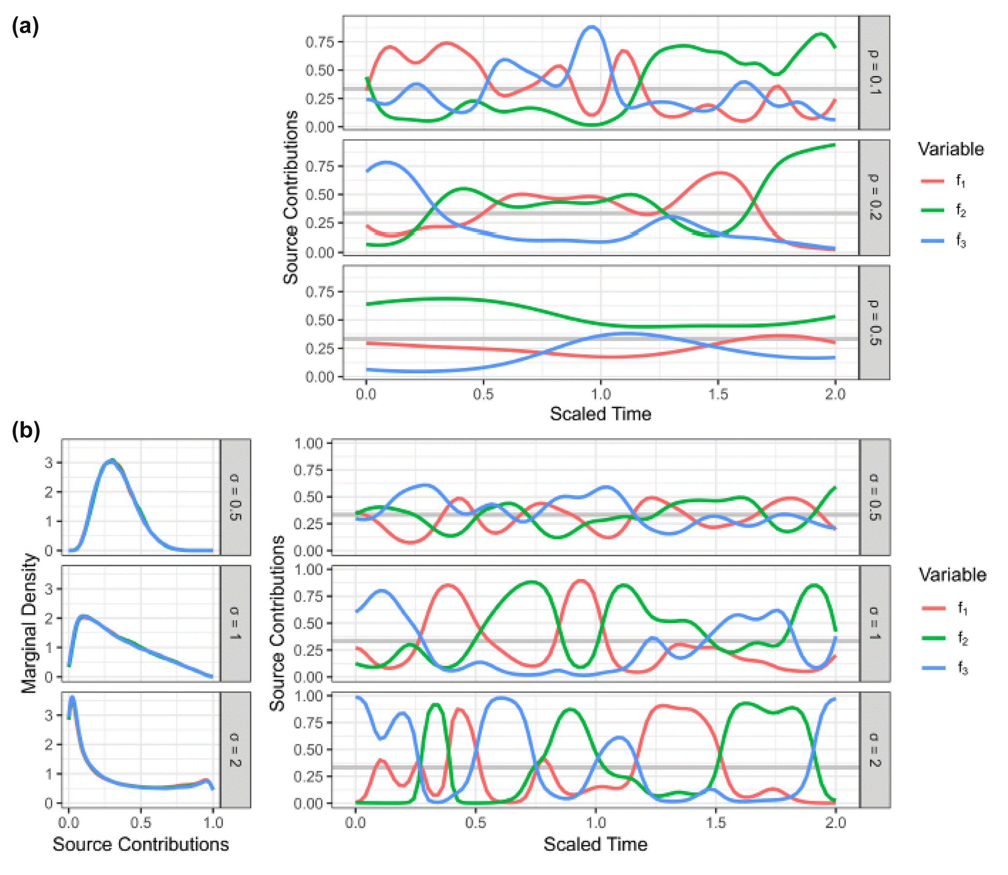
Figure 1Examples of a generalized Gaussian process prior with the radial basis function kernel using different values for correlation length (ρ) and concentration (σ). (a) Prior observation for three sources (f1, f2, f3) mapped to the simplex using the centered log ratio transform, shown over an arbitrary time axis using different values of ρ with σ=1. (b) Estimated marginal densities (left-hand side) of transformed Gaussian process priors for different values of the concentration parameters σ with ρ=0.1, with a prior observation for three sources (f1, f2, f3) shown over an arbitrary time axis on the right-hand side.
2.3.3 Dirichlet–Gaussian process priors
To make use of time series information in the source contributions f and the fraction reacted r, direct priors are desired. These priors can be constructed by sampling auxiliary variables from multiple independent Gaussian processes Z∼𝒢𝒫K(G) and at each point in time inverting the log ratio transformations on the simplex in order to create a time series of simplex-valued variables ft. The fraction reacted rt is constrained to the interval [0,1] and can thus be linked for instance by applying the logit transform logit(r) = at each point in time, which maps it to the entire real axis. Hyperparameters for correlation length and concentration are used to compute the kernel matrix for the Gaussian process. The general shape of these priors is visualized in Fig. 1. Working with the matrix of source contributions and of the fraction reacted , the model can be stated in vectorized form, where the link functions are understood to be columnwise (Fischer, 2023):
Both link functions used can easily be inverted once random variables Z∼𝒢𝒫K(G) and Y∼𝒢𝒫(G) are sampled from Gaussian processes over time . The inverse of the clr transform is given by the softmax function, and the inverse of the logit link is given by the sigmoid function (see Fischer, 2023). The prior on the source contribution parameters G is known as a generalized Gaussian process prior, and techniques such as Taylor expansion can be used to derive analytic approximations (Chan and Dong, 2011). Its marginal is a softmax transformed multivariate Gaussian, which is also known as a logistic normal distribution and serves as an approximation to the Dirichlet distribution (Aitchison and Shen, 1980; Devroye, 1986; Fischer, 2023). Mapping using centered log ratio (clr) transforms thus creates a time series of random variables with approximate Dirichlet marginals, which is referred to as a Dirichlet–Gaussian process (DGP; Chan, 2013).
The marginals are controlled by the parameter σ of the Gaussian process, which now acts as the concentration parameter of the Dirichlet distribution. Since the covariance kernel G is scaled to generate Gaussian random variables with unit variance if σ=1, the marginal distribution in that case is approximately the uniform Dir(1). This can be seen by sampling from the generalized Gaussian process priors and estimating the marginals, as shown in Fig. 1b.
Using the isometric log ratio transform ilr instead of clr reduces the number of Gaussian processes that need to be sampled to K−1 for the source contributions. Inverting this link function is accomplished by applying an orthonormal base transform U to the random variables and then applying the softmax function. Since interpretability of the sampled Gaussian process variables is not required, any orthonormal basis is suitable, and a simple construction using Gram–Schmidt orthogonalization is chosen (Nesrstová et al., 2022; Fischer, 2023):
Shorthand notation is used with correlation length ρ and scale σ included in the kernel computation . Both kernel parameters ρ and σ can be set in advance or given weak hyperpriors. The inverse gamma distribution and the regular gamma distribution are chosen under the assumption that the time variables are scaled appropriately. This hierarchical model benefits especially from the reduced number of Gaussian processes sampled when using the ilr transform, since the kernel covariance matrix must be reconstructed in every sampling step. The number of hyperparameters could be increased by using separate concentrations and correlation lengths for the source contributions F and the fraction remaining r.
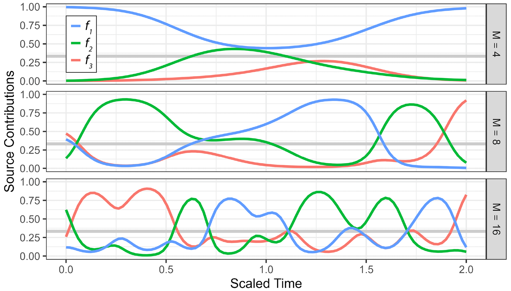
Figure 2Examples of the spline prior for three source contributions (f1, f2, f3, where ) transformed to the simplex with the clr transformation using different degrees of freedom M that can be used to control the covariance of source contributions at separate points in time.
2.3.4 Spline-based priors
An alternative to Gaussian process priors is spline basis functions, which can be used to construct a linear fitting operation that is then mapped to simplex space. This allows for the addition of exogenous variables as predictors of source contributions or fractionation. A cubic spline basis of M basis functions (Fig. 2) is evaluated at the measurement points to form the evaluation matrix with Hij=sj(τi) for polynomial basis functions . The time series of source contributions in simplex space is reconstructed with the basis coefficients bk∈ℝM for each source arranged to the matrix and coefficients for fractionation . This type of model is therefore part of the generalized linear model class (Nelder and Wedderburn, 1972) and allows for easy extension with fixed effects relating to measurement dimensions as well as random effects for experiment replication. It will thus further be referred to as the generalized linear model with spline basis (spline GLM; Fischer, 2023):
In consequence, the distribution of the basis coefficient vector before transformation has distribution for source . After application of the spline basis transform it is thus still Gaussian , although with a modified covariance matrix . Since the inverse centered log ratio transform maps Gaussian random variables with unit variance approximately to a uniform Dirichlet distribution, it makes sense to scale the basis transform such that , as the spline basis vectors are not semi-orthogonal in general.
2.4 Prior distribution for the fraction remaining r
Sampling the prior distribution of the fractionation weight r for closed-system Rayleigh fractionation is challenging, because it is connected through the non-linear logarithm to the effect on measurements. Although a uniform prior usually does not inform the posterior about anything except the boundaries, the effect of the logarithm on the posterior is much more unclear. Different choices for prior distributions of r were thus tested for their effect on the generated posterior sample. The simulated dataset used 17 different values for the fractionation index d ranging from 0.05 to 0.95. Source contributions were fixed to and . Each value of r is used to generate Q=64 data points with measurement error η=4 for a total of 1088 data points (Fig. 4a). The stationary inference model given in Eq. (9) was fitted to each point individually, which makes this setting analogous to the inference procedure used in the original FRAME model (Lewicki et al., 2022).
2.5 Model comparison
2.5.1 Data simulation
No time series datasets with known N2O production and consumption pathway contributions are available; therefore, simulated data must be used for thorough comparison of models. The four models were compared by simulating the data-generating process multiple times and then comparing the resulting posterior sample with fixed truth input values. The time series of source contributions f and pool fractions reacted r used to simulate the data are denoted by and , and the mixing equation with Rayleigh fractionation is used (Eq. 3). Measurement generation is then repeated Q times by sampling the source isotopic signature and fractionation factor ϵ(q)∈ℝd from their respective priors and then adding independent Gaussian measurement errors with noise variance η2∈ℝd for (Fischer, 2023):
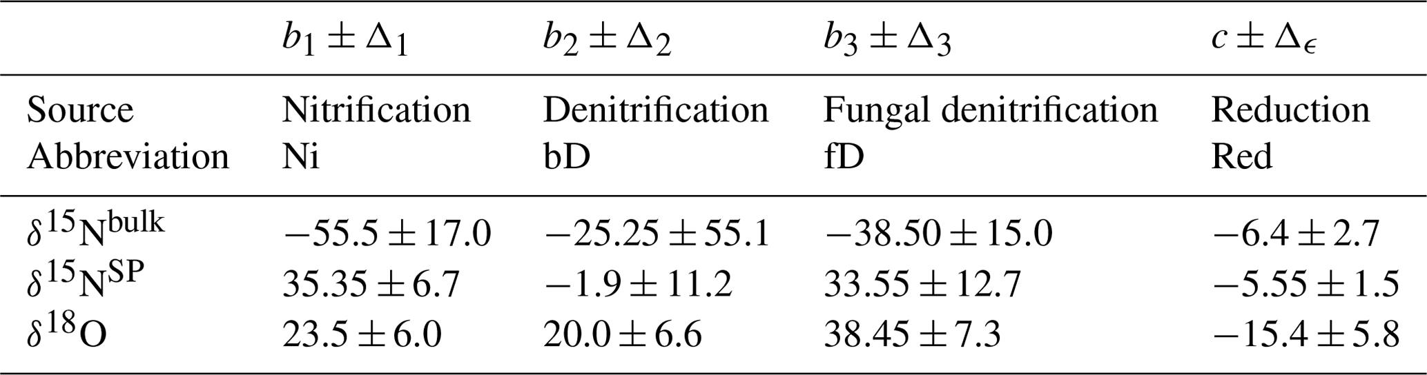
Table 1Prior distribution parameters for N2O source isotopic signatures and the fractionation factor for consumption used to simulate datasets for model testing (Yu et al., 2020). Ranges for sources indicate the full range of previous data used to construct the uniform distribution, whereas for reduction the range indicates the standard deviation of the Gaussian distribution.
Auxiliary data for source isotopic signatures and fractionation factors are taken from Yu et al. (2020) (Table 1). These values correspond to the major N2O sources, nitrification (S1) and bacterial denitrification (S2). Priors are uniform for the sources and Gaussian for the fractionation factor with variance matched to the reported bounds .
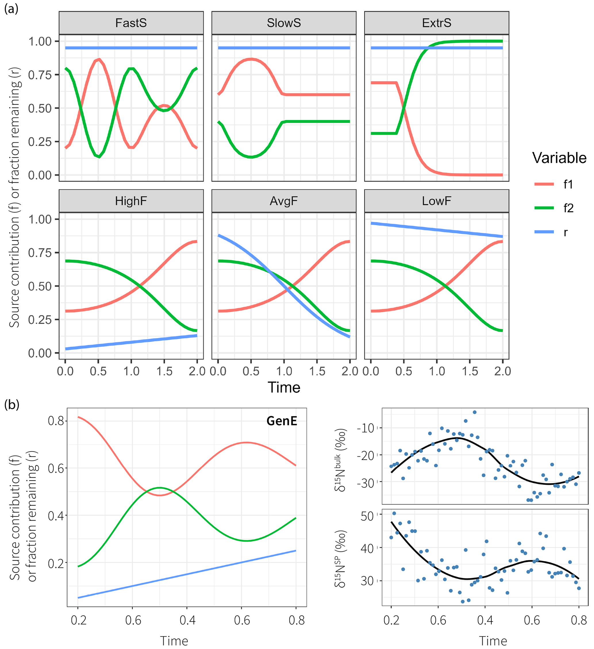
Figure 3True parameter series used to simulate datasets with different properties. The production–consumption scenario corresponds to production by nitrification (S1, red) and denitrification (S2, green) followed by mixing and subsequently reduction (r is the fraction remaining following reduction, blue) in complete denitrification. (a) Six parameter series to test time series modeling, which illustrate fast-changing source contributions (FastS), slow-changing source contributions (SlowS), extremal source contributions (ExtrS), high fractionation (HighF), average and variable fractionation (AvgF), and low fractionation (LowF). (b) The general example (GenE) and the resultant isotopic time series show measurement values simulated accordingly together with LOESS estimates on the right.
The simulations are done on fixed parameter sets that intend to be illustrative for six given cases that might occur in reality. The focus is on investigation of temporal patterns; other fractionation scenarios have been explored previously using a stationary model setup (Lewicka-Szczebak et al., 2020; Lewicki et al., 2022). The true parameter time series and are shown in Figure 3 and are sampled at N=32 equally spaced time steps. One additional general example (GenE) is used for simulation with properties being less extreme than for the other six, which may be more representative of average datasets that would be encountered in practice. For GenE, a Gaussian error with magnitude η=5 is used to sample N=64 measurements . The fixed parameter values and the simulated data are shown in Fig. 3.
Bayesian parameter estimation is then tested on each generated dataset for individually, and a total of S posterior samples of all parameters is produced each time. The posterior samples shall be denoted by and , respectively, for .
2.5.2 Measuring quality of inference
Sampling from the posterior distribution does not give unique point estimates for the parameters involved, and multiple ways of computing final parameter estimates exist. Most commonly the posterior mean is used as point estimate, although using the median could, for example, be a useful strategy for posterior distributions that are highly dissimilar to a Gaussian distribution.
The accuracy of the estimation can be assessed by computing the distance between these pointwise estimates and the true value using root mean squared error (RMSE) and mean average error (MAE). Although it would be possible to compute the metrics at each point in time, they are averaged for simpler model comparison:
Computations for r(q,s) are analogous.
Since the parameters to be estimated are interpreted as a time series, it makes sense to also compare specific time series information across the model estimates. The rate of change can be significantly confounded in the measurement time series, since the measurement errors follow a white noise distribution that introduces high-frequency changes. The ability of models to filter this noise can be measured by comparing the rate of change, which is approximated using first differences: and for . The magnitude of changes is not necessarily relevant, since poor estimates of the magnitude of changes would also lead to poor pointwise comparison metrics. Therefore, the ratio of variances of first differences shall serve as comparison metric for time series information, which can be understood as comparing a notion of curvature or acceleration in the time series (Fischer, 2023):
2.5.3 Metrics for comparison of Bayesian posterior distributions
Bayesian models are mainly used to derive pointwise estimates, but their advantage is the creation of a sample from the posterior distribution. It is thus also important to take distribution properties into account. Posterior interval coverage is a useful metric to evaluate simulated data from the full Bayesian model, meaning in particular that F∗ and r∗ are sampled from their priors as well. Since the data simulation for model comparison used here has fixed parameter values, interpreting interval coverage becomes less meaningful. It is still practical to use the size of the credible interval as measure of uncertainty, and thus the interval span can be compared, which is desired to be as small as possible given otherwise accurate estimates. The credible interval with level is then the set excluding the tails with a proportion of of the most extreme observations on either side (Fischer, 2023):
Further metrics for the quality of the entire posterior distributions can be taken into consideration. Posterior predictive checks are typically used in cases where no true values for the parameter estimates are available, in order to assess the models' capability of representing the input data well (Rubin, 1984). The posterior predictive distribution is the likelihood of hypothetical future measurements calculated using the posterior distribution over parameter values in the presence of the actually available data:
This posterior predictive distribution is not unique due to the auxiliary parameters S and ϵ. It is unclear whether the posterior predictive distribution should be proportional to the marginalized likelihood or rather the likelihood conditioned on the auxiliary parameters . This discrepancy renders comparison of predictive density values across dataset simulations X(q) ineffective, since the models fit a joint posterior and thus assume that future data must be sampled using identical auxiliary parameter values, whereas the simulation resamples their S(q) and ϵ(q) values every time.
The log pointwise predictive density (LPPD) is a metric for the quality of the posterior predictive density and thus by proxy of the Bayesian model. It is computed by evaluating the predictive density at the original data points and can be approximated using the posterior samples (Gelman et al., 2014):
2.6 Model implementation
TimeFRAME is implemented in R R Core Team (2017). Bayesian modeling in TimeFRAME uses Stan for Hamiltonian Monte Carlo sampling (see Sect. 2 in the Supplement). TimeFRAME can be installed using the links provided in the “Code and data availability” section. All experiments were run on an Intel Core i9-10900K CPU. The reported run times in Sect. 2 in the Supplement are for a single sampling chain, and in other sections the reported times are the maximum of four simultaneously run chains.
Table 2Model configurations used to compare performance on time series data across different edge cases for the four model classes described in Sect. 2.3. The “abbreviation” column refers to the abbreviations for each configuration used in subsequent discussion.
In this section, we will first discuss the influence of the prior distribution for r and then present a detailed comparison of different aspects of model performance. The four classes of models were compared for performance on time series data across a wide range of scenarios representative of edge cases that might occur in reality. For these experiments, fixed parameter values for source contributions F∗ and fraction remaining r∗ were sampled as described in Sect. 2.5.1. The model configurations to be compared are summarized in Table 2.
3.1 Influence of the chosen prior distribution for the fraction remaining r
Using a uniform prior for the fraction reacted π(r)∝1 is the natural choice used as standard by all models. This was compared to the Jeffreys prior, which was derived to be and thus is an improper prior (see Sects. 2.2 and Fischer, 2023, for details). A middle ground between these two choices was given by the beta prior , which has . The first argument of the beta distribution can also be used as a free parameter alongside a uniform hyperprior to construct the hierarchical model .
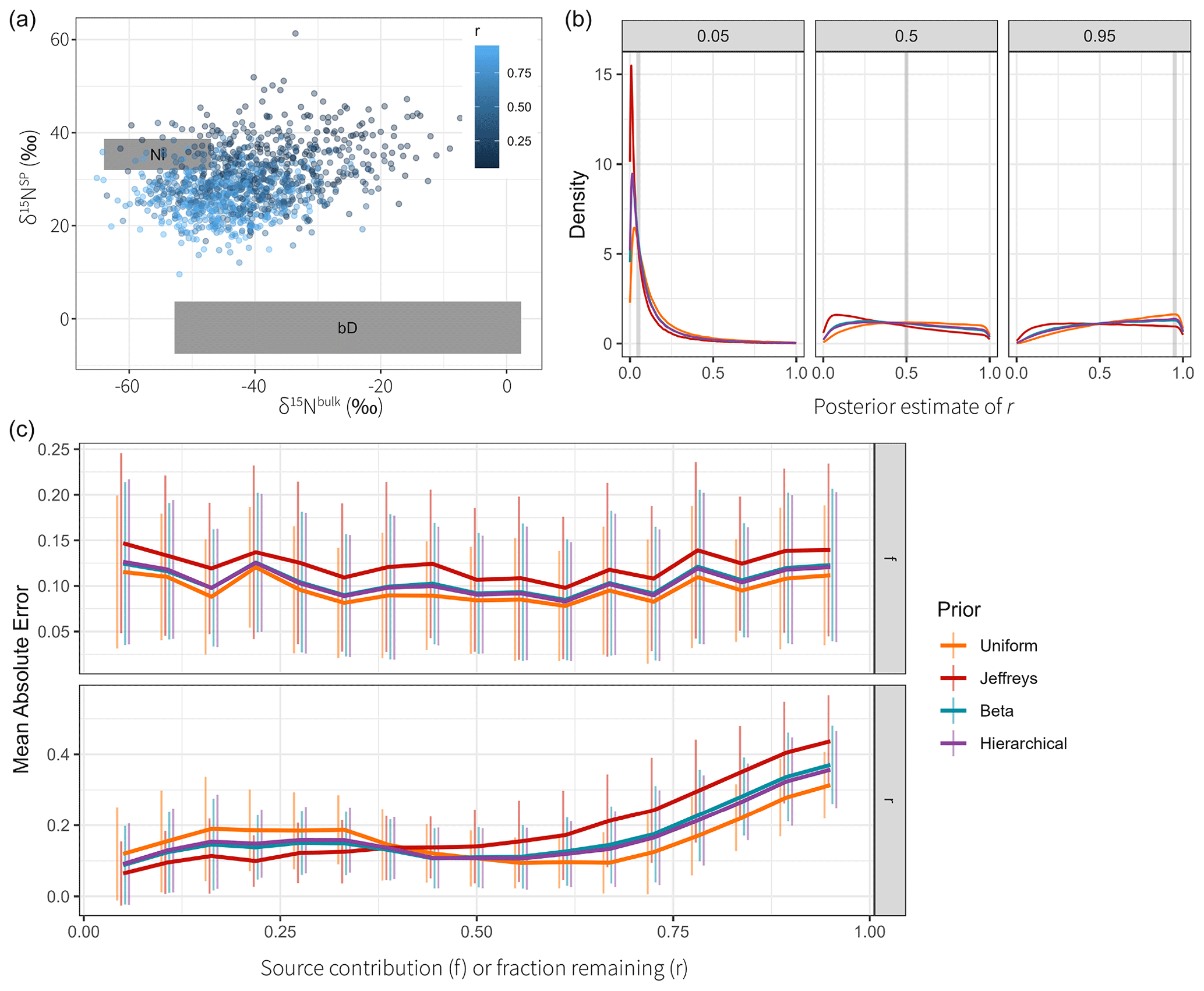
Figure 4Comparison of different priors for the fraction remaining r. (a) Dual-isotope plot for the simulated data, constructed with two sources and different values of r. Data points are colored by the true value of r. (b) Posterior densities of the fractionation weight r averaged across simulations for true r values of 0.05, 0.5, and 0.95 using different prior distributions. (c) Mean absolute error of Bayesian models using different prior distributions of r, shown for different true values of r and f. Vertical lines indicate the standard deviation over Q=64 repetitions. The performance on source contributions is identical for both sources (Ni and bD), since they are perfectly correlated, so only one panel is shown for f.
Each data point was supplied to the model individually, and S=5000 posterior samples were generated. The samples were combined for each value of r to marginalize over the distributions of the auxiliary parameters (Fig. 4b). The source S2 (bD) has a wide prior distribution (Table 1) which confounds with the effect of fractionation and introduces high uncertainty. Since this uncertainty is proportional to the logarithm of r, the effect on the posterior distribution is much more pronounced when r is high. The Jeffreys prior introduces a shift towards lower values compared to the uniform prior, with the beta prior being in between the two. Inference performance was compared by taking the posterior means and and comparing them against the true values (Fig. 4c). Clearly, the Jeffreys prior performs worst for source contributions f, with the uniform prior performing best, closely followed by the beta and hierarchical prior. Regarding the fraction remaining r, the Jeffreys prior performs best for low values of r, with the uniform prior performing worst; however, this relationship switches at about r=0.4 to the opposite. Therefore, choosing any prior can be justified if one expects the fractionation index to be in a certain range. The standard deviation between different repetitions, however, clearly shows that the effect of prior choice is overwhelmed by the variation introduced through the distribution of the sources and consumption, due to the large uncertainty in the source and fractionation factor priors.
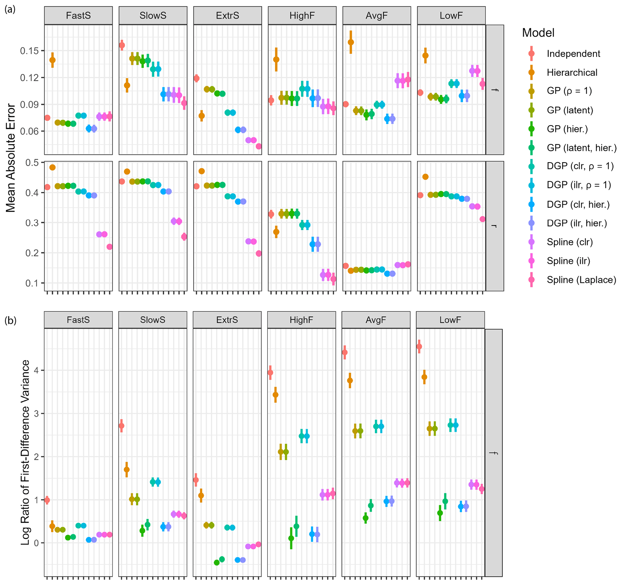
Figure 5Model performance for different configurations (see Table 2 for details: fast-changing source contributions (FastS), slow-changing source contributions (SlowS), extremal source contributions (ExtrS), high fractionation (HighF), average and variable fractionation (AvgF), and low fractionation (LowF)). (a) Mean absolute errors for all examples averaged over Q=64 dataset simulations with standard deviations shown as vertical lines. The results for the two source contributions were identical since they are perfectly correlated, so the plots only show one result for f in addition to the fraction remaining r. (b) Log variance ratio of first differences of the estimated time series against the true values for source contributions f. The time series for fraction remaining r are linear or constant in most examples and are thus not suitable to be used for model comparison with this metric.
3.2 Comparison of overall model performance
The examples described in Sect. 2.5.1 were sampled for Q=64 repetitions. Measurements were simulated with a Gaussian measurement error of magnitude η=5. The posteriors were sampled for a total of S=10 000 steps using four parallel chains. Goodness of estimation was quantified with estimates computed as the posterior means and and taking the mean absolute error (Eq. 21) to the ground truth (Fig. 5a). Conclusions using the root mean squared error or with posterior medians were similar. All models using fixed hyperparameters use default values that are not specifically tuned for the examples at hand. Therefore, the reported performance is not indicative of best-case performance and only shows the quality of the chosen values. Hierarchical models do not have this problem since they can estimate the hyperparameters for each example specifically.
Overall performance was best for hierarchical DGP models and spline GLMs (Fig. 5a). Estimation of fraction reacted r is relatively poor in most cases (MAE > 0.4); however, spline models perform well for all cases (MAE usually < 0.3), particularly for extremal fractionation amounts (all examples except AvgF). The default number of degrees of freedom that spline models use seems surprisingly robust in all examples, whereas the default correlation length of Gaussian processes does not. Gaussian process priors on measurements appear to be slightly worse than DGP priors and spline-based priors, especially SlowS and ExtrS. Independent time step models have worse performance than the rest for all examples, and the hierarchical extension to it only has good performance in examples SlowS and ExtrS, which represent cases where the contribution of the sources is either very low or very high. In other cases, using flat priors as default values seems to work best.
Spline GLMs have very small errors on fraction consumed r whenever the value is slowly changing and close to 0 or 1. This could suggest that the chosen hyperparameters are suitable for all examples. Another plausible explanation is the fact that the spline bases used have an intercept term, which allows the center of estimation to freely move, whereas DGP models do not. For the source contributions this likely does not matter, but allowing the Gaussian process to have non-zero mean could be beneficial for estimating r. An additional spline model was added with Laplace priors on the coefficients, which seems to be beneficial in cases where parameters are close to their boundaries since the prior allows for values farther from zero. The model using Gaussian process priors on measurements was implemented using both formulations with latent variables and with analytically computed likelihood. Performance is identical in all cases, strongly indicating that the formulations are equivalent for parameter estimation. Additionally, using clr or ilr transformations for DGP models and Spline GLMs does not make a difference in estimation accuracy, as is to be expected from their derivations.
Time series models are not only expected to give accurate estimates of mean source contributions and fractionation, but the resulting time series should also have similar properties to the ground truth. The variance ratio of first differences (Eq. 25) measures accuracy of the estimated curvature (Fig. 5b). Clearly, the hierarchical Gaussian process and DGP models estimate the correlation length well, resulting in a time series with similar rates of change to the true values. Spline GLMs perform well, especially for the examples FastS, SlowS, and ExtrS. Independent time step models result in high variation, which is due to the fact that the measurement noise is not adequately filtered. The fixed correlation length Gaussian processes seem to have misspecified hyperparameters, since they also overestimate the rates of change in the time series.
Fitting times ranged from 20 to 72 s on average for the S=10 000 posterior samples generated by each model, split into 2500 over four chains (see Fischer, 2023, for details). Hierarchical models tend to be slowest due to the additional parameters and repeated matrix decompositions that need to be computed, whereas fixed parameter models, especially independent time steps and spline GLMs, are sampled fastest. Spline models using the Laplace prior have long fitting times, which could indicate that the high parameter values – which are allowed due to weaker regularization of parameter ranges far from zero – are not sufficiently identifiable, resulting in slow sample generation.
3.3 Influence of fractionation extent on model performance
Models can have varying performance at different reaction extents and thus different levels of fractionation. For this reason, a time series of source contribution values was taken and paired with different constant fractionation values to generate measurements and monitor performance. In total, 17 equally spaced fractionation values ranging from to 0.98 were used, and a total of Q=32 datasets were generated per value. True values for source contributions were taken from the general example GenE (Sect. 2.5.1), and a measurement error magnitude of η=5 was used. This experiment was done only with representative models of the four main model classes in order to reduce the number of comparisons. The model configurations used were the independent time step model, the Gaussian process prior on measurements with hierarchical estimation of correlation length, DGP prior with hierarchical estimation of correlation length, and spline-based GLM with fixed hyperparameters for degrees of freedom.
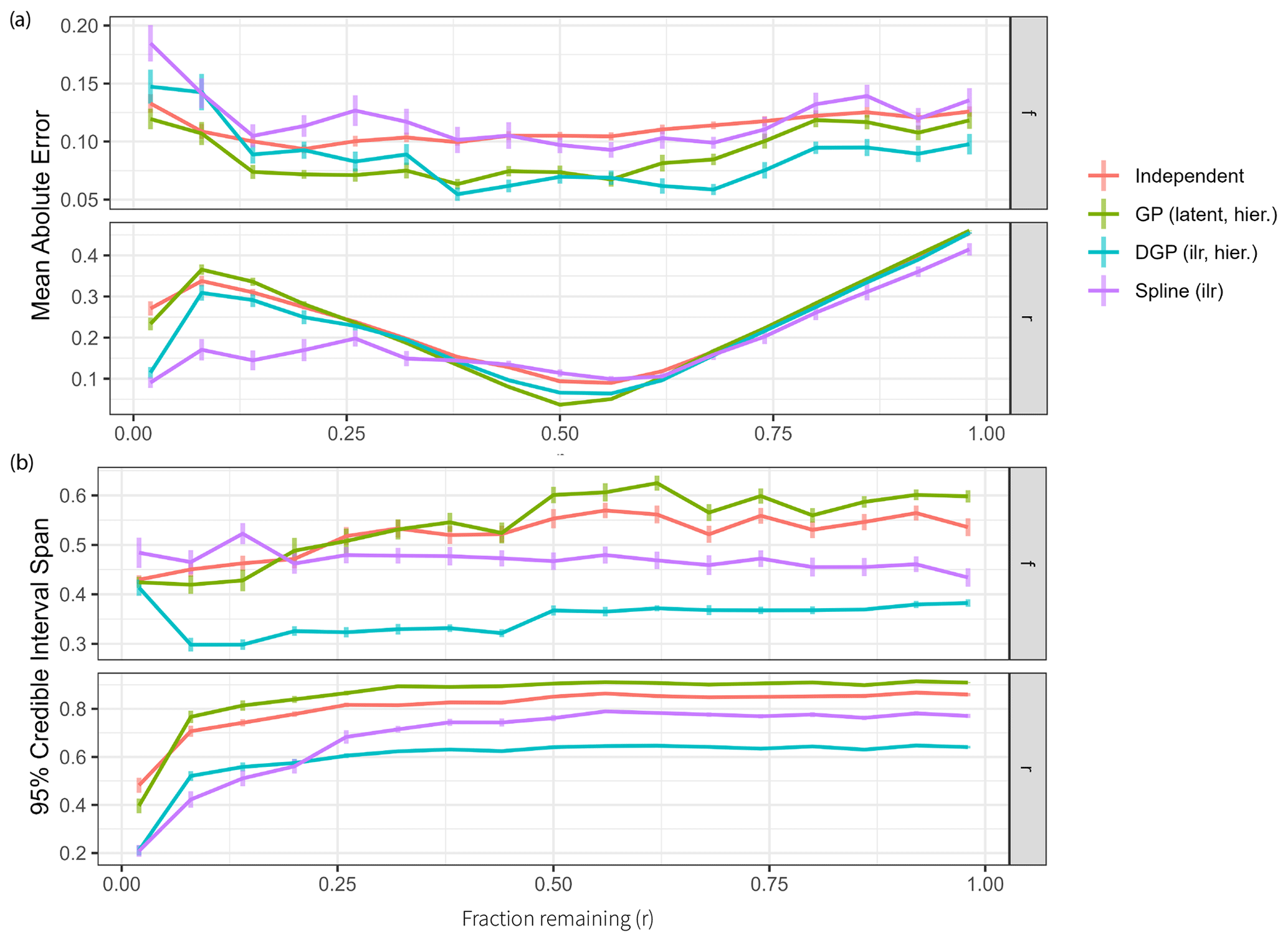
Figure 6Impact of the fraction remaining r on model performance. Each reported value is the average over Q=32 dataset simulations, with vertical lines indicating standard deviations. (a) Mean absolute error of the four main model classes over different values of the fraction remaining r. (b) The 95 % credible interval spans of the four main model classes over different values of the fraction remaining r.
Overall performance is best when r∗ is close to 0.5 (Fig. 6a). Estimation is also more accurate with very low values of r∗, because small r∗ values have large impacts on isotopic measurements, and thus estimation can become more accurate. Spline models are expected to perform well here because the time series of fraction remaining is constant, which can be reflected in the low degrees of freedom used. The different model classes seem to be equally affected by changes in r∗ otherwise, showing that the choice of hyperparameters to reflect the situation of interest is more important than selecting a particular model.
Spans of 95 % credible intervals can give additional insight into the pattern observed for the estimation accuracy over different values of r∗ (Fig. 6b). If parameter estimation is good, then a smaller credible interval span shows a narrow posterior around the correct mean. DGP prior models have the smallest credible interval span for source contributions and fraction remaining. All other models have an interval width of over 0.75 for large values of fraction remaining, thus spanning over half of the possible domain. Clearly, due to the Rayleigh fractionation equation being non-linear in r, it is difficult to estimate large values of r (resulting in low fractionation) with high accuracy. If the amount of remaining substrate is larger than 0.1, the data do not give sufficient information regarding r, so estimates of r group around the prior mean of 0.5 and show large credible interval spans.
3.4 Influence of measurement noise on model performance
The main advantage that smooth models such as Gaussian processes and splines have over the independent time step assumption is that they promise to filter measurement noise and thus produce estimates that are more accurate and have a narrower posterior distribution. For this reason an experiment was conducted using values of source contributions and fraction remaining from the general example GenE (Sect. 2.5.1) to simulate datasets with different levels of measurement noise. Noise values range from η=0.5 to η=20, and for each separate value of η, a total of Q=32 datasets were generated.
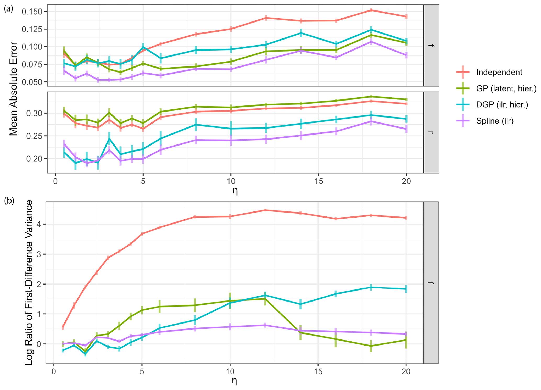
Figure 7Impact of measurement noise on model performance. Each reported value is the average over Q=32 dataset simulations, with vertical lines indicating standard deviations. (a) Mean absolute error of estimation of the four main model classes over different measurement noise levels η. (b) Log variance ratio of first differences for the estimated time series against the true values for source contributions over different measurement noise levels η.
Performance of all models generally decreases with increased measurement noise as expected (Fig. 7a). However, below η=5, reduction in noise does not lead to further improvement in performance: most of the estimation error at this noise level comes from the source end-member uncertainty rather than the measurement noise. The variance ratio of first differences (Fig. 7b) can be used to assess the quality of the estimated time series in the presence of high-frequency changes due to measurement noise. Variance ratios of the independent time series model gradually increase with increasing measurement noise magnitude. All other models seem to filter the noise well, having much lower overestimations of the first difference variance. The hierarchical DGP model seems to be less equipped to deal with very high noise, which could simply be due to the fact that the weakly informative hyperprior on the correlation length is not suitable here. The spline GLM appears to have constant low values for the ratio of first difference variance, due to the fact that the fixed degrees of freedom predetermine the smoothness of the estimates independent of measurement noise. Moreover, the model run time for the spline model was close to the run time for the independent model and less than half the run time for the GP and DGP models across all noise levels. These results show that use of the spline model can be particularly advantageous for data featuring high statistical uncertainty.
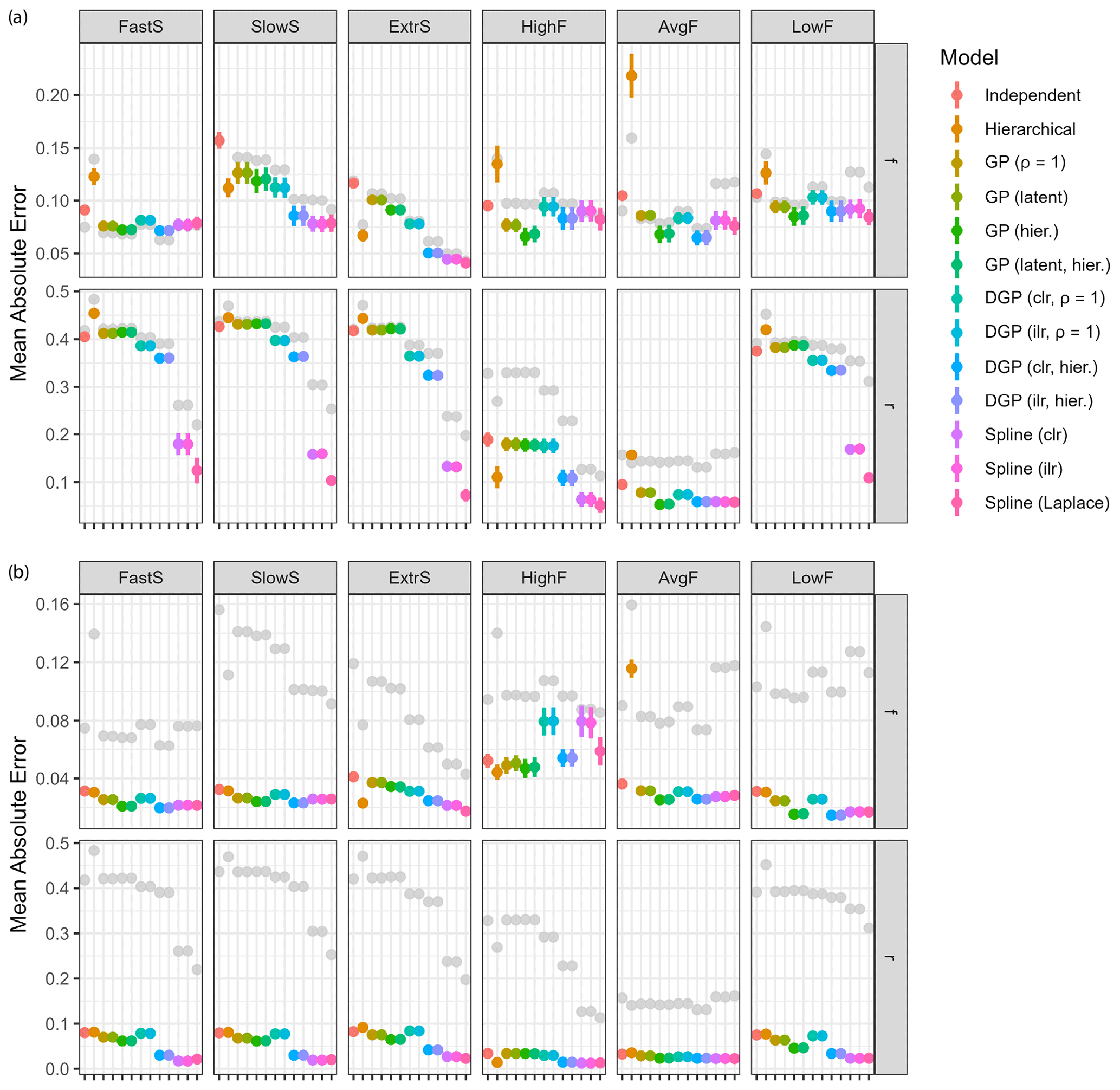
Figure 8Model performance considering different improvements to the input data. The original model performance is shown in gray. (a) Mean absolute error for all models on Q=64 generated datasets using one additional isotopic measurement (δ18O). (b) Mean absolute error for all models on Q=64 generated datasets using the idealized sources and fractionation factor with 10 % uncertainty in isotopic end-members.
3.5 Potential impact of improvements in data quality
Estimation accuracy can be improved not only by choosing the right model but also by improving the quality of the data available to the model. Several ways of adding more or higher-quality data exist, and the effects on model performance were studied in order to find what would be most beneficial. The above examples use two sources with two isotopic measurements, making the system well determined. If additional isotopic measurements are available, they can be added to make the system overdetermined and thus eliminate some noise. To investigate this approach, the additional isotopic measurement δ18O was added with source end-members and uncertainty from Yu et al. (2020) (Table 1). The same dataset generation procedure as in Sect. 3.2 was used with a total of Q=64 datasets generated. Resulting improvement in estimation accuracy for the same two sources is shown in Fig. 8a. It is worth noting that the additional measurement is not ideal in quality, with large uncertainty for the fractionation factor ϵ. An improvement can clearly be seen for estimation of the fraction reacted r, especially in the examples HighF and AvgF. Very little improvement is seen for estimation of f. Spline GLMs improved the most, especially in their already good ability to estimate the fraction reacted. The addition of δ18O to this model did not strongly improve results, due to large uncertainty in source end-members and fractionation factors. However, the addition of isotopic dimensions with low uncertainty or strong differences compared to existing information could improve results, for example, clumped isotopes or δ18O for determination of fungal denitrification.
Instead of adding additional measurements, efforts could be put into determining the end-members of the sources and the fractionation factors more accurately, thus reducing uncertainty in the input data. To study this case an idealized set of sources and fractionation factors were selected to have the mixing and reduction line exactly perpendicular, with an uncertainty of 10 % in each dimension with respect to the mean. This renders the mixing and fractionation components independent, since they cannot confound each other. We therefore set the end-members for S1 to and 1±0.2 ‰ for δ15Nbulk and δ15NSP, respectively, and for S2 to 1±0.2 and ‰ for δ15Nbulk and δ15NSP, respectively. The fractionation factor was set to 1±0.1 ‰ for both isotopes. Measurements sampled in this setting follow exactly the same procedure as in Sect. 3.2 but only use a Gaussian measurement error with magnitude η=0.1. For each example, Q=64 datasets were generated, and the mean absolute error of estimation is shown in Fig. 8b.
Improving all uncertainties involved at a minimum has a great impact on model performance. Almost all mean absolute errors of estimation are below an error margin of 0.05 for source contributions and below 0.1 for fraction remaining. Furthermore, model choice becomes less relevant, and even the independent time step models perform similarly to the other more sophisticated ones. Interestingly, the DGP model with fixed hyperparameters and the spline GLM with fixed spline basis underperform in source contribution estimation, for example, HighF. This could be evidence that the default parameters become less robust when noise is removed, and they should be selected more carefully. This experiment is an extremely idealized case, and natural variability likely precludes this level of precision in end-members for microbial N2O production in soil; however, it shows the high potential for improvements in input data to enhance results and moreover to make results more robust towards model configuration. Currently, the level of uncertainty in direct anthropogenic N2O and CH4 source end-members (e.g., industrial production, energy and transport emissions) is very high due to the scarcity of measurements (Eyer et al., 2016; Röckmann et al., 2016; Harris et al., 2017) – further investigation of the isotopic range of these sources, as well as consideration of end-members for novel isotopes such as clumped species, may lead to the level of uncertainty reduction required to achieve accurate source partitioning.
In this section, we will present use of the TimeFRAME package for the analysis of simulated and real datasets to illustrate aspects of model configuration choice and output data under different scenarios.
4.1 Model selection and application
TimeFRAME allows different models to be applied with minimal effort, meaning that data can be analyzed with several different model setups to investigate the robustness of results. The independent time step model does not incorporate time series information; thus, it is recommended only for datasets with independent measurements. The DGP and spline models both perform well, reproducing the input data values and time series properties – the spline model was better able to estimate r. All models estimate f of different sources across the full range with similar accuracy; however, when the fraction remaining r is very low or high, the results show much larger error (Fig. 8). This is compounded by the difference between mixing followed by reduction (MR) and reduction followed by mixing (RM) models at low values of r (Sect. 1 in the Supplement). We therefore recommend users test both DGP and spline models for time series data and treat results with caution when these models differ strongly. Estimates of very low fraction remaining should also be treated with caution. Despite these points, we find that TimeFRAME offers a strong improvement on previously available methods: accounting for information contained within time series significantly reduces the uncertainty in estimates of f and r, and the package application is simple and fast, as well as easy to document and reproduce.
The testing here focuses on interpretation of N2O isotope data to unravel production and consumption pathways. TimeFRAME can also be applied to other scenarios, for example, trace gases such as CO2 or CH4, or datasets with many more isotopic dimensions through clumped isotope measurements. The number of sources is indefinite as the model can be extended by the user; however, when the number of sources is larger than the number of isotopic dimensions, the model will be poorly constrained. The model can currently only include one consumption pathway applied after mixing – future versions will include more complex setups; however, the uncertainty in input data currently precludes this level of complexity. The examples shown here use time as the dimension of autocorrelation, as time series are the most common kind of data. However, other dimensions could be used, such as temperature in the case of measurements across a gradient of temperature-dependent processes or soil moisture for a set of incubations across a moisture gradient. TimeFRAME's setup allows simple adaptation to different user-defined mixing and fractionation models and fast and reproducible interpretation of these models.
4.2 Application to the general simulated time series
The main purpose of the time series models is to provide estimates of source contribution and fractionation weights with uncertainty. In the sections above, only the performance metrics aggregated over many simulations have been shown. To illustrate the modeling capabilities, the representative general example (GenE) was simulated from fixed parameter values, and the inference results are shown in comparison to the true values.
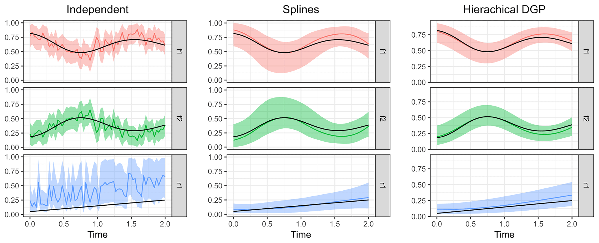
Figure 9Posterior means of the three model types compared to the true parameter values. Shaded areas indicate 95 % credible intervals, and the true parameter values used to simulate the measurements are shown as black lines.
In order to run the Bayesian models and estimate source contributions and fractionation over time, the auxiliary distributions of the source isotopic signatures S and the fractionation factor ϵ as well as the noise magnitude η must be supplied in addition to the dataset. Three different model classes were run to illustrate the computed output: (i) the independent time step model described in Eq. (12), (ii) the spline GLM described in Eq. (18), and (iii) the hierarchical DGP prior model described in Eq. (17). From the output that the models produce, either summary statistics of the posterior (such as its mean and quantiles) can be gathered or the mean and credible intervals from all posterior time series sampled can be extracted as shown in Fig. 9.
The independent time step model clearly shows poorer performance due to the large effect of measurement error on the estimated parameters. Nevertheless, the credible interval covers the true parameter values well and is reasonably narrow. Estimation of the fraction remaining r seems to be biased toward higher values, which could be due to overlap with the variation in source isotopic signatures. The B-spline basis for the GLM seems to have default values for degrees of freedom that are fairly optimal in this case. The time series of parameter estimates is now smooth similarly to the actual parameter series. Estimation using the hierarchical DGP prior model gives the best results: the time series are adequately smooth, and estimates are close to the true values with narrow credible intervals.
4.3 Comparison of TimeFRAME and a dual-isotope mapping approach on a stationary dataset
The samples used to compare the TimeFRAME model with the traditional dual-isotope mapping approach were taken from Kenyan livestock enclosures (bomas in Kiswahili, also known as Swahili) at the Kapiti Research Station and Wildlife Conservancy of the International Livestock Research Institute (ILRI) located in the semi-arid savanna region (1°35.8′–1°40.9′ N, 36°6.4′–37°10.3′ E). The different samples represent the isotopic composition of N2O taken from boma clusters of varying age classes (0–5 years after abandonment). At Kapiti, bomas are set up in clusters of three to four, which are used for the duration of approximately 1 month before setting up a new cluster. The sampling campaign was conducted in October 2021 in order to understand the underlying mechanisms of the huge N2O emissions observed in these systems (Butterbach-Bahl et al., 2020), and the findings will be published in a separate paper (Fang et al., submitted). The dataset contains measurements of δ15Nbulk, δ15NSP, and δ18O of N2O as well as δ15N of soil. A stable isotope analysis of these samples was done using isotope ratio mass spectrometry (IRMS) as described in Verhoeven et al. (2019) and Gallarotti et al. (2021). A dual-isotope mapping approach was used to extract the production pathways and reduction extent for this dataset based on δ15NSP and δ18O using the scenarios of mixing followed by reduction (MR) and reduction followed by mixing (RM), described in detail in Fang et al. (submitted) and Ho et al. (2023).
As the boma dataset is a set of independent measurements, TimeFRAME was applied to the data using the independent time step model. The time axis was replaced by numbering of points in the dataset. The standard deviation of all isotope measurements was set to 1 ‰ as the measurement uncertainty was not quantified; however, this may be a low estimate given the many sources of uncertainty from measurement error to international scale calibration. TimeFRAME was applied in two configurations:
-
using only δ15NSP and δ18O as well as Ni and bD pathways to closely mimic the configuration of the dual-isotope MR approach and
-
using δ15Nbulk, δ15NSP, and δ18O with Ni, bD, and fD (fungal denitrification) pathways, which is the most detailed configuration available with these data.
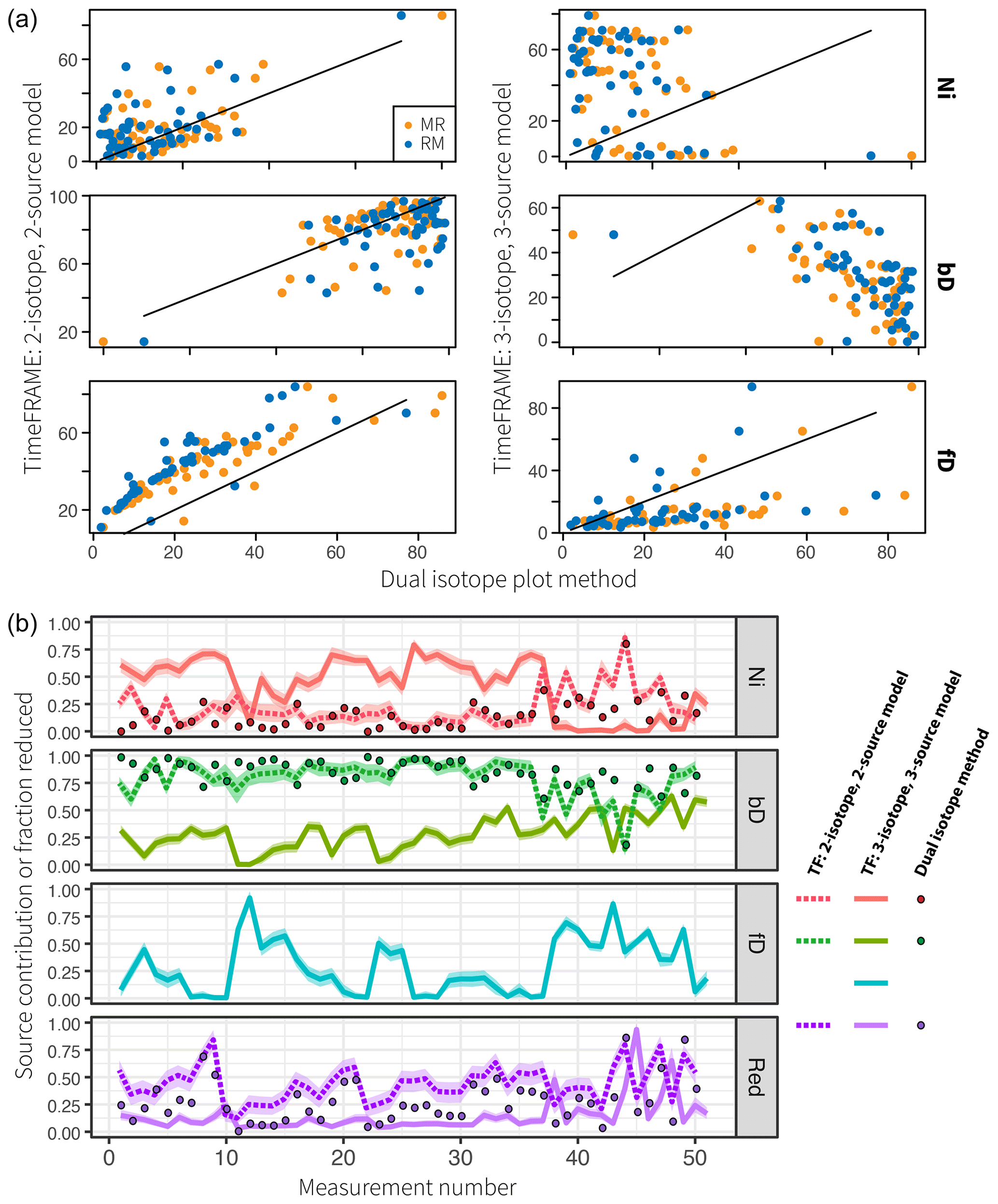
Figure 10Comparison of TimeFRAME results with pathway estimates from a dual-isotope plot approach. TimeFRAME was applied in two configurations: (i) using only δ15NSP and δ18O as well as Ni and bD pathways and (ii) using δ15Nbulk, δ15NSP, and δ18O with Ni, bD, and fD pathways. The dual-isotope approach used δ15NSP and δ18O as well as Ni and bD pathways in configurations MR (mixing followed by reduction) and RM (reduction followed by mixing). (a) A one-to-one comparison of estimates from the two TimeFRAME configurations and the dual-isotope plot MR and RM methods. (b) A plot of the estimates for each pathway from the two TimeFRAME configurations and from the dual-isotope MR method.
The agreement between the dual-isotope method and the analogous TimeFRAME two-isotope implementation is very good (mean absolute deviation of 8 % and 15 % for bD/Ni and reduction, respectively, for the MR method, Fig. 10). The dual-isotope method results are not significantly different for the MR and RM implementations, supporting the assumptions made in Eq. (3) as the basis for the TimeFRAME package: these models only deliver significantly different results in cases where N2O reduction is very high (see Sect. 1 in the Supplement). TimeFRAME offers the major advantage that uncertainty bounds for the prior are incorporated and thus calculated for the posterior. Moreover, using the TimeFRAME package functions, the calculations are reproducible, can be performed in just two lines of code, and can be easily adapted to consider different end-members and model setups. The TimeFRAME three-isotope implementation shows very different results to the other estimates due to the inclusion of δ15Nbulk and the fungal denitrification pathway. This pathway has high δ15NSP (Table 1) and thus strongly impacts the model estimates of nitrification and reduction, which are also evidenced by high δ15NSP.
The pathway estimates were used to reconstruct the isotope measurements, and the RMSE between true measurements and reconstructed measurements was found as an estimate of model performance in the absence of true knowledge of pathways (Table 3). The TimeFRAME two-isotope implementation is able to reproduce the isotopic data more accurately than the dual-isotope plot due to the Bayesian optimization of the fit. The TimeFRAME three-isotope implementation shows poorer RMSE due to the additional challenge of fitting δ15Nbulk as well as the fD pathway. The difference between MR and RM implementations of the dual-isotope approach is minimal, showing that model configuration and uncertainty in end-members is far more important for results than the specific formulation of the fractionation and mixing equation.
Table 3RMSE (‰) for isotopic data estimated using pathway contributions from the two TimeFRAME and the two dual-isotope model configurations, compared to the measured isotopic data used as input for the models.
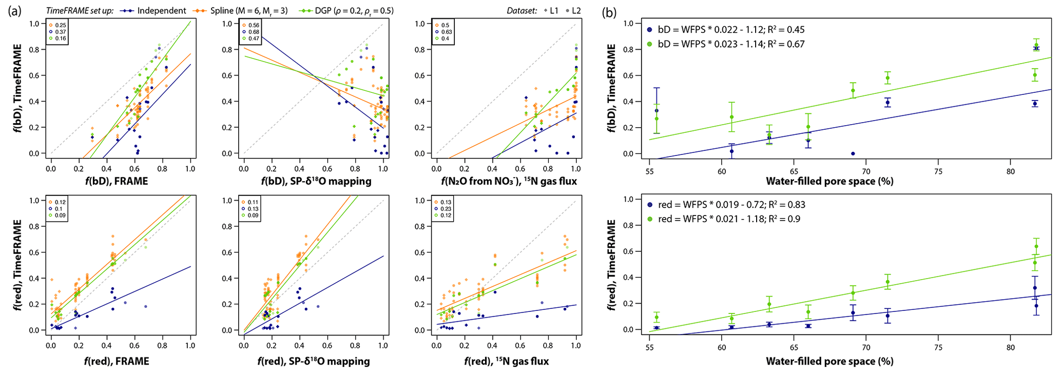
Figure 11Using TimeFRAME to understand the impact of water-filled pore space (WFPS) on N2O production and consumption. (a) Comparison of TimeFRAME pathway estimates (independent, spline (M = 6 and Mr = 3), and DGP (ρ = 0.2 and ρr = 0.5) implementations) with estimates from the FRAME model, from an SP-δ18O mapping approach, and from a 15N-labeled gas flux approach. Comparisons are only shown for bD (bacterial denitrification) and reduction as other pathways are not estimated by the mapping and gas flux approaches. The gas flux approach does not strictly estimate bD but the proportion of N2O arising from substrate. The lines show the linear regression, and the legends show the mean absolute deviation for each comparison. (b) Impact of WFPS on bD and reduction estimated using TimeFRAME spline and DGP results. The error bars show the estimated standard deviation at each point from the TimeFRAME fit. The legend shows details of the weighted linear regression (Rlm() function weighted by ) for each dataset.
These results show the importance of considering different pathways and model configurations. TimeFRAME users should aim to include as much isotopic data as possible and to use other complementary approaches such as microbial ecology to constrain potential production and consumption pathways, for example, to decide whether it is appropriate to include fungal denitrification. Users should consider both the estimated uncertainty for a particular model setup, provided by the TimeFRAME package, and the variation between estimates for different plausible scenarios.
4.4 Comparison of time series analysis with existing approaches
TimeFRAME was applied to two irregularly time-spaced datasets from soil incubations at different soil moisture levels (L1 = drier = 55 %–66 % WFPS; L2 = wetter = 69 %–82 % WFPS). The L1 and L2 incubations were sampled on 8 and 11 dates, respectively, with between 1 and 7 duplicate measurements taken on each sampling date and a total of 41 and 24 measurements made, respectively. The incubations are described in detail in Lewicka-Szczebak et al. (2020). TimeFRAME was compared to results from the 3DIM/FRAME model (Lewicka-Szczebak et al., 2020; Lewicki et al., 2022), with both models considering four pathways (bacterial denitrification, nitrifier denitrification, fungal denitrification, nitrification) as well as N2O reduction using the end-members and fractionation factors reported in Lewicka-Szczebak et al. (2020). FRAME solves the isotopic equations independently for each sampling date, whereas TimeFRAME spline and DGP implementations are able to consider temporal correlations between sampling times. Additionally, dual-isotope mapping and 15N labeling approaches were compared, as described in Lewicka-Szczebak et al. (2020).
The agreement was good between pathway estimates from TimeFRAME and FRAME, although the spline implementation estimated lower reduction than other methods (Fig. 11). Agreement with the mapping approach was very poor for bD and good for reduction, reflecting the low ability of the mapping approach to unravel pathway contributions with similar end-members. Agreement with the 15N gas flux method was good for reduction and acceptable for bD, considering the denitrification contribution being quantified is not identical. The results clearly showed the influence of WFPS on bD and reduction, with both pathways increasing by 2 % for every 1 % increase in WFPS (Fig. 11).
The TimeFRAME data analysis package uses Bayesian hierarchical modeling to estimate production, mixing, and consumption pathways based on isotopic measurements. The package was particularly developed for the analysis of N2O isotopic data and contains default isotopic end-members and fractionation factors for N2O, but the flexible implementation means it can also be applied to other trace gases such as CH4 and CO2. TimeFRAME provides a simple and standardized method for analysis of pathways based on isotopic datasets, which has previously been lacking. The package will contribute strongly to reproducibility and uncertainty quantification in the analysis of these datasets.
TimeFRAME has four main classes of models, which have been extensively tested in a range of scenarios. For time series data, the Dirichlet–Gaussian process and spline GLM priors show very good results. These models are able to smooth time series to reduce the impact of noisy data and deliver good pathway quantification compared to the ground truth for simulated datasets. The independent time step model is strongly impacted by measurement noise but delivers good performance compared to the dual-isotope mapping approach, with simpler and more reproducible implementation as well as uncertainty quantification.
Model application and testing showed that uncertainty in end-members and fractionation factors was the major source of uncertainty in pathway quantification. Reduction of uncertainty in these parameters will strongly improve the insights that can be gained from isotopic data. Model setup is also critical: the sources/pathways chosen in the model strongly affect results and should be informed based on any other relevant sources of information, for example, profiling of the microbial community present at a measurement site. TimeFRAME provides a robust and powerful analysis tool, but the accuracy of results gained from TimeFRAME depends on careful definition of the model setup and configuration by the user.
The TimeFRAME code and application data shown in the paper can be accessed at
The TimeFRAME package for direct installation with devtools is located at
The TimeFRAME user interface (Shiny app) is useful for first interactions with the model. The TimeFRAME shiny app can be directly started at
-
https://renkulab.io/projects/fischphi/n2o-pathway-analysis/sessions/new?autostart=1 (Fischer, 2024).
Alternatively, session settings for the Renku platform deployment can be chosen before the app is initialized at
The development version of TimeFRAME, including the different edge scenarios explored in this paper as well as tools and examples to assist in the implementation of different fractionation equations, can be accessed at
Code used for the experiments can be found at
The supplement related to this article is available online at: https://doi.org/10.5194/bg-21-3641-2024-supplement.
EH and PF wrote the paper with comments and input from other coauthors. PF developed the TimeFRAME package and carried out extensive testing of the tool during his MSc thesis at ETH Zürich under the supervision of EH, FPC, MPL, and DLS. MPL and DLS developed the FRAME package and provided guidance for the expansion to TimeFRAME.
The contact author has declared that none of the authors has any competing interests.
Publisher's note: Copernicus Publications remains neutral with regard to jurisdictional claims made in the text, published maps, institutional affiliations, or any other geographical representation in this paper. While Copernicus Publications makes every effort to include appropriate place names, the final responsibility lies with the authors.
We thank Matti Barthel (Department of Environmental Systems Science, ETH Zürich) for contribution of boma data. Dominika Lewicka-Szczebak was supported by the Polish Returns program of the Polish National Agency for Academic Exchange and the Polish National Science Centre (grant no. 2021/41/B/ST10/01045).
This research has been supported by the Schweizerischer Nationalfonds zur Förderung der Wissenschaftlichen Forschung (SNSF – Swiss National Science Foundation) (grant no. 200021_207348).
This paper was edited by Jack Middelburg and reviewed by two anonymous referees.
Aitchison, J. and Shen, S. M.: Logistic-normal distributions: Some properties and uses, Biometrika, 67, 261–272, https://doi.org/10.2307/2335470, 1980. a
Berger, J. O., Bernardo, J. M., and Sun, D.: Overall Objective Priors, Bayesian Anal., 10, 189–221, https://doi.org/10.1214/14-ba915, 2015. a
Bonnaffé, W., Sheldon, B. C., and Coulson, T.: Neural ordinary differential equations for ecological and evolutionary time-series analysis, Methods Ecol. Evol., 12, 1301–1315, https://doi.org/10.1111/2041-210X.13606, 2021. a
Butterbach-Bahl, K., Gettel, G., Kiese, R., Fuchs, K., Werner, C., Rahimi, J., Barthel, M., and Merbold, L.: Livestock enclosures in drylands of Sub-Saharan Africa are overlooked hotspots of N2O emissions, Nat. Commun., 11, 4644, https://doi.org/10.1038/s41467-020-18359-y, 2020. a
Chan, A. B.: Multivariate generalized gaussian process models, Arxiv [code], https://doi.org/10.48550/ARXIV.1311.0360, 2013. a
Chan, A. B. and Dong, D.: Generalized gaussian process models, in: CVPR 2011, IEEE, Colorado Springs, CO, USA, 20–25 June 2011, https://doi.org/10.1109/cvpr.2011.5995688, 2011. a
Denk, T. R. A., Mohn, J., Decock, C., Lewicka-Szczebak, D., Harris, E., Butterbach-Bahl, K., Kiese, R., and Wolf, B.: The nitrogen cycle: A review of isotope effects and isotope modeling approaches, Soil Biol. Biochem., 105, 121–137, https://doi.org/10.1016/j.soilbio.2016.11.015, 2017. a
Devroye, L.: Methods of Multivariate Analysis, Wiley, ISBN: 978-0-470-17896-6, 1986. a
Eyer, S., Tuzson, B., Popa, M. E., van der Veen, C., Röckmann, T., Rothe, M., Brand, W. A., Fisher, R., Lowry, D., Nisbet, E. G., Brennwald, M. S., Harris, E., Zellweger, C., Emmenegger, L., Fischer, H., and Mohn, J.: Real-time analysis of δ13C- and δD−CH4 in ambient air with laser spectroscopy: method development and first intercomparison results, Atmos. Meas. Tech., 9, 263–280, https://doi.org/10.5194/amt-9-263-2016, 2016. a
Fischer, P.: Using Bayesian Mixing Models to Unravel Isotopic Data and Quantify N2O Production and Consumption Pathways (MSc thesis, ETHZ), MSc thesis, ETH Zurich, https://blogs.ethz.ch/eliza-harris-isotopes/timeframe/ (last access: June 2023), 2023. a, b, c, d, e, f, g, h, i, j, k, l, m, n, o, p, q, r, s, t
Fischer, P.: TimeFRAME: Time-dependent Fractionation and Mixing Evaluation, Contains source files and notebooks for the development of N2O pathway quantification methods, Renku [code], https://renkulab.io/projects/fischphi/n2o-pathway-analysis (last access: 20 November 2023), 2024. a, b, c, d
Gallarotti, N., Barthel, M., Verhoeven, E., Engil Isadora, P. P., Bauters, M., Baumgartner, S., Drake, T. W., Boeckx, P., Mohn, J., Longepierre, M., Kalume Mugula, J., Ahanamungu Makelele, I., Cizungu Ntaboba, L., and Six, J.: In-depth analysis of N2O fluxes in tropical forest soils of the Congo Basin combining isotope and functional gene analysis, ISME J., 25, 3357–3374, https://doi.org/10.1038/s41396-021-01004-x, 2021. a
Gelman, A., Hwang, J., and Vehtari, A.: Understanding predictive information criteria for Bayesian models, Stat. Comput., 24, 997–1016, https://doi.org/10.1007/s11222-013-9416-2, 2014. a
Harris, E. J. and Fischer, P.: TimeFRAME, Gitlab [data set], https://gitlab.renkulab.io/eliza.harris/timeframe (last access: 20 November 2023), 2023a. a
Harris, E. J. and Fischer, P.: TimeFRAME, Github [data set], https://github.com/elizaharris/TimeFRAME, 2023b. a
Harris, E., Henne, S., Hüglin, C., Zellweger, C., Tuzson, B., Ibraim, E., Emmenegger, L., and Mohn, J.: Tracking nitrous oxide emission processes at a suburban site with semicontinuous, in situ measurements of isotopic composition, J. Geophys. Res.-Atmos., 122, 1–21, https://doi.org/10.1002/2016JD025906, 2017. a
Lewicka-Szczebak, D., Augustin, J., Giesemann, A., and Well, R.: Quantifying N2O reduction to N2 based on N2O isotopocules – validation with independent methods (helium incubation and 15N gas flux method), Biogeosciences, 14, 711–732, https://doi.org/10.5194/bg-14-711-2017, 2017. a
Lewicka-Szczebak, D., Lewicki, M. P., and Well, R.: N2O isotope approaches for source partitioning of N2O production and estimation of N2O reduction – validation with the 15N gas-flux method in laboratory and field studies, Biogeosciences, 17, 5513–5537, https://doi.org/10.5194/bg-17-5513-2020, 2020. a, b, c, d, e, f, g, h, i
Lewicki, M. P., Lewicka-Szczebak, D., and Skrzypek, G.: FRAME–Monte Carlo model for evaluation of the stable isotope mixing and fractionation, PLOS ONE, 17, 4–7, https://doi.org/10.1371/journal.pone.0277204, 2022. a, b, c, d, e, f, g
Mariotti, A., Germon, J. C., Hubert, P., Kaiser, P., Letolle, R., Tardieux, A., and Tardieux, P.: Experimental-determination of Nitrogen Kinetic Isotope Fractionation – Some Principles – Illustration For the Denitrification and Nitrification Processes, Plant Soil, 62, 413–430, 1981. a
Nelder, J. and Wedderburn, R.: Generalized linear models, J. R. Stat. Soc. Ser. A-G., 135, 370, https://doi.org/10.2307/2344614, 1972. a
Nesrstová, V., Wilms, I., Palarea-Albaladejo, J., Filzmoser, P., Martín-Fernández, J. A., Friedecký, D., and Hron, K.: Principal Balances of Compositional Data for Regression and Classification using Partial Least Squares, arXiv [stat.ME], arXiv:2211.01686, pp. 1–26, 2022. a
Ostrom, N. E., Pitt, A., Sutka, R., Ostrom, P. H., Grandy, A. S., Huizinga, K. M., and Robertson, G. P.: Isotopologue effects during N2O reduction in soils and in pure cultures of denitrifiers, J. Geophys. Res.-Biogeo., 112, G02005, https://doi.org/10.1029/2006JG000287, 2007. a, b
Parnell, A. C., Phillips, D. L., Bearhop, S., Semmens, B. X., Ward, E. J., Moore, J. W., Jackson, A. L., Grey, J., Kelly, D. J., and Inger, R.: Bayesian stable isotope mixing models, Environmetrics, 24, 387–399, https://doi.org/10.1002/env.2221, 2013. a
Pedersen, K. B. and Petersen, M. S.: The Matrix Cookbook, Technical University of Denmark, http://www2.compute.dtu.dk/pubdb/pubs/3274-full.html (last access: November 2012), 2012. a
R Core Team: R: A anguage and Environment for Statistical Computing, R Foundation for Statistical Computing, Vienna, Austria, 2017. a
Röckmann, T., Eyer, S., van der Veen, C., Popa, M. E., Tuzson, B., Monteil, G., Houweling, S., Harris, E., Brunner, D., Fischer, H., Zazzeri, G., Lowry, D., Nisbet, E. G., Brand, W. A., Necki, J. M., Emmenegger, L., and Mohn, J.: In situ observations of the isotopic composition of methane at the Cabauw tall tower site, Atmos. Chem. Phys., 16, 10469–10487, https://doi.org/10.5194/acp-16-10469-2016, 2016. a
Rohe, L., Anderson, T.-H., Flessa, H., Goeske, A., Lewicka-Szczebak, D., Wrage-Mönnig, N., and Well, R.: Comparing modified substrate-induced respiration with selective inhibition (SIRIN) and N2O isotope approaches to estimate fungal contribution to denitrification in three arable soils under anoxic conditions, Biogeosciences, 18, 4629–4650, https://doi.org/10.5194/bg-18-4629-2021, 2021. a
Rubin, D.: Bayesianly justifiable and relevant frequency calculations for the applied statistician, Ann. Stat., 12, 1151–1172, 1984. a
Stock, B. C., Jackson, A. L., Ward, E. J., Parnell, A. C., Phillips, D. L., and Semmens, B. X.: Analyzing mixing systems using a new generation of Bayesian tracer mixing models, PeerJ, 6, e5096, https://doi.org/10.7717/peerj.5096, 2018. a, b
Verhoeven, E., Barthel, M., Yu, L., Celi, L., Said-Pullicino, D., Sleutel, S., Lewicka-Szczebak, D., Six, J., and Decock, C.: Early season N2O emissions under variable water management in rice systems: source-partitioning emissions using isotope ratios along a depth profile, Biogeosciences, 16, 383–408, https://doi.org/10.5194/bg-16-383-2019, 2019. a
Wolf, B., Merbold, L., Decock, C., Tuzson, B., Harris, E., Six, J., Emmenegger, L., and Mohn, J.: First on-line isotopic characterization of N2O above intensively managed grassland, Biogeosciences, 12, 2517–2531, https://doi.org/10.5194/bg-12-2517-2015, 2015. a
Wu, D., Well, R., Cárdenas, L. M., Fuß, R., Lewicka-Szczebak, D., Köster, J. R., Brüggemann, N., and Bol, R.: Quantifying N2O reduction to N2 during denitrification in soils via isotopic mapping approach: Model evaluation and uncertainty analysis, Environ. Res., 179, https://doi.org/10.1016/j.envres.2019.108806, 2019. a
Yu, L., Harris, E., Lewicka-Szczebak, D., and Mohn, J.: What can we learn from N2O isotope data? Analytics, processes and modelling, Rapid Commun. Mass Sp., 34, e8858, https://doi.org/10.1002/rcm.8858, 2020. a, b, c, d, e, f