Modeling integrated soil fertility management for maize production in Kenya using a Bayesian calibration of the DayCent model

Sustainable intensification schemes such as integrated soil fertility management (ISFM) are a proposed strategy to close yield gaps, increase soil fertility, and achieve food security in sub-Saharan Africa. Biogeochemical models such as DayCent can assess their potential at larger scales, but these models need to be calibrated to new environments and rigorously tested for accuracy. Here, we present a Bayesian calibration of DayCent, using data from four long-term field experiments in Kenya in a leave-one-site-out cross-validation approach. The experimental treatments consisted of the addition of low- to high-quality organic resources, with and without mineral nitrogen fertilizer. We assessed the potential of DayCent to accurately simulate the key elements of sustainable intensification, including (1) yield, (2) the changes in soil organic carbon (SOC), and (3) the greenhouse gas (GHG) balance of CO₂ and N₂O combined.

Compared to the initial parameters, the cross-validation showed improved DayCent simulations of maize grain yield (with the Nash–Sutcliffe model efficiency (EF) increasing from 0.36 to 0.50) and of SOC stock changes (with EF increasing from 0.36 to 0.55). The simulations of maize yield and those of SOC stock changes also improved by site (with site-specific EF ranging between 0.15 and 0.38 for maize yield and between −0.9 and 0.58 for SOC stock changes). The four cross-validation-derived posterior parameter distributions (leaving out one site each) were similar in all but one parameter. Together with the model performance for the different sites in cross-validation, this indicated the robustness of the DayCent model parameterization and its reliability for the conditions in Kenya. While DayCent poorly reproduced daily N₂O emissions (with EF ranging between −0.44 and −0.03 by site), cumulative seasonal N₂O emissions were simulated more accurately (EF ranging between 0.06 and 0.69 by site). The simulated yield-scaled GHG balance was highest in control treatments without N addition (between 0.8 and 1.8 kg CO₂ equivalent per kg grain yield across sites) and was about 30 % to 40 % lower in the treatment that combined the application of mineral N and of manure at a rate of 1.2 t C ha⁻¹ yr⁻¹. In conclusion, our results indicate that DayCent is well suited for estimating the impact of ISFM on maize yield and SOC changes. They also indicate that the trade-off between maize yield and GHG balance is stronger in low-fertility sites and that preventing SOC losses, while difficult to achieve through the addition of external organic resources, is a priority for the sustainable intensification of maize production in Kenya.

1 Introduction

In Kenya, as in many other countries in sub-Saharan Africa (SSA), maize yields have remained low; on average they have been 1.7 t ha⁻¹ compared to the global average of 5.6 t ha⁻¹ over the last decade (2011–2021; FAO, 2023). This contributes to the low self-sufficiency of food production, with around 20 % of the Kenyan population facing severe food insecurity (World-Bank, 2021b). If yields are not improved, increased population growth will further deteriorate food self-sufficiency and food security in general in the coming decades (Zhai et al., 2021), especially considering expected yield declines resulting from more frequent extreme weather events (Lobell et al., 2011). One of the key limitations to sustainable maize production in SSA is the insufficient use of mineral fertilizer and organic inputs (Vanlauwe et al., 2010). Integrated soil fertility management (ISFM) is a sustainable intensification practice that can alleviate these limitations by combining the use of mineral fertilizers with organic inputs (Vanlauwe et al., 2010). Several studies have reported that ISFM has the potential to more than double maize yields in Kenya, especially on infertile soils, due to its positive impact on soil fertility, including soil organic matter (SOM) content (Chivenge et al., 2009, 2011). Furthermore, increasing SOM can help mitigate adverse effects of climate change, offering considerable potential in carbon-depleted soils across SSA (Corbeels et al., 2019). However, the effectiveness of ISFM in increasing yields strongly depends on local site conditions, such as soil and climate (Chivenge et al., 2011).

To close yield gaps in a resource-efficient way and to assess the climate change mitigation potential of ISFM, we need to understand the long-term effects of ISFM practices at a larger scale. Ideally, this would be facilitated by implementing a large number of long-term experiments across a representative range of soil and climatic conditions. However, the significant costs, labor, and time required to maintain long-term experiments limit the number of sites for evaluating the variable effects of ISFM practices under site-specific conditions. In addition, relying on statistical predictive techniques to upscale results from a limited number of sites may lead to low predictive power and large errors because it is unlikely that the effects of soils and climate on yield and SOM would be fully captured in the statistical models.

Biogeochemical process-based ecosystem models, such as DayCent (Parton et al., 1998; Del Grosso et al., 2001), simulate the effects of important driving variables on crop yield and SOM formation using semi-mechanistic functions developed through decades of agronomic and soil research. Because they (partly) embed our current understanding of the complex ecosystem processes, they are more robust for scaling up the yield potential (Saito et al., 2021) and the SOM building capacity (Lee et al., 2020), compared to statistical predictive techniques. However, to avoid bias in model output, it is best practice that models are calibrated and evaluated for local conditions (Necpálová et al., 2015), especially when applied in novel contexts such as different climate zones with different soils.

Although DayCent has been used to estimate SOM stock changes in Kenya on a national scale (Kamoni et al., 2007) and recently to assess the impact of conservation agriculture on SOM in Ethiopia (Lemma et al., 2021), its modules of SOM and maize crop growth have never been rigorously calibrated and evaluated for tropical agroecosystems in SSA. A recent evaluation of DayCent in Kenyan maize systems showed that SOM turnover is underpredicted by the model (Nyawira et al., 2021). Because SOM is coupled to nitrogen (N) mineralization in biogeochemical models, there is the potential that this translates into biased crop responses to N addition and biased crop productivity predictions in any upscaling exercise. A potential solution to this issue is the simultaneous calibration of soil and crop parameters in DayCent using data from local long-term experiments. Ideally, this calibration would include the uncertainty in the model parameters and model outputs (Clifford et al., 2014), so an estimation of uncertainties is possible in upscaling exercises (Stella et al., 2019). This is especially relevant given a recent study showing considerable uncertainty in DayCent's SOM turnover rates, even when calibrated using a range of long-term experiments (Gurung et al., 2020).

In order to use DayCent to assess the potential of ISFM to reduce yield gaps while minimizing environmental impact in Kenya and other SSA countries, this study aimed at using a Bayesian calibration to derive robust DayCent parameters of SOM cycling and maize growth in Kenya. With robust, we mean that the model evaluation statistics are representative of applying the model to new sites with the same climate and soils. We used the experimental data of four long-term ISFM experiments conducted in Kenya over nearly 2 decades (Laub et al., 2023a, b). Of these, two sites were in humid western Kenya and two were in subhumid-to-semiarid central Kenya.

The first objective of our study was to evaluate to what extent DayCent can reproduce the differences in yields and SOM development in response to the addition of different qualities and rates of organic resources combined with different rates of N fertilizer for a number of contrasting sites. The second objective was to evaluate the greenhouse gas (GHG) balance of different addition rates of organic material in ISFM to find the optimal balance between limiting GHG emissions from the soil and optimizing crop yield (that is, sustainable intensification). The reason for this was that ISFM can be a source of N₂O to the atmosphere (Leitner et al., 2020), but compared to standard practices, it reduces soil organic carbon (SOC) losses or even increases SOC (Laub et al., 2023a), thereby mitigating CO₂ emissions.

The specific steps to reach the objectives of this study were (i) to test the capability of an uncalibrated version of DayCent to simulate yield and SOC development of the different ISFM practices; (ii) to calibrate DayCent to represent ISFM under Kenyan conditions using experimental data from four long-term experiments, displaying the uncertainty in model parameters by Bayesian calibration; and (iii) to use the calibrated model to gain understanding of the GHG balance of the different ISFM treatments.

2 Material and methods

2.1 The experimental sites

The present study used data from four long-term field experiments in Kenya, in which the effect of the addition of different organic resources at different rates was tested, either alone or in combination with the application of mineral nitrogen fertilizer, in the context of ISFM. The sites are located in agriculturally important areas in central and western Kenya (Supplement Fig. S1). The Embu and Machanga sites are both located in Embu County, in the central part of Kenya. The Aludeka site is situated in Busia County in western Kenya, while Sidada is located in the adjacent Siaya County, south of Busia (Supplement Table S1). The experiments at Embu and Machanga began in early 2002, while those at Aludeka and Sidada began in early 2005. Therefore, 19 years of data was available in central Kenya and 16 years of data was available in western Kenya (2 sites × 16 years + 2 sites × 19 years = 70 site years = 140 site seasons). The sites cover a range of altitudes, temperatures, and precipitations. Embu, with a mean annual temperature (MAT) of 20 °C and an annual precipitation of 1200 mm, is the coolest site, while Machanga has a MAT of 24 °C and the lowest annual precipitation (800 mm). Sidada (23 °C, 1700 mm) and Aludeka (24 °C, 1700 mm) have a high MAT and receive significantly more precipitation than the sites in central Kenya. There are two rainy seasons at each site, corresponding to two maize growing seasons per year. The long rainy season occurs from March to August or September, while the short rainy season occurs from October until January or February. In terms of soil texture, Machanga and Aludeka have low clay content (13 % clay at both sites), while Sidada and Embu are rich in clay (56 % and 60 %, respectively).

All experiments were set up as a split-plot design with three replicates, with different qualities and quantities of organic resources as main plots and the presence or absence of mineral N fertilizer as subplots. Maize was grown continuously in all experiments, with two crops per year, one in the long rainy season and one in the short rainy season. The experimental design was identical at all four sites and has been described in detail in earlier publications (Chivenge et al., 2009; Gentile et al., 2011; Laub et al., 2023a, b). Organic-resource treatments consisted of high-quality Tithonia diversifolia (TD) green manure, high-quality Calliandra calothyrsus (CC) prunings, low-quality stover of Zea mays (MS), low-quality sawdust from Grevillea robusta trees (SD), locally available farmyard manure (FYM), and a control treatment (CT) without organic-resource additions. Organic resources differed in quality by the contents of N, lignin, and polyphenols (Supplement Table S2). Each organic resource was applied once a year at two rates, 1.2 and 4 t C ha⁻¹ yr⁻¹, while mineral nitrogen fertilizer was applied at a fixed rate of 120 kg N ha⁻¹ (CaNH₄NO₃) in each of the two growing seasons. Of this, 40 kg N ha⁻¹ was applied at planting, and the remaining 80 kg N ha⁻¹ was applied about 6 weeks later. Organic resources were applied only once a year, prior to planting in the long rainy season, i.e., in January or February. They were incorporated to a depth of 15 cm with hand hoes. Furthermore, a blanket application of 60 kg P ha⁻¹ as triple superphosphate and of 60 kg K ha⁻¹ as muriate potash at planting was provided to all plots each season. The plots were kept weed free by hand weeding, two to three times per season, and selective application of pesticides was used when necessary to control armyworm, stem borer, and/or termites.

2.2 The DayCent model

DayCent (2017 version of DD_EVI) is a terrestrial ecosystem model of intermediate complexity (Del Grosso et al., 2001). It simulates daily C and N fluxes within the soil–plant–atmosphere continuum and has been parameterized for several crops and ecosystems (Necpalova et al., 2018). It has submodules to simulate plant growth and organic-resource and soil organic matter (SOM) decomposition, including mineralization of N, soil water and temperature, N gas fluxes, and CH₄ oxidation. The net primary productivity (NPP) of plants is a function of their genetic potential, a simplified phenology, solar radiation, temperature, and stresses such as reduced water or N availability. Here, we used the non-growing degree day version of the DayCent crop module that does not simulate phenology but has a seedling stage with reduced growth until a certain biomass (full canopy) is reached. SOC and soil N in the topsoil are represented by an active, slow, and passive SOM pool, while litter and organic resources are represented by a structural- and metabolic-litter pool (Parton et al., 1987). All SOM pools are conceptual and have no measurable counterparts, whereas the litter pools are semi-quantitative. Their division is based on the measurable ratio of lignin to N in the organic resources and plant litter. DayCent can adequately simulate crop yields, SOC and soil N dynamics, and N₂O emissions in temperate conditions (Del Grosso et al., 2005; Necpálová et al., 2015; Necpalova et al., 2018; Gurung et al., 2020, 2021), but a recent paper showed inadequate performance for tropical conditions (Nyawira et al., 2021).

2.3 Data used for the DayCent model calibration and evaluation

To provide an overall assessment of the performance of DayCent for its use in Kenya, a leave-one-site-out cross-validation approach was applied to evaluate the model performance. Specifically, this involved using a data subset from three of the four sites for model calibration, with evaluation performed using the data from the fourth site. This process was repeated four times, every time with another site serving as the evaluation site. Different data were used for this: maize grain yield and the aboveground biomass, both on a dry matter basis, were available for each cropping season between 2002 and 2020 (further details in Laub et al., 2023b). All these data were used with one exception – the short rainy season of 2019 at Sidada, which had unrealistically high maize grain yields of up to 16 t ha⁻¹. In addition, plot-scale SOC and total N contents in the top 15 cm soil layer were available at several time points and in 2021 for the 0–30 cm soil depth. At Embu and Machanga, soil samples were taken every 2 to 3 years since the start of the experiment in 2002 until 2021, while at Sidada and Aludeka, soil sampling occurred only in 2005, 2018, 2019 and 2021 (further details in Laub et al., 2023a). Because soil bulk density data were not available for most time points and there was no significant difference in topsoil bulk density between treatments at any site in 2021, the mean soil bulk density per site was used to calculate SOC stocks of the top 15 cm of soil depth. We used a DayCent parameterization that was developed to simulate SOC stocks of the IPCC-recommended (Intergovernmental Panel on Climate Change) 0–30 cm topsoil layer (Gurung et al., 2020) (further details in Sect. 2.3.2). Thus, the 0–15 cm SOC stocks were adjusted to 0–30 cm depth. This was done by adding the site-specific SOC stocks from the 15–30 cm layer (specifically, the 15–30 cm equivalent soil-mass-based ones; Wendt and Hauser, 2013; Lee et al., 2009) to the treatment-specific SOC stocks from 0–15 cm. Due to limited data availability for the 15–30 cm soil depth (only 2021), this approach was considered the most conservative and robust; subsoil carbon usually changes very slowly, and a statistical test revealed no differences in the equivalent soil-mass-based SOC stocks of the 15–30 cm layer (2.5–4.7 t soil ha⁻¹) between treatments at the same site in 2021 (with only one single exception at Aludeka; Supplement Fig. S2).

Data on N₂O emissions were used in the model evaluation phase but not for model calibration, due to their scarcity and high uncertainty. The N₂O measurements were conducted after N fertilization in 2005 (weekly measurements from March to June at Embu and Machanga and daily measurements at Machanga in November), in 2013 and 2018 (weekly measurements from March to the beginning of May at Sidada and Aludeka), and in 2021 (weekly measurements from mid-March to mid-May at Sidada). The measurements applied the static-chamber method (Hutchinson and Mosier, 1981) with two measuring frames per plot permanently installed for a whole rainy season (one within, one between maize rows). The sampling chambers (0.27 × 0.375 × 0.11 m) had a vent tube and fan for homogenizing the gas sample before extraction with a 60 mL polypropylene syringe through a septum-sealed sampling port. Four gas samples were collected at 0, 15, 30, and 45 min of chamber closure. Gas samples from within and between maize rows were combined per time point in the same syringe (Arias-Navarro et al., 2017). All analyses were conducted using an SRI 8610C gas chromatographer (456-GC, Scion Instruments, Livingston, United Kingdom) equipped with an electron capture detector for N₂O analysis. Fluxes per surface area were determined using the linear slope of gas concentration over time (Pelster et al., 2017; Barthel et al., 2022). Simulated N₂O emissions were evaluated against measured daily and cumulative N₂O emissions. To determine the cumulative emissions at the plot scale, we used the trapezoid method (Levy et al., 2017), specifically, the trapz function of R (Tuszynski, 2021). Treatment-scale means and variances of the daily and cumulative N₂O emissions were then computed in a similar way as for the other measurements.

Finally, continuous soil moisture measurements were conducted using sensors placed in each replicate at 10 cm soil depth (EC-5 Soil Moisture Sensor, METER, Germany) in the control and the 1.2 t C plots of the Calliandra, farmyard manure, and maize stover treatments at the Sidada and Aludeka sites (March 2018 to December 2020). These soil moisture data were used to initially determine the optimal pedotransfer functions for soil hydraulic conductivity but not used in the model calibration.

2.3.1 Model driving variables and model assumptions

The site-specific crop management data were obtained from season- and site-specific records of field management operations. These included dates of organic-resource application, manual plowing before planting, maize planting, split application of mineral N, weeding, and harvest. Dates of pesticide applications and gap filling or maize thinning were also available, but these operations are not part of standard DayCent management and were therefore not included in modeling. Therefore, our model runs assumed no occurrence of pests or diseases and an optimal plant density at emergence, which, in practice, was ensured by manual thinning and gap filling.

Recorded weather data existed for all sites, but filling in data gaps was necessary due to the unavailability and loss of recorded data. At Embu and Machanga, manual recordings of daily minimum and maximum temperature and precipitation were available from 2002 until the end of 2007, but from 2008 until 2017, only measured precipitation was available. After 2017, newly installed TAHMO stations (https://tahmo.org/climate-data/, last access: 16 May 2022) were available for these two sites, providing daily values for temperature and precipitation. At Aludeka and Sidada, manual recordings of daily minimum and maximum temperature and precipitation were available for all years from 2005 to 2017. Thereafter, weather stations (METER climate station, METER Environment, Munich, Germany) were installed and provided the data. Data gaps were filled using the NASA POWER product (https://power.larc.nasa.gov/docs/methodology/, last access: 19 May 2022). A bias correction for the minimum and maximum temperature of NASA POWER data was performed, using a linear regression with measured data as the dependent variable (y) and NASA POWER data as the independent variable (x). Specifically, the slope and intercept of the regression equation $y=mx+b$ were used to produce a corrected estimate of these data. In our specific case, the slopes were not significantly different from 1, but intercepts (b) were significantly different from 0. The specific intercepts for the maximum temperature were −0.3, −0.4, +3, and +6 °C for Embu, Machanga, Sidada, and Aludeka, respectively. The intercepts for the minimum temperature were −0.25, −0.5, −3, and +1 °C for Embu, Machanga, Sidada, and Aludeka, respectively. For precipitation, no bias correction was done.

The data on the soil hydraulic properties needed in DayCent (volumetric soil water content at field capacity, wilting point, and saturated hydraulic conductivity K_S) were calculated based on the soil texture measured at each site. The pedotransfer functions of Hodnett and Tomasella (2002) were used because they were specifically designed for tropical soils. Their soil hydraulic properties also showed better agreement between the measured and simulated soil moisture contents than when soil hydraulic properties of Saxton and Rawls (2006) were used. Because the Hodnett and Tomasella (2002) equation does not provide a method to estimate K_S, K_S was calculated using the Saxton and Rawls (2006) equation, with values of the water retention curve, α and n (van Genuchten, 1982), calculated with the equation from Hodnett and Tomasella (2002). The equations can be found in Supplement Sect. S1.

2.3.2 Initial model parameterization and selection of potentially sensitive parameters for calibration

It was assumed that the organic-resource inputs had the same properties across all sites (i.e., mean values of lignin contents and $\mathrm{C}/\mathrm{N}$ ratios per organic resource were assumed; Supplement Table S2). This approach was used because measurements were not available for all sites and years and was justified as an analysis of variance of data from the years 2002, 2003, 2004, 2005, and 2006 at Embu and Machanga, as well as from 2018 at all sites, did not indicate any significant differences in lignin contents and $\mathrm{C}/\mathrm{N}$ ratios between the sites or years. The C content of maize grain was assumed to be 42.5 % throughout the simulation period. This was the mean value of measured grain C content across sites (standard deviation of 1.8 %) in the short rainy season 2018 and long rainy season 2019 (data not shown). Given the strong correlation between maize grain yield and aboveground biomass in the measured data (r=0.87), the aboveground biomass data were transformed to harvest index data for the model calibration process because harvest index had a lower correlation with yield (r=0.59) than aboveground biomass.

The DayCent simulations were conducted at the treatment scale using average values across all three replicate plots for soil parameters (i.e., soil texture, bulk density, pH), SOC and soil N stocks, maize grain yield, and aboveground biomass/harvest index. This aggregation was done to reduce the computation time of the simulations and because initial tests showed similar model performance as compared to applying the model to each experimental replicate individually. The site-specific standard deviation for each type of measurement was used as a measure of uncertainty in the measured data (computed from the three replicates at each time point for each treatment at each site). This choice was based on the statistical models of Laub et al. (2023a, b), showing variance heterogeneity between sites but not between treatments.

The standard parameter values of the DayCent 2020 version were taken as initial model parameters, with three exceptions. First, we used the adjusted decomposition parameter values of the SOM pools from Gurung et al. (2020) to allow for the use of DayCent for simulating SOC stocks of the 0–30 cm soil depth layer instead of the standard 0–20 cm layer. Second, we modified the parameter value representing the fraction lost as CO₂ upon structural-litter and lignin turnover (ps1co(1&2)&rsplig). The default value for this parameter is 0.5, assigning a carbon use efficiency (CUE) value of 50 % to structural litter, based on outdated theories that lignin-rich materials form stable SOC most efficiently (Frimmel and Christman, 1988). Newer studies have, however, clearly shown that minimal structural litter is conserved in the long term, while metabolic litter forms SOC more efficiently (Cotrufo et al., 2013; Denef et al., 2009; Puttaso et al., 2013; Kallenbach et al., 2016). Thus, we opted for a more realistic prior value of 0.85 for ps1co(1&2)&rsplig, corresponding to a more plausible CUE value of 15 % for structural litter (Mueller et al., 1997). Third, for the parameters determining the minimum and maximum proportion of nitrified N lost as N₂O, we used values that fell between the DayCent default values and recent values from Gurung et al. (2021). This choice was motivated by the fact that the DayCent default parameter values led to excessively high emissions, while the Gurung et al. (2021) parameter values resulted in emissions that were too low. Finally, we assumed that the maize growth parameters of the second highest production level (C5 in DayCent) represent best the production levels observed in the experiment.

To identify which model parameters to include in the global sensitivity analysis (see Sect. 2.4) and model calibration, we reviewed the literature for recently conducted sensitivity analyzes of the DayCent model (Necpálová et al., 2015; Gurung et al., 2020). Additionally, we consulted the DayCent manual to identify and add further parameters of potential importance for the processes considered in our study (i.e., plant productivity and soil C and N cycling). This resulted in a selection of 66 parameters (Table 1 and Supplement Table S3). Some of these parameters belong to the same category but can be individually calibrated in DayCent. For example, the “tillage multiplier” of SOM turnover can have different values for different SOM pools but is usually the same for all SOM pools in the standard DayCent parameterization. Thus, we decided to have the same tillage multiplier value for all SOM and litter pools. Some parameters can have different values between the surface and soil SOM pools (e.g., $\mathrm{C}/\mathrm{N}$ ratios and turnover rates). For simplicity, we assigned the same $\mathrm{C}/\mathrm{N}$ ratios and a constant ratio to the turnover rates of surface and soil SOM pools (i.e., decX(2)/decX(1), with X being a number between 1 and 5, representing each of the five defined SOM pools). This simplified parameter sensitivity analysis and calibration with regard to surface and soil SOM pools. Finally, the parameters governing the minimum and maximum values were reformulated. Instead of calibrating them as a maximum and a minimum value, we considered the maximum value and the difference between the minimum and maximum values (i.e., N2Oadjust_(max−min) and aneref(1)−aneref(2)). This ensured that the minimum value was smaller than the maximum value, thereby avoiding numerical problems (initial N2Oadjust_max was set to 0.015; N2Oadjust_(max−min) was set to 0.003).

2.3.3 Soil organic matter pool initialization based on measured data

Instead of relying on spin-up simulation based on uncertain historical land use and management of the simulated sites, we used measured mineral-associated organic carbon (MAOC) fractions as a proxy for the initialization of the passive SOM pool (Zimmermann et al., 2007). Replacing SOM initialization assumptions with measured proxies can enhance model performance (Laub et al., 2020; Wang et al., 2023) and, more importantly, is less sensitive to user assumptions. It also aligns with the DayCent concepts on SOM; the manual (Hartman et al., 2020) denotes that particulate organic carbon (POC) and MAOC are related to the slow and the passive SOM pool, respectively. MAOC data for samples from the 0–30 cm soil layer were available from the year 2021 (specifically for the control −N, control +N, and the farmyard manure −N and Tithonia diversifolia −N treatments at 4 t C ha⁻¹ yr⁻¹ at all sites). It was derived by density fractionation using a sodium polytungstate solution (1.6 g cm⁻³ for Aludeka and 1.7 g cm⁻³ for the other sites). Aggregates were dispersed with ultrasonication at 400 J mL⁻¹ (217 s at 200–240 W), after which samples were centrifuged for 2 h at 4700 rpm to separate the heavy and the light fraction, which were then separated, washed with deionized water, dried at 60 °C for 24 h, and analyzed for weight and C content. A statistical analysis revealed the absence of treatment differences within the same site, so the site-specific MAOC values for the 0–30 cm soil depth across treatments (0.91, 0.88, 0.85, and 0.86 g MAOC g⁻¹ SOC for Aludeka, Embu, Machanga, and Sidada in 0–30 cm, respectively) were used to initialize the SOC in the passive SOM pool in DayCent simulations. Further, 3 % of initial SOC was assigned to the active SOM pool (mean value recommended in the DayCent manual), and the remainder of SOC was assigned to the slow SOM pool.

The DayCent manual further states that, although the slow SOM pool is closely related to the POC fraction, it tends to be larger (Hartman et al., 2020). Consequently, the passive SOM pool must be smaller than the MAOC fraction. Additionally, the fractionation data were from 2021, when the experiments were already 19 and 16 years old. To address these issues, two new parameters were introduced in the simulations: (1) an intercept (IC_MAOC) to account for the passive SOM pool being smaller than the MAOC fraction and (2) a slope for the time since the start of the experiment (SL_t) to account for SOM changes (mostly losses) since the start of the experiments, with the passive SOM pool typically changing at the slowest rate. Given that all sites were converted to agriculture only a few decades ago (Laub et al., 2023a), the percentage of total C in the passive SOM pool at the start of the experiment should be higher than the 30 %–40 % that is common at the steady state of SOM pools (Hartman et al., 2020). Considering this, it was assumed that the intercept's initial value was −0.1 g MAOC g⁻¹ SOC and the slope's initial value was −0.005 g MAOC g⁻¹ SOC yr⁻¹ since the start of the experiment, giving both terms approximately the same weight. Thus, the fraction of SOC in the passive SOM pool at the start of the experiment was

$$\begin{array}{}\text{(1)}& {\mathrm{SOC}}_{\mathrm{p}}\left(\mathrm{g}{\mathrm{g}}^{-\mathrm{1}}\right)={\mathrm{MAOC}}_{\mathrm{2021}}+{\mathrm{IC}}_{\mathrm{MAOC}}+{\mathrm{SL}}_{\mathrm{t}}\times t_{\mathrm{dif}}.\end{array}$$

Here, SOC_p represents the fraction of SOC in the passive SOM pool at the start of the experiment, MAOC₂₀₂₁ is the MAOC fraction in 2021 (g MAOC g⁻¹ SOC), IC_MAOC is the intercept, and SL_t is the slope value that is multiplied by the time difference between the measurement and the start of the experiment in years (t_dif). With the selected standard values for IC_MAOC and SL_t, between 66 % (Machanga) and 73 % (Aludeka) of SOC were assumed to be in the passive SOM pool at the start of the experiment. The uncertainty related to this initialization approach was accounted for in the model calibration by allowing large ranges for these parameters. Finally, to initialize the soil N pools, $\mathrm{C}/\mathrm{N}$ ratios of the active, slow, and passive SOM pools were set to 10, 17.5, and 8.5, respectively, which are the best estimates provided by the manual (Hartman et al., 2020).

2.4 Global sensitivity analysis

To reduce the number of optimized parameters during the calibration, we performed a parameter screening (van Oijen, 2020). For this purpose, a global sensitivity analysis was conducted to quantify the relative importance of different model parameters to the relevant model outputs regarding our study's focus on maize yield and the greenhouse gas mitigation potential of ISFM. The aim was to identify and fix less influential model parameters to their initial values, reducing the computational cost for performing the consecutive Bayesian model calibration (see Sect. 2.5). The global sensitivity analysis was performed using the Sobol method (Saltelli, 2002a, b), which allows for the estimation of the proportion of variance in the model outputs that is explained by each model parameter while considering the first-order and higher-order interaction terms (Gurung et al., 2020). The “sensitivity” package (function sobolSalt; Iooss et al., 2021) of R version 4.0 (R Core Team, 2020) was applied. This function implements a simultaneous Monte Carlo estimation of first-order and total-effect Sobol indices. The computational cost is N(p+2) model runs, with N being the dimension of the two matrices to construct the Sobol sequence and p being the number of parameters (66 in our case). Our tests indicated similar results for N=500 and 1000, so we chose a dimension of 1000. The preselected model parameters to include are described above and in Table 1 and Supplement Table S3. The ranges used for the global sensitivity analysis were centered around the initial parameter value obtained as described above (Sect. 2.3.2). The upper and lower parameter boundaries were based on previous sensitivity analyses (e.g., Necpálová et al., 2015; Gurung et al., 2020), with plausible ranges reported in the DayCent manual and variations observed in different maize parameterizations in the literature. The parameters were then grouped according to the magnitude of their ranges. Parameters with very small, small, and moderate ranges were varied by ± 10 %, 25 %, and 50 % from the initial parameter value, respectively. For parameters with large and very large ranges, the upper boundaries were the initial parameter values multiplied by 3 and 10, respectively, and the lower boundaries were the initial parameter values divided by 3 and 10, respectively. The parameter sensitivity was independently determined for the mean maize grain yield and aboveground biomass, averaged over all seasons at all sites, as well as for the SOC and soil N stocks at the end of the simulation period (equations presented in the Supplement Sect. S2).

Table 1 DayCent model parameters and the coefficient of variation used in the calibration. Displayed are parameters considered for calibration due to a total sensitivity index >2.5 % (top) and with a total sensitivity index >1 % (bottom). The remainder of parameters (<1 %) are not included in this table and can be found in Supplement Table S3. The presented calibrated parameter values correspond to the single parameter set with the highest likelihood, which was derived using the data from all four sites combined. The posterior was also derived using the data from all four sites combined. CV: coefficient of variation, SD: standard deviation, 95 % CI: 95 % credibility interval, Ly: langley (1 Ly = 41 840 J m⁻²).

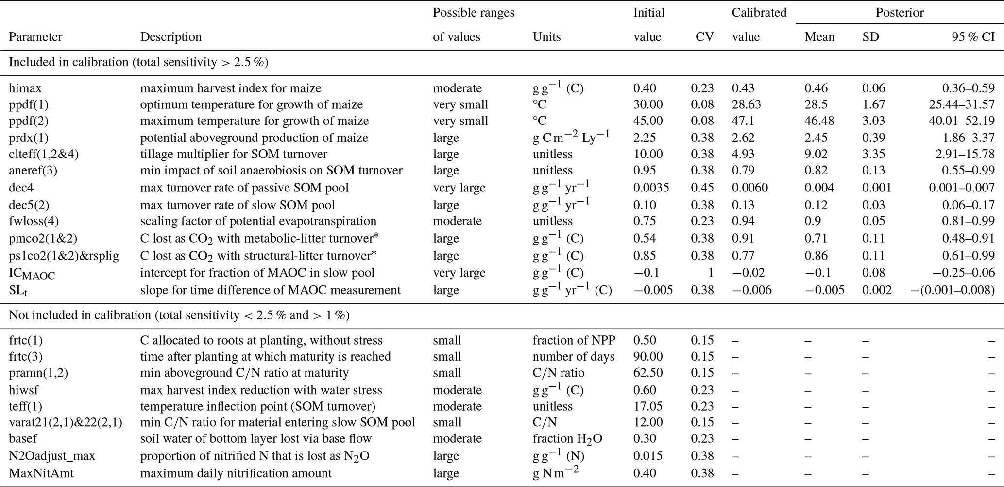
^* 1 − microbial carbon use efficiency.

2.5 Combined Bayesian calibration of plant and soil model parameters

Bayesian calibration is a probabilistic inverse modeling or data assimilation technique, which is used to estimate the joint posterior distribution of model parameters (θ) given the measured data (D) and the model structure (M), expressed as p(θ|D,M). It uses the proportionality form of Bayes' theorem, where p(θ|D,M) is proportional to the prior belief about model parameters, with p(θ) times the likelihood function of the data given the model and the parameters of p(D|M,θ):

$$\begin{array}{}\text{(2)}& p(\mathit{\theta }\mathrm{|}\mathit{D},\mathit{M})\propto p\left(\mathit{\theta }\right)\times p(\mathit{D}\mathrm{|}\mathit{M},\mathit{\theta }).\end{array}$$

While the prior p(θ) is chosen based on previous knowledge of the model parameters, the likelihood function p(D|M,θ) measures how well the model and the data match. In practice it is derived for a given set of parameters sampled from the prior, by running and evaluating the model using the measured data, the simulated counterpart, and the variance–covariance matrix of the model residuals. Following Gurung et al. (2020), we applied the R software (R Core Team, 2020) to create a mixed model with restricted maximum likelihood estimation with the lme4 package (Bates et al., 2015), which automatically constructed the variance–covariance matrix based on the nested design of observations to account for autocorrelation of residuals. The likelihood was a function of the following form:

$$\begin{array}{}\text{(3)}& \begin{array}{rl}p\left(\mathit{D}\mathrm{|}\mathit{M},{\mathit{\theta }}_z\right)& ={\displaystyle \frac{\mathrm{1}}{\sqrt{\mathrm{2}\mathit{\pi }\mathrm{\Sigma }}}}\\ & \exp \left(-{\displaystyle \frac{\mathrm{1}}{\mathrm{2}}}{\left(\mathit{M}\left({\mathit{\theta }}_z\right)-\mathit{D}\right)}^T{\mathrm{\Sigma }}^{-\mathrm{1}}\left(\mathit{M}\left({\mathit{\theta }}_z\right)-\mathit{D}\right)\right),\end{array}\end{array}$$

where Σ is the variance–covariance matrix, M(θ_z) is the vector of simulated values using the zth parameter set θ_z, and D is the vector of observed data. In the R software, this can be constructed by setting the residual (modeled value − measured) as the dependent variable of a zero-intercept model with nested random effects (i.e., sampling date within site) and assigning the inverse of the median standard deviation (of each type of measurement at each site) as weight. By using the inverse of the standard deviation of each type of measurement as weight of the zero-intercept model, it is possible to include different types of measurements into the same likelihood function. This is similar to what is done in weighted analyses commonly performed in meta-analyses (Möhring and Piepho, 2009). The logLik() function is then used to extract the log likelihood, which is transformed to the likelihood by raising e to the power of the log likelihood.

The sampling importance resampling method, which was used in this study, is a direct form of Bayesian calibration, which has recently been used by Gurung et al. (2020) to calibrate the parameters of the SOM module of DayCent using a large collection of temperate long-term experiments. It samples the prior by running the model for a large sample of parameter sets of size I from the prior, computing the likelihood for each sample, and filtering the prior based on importance weights w(θ_z):

$$\begin{array}{}\text{(4)}& w\left({\mathit{\theta }}_z\right)={\displaystyle \frac{p(\mathit{D}\mathrm{|}\mathit{M},{\mathit{\theta }}_z)}{{\sum }_{i=\mathrm{1}}^{I}p(\mathit{D}\mathrm{|}\mathit{M},{\mathit{\theta }}_z)}},\end{array}$$

where p(D|M,θ_z) is the likelihood function of the zth parameter set and w(θ_z) is the corresponding importance weight. It is consistent with the proportionality form of Bayes' theorem in that it uses the importance weights w(θ_z) as probabilities for sampling from the prior, without replacement, to derive the posterior.

Combined Bayesian calibration of the sensitive DayCent parameters was performed using all available data on maize grain yield, harvest index (calculated from aboveground biomass), and SOC stocks. A notable exception was that SOC stocks from the Machanga site were not used in the calibration process because this site was severely affected by soil erosion (Laub et al., 2023a) that is not represented by DayCent. The main reason for only using grain yield, the harvest index, and SOC data was that the yields, SOC stocks, and their trade-offs were the focus of this study. Technical constraints also influenced the decision; the creation and readout of daily simulation outputs to match simulated and measured soil moisture content, mineral nitrogen content, and N₂O fluxes would slow down the whole Bayesian calibration process by a factor of 5. The Bayesian calibration would have taken more than 3 months on the virtual machine with 64 cores. Following Gurung et al. (2020), model parameters that had a total sensitivity index of at least 2.5 % for either yield, aboveground biomass, or SOC were considered influential and thus were subjected to calibration (11 parameters). Additionally, the new parameters that were associated with the initialization, IC_MAOC and SL_t, had to be calibrated, resulting in a total of 13 parameters for calibration (Table 1).

Overall, a total of 200 000 simulations were performed, from which 0.1 % (200) of the parameter sets were sampled to derive the posterior distribution through resampling (Gurung et al., 2020). It was assured that this number of simulations was sufficient by splitting the simulations into two halves and visually assessing the similarity of derived posteriors for these subsets. In our experience, the sampling importance resampling algorithm is highly suitable for DayCent, which is prone to crashing with inappropriate parameter combinations. Unlike chain-dependent methods such as Markov chain Monte Carlo, this method relies on model runs that are independent of each other, ensuring that an erroneous run does not stop the algorithm. In addition, this method allows for an efficient cross-validation of the posterior parameter set, such as the leave-one-site-out cross-validation employed in this study. Notably, the sampling importance resampling algorithm's advantage lies in its ability to store model results for each parameter set by site, allowing for straightforward cross-validation by site, without the need for rerunning the model for each iteration. The posterior parameter distributions of this study are displayed for both the leave-one-site-out cross-validation and the combined dataset from all four sites (Fig. 2). The former shows the importance of individual sites in the calibration process, while the latter provides the most representative posterior distribution for model upscaling, making efficient use of all available data.

To ensure computational efficiency, we used informed Gaussian priors that were centered around the standard parameter values of DayCent, with different coefficients of variation based on different observed ranges in previous studies. To make optimal use of existing knowledge about the parameters, the selected coefficients of variation per range were initially based on previous studies that had performed Bayesian calibration of the DayCent model. The coefficients of variation were chosen in a way that the prior from our study covered the whole range of the posterior from previous studies and then was multiplied by a factor of 1.5 to account for the additional uncertainty that arose from applying DayCent at tropical sites. The studies of Gurung et al. (2020) and Mathers et al. (2023) were the basis to derive the coefficient of variation for the parameters dec4, dec5(2), clteff(1,2,&4), ps1co2(1&2)&rsplig, and pmco2(1&2). The study of Yang et al. (2021) was the basis for the parameters ppdf(1) and ppdf(2), and the study of Necpálová et al. (2015, though not being Bayesian) was the basis for the parameters aneref(3) and fwloss(4). For himax and prdx(1), we looked into the default parameters of annual crops in DayCent to assure that the whole range of values (0.30–0.55 and 1.1–3.5, respectively) was covered by the prior. The final coefficients of variation were 0.08, 0.15, 0.23, 0.38, and 0.45 for parameters with very small, small, moderate, large, and very large ranges (Table 1). For the newly introduced parameters, we used large coefficients of variation, namely 0.38 for SL_t and 1 for IC_MAOC, with the reason for the latter being an initial test in which IC_MAOC was set to −0.3 instead of −0.1, which proved to be too low, but in which the uncertainty range with a standard deviation of 0.1 proved to be reasonable. Additionally, all parameters were constrained to remain within their physically sensible limits (i.e., not <0 for all and not >1 for those representing fractions).

2.6 Model evaluation

We used the following standard model evaluation statistics (Loague and Green, 1991):

$$\begin{array}{}\text{(5)}& {\displaystyle }{\mathrm{MSE}}_y={\displaystyle \frac{\mathrm{1}}{n}}\sum _{z=\mathrm{1}}^n{\left(O_{yz}-P_{yz}\right)}^{\mathrm{2}},\text{(6)}& {\displaystyle }{\mathrm{RMSE}}_y=\sqrt{{\mathrm{MSE}}_y},\text{(7)}& {\displaystyle }{\mathrm{EF}}_y=\mathrm{1}-{\displaystyle \frac{{\sum }_{z=\mathrm{1}}^n{\left(O_{yz}-P_{yz}\right)}^{\mathrm{2}}}{{\sum }_{z=\mathrm{1}}^n{\left(O_{yz}-{\stackrel{\mathrm{‾}}{O}}_y\right)}^{\mathrm{2}}}},\end{array}$$

where the MSE_y is the mean squared error, RMSE is its root, and EF_y is the Nash–Sutcliffe model efficiency. We further divided MSE_y into squared bias (SB), non-unity slope (NU), and a lack of correlation (LC), as suggested by Gauch et al. (2003). We expressed them as a percentage of the MSE_y:

$$\begin{array}{}\text{(8)}& {\displaystyle }{\mathrm{SB}}_y\left(\mathit{\%}\right)={\displaystyle \frac{{\left({\stackrel{\mathrm{‾}}{O}}_y-{\stackrel{\mathrm{‾}}{P}}_y\right)}^{\mathrm{2}}}{{\mathrm{MSE}}_y}}\times \mathrm{100},\text{(9)}& {\displaystyle }{\mathrm{NU}}_y\left(\mathit{\%}\right)={\displaystyle \frac{{\left(\mathrm{1}-b_y\right)}^{\mathrm{2}}\times \left(\frac{{\sum }_{z=\mathrm{1}}^n\left(O_{yz}^{\mathrm{2}}\right)}{n}\right)}{{\mathrm{MSE}}_y}}\times \mathrm{100},\text{(10)}& {\displaystyle }{\mathrm{LC}}_y\left(\mathit{\%}\right)={\displaystyle \frac{{\left(\mathrm{1}-r_y\right)}^{\mathrm{2}}\times \left(\frac{{\sum }_{z=\mathrm{1}}^n\left(P_{yz}^{\mathrm{2}}\right)}{n}\right)}{{\mathrm{MSE}}_y}}\times \mathrm{100},\end{array}$$

where O_yz is the measured value of the zth measurement of the yth type of measurement, ${\stackrel{\mathrm{‾}}{O}}_y$ is the mean of the yth type of measurement, and P_yz is the simulated value corresponding to O_yz. ${\stackrel{\mathrm{‾}}{P}}_y$ is the mean predicted value of the yth measurement type, b is the slope of the regression of P on O, and r is the correlation coefficient between O and P. The indicators LC, SB, and NU show the nature of model errors; that is, a high LC shows that it is mostly random, a high SB shows a systematic bias, and a high NU shows issues of model sensitivity.

2.7 Greenhouse gas balance

To compare different ISFM treatments in terms of their greenhouse gas (GHG) emissions, their net GHG balance was computed on a yearly basis (kg CO₂ eq. ha⁻¹ yr⁻¹) over the whole simulation period. This calculation was based changes in the SOC content and cumulative emissions of N₂O using a 100-year time horizon of global warming potentials (Necpalova et al., 2018):

$$\begin{array}{}\text{(11)}& \text{GHG balance}={\displaystyle \frac{\mathrm{44}}{\mathrm{12}}}\times \mathrm{\Delta }\mathrm{SOC}+\mathrm{265}\times {\mathrm{N}}_{\mathrm{2}}\mathrm{O},\end{array}$$

where ΔSOC is the change in SOC stocks (kg C ha⁻¹ yr⁻¹) and N₂O is the cumulative N₂O flux (kg N₂O ha⁻¹ yr⁻¹). The CH₄ oxidation capacity was not considered because it usually makes a very limited contribution to GHG balance in rainfed cropping systems (Lee et al., 2020) and we did not have data to evaluate the reliability of this simulated flux. In addition to the net annual GHG balance (in t CO₂ eq. ha⁻¹ yr⁻¹), we calculated the yield-scaled GHG balance (in CO₂ equivalent per kg maize grain yield) by dividing the cumulative GHG balance over the entire simulation period by cumulative simulated yields (dry matter basis).

3 Results

3.1 Most sensitive DayCent parameters

The results of the global sensitivity analysis showed that of the 66 model parameters analyzed, only 20 parameters had a Sobol total sensitivity index >1 % for either maize grain yield, aboveground biomass, SOC, or soil N stocks (Fig. 1). Of these, only 11 parameters had a Sobol total sensitivity index >2.5 %, a threshold that captures the most influential parameters and represents a suitable selection of parameters for model calibration (Gurung et al., 2020). The parameters that turned out to be the most sensitive, with a Sobol total sensitivity index >10 % for at least one type of measurement, were radiation use efficiency (prdx(1); for all measurement types), the optimal and maximum temperature for maize growth (ppdf(1) and ppdf(2), respectively; only for grain yield and aboveground biomass), and the maximum harvest index (himax; only for grain yield). Further, the turnover rate of the slow and passive SOM pools (dec5(2) and dec4, respectively; only for SOC and soil N), the decomposition multiplier for soil tillage (clteff(1,2&4); only for SOC and soil N), and the fraction lost as CO₂ of the metabolic-litter pool (pmco2(1&2), i.e., 1-CUE); only for SOC and soil N) belonged to the most sensitive model parameters. The parameters of further importance, with a Sobol total sensitivity index >2.5 % and <10 %, were the minimum value for the impact factor of anaerobic soil conditions (aneref(3); only for SOC and soil N), the scaling factor for potential evapotranspiration (fwloss(4); only for maize grain yield), and the fraction lost as CO₂ of the structural-litter and lignin pools (ps1co(1&2)&rsplig, i.e., 1-CUE; only for SOC and soil N). The fact that the Sobol first-order and total sensitivity indexes were similar for most parameters suggested only a limited number of interactions between the parameters identified by the global sensitivity analysis.

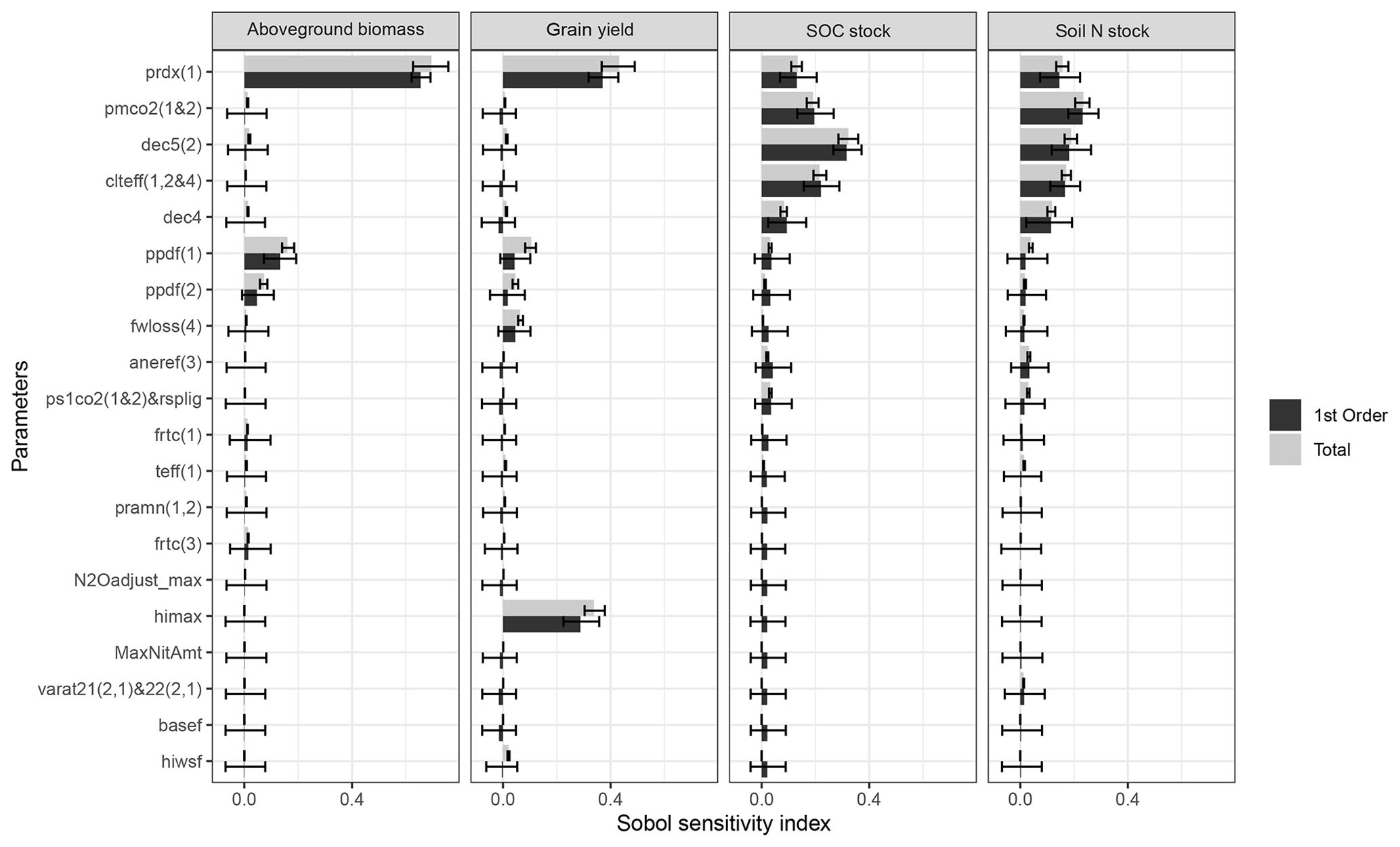
Figure 1 Results of the global sensitivity analysis of the most relevant DayCent model parameters. Parameter sensitivity was independently determined for the mean maize aboveground biomass, grain yield, and SOC and soil N stocks at the end of the simulation period. Only parameters with a Sobol sensitivity index >1 % are displayed.

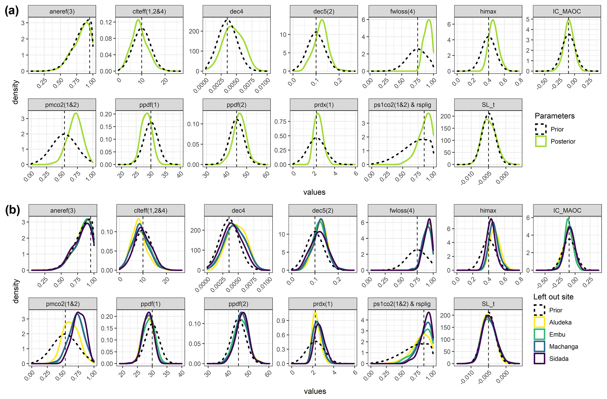
Figure 2 Prior compared to the posterior model parameter distribution resulting from the Bayesian model calibration of DayCent using (a) data from all sites combined (top) and (b) the leave-one-site-out cross-validation (bottom). The uncertainty ranges of the priors were based on the range of parameter values found in the literature and increased by a factor of 1.5 because DayCent was applied to the tropical site, while, historically, it was mostly calibrated based on temperate sites. Dashed vertical lines represent the values of the initially selected parameter set. The posterior distributions are based on all four study sites combined. For the description of the parameters, see Table 1.

3.2 Posterior parameter distributions from the Bayesian model calibration

Following the global sensitivity analysis, 13 selected model parameters were calibrated using Gaussian priors which were centered around the initial parameter value, with standard deviations according to the uncertainty ranges (Table 1). It should be noted that the presented calibrated parameter values in Table 1 correspond to the single best parameter set for all four sites combined (i.e., the parameter set that had the highest likelihood in the case of no cross-validation).

Compared to the range of the prior parameter sets, the ranges of the posterior parameter sets calibrated with data from all four sites changed significantly for the parameters fwloss(4) and pmco2(1&2); had a similar mean value but a more narrow distribution for the parameters IC_MAOC, prdx(1), and ps1co2(1&2)&rsplig; and changed slightly for the parameters dec4, dec5(2), ppdf(1), ppdf(2), and himax (Fig. 2). The posterior parameter sets of the leave-one-site-out cross-validations were largely in agreement with each other and with the posterior parameter sets calibrated with data from all four sites. The exception was the parameter pmco2(1&2), which was centered around 0.55 for the case that the Aludeka site was left out and around 0.70 for all other cases (Fig. 2).

The parameter that changed most strongly in the parameter sets calibrated with data from all four sites was the scaling factor for potential evapotranspiration (fwloss(4); from 0.75 to 0.94), thereby not including the initial value in the 95 % posterior credibility interval (0.81 to 0.99; Table 1). Also the CUE of metabolic litter was reduced (by an increase in pmco2(1&2) from 0.54 to 0.91 g g⁻¹), but the initial value was still within the 95 % posterior credibility interval (0.48 to 0.91 g g⁻¹). The turnover rates increased for both the slow SOM pool (dec5(2); from 0.10 to 0.13 g g⁻¹ yr⁻¹) and the passive SOM pool (dec4; from 0.0035 to 0.0060 g g⁻¹ yr⁻¹), which was however counterbalanced by a reduction in the effect of tillage on decomposition (clteff(1,2,&4); from 10 to 5), and all three of these parameters contained their initial values in the 95 % posterior credibility intervals. The maximum harvest index slightly increased (himax; from 0.40 to 0.43 g g⁻¹) and so did the potential production of maize per unit of light interception (prdx(1); from 2.25 to 2.62 g C m⁻² Ly⁻¹). Finally, the optimum temperature for maize growth decreased (ppdf(1); from 30 to 28.6 °C), while the maximum temperature for maize growth increased (ppdf(2); from 45 to 47.1 °C). Of the two parameters that translated measured MAOC into SOC in the passive SOM pool, only IC_MAOC was altered (from −0.1 to −0.02 g g⁻¹), but the initial value was still in the 95 % posterior credibility intervals (−0.25 to 0.06 g g⁻¹). Overall, the parameter correlations in the posterior parameter set across the four sites were low for soil-carbon-related parameters (around 0.4 at maximum), but stronger correlations existed between plant-productivity-related parameters (e.g., −0.7 between himax and prdx(1) and 0.58 between ppdf(1) and ppdf(2); Supplement Fig. S3).

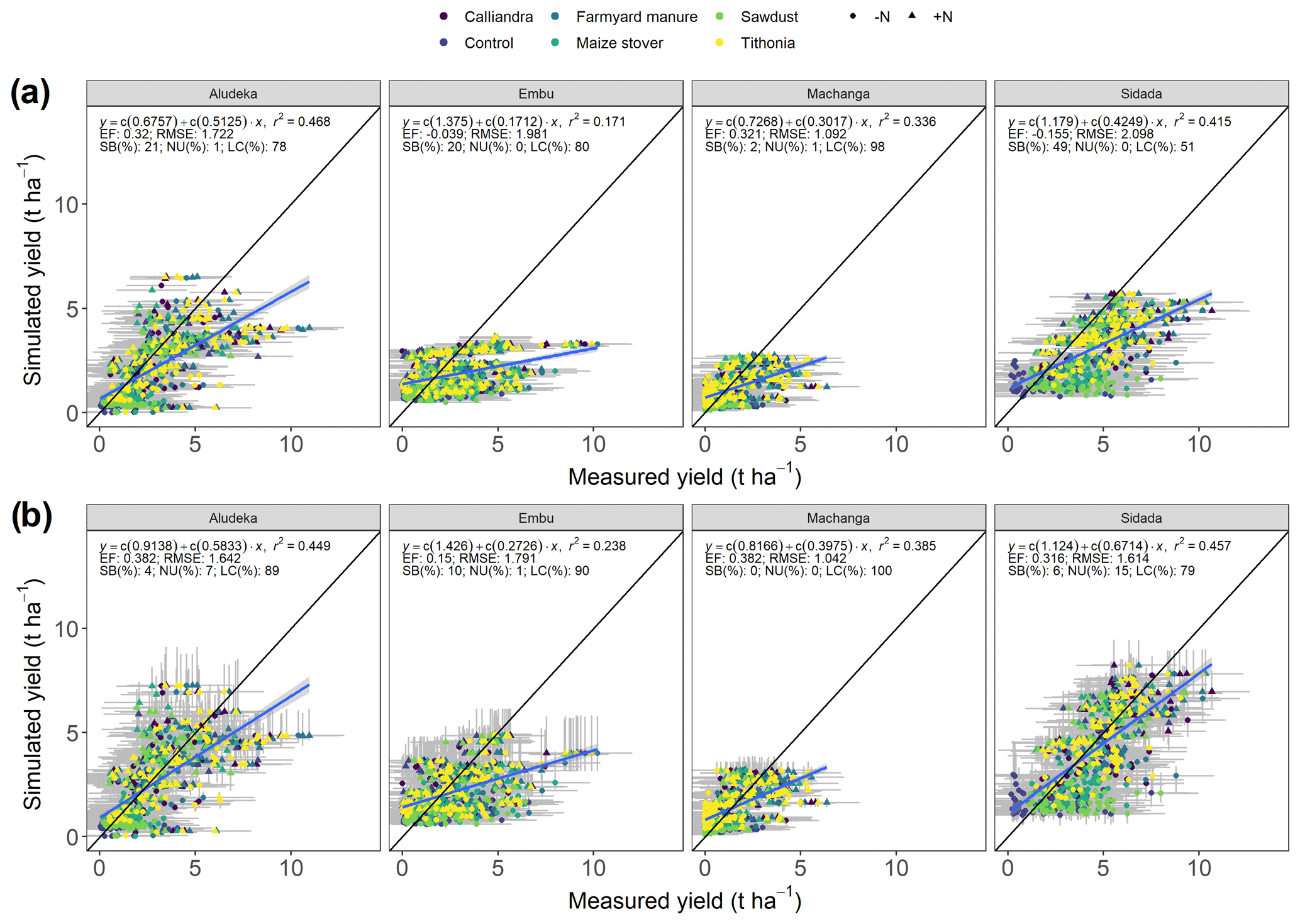
Figure 3 Simulated compared to measured maize grain yields at the four study sites for (a) the initial DayCent parameter set versus (b) the calibrated parameter set by leave-one-site-out cross-validation. The 2985 data points correspond to the observations from the experimental treatments over 32 to 38 seasons, depending on the site. Symbols represent the different organic-resource and chemical-nitrogen-fertilizer treatments. Grey bands show the 95 % confidence intervals of measured (horizontal) values and the 95 % credibility intervals of the posterior distribution (vertical). EF: Nash–Sutcliffe model efficiency, RMSE: root mean squared error, SB: squared bias, NU: non-unity slope, LC: lack of correlation. Model statistics across all sites are the following. Before calibration – EF: 0.358, RMSE: 1.757 t ha⁻¹, SB: 21 %, NU: 1 %, LC: 77 %. After calibration (with 27 % of measurements being in the 95 % credibility interval of the posterior) – EF: 0.503, RMSE: 1.545 t ha⁻¹, SB: 4 %, NU: 2 %, LC: 94 %.

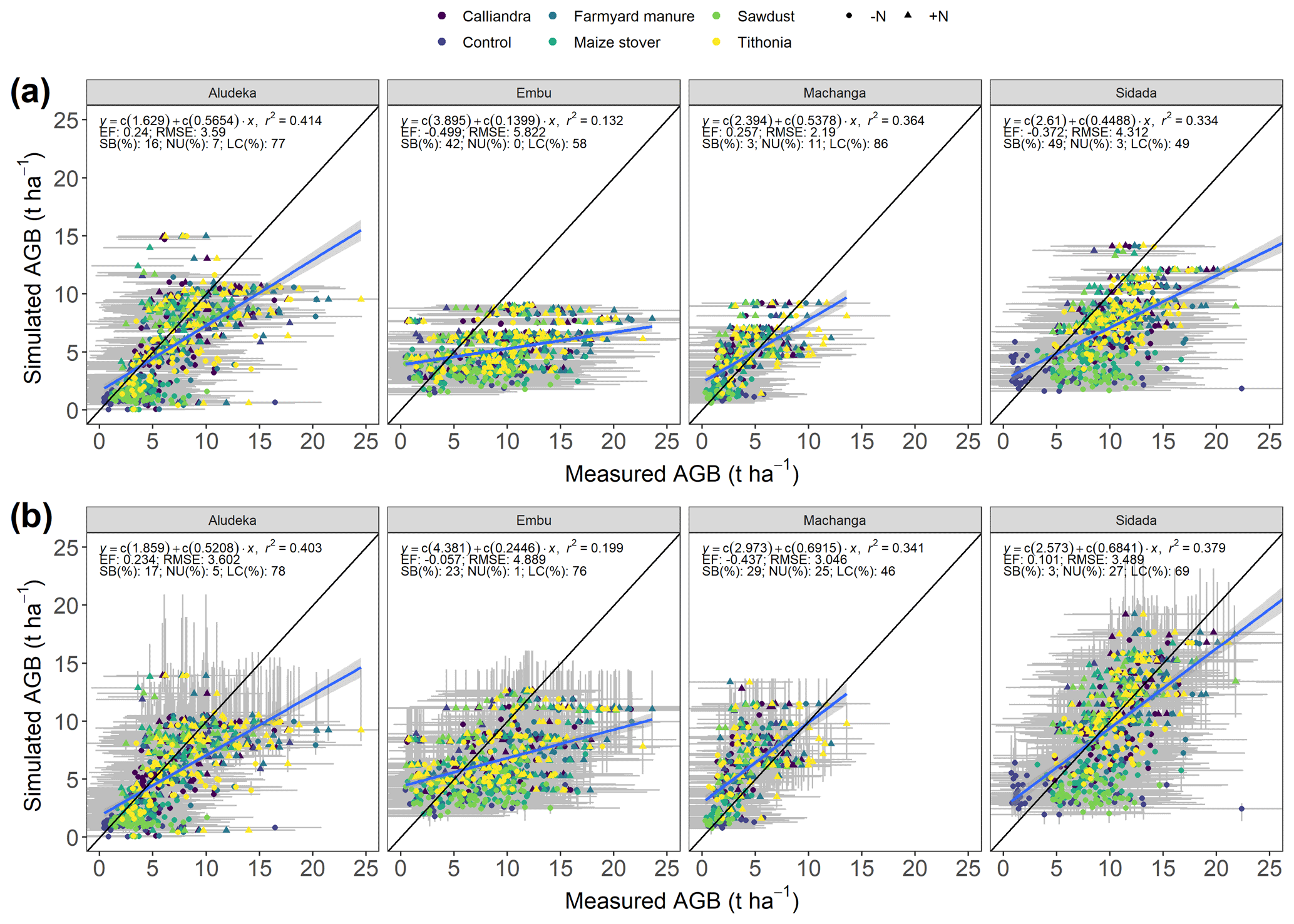
Figure 4 Simulated compared to measured maize aboveground biomass (AGB) at the four study sites for (a) the initial DayCent parameter set versus (b) the calibrated parameter set by leave-one-site-out cross-validation. The 2985 data points correspond to the observations from the experimental treatments over 32 to 38 seasons, depending on the site. Symbols represent the different organic-resource and chemical-nitrogen-fertilizer treatments. Grey bands show the 95 % confidence intervals of measured (horizontal) values and the 95 % credibility intervals of the posterior distribution (vertical). EF: Nash–Sutcliffe model efficiency, RMSE: root mean squared error, SB: squared bias, NU: non-unity slope, LC: lack of correlation. Model statistics across all sites are the following. Before calibration – EF: 0.033, RMSE: 4.392 t ha⁻¹, SB: 27 %, NU: 1 %, LC: 72 %. After calibration (with 36 % of measurements being in the 95 % credibility interval of the posterior) – EF: 0.231, RMSE: 3.915 t ha⁻¹, SB: 7 %, NU: 8 %, LC: 85 %.

3.3 Simulation of maize grain yields and aboveground biomass at harvest

While the overall variation in maize grain yields across sites and treatments could be captured to some extent with the initial model parameter set, a negative model efficiency was obtained for two sites (Fig. 3). With the leave-one-site-out cross-validation approach, the model efficiency for maize grain yields at the left-out site improved ubiquitously (i.e., from 0.32 to 0.38 at Aludeka, from −0.04 to 0.15 at Embu, from 0.32 to 0.38 at Machanga, from −0.16 to 0.31 at Sidada, and from 0.36 to 0.50 across all sites), and so did RMSE and bias. The same was true for the simulation of aboveground biomass (e.g., from 0.03 to 0.23 across sites; Fig. 4), with the exception of Machanga. Overall, biases in simulated grain yields were mostly eliminated through the model calibration, and biases in simulated aboveground biomass were eliminated at Sidada and reduced at Embu but increased at Machanga.

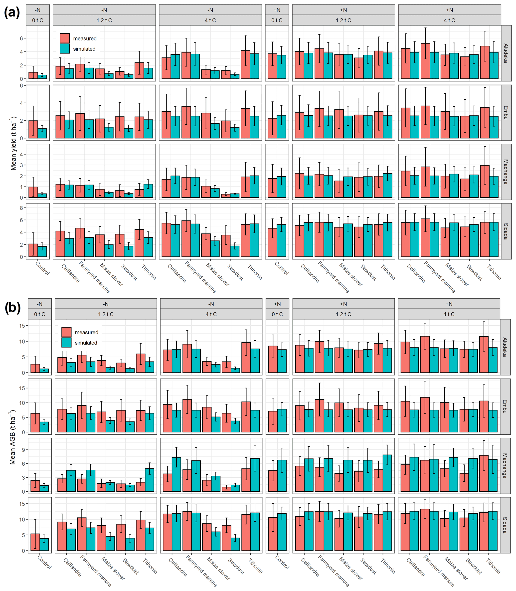
Figure 5 Bar plots of mean simulated and mean measured (a) maize grain yield and (b) aboveground biomass (AGB) from cross-validation. Error bars represent standard deviation.

While DayCent could not capture the full season-to-season variability in grain yields and aboveground biomass, the mean yields and aboveground biomass throughout the simulation period were simulated well for most treatments without the addition of mineral nitrogen (Supplement Fig. S4). The exception to this was the Embu site, where there was a systematic underestimation of yields in the +N treatments. Nonetheless, DayCent was able to acceptably simulate the variability in grain yields across sites by organic-resource and mineral-nitrogen-fertilizer treatment (model efficiencies between 0.30 and 0.54; with values for control −N (0.08) and sawdust −N (0.18) being the exception; Supplement Fig. S7). Interestingly, DayCent poorly distinguished the mean yields and aboveground biomass of treatments with high compared to very high rates of N inputs (i.e., the differences between the different organic resources and the control within the +N treatment). An additional test of the model sensitivity of mean yields to different levels of mineral nitrogen fertilizer in the control provided further insights into this (Supplement Fig. S5). In this test, the yields plateaued at rates of mineral nitrogen that were lower than the maximum N rates provided in the organic-resource and mineral-nitrogen-fertilizer treatments with mineral N and organic resources combined (up to >500 kg N yr⁻¹ or >250 kg N per growing season). At Machanga and Embu, simulated mean yields stopped increasing at around 100 kg N ha⁻¹ per growing season, which is less the 120 kg N ha⁻¹ per growing season in the control of +N. At Aludeka and Sidada, simulated mean yields stopped increasing at 200 to 250 kg N ha⁻¹ per growing season, but most of the response to N was below 120 kg N ha⁻¹ per growing season (Supplement Fig. S5). Although the mean yields in −N treatments with the high-quality inputs were well simulated, some of the low-quality input treatments at Aludeka and Sidada, namely maize stover and sawdust at 1.2 and 4 t C ha⁻¹ yr⁻¹, had lower simulated than observed mean yields in their −N treatments (Fig. 5). The same was true for the control −N at Aludeka, Embu, and Machanga.

3.4 Simulated SOC stocks in response to integrated soil fertility management

Similar to the simulation of maize grain yields, the simulations of changes in SOC stocks following the application of organic resources at different rates (1.2 and 4 t ha⁻¹ yr⁻¹) generally improved across sites by the leave-one-site-out cross-validation approach compared to using the initial model parameter set (Fig. 6). The improvement was even stronger when compared to DayCent simulations with the default CUE value for the structural pool (these had a negative model efficiency at all four sites; Supplement Fig. S6). While Aludeka experienced an improved but negative model efficiency for simulated changes in SOC stocks with the leave-one-site-out cross-validation (from −4.17 to −0.90), the model efficiencies at Embu and Sidada were positive in the initial parameter set and improved with calibration (from 0.53 to 0.54 at Embu and from 0.47 to 0.58 at Sidada). Also across sites, the model efficiency (computed without Machanga) improved considerably from 0.36 to 0.55 following calibration. As expected, Machanga, for which the SOC stock data had been removed from the calibration dataset due to soil erosion at this site, still exhibited a poor model efficiency after calibration (−1.9 compared to −4.8 before calibration). DayCent performed well in simulating the variability in the changes in SOC stocks across sites, evaluated by organic-resource and mineral-nitrogen-fertilizer treatment (also computed without Machanga). With the exception of the treatments farmyard manure ± N, maize stover ± N, and sawdust −N model efficiencies were between 0.51 and 0.79 (with RMSE between 3.2 and 4.3 t ha⁻¹; Supplement Fig. S8) with the highest performance for the control +N (0.79) and control −N (0.69) treatments. The other treatments still had positive model efficiencies (0.15 to 0.42), but the SOC losses of the farmyard manure treatments were overestimated (EF of 0.15 for −N, 0.29 for +N, RMSE of 5.1 and 5.3).

While SOC changes were well captured in the control treatments across all sites, it should be noted that the increases in SOC stocks in the treatment receiving 4 t C ha⁻¹ yr⁻¹ were overestimated at Aludeka (Supplement Fig. S9). As a result, the posterior credibility intervals of simulated SOC stocks matched well with measured SOC stocks of Embu and Sidada but not with those of Aludeka (Fig. 7). The difference between the 4 t C ha⁻¹ yr⁻¹ input and the control treatments were generally well simulated, but the fact that Machanga, the other sandy site, could not be used in the calibration due to erosion likely contributed to the poorer performance of the sandy site in Aludeka.

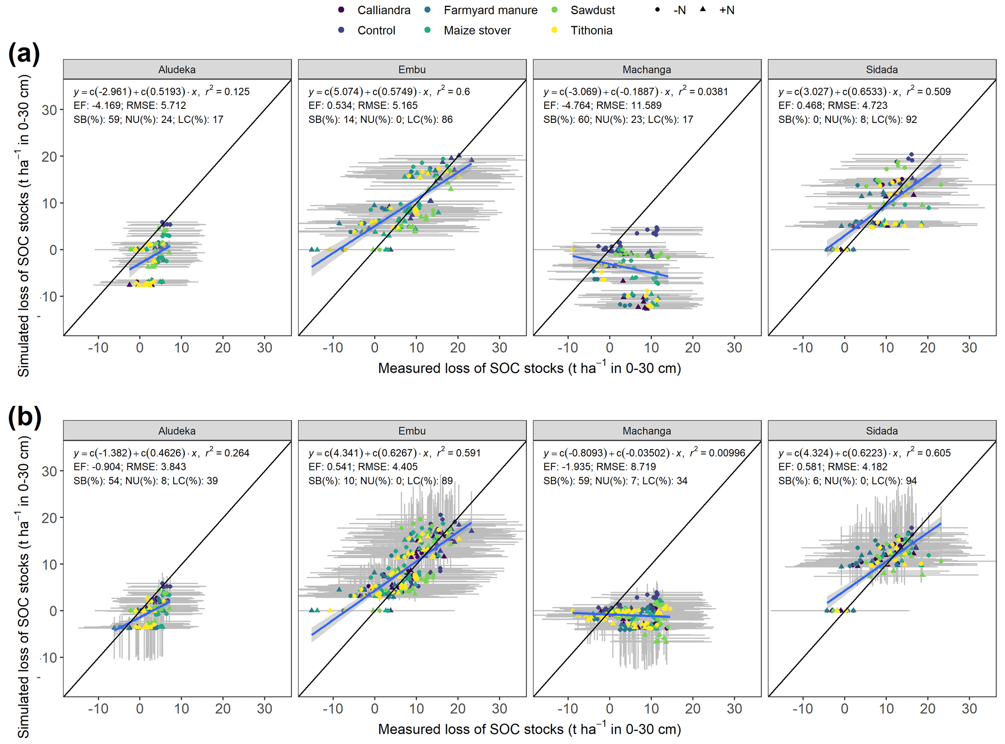
Figure 6 Simulated compared to measured changes in SOC stocks since the start of the experiment at the four study sites for (a) the initial DayCent parameter set versus (b) the calibrated parameter set by leave-one-site-out cross-validation. The 724 data points correspond to the observations from the experimental treatments over 32 to 38 seasons, depending on the site. Symbols represent the different organic-resource and chemical-nitrogen-fertilizer treatments. Grey bands show the 95 % confidence intervals of measured (horizontal) values and the 95 % credibility intervals of the posterior distribution (vertical). EF: Nash–Sutcliffe model efficiency, RMSE: root mean squared error, SB: squared bias, NU: non-unity slope, LC: lack of correlation. Model statistics across all sites except Machanga (from which SOC data was excluded in the calibration process due to strong erosion). Before calibration – EF: 0.364, RMSE: 5.199 t ha⁻¹, SB: 1 %, NU: 22 %, LC: 77 %. After calibration (with 45 % of measurements being in the 95 % credibility interval of the posterior) – EF: 0.548, RMSE: 4.22 t C ha⁻¹, SB: 1 %, NU: 11 %, LC: 89 %.

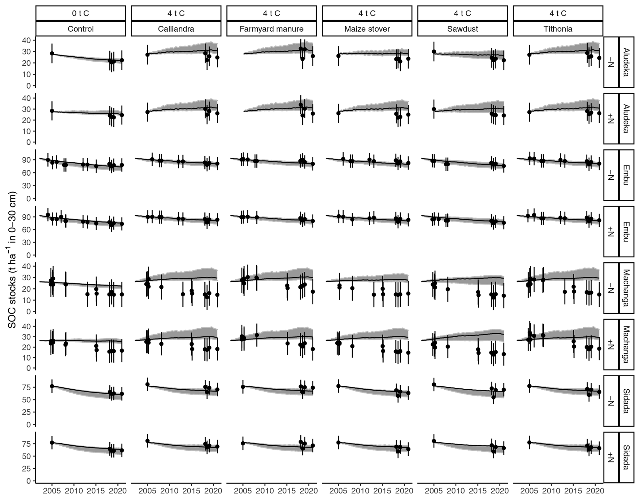
Figure 7 Measured (dots) versus simulated SOC stocks over time at the four study sites for the different organic-resource and chemical-nitrogen-fertilizer treatments. Error bars represent 95 % confidence intervals for measured data; the solid black line represents the simulation by the best parameter set. Grey bands represent the 95 % credibility intervals of the model posterior simulations, calibrated by leave-one-site-out cross-validation. Note that due to intense soil erosion, data from Machanga were not used in the calibration process.

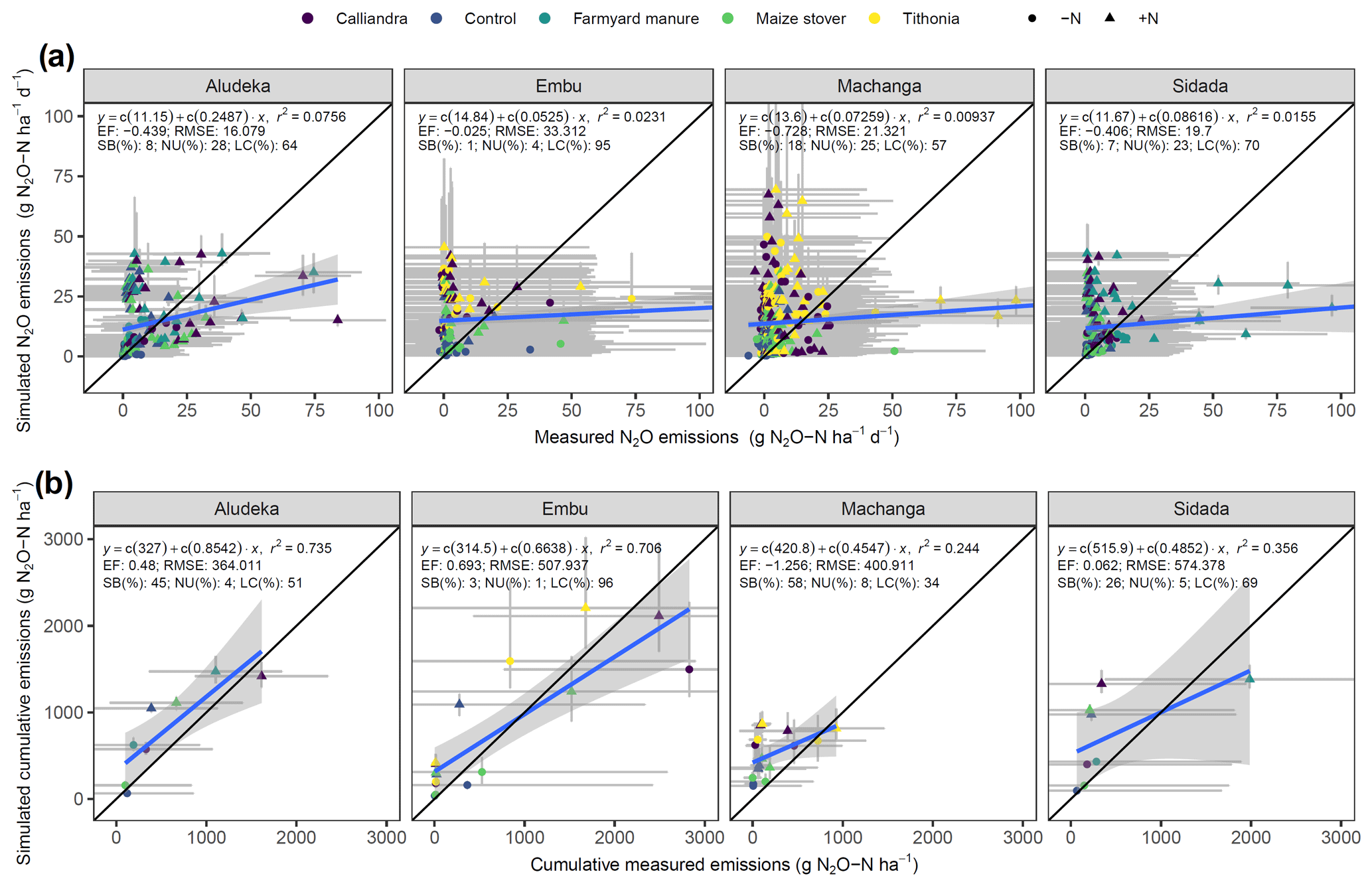
Figure 8 Simulated compared to measured N₂O emissions at the four study sites for the different organic-resource and chemical-nitrogen-fertilizer treatments, based on the calibrated parameter set using leave-one-site-out cross-validation. Displayed are the measured versus modeled values per treatment for (a) the days where measurements were conducted and (b) the mean of cumulative flux measurements per season using the trapezoid method. The 808 data points (a) correspond to the daily measurements from the experimental treatments over one to two seasons, depending on the site. Symbols represent the different organic-resource and chemical-nitrogen-fertilizer treatments. Error bars represent 95 % confidence intervals (measurements) and credibility intervals (simulations). Note that the credibility intervals are only informed by yield, SOC, and harvest index data and therefore do not represent the full uncertainty in N₂O emissions. EF: Nash–Sutcliffe model efficiency, RMSE: root mean squared error, SB: squared bias, NU: non-unity slope, LC: lack of correlation.

3.5 Simulated N₂O emissions and GHG balance

The negative model efficiencies and the absence of correlation between observed and simulated daily N₂O values indicated that model performance for daily N₂O emissions was poor (Fig. 8). While treatments with higher N loads had both higher simulated and measured N₂O fluxes compared to those with lower loads, the peaks of N₂O emissions were often simulated on different dates than the measurements. This was most noticeable in +N treatments (Supplement Fig. S10). Conversely, the simulated cumulative N₂O emissions per season were in a better agreement with the measured values. All sites, except Machanga, showed positive model efficiencies (highest at Embu, 0.69; lowest at Sidada, 0.06) but generally underestimated the uncertainty around cumulative N₂O emissions (Fig. 8). Additionally, the correlation between simulated and measured N₂O emissions was notably higher for the cumulative emission fluxes than for daily fluxes (R² of 0.74 for Aludeka, 0.7 for Embu, and 0.36 for Sidada, compared to an R² value of close to 0 for daily fluxes). Furthermore, despite some bias at Aludeka and Sidada, most of the error in seasonal N₂O emissions was not systematic (i.e., LC of 51 %–96 %).

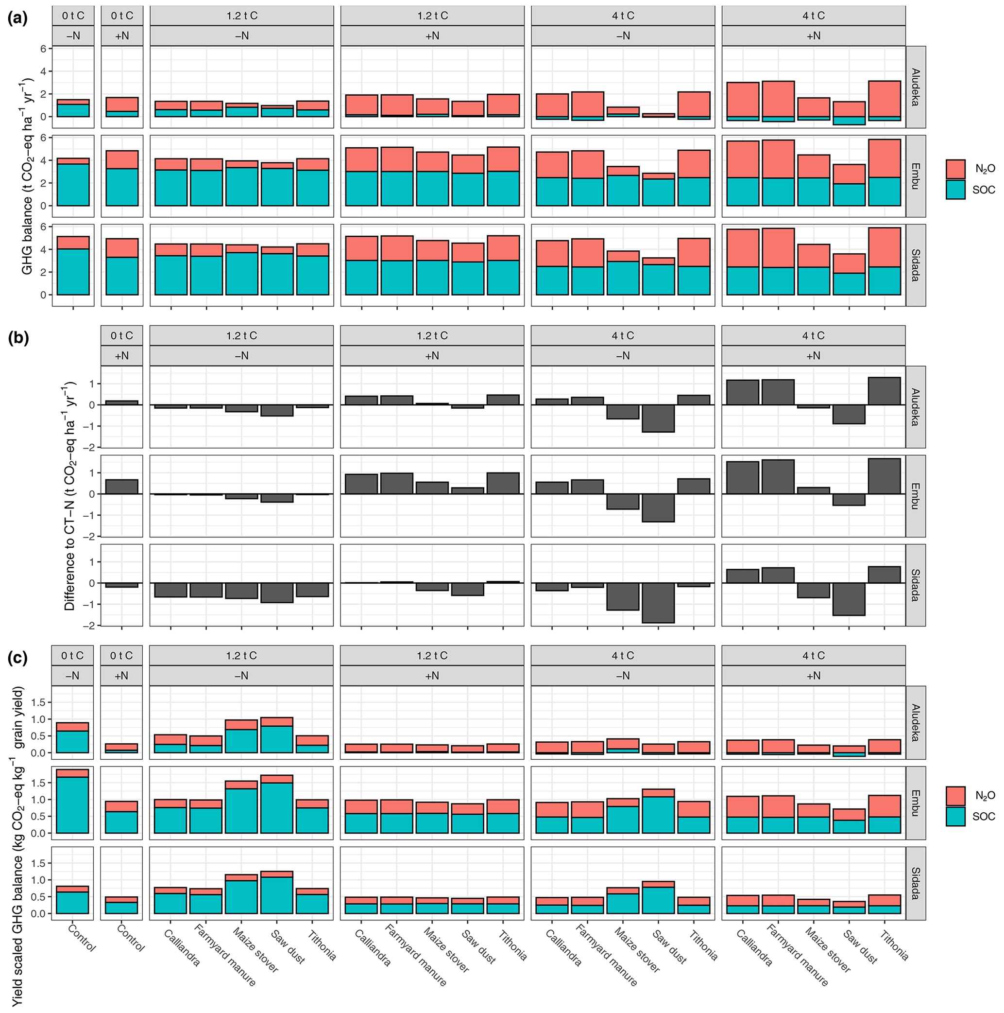
Figure 9 Cumulative simulated greenhouse gas (GHG) balance of N₂O emissions and CO₂ emissions due to the loss of SOC at the four study sites for different organic-resource and chemical-nitrogen-fertilizer treatments combined throughout the simulated period (16 years for Aludeka and Sidada, 19 years for Embu and Machanga). Displayed are the (a) GHG balance per area of land and year, (b) difference in GHG balance per area of land and year to a no-input treatment, and (c) yield-scaled GHG balance. The GHG balance is expressed in CO₂ equivalent over a 100-year horizon.

The simulated changes in SOC and seasonal N₂O emissions revealed a positive GHG balance for all treatments at all sites (Fig. 9a). Yet, the magnitude of emissions, as well as the relative contributions of N₂O and CO₂, differed strongly between sites and treatments. For instance, in the control −N treatment, emissions ranged from 1.5 t CO₂ eq. ha⁻¹ yr⁻¹ at Aludeka to 5 t CO₂ eq. ha⁻¹ yr⁻¹ at Sidada. The relative contribution of N₂O also differed strongly by site. At Aludeka, for example, all positive GHG balance values in the 4 t C ha⁻¹ yr⁻¹ treatments receiving farmyard manure, Tithonia, and Calliandra came from N₂O, while SOC acted as a sink of GHG. In contrast, at Sidada and Embu, most treatments had between a third and half of their GHG balance associated with N₂O emissions, with the remainder attributed to SOC losses. Compared to the control −N treatment, all organic-resource treatments in the −N treatments were simulated to have lower emissions at inputs of 1.2 t C ha⁻¹ yr⁻¹ (Fig. 9b). Yet, when including the 4 t C ha⁻¹ yr⁻¹ and the +N treatments, the changes ranged from an increase of around 1.5 t CO₂ eq. ha⁻¹ yr⁻¹ to a reduction of 2 t CO₂ eq. ha⁻¹ yr⁻¹. Embu was the site where the addition of mineral N (+N treatment) led to the strongest increase in simulated GHG balance compared to the control −N treatment.

Finally, there were site- and treatment-specific differences in the yield-scaled GHG balance. The treatment control of −N, maize stover −N, and sawdust −N had the highest simulated emissions per kilogram maize grain yield across sites (0.8 to 1.8 kg CO₂ equivalent per kg yield). In contrast, the farmyard manure, Calliandra, and Tithonia treatments at inputs of 1.2 t C ha⁻¹ yr⁻¹ in the +N treatment and at 4 t C ha⁻¹ yr⁻¹ in both −N and +N treatments tended to have the lowest simulated emissions at all sites (around 0.3, 1, and 0.6 kg CO₂ equivalent per kg yield at Aludeka, Embu, and Sidada, respectively).

4 Discussion

4.1 Robustness of the Bayesian calibration shown by cross-validation

As shown by the leave-one-site-out cross-validation (Figs. 3 and 4), the Bayesian calibration considerably improved the predictive capability of DayCent for maize grain yield, aboveground biomass, and changes in SOC stocks across sites. The model evaluation statistics from this calibration were comparable to those reported in recent publications that also combined the predictions of crop yield and SOC (Necpalova et al., 2018; Levavasseur et al., 2021; Nyawira et al., 2021). However, while these studies generally showed a better simulation of crop yield than SOC, our study diverged. We found that while better yield simulations compared to SOC simulations were evident at the Aludeka and Machanga sites with soils of low clay content, the results were different at the Embu and Sidada sites with clay-rich soils. Here, SOC stock changes were more accurately simulated than maize grain yield. This, together with the fact that the simulation of aboveground biomass worsened at two sites as a result of the calibration (Fig. 4), suggests that no single best parameter set exists for the current version of DayCent to accurately represent the conditions at all four sites. In that regard, the discrepancy between the sites with clay-rich and clay-poor soils could indicate that DayCent insufficiently includes soil textures effects on nutrient availability and SOC formation. Yet, drawing definitive conclusions from just four sites is probably not warranted. In the absence of data from more sites, it is preferable to apply the full range of possible parameter sets that are supported by the available data (Mathers et al., 2023) rather than using only the single best parameter set.

Because our calibration shows a good model fit with observed mean yields and changes in SOC stocks across sites, with no overall major bias (positive EF and errors mostly consisting of LC), the parameter set, especially the full posterior, appears suitable for upscaling of model simulations. Specifically, the yields of the ISFM treatments applying farmyard manure, Calliandra, and Tithonia were simulated well, both with and without the addition of mineral nitrogen fertilizer (Supplement Fig. S7). The changes in SOC stocks for the control, Calliandra, and Tithonia treatments were also simulated well across sites, while DayCent underestimates the SOC buildup from farmyard manure treatments (Supplement Fig. S8). However, one should keep in mind that the season-to-season yield variability is captured less accurately than the mean yields (lower RMSE) and that changes in SOC are better represented at sites with clay-rich soils than those with clay-poor soils. Because the model calibration and evaluation were performed at sites with diverse characteristics, it is reasonable to assume that DayCent, when applied to sites with similar climate and soil conditions, will provide satisfactory results with similar model uncertainties and errors. In that respect, while the leave-one-site-out cross-validation made efficient use of data for model evaluation, further model upscaling should apply the full posterior model parameter set including all sites (Fig. 2). In that case, a computationally inexpensive exercise would use only the single best parameter set (Table 1), while the full posterior parameter set should be used to get estimates of the posterior credibility intervals for changes in SOC stocks.

4.2 Bayesian calibration shows uncertainty in model parameters

To estimate the potential yield and long-term sustainability of cropping systems without major bias using biogeochemical models, region-specific model calibrations are needed (Rattalino Edreira et al., 2021; Yang et al., 2021). Therefore, while previous studies have simulated crop productivity under ISFM and similar practices with the default parameter values (e.g., Nezomba et al., 2018; Nyawira et al., 2021), the results of our study underscore the importance of a local calibration, especially when simulations are done with a single parameter set. On the one hand, the similar ranges of the prior and posterior model parameter sets for SOC-decomposition-related parameters (i.e., clteff(1,2&4), dec4, dec5(2)) indicate that the included prior knowledge about DayCent parameters from recent Bayesian calibration studies (Gurung et al., 2020; Yang et al., 2021; Mathers et al., 2023) represent good parameter estimates for a tropical setting. On the other hand, the CUE values of both metabolic litter (centered around 25 % with pmco2(1&2) around 0.75) and structural litter (centered around 10 % with ps1co2(1&2)&rsplig around 0.9) are low compared to the default values. This indicates the difficulty in stabilizing the organic-resource additions into SOM at the tropical soils of these four long-term experiments. Both parameters (pmco2(1&2) and ps1co2(1&2)&rsplig) are even higher than in a recent study by Mathers et al. (2023). However, because these values had reached their predefined upper boundary limit in the study by Mathers et al. (2023), our CUE values might even be representative of temperate and not just for the tropical conditions of Kenya. In general, including prior knowledge about model parameter values from similar studies substantially improves model performance compared to using default parameter values (e.g., see the poor model performance without including prior knowledge on ps1co(1&2)&rsplig; Supplement Fig. S6). In fact, the aligning turnover rates of the slow and passive SOM pools with those derived for temperate conditions (Gurung et al., 2020) indicate that the DayCent temperature function is well suited to handle the faster SOM turnover under tropical conditions.

It is important to note that our sites were under natural vegetation (i.e., forest) or fallow until relatively shortly before the establishment of the experiments (Laub et al., 2023a). Consequently, upon the start of cultivation, erosion and potentially accelerated decomposition (due to soil disturbance) occurred, and SOC had likely not yet reached a new equilibrium with C inputs from maize cultivation. Therefore, C loss is the dominant process occurring at the sites. The good simulations of the strong SOC changes in the control treatments when using MAOC initialized SOM pools, a method not commonly used with DayCent, further supporting suggestions to move away from purely conceptual SOM pools (Abramoff et al., 2018; Laub et al., 2024). Such conceptual pools require many assumptions about the initial vegetation and soil conditions (e.g., in the spin-up modeling or estimation of SOM pool distribution). In fact, the high uncertainty about initial vegetation, as well as time and management since site conversion, was a major reason to move away from the model spin-up and site history run usually typically done with DayCent. Thus, our study provides additional support to modify DayCent, incorporating measurable SOM pools (e.g., Dangal et al., 2022).

Nevertheless, soil property maps, which would be needed to initialize measurable SOM pools at scale, are also subject to uncertainty. For example, differences between different SOC maps used in model initialization propagate into differences in the changes in SOC stocks (Zhou et al., 2023). It was shown that uncertainty in the simulated effect of a soil management practice on the difference in SOC stocks compared to a counterfactual is lower than the uncertainty in the simulated temporal development of SOC stocks (Zhou et al., 2023). Therefore, it may be best practice to work with a baseline and an improved scenario. Both spin-up and SOC map initialization have their shortcomings, and in the end the model user must make an informed decision on which initialization method they consider subject to less uncertainty, based on which data are locally available.

The similarity of our DayCent model calibration with that of Gurung et al. (2020) and earlier studies, despite using different model initialization approaches, indicates the broad applicability of DayCent. It suggests that the SOM turnover and maize traits in DayCent are representative of temperate to tropical conditions. The adjustments made to the values of optimal and maximum temperature for maize growth (ppdf(1) and ppdf(2)) could be attributed to the local maize varieties that are adapted to the higher temperatures in Kenya. For example, Yang et al. (2021) conducted a region-specific Bayesian model calibration of the DayCent maize growing parameters and found ppdf(1) to vary between 26 and 32 °C, a range similar to our posterior. However, the differences in model performance by site shows that the broad representativeness of DayCent comes at the cost of model simplification and site-specific model performance. A main reason for this may be that DayCent model formalisms do not include the latest mechanistic understandings of the role of microbes in SOM decomposition (Laub et al., 2024) and the sorption kinetics of carbon to minerals for SOM protection (Abramoff et al., 2018; Ahrens et al., 2020). Additionally, DayCent does not fully consider that a lot of stabilized SOC is formed by microbes from metabolic and not structural litter (Cotrufo et al., 2013; Kallenbach et al., 2016). For example, it was recently demonstrated that the Millennial model, which includes measurable SOM pools and improved kinetics of carbon sorption, better predicts SOC stocks at the global scale than the CENTURY model, which has conceptual SOM pools (Abramoff et al., 2022). While model calibration can compensate for deficiencies in mechanistic accuracy at a single site (Laub et al., 2024), this is likely not possible across sites with different conditions.

An interesting observation is that while the model bias for the mean maize yield was treatment specific (i.e., the mean yields of +N treatments of farmyard manure at 4 t C ha⁻¹ yr⁻¹ at all sites and of Tithonia at the same rate at all sites but Sidada were underpredicted by DayCent), the bias for SOC stocks was mostly site specific (i.e., SOC formation at Aludeka of 4 t C ha⁻¹ yr⁻¹ was overpredicted). A potential explanation for this site-specific bias for SOC is the fact that DayCent was developed under the paradigm of SOM formation occurring mainly from recalcitrant humic compounds in the soil. Alternatively, it might indicate that soil texture alone is insufficient to explain the mineralogy-driven storage potential of SOC (e.g., Reichenbach et al., 2021; Mainka et al., 2022) or that, because Machanga SOC stocks were not used in the calibration due to erosion, SOC changes at clay-rich sites cannot inform SOC changes at sandy sites like Aludeka. Finally, our model sensitivity test of inputs of mineral nitrogen suggests that the maize yield bias at high N is due to DayCent's inability to capture yield increases above 100–150 kg N ha⁻¹ per season at the four sites (Supplement Fig. S5); the +N treatments of Tithonia, Calliandra, and farmyard manure at 4 t C ha⁻¹ yr⁻¹ supplied on average >250 kg N ha⁻¹ per season. Here, it should be noted that DayCent does not include other potential beneficial effects of organic-resource treatments, such as increased pH from farmyard manure application (Xiao et al., 2021; Mtangadura et al., 2017) or improved water infiltration of treatments that maintain SOC stocks compared to those that reduce them.

4.3 N₂O emissions and GHG balance

In general, the poor match between observed and measured daily N₂O emissions (Supplement Fig. S10) illustrates the difficulty of simulating the timing of microbial processes, through which nitrate (NO₃⁻) is converted to N₂ and N₂O gases, with models of intermediate complexity such as DayCent. One reason is the poor representation of soil moisture dynamics by the “tipping-bucket” soil water balance approach and that soil gas diffusivity is not explicitly simulated (Zhang and Yu, 2021; Wang et al., 2020). However, the fact that cumulative N₂O emissions were better simulated than daily emissions, that there was no systematic under- or overprediction of cumulative N₂O emissions, and that simulated N₂O emissions were within the uncertainty range of measured N₂O emissions demonstrates the suitability of DayCent to represent average N₂O emissions with the current calibration. Nonetheless, the fact that the uncertainty around predicted cumulative N₂O emissions was lower than the uncertainties in the measurements indicates that the posterior, which was only calibrated with yield, SOC, and harvest index data, underestimates the uncertainty around N₂O emission predictions. Thus, although DayCent's simulations of N₂O emissions are superior to using emission factor approaches (dos Reis Martins et al., 2022), simulating N₂O emissions remains challenging and highly uncertain due to the complexity of the processes involved and their high temporal and spatial variability. Given the limited bias in simulating SOC changes and cumulative N₂O emissions shown, the DayCent simulations provide a reasonable first estimate of the GHG balance. Nevertheless, the contributions of N₂O emissions to the GHG balance of up to 100 % (at Aludeka) and between 10 % to 60 % (at the other sites; Fig. 9) are subject to high uncertainty, as evident from the measurements.

Despite this unresolved uncertainty, our modeling results show that all ISFM options in a maize monocropping system have a net positive GHG balance, aligning with the prevalent trend of SOC losses in recently established (<50 years) maize systems in SSA (Sommer et al., 2018; Laub et al., 2023a). The findings also support the postulate that closing yield gaps in SSA will increase N₂O emissions per area of land (Leitner et al., 2020). However, the large differences in the yield-scaled GHG balance between treatments, such as the 30 % to 60 % lower yield-scaled GHG balance in the FYM 1.2 +N treatment compared to the control −N treatment across the sites, indicate that ISFM has the potential to produce crops with relatively lower GHG emissions than no- or low-input systems and that the calculation of emissions per unit of food is preferable to the calculation per land area (Clark and Tilman, 2017). Specifically, the ISFM treatments with low-emissions and high yields, such as FYM 1.2 +N, which produces between 2 and 4 t of yield per season at emissions of between 0.3 and 1 kg CO₂ equivalent per kg yield, are a suitable mitigation practice compared to the control treatment with few or no inputs of organic and/or chemical fertilizer. Consequently, sustainable intensification and mitigation of greenhouse gases can go hand in hand.

4.4 DayCent is suitable to upscale simulations of “real” ISFM but has a limited sensitivity to high nitrogen inputs

Because mean maize yields across sites were reasonably well represented by the calibrated version of DayCent, it can be used for upscaling to predict the potential impact of ISFM in lowering yield gaps at national levels. However, the plateauing of mean yields at high nitrogen loads (Supplement Fig. S5) indicates that DayCent may not be suitable for estimating maximum achievable yields (e.g., Ittersum et al., 2016) and should thus be restricted to yield predictions for medium nitrogen input levels. Given that the historical rates of nitrogen fertilizer application in Kenya are less than 50 kg N ha⁻¹ (World-Bank, 2021a), the model seems suitable to simulate the effect of implementing “realistic” ISFM practices, which target maximum nitrogen use efficiency (Vanlauwe et al., 2010), with N input rates considerably below the maximum N rates used in the field experiments of this study (e.g., 80 kg N per season; Mutuku et al., 2020). At all sites, the prediction of mean maize yields was reasonably well for Calliandra, Tithonia, and farmyard manure treatments at 1.2 and 4 t C ha⁻¹ in the −N treatment, as well as for CT +N, i.e., all treatments that supply nitrogen at the desired rate for ISFM. Also, the variability in yields and SOC stock changes per treatment across sites was simulated well for Calliandra, Tithonia, and farmyard manure in both +N and −N treatments (with changes in SOC being simulated a bit worse in farmyard manure treatments; Supplement Figs. S7 and S8). While this shows the general capability of DayCent to simulate differences in yields and SOC changes between sites as a function of organic-resource composition, it also shows that DayCent cannot capture the better performance of farmyard manure compared to Calliandra and Tithonia treatments when only considering C, N, and lignin contents. Overall, simulated mean maize yields at medium nitrogen levels are likely representative of the achievable yield through ISFM. In summary, the model calibration seems suitable for assessing the long-term effects of relevant ISFM practices on soil fertility, maize yield, and GHG emissions as well as their trade-offs, given the good representation of mean yield potential and SOC changes by the model. Nevertheless, since year-to-year yield variations were not captured well by DayCent, it remains uncertain how effectively the current model calibration can simulate scenarios of climate change, where temperature and precipitation patterns will become more erratic. In the absence of major pests (which in the experiments were controlled), the variations in seasonal precipitation and temperature are responsible for these differences, and if these are not well represented, the applicability of DayCent beyond the climatic range that it was calibrated for is questionable.

5 Conclusions

In this study, we demonstrated the effectiveness of simultaneously calibrating the SOM and plant modules of DayCent to simulate maize productivity and changes in SOC stocks under integrated soil fertility management (ISFM) in Kenya. Using a Bayesian calibration approach, our study shows the importance of using a local calibration and of choosing correct prior values for model parameters. Although the initial DayCent parameterization represented the tropical conditions in Kenya acceptably, the overall model performance for maize grain yield, aboveground biomass, and SOC stock changes was improved after calibration using local data. Furthermore, while parameters related to SOM turnover were comparable to previous studies, a lower carbon use efficiency of applied organic resources (higher values of CO₂-loss-related parameters) compared to previous studies highlighted the difficulty in building new SOC stocks in the studied tropical soils. Our leave-one-site-out cross-validation showed that the calibration-derived parameter set is robust for upscaling the model simulations to larger areas in Kenya, particularly when applying the full posterior parameter set. At the same time, while mean maize grain yields were well simulated, the year-to-year yield variability raised concerns about the model's ability to capture the short-term effects of climate change adequately. Finally, while no ISFM treatment was predicted to act as a net sink of greenhouse gases, treatments with high and intermediate yields exhibited the lowest yield-scaled emissions.