Position-specific kinetic isotope effects for nitrous oxide: a new expansion of the Rayleigh model

Nitrous oxide (N₂O) is a potent greenhouse gas and the most significant anthropogenic ozone-depleting substance currently being emitted. A major source of anthropogenic N₂O emissions is the microbial conversion of fixed nitrogen species from fertilizers in agricultural soils. Thus, understanding the enzymatic mechanisms by which microbes produce N₂O has environmental significance. Measurement of the ¹⁵N $/$ ¹⁴N isotope ratios of N₂O produced by purified enzymes or axenic microbial cultures is a promising technique for studying N₂O biosynthesis. Typically, N₂O-producing enzymes combine nitrogen atoms from two identical substrate molecules (NO or NH₂OH). Position-specific isotope analysis of the central (N^α) and outer (N^β) nitrogen atoms in N₂O enables the determination of the individual kinetic isotope effects (KIEs) for N^α and N^β, providing mechanistic insight into the incorporation of each nitrogen atom. Previously, position-specific KIEs (and fractionation factors) were quantified using the Rayleigh distillation equation, i.e., via linear regression of δ¹⁵N^α or δ¹⁵N^β against [$-f\ln f/(\mathrm{1}-f)$], where f is the fraction of substrate remaining in a closed system. This approach, however, is inaccurate for N^α and N^β because it does not account for fractionation at N^α affecting the isotopic composition of substrate available for incorporation into the β position (and vice versa). Therefore, we developed a new expansion of the Rayleigh model that includes specific terms for fractionation at the individual N₂O nitrogen atoms. By applying this Expanded Rayleigh model to a variety of simulated N₂O synthesis reactions with different combinations of normal, inverse, and/or no KIEs at N^α and N^β, we demonstrate that our new model is both accurate and robust. We also applied this new model to two previously published datasets describing N₂O production from NH₂OH oxidation in a methanotroph culture (Methylosinus trichosporium) and N₂O production from NO by a purified Histoplasma capsulatum (fungal) P450 NOR, demonstrating that the Expanded Rayleigh model is a useful tool in calculating position-specific fractionation for N₂O synthesis.

1 Introduction

Nitrous oxide (N₂O) is a greenhouse gas with a global warming potential approximately 300 times greater than that of CO₂ (100-year time horizon) (Stocker et al., 2013). In addition, N₂O is the primary source of stratospheric NO_x and is therefore a significant ozone-depleting substance (Ravishankara et al., 2009). Levels of atmospheric N₂O are increasing by an average of ∼ 0.29 % annually (Lan et al., 2022), primarily due to rising anthropogenic N₂O emissions, which comprise approximately 40 % of annual global N₂O emissions (Tian et al., 2020). In the US, at least 70 % of annual anthropogenic N₂O emissions result from agricultural practices, such as the application of nitrogen-containing fertilizer (e.g., ammonium and nitrate) to the field. Soil microbes can metabolize these nitrogen-containing compounds through processes such as nitrification and denitrification, producing N₂O either as a side product (nitrification), intermediate (complete denitrification), or end product (incomplete denitrification) (Kuypers et al., 2018). Understanding the underlying mechanisms of N₂O production for each metabolic pathway is critical for tracing and ultimately mitigating environmental N₂O emissions.

Many different types of enzymes catalyze N₂O formation in microbes. Examples of N₂O-producing enzyme families include cytochrome P460 (Caranto et al., 2016) and hydroxylamine oxidoreductase (Yamazaki et al., 2014) in nitrifiers, “bacterial” nitric oxide reductases (cNOR, qNOR, etc.) found in bacterial and archaeal denitrifiers, and fungal nitric oxide reductase (P450 NOR) from fungal denitrifiers (Yamazaki et al., 2014; Yang et al., 2014; Lehnert et al., 2018) as well as detoxifying enzymes such as flavodiiron nitric oxide reductases (Romão et al., 2016). Distinguishing among different sources of N₂O in the environment and identifying the relative contribution of each source are challenging and require a combination of analytical methods. One useful technique for N₂O source apportionment is stable isotope analysis. This method takes advantage of the fact that many physical and chemical processes, such as enzyme-catalyzed reactions, generally have slightly different rate constants for different isotopes of the same element (e.g., ¹⁴N and ¹⁵N). In an isotopically sensitive process, the isotope that reacts faster will be more prevalent (enriched) in the product relative to the substrate. Different processes generally have distinct patterns of isotopic enrichment and thus have unique isotopic signatures.

Stable isotope analysis is particularly useful for studying N₂O synthesis because the central (N^α) and outer (N^β) nitrogen atoms in N₂O are non-equivalent and non-exchangeable, and the isotope ratios of these two nitrogen atoms can be determined individually (Toyoda and Yoshida, 1999). These position-specific isotope ratios can aid in identifying which enzyme produces or which enzymes produce N₂O in microbial cultures under varying growth conditions (Sutka et al., 2003, 2004, 2006, 2008; Toyoda et al., 2005; Frame and Casciotti, 2010; Yamazaki et al., 2014; Haslun et al., 2018). Additionally, because isotopic enrichment is typically dependent on the rate-limiting step(s) of the enzyme-catalyzed reaction, analyzing the isotopic signatures of individual enzymes can provide valuable insights into each enzyme's catalytic mechanism.

Isotopic enrichment for a specific process can be quantified by determining a parameter known as the fractionation factor (${\mathit{\alpha }}_{\mathrm{p}/\mathrm{s}}$). For reactions with first-order kinetics, ${\mathit{\alpha }}_{\mathrm{p}/\mathrm{s}}$ is equal to the rate constant of the heavy isotope (k_H) divided by the rate constant for the light isotope (k_L). Because ${\mathit{\alpha }}_{\mathrm{p}/\mathrm{s}}$ values are typically close to 1, ${\mathit{\alpha }}_{\mathrm{p}/\mathrm{s}}$ is often converted to its per mil equivalent, the enrichment factor (${\mathit{\epsilon }}_{\mathrm{p}/\mathrm{s}}$) (Mariotti et al., 1981).

$$\begin{array}{}\text{(1)}& {\mathit{\epsilon }}_{\mathrm{p}/\mathrm{s}}=\left({\mathit{\alpha }}_{\mathrm{p}/\mathrm{s}}-\mathrm{1}\right)\cdot \mathrm{1000}\end{array}$$

Notably, ${\mathit{\alpha }}_{\mathrm{p}/\mathrm{s}}$ is also equal to the inverse of the kinetic isotope effect (KIE =k_L/k_H). The KIE and fractionation factor values for a specific reaction describe the isotopic preference of that reaction. Most commonly, the light isotope reacts faster than the heavy isotope (i.e., KIE >1), which is designated as a normal KIE. Conversely, when the heavy isotope reacts faster (KIE <1), the reaction is said to have an inverse KIE. If the heavy and light isotopes react at the same rate (KIE = 1), the reaction has no kinetic isotope effect.

Mariotti et al. (1981) derived an approximation of the Rayleigh distillation equation (hereafter referred to as the (standard) Rayleigh equation) that is frequently used to determine enrichment factors in closed systems (Eq. 2) (Mariotti et al., 1981).

$$\begin{array}{}\text{(2)}& {\mathit{\delta }}^{\mathrm{15}}{\mathrm{N}}^{\mathrm{p}}={\mathit{\delta }}^{\mathrm{15}}{\mathrm{N}}^{\mathrm{s}\mathrm{0}}-{\mathit{\epsilon }}_{\mathrm{p}/\mathrm{s}}\cdot {\displaystyle \frac{f\ln \left(f\right)}{\mathrm{1}-f}}\end{array}$$

Here, δ¹⁵N^p is the δ value of accumulated product (p) at time t, δ¹⁵N^s0 is the δ value of the substrate at t= 0, and f is the fraction of substrate remaining at time t (f = N^s $/$ N^s0). (The δ values are directly related to isotope ratios; see the “Isotope nomenclature” section below.) Notably, the Rayleigh equation is based on the assumption that the element of interest is transferred from the substrate to a single position (or equivalent positions) in the product.

The Rayleigh equation (Eq. 2) holds true for δ¹⁵N^bulk (the average of δ¹⁵N^α and δ¹⁵N^β) because the overall reaction can be thought of as the unidirectional conversion of two identical substrate molecules (e.g., two NO or two NH₂OH molecules) to one product molecule with two nitrogen atoms (2S→P₂). In the absence of side reactions, this means that δ¹⁵N^bulk can be calculated at any point during the reaction (i.e., for any value of f) as long as the δ value of the initial substrate (δ¹⁵N^s0) and the enrichment factor (ε_N-bulk) are known. In practice, the ε_N-bulk value for a specific enzymatic reaction is found by plotting δ¹⁵N^bulk versus [$-f\ln f/(\mathrm{1}-f)$]. Because it is assumed that changes in δ¹⁵N^bulk are due solely to the bulk kinetic isotope effect of the reaction in question, the slope of this plot (determined by linear regression) is the bulk enrichment factor (ε_N-bulk), and the y intercept corresponds to δ¹⁵N^s0.

Unfortunately, the relationship between δ¹⁵N^α, δ¹⁵N^β, and their corresponding enrichment factors is more complex because the two N atoms are non-exchangeable and both steps that incorporate NO (or NH₂OH) are potentially isotopically sensitive. In other words, fractionation at the α position alters the isotopic ratio of the remaining substrate (δ¹⁵N^s) that is available for incorporation into the β position, and vice versa. Thus, simply determining the change in δ¹⁵N^α (or δ¹⁵N^β) as a function of [$-f\ln f/(\mathrm{1}-f)$] over the course of the reaction (i.e., finding the slope of a Rayleigh plot via linear regression of δ¹⁵N^α or δ¹⁵N^β against [$-f\ln f/(\mathrm{1}-f)]$) is not an accurate method for calculating the enrichment factor for N^α (or N^β).

The complexity of calculating enrichment factors for a branched N₂O biosynthesis reaction can be demonstrated mathematically by substituting $\mathrm{1}/\mathrm{2}$ (δ¹⁵N^α+δ¹⁵N^β) for δ¹⁵N^p and $\mathrm{1}/\mathrm{2}$ (${\mathit{\epsilon }}_{\mathrm{N}-\mathit{\alpha }}+{\mathit{\epsilon }}_{\mathrm{N}-\mathit{\beta }}$) for ${\mathit{\epsilon }}_{\mathrm{p}/\mathrm{s}}$ in the Rayleigh equation (Eq. 2), yielding Eq. (3).

$$\begin{array}{}\text{(3)}& {\displaystyle \frac{\mathrm{1}}{\mathrm{2}}}\left({\mathit{\delta }}^{\mathrm{15}}{\mathrm{N}}^{\mathit{\alpha }}+{\mathit{\delta }}^{\mathrm{15}}{\mathrm{N}}^{\mathit{\beta }}\right)={\mathit{\delta }}^{\mathrm{15}}{\mathrm{N}}^{\mathrm{s}\mathrm{0}}-{\displaystyle \frac{\mathrm{1}}{\mathrm{2}}}\left({\mathit{\epsilon }}_{\mathrm{N}-\mathit{\alpha }}+{\mathit{\epsilon }}_{\mathrm{N}-\mathit{\beta }}\right){\displaystyle \frac{f\ln \left(f\right)}{\mathrm{1}-f}}\end{array}$$

Here, ε_N−α and ε_N−β stand for the isotopic enrichment factors for the α and β nitrogen atoms, respectively. Equation (3) can then be rearranged to solve for δ¹⁵N^α (Eq. 4).

$$\begin{array}{}\text{(4)}& \begin{array}{rl}{\mathit{\delta }}^{\mathrm{15}}{\mathrm{N}}^{\mathit{\alpha }}& =\mathrm{2}{\mathit{\delta }}^{\mathrm{15}}{\mathrm{N}}^{\mathrm{s}\mathrm{0}}+{\mathit{\epsilon }}_{\mathrm{N}-\mathit{\alpha }}\left(-{\displaystyle \frac{f\ln \left(f\right)}{\mathrm{1}-f}}\right)\\ & +{\mathit{\epsilon }}_{\mathrm{N}-\mathit{\beta }}\left(-{\displaystyle \frac{f\ln \left(f\right)}{\mathrm{1}-f}}\right)-{\mathit{\delta }}^{\mathrm{15}}{\mathrm{N}}^{\mathit{\beta }}\end{array}\end{array}$$

The underlying difficulty in using Eq. (4) is that for a given value of f, δ¹⁵N^α depends not only on δ¹⁵N^s0 and ε_N−α, but also on ε_N−β and the current δ¹⁵N^β value. Put another way, we have one equation and two unknowns (ε_N−α and ε_N−β).

To address this issue, we developed an expanded version of the Rayleigh model that includes specific terms for the individual nitrogen atoms in N₂O. To test the robustness of this new Expanded Rayleigh model, we generated simulated isotopic data for each of five different potential catalytic mechanisms for N₂O formation. For each N₂O synthesis scenario, the size and skewness of the simulated measurement error were varied, and 1000 simulated datasets were generated for each combination of error level and skewness type. We then applied the standard Rayleigh model and Expanded Rayleigh model to each dataset to determine ε_N-bulk, ε_N−α, and ε_N−β and compared the precision and accuracy of the two models. Finally, we compared the results of applying the standard Rayleigh model and Expanded Rayleigh model to previously published isotopic data.

2 Methods

2.1 Isotope nomenclature

The isotopic ratio, R, is defined as the abundance of the heavy isotope (¹⁵N) divided by the abundance of the light isotope (¹⁴N).

$$\begin{array}{}\text{(5)}& R={\displaystyle \frac{\mathrm{Heavy}\mathrm{isotope}}{\mathrm{Light}\mathrm{isotope}}}=\left(\mathrm{e}.\mathrm{g}.,{\displaystyle \frac{{}^{\mathrm{15}}\mathrm{N}}{{}^{\mathrm{14}}\mathrm{N}}}\right)\end{array}$$

In the case of nitrogen, ¹⁴N is naturally much more abundant than ¹⁵N (the atom percent of ¹⁵N in atmospheric N₂ (air) is 0.3663 ± 0.0004 %, so R = 0.0036765) (Junk and Svec, 1958; Mariotti et al., 1981; Skrzypek and Dunn, 2020). The R value of a sample is usually measured relative to that of a standard ($R_{\mathrm{sample}}/R_{\mathrm{standard}}$). For nitrogen, the standard is atmospheric N₂. Because there is naturally little variation in ¹⁵N, $R_{\mathrm{sample}}/R_{\mathrm{standard}}$ values are typically close to 1, and isotopic ratios are usually converted to the δ notation, which is commonly expressed in the per mil form (‰) by multiplying the unitless form of δ by 1000:

$$\begin{array}{}\text{(6)}& \mathit{\delta }=\left(\left({\displaystyle \frac{R_{\mathrm{sample}}}{R_{\mathrm{standard}}}}\right)-\mathrm{1}\right)\cdot \mathrm{1000},\end{array}$$

where R_sample is the isotopic ratio of the sample, and R_standard is the isotopic ratio of the analytical standard (Mariotti et al., 1981). The per mil form of δ is used throughout this paper.

N^bulk is defined as the total number of “equivalents” of nitrogen atoms in N₂O, or 2⋅ (mol of N₂O). N^α and N^β are defined as the number of moles of N at the α (central) and β (outer) positions of N₂O, respectively.

$$\begin{array}{}\text{(7)}& \mathrm{0.5}\cdot {\mathrm{N}}^{\mathrm{bulk}}={\mathrm{N}}^{\mathit{\alpha }}={\mathrm{N}}^{\mathit{\beta }}=\mathrm{mol}{\mathrm{N}}_{\mathrm{2}}\mathrm{O}\end{array}$$

Thus, ¹⁵N^bulk is defined as the total number of moles of ¹⁵N at both the α and β positions.

$$\begin{array}{}\text{(8)}& {}^{\mathrm{15}}{\mathrm{N}}^{\mathrm{bulk}}{=}^{\mathrm{15}}{\mathrm{N}}^{\mathit{\alpha }}{+}^{\mathrm{15}}{\mathrm{N}}^{\mathit{\beta }}\end{array}$$

Similarly, ¹⁴N^bulk is defined as the total number of moles of ¹⁴N at the α and β positions of N₂O.

$$\begin{array}{}\text{(9)}& {}^{\mathrm{14}}{\mathrm{N}}^{\mathrm{bulk}}{=}^{\mathrm{14}}{\mathrm{N}}^{\mathit{\alpha }}{+}^{\mathrm{14}}{\mathrm{N}}^{\mathit{\beta }}\end{array}$$

2.2 α, ε, and KIE

As discussed above, the isotopic fractionation factor (${\mathit{\alpha }}_{\mathrm{p}/\mathrm{s}}$) is equal to the inverse of the kinetic isotope effect (KIE) for first-order reactions and for higher-order reactions when the rare (heavy) isotope is dilute (i.e., ¹⁵N or ¹³C at natural abundance) (Eq. 10) (Bigeleisen and Wolfsberg, 1958). KIE is defined as the rate constant of the light isotope, k_L, divided by the rate constant of the heavy isotope, k_H (Eq. 11).

$$\begin{array}{}\text{(10)}& {\displaystyle }\mathrm{KIE}={\displaystyle \frac{\mathrm{1}}{{\mathit{\alpha }}_{\mathrm{p}/\mathrm{s}}}}\text{(11)}& {\displaystyle }\mathrm{KIE}={\displaystyle \frac{k_{\mathrm{L}}}{k_{\mathrm{H}}}}\end{array}$$

Formally, ${\mathit{\alpha }}_{\mathrm{p}/\mathrm{s}}$ is defined as the isotopic ratio of instantaneously produced product (R_pi) divided by the isotopic ratio of residual substrate at the same instant (R_s) (Eq. 12) (Mariotti et al., 1981).

$$\begin{array}{}\text{(12)}& {\mathit{\alpha }}_{\mathrm{p}/\mathrm{s}}={\displaystyle \frac{\frac{{}^{\mathrm{15}}{\mathrm{N}}^{\mathrm{pi}}}{{}^{\mathrm{14}}{\mathrm{N}}^{\mathrm{pi}}}}{\frac{{}^{\mathrm{15}}{\mathrm{N}}^{\mathrm{s}}}{{}^{\mathrm{14}}{\mathrm{N}}^{\mathrm{s}}}}}={\displaystyle \frac{R_{\mathrm{pi}}}{R_{\mathrm{s}}}}\end{array}$$

As noted above, the fractionation factor can also be expressed in per mil (‰) terms by using Eq. (1) to convert α to the per mil enrichment factor, ε.

2.3 Assumptions

We used the Rayleigh equation (Eq. 2) to determine α_N-bulk, the fractionation factor for N^bulk. The Rayleigh model depends on five key assumptions, as outlined below.

2.3.1 Assumption 1

The reaction is irreversible and occurs in a closed system in the absence of side reactions (Mariotti et al., 1981).

This means that the final δ¹⁵N^bulk value is equal to the initial δ¹⁵N^s value (δ¹⁵N^s0).

$$\begin{array}{}\text{(13)}& {\mathit{\delta }}^{\mathrm{15}}{\mathrm{N}}^{\mathrm{bulk},\mathrm{final}}={\mathit{\delta }}^{\mathrm{15}}{\mathrm{N}}^{\mathrm{s}\mathrm{0}}\end{array}$$

2.3.2 Assumption 2

The bulk fractionation factor (${\mathit{\alpha }}_{\mathrm{p}/\mathrm{s}}$ or α_N-bulk) is constant.

This means that the isotopic ratio of bulk N produced in an infinitely short time period (R_bulk,i) divided by the isotopic ratio of the remaining substrate (R_s) is constant (Eq. 14) (Mariotti et al., 1981).

$$\begin{array}{}\text{(14)}& {\mathit{\alpha }}_{\text{N-bulk}}={\displaystyle \frac{R_{\mathrm{bulk},i}}{R_{\mathrm{s}}}}\end{array}$$

This assumption should be valid as long as the rate-limiting step of the chemical transformation in question remains the same.

2.3.3 Assumption 3

The light isotope (¹⁴N) is much more abundant than the heavy isotope (¹⁵N), which is true for all experiments performed with ¹⁵N at or near natural abundance.

This assumption was employed by Mariotti and colleagues to approximate total N abundance (¹⁴N +¹⁵N) as ¹⁴N in their definition of f (Mariotti et al., 1981). For N₂O isotopocules, the assumption that ¹⁴N ≫ ¹⁵N also means that variations in the apportionment of ¹⁵N between the α and β positions will not significantly affect the abundance of ¹⁴N at the α or β position. Thus, at or near the natural abundance of ¹⁵N, both ¹⁴N^α and ¹⁴N^β may be approximated as 0.5⋅¹⁴N^bulk. This approximation underlies the assumption that δ¹⁵N^bulk is approximately equal to the average of δ¹⁵N^α and δ¹⁵N^β (Eq. 15).

$$\begin{array}{}\text{(15)}& {\mathit{\delta }}^{\mathrm{15}}{\mathrm{N}}^{\mathrm{bulk}}={\displaystyle \frac{\mathrm{1}}{\mathrm{2}}}\cdot \left({\mathit{\delta }}^{\mathrm{15}}{\mathrm{N}}^{\mathit{\alpha }}+{\mathit{\delta }}^{\mathrm{15}}{\mathrm{N}}^{\mathit{\beta }}\right)\end{array}$$

Equation (15) is routinely used in isotopic studies of N₂O to calculate δ¹⁵N^β values using experimentally determined δ¹⁵N^bulk and δ¹⁵N^α values (Toyoda and Yoshida, 1999).

2.3.4 Assumption 4

The values of δ_s0 and δ_s are relatively close to 0 ‰.

Mariotti's approximation of the Rayleigh equation uses a simplification that is only valid if ${\mathit{\delta }}_{\mathrm{s}}/\mathrm{1000}$ and ${\mathit{\delta }}_{s\mathrm{0}}/\mathrm{1000}$ are small relative to 1 (Mariotti et al., 1981). In practice, for an N₂O synthesis reaction where ε_N-bulk is −20 ‰, a δ¹⁵N^s0 value of ± 100 ‰ will introduce an error of ∼ 2 ‰ when ε_N-bulk is determined using this approximation (Table S1).

2.3.5 Assumption 5

The absolute value of ε (e.g., ε_N-bulk) is relatively small.

The magnitude of δ¹⁵N^s values depends on both δ¹⁵N^s0 and ε_N-bulk. Thus, similar to the previous assumption, this assumption was introduced to facilitate the approximation that δ¹⁵N${}^{\mathrm{s}}/\mathrm{1000}$ is small relative to 1 (Mariotti et al., 1981). As with Assumption 4, the error introduced by this approximation increases as the absolute value of ε increases. For a reaction where δ¹⁵N^s0 is equal to 0 ‰ and ε_N-bulk is equal to ± 50 ‰, this approximation introduces an error of ∼ 1 ‰ to ε values (ε_N-bulk, ε_N−α, and ε_N−β), while a reaction where ε_N-bulk is equal to ± 100 ‰ introduces an error of 5 ‰–6 ‰ (Table S2).

2.3.6 Assumption 6

For the purposes of modeling N₂O synthesis, we will use all of the well-established assumptions listed above. Additionally, to account for fractionation at N^α and N^β individually, we introduce one more assumption: the individual fractionation factors for the α and β nitrogen atoms in N₂O (α_N−α and α_N−β) are essentially constant.

We define α_N−α and α_N−β in a manner analogous to that of α_N-bulk (Eq. 14). Thus, α_N−α is defined as the isotopic ratio of N^α from instantaneously produced N₂O (R_α,i) divided by R_s (Eq. 16).

$$\begin{array}{}\text{(16)}& {\mathit{\alpha }}_{\mathrm{N}-\mathit{\alpha }}={\displaystyle \frac{\frac{{}^{\mathrm{15}}{\mathrm{N}}^{\mathit{\alpha },i}}{{}^{\mathrm{14}}{\mathrm{N}}^{\mathit{\alpha },i}}}{\frac{{}^{\mathrm{15}}{\mathrm{N}}^{\mathrm{s}}}{{}^{\mathrm{14}}{\mathrm{N}}^{\mathrm{s}}}}}={\displaystyle \frac{R_{\mathit{\alpha },i}}{R_{\mathrm{s}}}}\end{array}$$

Similarly, α_N−β is defined as the instantaneous isotopic ratio of N^β (R_β,i) divided by R_s (Eq. 17).

$$\begin{array}{}\text{(17)}& {\mathit{\alpha }}_{\mathrm{N}-\mathit{\beta }}={\displaystyle \frac{\frac{{}^{\mathrm{15}}{\mathrm{N}}^{\mathit{\beta },i}}{{}^{\mathrm{14}}{\mathrm{N}}^{\mathit{\beta },i}}}{\frac{{}^{\mathrm{15}}{\mathrm{N}}^{\mathrm{s}}}{{}^{\mathrm{14}}{\mathrm{N}}^{\mathrm{s}}}}}={\displaystyle \frac{R_{\mathit{\beta },i}}{R_{\mathrm{s}}}}\end{array}$$

Put another way, we assume a priori that the processes that govern preferential incorporation of one isotope over another remain unchanged at both the α and β positions of N₂O during the course of the reaction. We expect this assumption to be valid throughout the reaction, as long as the rate-limiting steps of N₂O biosynthesis are unchanged.

2.4 The standard Rayleigh model and simulation of error-free δ¹⁵N^bulk and δ¹⁵N^s values

To compare the standard Rayleigh approach and our nonlinear expansion of the Rayleigh model, we simulated isotopic data for a number of different combinations of kinetic isotope effects for N^α and N^β (see Table 1 and Fig. 1). Each idealized, error-free dataset had three groups of equally spaced values of f (0.7–0.3), similar to a typical experiment with three replicates (Tables S4–8). For each dataset, δ¹⁵N^s0 was set at 0 ‰, and ε_N-bulk was set at either −20 ‰ (normal KIE, KIE = 1.0204) or +20 ‰ (inverse KIE, KIE = 0.9804). Equation (2), Mariotti's approximation of the Rayleigh model for accumulated product (Mariotti et al., 1981), was used to calculate δ¹⁵N^bulk values of N₂O for each value of f (δ¹⁵N^bulk=δ¹⁵N^p). Similarly, δ values for remaining substrate (δ¹⁵N^s) were calculated using Eq. (18), Mariotti's approximation of the Rayleigh model written in terms of substrate (Mariotti et al., 1981).

$$\begin{array}{}\text{(18)}& {\mathit{\delta }}^{\mathrm{15}}{\mathrm{N}}^{\mathrm{s}}={\mathit{\delta }}^{\mathrm{15}}{\mathrm{N}}^{\mathrm{s}\mathrm{0}}+{\mathit{\epsilon }}_{\text{N-bulk}}\cdot \ln \left(f\right)\end{array}$$

The δ¹⁵N^bulk and δ¹⁵N^s values simulated using the standard Rayleigh equation are shown in Fig. 1 in gray and orange, respectively.

Table 1 Parameters for idealized, error-free datasets describing N₂O synthesis for five simulated scenarios (Datasets 1–5) with varying combinations of ε_N-bulk and ρ.

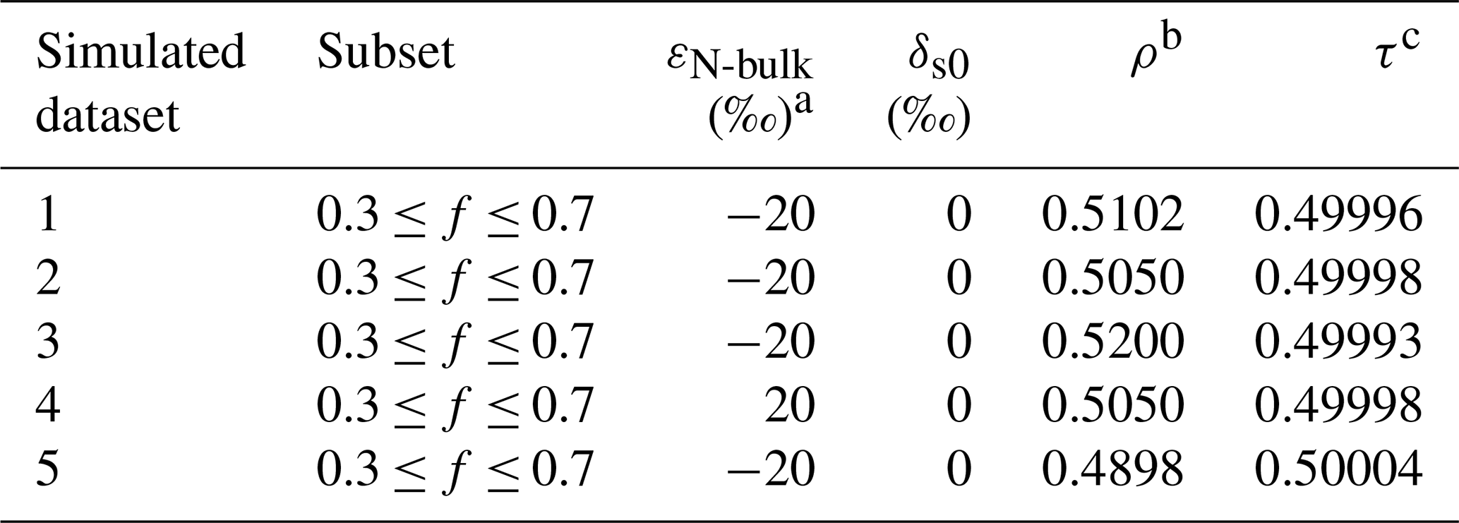
^a Note that an ε value of −20 ‰ corresponds to a KIE of 1.0204 and an ε value of +20 ‰ corresponds to a KIE of 0.9804. ^b Parameter introduced in the Expanded Rayleigh model (Eq. 23): ρ = ¹⁵N${}^{\mathit{\alpha }}{/}^{\mathrm{15}}$N^bulk. ^c Parameter introduced in the Expanded Rayleigh model (Eq. 24): τ = ¹⁴N${}^{\mathit{\alpha }}{/}^{\mathrm{14}}$N^bulk. τ was calculated for each value of f; the average value of τ is listed.

Figure 1 Simulated δ¹⁵N values for N₂O synthesis in a closed system with different combinations of KIE ¹⁵N^α and KIE ¹⁵N^β. δ¹⁵N values of remaining substrate (δ¹⁵N^s) and accumulated product (N₂O) (δ¹⁵N^bulk, δ¹⁵N^α, and δ¹⁵N^β) are plotted as a function of the fraction of substrate reduced (1−f) with reactions progressing from left to right. Values of δ¹⁵N^bulk and δ¹⁵N^s were calculated using Eq. (2) or Eq. (18) (Mariotti's approximation of the Rayleigh equation; Mariotti et al., 1981), where ε¹⁵N^bulk is set to −20 ‰ (Datasets 1–3 and 5) or +20 ‰ (Dataset 4) and the initial δ¹⁵N^s value (δ¹⁵N^s0) is set to 0 ‰. Values of δ¹⁵N^α and δ¹⁵N^β were calculated using Eqs. (27) and (28). For Datasets 1 and 5, either ε¹⁵N^α or ε¹⁵N^β was set to 0 ‰ (no isotope effect, KIE = 1), and the corresponding value of ρ was back-calculated (see the Supplement for details). For Datasets 2–4, values of δ¹⁵N^α and δ¹⁵N^β were calculated using pre-determined values of ρ that were less than (Datasets 2 and 4) or greater than (Dataset 3) the value of ρ from Dataset 1. See Table 3 for the KIE values for each simulation.

2.5 Nonlinear expansion of the Rayleigh model

Simulated δ¹⁵N^α and δ¹⁵N^β values were calculated based on the assumption that, like the fractionation factor for bulk N, the fractionation factors for the individual N^α and N^β atoms are constant (see Assumption 6 above). To relate α_N−α and α_N−β to α_N-bulk, we define the fraction of instantaneously converted ¹⁵N^bulk (¹⁵N^bulk,i) that is incorporated into the α position as ρ (Eq. 19).

$$\begin{array}{}\text{(19)}& \mathit{\rho }={\displaystyle \frac{{}^{\mathrm{15}}{\mathrm{N}}^{\mathit{\alpha },i}}{{}^{\mathrm{15}}{\mathrm{N}}^{\mathrm{bulk},i}}}\end{array}$$

Similarly, we define the fraction of instantaneously converted ¹⁴N (¹⁴N^bulk,i) that goes to the α position as τ (Eq. 20).

$$\begin{array}{}\text{(20)}& \mathit{\tau }={\displaystyle \frac{{}^{\mathrm{14}}{\mathrm{N}}^{\mathit{\alpha },i}}{{}^{\mathrm{14}}{\mathrm{N}}^{\mathrm{bulk},i}}}\end{array}$$

In keeping with the premise that α_N−α and α_N−β are constant, we assume a priori that ρ and τ are constant. Thus, the equation for α_N−α may be written in terms of ρ, τ, and α_N-bulk.

$$\begin{array}{}\text{(21)}& {\mathit{\alpha }}_{\mathrm{N}-\mathit{\alpha }}={\displaystyle \frac{\frac{\mathit{\rho }{\cdot }^{\mathrm{15}}{\mathrm{N}}^{\mathrm{bulk},i}}{\mathit{\tau }{\cdot }^{\mathrm{14}}{\mathrm{N}}^{\mathrm{bulk},i}}}{\frac{{}^{\mathrm{15}}{N}^{\mathrm{s}}}{{}^{\mathrm{14}}{\mathrm{N}}^{\mathrm{s}}}}}={\displaystyle \frac{\mathit{\rho }}{\mathit{\tau }}}\cdot {\mathit{\alpha }}_{\text{N-bulk}}\end{array}$$

In the absence of side reactions, ¹⁵N^bulk,i must be equal to the sum of ¹⁵N^α,i and ¹⁵N^β,i. Similarly, ¹⁴N^bulk,i must be equal to the sum of ¹⁴N^α,i and ¹⁴N^β,i. Thus, the equation for α_N−β may also be written in terms of ρ, τ, and α_N-bulk.

$$\begin{array}{}\text{(22)}& {\mathit{\alpha }}_{\mathrm{N}-\mathit{\beta }}={\displaystyle \frac{\frac{\left(\mathrm{1}-\mathit{\rho }\right){\cdot }^{\mathrm{15}}{\mathrm{N}}^{\mathrm{bulk},i}}{\left(\mathrm{1}-\mathit{\tau }\right){\cdot }^{\mathrm{14}}{\mathrm{N}}^{\mathrm{bulk},i}}}{\frac{{}^{\mathrm{15}}{N}_{\mathrm{s}}}{{}^{\mathrm{14}}{\mathrm{N}}_{\mathrm{s}}}}}={\displaystyle \frac{\mathrm{1}-\mathit{\rho }}{\mathrm{1}-\mathit{\tau }}}\cdot {\mathit{\alpha }}_{\text{N-bulk}}\end{array}$$

Equations (21) and (22) form the basis for the Expanded Rayleigh model.

To simulate δ¹⁵N^α and δ¹⁵N^β values and determine the corresponding fractionation factors, ρ and τ must be related to accumulated isotope ratios, R_α and R_β. Although ρ is formally defined in Eq. (19) as the fraction of instantaneously converted ¹⁵N apportioned to the α position, ρ can also be written in terms of accumulated ¹⁵N values as long as ρ is constant.

$$\begin{array}{}\text{(23)}& \mathit{\rho }={\displaystyle \frac{{}^{\mathrm{15}}{\mathrm{N}}^{\mathit{\alpha }}}{{}^{\mathrm{15}}{\mathrm{N}}^{\mathrm{bulk}}}}\end{array}$$

Similarly, as long as τ is constant, τ may be written in terms of accumulated ¹⁴N values.

$$\begin{array}{}\text{(24)}& \mathit{\tau }={\displaystyle \frac{{}^{\mathrm{14}}{\mathrm{N}}^{\mathit{\alpha }}}{{}^{\mathrm{14}}{\mathrm{N}}^{\mathrm{bulk}}}}\end{array}$$

Using the definition of ρ from Eq. (23), R_α can be written in terms of ρ by substituting ¹⁵N^α with ρ⋅¹⁵N^bulk and replacing ¹⁴N^α with 0.5 ⋅ (N^bulk) - ¹⁵N^α (Eq. 25).

$$\begin{array}{}\text{(25)}& R_{\mathit{\alpha }}={\displaystyle \frac{{}^{\mathrm{15}}{\mathrm{N}}^{\mathit{\alpha }}}{{}^{\mathrm{14}}{\mathrm{N}}^{\mathit{\alpha }}}}={\displaystyle \frac{\mathit{\rho }{\cdot }^{\mathrm{15}}{\mathrm{N}}^{\mathrm{bulk}}}{\mathrm{0.5}\cdot {\mathrm{N}}^{\mathrm{bulk}}-\mathit{\rho }{\cdot }^{\mathrm{15}}{\mathrm{N}}^{\mathrm{bulk}}}}\end{array}$$

The same approach can be used to define R_β in terms of ρ (Eq. 26).

$$\begin{array}{}\text{(26)}& R_{\mathit{\beta }}={\displaystyle \frac{{}^{\mathrm{15}}{\mathrm{N}}^{\mathit{\beta }}}{{}^{\mathrm{14}}{\mathrm{N}}^{\mathit{\beta }}}}={\displaystyle \frac{(\mathrm{1}-\mathit{\rho }){\cdot }^{\mathrm{15}}{\mathrm{N}}^{\mathrm{bulk}}}{\mathrm{0.5}\cdot {\mathrm{N}}^{\mathrm{bulk}}-(\mathrm{1}-\mathit{\rho }){\cdot }^{\mathrm{15}}{\mathrm{N}}^{\mathrm{bulk}}}}\end{array}$$

The term 0.5 ⋅ N^bulk is equal to moles of N₂O (Eq. 7), and ¹⁵N^bulk can be calculated for any value of f using N^bulk and δ¹⁵N^bulk (see the Supplement). Equations (25) and (26) can be converted to δ notation as follows (see Eq. 6).

$$\begin{array}{}\text{(27)}& {\displaystyle }{\mathit{\delta }}^{\mathrm{15}}{\mathrm{N}}^{\mathit{\alpha }}=\left({\displaystyle \frac{\mathit{\rho }{\cdot }^{\mathrm{15}}{\mathrm{N}}^{\mathrm{bulk}}}{(\mathrm{0.5}\cdot {\mathrm{N}}^{\mathrm{bulk}}-\mathit{\rho }{\cdot }^{\mathrm{15}}{\mathrm{N}}^{\mathrm{bulk}})\cdot R_{\mathrm{standard}}}}-\mathrm{1}\right)\cdot \mathrm{1000}\text{(28)}& {\displaystyle }{\mathit{\delta }}^{\mathrm{15}}{\mathrm{N}}^{\mathit{\beta }}=\left({\displaystyle \frac{\left(\mathrm{1}-\mathit{\rho }\right){\cdot }^{\mathrm{15}}{\mathrm{N}}^{\mathrm{bulk}}}{(\mathrm{0.5}\cdot {\mathrm{N}}^{\mathrm{bulk}}-(\mathrm{1}-\mathit{\rho }\left){\cdot }^{\mathrm{15}}{\mathrm{N}}^{\mathrm{bulk}}\right)\cdot {\mathrm{R}}_{\mathrm{standard}}}}-\mathrm{1}\right)\cdot \mathrm{1000}\end{array}$$

Equations (27) and (28) can be used to determine δ¹⁵N^α and δ¹⁵N^β based on δ¹⁵N^bulk as long as ρ is constant and δ¹⁵N^bulk can be approximated as the average of δ¹⁵N^α and δ¹⁵N^β (see Eq. 15 and Table S3).

2.6 Simulation of error-free δ¹⁵N^α and δ¹⁵N^β values

Idealized, error-free δ¹⁵N^α and δ¹⁵N^β values (shown in Fig. 1) were simulated for the values of ρ listed in Table 1 by calculating δ¹⁵N^α and δ¹⁵N^β using Eqs. (27) and (28) (Tables S4–8). As outlined in Table 1, five different scenarios with different combinations of isotope effects (none, normal, or inverse) for the α and β nitrogen atoms of N₂O were simulated. For Datasets 1 and 5, either ε¹⁵N^α or ε¹⁵N^β was set to 0 ‰ (no isotope effect, KIE = 1), and the corresponding values of ρ and τ were back-calculated (see the Supplement for details). The remaining values of ρ were chosen to produce datasets with the different combinations of normal and/or inverse isotope effects (Datasets 2–4). The ρ values tested (0.4898–0.5200) are all close enough to 0.5 such that the average of δ¹⁵N^α and δ¹⁵N^β is approximately equal to δ¹⁵N^bulk (Table S3). In all cases, discrepancies between δ¹⁵N^bulk values calculated using Eq. (2) and δ¹⁵N^bulk values calculated by averaging δ¹⁵N^α and δ¹⁵N^β (Eq. 15) are well below the typical analytical error of 0.5 ‰–0.7 ‰ (Yang et al., 2014).

2.7 Determination of ρ and τ for the Expanded Rayleigh model

To determine α_N−α and α_N−β using Eqs. (21) and (22), ρ and τ must be calculated using values that can be measured experimentally (see Fig. 2 for the general workflow for using the Expanded Rayleigh model to determine α_N−α and α_N−β). Because the abundance of ¹⁴N is so much greater than that of ¹⁵N, variations in ¹⁵N apportionment between N^α and N^β are negligible when determining the fraction of ¹⁴N^bulk at the α position (i.e., τ). For enzyme-catalyzed N₂O synthesis with substrate at or near the natural abundance of ¹⁵N, we have found that τ is always 0.5000 (see the analysis of data from Sutka et al., 2006, and Yang et al., 2014, below). For the purposes of testing our new Expanded Rayleigh model, we calculated more precise values of τ. To do this, τ was calculated for each value of f using Eq. (24), and the average τ value for each dataset was used to calculate fractionation factors.

To determine ρ using values that can be measured experimentally, Eq. (15) is rewritten so that ρ is the only unknown parameter. This can be accomplished by replacing δ¹⁵N^α with the equivalent term from Eq. (27), producing Eq. (29), a nonlinear equation we have named nonlinear model 1.

$$\begin{array}{}\text{(29)}& \begin{array}{rl}{\mathit{\delta }}^{\mathrm{15}}{\mathrm{N}}^{\mathrm{bulk}}& ={\displaystyle \frac{\mathrm{1}}{\mathrm{2}}}\cdot [\left({\displaystyle \frac{\mathit{\rho }{\cdot }^{\mathrm{15}}{\mathrm{N}}^{\mathrm{bulk}}}{\left(\mathrm{0.5}\cdot {\mathrm{N}}^{\mathrm{bulk}}-\mathit{\rho }{\cdot }^{\mathrm{15}}{\mathrm{N}}^{\mathrm{bulk}}\right)\cdot R_{\mathrm{standard}}}}-\mathrm{1}\right)\\ & \cdot \mathrm{1000}+{\mathit{\delta }}^{\mathrm{15}}{\mathrm{N}}^{\mathit{\beta }}]\end{array}\end{array}$$

Alternatively, δ¹⁵N^β could be replaced with a term that includes ρ (Eq. 28), producing Eq. (30) (nonlinear model 2).

$$\begin{array}{}\text{(30)}& \begin{array}{rl}{\mathit{\delta }}^{\mathrm{15}}{\mathrm{N}}^{\mathrm{bulk}}& ={\displaystyle \frac{\mathrm{1}}{\mathrm{2}}}\cdot [{\mathit{\delta }}^{\mathrm{15}}{\mathrm{N}}^{\mathit{\alpha }}\\ & +\left({\displaystyle \frac{\left(\mathrm{1}-\mathit{\rho }\right){\cdot }^{\mathrm{15}}{\mathrm{N}}^{\mathrm{bulk}}}{\left(\mathrm{0.5}\cdot {\mathrm{N}}^{\mathrm{bulk}}-(\mathrm{1}-\mathit{\rho }){\cdot }^{\mathrm{15}}{\mathrm{N}}^{\mathrm{bulk}}\right)\cdot R_{\mathrm{standard}}}}-\mathrm{1}\right)\\ & \cdot \mathrm{1000}]\end{array}\end{array}$$

Both nonlinear models were used to find the optimal value of ρ via nonlinear least-squares regression for each of our simulated datasets.

2.8 Generation of datasets with simulated error

To mimic experimental error, 1000 simulated datasets were generated from each error-free dataset by adding random error to N^s, δ¹⁵N^bulk, and δ¹⁵N^α using a modified version of the procedure outlined by Scott and colleagues (Scott et al., 2004). Error was propagated to f by recalculating f using the N^s values with error added (f = N^s / N^s0). Similarly, error was propagated to δ¹⁵N^β by recalculating δ¹⁵N^β using δ¹⁵N^bulk and δ¹⁵N^α values with error added (Eq. 15). For each simulation, fractionation factors and KIE values were calculated using the standard Rayleigh model and the Expanded Rayleigh model (versions 1 and 2), and the KIE values from each set of 1000 simulations were averaged. Three “levels” of error (low, medium, and high) and three types of skewness (none, left-skewed, and right-skewed; see below) were used for a total of nine conditions (Table 2; Figs. 3 and S1–4). For simulations with low error, the standard deviation of each randomly generated error term was set to the level of error expected in a typical experiment (Table 2). The standard deviation of N^s values was set to 1.5 % of N^s0 (the maximum value of N^s), which corresponds to the estimated level of error in gas volume measurements (see the Supplement). The standard deviations of δ¹⁵N^bulk and δ¹⁵N^α were set to 0.5 ‰ and 0.7 ‰, respectively, which correspond to standard deviations typical for isotopic analysis of N₂O via isotope ratio mass spectrometry (IRMS) (Yang et al., 2014). To further test the robustness of the linear and nonlinear models, medium- and high-level error terms were generated by multiplying the low-level error terms for N^s, δ¹⁵N^bulk, and δ¹⁵N^α by the appropriate factor (Table 2). The multiplication factors for medium- and high-level error were chosen so that the average R² values produced by linear regression of δ¹⁵N^bulk against [$-f\ln f/(\mathrm{1}-f)$] were approximately 0.7 and 0.4, respectively. Similar R² values have been observed for standard Rayleigh linear regression plots for N₂O biosynthesis (e.g., Yang et al., 2014; Figs. S2–4).

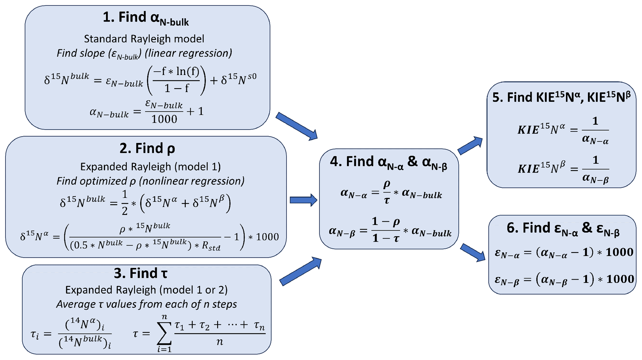
Figure 2 General workflow for using the Expanded Rayleigh model to determine fractionation factors (α) and kinetic isotope effects (KIEs) for the individual N atoms (N^α and N^β) in N₂O. To determine the fractionation factors for the α and β atoms in N₂O (α_N−α and α_N−β), three separate values must be calculated. (1) The fractionation factor for bulk N (α_N-bulk) is determined by finding the slope (ε_N-bulk) of a standard Rayleigh plot where y = [$-f\ln f/(\mathrm{1}-f)$] and x=δ¹⁵N^bulk and converting ε_N-bulk to α_N-bulk as has been previously described (Mariotti et al., 1981). (2) Nonlinear modeling is used to determine the optimal value of ρ (the fraction of ¹⁵N^bulk at the α position). For Expanded Rayleigh model 1 (shown here), δ¹⁵N^α is replaced in the top equation with an equivalent expression that includes ρ (bottom equation) to generate the model used for nonlinear least-squares regression (Eq. 29). For Expanded Rayleigh model 2, δ¹⁵N^β is substituted, producing Eq. (30) (not shown). (3) The value of τ (the fraction of ¹⁴N^bulk at the α position) is determined by dividing ¹⁴N^α by ¹⁴N^bulk for each step of the reaction and averaging the results. (4) Finally, α_N-bulk, ρ, and τ are used to calculate α_N−α and α_N−β. (5–6) These individual fractionation factors can be converted to the corresponding KIE values (Eq. 10) or ε values (Eq. 1).

Figure 3 Example simulations derived from Dataset 1 with varying levels of error and types of skewness. Each panel shows a single dataset (representative of 1000 simulated datasets) consisting of three replicates with five time points each. All simulations were derived from Dataset 1 (δ¹⁵N^s0= 0 ‰, ε_N-bulk= −20 ‰ (KIE ¹⁵N^bulk= 1.0204), KIE ¹⁵N^α= 1.0000, and KIE ¹⁵N^β= 1.0417). Each level of error and type of skewness is described in Table 2. Example graphs derived from Datasets 2–4 are shown in Figs. S1–4.

For each level of error, three sets of 1000 simulations with different types of skewness (no skew, left-skewed, or right-skewed) were performed to mimic types of skewness that might be observed in experimental data. For example, if N₂O leaks from a sample bottle prior to analysis, the quantity of N₂O produced will be underestimated, and the corresponding values of N^s and f will be overestimated. Additionally, since light isotopes have a higher rate of both diffusion and effusion, values of δ¹⁵N^bulk, δ¹⁵N^α, and δ¹⁵N^β will be overestimated. This scenario is represented by simulations where the random error values added to N^s, δ¹⁵N^bulk, and δ¹⁵N^α were derived from left-skewed distributions. Skewness classifications were then assigned based on the skewness of the residuals for the standard Rayleigh model where the dependent variable (y) is δ¹⁵N^bulk (Table 2). Simulations with residuals between −0.5 and 0.5 (inclusive) were designated “no skew,” meaning the distribution of these residuals did not differ significantly from the normal distribution. Simulations where standard Rayleigh residuals had a skewness value less than −0.5 were designated “left-skewed” (i.e., left-tailed distribution), and simulations where skewness was greater than 0.5 were designated “right-skewed” (i.e., right-tailed distribution).

Table 2 Standard deviation and skewness of random error added to simulated N^s, δ¹⁵N^bulk, and δ¹⁵N^α values.

^a “Level of error” refers to the standard deviations of N^s (nmol of remaining substrate), δ¹⁵N^bulk, and δ¹⁵N^a. ^b Skewness of the residuals for the standard Rayleigh model (linear regression of δ¹⁵N^bulk against [$-f\ln f/(\mathrm{1}-f)$]). ^c N^s0 refers to nanomoles (nmol) of substrate at time 0 (i.e., the maximum amount of substrate). N^s0 was set to 10 000 nmol in all simulations.

Table 3 KIE values for N^bulk, N^α, and N^β calculated directly from simulation input values (Actual) or from the standard Rayleigh model or Expanded Rayleigh model applied to error-free simulated datasets.

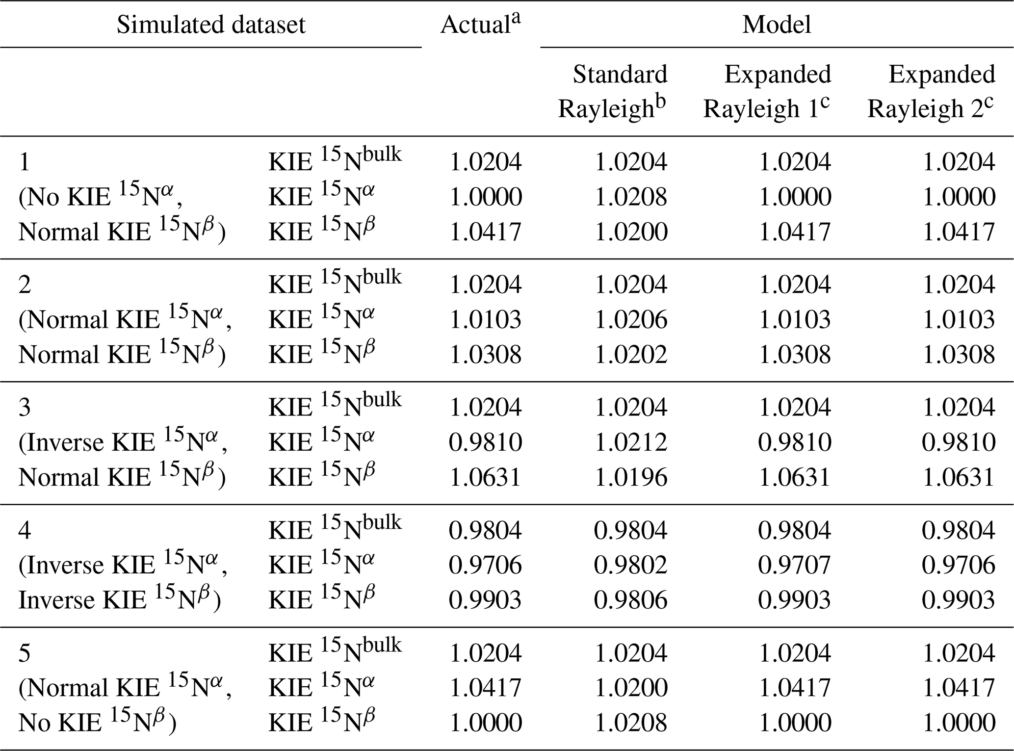
^a Actual values were calculated directly from the input values used to generate the dataset. ^b KIE values were calculated from ε_N-bulk, ε_N−α, or ε_N−β values obtained via linear regression of δ¹⁵N^bulk, δ¹⁵N^α, or δ¹⁵N^β against [$-f\ln f/(\mathrm{1}-f)$] (see Eq. 2). ^c For the Expanded Rayleigh model, α_N-bulk was determined with the standard Rayleigh approach, ρ was determined via nonlinear regression (nonlinear model 1 or 2, Eq. 29 or Eq. 30), and τ was determined by averaging ¹⁴N${}^{\mathit{\alpha }}{/}^{\mathrm{14}}$N^bulk for every step of the reaction.

To assess the accuracy of each model under different circumstances, average KIE values and standard deviations were calculated for each set of 1000 simulations with error. The absolute relative difference of each average KIE was calculated using Eq. (31):

$$\begin{array}{}\text{(31)}& \text{absolute relative difference}=\mathrm{|}{\displaystyle \frac{\text{estimate}-\text{actual}}{\text{actual}}}\mathrm{|},\end{array}$$

where the estimate is the average KIE and actual values were calculated directly from the input values for simulations without error (see Table 3). Lower absolute relative difference values indicate higher accuracy. Goodness of fit was assessed for the (linear) standard Rayleigh model and nonlinear models 1 and 2 by calculating the average root mean square error (RMSE) for each set of 1000 simulations. For each simulation, p values for ε_N-bulk and ρ (coefficients extracted from the (linear) standard Rayleigh model and nonlinear model 1 or 2, respectively) were determined using the one-sample t test (two-sided) (Baty et al., 2015; Ritz and Streibig, 2008; Kalpiæ et al., 2011). The null hypothesis used to calculate these p values is that there is no kinetic isotope effect. For the linear model, this means that the null hypothesis is ε_N-bulk= 0 (KIE ¹⁵N^bulk= 1). For the nonlinear models, the null hypothesis is that ρ= 0.5 (KIE ¹⁵N^α= 1 and KIE ¹⁵N^β= 1).

2.9 Analysis of previously published experimental data

The standard and Expanded Rayleigh models were applied to published data on N₂O produced from NH₂OH by Methylosinus trichosporium (ATCC 49243) (Sutka et al., 2006). We calculated values of f, δ¹⁵N^α, and δ¹⁵N^β using the N₂O concentrations, δ¹⁵N^bulk values, and site preference (SP) values from replicate B measured by Sutka et al. (see Table S14 for original data and our calculated values and Fig. 4 for a graphical representation of these data). SP is defined as the difference between δ¹⁵N^α and δ¹⁵N^β.

$$\begin{array}{}\text{(32)}& \mathrm{SP}={\mathit{\delta }}^{\mathrm{15}}{\mathrm{N}}^{\mathit{\alpha }}-{\mathit{\delta }}^{\mathrm{15}}{\mathrm{N}}^{\mathit{\beta }}\end{array}$$

The data for replicate B were chosen because these data had a range of f values large enough for ε_N-bulk to be determined via the standard Rayleigh method (linear regression of δ¹⁵N^bulk against [$-f\ln f/(\mathrm{1}-f)$]). See the Supplement for details.

Figure 4 Experimentally measured δ¹⁵N values for N₂O synthesis from NH₂OH in a pure culture of Methylosinus trichosporium (data modified from Sutka et al., 2006). Data previously reported for M. trichosporium (Methylocystis sp.) replicate B (Sutka et al., 2006). δ¹⁵N values of accumulated product (N₂O) (δ¹⁵N^bulk, δ¹⁵N^α, and δ¹⁵N^β) are plotted as a function of the fraction of substrate consumed (1−f) with the reaction progressing from left to right. We back-calculated values of f, δ¹⁵N^α, and δ¹⁵N^β using the reported N₂O concentrations, δ¹⁵N^bulk values, and SP values. The initial measured δ¹⁵N value of NH₂OH (δ¹⁵N^s0), −2.3 ‰, is shown at f = 1.

We also applied the standard and Expanded Rayleigh models to previously published isotopic data on N₂O production from purified Histoplasma capsulatum (fungal) P450 NOR (Fig. 5 and Table S16) (Yang et al., 2014). Because this dataset covered a wide range of f values (f = 0.42-0.87) and δ¹⁵N^bulk varied linearly with [$-f\ln f/(\mathrm{1}-f)$], we used the standard Rayleigh model (Eq. 2) to determine ε_N-bulk via linear regression of δ¹⁵N^bulk against [$-f\ln f/(\mathrm{1}-f)$]. ε_N-bulk was determined for each of three independent biological replicates (13 observations per replicate), and the results were averaged. Similarly, to determine standard Rayleigh values of ε_N−α and ε_N−β, we performed linear regression of δ¹⁵N^α or δ¹⁵N^β against [$-f\ln f/(\mathrm{1}-f)$] for each independent replicate and averaged the results.

Figure 5 Experimentally measured product δ¹⁵N values and calculated δ¹⁵N^s0 values for N₂O synthesis from NO by purified H. capsulatum P450 NOR. Adapted with permission from Yang et al. (2014). Copyright 2014 American Chemical Society. Data previously reported for H. capsulatum (fungal) P450 NOR replicates A–C (Yang et al., 2014). δ¹⁵N values of accumulated product (N₂O) (δ¹⁵N^bulk, δ¹⁵N^α, and δ¹⁵N^β) are plotted as a function of the fraction of substrate reduced (1−f) with the reaction progressing from left to right. We back-calculated δ¹⁵N^s0 for each replicate by finding the intercept of the corresponding standard Rayleigh plot (Eq. 2) where x = [$-f\ln f/(\mathrm{1}-f)$] and y=δ¹⁵N^bulk.

To apply the Expanded Rayleigh model to the isotopic data on N₂O production by P450 NOR, we used a modified procedure because, in this case, ρ and τ vary linearly with [$-f\ln f/(\mathrm{1}-f)$]. Using nonlinear regression to determine ρ yields a value of ρ in between the more extreme values of ρ observed at the start and end of the reaction and does not represent the data from the overall reaction very well. Therefore, instead of using nonlinear model 1 (Eq. 29) or model 2 (Eq. 30) to determine ρ using data from the entire reaction, we calculated ρ for each individual time point (i.e., each individual value of f) using Eq. (23). Similarly, τ was calculated for each individual observation using Eq. (24). These individual ρ and τ values were then used to calculate α_N−α (Eq. 21) and α_N−β (Eq. 22) values for each value of f, which were then converted to KIE values using Eq. (10). This approach yielded KIE values that increased (KIE ¹⁵N^α) or decreased (KIE ¹⁵N^β) as the reaction progressed. To estimate the range of position-specific KIEs produced by the Expanded Rayleigh model, individual KIE ¹⁵N^α and KIE ¹⁵N^β values representing the early part of the reaction (f = 0.8 ± 0.03) or the latter part of the reaction (late reaction, f = 0.5 ± 0.03) were averaged (Tables 6 and S17).

2.10 Modeling, statistical analysis, and figures

Modeling and statistical analyses of simulated and experimental δ values were performed with R statistical software (R Core Team, 2022), and figures were produced with ggplot2 (Wickham, 2016). To determine ρ for the Expanded Rayleigh model, nonlinear least-squares regression was performed as previously described (Baty et al., 2015) using a starting ρ value of 0.5.

For datasets with simulated error, random numbers representing simulated error were generated using the rsn function from the skew-normal distribution package (Azzalini, 2023), and skewness was calculated with the moments package (Komsta and Novomestky, 2022). In the moments package, skewness is defined as $(\mathrm{1}/n)\cdot \mathrm{\Sigma }\left(\right(x-\stackrel{\mathrm{‾}}{x})/s{)}^{\mathrm{3}}$, where n is the sample size, $\stackrel{\mathrm{‾}}{x}$ is the sample mean, and s is the sample standard deviation (Hippel, 2011).

For previously published experimental data, a linear model was used to determine if SP, ρ, or τ varied as a function of [$-f\ln f/(\mathrm{1}-f)$].

3 Results

3.1 Error-free simulations

To demonstrate that the standard Rayleigh model produces inaccurate results for the individual nitrogen atoms in N₂O, idealized, error-free datasets were simulated representing different scenarios with varying combinations of KIEs for N^α and N^β (Fig. 1 and Table 1). Because these data were simulated assuming that the fractions of ¹⁵N and ¹⁴N apportioned to each position remain constant (i.e., constant ρ and τ), the distance between δ¹⁵N^α and δ¹⁵N^β over the course of each reaction is constant, and the rates of change in δ¹⁵N^α, δ¹⁵N^β, and δ¹⁵N^bulk with respect to reaction progress (1−f) are essentially equal (Fig. 1). Thus, when the standard Rayleigh model (Eq. 2) is applied to each dataset, the slopes (ε) of δ¹⁵N^α, δ¹⁵N^β, and δ¹⁵N^bulk against [$-f\ln f/(\mathrm{1}-f)$] for each dataset are all approximately equal, as are the corresponding KIE ¹⁵N^bulk, KIE ¹⁵N^α, and KIE ¹⁵N^β values (Table 3). While the standard Rayleigh KIE ¹⁵N^bulk values match the actual KIE ¹⁵N^bulk values, the KIE ¹⁵N^α and KIE ¹⁵N^β values determined using the standard Rayleigh approach differ significantly from the actual KIEs calculated from simulation input values (Table 3). In each of the five simulated reactions (Datasets 1–5), the isotopic preference for N^α differs from that of N^β, which can be verified visually by noting that the δ¹⁵N^α values are significantly different than the δ¹⁵N^β values throughout each reaction (Fig. 1). However, in all five cases, the standard Rayleigh model produces KIE values for N^α and N^β that are approximately equal, highlighting the fact that the standard Rayleigh model inaccurately quantifies ¹⁵N apportionment between N^α and N^β. (If KIE ¹⁵N^α were equal to KIE ¹⁵N^β, the curves for δ¹⁵N^α, δ¹⁵N^β, and δ¹⁵N^bulk shown in Fig. 1 would all be on top of each other.)

The inadequacies of the standard Rayleigh model are most evident when N^α and N^β have opposing kinetic isotope effects, i.e., scenarios where there is an inverse isotope effect at one position and a normal isotope effect at the other position (Dataset 3), or when only one position has a nonzero fractionation factor (Datasets 1 and 5). In these cases, the standard Rayleigh model fails to predict the correct type of isotope effect for one of the nitrogen atoms. For example, Dataset 1 represents a scenario where there is no isotopic preference at the α position, meaning instantaneous δ¹⁵N^α (δ¹⁵N^αi) is always equal to δ¹⁵N^s, which can be verified visually by noting that accumulated δ¹⁵N^α≈δ¹⁵N^s at the start of the reaction (Fig. 1). Under these circumstances, KIE ¹⁵N^α is equal to 1.0000. However, the standard Rayleigh model predicts a much higher KIE ¹⁵N^α value (1.0208), incorrectly indicating that there is a reasonably strong, normal KIE at the α position. The standard Rayleigh KIE ¹⁵N^β value calculated for Dataset 1 is also too low (1.0200 instead of 1.0417), underestimating the preference for ¹⁴N at the β position. Similarly misleading results are produced for Dataset 5, where there is no isotope effect for N^β, but the standard Rayleigh model predicts a normal isotope effect at this position. Along the same lines, the standard Rayleigh KIE values for Dataset 3 incorrectly indicate that both N^α and N^β have normal isotope effects when, in this case, N^α actually has an inverse isotope effect. Thus, even for a simulated dataset with no experimental error, the standard Rayleigh model produces results that are quantitatively – and sometimes qualitatively – incorrect.

The standard Rayleigh model produces inaccurate results for the individual N atoms in N₂O because the changes in δ¹⁵N^α depend on both KIE ¹⁵N^α and KIE ¹⁵N^β, as do changes in δ¹⁵N^β. Linear regression of standard Rayleigh plots for δ¹⁵N^α or δ¹⁵N^β fails to capture this nuance. To address this issue, we developed the Expanded Rayleigh model that introduces two new parameters, ρ and τ, to define how ¹⁵N^bulk and ¹⁴N^bulk, respectively, are apportioned between N^α and N^β. Fractionation factors for N^α and N^β are determined by combining α_N-bulk, ρ, and τ (Eqs. 21 and 22). For experiments conducted at the natural abundance of ¹⁵N, the value of τ, which is equal to ¹⁴N^α/¹⁴N^bulk, should always be quite close to 0.5, as discussed above. Indeed, each simulated reaction step has a mean value of τ equal to 0.500 for Datasets 1–5 (Tables S9–13), so the average value of ¹⁴N${}^{\mathit{\alpha }}{/}^{\mathrm{14}}$N^bulk was used to calculate α_N−α and α_N−β. To determine the value of ρ that fits the entire dataset as accurately as possible, we performed nonlinear least-squares regression using the formula shown in Eq. (29) (nonlinear model 1) or Eq. (30) (nonlinear model 2). For error-free Datasets 1–5, nonlinear least-squares regression with either nonlinear model correctly predicted ρ. Combining these ρ and τ values with α_N-bulk values derived from the standard Rayleigh equation yields KIE ¹⁵N^α and KIE ¹⁵N^β values that are identical to the expected values out to three or four decimal places (Table 3). Thus, unlike the standard Rayleigh approach, the Expanded Rayleigh model successfully recapitulates the kinetic isotope effects for N^α and N^β in an error-free dataset.

Table 4 Precision and accuracy of values calculated with Expanded Rayleigh model 1 using simulated datasets derived from Dataset 1 (no isotope effect for N^α, normal isotope effect for N^β). n/a – not applicable.

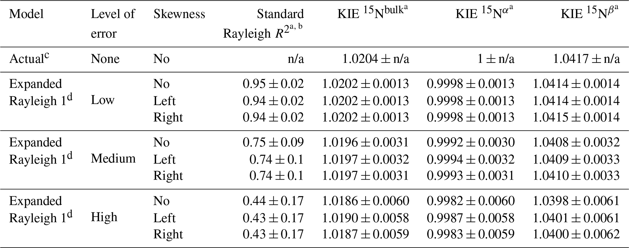
^a Average value ± standard deviation calculated from 1000 values generated from 1000 simulated datasets. ^b Average R² value for linear regression of δ¹⁵N^bulk against [$-f\ln f/(\mathrm{1}-f)$] (using Eq. 2, the standard Rayleigh equation). ^c Actual values were calculated directly from the input values used to generate the dataset. ^d For Expanded Rayleigh model 1, α_N-bulk was determined with the standard Rayleigh approach, ρ was determined via nonlinear regression (nonlinear model 1, Eq. 29), and τ was determined by averaging ¹⁴N${}^{\mathit{\alpha }}{/}^{\mathrm{14}}$N^bulk for every step of the reaction (Eq. 24). The results for Expanded Rayleigh model 2 (Table S9) are very similar.

3.2 Application of the Expanded Rayleigh model to simulations with error

To test the robustness of the Expanded Rayleigh model, we applied this model to simulated data with error at varying levels of size and skewness (Table 2; Figs. 3 and S1–4) and averaged the results from 1000 simulations for each error category (Tables 4 and S9–13). These results indicate that at a low level of error (the level of error expected for a typical experiment), the KIE values produced by the Expanded Rayleigh model are quite accurate (absolute difference relative to true values is 0.001, or 0.1 %, see Eq. 31), regardless of the skewness of the standard Rayleigh model residuals (Figs. 6 and S5–8). The standard deviations for each average KIE ¹⁵N^bulk, KIE ¹⁵N^α, or KIE ¹⁵N^β value (0.0013–0.0014) are also similar to standard error values from typical experiments (∼ 0.0004–0.0021) (Tables 5 and 6) (Sutka et al., 2006; Yang et al., 2014). As the absolute value of the simulated error increases, the average KIE values become less accurate, and the corresponding standard deviations increase. Nonetheless, even at the highest level of error, the maximum absolute relative difference of average KIE values is 0.005 (0.5 % difference), and the range of values covered by average KIE ± standard deviation includes the actual KIE value. Thus, the Expanded Rayleigh model provides a robust method for determining KIE values even when the datasets have a high level of error or skewness.

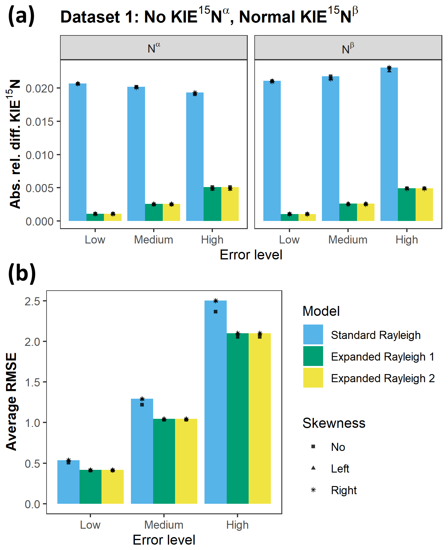
Figure 6 Comparison of the accuracy and goodness of fit of the standard Rayleigh model and Expanded Rayleigh models 1 and 2. (a) Comparison of the accuracy of KIE ¹⁵N^α and KIE ¹⁵N^β values. For each model, the absolute relative difference for KIE ¹⁵N^α and KIE ¹⁵N^β values (average for 1000 simulated datasets derived from Dataset 1) is shown. Actual values for Dataset 1: δ¹⁵N^s0= 0 ‰, ε_N-bulk= −20 ‰ (KIE ¹⁵N^bulk= 1.0204), KIE ¹⁵N^α= 1.0000, and KIE ¹⁵N^β= 1.0417. Absolute relative difference (Eq. 31) is the absolute value of the difference between the estimated value and actual value divided by the actual value (|(estimate – actual)/actual|). (b) Comparison of the average RMSE values for each set of 1000 simulated datasets derived from Dataset 1. Both the standard Rayleigh model and the Expanded Rayleigh model (1 and 2) use δ¹⁵N^bulk as the dependent variable, so average RMSE values can be compared directly. Lower RMSE values indicate a better goodness of fit. At each error level (low, medium, and high), the absolute relative difference value (a) or average RMSE (b) is depicted with a symbol that represents skewness type as shown in the legend. Note that in most cases these symbols overlap.

In contrast to the Expanded Rayleigh model, the KIE ¹⁵N^α and KIE ¹⁵N^β values determined for simulations with error using the standard Rayleigh model alone are much less accurate (Figs. 6 and S5–8). For all simulations derived from Datasets 1–5 at all levels of error and types of skewness, the absolute relative differences of average standard Rayleigh KIE ¹⁵N^α and KIE ¹⁵N^β values ranged from 0.01–0.04 (1 %–4 % difference). These absolute relative differences are 2–40 times higher than the corresponding differences of Expanded Rayleigh model estimates (Figs. 6 and S5–8). Differences of this magnitude are large enough that the true KIE ¹⁵N^α and KIE ¹⁵N^β values typically do not fall within the range covered by average KIE ± standard deviation calculated using the standard Rayleigh model (data not shown). Thus, as discussed for the no-error simulations, standard Rayleigh KIE ¹⁵N^α and KIE ¹⁵N^β values do not accurately quantify isotopic fractionation at the α and β positions of N₂O and can even lead to inaccurate designation of the type of KIE (i.e., no KIE, normal KIE, or inverse KIE) at either N^α or N^β. In short, for all levels of error and types of skewness tested, the standard Rayleigh model is only accurate for bulk N. To obtain KIE ¹⁵N^α and KIE ¹⁵N^β values with the same level of accuracy as KIE ¹⁵N^bulk, the KIE ¹⁵N^bulk value obtained via the standard Rayleigh model must be combined with ρ and τ parameters from the Expanded Rayleigh model.

The error for KIE ¹⁵N^α and KIE ¹⁵N^β values is derived from three sources: error in α_N-bulk, error in ρ, and error in τ. In all of our simulations with added error, the most significant source of error is the error associated with α_N-bulk, which is derived from linear regression of δ¹⁵N^bulk against [$-f\ln f/(\mathrm{1}-f)$]. As the level of error increases, the accuracy of ε_N-bulk (and thus the accuracy of α_N-bulk and KIE ¹⁵N^bulk) decreases more significantly than the accuracy of ρ and τ estimates (Tables S9–13). The same trend is apparent for other assessments of model fit. The RMSE values for the nonlinear regression portion of the Expanded Rayleigh model (1 or 2) are always slightly lower than the RMSE values for the standard Rayleigh linear model (Figs. 6 and S5–8), indicating that the linear and nonlinear models produce similar “goodness of fit” values. Similarly, the p values for ε_N-bulk, the slope of the linear regression model, are always greater than the p values for ρ, the coefficient extracted from the nonlinear portion of the Expanded Rayleigh model (in both cases, the null hypothesis is that KIE = 1; see the Methods section). Out of each set of 1000 simulations at high-level error, a small number of simulated datasets (14 %–19 %) produce linear regression plots where confidence in the slope is low (i.e., ε_N-bulk p value >0.05) (data not shown). In contrast, all of the simulations derived from all five datasets with varying types of KIEs produce ρ values that are likely to be significant (p value <0.001). Overall, application of the Expanded Rayleigh model to simulated datasets with varying types of error indicates that this method of determining individual fractionation factors for N^α and N^β is robust even at high levels of error.

3.3 Application of the Expanded Rayleigh model to previously published isotopic data

As a proof-of-concept example, we applied the standard Rayleigh model and the Expanded Rayleigh model to previously published experimental data and compared the results. We chose data collected for N₂O biosynthesis by a culture of M. trichosporium (Methylocystis sp.) grown aerobically in the presence of NH₂OH (Sutka et al., 2006). Methylocystis species encode the gene for hydroxylamine oxidoreductase (HAO), an enzyme that not only converts NH₂OH to NO during nitrification, but also produces N₂O under certain conditions (Yamazaki et al., 2014). As Methylocystis species lack the gene for cytochrome P460 (which has also been shown to convert NH₂OH to N₂O) (Caranto et al., 2016), the isotopic fractionation observed in this experiment is assumed to be due to only one process: HAO-catalyzed conversion of NH₂OH to N₂O. Indeed, the ε_N-bulk value for N₂O produced in this experiment (5.3 ± 0.4 ‰ for replicate B, KIE ¹⁵N^bulk= 0.9947 ± 0.0004; see Table S15; Sutka et al., 2006) is similar to the ε_N-bulk value of 2.0 ‰ (KIE ¹⁵N^bulk= 0.9980) reported for purified HAO from Nitrosomonas europaea (Yamazaki et al., 2014). The differences between δ¹⁵N^α and δ¹⁵N^β (SP) are also very similar for the two experiments, indicating that HAO was the primary source of N₂O production in the cultures of M. trichosporium, meaning the Rayleigh model could be applied to this system.

Application of the standard Rayleigh model (Eq. 2) to δ¹⁵N^bulk via linear regression of δ¹⁵N^bulk against [$-f\ln f/(\mathrm{1}-f)$] indicated that ε_N-bulk was 5.3 ± 0.4 ‰ and KIE ¹⁵N^bulk was 0.9947 ± 0.0004 (inverse isotope effect) (Table 5) for N₂O production by M. trichosporium. Similarly, application of the standard Rayleigh model to δ¹⁵N^α and δ¹⁵N^β produced a KIE ¹⁵N^α value of 0.9952 ± 0.0015 and a KIE ¹⁵N^β value of 0.9942 ± 0.0021. Thus, the standard Rayleigh model predicts an inverse isotope effect for both N^α and N^β, which theoretically means that both positions are enriched in ¹⁵N relative to the substrate. However, all of the δ¹⁵N^β values (−11.7 ‰ to −13.3 ‰) are more negative than the measured δ¹⁵N^s0 value of −2.3 ‰ (Fig. 4 and Table S14), indicating that ¹⁵N is depleted at the β position and that ¹⁴N is preferred (normal isotope effect). The δ¹⁵N^α values (21.1 ‰ to 22.7 ‰), in contrast, are more positive than δ¹⁵N^s0, indicating that there is an inverse isotope effect at this position. The Expanded Rayleigh model produces position-specific KIEs that match this qualitative assessment: KIE ¹⁵N^α= 0.9779 ± 0.0004 (inverse), and KIE ¹⁵N^β= 1.0121–1.0122 ± 0.0004 (normal) (Table 5). Additionally, the values of ρ and τ do not vary significantly with f (Table S15), indicating that fractionation at the α and β positions appears to be constant. Comparison of the RMSE values for the standard (linear) Rayleigh model and the nonlinear portion of the Expanded Rayleigh model also indicates that both models have a similar goodness of fit. Thus, the Expanded Rayleigh model can be applied to experimental data to accurately assess position-specific KIEs.

Table 5 Comparison of standard Rayleigh and Expanded Rayleigh KIE values ± standard error for N₂O produced from NH₂OH by an axenic culture of M. trichosporium (Methylocystis sp.). Values were calculated using isotopic data previously published for M. trichosporium replicate B (Sutka et al., 2006). n/a – not applicable.

^a RMSE (root mean square error) for the standard Rayleigh model (Eq. 2) with linear regression of δ¹⁵N^bulk against [$-f\ln f/(\mathrm{1}-f)$]. ^b RMSE for nonlinear model 1 or 2 (Eq. 29 or Eq. 30). ^c Average value ± standard error. ^d KIE values were calculated from ε_N-bulk, ε_N−α, or ε_N−β values obtained via linear regression of δ¹⁵N^bulk, δ¹⁵N^α, or δ¹⁵N^β against [$-f\ln f/(\mathrm{1}-f)$]. ^e For the Expanded Rayleigh model, bulk values (α_N-bulk, ε_N-bulk, and KIE ¹⁵N^bulk) were determined with the standard Rayleigh approach, ρ was determined via nonlinear regression, and τ was determined by averaging ¹⁴N${}^{\mathit{\alpha }}{/}^{\mathrm{14}}$N^bulk for every step of the reaction. Then α_N−α and α_N−β were calculated with Eq. (21) or Eq. (22) and converted to KIE values using Eq. (10). The only difference between Expanded Rayleigh models 1 (Eq. 29) and 2 (Eq. 30) is which δ value (δ¹⁵N^α or δ¹⁵N^β) is substituted with a ρ-containing expression in the nonlinear model.

We also compared the results of applying the standard and Expanded Rayleigh models to previously published isotopic data on NO reduction to N₂O by purified H. capsulatum P450 NOR (Yang et al., 2014). In this experiment, δ¹⁵N^bulk varied linearly with [$-f\ln f/(\mathrm{1}-f)$] (R²= 0.68–0.94), and averaging the slopes of the standard Rayleigh plots for each individual replicate indicated that ε_N-bulk was equal to 9.10 ‰ ± 1.42 and KIE ¹⁵N^bulk was equal to 0.9910 ± 0.0014 (Tables 6 and S17). In other words, on average, N₂O became depleted in ¹⁵N (i.e., δ¹⁵N^bulk decreased) as the reaction proceeded (Fig. 5 and Table S16). However, the N^α position became more enriched in ¹⁵N as the reaction progressed (i.e., δ¹⁵N^α increased as f decreased). Consequently, ρ increased (and τ decreased) over the course of the reaction (Table S17), and the observed values of α_N−α and α_N−β also varied with f, in contrast to Assumption 6 (above). Thus, the Expanded Rayleigh model, which is based on the assumption that α_N−α and α_N−β remain constant over the course of the reaction, does not fit these data optimally. Therefore, using nonlinear regression (Eq. 29 or Eq. 30) to determine ρ is not appropriate in this case. Using a modified version of the Expanded Rayleigh model, however, we calculated ρ for each individual time point and estimated apparent KIE ¹⁵N^α and KIE ¹⁵N^β values for the beginning and end of the observed range of f values (see the Methods section). Our estimated KIE ¹⁵N^α values ranged from 0.9823 ± 0.0016 (earlier in the reaction) to 0.9781 ± 0.0016 (later in the reaction), indicating that the N^α position is subject to an inverse isotope effect throughout the reaction. On the other hand, the KIE ¹⁵N^β estimates ranged from 0.9998 ± 0.0015 to 1.0041 ± 0.0013, suggesting that there is essentially no apparent isotope effect at the β position, especially early in the reaction. These results are consistent with a qualitative assessment of the δ values. For example, the δ¹⁵N^α values (−25.8 ‰ to −31.0 ‰) are more positive than the calculated δ¹⁵N^s0values (i.e., the intercept of the standard Rayleigh plots for δ¹⁵N^bulk), which range from −44.7 ‰ to −48.3 ‰. This indicates that the α position is enriched in ¹⁵N relative to the substrate. On the other hand, the δ¹⁵N^β values near the start of the reaction (−45.2 ‰ to −48.3 ‰) are similar to the calculated δ¹⁵N^s0 values, suggesting that there is very little isotopic fractionation at the β position.

In contrast to the Expanded Rayleigh model estimates, the standard Rayleigh calculations yield a normal isotope effect for N^α (KIE ¹⁵N^α= 1.0127 ± 0.0030) and an inverse isotope effect for N^β (KIE ¹⁵N^β= 0.9694 ± 0.0022). (Note that applying the standard Rayleigh model to individual observations and averaging KIEs for the early and later parts of the reaction yields similar results to applying the standard Rayleigh model to the entire reaction (Tables 6 and S17; see the Supplement for details). While it is possible that N^β exhibits an apparent inverse isotope effect near the beginning of the reaction, the magnitude of this effect is likely much smaller (i.e., early KIE ¹⁵N^β is much closer to 1) than the standard Rayleigh calculations suggest. More strikingly, the standard Rayleigh prediction that N^α is subject to a normal isotope effect (¹⁴N preferred) is clearly incorrect, as the α position is enriched in ¹⁵N relative to the initial substrate. Moreover, as ¹⁵N is depleted from the substrate pool, the fraction of ¹⁵N incorporated into the α position increases, indicating that the preference for ¹⁵N at N^α increases (becomes more inverse) as the reaction proceeds. Overall, analysis of the P450 NOR data demonstrates that even for reactions where the apparent position-specific KIEs vary, the Expanded Rayleigh model produces considerably more accurate KIE estimates than the standard Rayleigh model.

4 Discussion

4.1 Proper application of the Expanded Rayleigh model

The Rayleigh model has been used to study kinetic isotope effects for decades and has been adapted many different times for use in specific scenarios. However, to our knowledge, this is the first examination of how the Rayleigh model applies to a process where two heavy atoms from the same substrate pool (e.g., NO or NH₂OH) are incorporated into non-equivalent positions in the product (e.g., N₂O). Our simulations of different N₂O-producing scenarios demonstrate that the original Rayleigh model should not be applied to the individual atoms in such cases as this produces inaccurate results. However, the new Expanded Rayleigh model presented here can be used to accurately determine individual kinetic isotope effects. This expanded model allows for a more granular analysis than would be possible from determining only bulk kinetic isotope effects and SP.

In practice, when can the Expanded Rayleigh model be used? To develop the Expanded Rayleigh model, we employed the same assumptions that the original model is founded on. Therefore, any situations where the original Rayleigh model applies will also likely be suitable for the Expanded Rayleigh model. More specifically, the Expanded Rayleigh model will likely produce accurate results for any closed system where N₂O is produced from a substrate pool with ¹⁵N at or near natural abundance, as long as the rate-determining step for each atom remains constant. Thus, the Expanded Rayleigh model is ideally suited for studies of isolated N₂O-synthesizing enzymes, as this experimental setup provides a closed system where N₂O is produced by a single catalytic process.

One method for confirming that the rate-determining steps of N₂O synthesis are constant is to determine if ε_N-bulk and SP are constant for a particular dataset. If enzymatic catalysis is rate-limiting throughout a time course experiment, ε_N-bulk will be constant, and the slope of a standard Rayleigh plot should be linear. In contrast, if substrate diffusion (or some other process) becomes rate-limiting, curvilinear behavior may be exhibited in a standard Rayleigh plot, as has been observed for multi-step N₂O production in microbial cultures (Sutka et al., 2008; Haslun et al., 2018). Of course, to use the Expanded Rayleigh model, ε_N−α and ε_N−β must be constant as well. To verify that the individual fractionation factors are constant, one could plot δ¹⁵N^α and δ¹⁵N^β against [$-f\ln f/(\mathrm{1}-f)$] (i.e., create standard Rayleigh plots for δ¹⁵N^α and δ¹⁵N^β) and confirm that these plots are linear and roughly parallel. Alternatively, SP (the difference of δ¹⁵N^α and δ¹⁵N^β; Eq. 32) can be monitored over time. The lack of a significant trend in SP values is a reasonably good indication that ε_N−α and ε_N−β are constant. In studies of microbial cultures where N₂O is predominantly produced by a single type of enzyme (e.g., bacterial NOR, fungal NOR, or HAO), SP generally remains constant as substrate is consumed (Toyoda et al., 2005; Sutka et al., 2006; Sutka et al., 2008; Haslun et al., 2018). The fact that SP is constant for a variety of N₂O production pathways in a microbial cell suggests that enzyme-specific fractionation at N^α and N^β typically remains constant, meaning the Expanded Rayleigh model can likely be accurately applied to a variety of N₂O-producing enzymes.

Table 6 Comparison of standard Rayleigh and Expanded Rayleigh KIE values ± standard error for N₂O production from NO by purified Histoplasma capsulatum (fungal) P450 NOR (calculated using previously published isotopic data; Yang et al., 2014).

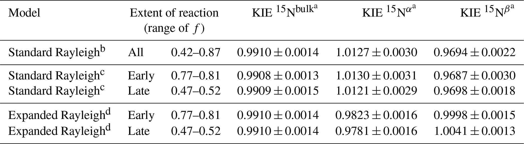
^a Average value ± standard deviation. ^b KIE values were calculated from ε_N-bulk, ε_N−α, or ε_N−β values obtained via linear regression of δ¹⁵N^bulk, δ¹⁵N^α, or δ¹⁵N^β against [$-f\ln f/(\mathrm{1}-f)$]. The standard Rayleigh model values presented here differ slightly from the previously published values (Yang et al., 2014) due to our exclusion of the earliest observation(s) from each replicate (i.e., observations with the highest values of f were excluded). ^c For the standard Rayleigh model applied to individual observations, ε_N-bulk, ε_N−α, or ε_N−β values were determined using Eq. (S24); the y intercept listed in that equation corresponds to the y intercept of δ¹⁵N^bulk, δ¹⁵N^α, or δ¹⁵N^β against [$-f\ln f/(\mathrm{1}-f)$] (determined by linear regression of the data from each replicate). KIE values for six (early) or seven (late) individual observations were pooled and averaged. ^d For the Expanded Rayleigh model applied to individual observations, bulk values (α_N-bulk, ε_N-bulk, and KIE ¹⁵N^bulk) were determined with the standard Rayleigh approach. ρ was calculated for each observation using Eq. (23) (ρ= ¹⁵N${}^{\mathit{\alpha }}{/}^{\mathrm{15}}$N^bulk), and τ was determined for every step of the reaction using Eq. (24) (τ=¹⁴N${}^{\mathit{\alpha }}{/}^{\mathrm{14}}$N^bulk). Then α_N−α and α_N−β were calculated for each individual observation with Eq. (21) or Eq. (22) and converted to KIE values using Eq. (10). KIE ¹⁵N^α and KIE ¹⁵N^β values for six (early) or seven (late) individual observations were pooled and averaged.

At present, there is a scarcity of studies reporting N₂O fractionation by purified enzymes for multiple values of f, limiting our ability to test the Expanded Rayleigh model with published experimentally derived datasets. We were, however, able to apply the Expanded Rayleigh model to previously published data on M. trichosporium cultures (Sutka et al., 2006), whose HAO-catalyzed oxidation of NH₂OH was the primary source of N₂O and displayed constant values of ε_N-bulk and SP. Thus, we were able to calculate observed values of KIE ¹⁵N^α and KIE ¹⁵N^β that serve as reasonable estimates of HAO-specific isotope effects (Table 5). Additionally, we have used the Expanded Rayleigh model to re-evaluate isotopic data our group has collected for purified fungal P450 NOR (Table 6) (Yang et al., 2014). The value of ε_N-bulk for P450 NOR appears to be constant, but SP increased by 14 ‰ as the fraction of NO reduced changed from 10 % to 50 % (Yang et al., 2014). Given the proposed P450 NOR reaction mechanism, the observed isotope effect for the first NO molecule is influenced by both an equilibrium isotope effect related to NO binding and an intrinsic KIE associated with catalysis (Yang et al., 2014). Conversely, the rate-determining steps for the second NO molecule are likely only associated with catalysis. Thus, the isotopic fractionation for the first nitrogen atom to be incorporated will be more sensitive to changes in NO concentration as the reaction progresses than the second N atom, leading to SP values that are not constant. Even in these circumstances, however, the Expanded Rayleigh model estimates for KIE ¹⁵N^α and KIE ¹⁵N^β are a significant improvement on the previously published standard Rayleigh estimates, which incorrectly predict a normal isotope effect at the α position. Overall, the Expanded Rayleigh model fits the available data on isotopic fractionation during N₂O biosynthesis reasonably well, although we recommend collecting isotopic data across a range of f values to confirm that SP (and therefore KIE ¹⁵N^α and KIE ¹⁵N^β) remains constant when using this model.

As outlined above (in the Assumptions section), the Expanded Rayleigh model is most accurate for reactions where the isotopic fractionation factors (ε_N-bulk, ε_N−α, and ε_N−β) and δ¹⁵N^s0 values are not too extreme. This stipulation, which also applies to the standard Rayleigh equation, is necessary in part because an approximation introduced by Mariotti and colleagues (Mariotti et al., 1981) decreases in accuracy the farther δ¹⁵N^s0 and δ¹⁵N^s are from 0 ‰. Additionally, extremely high positive values of δ¹⁵N^s0 or ε_N-bulk would result in large positive product δ values, corresponding to an increased abundance of ¹⁵N in the product. As both the nonlinear Rayleigh model and the underlying calculation of δ¹⁵N^β values depend on the assumption that the amount of ¹⁵N in N₂O is close to the natural abundance, the accuracy of the Expanded Rayleigh model would decrease in such circumstances. Thus, applying the Expanded Rayleigh model to experiments with spiked ¹⁵N is not advised. Simulations of δ values calculated without using Mariotti's approximation indicate that for absolute values of ε_N-bulk or δ¹⁵N^s0 less than or equal to 50 ‰, the level of error introduced by Mariotti's approximation is similar to the expected level of experimental error (i.e., absolute relative difference in KIE values of ∼ 0.001) (Tables S1–2).

The magnitude of ε_N−α and ε_N−β must also be considered when applying the Expanded Rayleigh model. In theory, if isotopic enrichment at N^α or N^β is very large, the assumption that essentially equal amounts of ¹⁴N are apportioned to each position (i.e., that τ≈0.5) would be violated, and Eq. (15) would no longer hold. However, violating this assumption would require unusually large heavy-atom kinetic isotope effects or a spiked sample. As outlined in Table S3, for a simulated reaction where ε_N-bulk is set at −20 ‰ (KIE ¹⁵N^bulk= 1.0204) and δ¹⁵N^s0 is 0 ‰, individual KIE values would have to be significantly lower than 0.96 or greater than 1.08 to introduce error greater than analytical error. These KIE ¹⁵N^α or KIE ¹⁵N^β values correspond to ρ values less than 0.47 or greater than 0.53. In practice, our group has found that for two different types of N₂O-producing enzymes, ρ is nowhere near these extremes. For example, for purified P450 NOR (Yang et al., 2014) and for HAO-catalyzed NH₂OH oxidation in an axenic culture (Sutka et al., 2006), ρ does not exceed 0.509 (Tables S15 and S17). Overall, we anticipate that the Expanded Rayleigh model will be applicable to a wide variety of N₂O biosynthesis reactions.

4.2 Other practical considerations

The Expanded Rayleigh model presented here does not require measurement of δ¹⁵N^s0. This is advantageous for N₂O synthesis reactions where NO is the substrate because directly measuring an accurate δ¹⁵N value for NO is quite challenging due to the reactivity of NO, the lack of isotopic standards for NO, and the fact that ¹⁴N¹⁶O has the same molecular weight as ¹⁵N¹⁵N. However, δ¹⁵N^s0 can be directly measured when NH₂OH is used as the substrate for N₂O production. Determining δ¹⁵N^s0 experimentally may be useful in validating application of the standard Rayleigh model, as the intercept of the standard Rayleigh model is expected to be equal to δ¹⁵N^s0. For example, we determined that the intercept of the standard Rayleigh plot for N₂O produced by NH₂OH oxidation by M. trichosporium is 0.5 ± 0.3 ‰, which is similar to the measured δ¹⁵N^s0 value of −2.3 ‰ (Sutka et al., 2006), confirming that the standard Rayleigh model is applicable for this dataset. Thus, when feasible, measuring δ¹⁵N^s0 would complement the expanded Rayleigh approach.

The nonlinear portion of the Expanded Rayleigh model (used to determine ρ) can be written in two forms, nonlinear model 1 (Eq. 29) and nonlinear model 2 (Eq. 30). Both models are based on the assumption that δ¹⁵N^bulk is equal to the average of δ¹⁵N^α and δ¹⁵N^β (Eq. 15). Therefore, both models are expected to produce very similar results as long as that assumption holds. Indeed, as we have demonstrated here, both models yield nearly identical values of ρ, KIE ¹⁵N^α, and KIE ¹⁵N^β for simulated datasets (Figs. 6 and S5–8; Tables S9–13), and we have obtained similar results for the available experimental data on N₂O production from NH₂OH (Table 5). Thus, either version of the Expanded Rayleigh model may be used. If there is any doubt about which version to use, we recommend selecting the model that has a lower RMSE value (and thus fits the data better).

5 Conclusions

In this paper, we presented the Expanded Rayleigh model, a novel adaptation of the Rayleigh distillation equation that describes the position-specific isotopic enrichment that occurs at N^α and N^β during N₂O synthesis. Using simulated datasets representing multiple different combinations of KIEs, we demonstrated that the Expanded Rayleigh model accurately recapitulates KIE ¹⁵N^α and KIE ¹⁵N^β for a wide variety of scenarios. Our simulations also demonstrate that this new model is robust even when applied to skewed data and/or data with a high level of error. Additionally, we have shown the Expanded Rayleigh model fits the experimentally measured isotopic data for N₂O production from NH₂OH quite well (Sutka et al., 2006) and provides significantly improved estimates for the position-specific KIEs for P450 NOR-catalyzed N₂O synthesis. Thus, the Expanded Rayleigh model provides a reliable method for quantifying isotopic fractionation at N^α and N^β, and it promises to be a valuable tool for experimentally probing the catalytic mechanisms of N₂O-synthesizing enzymes. Finally, we note that the Expanded Rayleigh model will also likely be appropriate for the analysis of other reactions where two atoms from the same substrate pool are incorporated into distinct, non-exchangeable positions in the product.