Hydrological cycle amplification imposes spatial patterns on the climate change response of ocean pH and carbonate chemistry

​​​​​​​Ocean CO₂ uptake and acidification in response to human activities are driven primarily by the rise in atmospheric CO₂ but are also modulated by climate change. Existing work suggests that this “climate effect” influences the uptake and storage of anthropogenic carbon and acidification via the global increase in ocean temperature, although some regional responses have been attributed to changes in circulation or biological activity. Here, we investigate spatial patterns in the climate effect on surface ocean acidification (and the closely related carbonate chemistry) in an Earth system model under a rapid CO₂-increase scenario and identify a different driving process. We show that the amplification of the hydrological cycle, a robustly simulated feature of climate change, is largely responsible for the spatial patterns in this climate effect at the sea surface. This “hydrological effect” can be understood as a subset of the total climate effect, which includes warming, hydrological cycle amplification, circulation, and biological changes. We demonstrate that it acts through two primary mechanisms: (i) directly diluting or concentrating dissolved ions by adding or removing freshwater and (ii) altering the sea surface temperature, which influences the solubility of dissolved inorganic carbon (DIC) and acidity of seawater. The hydrological effect opposes acidification in salinifying regions, most notably the subtropical Atlantic, and enhances acidification in freshening regions such as the western Pacific. Its single strongest effect is to dilute the negative ions that buffer the dissolution of CO₂, quantified as alkalinity. The local changes in alkalinity, DIC, and pH linked to the pattern of hydrological cycle amplification are as strong as the (largely uniform) changes due to warming, explaining the weak increase in pH and DIC seen in the climate effect in the subtropical Atlantic Ocean.

1 Introduction

The increasing atmospheric concentration of carbon dioxide (CO₂) causes a flux of CO₂ into the ocean, typically termed the “CO₂-concentration feedback” (e.g., Williams et al., 2019) (here, we will use the term “CO₂ effect”). This oceanic CO₂ uptake increases the total carbon content of the ocean (total dissolved inorganic carbon; DIC), decreases the availability of buffering ions (alkalinity or Alk), and consequently leads to ocean acidification (decrease in pH: $-{\log }_{\mathrm{10}}\left[{\mathrm{H}}^{+}\right]$). This study links the enhancement of the hydrological cycle with warming to regional changes in DIC, alkalinity, and acidification, thus linking a robust physical response of the climate system to a biological impact of climate change. Ocean acidification reduces the stability of solid calcium carbonate, weakening the protective shells of marine organisms, with negative impacts already visible, for example on tropical coral reefs (e.g., Caldeira and Wickett, 2003; Gattuso et al., 2014). Together with other stressors, including warming and ocean deoxygenation, acidification increases the vulnerability of certain marine organisms. For example, combined acidification and low oxygen levels narrow the range of temperatures at which organisms can function, and warming tends to increase baseline metabolic rates, further narrowing this thermal window (e.g., Pörtner, 2012; Doney et al., 2020; Kroeker et al., 2013).

Chemical changes in DIC, alkalinity, and pH are also modulated by climate change, via warming, circulation, freshwater flux, and biological changes. These effects can be isolated from the direct CO₂ effect as a separate “carbon–climate feedback” (here we will use the term “climate effect”, including all changes other than the atmospheric CO₂ increase, i.e., temperature, circulation, freshwater flux, and biological changes). This climate effect has been shown to decrease global CO₂ uptake and storage by approximately 10 % in projections of high-carbon-emissions scenarios (Arora et al., 2013; Friedlingstein and Prentice, 2010; Williams et al., 2019; McNeil and Matear, 2007; Schwinger et al., 2014). The best understood facet of the climate effect on seawater chemistry is warming, which drives a decrease in anthropogenic carbon uptake due to weakened solubility and ventilation (Katavouta and Williams, 2021). However, Katavouta and Williams (2021) also note that some regional patterns cannot be accounted for by these two processes, and indeed other studies have suggested that more complex shifts in circulation patterns and changes in biological activity contribute to regional climate effects on carbon storage in the interior (e.g., Lovenduski et al., 2008; Siedlecki et al., 2021; Pilcher et al., 2019). Although these studies demonstrate that regional variations in the climate effect are not exclusively related to warming, they are focused on anthropogenic carbon uptake and do not address the net effect of DIC and alkalinity changes on regional ocean acidification. McNeil and Matear (2007) describe the climate effect on ocean acidification and point out that warming has a direct effect in decreasing pH and an indirect effect in decreasing the solubility of CO₂, which limits acidification. They find that the net of these direct and indirect effects is small on a global average but did not address the larger regional responses, which are critical for anticipating ecosystem impacts. Here, we find that the amplification of the hydrological cycle with warming, a robust response of climate models to global warming that has recently been linked to patterns of ocean oxygen loss with climate change (Hogikyan et al., 2024), is in fact responsible for the bulk of the spatial pattern in surface ocean DIC and alkalinity and consequently acidification attributed to the climate effect.

The “hydrological cycle amplification” reinforces sea surface salinity (SSS) patterns, leading to a “salty-get-saltier, fresh-get-fresher” rule of thumb for changes in SSS, especially at low and mid-latitudes where the hydrological cycle is strongest (Durack and Wijffels, 2010). Specifically, hydrological cycle amplification refers to enhanced spatial patterns of net air–sea freshwater fluxes (precipitation–evaporation), which are largely responsible for the mean SSS patterns (Held and Soden, 2006; Manabe and Wetherald, 1975). Hydrological cycle amplification can induce regional patterns in surface seawater carbonate chemistry in two ways. First, freshwater fluxes can directly change the concentration of dissolved species, potentially increasing the concentrations of DIC and alkalinity in salty-get-saltier regions and decreasing their concentrations in fresh-get-fresher regions. pH increases with DIC and decreases with alkalinity so that freshwater fluxes drive a small net change in pH. Second, these changes in salinity modify the ocean circulation and lead to a net increase in ocean heat uptake globally, which weakens surface warming (as shown by Liu et al., 2021; Williams et al., 2007). This heat uptake is due to enhanced subduction in regions of sea surface strong salinity increase, primarily the North Atlantic. This relative cooling could drive an increase in DIC and pH, weakening the influence of warming in the total climate effect.

We estimate the regional DIC, alkalinity, and pH changes due to (a) the total climate effect and (b) the subset of the climate effect due only to hydrological cycle amplification – the “hydrological effect” – using a high-CO₂-increase scenario in a global Earth system model (NOAA-GFDL's ESM2M; Dunne et al., 2013). The experiments follow those used to isolate the hydrological effect on ocean oxygen loss in Hogikyan et al. (2024). We focus on the sea surface, where the response to hydrological cycle amplification is largest, and separate the surface into a fresh-get-fresher and a salty-get-saltier regime; the changes in these two regimes largely cancel in the global average but could modify local carbonate chemistry and its biological impacts. Then, we further attribute the climate effect and hydrological effect DIC, alkalinity, and pH changes to two primary mechanisms: (a) freshwater (dilution and concentration of DIC and alkalinity), and (b) thermal (temperature-driven) effects. We find that hydrological cycle amplification can account for much of the regional pattern in the total climate effect, since it is the sole driver of long-term trends in freshwater fluxes, while temperature changes are more spatially uniform. We show that these freshwater fluxes change the concentration of alkalinity slightly more than that of DIC due to the mean chemistry of the ocean, with the consequence that DIC and pH tend to increase along with alkalinity in salty-get-saltier regions and decrease in fresh-get-fresher regions.

2 Methods

2.1 Earth system model and experiments to isolate hydrological and climate effects

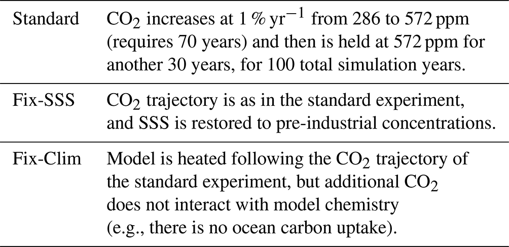
We use the Geophysical Fluid Dynamics Laboratory Earth System Model 2M (ESM2M), which is fully described in Dunne et al. (2012, 2013). The version of ESM2M used here (public release 5.0.2, available at: https://github.com/mom-ocean/MOM5/blob/master/doc/web/quickstart.md, last access: 21 October 2024) uses the atmosphere model AM2 with a horizontal resolution of approximately 50 km and the ocean model MOM5 with a horizontal resolution of approximately 100 km, as well as the land model LM3.0 and ocean biogeochemical model TOPAZ2. In order to isolate the signature of increasing atmospheric CO₂ and the associated amplification of the hydrological cycle, we force the model with a strong atmospheric CO₂ increase of 1 % yr⁻¹, beginning from the pre-industrial concentration of 286 ppm, until the CO₂ level doubles after 70 years. During years 71–100 the CO₂ level is held fixed at double the pre-industrial concentration (562 ppm) so that the entire experiment is 100 years long. We compare three different experiments with this 1 %-to-doubling CO₂ forcing. This is identical to the experimental setup used in Hogikyan et al. (2024), and further details can be found therein. The spatial patterns of salinity changes agree with long-term trends in observations and other climate models.

In the first experiment, the model freely responds to the prescribed atmospheric CO₂ (“standard”), and the strength of the hydrological cycle intensifies with warming, amplifying patterns of freshwater fluxes and SSS. In the second experiment, SSS is nudged towards its pre-industrial monthly climatology with a restoring flux of freshwater (“Fix-SSS”) as CO₂ increases along the same 1 %-to-doubling trajectory. There is no restoring under seasonal sea ice. The freshwater restoring flux dilutes (or concentrates) all chemical species, although SSS is used to determine its strength. The difference between the standard and Fix-SSS experiments provides an estimate of the impact of the hydrological cycle amplification on the ocean (including the direct freshwater flux and ocean circulation adjustment), and for a given variable X we define the change due to hydrological cycle amplification, the hydrological effect, in terms of the difference between these two simulations:

$$\mathrm{\Delta }{X}_{\mathrm{hydro}}=X_{\mathrm{standard}}-X_{\mathrm{Fix}\text{-}\mathrm{SSS}}.$$

To contextualize the hydrological effect as a part of the total carbon–climate feedback, or climate effect, we also run a fixed-climate experiment in which the same 1 %-to-doubling atmospheric CO₂ increase interacts with ocean biogeochemistry but not with radiation so that there is no global warming (no change in climate). In this experiment, the ocean experiences carbon uptake due to atmospheric CO₂ increase but no warming or hydrological cycle amplification. The climate effect can therefore be defined by

$$\mathrm{\Delta }{X}_{\mathrm{clim}}=X_{\mathrm{standard}}-X_{\mathrm{Fix}\text{-}\mathrm{Clim}}$$

(e.g., Williams et al., 2007, 2019; Katavouta and Williams, 2021). In this framework, we define X_standard, X_Fix-Clim, and X_Fix-SSS using the average over the last 30 years of each simulation (years 71–100) when atmospheric CO₂ is held steady at double the pre-industrial concentration and the system is beginning to equilibrate at this higher CO₂ level, to decrease the influence of internal variability or rapid adjustments to forcing. Results are presented for the Atlantic, Indian, and Pacific oceans, with a focus on the low latitudes and mid-latitudes, where the hydrological cycle is most active, i.e., where the amplification of evaporation–precipitation patterns is strongest. We ignore high latitudes, where the surface freshwater balance is instead dominated by ice–ocean interactions (north of 55° S and with a mask applied where seasonal sea ice is found in the pre-industrial control run; see mask in Fig. 1).

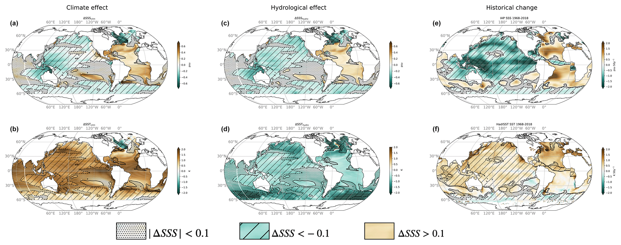
Figure 1 Sea surface salinity (SSS) and temperature (SST) changes associated with climate and hydrological effects. (a, b) SSS and SST change with climate effect (standard minus Fix-Clim experiments), which includes the hydrological effect and other changes, notably global warming; (c, d) SSS and SST change with hydrological effect (standard minus Fix-SSS experiments), which weakens surface warming and reinforces SSS patterns. Also shown for comparison is the recent historical linear trend pattern in (e) SSS and (f) SST, as quantified by the Institute for Atmospheric Physics reanalysis (Cheng et al., 2017) and the HadISST analysis product (Rayner et al., 2003). Stippling indicates regions where ΔSSS_hydro is small (| ΔSSS_hydro |< 0.1 psu); these regions are excluded from our analysis. Hatching indicates the fresh-get-fresher regime where ΔSSS_hydro< −0.1 psu. A lack of hatching indicates the salty-get-saltier regime where ΔSSS_hydro > +0.1 psu. See Table 1 for description of experiments.

ΔX_clim includes a contribution from ΔX_hydro as well as from other changes. For instance, the climate effect includes a strong increase in sea surface temperature (SST) so that ΔSST_clim is positive (i.e., SST_standard exceeds SST_Fix-Clim at the end of the simulation; Fig. 1c). However, the hydrological cycle amplification moderates surface warming by enhancing ocean heat uptake (Williams et al., 2007; Liu et al., 2021) so that ΔSST_hydro is negative (i.e., SST_standard is less than SST_Fix-SSS at the end of the simulation; Fig. 1d).

All model experiments, as well as the abbreviations we use to reference them, are summarized in Table 1.

Table 1 Simulation definitions.

2.2 Freshwater and thermal contributions to DIC and alkalinity changes

We quantify the influence of freshwater fluxes (dilution/concentration of DIC and alkalinity) and temperature changes on DIC and alkalinity in both the hydrological effect (the amplification of the hydrological cycle, represented by the standard – Fix-SSS experiments) and the climate effect (the total effect of climate change including warming, hydrological cycle amplification, etc., represented by the standard – Fix-Clim experiments).

DIC is affected by both freshwater fluxes and temperature changes so that we can decompose ΔDIC_hydro as follows:

$$\mathrm{\Delta }{\text{DIC}}_{\mathrm{hydro}}=\mathrm{\Delta }{\text{DIC}}_{\mathrm{FW},\mathrm{hydro}}+\mathrm{\Delta }{\text{DIC}}_{\mathrm{thermal},\mathrm{hydro}}+R_{\mathrm{DIC},\mathrm{hydro}},$$

where ΔDIC_FW, hydro and ΔDIC_{thermal, hydro} correspond to contributions from dilution or concentration by freshwater (FW) fluxes and changes due to a temperature change (thermal). The residual R includes all other processes that affect DIC and alkalinity (e.g., air–sea fluxes of CO₂, calcium carbonate precipitation–dissolution, production and remineralization of organic matter, and salinity) as well as co-variations between the thermal and freshwater effects and errors in our method of estimating these effects (which are elaborated on below).

In contrast, alkalinity does not vary with temperature. Its hydrological effect can be approximated as

$$\mathrm{\Delta }{\text{Alk}}_{\mathrm{hydro}}=\mathrm{\Delta }{\text{Alk}}_{\mathrm{FW},\mathrm{hydro}}+R_{\mathrm{Alk},\mathrm{hydro}}.$$

We can attribute the total climate effect in DIC and alkalinity to freshwater and thermal effects, following the same framework:

$$\begin{array}{c}\mathrm{\Delta }{\text{DIC}}_{\mathrm{clim}}=\mathrm{\Delta }{\text{DIC}}_{\mathrm{FW},\mathrm{clim}}+\mathrm{\Delta }{\text{DIC}}_{\mathrm{thermal},\mathrm{clim}}+R_{\mathrm{DIC},\mathrm{clim}}\\ \mathrm{\Delta }{\text{Alk}}_{\mathrm{clim}}=\mathrm{\Delta }{\text{Alk}}_{\mathrm{FW},\mathrm{clim}}+R_{\mathrm{Alk},\mathrm{clim}}.\end{array}$$

The various residuals R are quantified in Figs. A1 and A2. We are largely successful in reconstructing the hydrological effect, and R is generally small relative to ΔDIC_hydro and ΔAlk_hydro (error < 5 µmol kg⁻¹ at a point relative to broad regional changes of 15–40 µmol kg⁻¹; Figs. 2, A1. Note AX indicates Appendix Fig. X). The error is somewhat more significant in reconstructing the climate effect (ΔDIC_clim and ΔAlk_clim; Fig. A2), especially for DIC (error <8 µmol kg⁻¹). This is most likely due to the fact that the climate effect leads to anomalous air–sea CO₂ fluxes (primarily due to warming but possibly also influenced by circulation changes), which change DIC and can indirectly lead to changes in alkalinity.

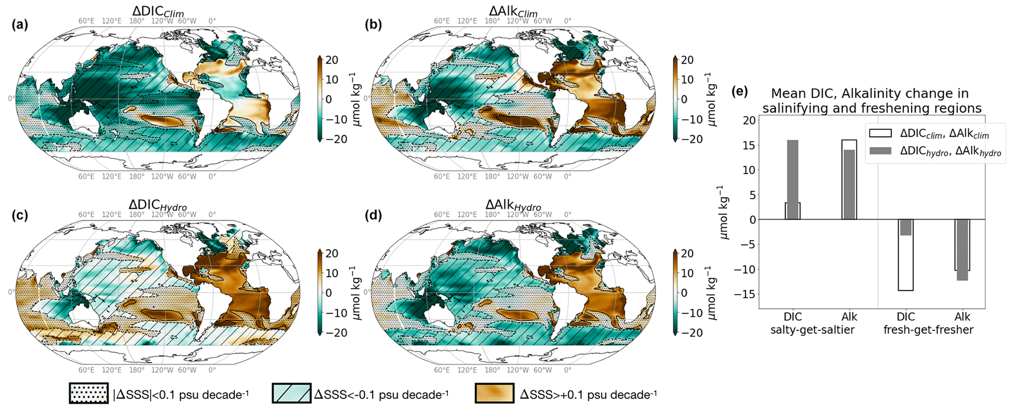
Figure 2 DIC and alkalinity response to climate and hydrological effects. Change in surface (a) DIC and (b) alkalinity due to the climate effect (standard minus Fix-Clim experiments); change in surface (c) DIC and (d) alkalinity due to the hydrological effect (standard minus Fix-SSS experiments). (e) Mean change in DIC (black) and alkalinity (grey) in salinifying (ΔSSS_hydro > 0.1 psu) and freshening (ΔSSS_hydro < −0.1 psu) regions shown in Fig. 1. For panels (a)–(d), stippled areas experience nearly zero change in salinity (|ΔSSS_hydro| < 0.1 psu) and are ignored in our analysis, while fresh-get-fresher regions are hatched (ΔSSS_hydro < −0.1 psu), and salty-get-saltier regions have no hatching (ΔSSS_hydro > +0.1 psu). See Table 2 for definitions.

We quantify the effect of freshwater fluxes on alkalinity and DIC (ΔAlk_FW, hydro, ΔDIC_FW, hydro) with a simple conservation argument which neglects the effects of mixing and advection, a fair approximation within the mixed layer. In this case, DIC, alkalinity, and salt are diluted/concentrated by air–sea freshwater fluxes by the same fraction $f_{\mathrm{FW},\mathrm{hydro}}=\mathrm{\Delta }{S}_{\mathrm{hydro}}/S_{\mathrm{Fix}\text{-}\mathrm{SSS}}$ referenced to salinity (S). For example, if a freshwater flux into the surface in the standard warming experiment diluted SSS by f_FW, hydro = 5 % compared to the Fix-SSS experiment (i.e., SSS_standard = 0.95 SSS_Fix-SSS), then surface DIC and alkalinity would also be diluted by f_FW, hydro = 5 % from the reference Fix-SSS concentrations (DIC_standard = 0.95 DIC_Fix-SSS; Alk_standard = 0.95 Alk_Fix-SSS). We can therefore approximate ΔDIC_FW, hydro and ΔAlk_FW, hydro as

$$\begin{array}{}\text{(1)}& \begin{array}{l}\mathrm{\Delta }{\text{Alk}}_{\mathrm{FW},\mathrm{hydro}}=f_{\mathrm{FW},\mathrm{hydro}}{\text{Alk}}_{\mathrm{Fix}\text{-}\mathrm{SSS}},\\ \mathrm{\Delta }{\text{DIC}}_{\mathrm{FW},\mathrm{hydro}}=f_{\mathrm{FW},\mathrm{hydro}}{\text{DIC}}_{\mathrm{Fix}\text{-}\mathrm{SSS}}.\end{array}\end{array}$$

The effects of mixing and transport on salinity are included in f_FW, because it is derived from changes in salinity. However, since mixing and transport act on different spatial gradients for each variable, f_FW cannot be expected to be the same for salinity, DIC, Alk, etc., except in the mixed layer where gradients are relatively weak for all constituents. As a consequence, we restrict our analysis to the mixed layer, where this error is very small relative to the changes driven by temperature and freshwater effects (as demonstrated in Figs. 3, A1, and A2).

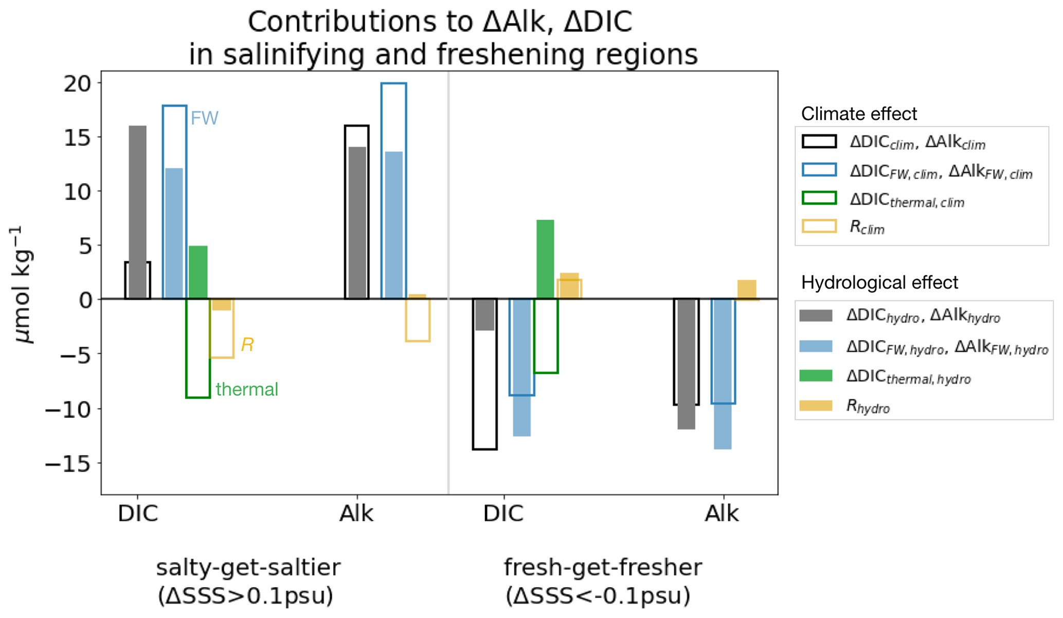
Figure 3 Thermal and freshwater components of DIC and alkalinity changes in fresh-get-fresher and salty-get-saltier regions. Change in surface DIC and alkalinity concentrations in response to the climate effect (empty bars) and the hydrological effect (filled bars) in salinifying and freshening regions (as in Figs. 4c and 2e). Black and grey bars represent total Δ_clim and Δ_hydro and are identical to those in Fig. 2e. Blue bars represent change in DIC or alkalinity due to freshwater fluxes. Green bars represent change in DIC due to SST change. See Table 2 for definitions of components.

We estimate DIC changes due to thermal changes following Sarmiento (2006), using a constant thermal sensitivity $\frac{\partial \text{DIC}}{\partial T}$ of −7 $\mathrm{\mu }\mathrm{mol}{\mathrm{kg}}^{-\mathrm{1}}{\mathrm{K}}^{-\mathrm{1}}$:

$$\mathrm{\Delta }{\mathrm{DIC}}_{\mathrm{thermal},\mathrm{hydro}}={\displaystyle \frac{\partial \text{DIC}}{\partial T}}\mathrm{\Delta }{T}_{\mathrm{hydro}}=-\mathrm{7}\mathrm{\Delta }{T}_{\mathrm{hydro}}.$$

This approximation introduces some error since $\frac{\partial \text{DIC}}{\partial T}$ is not constant, but we find that our results do not change if we allow the sensitivity to vary at each model grid point and month. Our conclusions are not sensitive to the choice of constant within a range of 7 ± 2 $\mathrm{\mu }\mathrm{mol}{\mathrm{kg}}^{-\mathrm{1}}{\mathrm{K}}^{-\mathrm{1}}$.

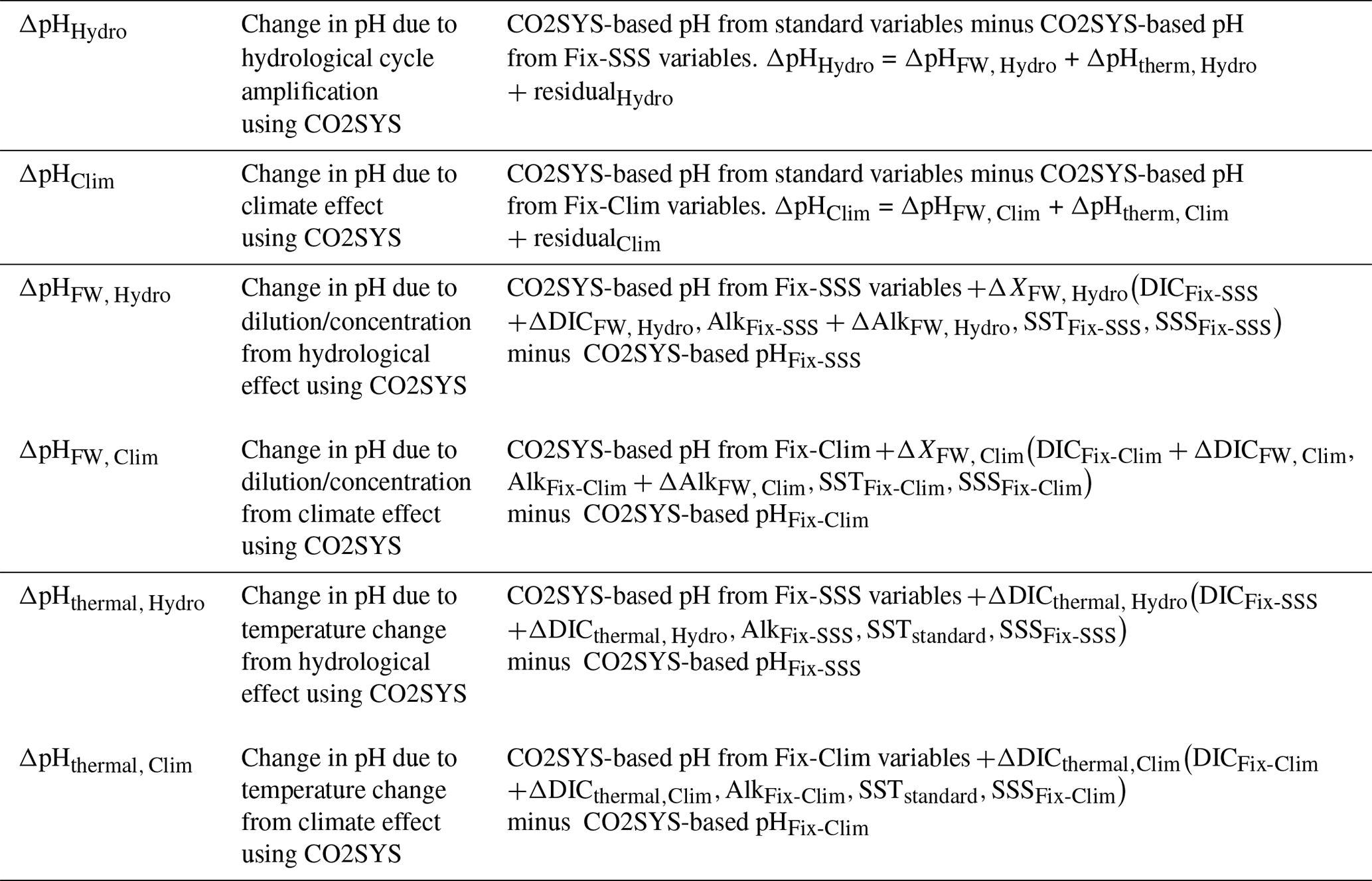
The decomposition of DIC and Alk changes laid out above is also summarized in Table 2.

Table 2 ΔDIC and ΔAlk component definitions. X stands for DIC and Alk.

2.3 Attribution of surface pH changes to hydrological and climate effects

Equilibrium pH can be understood as a nonlinear function of DIC, alkalinity, temperature (T), and salinity (S) so that a difference in pH between two model experiments or ocean chemical states can be interpreted in terms of the corresponding changes in DIC, alkalinity, temperature, and salinity between these two states (e.g., as in García-Ibáñez et al., 2016). An increase in DIC due to CO₂ dissolution produces H⁺ ions and decreases pH, whereas an increase in alkalinity represents a greater seawater buffering capacity and yields a higher pH. Temperature has a direct negative relationship with pH (warming ionizes water, thus decreasing pH) and an indirect positive relationship with pH (the solubility of DIC decreases with temperature and leads to an increase in pH). Salinity has a small effect on pH and will not be discussed in this study.

We define the hydrological effect and climate effect on pH as

$$\begin{array}{}\text{(2)}& {\displaystyle }\begin{array}{rl}& \mathrm{\Delta }{\text{pH}}_{\mathrm{hydro}}=\text{pH}\left({\text{DIC}}_{\mathrm{Std}},{\text{Alk}}_{\mathrm{Std}},T_{\mathrm{Std}},S_{\mathrm{Std}}\right)\\ & -\text{pH}\left({\text{DIC}}_{\mathrm{Fix}\text{-}\mathrm{SSS}},{\text{Alk}}_{\mathrm{Fix}\text{-}\mathrm{SSS}},T_{\mathrm{Fix}\text{-}\mathrm{SSS}},S_{\mathrm{Fix}\text{-}\mathrm{SSS}}\right),\end{array}\text{(3)}& {\displaystyle }\begin{array}{rl}& \mathrm{\Delta }{\text{pH}}_{\mathrm{Clim}}=\text{pH}\left({\text{DIC}}_{\mathrm{Std}},{\text{Alk}}_{\mathrm{Std}},T_{\mathrm{Std}},S_{\mathrm{Std}}\right)\\ & -\text{pH}\left({\text{DIC}}_{\mathrm{Fix}\text{-}\mathrm{Clim}},{\text{Alk}}_{\mathrm{Fix}\text{-}\mathrm{Clim}},T_{\mathrm{Fix}\text{-}\mathrm{Clim}},S_{\mathrm{Fix}\text{-}\mathrm{Clim}}\right),\end{array}\end{array}$$

where the standard, Fix-SSS, and Fix-Clim pH are all estimated using the marine carbonate chemistry solver PyCO2SYS (Humphreys et al., 2022) to remove any biases between CO2SYS and the Earth system model. pH is a highly nonlinear function of other state variables and is solved for iteratively. We therefore make use of this established solver rather than making our own estimate, as we do for DIC and Alk. These ΔpH_Clim and ΔpH_Hydro estimates from CO2SYS are not identical to pH_Std−pH_Fix-Clim and pH_Std−pH_Fix-Hydro from the model experiments because CO2SYS assumes chemical equilibrium. (As a point of interest, ESM2M is constrained by the conservation of heat and mass in the coupled model, but a given location is not necessarily in chemical equilibrium.) We use this method because it allows us to break down ΔpH_hydro and ΔpH_Clim into freshwater (chemical dilution) and thermal (temperature-driven) components (as well as a residual due to errors in method and other drivers). The changes in pH are attributed to freshwater and thermal effects, similarly to DIC and alkalinity:

$$\mathrm{\Delta }{\text{pH}}_{\mathrm{hydro}}=\mathrm{\Delta }{\text{pH}}_{\mathrm{FW},\mathrm{hydro}}+\mathrm{\Delta }{\text{pH}}_{\mathrm{thermal},\mathrm{hydro}}+R.$$

Freshwater fluxes affect pH primarily through their effect on DIC and alkalinity; we use the DIC and alkalinity changes due to freshwater fluxes (as estimated in Sect. 2.2) to evaluate the freshwater flux effect on pH ΔpH_FW. The principle here is to take our estimates of the change in DIC and alkalinity due to freshwater fluxes and see what pH change is predicted to result (isolating the freshwater effect and ignoring other changes, e.g., temperature). More specifically, ΔpH_FW, hydro is defined as the difference between the theoretical pH with diluted/concentrated DIC and Alk (in bold) and the reference pH_Fix-SSS, which excludes the influence of hydrological cycle amplification:

$$\begin{array}{rl}& \mathrm{\Delta }{\text{pH}}_{\mathrm{FW},\mathrm{hydro}}=\text{pH}(\left({\mathbf{f}}_{\mathbf{FW},\mathbf{hydro}}+\mathbf{\text{1}}\right){\mathbf{\text{DIC}}}_{\mathbf{Fix}\text{-}\mathbf{SSS}},\\ & \left({\mathbf{f}}_{\mathbf{FW},\mathbf{hydro}}+\mathbf{\text{1}}\right){\mathbf{Alk}}_{\mathbf{Fix}\text{-}\mathbf{SSS}},{\text{SST}}_{\mathrm{Fix}\text{-}\mathrm{SSS}},{\mathrm{SSS}}_{\mathrm{Fix}\text{-}\mathrm{SSS}})\\ & -{\text{pH}}_{\mathrm{Fix}\text{-}\mathrm{SSS}}.\end{array}$$

We next want to ask what pH change should result from the temperature changes. However, we know that thermal changes in DIC (which we estimate above) co-occur with actual temperature changes, which also have a direct influence on pH. We define the thermally driven change in pH (ΔpH_thermal) to include these direct and indirect thermal effects (SST and DIC changes, respectively, emphasized in bold):

$$\begin{array}{rl}& \mathrm{\Delta }{\text{pH}}_{\mathrm{thermal},\mathrm{hydro}}=\text{pH}({\mathbf{DIC}}_{\mathbf{Fix}\text{-}\mathbf{SSS}}+\mathbf{\Delta }{\mathbf{DIC}}_{\mathrm{thermal},\mathrm{hydro}},\\ & {\mathrm{Alk}}_{\mathrm{Fix}\text{-}\mathrm{SSS}},{\mathbf{SST}}_{\mathbf{standard}},{\text{SSS}}_{\mathrm{Fix}\text{-}\mathrm{SSS}})\\ & -{\mathrm{pH}}_{\mathrm{Fix}\text{-}\mathrm{SSS}}.\end{array}$$

The decomposition of pH changes laid out above is also summarized in Table 3.

Table 3 ΔpH component definitions.

3 Results

3.1 Climate-driven DIC and alkalinity changes explained by hydrological effect

The climate model used here, ESM2M, responds to a CO₂ increase with surface warming and enhancement of mean salinity patterns. This results in a salinity increase in salty subtropical regions (enhanced in the Atlantic, relative to the Pacific) and a decrease in fresh regions, most notably high latitudes and the western tropical Pacific Ocean (Fig. 1a, b). These changes represent the climate effect in SST and SSS and are consistent with many prior studies (most notably Manabe and Wetherald, 1975; Held and Soden, 2006). Similar changes in both SST and SSS are seen in historical trends (Fig. 1e, f; see Durack and Wijffels, 2010). While this climate effect has been studied and hydrological cycle amplification is known to be a robust feature, the effect of hydrological cycle amplification (hydrological effect) has only been isolated more recently in Williams et al. (2007), Liu et al. (2021), and Hogikyan et al. (2024). As has been shown in these prior studies, the hydrological effect accounts almost exactly for the SSS changes in the climate effect. It also leads to surface cooling (due to enhanced global ocean heat uptake) (Fig. 1c, d). Please see Table 1 and Sect. 2 for an overview of the experiments we use to isolate the climate effect and hydrological effect.

We next assess the climate and hydrological effects on surface carbonate chemistry. For simplicity and clarity, we average over “saltier” and “fresher” ocean surface areas: specifically, where salinification is in excess of 0.1 psu (the (sub)tropical Atlantic and southeast Pacific oceans) and where freshening is stronger than −0.1 psu (the high-latitude Atlantic and remainder of the Indian and Pacific oceans; Figs. 2, 1). Although the DIC change has a similar spatial pattern as alkalinity, dictated by the sign of freshwater fluxes, we will show that its magnitude is modulated by a thermal component (warming in the climate effect and cooling in the hydrological effect). Where SSS increases, DIC is less sensitive than Alk to the climate effect (ΔDIC_clim = +2 µmol kg⁻¹ and ΔAlk_clim = +16 µmol kg⁻¹; see Table 2 for definitions), but they have the same sensitivity to the hydrological effect (ΔDIC_hydro = +16 µmol kg⁻¹ and ΔAlk_hydro = +14 µmol kg⁻¹). Where SSS decreases, the two have a similar response to the climate effect (ΔDIC_clim = −13 µmol kg⁻¹, while ΔAlk_clim = −10 µmol kg⁻¹; black empty bars in Fig. 2), but DIC is less sensitive than Alk to the hydrological effect (ΔDIC_hydro = −5 µmol kg⁻¹ and ΔAlk_hydro = −12 µmol kg⁻¹; grey bars in Figs. 2e and 3). We can understand what controls these changes in DIC and alkalinity by attributing them to freshwater (dilution/concentration), thermal, and residual (e.g., approximations in f_FW, as well as biological and circulation) effects using simple sensitivity estimates described in Sect. 2.

The effect of freshwater fluxes is very similar in both the hydrological effect and the climate effect, consistent with the understanding that hydrological cycle amplification accounts for the bulk of salinity changes in the total climate effect (Durack et al., 2012) (Fig. 1a, c; i.e., $f_{\mathrm{FW},\mathrm{hydro}}\approx f_{\mathrm{FW},\mathrm{clim}}$). However, the higher mean concentration of alkalinity makes alkalinity more sensitive to freshwater addition and removal than DIC (in both the total climate effect and hydrological effect; blue bars in Fig. 3, maps in Fig. A3). For example, when we evaluate (ΔX_FW, hydro = X_Fix-SSS f_FW, hydro), ΔAlk_FW, hydro is slightly greater than ΔDIC_FW, hydro due to the greater reference Alk_Fix-SSS (Fig. 3, blue bars). The freshwater effect in salty-get-saltier waters increases DIC and alkalinity by 17 and 19 µmol kg⁻¹ in the climate effect; the increase is slightly less in the hydrological effect, 12 and 14 µmol kg⁻¹. Dilution from freshening decreases DIC and alkalinity by −9 and −10 µmol kg⁻¹ in the climate effect. The freshwater effect on both DIC and Alk is slightly larger in the hydrological effect alone, −13 and −14 µmol kg⁻¹. These discrepancies between the hydrological and climate effects are primarily due to the discrepancy between dilution/concentration fractions f_FW, hydro and f_FW, clim, which arise from the difference in ocean circulation and salinity fields between the Fix-SSS and Fix-Clim experiments.

Changes in surface temperature substantially modify the DIC response to both the total climate effect and the hydrological effect since the solubility of DIC decreases with increasing temperature. Alkalinity, however, is not sensitive to temperature, and as a result its changes are well accounted for by the freshwater effect alone (yellow residual bars for Alk are much smaller than freshwater and total Alk changes; Fig. 3). Surface warming in the climate effect decreases DIC concentrations everywhere (by −9 µmol kg⁻¹ in salinifying and −7 µmol kg⁻¹ in freshening regions), while surface cooling in the hydrological effect increases DIC concentrations everywhere (by +5 µmol kg⁻¹ in salinifying and +7 µmol kg⁻¹ in freshening regions; Fig. 3 green bars). Overall, the SST and corresponding DIC changes are similar across salinifying and freshening regions (Figs. 1c, d and A3b, e), although circulation changes lead to some spatial patterns in the temperature response. For example, the weaker ΔDIC_{thermal, clim} in freshening, relative to salinifying, regions (−6 vs. −8 µmol kg⁻¹; Fig. 3) is a consequence of the SST decrease (and positive ΔDIC_thermal,clim) in the Labrador Sea associated with a weakening of the overturning circulation, a common transient response of climate models to global warming and North Atlantic freshening (Fig. 1) (Menary and Wood, 2018; Manabe and Stouffer, 1995). Similarly, the greater ΔDIC_{thermal,hydro} in freshening regions (+7 vs. +5 µmol kg⁻¹; Fig. 3) is a consequence of slightly stronger cooling at high latitudes, where deep isopycnal mixing enhances the surface temperature response, while the cooling in the salty (sub)tropics is weaker. Despite these small differences, the ΔDIC_{thermal,hydro} and ΔDIC_thermal,clim are uniform in sign and quite similar in magnitude in both regimes, leading to a contrast between the net climate and hydrological effects where ΔDIC_clim < ΔAlk_clim, while ΔDIC_hydro > ΔAlk_hydro (black empty and filled bars in Fig. 3). In summary, the sign and spatial pattern of DIC and alkalinity changes in both the climate effect and hydrological effect are determined by freshwater fluxes associated with hydrological cycle amplification, and the magnitude of DIC changes is further modulated by changes in SST.

This simple decomposition into freshwater and thermal effects leaves some of the simulated changes in DIC and alkalinity unexplained (with the residual error represented by the yellow bars in Fig. 3). Major processes that are not included in these freshwater and thermal effects include air–sea CO₂ fluxes and other adjustments of the carbonate system, spatial shifts in the atmospheric and oceanic circulations, and biological activity. Errors in our method are also included in the residual. Despite these omissions, the decomposition skillfully reconstructs the hydrological effect in both DIC and alkalinity (R_hydro < 2 µmol kg⁻¹ for both; see also Fig. A4), while residuals for the climate effect are slightly larger (R_clim ≈ 4–5 µmol kg⁻¹ for Alk and DIC; see also Fig. A4). Biases in alkalinity reconstruction are < 10 % of the total hydrological effect, suggesting that this simple estimate of dilution is a fairly effective estimate of the influence of hydrological cycle amplification on alkalinity. The residuals in DIC are broadly consistent with the influence of air–sea CO₂ fluxes. For instance, the decomposition of the hydrological effect for DIC is biased slightly high in salty-get-saltier regions, consistent with unaccounted-for CO₂ outgassing (a secondary effect of the DIC increase and thus pCO₂ increase), and the inverse is true in fresh-get-fresher regions (Fig. A5). Similarly, the negative bias (missing carbon) in the climate effect reconstruction in salinifying regions is consistent with anomalous CO₂ uptake linked to the decrease in DIC (Fig. A5). We were not able to develop a simple attribution of surface DIC changes to air–sea fluxes (as we can with freshwater fluxes and temperature changes) because the DIC change due to a given surface flux is sensitive to multiple factors, including the effects of mixing and advection, as well as the temperature, surface wind speed, and sea state.

3.2 Acidification weakened in salty-get-saltier regions and exacerbated in fresh-get-fresher regions

The climate effect tends to decrease surface pH, thereby re-enforcing the acidification associated with the rise in atmospheric CO₂ (ΔpH_clim < 0; Fig. 4a; see Sect. 2 and Table 3 for definitions of all ΔpH terms). We find, however, that on average, the climate effect enhances acidification more in fresh-get-fresher regions than in salty-get-saltier regions (−0.005 vs. −0.001; black empty bars in Fig. 4c). The hydrological effect (dilution/concentration of DIC and Alk, direct and indirect effect of SST decrease) contributes strongly to the changes in pH simulated in response to climate change and largely explains the contrast in magnitude between freshening and salinifying regions (Fig. 4). In particular, the hydrological effect contributes to the acidification in fresh-get-fresher regions such as subpolar oceans but opposes acidification in salty-get-saltier regions such as the subtropical Atlantic (−0.001 vs. +0.002 on average over freshening and salinifying regions; grey bars in Fig. 4c). Note that the climate-driven increase in pH simulated in the equatorial Pacific upwelling region cannot be accounted for by the hydrological effect (Fig. 4a–b) but is instead associated with the weakened upwelling of cold and high-DIC waters simulated in this region (Figs. 1b and 2a).

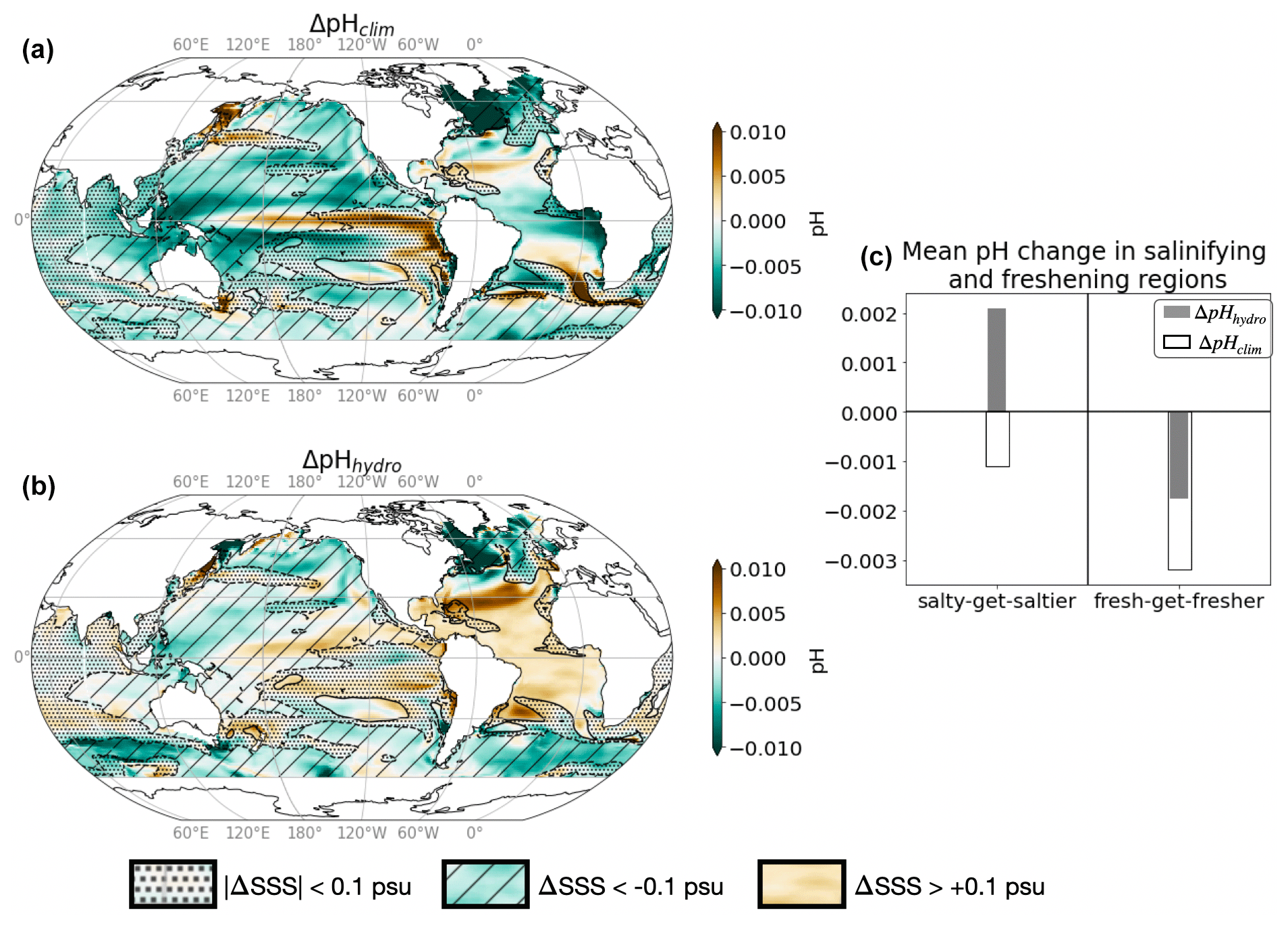
Figure 4 pH response to climate and hydrological effects. (a) Change in surface pH due to the climate effect (standard minus Fix-Clim experiments) and (b) hydrological effect (standard minus Fix-SSS experiments). Hatching indicates freshening ΔSSS_hydro < −0.1, while no hatching indicates salinity increase ΔSSS_hydro > 0.1. Black contours indicate ΔSSS_hydro = ±0.1 psu, and stippling indicates regions with small salinity changes, which are not considered in our analysis (|ΔSSS_hydro| < 0.1 psu). (c) Mean change in salinifying (left, ΔSSS_hydro > 0.1 psu) and freshening (right, ΔSSS_hydro < −0.1 psu) regions outlined in maps, with empty bars representing the climate effect and solid bars representing the hydrological effect. See Table 3 for definitions.

We next interpret these pH changes due to the climate and hydrological effects in terms of a thermal effect (which includes the opposing effects of DIC and SST on pH) and a freshwater flux effect (which includes the opposing effects of DIC and alkalinity on pH), using the thermal and freshwater components of DIC and alkalinity changes presented in Sect. 3 (Fig. 5).

Figure 5 Thermal and freshwater components of pH changes in fresh-get-fresher and salty-get-saltier regions. Change in surface pH in the climate effect (empty bars) and the hydrological effect (filled bars), in salty-get-saltier and fresh-get-fresher regions (as shown in Fig. 1). Black and grey bars represent total simulated pH change and are identical to those in Fig. 4c. Blue bars represent contribution of freshwater effect (via dilution of DIC and alkalinity). Green bars represent contribution of thermal effect (via SST change and DIC change due to SST). Yellow bars represent the residual (the difference between the sum of green + blue and the actual change represented by black and grey bars). See Table 3 for definitions of components.

The weakened acidification tied to the hydrological cycle in salinifying waters (i.e., an increase in pH tied to the hydrological effect) is attributed almost equally to the freshwater and thermal effects (filled bars in Fig. 5). pH has a similar sensitivity to both alkalinity and DIC in the modern surface ocean, and ΔAlk_FW always exceeds ΔDIC_FW (since the FW contribution scales with the mean value, and the mean alkalinity concentration is higher than the mean DIC concentration; see Sect. 2). As as result, the increasing ΔAlk_FW drives a positive ΔpH_FW in salty-get-saltier waters (Fig. 6c). At the same time, hydrological cycle amplification drives weak surface cooling (Liu et al., 2021), which further increases pH (McNeil and Matear, 2007). At lower latitudes where salty-get-saltier waters are found, the direct effect of cooling (cooling increases pH) overcomes the indirect effect (cooling increases DIC and reduces pH). Together, the increased alkalinity and decreased temperature increase pH, weakening the net acidification in the total climate effect. Similarly, the enhanced acidification in freshening waters is also attributed almost equally to the freshwater and thermal effects (filled bars in Fig. 5). The decrease in alkalinity due to freshwater input reinforces acidification. In this case, the indirect effect of cooling on pH exceeds the direct effect leading additional to acidification, in particular in cold, DIC-rich high-latitude waters, where the fresh-get-fresher signal is the strongest (Fig. 6d).

Figure 6 Contributions of temperature and freshwater flux changes to climate and hydrological effect. Upper row shows the contributions of (a) freshwater fluxes and (b) surface temperature change (warming) to the climate effect. Lower row shows the contributions of (c) freshwater fluxes and (d) surface temperature change (less warming) to the climate effect. Black contours indicate ΔSSS_hydro = ±0.1 psu, hatching indicates ΔSSS_hydro < −0.1, and no hatching indicates ΔSSS_hydro > 0.1. See Table 3 for definitions.

This decomposition into freshwater and thermal effects is insightful but simplistic. The combined freshwater and thermal effects correctly predict the sign of pH changes but better reconstruct the magnitude of the hydrological effect than of the climate effect (yellow residuals greater for climate effect in Fig. 5). The sum of these two components underestimates the magnitude of the total simulated pH decrease in the climate effect (predicting a weak decrease relative to the simulated ΔpH_clim of −0.001 and −0.003 in salinifying and freshening regions). The weakened air–sea CO₂ flux cannot explain the enhanced acidification, suggesting that this inaccuracy is related to error in our reconstructions of ΔAlk_FW, clim, ΔDIC_FW, clim, and ΔDIC_{thermal, clim}, which are discussed above, as well as the covariation between drivers of pH changes, which reflects the nonlinearity of the carbonate chemistry system.

Despite these limitations, the hydrological effect appears to contribute strongly to the spatial pattern of pH changes. The discrepancy in pH changes between the salty-get-saltier and fresh-get-fresher regions due to hydrological cycle amplification (nearly 0.004) is in fact larger than the discrepancy in the total climate effect (0.002). The hydrological effect introduces this strong pattern by (i) cooling of the surface and (ii) freshwater dilution in freshening regions and concentration in salinifying regions.

4 Discussion and conclusions

Our results suggest that the changes in alkalinity, DIC, and pH linked to hydrological cycle amplification contribute as strongly to the spatial pattern of the climate effect as warming alone, although these effects largely offset one another in the global mean. In fact, since alkalinity is not strongly influenced by temperature, nearly the entire climate effect in surface alkalinity is accounted for by the hydrological effect, i.e., dilution or concentration by anomalous freshwater fluxes (precipitation–evaporation). The climate effect includes a surprising DIC and pH increase (opposite the decreases expected from surface warming) in the subtropical Atlantic Ocean, as well as an exceptionally strong DIC decrease at higher latitudes. Both of these features can be largely accounted for by the hydrological effect. Although the freshwater loss from the (salty-get-saltier) subtropical Atlantic Ocean leads to an increase in both alkalinity and DIC, the increase in alkalinity is greater (and the DIC increase is weakened by the global cooling effect of hydrological cycle amplification), leading to a local increase in pH. The critical role of alkalinity in determining the response of marine carbonate chemistry to climate change here is consistent with prior studies (e.g., Chikamoto et al., 2023; Planchat et al., 2024). At high latitudes, the decrease in DIC associated with warming in the total climate effect is amplified by dilution (fresh-get-fresher) and tends to support stronger acidification. The nonlinear response of pH and other biologically important parameters (such as aragonite and/or calcite saturation states; e.g., Pinsonneault et al., 2012) are left to other studies to study in more detail.

Although this is the first study to isolate the hydrological effect on seawater carbonate chemistry, the amplification of the hydrological cycle itself and its impact on ocean heat uptake and SST have been shown to be consistent across ocean–atmosphere models, despite differences in core ocean and atmosphere components (Williams et al., 2007; Liu et al., 2021; Held and Soden, 2006). Because of these prior results, we expect the sign and magnitude of these results to remain similar across other models. This study attempts to explain the mechanisms driving patterns in the total climate effect for DIC, alkalinity, and pH and is intended to complement two recent studies on the influence of the hydrological effect on ocean heat uptake and ocean oxygen distribution (Liu et al., 2021; Hogikyan et al., 2024). We find regional changes due to the hydrological effect alone are on the same order of magnitude as the total climate effect and can explain the spatial patterning in the climate effect (±0.01 pH, ±20 µmol kg⁻¹ DIC, and ±20 µmol kg⁻¹ Alk), but both are of course smaller than the direct effect of CO₂ (in these simulations, approximately −0.2 pH, 120 µmol kg⁻¹ DIC, and 20 µmol kg⁻¹ Alk) (Williams et al., 2019). However, it is encouraging that we are able to clearly quantify this effect of freshwater fluxes even under relatively strong atmospheric CO₂ forcing, despite the strong nonlinearity of ocean carbonate chemistry.

The surface patterns in DIC and alkalinity presented here affect the distribution of carbon storage within the ocean. For example, the hydrological cycle leads to a slight increase in carbon storage in mode and intermediate waters at the expense of deeper water masses, while the total climate effect tends to decrease carbon uptake and storage everywhere. However, these changes (due to the total climate effect or the hydrological effect alone) are small in the ocean interior (generally $<\left|\mathrm{5}\right|$ µmol kg⁻¹).

Finally, it is worthwhile to note that our “freshwater” component is similar to the traditional salinity normalization, in that both make use of the fact that freshwater fluxes should change DIC and alkalinity approximately in proportion to salinity. However, we reference a spatially resolved pre-industrial control salinity to describe the effect of climate change rather than referencing the central estimates of 1900 µmol kg⁻¹ DIC, 2310 µmol kg⁻¹ Alk, and 35 psu used in the standard normalization (Broecker and Peng, 1992). Our method makes fewer assumptions and is slightly more precise but requires more data. Our study also demonstrates that this “freshwater effect” (which the salinity normalization is intended to remove) can have substantial consequences for carbonate chemistry, with implications for CO₂ fluxes, pH, etc. This result raises the question of how useful salinity-normalized values are. If one only examined the salinity-normalized CO₂, for example, one might struggle to explain changes in other carbonate system parameters, especially in a scenario with strong freshwater fluxes.

Appendix A

Figure A1 Ability of freshwater SST decomposition to reconstruct the spatial pattern of changes in surface DIC and alkalinity with the hydrological effect. Success of the freshwater effect (ΔAlk_FW, hydro) in predicting ΔAlk_hydro (a, b) and success of “freshwater + SST effects” ($\mathrm{\Delta }{\text{DIC}}_{\mathrm{FW},\mathrm{hydro}}+\mathrm{\Delta }{\text{DIC}}_{\mathrm{SST},\mathrm{hydro}}$) in predicting ΔDIC_hydro (c, d). Left-hand side: scatter and unweighted regression of simulated surface ΔAlk_hydro or ΔDIC_hydro against the Δ_hydro predicted by our decomposition (for alkalinity, ΔAlk_FW, hydro; for DIC, ΔDIC_FW, hydro in blue and $\mathrm{\Delta }{\text{DIC}}_{\mathrm{FW},\mathrm{hydro}}+\mathrm{\Delta }{\text{DIC}}_{\mathrm{SST},\mathrm{hydro}}$ in green), at each surface location. Scatter around the fit is the error R. Right-hand distributions represent area-weighted values of R for alkalinity (a, b) and DIC (c, d).

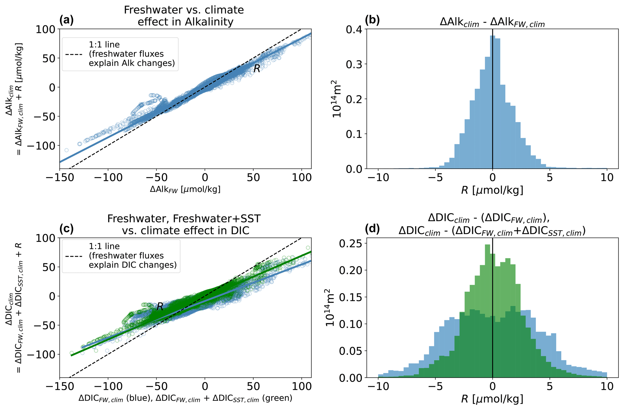
Figure A2 Ability of freshwater SST decomposition to reconstruct spatial pattern of changes in surface DIC and alkalinity with the climate effect. As in Fig. A1 but for the climate effect. The greater disagreement here is primarily due to anomalous fluxes.

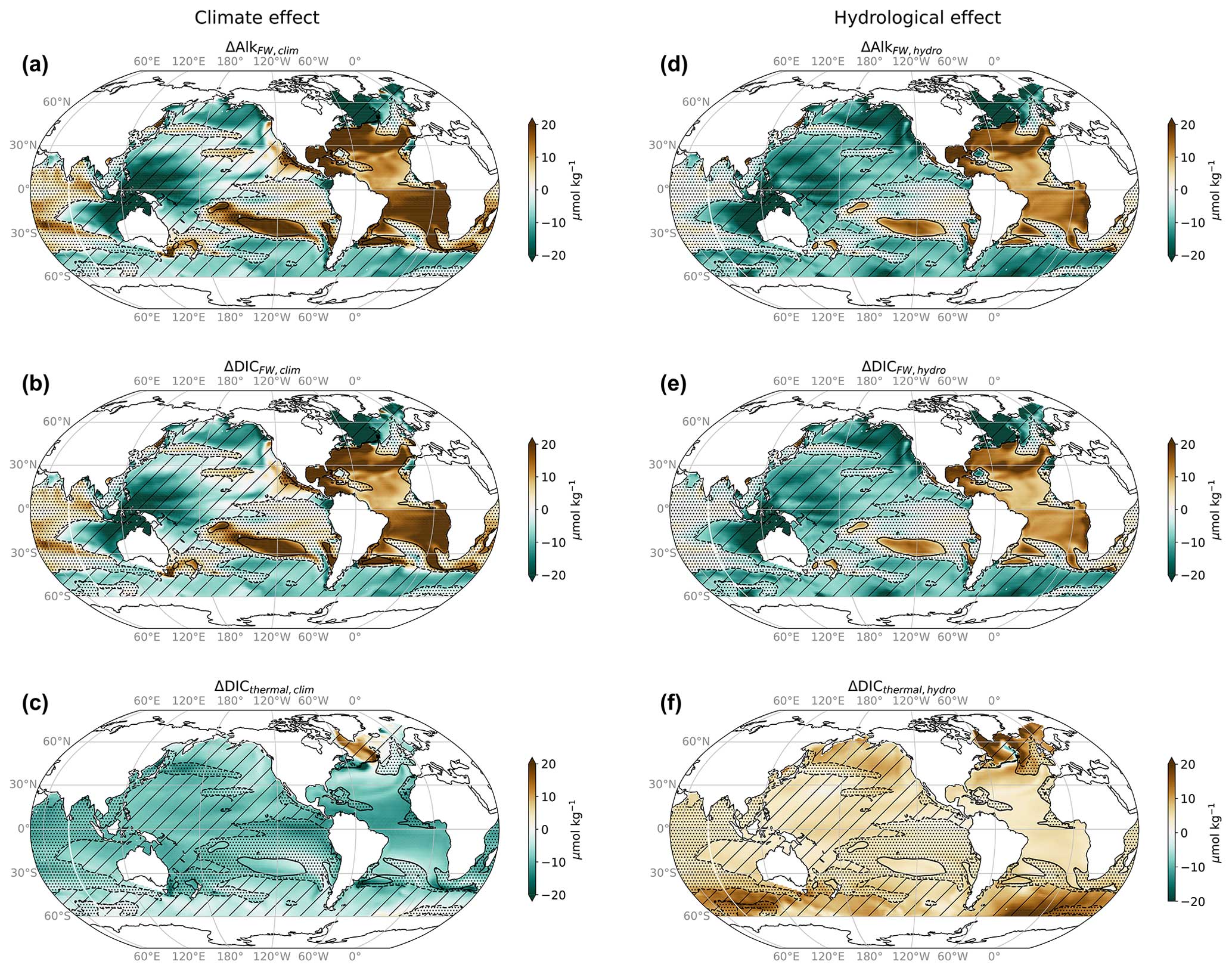
Figure A3 Thermal and freshwater components of DIC and alkalinity changes. (a–c) Change attributed to freshwater ($\mathrm{\Delta }{\text{Alk}}_{\mathrm{FW},\mathrm{clim}}=f_{\mathrm{FW},\mathrm{clim}}{\text{Alk}}_{\mathrm{Fix}\text{-}\mathrm{Clim}}$, $\mathrm{\Delta }{\text{DIC}}_{\mathrm{FW},\mathrm{clim}}=f_{\mathrm{FW},\mathrm{clim}}{\text{DIC}}_{\mathrm{Fix}\text{-}\mathrm{Clim}}$) and thermal ($\mathrm{\Delta }{\text{DIC}}_{\mathrm{thermal},\mathrm{clim}}=-\mathrm{7}\mathrm{\Delta }{\text{SST}}_{\mathrm{clim}}$) components in the climate effect; (d–f) change attributed to freshwater ($\mathrm{\Delta }{\text{Alk}}_{\mathrm{FW},\mathrm{hydro}}=f_{\mathrm{FW},\mathrm{hydro}}{\text{Alk}}_{\mathrm{Fix}\text{-}\mathrm{SSS}}$, $\mathrm{\Delta }{\text{DIC}}_{\mathrm{FW},\mathrm{hydro}}=f_{\mathrm{FW},\mathrm{hydro}}{\text{DIC}}_{\mathrm{Fix}\text{-}\mathrm{SSS}}$) and thermal ($\mathrm{\Delta }{\text{DIC}}_{\mathrm{thermal},\mathrm{hydro}}=-\mathrm{7}\mathrm{\Delta }{\text{SST}}_{\mathrm{hydro}}$) components in the hydrological effect.

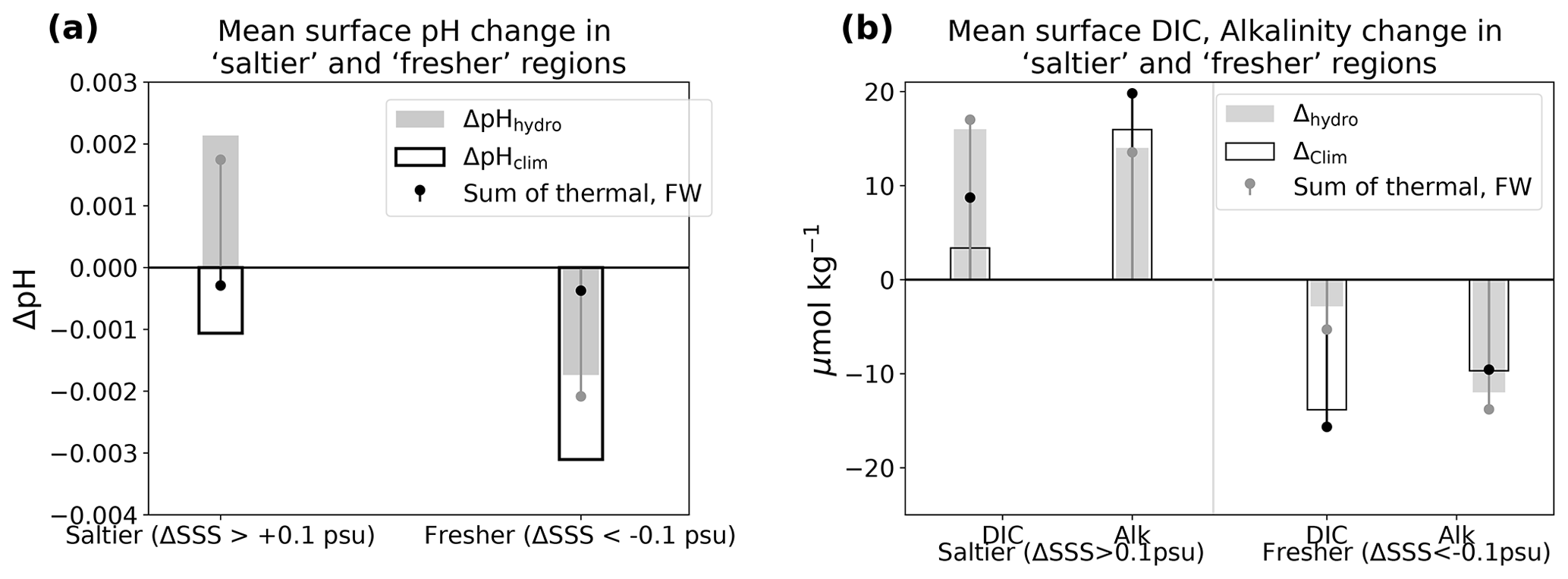
Figure A4 Error in our estimation of pH, DIC, and Alk changes, averaged over salty-get-saltier and fresh-get-fresher regions. Bars of pH change in panel (a) are identical to those in Fig. 4c, while bars of DIC and Alk change in panel (b) are identical to those in Fig. 2e (i.e., empty black bars correspond to the climate effect, while the grey filled bars correspond to the hydrological effect). Lollipops make a comparison between the estimate from our decomposition and the full changes simulated by ESM2M (represented by the bars). Grey lollipops represent $\mathrm{\Delta }{X}_{\mathrm{FW},\mathrm{Hydro}}+\mathrm{\Delta }{X}_{\mathrm{thermal},\mathrm{Hydro}}$ (X is pH, DIC, or Alk), and the difference between the grey bars and lollipops is R_Hydro. Black lollipops represent $\mathrm{\Delta }{X}_{\mathrm{FW},\mathrm{Clim}}+\mathrm{\Delta }{X}_{\mathrm{thermal},\mathrm{Clim}}$ (X is pH, DIC, or Alk), and the difference between the black bars and lollipops is R_Clim. Please see Sect. 2 and Tables 2 and 3 for calculations of FW and thermal components of pH, DIC, and Alk.

Figure A5 Air–sea flux of CO₂: difference due to (a) climate effect and (b) hydrological effect. Stippling denotes where ΔSSS_hydro is small, as in Figs. 1, 2, 4, and 5.