the Creative Commons Attribution 4.0 License.
the Creative Commons Attribution 4.0 License.
 | 29 Jan 2024
Microclimate mapping using novel radiative transfer modelling
Florian Zellweger
Eric Sulmoni
Johanna T. Malle
Andri Baltensweiler
Tobias Jonas
Niklaus E. Zimmermann
Christian Ginzler
Dirk Nikolaus Karger
Pieter De Frenne
David Frey
Clare Webster
Climate data matching the scales at which organisms experience climatic conditions are often missing. Yet, such data on microclimatic conditions are required to better understand climate change impacts on biodiversity and ecosystem functioning. Here we combine a network of microclimate temperature measurements across different habitats and vertical heights with a novel radiative transfer model to map daily temperatures during the vegetation period at 10 m spatial resolution across Switzerland. Our results reveal strong horizontal and vertical variability in microclimate temperature, particularly for maximum temperatures at 5 cm above the ground and within the topsoil. Compared to macroclimate conditions as measured by weather stations outside forests, diurnal air and topsoil temperature ranges inside forests were reduced by up to 3.0 and 7.8 ∘C, respectively, while below trees outside forests, e.g. in hedges and below solitary trees, this buffering effect was 1.8 and 7.2 ∘C, respectively. We also found that, in open grasslands, maximum temperatures at 5 cm above ground are, on average, 3.4 ∘C warmer than those of the macroclimate, suggesting that, in such habitats, heat exposure close to the ground is often underestimated when using macroclimatic data. Spatial interpolation was achieved by using a hybrid approach based on linear mixed-effect models with input from detailed radiation estimates from radiative transfer models that account for topographic and vegetation shading, as well as other predictor variables related to the macroclimate, topography, and vegetation height. After accounting for macroclimate effects, microclimate patterns were primarily driven by radiation, with particularly strong effects on maximum temperatures. Results from spatial block cross-validation revealed predictive accuracies as measured by root mean squared errors ranging from 1.18 to 3.43 ∘C, with minimum temperatures being predicted more accurately overall than maximum temperatures. The microclimate-mapping methodology presented here enables a biologically relevant perspective when analysing climate–species interactions, which is expected to lead to a better understanding of biotic and ecosystem responses to climate and land use change.
- Article
(14098 KB) - Full-text XML
- BibTeX
- EndNote


Current understandings of climate and climate change impacts on biodiversity and ecosystem functioning are often based on macroclimate data available at spatial scales much coarser than the microclimatic conditions experienced by organisms (Bramer et al., 2018; Potter et al., 2013). Most of these macroclimate datasets are based on interpolations of standardized weather station data, typically using temperature measurements taken outside of forests and above grasslands at ∼ 2 m above ground level. However, across landscapes, local topography and vegetation cover create heterogeneous microclimates through altering local radiation regimes, air mixing, and evapotranspiration. Macroclimate data are therefore limited in representing near-surface microclimate conditions close to or in the ground and under vegetation canopies where most terrestrial organisms reside. Given the importance of microclimates for the physiology of organisms, as well as for key ecosystem processes such as carbon, nutrient, and water cycling, accurately predicting microclimates at high spatial and temporal resolutions is fundamental for understanding climate and climate change impacts on biodiversity and ecosystem functioning (Jones, 2014; De Frenne et al., 2021).
Variation in microclimate is driven by the topography, vegetation, soil, and the water balance, all of which modulate near-surface temperatures in relation to the prevailing macro-scale meteorological conditions (Geiger et al., 2009). Local controls on microclimates include the buffering of forest understories against macroclimate temperature extremes (De Frenne et al., 2019; Chen et al., 1999) and the high heterogeneity of surface microclimates in topographically complex environments, such as mountains (Scherrer and Körner, 2010). For example, maximum temperatures and temperature extremes can be reduced in areas shaded by topography and/or vegetation due to the reduction in incoming shortwave solar radiation, an effect that can be increased by evapotranspirative cooling if water availability is not limited (De Frenne et al., 2021). Minimum temperatures, on the other hand, are modulated by factors such as heat retention by vegetation canopies through reduced outgoing longwave radiation and reduced wind speeds, as well as cold air flow and pooling in topographic depressions, particularly during the night and calm atmospheric conditions (Dobrowski, 2011; Geiger et al., 2009).
Fortunately, mapping of microclimates has recently been facilitated by advanced microclimate measuring and modelling techniques (Maclean et al., 2018; Zellweger et al., 2019a; Maclean et al., 2021) and the compilation of large databases of in situ microclimate measurements (Lembrechts et al., 2020). These new data streams and technologies are now being used to create large-scale microclimate datasets and mapping products that will contribute to a better understanding of the climate-related distribution and functioning of organisms (Lembrechts et al., 2019b; Suggitt et al., 2018; Maclean and Early, 2023; Haesen et al., 2023a; Lembrechts et al., 2022).
Mapping microclimate across landscapes has particularly been assisted by remote sensing technologies such as light detection and ranging (lidar) and digital photogrammetry, which provide detailed information about the topography and vegetation structure that can be used as input variables to model near-surface temperatures (Jucker et al., 2018; Frey et al., 2016; Duffy et al., 2021; Greiser et al., 2018; Maclean et al., 2018). A key challenge in microclimate mapping is incorporating radiation transfer through vegetation canopies, which has often been crudely represented via the use of canopy cover and density proxies such as leaf area index (LAI), canopy height, and/or canopy cover. These proxies lack the directional component in relation to radiation transfer and typically generalize the canopy away from the individual tree-level structure, both of which impact the physiology of organisms. Using these proxies can therefore lead to errors in estimates of canopy transmissivity in heterogeneous forest canopies (Musselman et al., 2013), thereby increasing uncertainties for analysing microclimate effects on plant species composition (Zellweger et al., 2019b). Newer mechanistic microclimate models are now able to account for radiative transfer through canopies, as well as attenuation of wind speed (Maclean and Klinges, 2021), and specific radiative transfer models based on remotely sensed 3D vegetation structure datasets accurately calculate canopy transmissivity maps at metre- and even sub-metre-scale resolution by directly accounting for detailed and realistic canopy structure in relation to the changing daily and seasonal solar position (Musselman et al., 2013; Bode et al., 2014; Tymen et al., 2017; Webster et al., 2020; Kükenbrink et al., 2021; Webster et al., 2023). Together with the increasing availability of 3D vegetation structure datasets at the tree level across large spatial extents, these developments enable the incorporation of detailed radiative transfer variables in microclimate-mapping approaches.
A further limitation to current microclimate analysis and mapping is the lack of reliable in situ microclimate measurements across a wide range of habitats. In places exposed to sunlight, for example, many commonly used microclimate temperature loggers – shielded or unshielded – record biased measurements due to radiative fluxes operating-on the thermometer (Maclean et al., 2021). Fortunately, these biases can now be minimized by using ultra fine-wire thermocouples with a low thermal emissivity and highly reflective surface, recording accurate estimates of air temperatures, even in places exposed to sunlight or close to the ground (Maclean et al., 2021). Deploying these measurement devices across multiple habitat types that span wide ranges of variation in vegetation structure and topography is thus required to arrive at a reliable reference dataset that is representative of the entire spectrum of microclimate conditions within environmentally heterogeneous regions. This would, for example, allow researchers to include the often ignored but specific thermal conditions beneath trees outside forests, e.g. in hedges, providing important habitats and increasing habitat connectivity in microclimate-mapping products (Vanneste et al., 2020).
Here we combine a state-of-the-art radiative transfer model with a comprehensive microclimate measurement network to infer and map daily microclimate temperatures at three vertical heights and 10 m spatial resolution across the whole of Switzerland. The resulting microclimate dataset is a major step forward towards taking a realistic organism's perspective when studying species–climate interactions and will be relevant to many fields of biological and environmental sciences, including fundamental and applied ecology, hydrology, agriculture, and forestry (De Frenne et al., 2021; Bramer et al., 2018).
2.1 Study area
This study was carried out in Switzerland, which covers 41 248 km2 of central Europe. Mountains cover ca. 70 % of the country, and lowlands cover the remaining 30 %. One-third of the land is forested, with a larger proportion in the mountain areas. The forest composition consists of coniferous (42 %), mixed (34 %), and deciduous (24 %) forests (Brändli et al., 2020); 4 % of the country (1813 km2) is covered by trees outside of forests, e.g. trees found in hedges or solitary trees (Malkoç et al., 2021).
2.2 Temperature measurements inside and outside forests
We implemented a nationwide network of microclimate temperature sensors following a hierarchical stratified sampling design. First, we identified eight regions to represent the main macroclimate gradients in Switzerland (Fig. 1). These regions align with the long-term Forest Ecosystem Research (LWF) network, covering gradients ranging from the lowlands with a temperate, relatively warm climate to higher and cooler elevations receiving more precipitation to inner alpine regions with a continental climate and regions in the southern Alps with an insubric climate. In each region, we installed temperature sensors in several plots, covering the regional variation in forest structure and topography. Inside forests, we identified locations with low to high topographic slope angles and topographic positions, as well as locations with different slope orientations, i.e. from north- to south-facing slopes. In each of the forest locations, we sampled one plot with high canopy cover and one plot with low canopy cover, as visually estimated in the field. All forest plots were at least 50 m away from the nearest forest edge. Outside forests, we sampled grasslands with different slope orientations, as well as high and low relative topographic positions, i.e. ridges to valley bottoms. Finally, in each region, we selected plots below trees outside forests. In hedge-type habitats, i.e. linear accumulations of woody vegetation, we placed the loggers in the middle of each hedge. Below solitary trees, we placed the loggers at half the distance between the tree trunk and outer crown projection line. Due to regional plot availability and suitability as determined by field visits, the number of final plots per region varied, ranging from 6 to 17 (median of 15) plots per region. The total number of plots was 107, with 62 plots in forests, 22 below trees outside forests, and 23 in open grasslands. In the Pfynwald and southern Ticino, only forest plots were sampled. Our sample plots represented the observed range of environmental conditions across the study area well, as indicated by a comparison between sampled and observed predictor variable space across the area used for making predictions (Table B1 in the Appendix).
In each plot, microclimate temperatures were measured at 1 and 5 cm above the ground surface, as well as below the ground in the topsoil at 5 cm depth. These heights were chosen because we expect a large degree of vertical temperature variation between these heights, as indicated by common temperature profiles (De Frenne et al., 2021) and because these heights are representative of the strata in which many organisms reside (e.g. herbaceous plants, tree seedlings, ground arthropods, soil fungi, and bacteria). We acknowledge that sampling entire vertical forest profiles reaching the top tree canopy would be desired from an ecological viewpoint, but we were not able to achieve this due to logistic reasons. Above-ground air temperatures (both at 1 m and 5 cm) were recorded hourly using Lascar Electronics EL-USB-TC loggers with unshielded ultra-fine-wire thermocouples (0.08 mm) taped to a 1 m tall fencing pole (Fig. 1d–e). For sampling at 5 cm below the ground, we used standard Lascar EL-USB-1 loggers placed into a buried, small, sealable plastic tube, also recording at an hourly resolution. Both the thermocouples and standard Lascar logger types have a measuring accuracy of 0.3 ∘C, as reported by Lascar Electronics. To check if the measurements of the unshielded thermocouples were affected by direct sunlight we performed an experimental sensitivity test, which revealed no significant effect of direct sunlight (Appendix A). The measurement period started on 8 June 2021 and ended on 31 October 2022, with slightly varying starting dates per region as determined by the site visits to install all loggers. The sampling duration was thus long enough to include a wide range of weather conditions, from wet and cold to hot and dry periods. All sites were revisited every 2 to 3 months for maintenance and to retrieve the data. Together with careful checks and corrections for obvious outliers and data artefacts introduced by device malfunction or disturbance by animals, this maintenance enabled us to build up a mostly seamless time series of hourly temperature data, with an overall loss of data of less than 5 %. Each site was georeferenced using a Trimble® GeoExplorer 6000 with an accuracy after post-processing of ca. 1 m.
For the analysis presented here we pooled all data collected between June 2021 to October 2021 and April 2022 to October 2022, broadly representing the vegetation periods observed across Switzerland. We further excluded all temperature recordings that were made under snow cover, which mainly affected the measurements 5 cm above ground and 5 cm below ground at high elevations. We did this because snow blankets introduce spatial and temporal variability of atmospheric decoupling in temperatures below or within a snow blanket, and this variability cannot accurately be modelled with our predictor variables.
To build the final time series dataset for the spatial modelling we aggregated the hourly data to daily maximum (Tmax micro), mean (Tmean micro), and minimum (Tmin micro) temperature. Tmax micro was defined as the 24 h 95th percentile, and Tmin micro was defined as the 5th percentile. Tmean micro is the arithmetic daily mean temperature (with n=24). These three daily temperature statistics are the dependent variables for the models used to predict nationwide microclimate temperature maps as outlined below.
To analyse the differences between the microclimate and macroclimate data, i.e. the microclimate variation not captured by macroclimate data, we computed the temperature offsets (De Frenne et al., 2021) as the macroclimate temperature minus the microclimate temperature (see section “Predictor variables” for details). Temperature offsets were thus only used to quantify the observed difference between the micro- and macroclimate, while the spatial modelling was based on the actual microclimate temperatures measured.
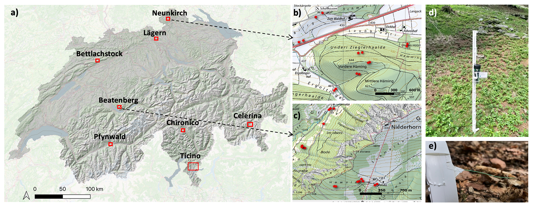
Figure 1Sampling design for microclimate-measuring network across Switzerland. (a) Distributions of the eight regions spanning a wide macroclimatic gradient across the country. In each region, sites were identified to represent regional variation in vegetation structure and topography (see text for details); (b) and (c) are the distribution of sites in the regions of Neunkirch and Beatenberg, respectively (© swisstopo). (d) Installation of microclimate sensors, with an ultra-fine-wire thermocouple measuring the temperature 5 cm above the ground, as shown in (e).
2.3 Predictor variables
The development of our predictor variable set was guided by the assumption that the variation in near-surface microclimate temperatures, as measured by our sensor network, is strongly related to variation in macroclimate temperature, followed by the effects of local-scale variation in topography, vegetation structure, and associated radiation regimes.
To derive the macroclimate we used interpolated daily maximum Tmax Macro, daily mean Tmean Macro, and daily minimum Tmin Macro data from meteorological stations as provided by MeteoSwiss at a 1 km2 nationwide grid (Frei, 2014). The underlying data for these macroclimate layers were collected at 131 weather stations at 2 m height above ground in open localities outside forests across the country. For model fitting, as well as for the final predictions, we needed to downscale the 1 km2 macroclimate data to our 10 m target resolution, which was guided by the resolution of our other predictor variables, especially those describing the topography and vegetation height as described below. To this end we applied a lapse rate correction to the macroclimate layers, which is important in our mountainous study area, where the pronounced altitudinal gradients and related lapse rates cause large temperature differences within an original 1 km2 grid cell. Daily lapse rates were calculated for each Tmax macro, Tmean macro, and Tmin macro separately using a moving-window regression based on the respective 1 km2 temperature grid cell and the corresponding 1 km2 MeteoSwiss reference digital terrain model (DTM) with a moving 3×3 window size. We thus estimated, for each window, how much the temperature changes as a function of the regional elevation gradient. The resulting regression estimate is the daily lapse rate Γ (in ∘C m−1). Only grid cells with regression results with an R2>0.85 were considered to ensure a reliable lapse rate value. Remaining-empty raster cells were filled in a second step with the average lapse rate within a moving window of 5×5 cells. Based on visual inspection of the resulting lapse rate maps, this combination of window sizes resulted in the best achievable estimation of locally prevailing lapse rate values. The result of this process was nationwide 1 km2 resolution auxiliary maps of daily lapse rates for each Tmax macro, Tmean macro, and Tmin macro. The processing workflow is illustrated in Fig. G1 in Appendix G.
For the downscaling to the target resolution, the 1 km grids of both the lapse rate and the 1 km2 MeteoSwiss Tmax macro, Tmean macro, and Tmin macro rasters were first resampled to 10 m resolution with bilinear interpolation. Then, the 10 m MeteoSwiss daily Tmax macro, Tmean macro, and Tmin macro maps were corrected for sub-grid elevation variability using the 10 m lapse rate information as follows:
where Δz is the difference between each 10 m grid cell of Swissalti3D DTM elevation zDTM (Swisstopo, 2020) and the nearest 1km grid cell of the MeteoSwiss reference elevation for the temperature grids zMeteoSwiss. Tmax macro org, Tmean macro org, and Tmin macro org are the resampled 10 m MeteoSwiss temperature rasters, and Γ refers to the respective temperature lapse rates. The resulting lapse rate corrected daily macroclimate air temperature maps at 10 m resolution; i.e. Tmax macro cor, Tmean macro cor, and Tmin macro cor were used as predictor variables for the modelling and mapping of microclimate temperatures as measured within our network of microclimate temperature loggers (see the section “Microclimate modelling” below).
We also tested for the effects of daily cloud cover by incorporating actual macroclimate global radiation as derived from MeteoSwiss and found that daily cloud cover did not improve the predictive performance of our models, possibly because daily macroclimate temperatures already incorporate daily weather effects.
2.3.1 Radiative transfer model: shortwave transmissivity, sky view fraction, and subcanopy radiation
Small-scale variability in radiation within forests was represented by accounting for explicit tree-level forest structure around each point. Variability in the diffuse shortwave and longwave radiation components was represented using the 180∘ sky view fraction (Vf, also known as diffuse transmissivity). Variability in the direct shortwave component was accounted for by determining the proportion of the solar disc obscured by vegetation or topography (also known as time-varying direct-beam transmissivity, τdir), which varies both in space and in time as the solar position changes in the sky. Direct-beam transmissivity and sky view fraction were both calculated using the model CanRad (Webster et al., 2023), which uses synthetic 180∘ hemispherical images to replicate the topography and vegetation as seen by the ground or plant surface (Fig. 2). The radiation transfer model simulations represent only leaf-on conditions, which implies – contrarily to direct-beam transmissivity – that sky view fraction varies spatially but is temporally static. To resolve the fine-scale temporal variability of direct-beam transmissivity we calculated it at 2 min intervals and then averaged it to hourly time steps. CanRad was run at the point scale at 20 m intervals across the entire domain, totalling 87 795 419 points and 265 320 time steps across the annual solar cycle.
At all points, terrain shading was included by using 5 and 25 m DTMs (Swisstopo, 2020). The 5 m DTM was included up to a 300 m radius from each point to represent local terrain variability around each model point. The coarser 25 m DTM was used up to a 10 km radius from each point to calculate the topographic horizon line, accounting for terrain shading from nearby mountains.
For the above radiative transfer modelling we used the module C2R (CanopyHeightModel2Radiation) within CanRad, which achieves a realistic representation of the overhead canopy structure based on a canopy height model (CHM) to determine the geometric arrangement of vegetation surrounding a point, with information on forest type and subsequent leaf area of the individual tree crowns. The CHM was available at 1 m resolution based on lidar datasets ranging from 1 to 30 points m−2 acquired across Switzerland from 2012–2021, with one region (i.e. Pfynwald) having older data from 2003. The high spatial resolution of the CHM across the model domain ensured that the effects of individual trees on ground surface shading were explicitly incorporated. Forest type information was provided by the nationwide forest mix rate dataset from Waser et al. (2017) to discriminate between deciduous and evergreen forest types, and the Swiss forest ecoregions dataset (FOEN, 2022) was used to distinguish between needleleaf or broadleaf forest types. For a more thorough description of the radiative transfer modelling, see Webster et al. (2023).
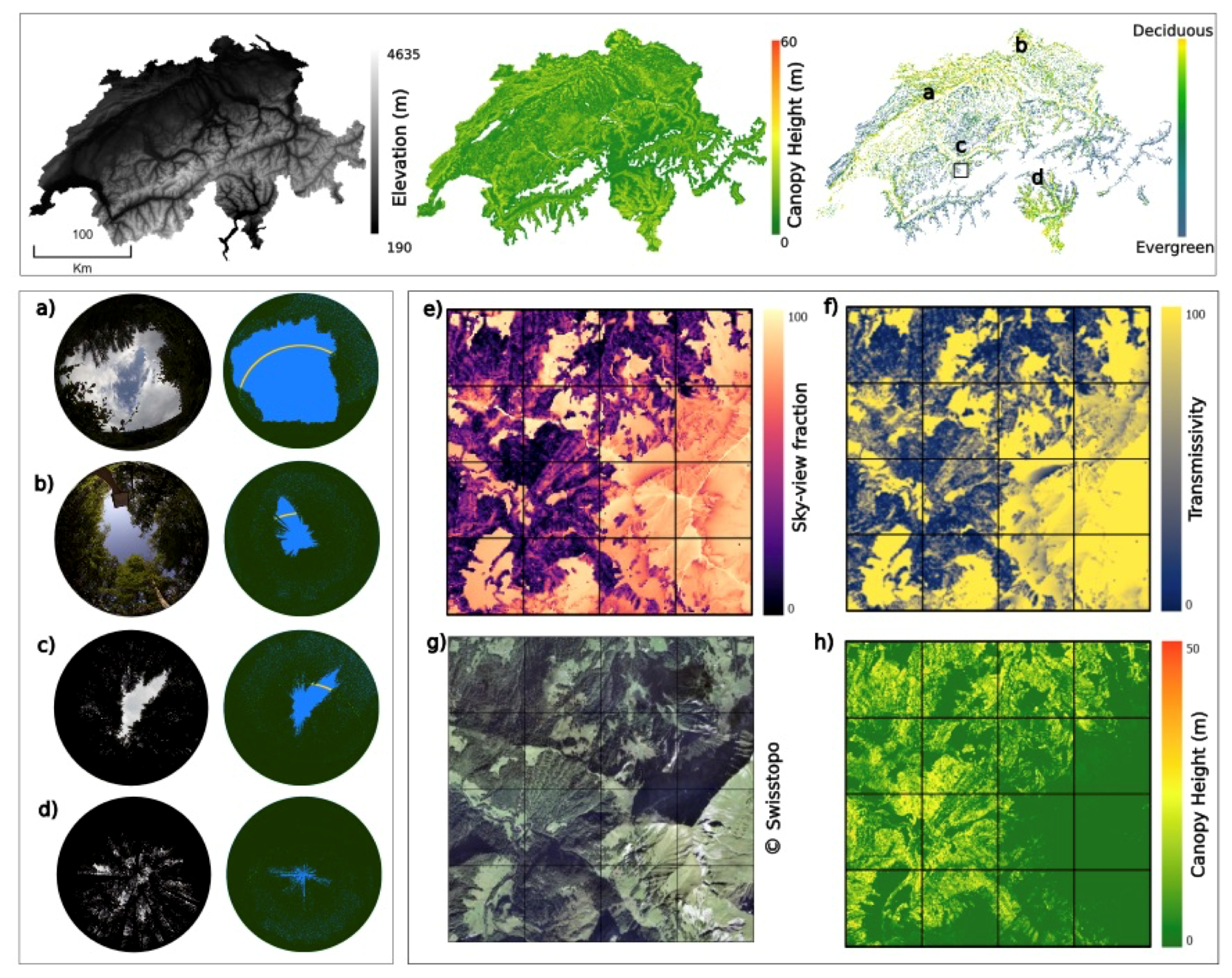
Figure 2Top: nationwide input datasets used in CanRad to calculate synthetic hemispherical images – elevation (left), canopy height (middle), forest type mix rate, and locations of outputs shown in bottom panels (right). Bottom left: examples of hemispherical photographs and corresponding synthetic images at the same locations. (a) Below shrubs, (b) deciduous broadleaf forest, (c) northern alpine evergreen coniferous forest, (d) southern alpine evergreen coniferous forest. In the synthetic images the yellow line corresponds to the solar track on 22 June. Sky view fraction is then calculated as the ratio based on a non-linear weighting of the blue + yellow area relative to the total area. Bottom right: example of model estimates of sky view fraction (e) and average transmissivity for June (f) over a 4 km2 region in the central Alps, as indicated by the black square in top-right forest mix rate map. Aerial image (g) and canopy height (h) shown for context. Note that photographs in a–d have not been corrected for lens distortion compared to synthetic images which have an equiangular lens projection.
The hourly estimates of direct-beam transmissivity were aggregated to daily values by averaging the values each day between the hours of 09:00 and 16:00 CET. The assumption here was that the daily maximum microclimate temperature is mostly dependent on solar radiation within this time interval. These daily aggregates were averaged to monthly averages thereafter and resampled from 20 to 10 m resolution using bilinear interpolation. Finally, we multiplied these monthly average transmissivity values with monthly averages of daily clear-sky direct shortwave irradiation as estimated by (Zimmermann and Roberts, 2001), yielding what hereafter is referred to as the direct radiation proxy. Note that this proxy represents both the spatial and the seasonal variation in subcanopy direct shortwave radiation.
As an additional predictor variable, we also extracted vegetation height at 10 m resolution from the above-mentioned CHM.
2.3.2 Topographic position and wetness index
We used the swissalti3D DTM with a 10 m resolution to derive indices of topographic position (TPI) and wetness (TWI). TPI and TWI serve as indicators for cold-air flow and pooling, as well as exposure to wind, thus affecting near-surface temperatures (Ashcroft and Gollan, 2013; Daly et al., 2008). TPI, or relative elevation, is defined as the normalized difference between the elevation of a focal cell and the average elevation within a minimum radius (here zero) and a maximum radius (here 120 m). TWI describes the lateral water flow and was calculated as follows:
where a is the upslope catchment area, and tan b is the local slope in radians (Freeman, 1991).
2.3.3 Soil moisture and rain
Soil moisture has been shown to affect near surface temperatures, for example by lowering the buffering magnitude of forest floor temperatures compared to outside forest temperature under dry conditions (von Arx et al., 2013). To account for the potential effects of soil moisture and precipitation on our measured microclimate temperatures we calculated a predictor variable termed rain sum using daily precipitation data from MeteoSwiss on a 1 km grid. To calculate this variable for each day (i.e. at a daily resolution) we summed up the precipitation over the preceding 30 d, giving a linearly decreasing weight to values further in the past.
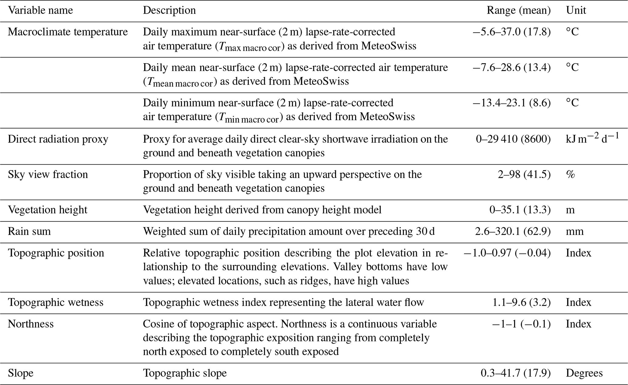
Table 1Predictor variables used for modelling, with the range of values representing the variable ranges across our microclimate sampling plots.
2.4 Microclimate modelling
We statistically related the plot-level measurements, i.e. the daily Tmax micro, Tmean micro, and Tmin micro measurements at different vertical heights, to the predictor variables (Table 1) and used the resulting model equations to predict national maps of daily microclimate over the entire gridded domain. The sample sizes for the 1 m, 5 cm, and topsoil datasets were , , and , respectively. As mentioned above, please note that our dependent variables were the actual microclimate temperature measurements and not the temperature offsets. We tested three modelling approaches to analyse the predictive performance of our predictor variables.
First, we fitted linear mixed-effect models with our predictor variables as fixed effects and region as a random intercept term to account for the non-independence among replicates from the same region using restricted maximum likelihood in the lmer function from the lme4 package in R (Bates et al., 2015). All variables were standardized, i.e. rescaled to have a mean of zero and a standard deviation of 1, to increase the interpretability of relative-effect sizes among the predictor variables. For Tmax micro and Tmean micro we included the interaction term between the macroclimate temperature and the direct radiation proxy at ground level and below canopy as it has been shown that the maximum temperature-buffering capacity of tree canopies can increase with warmer temperatures (De Frenne et al., 2019). Tmin micro was modelled as a function of sky view fraction instead of direct radiation to account for the negative net longwave radiation during the night as a presumed main driver of Tmin micro.
The second approach was a random forest regression model, using the randomForest package in R (Liaw and Wiener, 2002). Two variables were randomly sampled as candidates at each split, with a total number of 500 trees following conventions. We used this machine learning algorithm because it automatically considers variable interactions and non-linear relationships between dependent and independent variables. These features may lead to increased predictive accuracy because such interactions and non-linear relationships may indeed be present in our data as it has been shown that the effects of vegetation structure and topography on near-surface temperatures may be non-linear (Zellweger et al., 2019c).
To further test for non-linear responses, we also used general additive mixed-effect models (GAMMs) as our third modelling approach, applying the gamm function in the mgcv package in R (Wood, 2017). We again added region as a random term and used REML as the smoothing parameter estimation method for the model.
To evaluate the predictive performance of our models we applied a spatial block cross-validation approach and computed the R2 values and root mean squared errors (RMSEs) (Roberts et al., 2017). We therefore iteratively used data from seven out of the eight regions for model fitting and predicted the data from the left-out eighth region to compare the predicted with the observed values.
As indicated in the Results section, we used the linear mixed-effect models to produce daily microclimate maps across Switzerland at 10 m resolution covering the period between 1 April and 31 October for all the years between 2012 to 2021. We calculated these maps for daily Tmax micro, Tmean micro, and Tmin micro, each at 1 m and 5 cm above ground, as well as in the topsoil 5 cm below ground. As noted, these data are representative for snow-free conditions during the vegetation period and leaf-on conditions. The 10-year period has been chosen in acknowledgement of the fact that changes in tree cover and density do occur, where most of our lidar data used for the radiation modelling were acquired during the years 2012–2021. Because we have sampled microclimate data in neither urban areas nor settlements nor in non-vegetated areas, such as scree or glacial habitats, we masked those areas out from our microclimate maps using the land-cover-mapping product Vector25 (Swisstopo, 2022).
3.1 Temperature offsets in different habitats
The temperature offsets describe the differences between the microclimate and macroclimate data and thus indicate microclimate variation not captured in macroclimate data. Our nationwide sampling in different habitats revealed strong horizontal and vertical variability in temperatures during the vegetation period, with a particularly high degree of variation in daily maximum near surface and topsoil temperature measured at 5 cm above ground (5th and 95th percentiles: −4.6 and 8.2 ∘C) and 5 cm below ground (5th and 95th percentiles: −10.3 and 2.2 ∘C), respectively (Fig. 3). Daily temperature extremes as measured by Tmax micro and Tmin micro were considerably reduced in the topsoil and in forests, as indicated by negative offset values for Tmax micro and positive offset values of Tmin micro.
In forests, the daily Tmax micro were cooler than the daily Tmax macro outside forests, with mean offset values of −1.3 and −1.1 ∘C for air temperature at 1 m and 5 cm above ground, respectively, and −5.2 ∘C in the topsoil (Table C1). Daily Tmin micro were generally warmer, with average offset values of 1.8, 1.7, and 2.6 ∘C at 1 m and 5 cm above ground and in the topsoil, respectively. In forests, the resulting absolute differences between Tmax and Tmin offsets, i.e. the total temperature buffering effect, were thus 3.0, 2.9, and 7.8 ∘C, respectively.
Below trees outside forests we also found reduced daily extreme temperatures as compared to Tmax macro, but the magnitude of the temperature-buffering effect was lower than in forests. Daily Tmax micro were, on average, lower by −0.7, −0.2, and −4.9 ∘C at 1 m and 5 cm above ground and in the topsoil, respectively, while daily Tmin micro were, on average, higher by 1.1, 0.9, and 2.3 ∘C. The resulting total temperature-buffering effect below trees outside forests was thus 1.8, 1.1, and 7.2 ∘C, respectively.
Unlike in forests and trees outside forests, temperature offsets for maximum air temperatures at 5 cm in grasslands were found to be positive, i.e. 3.4 ∘C, indicating that near-surface Tmax micro in open habitats are often underestimated when using macroclimate data. Moreover, topsoil Tmin micro in open grasslands were warmer than the macroclimate by 3.5 ∘C on average. Across all habitat types we found that the degree of variation in offset values, particularly Tmax micro offset values, was greater at 5 cm above ground than at 1 m or in the topsoil, suggesting a high spatial variability in near-surface air temperatures across and within the different habitat types.
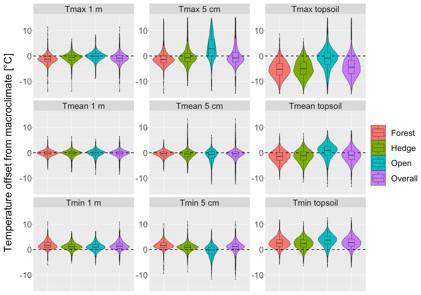
Figure 3Offsets between macroclimate and in situ measured microclimate temperature during April to October per habitat type and overall data points. The offsets were calculated by subtracting the microclimate temperature from the lapse-rate-corrected macroclimate temperature (Tmacro−Tmicro). Negative offset values thus indicate cooler microclimates compared to the macroclimate and vice versa.
3.2 Model performance
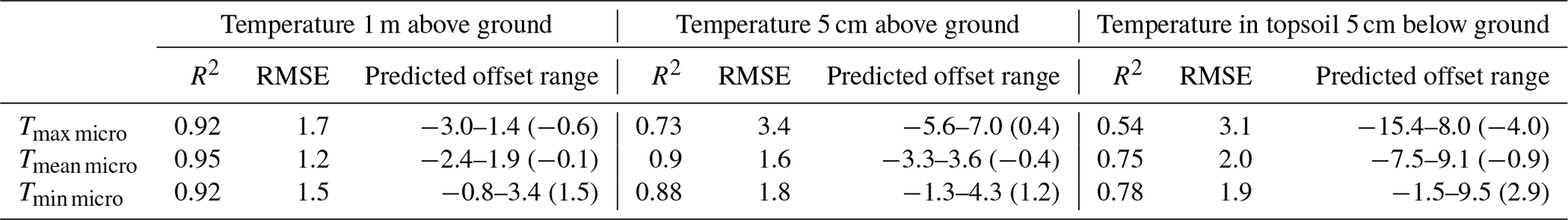
The predictive performance of our models ranged between R2 values of 0.54 and 0.95 and root mean squared errors (RMSEs) of 1.2 and 3.4 ∘C (Table 2, Fig. 4). Microclimate temperatures at 1 m height were predicted with the highest accuracy, followed by temperatures at 5 cm and in the topsoil. Tmin micro at 5 cm and in the topsoil were predicted considerably more accurately than the respective Tmax micro values. We also found large ranges in predicted temperature offsets, with generally wider ranges for Tmax micro than for Tmin micro. The widest range of offsets were found for topsoil Tmax micro, followed by Tmax micro at 5 cm and 1 m.
The observed patterns in model performance and predicted offset value ranges were broadly similar across the three tested modelling approaches, but it is noteworthy that random forests, as well as GAMMs, predicted considerably larger offset ranges (Table D1). Yet, when evaluated based on block cross-validation, linear mixed-effect models had the highest overall predictive skill. We thus used the linear mixed effects models to evaluate individual predictor variable effects and to calculate the final microclimate maps.
We also compared the predictive performance of our microclimate models against a model using macroclimate predictor variables only. This analysis confirmed the expectation that, given the broad macroclimatic gradients in our study and the period analysed (i.e. April–October), most of the variance is explained by the macroclimate (Appendix E).
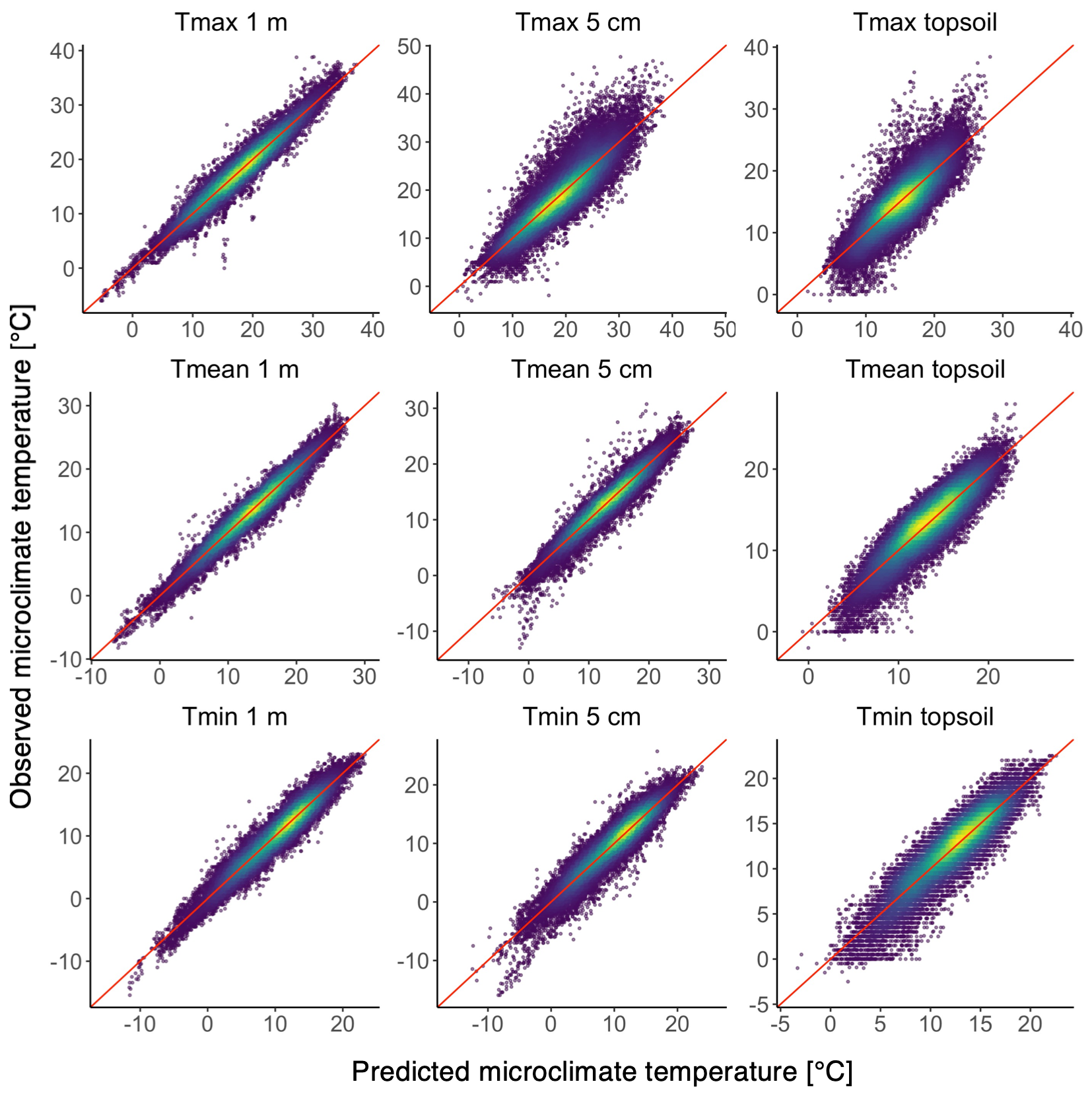
Figure 4Predicted versus observed plots showing predictions from linear mixed-effects model. The sample density is indicated by the colour scale, with yellow showing highest sample densities; the red line represents the 1:1 relationship.
Table 2Predictive performance of linear mixed-effect models, quantified using block cross-validation. We also report the predicted offset ranges, i.e. minimum to maximum, and mean in brackets, calculated as the difference between the predicted microclimate and the macroclimate.
3.3 Predictor variable effects
In line with the expectation that microclimate patterns broadly follow macroclimate dynamics we found that macroclimate variables had the strongest effects on the microclimate, as indicated by the highest standardized variable estimates (Fig. 5). Yet, most of the predictor variables related to radiation, vegetation, and topography significantly modulated the local variation of microclimate.
We found that Tmean micro and Tmax micro were strongly related to direct radiation, with particularly large effects on Tmax micro at 5 cm above ground and in the topsoil 5 cm below ground. The interaction effects between the macroclimate and direct radiation were relatively weak but significant. Specifically, the effect of direct radiation increased with increasing Tmax macro for Tmax micro at 1 m and 5 cm, but the opposite was true for Tmean micro. Sky view fraction strongly modulated Tmin micro, with negative effects on Tmin micro at 1 m and 5 cm, and positive effects on topsoil Tmin micro. Vegetation height had the largest effects on Tmax, cooling down Tmax micro as vegetation height increased across all three measurement heights. Higher water availability as estimated by the rain sum of the preceding 30 d generally had a small but significant cooling effect on microclimate temperatures at 1 m and 5 cm and a warming effect on topsoil temperatures. From all topography variables tested, topographic wetness and northness had the largest effects, predominantly cooling temperatures across all three heights at higher levels of topographic wetness and northness. In general, radiation and the vegetation height affected microclimate temperatures more strongly than variables related to water content and topography.
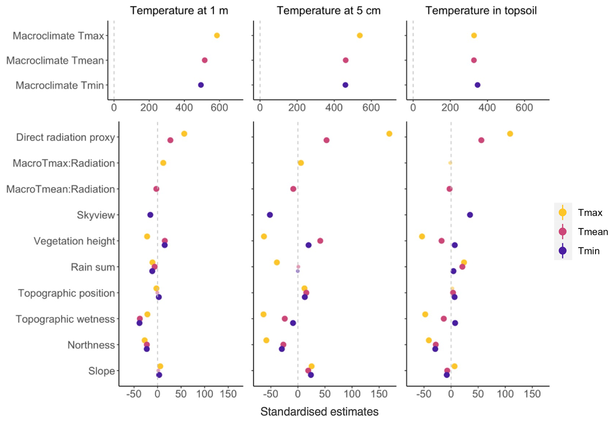
Figure 5Standardized model coefficient estimates from linear mixed-effect models for daily microclimate temperatures at different vertical heights, i.e. at 1 and 5 cm above ground and 5 cm below ground. The estimates on the x axis indicate the standardized effect sizes and direction of each variable. Standard errors are indicated by error bars; however, due to the large sample size, the error bars are small and invisible. Small transparent dots indicate non-significant (p>0.05) relationships.
3.4 Microclimate maps
Our microclimate maps show pronounced differences compared to currently available macroclimate layers (Fig. 6). Spatial variation in microclimates is particularly evident between forest and non-forest areas, and microclimate effects of trees outside of forests, e.g. in hedges or similar linear tree habitats, become visible. The strongest vertical temperature differences emerge between topsoil and near-surface air temperatures. All daily maps of Tmin micro, Tmean micro, and Tmax micro for all three vertical heights have also been aggregated to monthly averages, which are publicly available (see “Code and data availability” section). The broad coverage in our model calibration data in terms of environmental variation led to hardly any predictions outside the model calibration data (Table B1), minimizing potential uncertainties related to extrapolation.
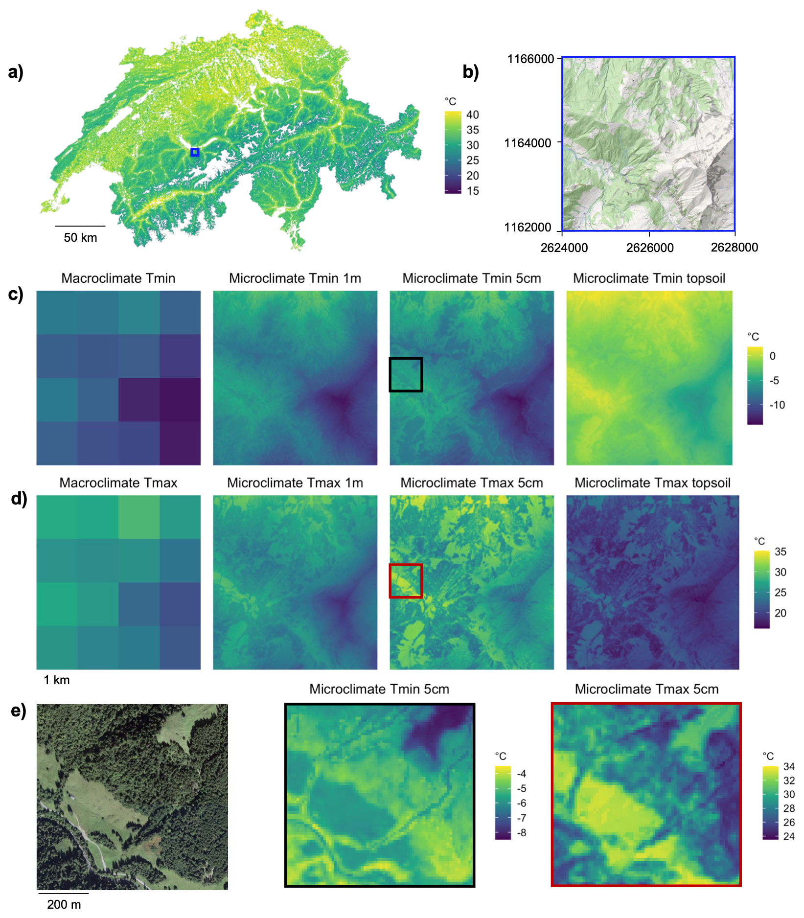
Figure 6Microclimate maps for Switzerland. (a) Nation-wide map of daily maximum microclimate temperature in summer; (b) 4×4 km hill-shaded sample region with forest cover shown in light green – the location of the region is indicated by a blue rectangle in (a). Across the sample region we illustrate our microclimate maps in comparison with the macroclimate data, with the maps in (c) representing the conditions on a frost day in spring and the maps in (d) showing the conditions on a warm summer day. (e) Shows a smaller area (coloured rectangles in c and d), illustrating the small-scale temperatures during a frost day in April 2021 and a warm summer day in July 2018. Source for macroclimate maps in (c) and (d): MeteoSwiss.
Our measured microclimate temperatures within an environmentally heterogeneous region revealed strong vertical and horizontal variation in near-surface temperatures. This microclimate variation can be mapped with high accuracy at a national scale, thus overcoming a prevalent limitation of macroclimate temperature maps that do not represent small-scale temperature variation. For example, our microclimate-mapping approach reveals the distribution of locations that experience substantially reduced daily temperature extremes, such as along-forest density gradients. The temperature-buffering effect was particularly pronounced for temperatures in the topsoil 5 cm below ground and air temperatures 5 cm above ground and less so for air temperatures 1 m above ground, a finding that aligns well with expected vertical temperature profiles in forests (De Frenne et al., 2021). The ability to map this temperature-buffering effect along a vertical temperature gradient is expected to provide crucial information to better understand microclimate–species interactions and their implications for biodiversity and ecosystem functioning (De Frenne et al., 2021; Lembrechts et al., 2019a).
Trees and shrubs have a strong impact on near-surface and topsoil temperatures, mainly via their effects on the radiation regime but also via their effects on wind speed and evapotranspiration (Geiger et al., 2009). We found a particularly strong positive effect of direct shortwave radiation on microclimate Tmax at 5 cm above ground and in the topsoil, implying that incoming radiation is the main controlling variable of ground-level microclimates once the macroclimate is accounted for. In line with the expectation that daily Tmin are higher under dense canopies because of longwave enhancement (Webster et al., 2016), we found a negative effect of sky view fraction on both above ground Tmin at both 5 cm and 1 m above ground. Topsoil Tmin, however, was positively affected by sky view fraction, potentially due to a higher degree of topsoil warming outside forests. These results imply that including high-resolution 3D remote sensing data of forest structure and derived radiation estimates significantly increase our capability to describe microclimatic variation.
Promising avenues for future microclimate modelling thus include the incorporation of temporarily dynamic data about forest cover and structure. Our detailed assessments of radiation effects on microclimatic variation relied on the application of a high-resolution radiative transfer model to estimate controls on radiation below the canopy considering the position and crown architecture of each tree in the landscape (Webster et al., 2023). Integrating this model into our microclimate-mapping approach constitutes an important novelty as it not only furthers more conventional approaches to estimate vegetation effects on radiation, e.g. via the use of light availability proxies such as canopy height, cover, or leaf area index (LAI), but also provides a pathway to quantify the effect of different natural and management-related forest dynamics on near-surface and topsoil temperatures. Such analyses now become feasible as the canopy structure information input into the radiative transfer model can be manipulated to represent past or future forest structure, where a subsequent model update would reveal the microclimatic impact quantitatively. Similar avenues are also provided by mechanistic microclimate models that incorporate physical processes more explicitly (e.g. Maclean and Klinges, 2021). These analyses are particularly relevant because it is increasingly evident that land use effects, e.g. from forest management practices but also from increased forest disturbances (e.g. due to droughts, bark beetles, wind storms) can have strong immediate effects on microclimate temperatures (Senf and Seidl, 2021), invoking microclimate temperature changes that are ecologically more relevant for explaining biodiversity dynamics than macroclimate change (Zellweger et al., 2020; Christiansen et al., 2022). Such approaches thus allows for including both past and future woody vegetation dynamics into the microclimate modelling, thus addressing an important methodological gap in microclimate science (De Frenne et al., 2021).
Another avenue for future microclimate modelling consists of comparing the relative strengths of statistical versus mechanistic models that are built based on physical processes. It would be interesting to incorporate the outputs of our radiative transfer model (e.g. sky view fraction and the proxy for direct radiation) into commonly used mechanistic models, e.g. NicheMapR (Kearney and Porter, 2017; Kearney et al., 2020) or microclimc (Maclean and Klinges, 2021), and to assess how well each approach performs in predicting microclimate time series given the different emphases on statistical and physical depiction. Performing this analysis at a high temporal resolution (e.g. hourly) would simultaneously allow us to assess how much the aggregation of our direct radiation proxy to daily vs. hourly values affects the added value of our detailed radiative transfer modelling.
We further found that microclimate temperatures were considerably reduced at locations with increased topographical wetness and northness, with relatively large effects on Tmax. These effects are expected to be related to generally cooler conditions in north-exposed places, as well as in places with large lateral, topographically derived water flow, e.g. via higher soil water content and cold-air flow. We further found that increases in rain sum, i.e. our variable indicative of soil moisture, resulted in lower Tmax at 5 cm above ground, confirming previous findings that soil moisture affects near-surface microclimates (von Arx et al., 2013). However, our results also show that the overall effect of the rain sum on topsoil and near-surface temperature was relatively weak.
The primary outputs of this work are maps of daily microclimatic temperatures during the vegetation seasons of the years 2012–2021. These maps improve some key scale limitations inherent in currently available macroclimate datasets; i.e. they improve on spatial scale by modelling microclimates at 10 m resolution while maintaining a daily temporal resolution, and they represent microclimates at three vertical heights – 1 m and 5 cm above ground and 5 cm within the topsoil – thus also improving upon vertical resolution. These improvements have a range of implications for future assessments of climate–species interactions and our understanding of climate change impacts on biodiversity. Species temperature preferences, microclimate heterogeneity, and microclimate refugia, for example, can now be mapped in much greater detail, which is expected to improve the accuracy of the analysis and forecasting of species distributions and range dynamics (Lembrechts et al., 2019b; Maclean and Early, 2023; Haesen et al., 2023b). The high resolution of our data also enables a more precise estimation of threshold-dependent temperature variables, such as degree days or frost frequencies, which is expected to improve models and approaches that depend on such variables, e.g. models of population dynamics or site suitability assessments for regenerating target tree species. In sum, these maps enable a more realistic, organism-centred perspective when analysing climate–species interactions and are thus relevant to both fundamental and applied ecology, as well as agriculture and forestry in the face of climate change.
Ultra-fine-wire thermocouples have been shown to accurately measure microclimate air temperatures and have outperformed shielded standard logger types in measuring air temperatures in locations exposed to direct sunlight or close to the ground, of which our sampling design contained many (Maclean et al., 2021). To test the potential effects of direct solar radiation on the thermocouples measurements we performed a shielding experiment. This experiment consisted of a paired design, where we placed two shielded and two unshielded thermocouples in each of the three representative environments for the field sampling (open, trees outside forest, and forest). The shields consisted of a lid of aluminium foil such that the thermocouple was just shaded but not isolated from wind (Fig. F1). The experiment was carried out during sunny conditions over 3 weeks in summer 2022. The analysis revealed overall RMSEs of 0.35 and 0.18 ∘C for daily maximum and mean temperatures between the shielded and unshielded thermocouples, both values being close to the measurement accuracy of 0.3 ∘C. We also did not find a significant difference between the three environments tested. This sensitivity analysis confirmed previous findings (Maclean et al., 2021) and shows that the effect of direct solar radiation on the thermocouples is negligible in our study setup.
Table B1Comparison of sampled predictor variable range and the observed predictor variable range across the entire area in relation to which predictions were made. Sampled range describes the predictor variables extracted at sampling plot locations; predicted range refers to the 1st and 99th percentiles of a random subset () of observed values across the predicted microclimate maps. Note that we did not include the macroclimate and rainsum variables in this table because they are dynamic variables with a daily resolution in our models, yet, as our sampled regions cover the observed macroclimate temperature and rainfall patterns across Switzerland well, we are confident that the sampled range matches the predicted range.
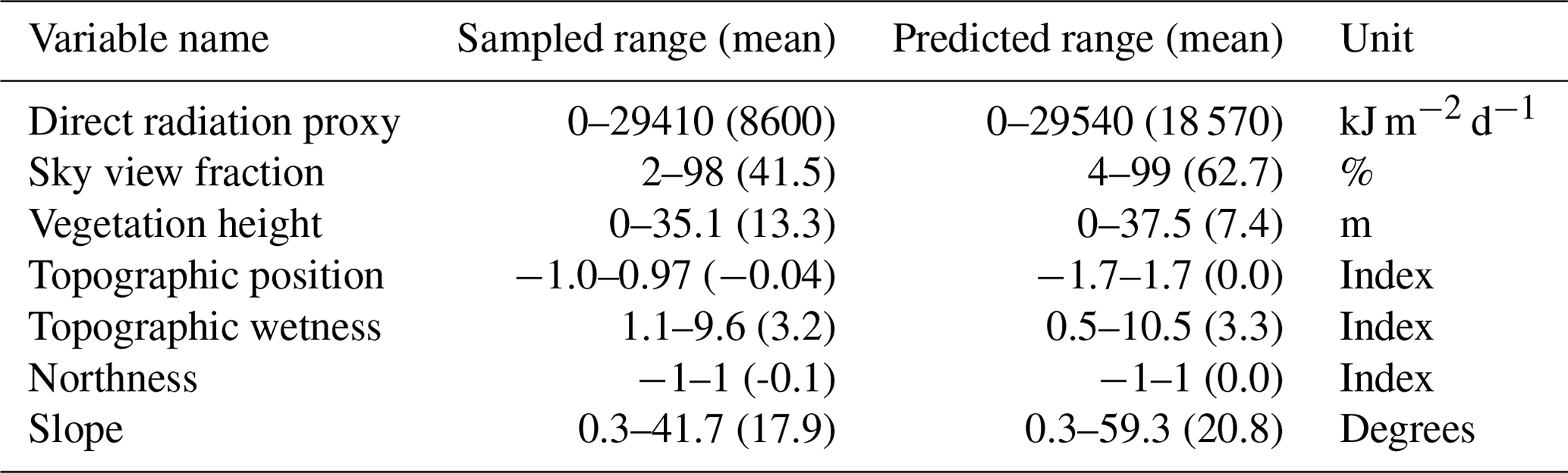
Table C1Descriptive statistics for temperature offsets (∘C). The values indicate the range (and mean between brackets) calculated by deducting the microclimate temperature from the lapse-rate-corrected macroclimate temperature. Negative offset values thus indicate cooler microclimates compared to the macroclimate and vice versa. All means were significantly (p<0.01) different from zero.
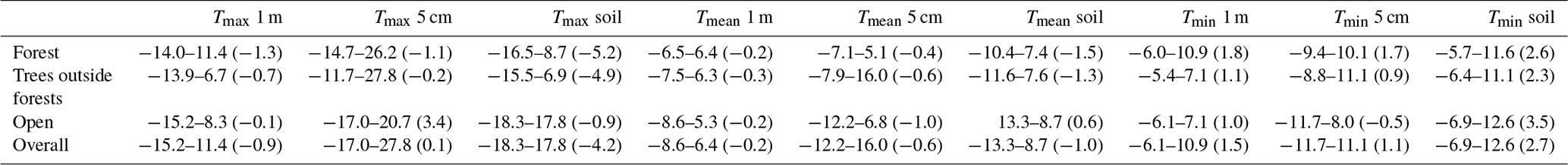
Table D1Predictive performance of microclimate models as quantified using block cross-validation. We also report the predicted offset ranges (minimum to maximum, with mean in brackets), calculated as the difference between the predicted microclimate and the macroclimate.
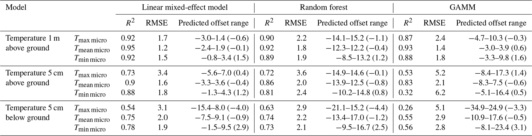
Table E1Comparison of model performance based on block cross-validation of microclimate models against macroclimate benchmark, i.e. a model using macroclimate as the only predictor variable for microclimate. We thus report the performance of the benchmark models (i.e. Macro) alongside the full microclimate models (i.e. Micro) using all predictor variables as explained in the main text. The numbers in brackets show the results based on 5-fold cross-validation. All results are based on linear mixed-effect models.
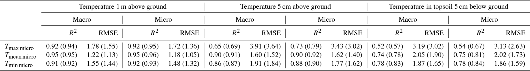
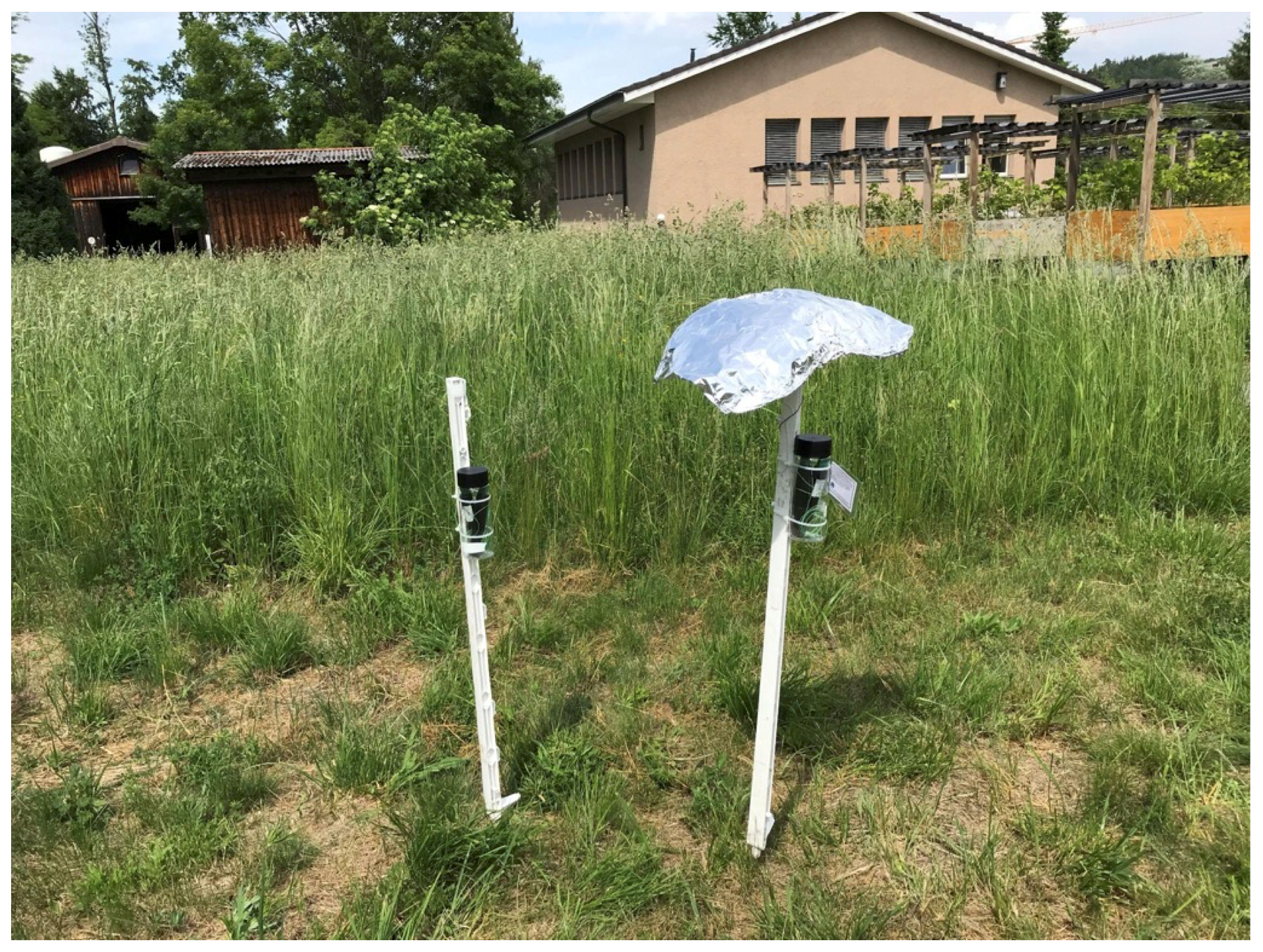
Figure F1Example of shielding experiment with aluminium foil to determine if the logger measurements were affected by direct sunlight on the thermocouple. The thermocouple on the right pole was placed such that it was shaded throughout the day. The actual experiment consisted of a paired design, where we placed two shielded and two unshielded thermocouples in each of three representative environments for the field sampling (open, trees outside forests, and forest).
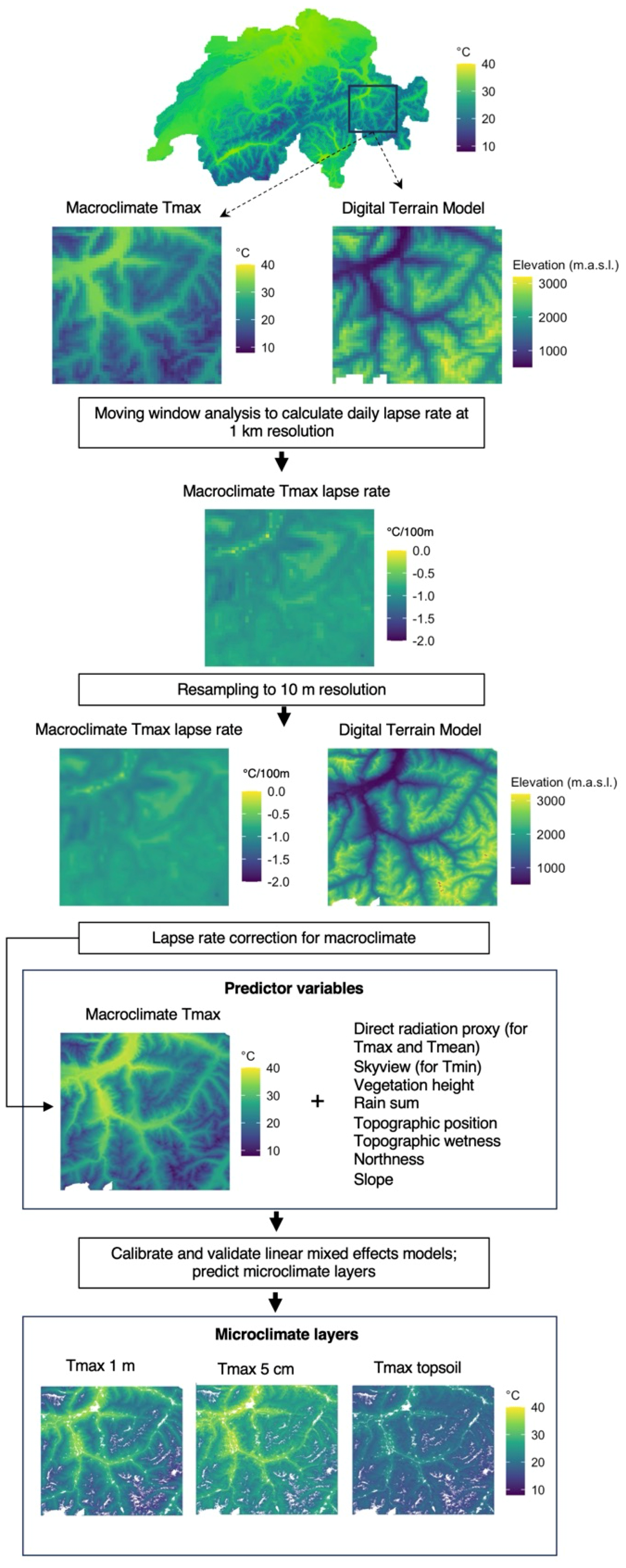
Figure G1Flowchart describing the data processing and modelling pipeline. We used daily macroclimate rasters and a digital terrain model at 1 km resolutions to calculate daily lapse rate maps, which were resampled to 10 m resolution and used to apply a lapse rate correction to our macroclimate layers. Together with other predictor variables we used the lapse-rate-corrected macroclimate layers to predict our microclimate layers at different vertical heights. Please note that, for illustration purposes, all temperature maps show daily maximum temperatures prevailing on 31 July 2018.
The monthly aggregated microclimate maps, as well as the monthly transmissivity maps, will be made publicly available on Envidat, a permanent data repository managed by WSL (Sulmoni et al., 2023). The daily microclimate maps are freely available upon request. The radiation model CanRad is available on https://github.com/c-webster/CanRad.jl (Webster et al., 2023).
FZ designed the study with input from NEZ and PDF. ES, FZ, and DF collected the microclimate data. ES, FZ, JTM, and CW performed the data analyses and modelling, with input from DNK and TJ. AB and CG provided the data. FZ and CW wrote the paper. All the authors provided feedback on the paper.
The contact author has declared that none of the authors has any competing interests.
Publisher's note: Copernicus Publications remains neutral with regard to jurisdictional claims made in the text, published maps, institutional affiliations, or any other geographical representation in this paper. While Copernicus Publications makes every effort to include appropriate place names, the final responsibility lies with the authors.
We are grateful to all the landowners for granting access and supporting us with the field measurements, to the Federal Office of Meteorology and Climatology (MeteoSwiss) for providing macroclimate data, and to the Canton Ticino for support.
This research has been supported by the Schweizerischer Nationalfonds zur Förderung der Wissenschaftlichen Forschung (grant no. 193645).
This paper was edited by Paul Stoy and reviewed by Jonas Lembrechts and one anonymous referee.
Ashcroft, M. B. and Gollan, J. R.: Moisture, thermal inertia, and the spatial distributions of near-surface soil and air temperatures: Understanding factors that promote microrefugia, Agr. Forest Meteorol., 176, 77–89, https://doi.org/10.1016/j.agrformet.2013.03.008, 2013.
Bates, D., Mächler, M., Bolker, B., and Walker, S.: Fitting Linear Mixed-Effects Models Using lme4, J. Stat. Softw., 67, 1–48, https://www.jstatsoft.org/article/view/v067i01 (last access: 19 January 2024), 2015.
Bode, C. A., Limm, M. P., Power, M. E., and Finlay, J. C.: Subcanopy Solar Radiation model: Predicting solar radiation across a heavily vegetated landscape using LiDAR and GIS solar radiation models, Remote Sens. Environ., 154, 387–397, https://doi.org/10.1016/j.rse.2014.01.028, 2014.
Bramer, I., Anderson, B. J., Bennie, J., Bladon, A. J., De Frenne, P., Hemming, D., Hill, R. A., Kearney, M. R., Körner, C., Korstjens, A. H., Lenoir, J., Maclean, I. M. D., Marsh, C. D., Morecroft, M. D., Ohlemüller, R., Slater, H. D., Suggitt, A. J., Zellweger, F., and Gillingham, P. K.: Advances in Monitoring and Modelling Climate at Ecologically Relevant Scales, Adv. Ecol. Res., 58, 101–161, https://doi.org/10.1016/bs.aecr.2017.12.005, 2018.
Brändli, U.-B., Abegg, M., and Allgaier Leuch, B.: Schweizerisches Landesforstinventar, Ergebnisse der vierten Erhebung 2009–2017, Birmensdorf, Eidgenössische Forschungsanstalt für Wald, Schnee und Landschaft WSL, Bern, Bundesamt für Umwelt, 341 pp., https://doi.org/10.16904/envidat.146, 2020.
Chen, J., Saunders, S. C., Crow, T. R., Naiman, R. J., Brosofske, K. D., Mroz, G. D., Brookshire, B. L., and Franklin, J. F.: Microclimate in forest ecosystem and landscape ecology: Variations in local climate can be used to monitor and compare the effects of different management regimes, Bioscience, 49, 288–297, 1999.
Christiansen, D. M., Iversen, L. L., Ehrlén, J., and Hylander, K.: Changes in forest structure drive temperature preferences of boreal understorey plant communities, J. Ecol., 110, 631–643, https://doi.org/10.1111/1365-2745.13825, 2022.
Daly, C., Halbleib, M., Smith, J. I., Gibson, W. P., Doggett, M. K., Taylor, G. H., Curtis, J., and Pasteris, P. P.: Physiographically sensitive mapping of climatological temperature and precipitation across the conterminous United States, Int. J. Climatol., 28, 2031–2064, https://doi.org/10.1002/joc.1688, 2008.
De Frenne, P., Zellweger, F., Rodriìguez-Saìnchez, F., Scheffers, B., Hylander, K., Luoto, M., Vellend, M., Verheyen, K., and Lenoir, J.: Global buffering of temperatures under forest canopies, Nat. Ecol. Evol., 3, 744–749, 2019.
De Frenne, P., Lenoir, J., Luoto, M., Scheffers, B. R., Zellweger, F., Aalto, J., Ashcroft, M. B., Christiansen, D. M., Decocq, G., De Pauw, K., Govaert, S., Greiser, C., Gril, E., Hampe, A., Jucker, T., Klinges, D. H., Koelemeijer, I. A., Lembrechts, J. J., Marrec, R., Meeussen, C., Ogée, J., Tyystjärvi, V., Vangansbeke, P., and Hylander, K.: Forest microclimates and climate change: Importance, drivers and future research agenda, Glob. Change Biol., 27, 2279–2297, https://doi.org/10.1111/gcb.15569, 2021.
Dobrowski, S. Z.: A climatic basis for microrefugia: the influence of terrain on climate, Glob. Change Biol., 17, 1022–1035, https://doi.org/10.1111/j.1365-2486.2010.02263.x, 2011.
Duffy, J. P., Anderson, K., Fawcett, D., Curtis, R. J., and Maclean, I. M. D.: Drones provide spatial and volumetric data to deliver new insights into microclimate modelling, Landsc. Ecol. Eng., 9, 685–702, https://doi.org/10.1007/s10980-020-01180-9, 2021.
FOEN: Federal Office for the Environment: Swiss Forest Ecoregeions https://opendata.swiss/en/dataset/waldstandortsregionen (last access: 15 January 2024), 2022.
Freeman, T. G.: Calculating catchment area with divergent flow based on a regular grid, Comput. Geosci., 17, 413–422, https://doi.org/10.1016/0098-3004(91)90048-I, 1991.
Frei, C.: Interpolation of temperature in a mountainous region using nonlinear profiles and non-Euclidean distances, Int. J. Climatol., 34, 1585–1605, https://doi.org/10.1002/joc.3786, 2014.
Frey, S. J. K., Hadley, A. S., Johnson, S. L., Schulze, M., Jones, J. A., and Betts, M. G.: Spatial models reveal the microclimatic buffering capacity of old-growth forests, Sci. Adv., 2, e1501392, https://doi.org/10.1126/sciadv.1501392, 2016.
Geiger, R., Aron, R. H., and Todhunter, P.: The climate near the ground, Rowman and Littlefield, Oxford, ISBN-10 0742518574, 2009.
Greiser, C., Meineri, E., Luoto, M., Ehrlén, J., and Hylander, K.: Monthly microclimate models in a managed boreal forest landscape, Agr. Forest Meteorol., 250–251, 147–158, https://doi.org/10.1016/j.agrformet.2017.12.252, 2018.
Haesen, S., Lembrechts, J. J., De Frenne, P., Lenoir, J., Aalto, J., Ashcroft, M. B., Kopecký, M., Luoto, M., Maclean, I., Nijs, I., Niittynen, P., van den Hoogen, J., Arriga, N., Brůna, J., Buchmann, N., Čiliak, M., Collalti, A., De Lombaerde, E., Descombes, P., Gharun, M., Goded, I., Govaert, S., Greiser, C., Grelle, A., Gruening, C., Hederová, L., Hylander, K., Kreyling, J., Kruijt, B., Macek, M., Máliš, F., Man, M., Manca, G., Matula, R., Meeussen, C., Merinero, S., Minerbi, S., Montagnani, L., Muffler, L., Ogaya, R., Penuelas, J., Plichta, R., Portillo-Estrada, M., Schmeddes, J., Shekhar, A., Spicher, F., Ujházyová, M., Vangansbeke, P., Weigel, R., Wild, J., Zellweger, F., and Van Meerbeek, K.: ForestClim – Bioclimatic variables for microclimate temperatures of European forests, Glob. Change Biol., 29, 2886–2892, https://doi.org/10.1111/gcb.16678, 2023a.
Haesen, S., Lenoir, J., Gril, E., De Frenne, P., Lembrechts, J. J., Kopecký, M., Macek, M., Man, M., Wild, J., and Van Meerbeek, K.: Microclimate reveals the true thermal niche of forest plant species, Ecol. Lett., 26, 2043–2055, https://doi.org/10.1111/ele.14312, 2023b.
Jones, H. G.: Plants and microclimate, A quantitative approach to environmental plant physiology, 3rd Edn., Cambridge, Cambridge University Press, ISBN: 10 0521279593, 2014.
Jucker, T., Hardwick, S. R., Both, S., Elias, D. M. O., Ewers, R. M., Milodowski, D. T., Swinfield, T., and Coomes, D. A.: Canopy structure and topography jointly constrain the microclimate of human-modified tropical landscapes, Glob. Change Biol., 24, 5243–5258, 2018.
Kearney, M. R. and Porter, W. P.: NicheMapR – an R package for biophysical modelling: the microclimate model, Ecography, 40, 664–674, https://doi.org/10.1111/ecog.02360, 2017.
Kearney, M. R., Gillingham, P. K., Bramer, I., Duffy, J. P., and Maclean, I. M. D.: A method for computing hourly, historical, terrain-corrected microclimate anywhere on earth, Method. Ecol. Evol., 11, 38–43, https://doi.org/10.1111/2041-210X.13330, 2020.
Kükenbrink, D., Schneider, F. D., Schmid, B., Gastellu-Etchegorry, J. P., Schaepman, M. E., and Morsdorf, F.: Modelling of three-dimensional, diurnal light extinction in two contrasting forests, Agr. Forest Meteorol., 296, 108230, https://doi.org/10.1016/j.agrformet.2020.108230, 2021.
Lembrechts, J. J., Lenoir, J., Roth, N., Hattab, T., Milbau, A., Haider, S., Pellissier, L., Pauchard, A., Ratier Backes, A., Dimarco, R. D., Nuñez, M. A., Aalto, J., and Nijs, I.: Comparing temperature data sources for use in species distribution models: From in-situ logging to remote sensing, Glob. Ecol. Biogeogr., 28, 1578–1596, https://doi.org/10.1111/geb.12974, 2019a.
Lembrechts, J. J., Nijs, I., and Lenoir, J.: Incorporating microclimate into species distribution models, Ecography, 42, 1267–1279, https://doi.org/10.1111/ecog.03947, 2019b.
Lembrechts, J. J., Aalto, J., Ashcroft, M. B., et al.: SoilTemp: a global database of near-surface temperature, Glob. Change Biol., 26, 6616–6629, https://doi.org/10.1111/gcb.15123, 2020.
Lembrechts, J. J., van den Hoogen, J., Aalto, J., et al.: Global maps of soil temperature, Glob. Change Biol., 28, 3110–3144, https://doi.org/10.1111/gcb.16060, 2022.
Liaw, A. and Wiener, M.: Classification and Regression by Random forest, R News, 2, 18–22, 2002.
Maclean, I. M. D. and Early, R.: Macroclimate data overestimate range shifts of plants in response to climate change, Nat. Clim. Change, 13, 484–490, https://doi.org/10.1038/s41558-023-01650-3, 2023.
Maclean, I. M. D. and Klinges, D. H.: Microclimc: A mechanistic model of above, below and within-canopy microclimate, Ecol. Modell., 451, 109567, https://doi.org/10.1016/j.ecolmodel.2021.109567, 2021.
Maclean, I. M. D., Mosedale, J. R., and Bennie, J. J.: Microclima: an R package for modelling meso- and microclimate, Method. Ecol. Evol., 10, 280–290, https://doi.org/10.1111/2041-210X.13093, 2018.
Maclean, I. M. D., Duffy, J. P., Haesen, S., Govaert, S., De Frenne, P., Vanneste, T., Lenoir, J., Lembrechts, J. J., Rhodes, M. W., and Van Meerbeek, K.: On the measurement of microclimate, Method. Ecol. Evol., 12, 1397–1410, https://doi.org/10.1111/2041-210X.13627, 2021.
Malkoç, E., Rüetschi, M., Ginzler, C., and Waser, L. T.: Countrywide mapping of trees outside forests based on remote sensing data in Switzerland, Int. J. Appl. Earth Obs. Geoinf., 100, 102336, https://doi.org/10.1016/j.jag.2021.102336, 2021.
Musselman, K. N., Margulis, S. A., and Molotch, N. P.: Estimation of solar direct beam transmittance of conifer canopies from airborne LiDAR, Remote Sens. Environ., 136, 402–415, https://doi.org/10.1016/j.rse.2013.05.021, 2013.
Potter, K. A., Arthur Woods, H., and Pincebourde, S.: Microclimatic challenges in global change biology, Glob. Change Biol., 19, 2932–2939, https://doi.org/10.1111/gcb.12257, 2013.
Roberts, D. R., Bahn, V., Ciuti, S., Boyce, M. S., Elith, J., Guillera-Arroita, G., Hauenstein, S., Lahoz-Monfort, J. J., Schröder, B., Thuiller, W., Warton, D. I., Wintle, B. A., Hartig, F., and Dormann, C. F.: Cross-validation strategies for data with temporal, spatial, hierarchical, or phylogenetic structure, Ecography, 40, 913–929, https://doi.org/10.1111/ecog.02881, 2017.
Scherrer, D. and Körner, C.: Infra-red thermometry of alpine landscapes challenges climatic warming projections, Glob. Change Biol., 16, 2602–2613, https://doi.org/10.1111/j.1365-2486.2009.02122.x, 2010.
Senf, C. and Seidl, R.: Mapping the forest disturbance regimes of Europe, Nat. Sustain., 4, 63–70, https://doi.org/10.1038/s41893-020-00609-y, 2021.
Suggitt, A. J., Wilson, R. J., Isaac, N. J. B., Beale, C. M., Auffret, A. G., August, T., Bennie, J. J., Crick, H. Q. P., Duffield, S., Fox, R., Hopkins, J. J., Macgregor, N. A., Morecroft, M. D., Walker, K. J., and Maclean, I. M. D.: Extinction risk from climate change is reduced by microclimatic buffering, Nat. Clim. Change, 8, 713–717, https://doi.org/10.1038/s41558-018-0231-9, 2018.
Sulmoni, E., De Frenne, P., Zimmermann, N., Frey, D. J., Karger, D., Malle, J., Webster, C., Jonas, T., Ginzler, C., Baltensweiler, A., and Zellweger, F.: Monthly topsoil and near surface microclimate temperature data for Switzerland, EnviDat [data set], https://doi.org/10.16904/envidat.431, 2023.
Swisstopo: Height Models https://www.swisstopo.admin.ch/en/geodata/height.html (last access: 15 January 2024), 2020.
Swisstopo: VECTOR25, https://www.swisstopo.admin.ch/de/geodata/maps/smv/smv25.html (last access: 15 January 2024), 2022.
Tymen, B., Vincent, G., Courtois, E. A., Heurtebize, J., Dauzat, J., Marechaux, I., and Chave, J.: Quantifying micro-environmental variation in tropical rainforest understory at landscape scale by combining airborne LiDAR scanning and a sensor network, Ann. Forest Sci., 74, 32, https://doi.org/10.1007/s13595-017-0628-z, 2017.
Vanneste, T., Govaert, S., Spicher, F., Brunet, J., Cousins, S. A. O., Decocq, G., Diekmann, M., Graae, B. J., Hedwall, P. O., Kapás, R. E., Lenoir, J., Liira, J., Lindmo, S., Litza, K., Naaf, T., Orczewska, A., Plue, J., Wulf, M., Verheyen, K., and De Frenne, P.: Contrasting microclimates among hedgerows and woodlands across temperate Europe, Agr. Forest Meteorol., 281, 107818, https://doi.org/10.1016/j.agrformet.2019.107818, 2020.
von Arx, G., Graf Pannatier, E., Thimonier, A., Rebetez, M., and Gilliam, F.: Microclimate in forests with varying leaf area index and soil moisture: potential implications for seedling establishment in a changing climate, J. Ecol., 101, 1201–1213, https://doi.org/10.1111/1365-2745.12121, 2013.
Waser, L. T., Ginzler, C., and Rehush, N.: Wall-to-Wall tree type mapping from countrywide airborne remote sensing surveys, Remote Sens., 9, 1–24, https://doi.org/10.3390/rs9080766, 2017.
Webster, C., Rutter, N., Zahner, F., and Jonas, T.: Modeling subcanopy incoming longwave radiation to seasonal snow using air and tree trunk temperatures, J. Geophys. Res.-Atmos., 121, 1220–1235, https://doi.org/https://doi.org/10.1002/2015JD024099, 2016.
Webster, C., Mazzotti, G., Essery, R., and Jonas, T.: Enhancing airborne LiDAR data for improved forest structure representation in shortwave transmission models, Remote Sens. Environ., 249, 112017, https://doi.org/10.1016/j.rse.2020.112017, 2020.
Webster, C., Essery, R., Mazzotti, G., and Jonas, T.: Using just a canopy height model to obtain lidar-level accuracy in 3D forest canopy shortwave transmissivity estimates, Agr. Forest Meteorol., 338, 109429, https://doi.org/10.1016/j.agrformet.2023.109429, 2023 (model code available at https://github.com/c-webster/CanRad.jl, last access: 19 January 2024).
Wood, S. N.: Generalized Additive Models: An Introduction with R, 2nd Edn., Chapman and Hall/CRC, https://doi.org/10.1201/97813153702792017, 2017.
Zellweger, F., Frenne, P. De, Lenoir, J., Rocchini, D., and Coomes, D.: Advances in microclimate ecology arising from remote sensing, Trends Ecol. Evol., 34, 327–341, https://doi.org/10.1016/j.tree.2018.12.012, 2019a.
Zellweger, F., Baltensweiler, A., Schleppi, P., Huber, M., Küchler, M., Ginzler, C., and Tobias, J.: Estimating below-canopy light regimes using airborne laser scanning: an application to plant community analysis, Ecol. Evol., 9, 9149–9159, https://doi.org/10.1002/ece3.5462, 2019b.
Zellweger, F., Coomes, D., Lenoir, J., Depauw, L., Maes, S. L., Wulf, M., Kirby, K., Brunet, J., Kopecky, M., Malis, F., Schmidt, W., Heinrichs, S., Ouden, J. den, Jaroszewicz, B., Buyse, G., Spicher, F., Verheyen, K., and De Frenne, P.: Seasonal drivers of understorey temperature buffering in temperate deciduous forests across Europe, Glob. Ecol. Biogeogr., 28, 1774–1786, 2019c.
Zellweger, F., De Frenne, P., Lenoir, J., Vangansbeke, P., Verheyen, K., Bernhardt-Römermann, M., Baeten, L., Hédl, R., Berki, I., Brunet, J., Van Calster, H., Chudomelová, M., Decocq, G., Dirnböck, T., Durak, T., Heinken, T., Jaroszewicz, B., Kopecký, M., Máliš, F., Macek, M., Malicki, M., Naaf, T., Nagel, T. A., Ortmann-Ajkai, A., Petřík, P., Pielech, R., Reczyńska, K., Schmidt, W., Standovár, T., Świerkosz, K., Teleki, B., Vild, O., Wulf, M., and Coomes, D.: Forest microclimate dynamics drive plant responses to warming, Science, 368, 772–775, https://doi.org/10.1126/science.aba6880, 2020.
Zimmermann, N. E. and Roberts, D. W.: Final report of the MLP climate and biophysical mapping project, Swiss Federal Research Inst. WSL, Birmensdorf, Switzerland and Utah State Univ., Logan, USA, 2001.
- Abstract
- Introduction
- Materials and methods
- Results
- Discussion
- Appendix A: Logger sensitivity analysis
- Appendix B
- Appendix C
- Appendix D
- Appendix E
- Appendix F
- Appendix G
- Code and data availability
- Author contributions
- Competing interests
- Disclaimer
- Acknowledgements
- Financial support
- Review statement
- References