Investigating ecosystem connections in the shelf sea environment using complex networks

We use complex network theory to better represent and understand the ecosystem connectivity in a shelf sea environment. The baseline data used for the analysis are obtained from a state-of-the-art coupled marine physics–biogeochemistry model simulating the North West European Shelf (NWES). The complex network built on model outputs is used to identify the functional groups of variables behind the biogeochemistry dynamics, suggesting how to simplify our understanding of the complex web of interactions within the shelf sea ecosystem. We demonstrate that complex networks can also be used to understand spatial ecosystem connectivity, identifying both the (geographically varying) connectivity length-scales and the clusters of spatial locations that are connected. We show that the biogeochemical length-scales vary significantly between variables and are not directly transferable. We also find that the spatial pattern of length-scales is similar across each variable, as long as a specific scaling factor for each variable is taken into account. The clusters indicate geographical regions within which there is a large exchange of information within the ecosystem, while information exchange across the boundaries between these regions is limited. The results of this study describe how information is expected to propagate through the shelf sea ecosystem, and how it can be used in multiple future applications such as stochastic noise modelling, data assimilation, or machine learning.

1 Introduction

Although shelf seas, understood as the seas covering parts of a continental shelf, are only 7 % of the global ocean, they are responsible for 20 % of the global biological productivity, contribute to 20 % of the ocean uptake of atmospheric carbon, and are the grounds for 80 % of global fish catches (Pauly et al., 2002; Borges et al., 2006; Jahnke, 2010; Legge et al., 2020). For the European economy, the North West European Shelf (NWES) is of key importance. Numerical models such as the European Regional Seas Ecosystem Model (ERSEM) have been developed in an effort to understand and predict marine ecosystem behaviour and the cycling of chemical elements such as carbon, nitrogen, or phosphorus (Heinze and Gehlen, 2013; Butenschön et al., 2016; Ford et al., 2018). However, marine biogeochemistry is complex to simulate, e.g. the ERSEM model contains more than 50 pelagic variables and hundreds of parameters (Butenschön et al., 2016), representing a plethora of processes. Such a complex model is computationally costly, which often makes it too expensive to address certain questions that require large ensemble simulations, such as those addressing an ecosystem's response to climate change and anthropogenic pressures across a large variety of scenarios, or to explore what-if types of analyses for management and policy-making scenarios. Nevertheless, it may be possible to gain insights into such questions through statistical tools, leading to innovative representations of complex model outputs, such as those based on network theory (Zanin et al., 2016; Albert and Barabási, 2002), and using them to construct reduced complexity models, such as (but not exclusively) machine learning (ML) emulators (Schartau et al., 2017; Sonnewald et al., 2021).

Networks are a mathematical tool for modelling the key relationships/connections between objects/data. Typically, most networks generated from real-world data are complex networks with examples being found in biochemical systems, neural networks, social networks, the Internet, and the World Wide Web (Boccaletti et al., 2006). Within the context of environmental networks, particularly for highly multivariate cases such as biogeochemical marine ecology, networks offer an intuitive human-interpretable view of the highly interconnected spatio-temporal regions and variables (Tsonis et al., 2006) that can often be critical to the resilience of a given system (Barabási and Bonabeau, 2003; Jeong et al., 2001), as well as to better understand how certain pressures or changes in the environment will propagate across the system (Jiang et al., 2018). By using complex networks, we gain insight into the structure of the data and the patterns that form but also information that will allow for smarter decision-making when considering data sampling and feature selection for ML.

In this work, we use complex networks (CNs) and associated statistical analyses, together with NWES as a test case, to investigate three relevant topics related to shelf sea biogeochemistry. (i) We used the network connectivity to estimate the spatial horizontal correlation length-scales of the biogeochemical variables. Typically, spatial-correlation functions are identified either through ensemble runs or diagnostic methods (Hollingsworth and Lönnberg, 1986; Desroziers et al., 2005). Horizontal correlation length-scale analysis provides important parameter fits for the horizontal correlation functions that can be used in the operational marine forecasting systems, e.g. applying variational data assimilation (DA), using parameterized background covariances. Furthermore, such length-scales can also inform localization factors within an ensemble DA method. Both have applications in the UK operational system for the NWES, run at the UK Met Office, whether in its variational version (e.g. Edwards et al., 2012; Waters et al., 2015; Skákala et al., 2018; Fowler et al., 2023) or in the newly developed ensemble-variational version (e.g. Lea et al., 2022). Since future observational missions will provide new biogeochemical variables (such as nutrients or pH) for assimilation (Skákala et al., 2021; Ford, 2021), it is of crucial importance to gain understanding of how transferable the horizontal correlation length-scales are between the different biogeochemical variables. (ii) We exploited network clustering algorithms to demonstrate how a shelf sea can be split into geographic regions, based on high ecosystem inter-connectivity within the regional boundaries and a little beyond them. Because of the significant connectivity in the ecosystem within each identified region, we do expect that ecosystem characteristics will remain similar within the regional boundaries, thus justifying a region-informed modelling strategy. (iii) Finally, we used CNs to identify the local interactions between the modelled biogeochemical variables, subsequently grouping these variables into sets of functional groups (i.e. a set of state variables that are highly correlated with each other). These are also important to select and guide new observational missions.

The analysis from this study can provide additional information to biogeochemistry modellers for building simplified (yet realistic with respect to the objectives) and computationally cheaper models than ERSEM, capable of simulating a wide range of what-if scenarios. Simultaneously, it can identify the necessary model complexity to realistically simulate the NWES biogeochemistry. Finally, for the goal of developing efficient ML-based emulators for ERSEM or for some of its critical parameterizations or sub-components, this study paves the way for how to perform efficient feature selection (i.e. how to select the minimum number of input variables to achieve the desired accuracy).

The paper is organized as follows. We first give, in Sect. 2, details on the model used, explaining each component used to output the data we analysed, as well as the relevant configurations for each component. In Sect. 3 we discuss the methods used, starting with the pre-processing step used to remove the seasonal signal from the data analysed. We then detail the approach used to estimate the mean length-scale of each biogeochemical variable, as well as how we develop a series of spatial networks that help to efficiently capture the spatial variability of these length-scales. We then explain the clustering algorithm used on these networks that splits the shelf sea into a set of regions. The final part of the methodology moves away from the spatial analysis of the variables and gives details on how we developed a CN to compare the inter-variable interactions and clusters that form. Following this, we present and discuss our results in Sect. 4, with each subsection corresponding to a subsection of the methodology. We finish with concluding remarks, in Sect. 5, summarizing the key findings and discussing future work.

Table 1 The ERSEM pelagic variables.

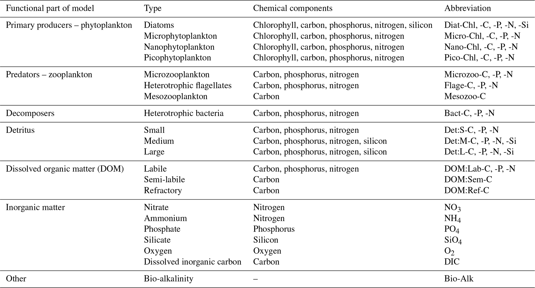
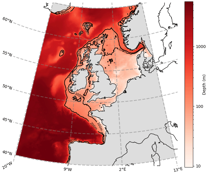
Figure 1 The Atlantic Margin Model (AMM7) domain used in this study. The figure also shows the ocean bathymetry of the North West European Shelf.

2 Model and data

To obtain a complex picture of the shelf sea biogeochemistry, including the relationships between the variety of key biogeochemical variables (detailed in Table 1), the observations are far from sufficient, as any robust observations are limited to only very specific variables, i.e. total or phytoplankton functional type (PFT) surface chlorophyll obtained from the satellite ocean colour (Groom et al., 2019). Even those robust observations, exclusively obtained from the satellite, have many data gaps and spatially correlated errors that make their use unsuitable for this type of analysis. Any other observations are typically very rare and extremely sparse (Telszewski et al., 2018) and so provide almost no information on the connectivity between variables and spatial locations across the shelf sea domain. To overcome this limitation to analyse the shelf sea ecosystem connectivity, we used the complex network theory to study the daily NWES surface outputs of a 3-year-long (2016–2018) run of the coupled hydrodynamic-biogeochemical ecosystem model NEMO–FABM–ERSEM.¹ The outputs were obtained from a configuration at 7 km grid size, on the Atlantic Margin Model (AMM7) domain (see Fig. 1). Reducing the dataset to only surface outputs will have some limitations (e.g. the relationship between detritus and phytoplankton and zooplankton may not be fully captured due to sinking particles); however, we believe that using surface data is still the most useful way to make the analysis affordable, as (i) it will capture the connections in the mixed layer, which is the most biologically active part of the ocean, and (ii) it is directly relevant to DA horizontal length-scales near the surface, which is where most of the NWES observations are located. The analysis was also repeated on a subset of variables for an independent 3-year-long period between 2005–2007 with a similar outcome (not shown). The physics and biogeochemistry components of the coupled model that produced those simulations are described below.

2.1 Physical model: NEMO

The NEMO ocean physics component (OPA) is a finite-difference, hydrostatic, primitive equation ocean general circulation model (Madec, 2015). The specific NEMO configuration used in this study has been described in Skákala et al. (2020): it is known as CO6 NEMO and is based on NEMOv3.6, which is a development of the CO5 configuration described by O'Dea et al. (2017). For details on the NEMOv3.6 setup, such as the generic length-scale turbulence scheme used to calculate the turbulent viscosities and diffusivities, see O'Dea et al. (2017). The model has a spatial resolution of 7 km on the AMM7 domain and employs a terrain-following $z^{\ast }-\mathit{\sigma }$ coordinate system with 51 vertical levels (Siddorn and Furner, 2013). The lateral boundary conditions for physical variables at the Atlantic boundary were obtained from the outputs of the UK Met Office's $\mathrm{1}/\mathrm{12}$^∘ North Atlantic model (NATL12) (Storkey et al., 2010), while the Baltic boundary values were derived from a reanalysis produced by the Danish Meteorological Institute for Copernicus Marine Environment Monitoring Service (CMEMS). The model was forced at the surface using atmospheric fluxes from an hourly and 31 km resolution realization (HRES) of the ERA5 dataset (https://www.ecmwf.int/, last access: 1 March 2023).

2.2 Biogeochemical model: ERSEM

ERSEM (Baretta et al., 1995; Butenschön et al., 2016) is a marine biogeochemistry model that simulates lower trophic levels of the ocean ecosystem, including plankton and benthic fauna (Blackford, 1997). The ERSEM 50 pelagic state variables are listed in Table 1. The model divides phytoplankton into four functional types based on size: picophytoplankton, nanophytoplankton, microphytoplankton, and diatoms (Baretta et al., 1995). ERSEM uses variable stoichiometry for the simulated plankton groups (Baretta-Bekker et al., 1997; Geider et al., 1997) and represents the biomass of each functional type in terms of chlorophyll, carbon, nitrogen, and phosphorus, with diatoms also being represented by silicon. ERSEM predators consist of three types of zooplankton (mesozooplankton, microzooplankton, and heterotrophic nanoflagellates), with organic material being decomposed by a single type of heterotrophic bacteria (Butenschön et al., 2016). The model represents three different types of detritus and three types of dissolved organic matter (DOM). The inorganic component of ERSEM includes nutrients such as nitrate, phosphate, silicate, ammonium, and carbon, as well as dissolved oxygen. The carbonate system is also included in the model (Artioli et al., 2012).

Both the physical and biogeochemical models were forced by daily-varying river discharge data from Lenhart et al. (2010) and initialized from the CMEMS reanalysis produced at the Met Office (product CMEMS-NWS-QUID-004-011; https://marine.copernicus.eu/services-portfolio/access-to-products/, last access: 1 March 2023).

3 Methodology

3.1 Data pre-processing

In order to extract non-trivial interactions and dynamics of the system, we removed the dominating seasonal signal. Typically, this is achieved by phase-averaging and standardizing the data to generate an anomaly time series (with respect to climatology) with zero mean and unit variance. However, with our high temporal resolution (daily) but just 3 years of data, this phase-averaging method can heavily skew a dataset with both high inter-annual and daily variability. As a result, we instead opted to use a high-pass filter that standardizes every time step of data according to its local temporal behaviour (a running average with a 10 d time window), with details given in the following.

First, for each day, we computed the local mean that bears the signature of the seasonality. This is done by averaging the values within a chosen time window centred on that day:

$$\begin{array}{}\text{(1)}& {\mathit{\mu }}_d={\displaystyle \frac{\mathrm{1}}{T}}\sum _{t=-T/\mathrm{2}}^{T/\mathrm{2}}{a}_{d+t},\end{array}$$

where T+1 is the number of days in the window, with T being an even natural number, and a_d+t represents the value in the time series at day d+t, with offset (in days) t. The aim is to remove the seasonal cycle by subtracting μ_d, i.e. a_d−μ_d. Selecting an appropriate window size is crucial in generating a time series with useful properties. For our purpose of removing the seasonal cycle, a relatively short window is appropriate. Following a sensitivity analysis (not shown), we found that a window of T = 10 d efficiently removes the seasonal effect while retaining a functional signal for further analysis. We then take the standard deviation of those same points within the window:

$$\begin{array}{}\text{(2)}& {\mathit{\sigma }}_d=\sqrt{{\displaystyle \frac{\mathrm{1}}{T-\mathrm{1}}}\sum _{t=-T/\mathrm{2}}^{T/\mathrm{2}}(a_{d+t}-{\mathit{\mu }}_d{)}^{\mathrm{2}}}.\end{array}$$

Using the output from both Eqs. (1) and (2), we transform the raw data points into a time-local standardized form:

$$\begin{array}{}\text{(3)}& a_d^{\mathrm{n}}={\displaystyle \frac{a_d-{\mathit{\mu }}_d}{{\mathit{\sigma }}_d}}.\end{array}$$

The data consist of 50 ERSEM state variables (as well as temperature and salinity) on a 375 × 297 horizontal grid using only the surface layer with 1094 d (> 6 billion data points). Following the pre-processing stage, the data will have a mean of 0 and unit variance relative to each point's surrounding temporal behaviour, as set by the window size of 10. The primary purpose of this procedure is to filter out the seasonality (example given in Fig. S2 in the Supplement) that could dominate any correlation analysis. The procedure also automatically filters out longer time variability (e.g. inter-annual), but such variability cannot be properly represented by the 3-year data anyway. Despite the short timescales used in the analysis, we do expect that the dominant interactions on these timescales would likely remain to be the dominant factor in any (non-filtered) long-term connectivity analyses. However, a certain level of caution might be still healthy if these results were used for climate-focused what-if scenarios. All data used in this study have been pre-processed using the procedure in Eqs. (1)–(3).

As hinted to above, our method is designed to mitigate (or possibly remove) the skewness caused by instances of high inter-annual variability (those would eventually not be an issue when working with a dataset on a much longer period than 3 years). Furthermore, the proposed approach is still effective in removing the seasonal cycle from data, and it is more sensitive than phase-averaging to dynamics in both low- and high-activity periods of the time series. A key limitation is that the method is not suitable if we had intended to compare data points and times that are separated by an offset significantly larger than T.

3.2 Horizontal correlation length-scale estimates

3.2.1 Biogeochemical length-scale estimation

To estimate the horizontal length-scale of each biogeochemical variable, we calculated a Spearman's correlation between the time series at a reference point and all of its surrounding points simultaneously, within a selected radius. This should reduce the number of unnecessary computations while still being confidently large enough to capture the length-scales. We intentionally chose to use the Spearman correlation in order to capture the non-linear relation that would have been otherwise masked with the Pearson correlation. Starting with a circle of small radius (7 km in this case), we calculated the mean correlation of grid points within the circle. If this correlation was above some threshold, we increased the radius of the circle and recalculated the new mean. Once the mean correlation dropped below a given threshold, we stopped increasing the radius and took this to be an estimate of the horizontal length-scale at the given threshold. The exact distance calculated for these length-scales changes according to the selected correlation threshold (increasing as the selected threshold decreases). A selection of appropriate thresholds (0.5, 0.6, and 0.7) were chosen to capture the horizontal length-scales that demonstrate a “strong” correlation. While this approach is relatively simple, it provides a quantitative measure of the length-scale, and it can easily be applied to each variable in the system. This does assume the ocean is homogeneous and isotropic; while not necessarily true, it is a useful simplification.

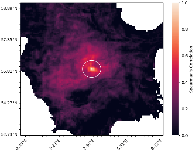
Figure 2 Horizontal length-scale estimate; ℓ = 45.5 km is shown as a white circle, calculated for Diat-Chl with correlation threshold set at 0.5, for a reference point with coordinates 56.10^∘ N, 3.20^∘ E. The colours represent the simultaneous Spearman correlation of each grid point with the central grid point (which is of value 1, as it perfectly correlates with itself).

Figure 2 provides an example for calculating the horizontal length-scale of diatoms chlorophyll (Diat-Chl) with a correlation threshold of 0.5 in the centre of the North Sea.

We averaged these length-scales over 300 sample points for each variable, at least 21 km away from the boundaries, and they were tested at multiple correlation thresholds (0.5, 0.6 and 0.7). These length-scales are used later in Sect. 4.1.

3.2.2 Generating spatial networks

The method used to construct spatial networks from the biogeochemical model is largely inspired by similar applications to models of the climate system (Tsonis et al., 2006). We considered each grid point to be a node in a network for a given variable. In order to generate the links between these nodes, we calculated a Spearman's correlation coefficient between the time series of every pair of nodes for the same variable. To make these comparisons computationally feasible, the grid points are upscaled using arithmetic averaging to a 21 km spatial resolution. To account for the boundaries, we consider a 21 km grid point to be ocean only if more than 50 % of the averaged 7 km points are also ocean.

3.2.3 Estimating horizontal length-scale from the spatial networks

As opposed to the biogeochemical length-scales computed in Sect. 3.2.1, which refer to each variable and reflect their physical properties averaged on the domain, here we introduce a method that enables us to manipulate the spatial networks to look at the structure and spatial dependency of these length-scales. Deducing the length-scales from the networks allows us to bypass the high computational cost associated with the method based on calculating spatial correlations along circles with increasing radii, described in Sect. 3.2.1. The network-based analysis from this section also provides a convenient way to normalize the structure of the spatial patterns found in each variable, without the need to select a specific correlation threshold as in Sect. 3.2.1.

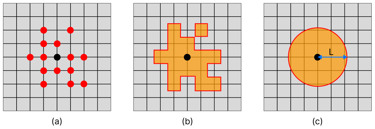
Figure 3 Method for calculating the length-scale of a given node in a network representing the horizontal connectivity of a variable. Panel (a) shows the target node (black) and each of the nodes on the grid that it is linked with (red). Panel (b) shows the area represented by each of the nodes linked to the current target node. Panel (c) shows a circle with equivalent area to the area covered in (b), and the radius L provides us with our approximation of the length-scale at this point.

The approach introduced here started by creating a spatial network for each variable, as described in Sect. 3.2.2. We then pruned each network by removing the links with the weakest correlation, which considers a pair of nodes to be connected only if the correlation coefficient is above a given threshold. The correlation coefficient thresholds used to prune the network of each variable were determined individually, such that each network would contain the same number of links (i.e. the same network density) – effectively normalizing the relational information of each network. This meant that the only differences between the network of any given variable to another were found in the structure of the links. As such, any length-scales calculated for the same geographical point (but different variables) can be directly compared to each other. We calculated a unique length-scale at every 21 km point, for each variable. Figure 3 shows the method used to calculate the length-scale estimation for a given node in a single network (shown as a black dot in the centre of each panel). Figure 3a shows a set of nodes (red) connected to the current target node (black), indicating the surrounding grid points that correlate strongly through time with the current target node. Figure 3b highlights the area represented by this connected set of nodes. Note that the shape of this area is often irregular, but we can generally expect that nodes closer to the target node have a higher chance of being connected. Figure 3c shows a circle with equivalent area to the area highlighted in Fig. 3b. The radius of this circle is used as an approximation of the horizontal length-scale for this node. We assume isotropy and that strong connectivity exists only within this radius, as implied by the transition between Fig. 3a and c. This approximation is a reasonable assumption for the purpose of our analysis as it allows us to make direct comparisons between nodes and across variables, capturing clear and scale-relevant features of the domain. However, it should be noted that these correlations are inherently anisotropic, as we shall see in the regionalization results in Sect. 4.3.

With the spatial variation captured for each variable, we sought to find any underlying structure that was shared between variables across the surface layer. Each of the spatial networks, i.e. N(x,v) where x and v refer to spatial location and variable, respectively, were normalized such that each network contained the same number of links. We then took the mean length-scale at each grid point by averaging the number of connections at each point across all ERSEM state variables, i.e. $M\left(x\right)=\langle N(x,v){\rangle }_v$. To quantify the representativeness of this average, we used Pearson's spatial correlation (PCC) between the spatial distributions of the horizontal length-scales for each variable. Here, if the correlation of $\mathrm{PCC}\left(N\right(x,v),M(x\left)\right)$ for all variables, v, is sufficiently high, then M(x) is representative of N(x,v). Finally, the horizontal length-scale spatial distribution was rescaled to $f\left(x\right)=M\left(x\right)/\langle M\left(x\right){\rangle }_x$, to be more useful in conjunction with the mean length-scales for each variable, found as described in Sect. 3.2.1 and shown in Fig. 4.

3.3 Regionalization using spectral graph clustering

With the spatial networks, the graphs, from Sect. 3.2 at hand, we aimed to cluster geographical points (represented as nodes in each network) so that areas with strongly correlated temporal behaviour are grouped together in a way that is consistent across the set of ERSEM state variables. We used spectral graph clustering (SGC), whereby the spectral properties of key network matrices are considered instead of working on the data directly. In particular, with SGC we partitioned the network into clusters by utilizing the eigenvectors of the Laplacian matrix. This makes it possible to apply the clustering algorithm to “global objects” (the eigenvectors) of the full dataset under study, as opposed to standard applications of clustering methods to the individual entries of the dataset.

For a network with n nodes, the graph Laplacian matrix is a square matrix $\mathbf{L}\in {\mathbb{R}}^{n\times n}$, which can be intended as a discrete (for network) counterpart of the classical Laplacian operator for continuous variables, measuring in this case how the strength of a node changes in its surroundings. For finite dimensional networks, such as those constructed in this work, L is obtained as the difference between the degree matrix, $\mathbf{D}\in {\mathbb{R}}^{n\times n}$, and the weighted adjacency matrix, $\mathbf{W}\in {\mathbb{R}}^{n\times n}$, of the network:

$$\begin{array}{}\text{(4)}& \mathbf{L}=\mathbf{D}-\mathbf{W}.\end{array}$$

Here, W represents the weight of a link between nodes (as defined in this case by the Spearman's correlation between each node on the 21 km grid), and D is a diagonal matrix that represents the sum of the weights that each node has to other nodes. A node with a large degree results in a large diagonal entry in the Laplacian matrix, which may dominate the properties of the matrix. To address this, the Laplacian matrix is normalized to make the influence of these nodes more similar to other lesser-connected nodes, giving

$$\begin{array}{}\text{(5)}& {\mathbf{L}}_{\text{sym}}:={\mathbf{D}}^{-\mathrm{1}/\mathrm{2}}{\mathbf{LD}}^{-\mathrm{1}/\mathrm{2}}=\mathbf{I}-{\mathbf{D}}^{-\mathrm{1}/\mathrm{2}}{\mathbf{WD}}^{-\mathrm{1}/\mathrm{2}}.\end{array}$$

Thanks to this normalization, we can apply a static threshold to each of the networks (as mentioned in Sect. 3.2.2). Once the desired number of clusters, k, is chosen, we compute the first k eigenvectors ${\mathit{u}}_{\mathrm{1}},\mathrm{\dots },{\mathit{u}}_k$ of L_sym and arrange them as columns of matrix $\mathbf{U}\in {\mathbb{R}}^{n\times k}$. We then form the matrix $\mathbf{T}\in {\mathbb{R}}^{n\times k}$ by normalizing the rows of U such that

$$\begin{array}{}\text{(6)}& t_{i,j}=u_{i,j}/{\left(\sum _k{u}_{ik}^{\mathrm{2}}\right)}^{\mathrm{1}/\mathrm{2}}.\end{array}$$

For $i=\mathrm{1},\mathrm{\dots },n$, let y_i∈ℝ^k be a vector corresponding to the ith row of T. Using k-means clustering, we collect the vectors $({\mathit{y}}_i{)}_{i=\mathrm{1},\mathrm{\dots },n}$ into clusters $C_{\mathrm{1}},\mathrm{\dots },C_k$. Finally, we output clusters $A_{\mathrm{1}},\mathrm{\dots },A_k$ with

$$\begin{array}{}\text{(7)}& A_i=\mathit{\left\{}j\right|{\mathit{y}}_j\in C_i\mathit{\}},\end{array}$$

mapping back from the eigenspace and providing a cluster label for each node in the network (Ng et al., 2001; Von Luxburg, 2007).

The method has several characteristics that make it preferable to other clustering methods that are applied to the dataset directly (i.e. k-means clustering, hierarchical clustering, DBSCAN (density-based spatial clustering of applications with noise)). The key advantages of SGC that made it ideal for our purposes are the following. (i) The first is handling non-linearly separable data. Since the eigenvectors of the graph Laplacian capture the structure of the network, they can provide a useful representation of the data even if it is not linearly separable. (ii) The second is being strongly robust to noise. Since the eigenvectors are computed using the entire network, they are less sensitive to noise and outliers compared to traditional clustering methods that rely on individual data points. (iii) The third is identifying clusters of different shapes and sizes. Traditional clustering methods such as k means are limited to identifying spherical clusters of similar size.

Nevertheless, a key challenge in SGC is selecting the appropriate number of clusters to use with the algorithm. A common solution to this problem is to use the “eigengap heuristic” (Tibshirani et al., 2001), which uses the amplitudes and rate of change of the eigenvalues of L_sym to identify the optimal number of clusters. The method suggests that if the difference between the kth and k+1th eigenvalues (an eigengap) is substantial, k is more likely to produce a correct number of clusters. However, if the gap is small, it may lead to less reliable clustering results as perturbations may cause the eigenvectors to be swapped. Our preliminary analysis (not shown) overall indicated no obvious choice for the cluster number, with no significant eigengaps. To address this, we opted to apply the clustering algorithm with every cluster number $\mathrm{1}\le k\le \mathrm{20}$ (an upper bound selected for computational affordability). This allowed us to evaluate the quality of the clusters at different cluster numbers, identifying the values that produce the clearest patterns and structures.

We identified “robust regions” as connected areas of ocean that rarely, or never, contain the boundaries from the clustering of any individual state variable. For the spatial network of each variable, we identified every node that is geographically adjacent to another node with a different cluster label (as found from Eq. 7). These nodes represent the boundaries between different regions. Since each node in a spatial network will have a corresponding node in the spatial network of every other variable (i.e. they share the same geographical point), we could then calculate the frequency with which each geographical point occupies a boundary node, across all ERSEM state variables. These “boundary frequency” values are then plotted onto a grid, according to their geographic location, so that the robust regions can be identified visually.

3.4 Inter-variable interaction networks

The work in the previous sections focused on understanding how each variable separately behaves in horizontal space. In this section, we focused on developing an understanding of how the variables interact with each other co-spatially. This was achieved by assessing the interactions between the different biogeochemical state variables of ERSEM, computing the absolute value of Spearman's rank correlation coefficient between the time series of each variable at an ERSEM grid point. As with before, we chose Spearman's correlation to capture any potential non-linear, monotonic links between variables. These correlations can be represented as a weighted adjacency matrix, where the rows and columns represent each of the variables, and each matrix's entries represents the strength of a pairwise connection between variables at a grid point. As one might expect, the strength of these correlation coefficients will vary spatially. Therefore, in order to identify the most consistent and robust connections (and in a computationally efficient way), we calculated an adjacency matrix for 300 points randomly sampled across the shelf (bathymetry ≤ 200 m) (Borges et al., 2006; Huthnance et al., 2009; Skákala et al., 2022). These 300 matrices are then averaged so that each entry represents the mean of each pairwise comparison. To ensure that these averaged values are reliable, we then calculated the coefficient of variation,

$$\begin{array}{}\text{(8)}& {\mathrm{CV}}_{i,j}={\displaystyle \frac{{\mathit{\sigma }}_{i,j}}{{\mathit{\mu }}_{i,j}}},\end{array}$$

where μ_i,j is the mean of the correlation coefficients (across all 300 sample points) between the time series of variables i and j, and σ_i,j is the standard deviation of the same set of coefficients. This coefficient is then given as a percentage so that we can intuitively view the standard deviation of the correlations as a percentage of the mean.

We accounted for any processes that occur on a lagged or delayed timescale through cross-correlation – determining the degree to which one time series is correlated with another time series after shifting the latter series forward or backward in time. The correlation between any variable pair in the results is always shifted by an offset that maximizes the correlation between the two variables. It should be noted however that, as a result of the pre-processing step applied to the data (cf. Sect. 3.1), the time offset is bound to T; by construction (after the pre-processing), points in a time series that are outside of that range are insensitive to each other.

As this inter-variable analysis provided us with a weighted adjacency matrix, we were once again able to apply the SGC algorithm described in Sect. 3.3. In this instance, the resulting clusters can be interpreted as functional groups of similarly behaving variables, rather than spatial regions of similar behaviour.

4 Results and discussion

4.1 Horizontal spatial correlation length-scale estimates

Figure 4 shows the estimated horizontal correlation length-scales for each model variable using three correlation thresholds (0.5, 0.6, and 0.7) as found from the analysis described in Sect. 3.2.1. It is noteworthy that the length-scale vs. correlation dependence from Fig. 4 matches well for the chlorophyll variables with the analysis of Fowler et al. (2023) based on diagnostic methods. Length-scales in Fig. 4 appear significantly different across the set of ERSEM variables, with temperature notably longer than the ERSEM biogeochemical variables. This has implications for including new types of biogeochemistry observations for assimilation into the operational model of the NWES. The present version of the NWES operational system uses parameterized correlation length-scales in its DA scheme (Waters et al., 2015; Skákala et al., 2018, 2020, 2021; Fowler et al., 2023). Therefore, any new assimilated variables require prior knowledge of those horizontal length-scales. The variability in Fig. 4 implies that the horizontal length-scales of any new assimilated variables cannot be simply deduced from the known horizontal length-scales of established assimilated biogeochemical or physical variables, such as surface total chlorophyll or sea surface temperature. This is particularly relevant given that new missions based on automated observing platforms, such as gliders (Telszewski et al., 2018), are starting to deliver data for assimilation for a much broader class of variables than we were used to. For example, the recent assimilation of glider oxygen measurements assumed similarity between the length-scales of oxygen and chlorophyll (Skákala et al., 2021). As seen in Fig. 4, this assumption is not justified. It is expected that in the immediate future assimilation capability for new glider observed variables, such as nitrate, phosphate, or pH, will be included in the system. Our methods can provide variable-specific surface horizontal length-scale values to be used in the operational system for the assimilation of those new observations.

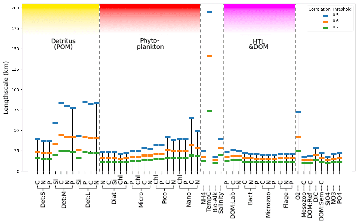
Figure 4 Estimate of mean horizontal length-scales for each ERSEM variable on the shelf (as shown in Fig. 2 for diatoms chlorophyll with a threshold of 0.5) from 300 sample locations, using correlation metrics to determine distance at which mean correlation drops below thresholds of 0.5, 0.6, and 0.7.

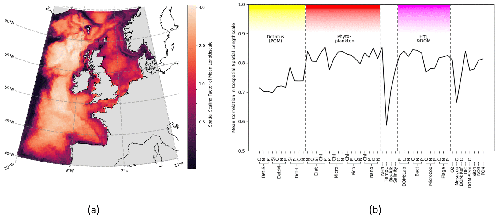
Figure 5 Horizontal length-scales vary spatially across ERSEM variables, using correlation network connectivity to approximate the scaling factor. The spatial variation is consistent between different variables, as shown by the co-spatial Pearson's correlation between each variable. (a) Mean surface length-scale estimates. Average is taken over the full set of ERSEM variables. Correlation threshold is dynamically adjusted for each variable as described in Sect. 3.2.3. (b) Mean Pearson's correlation between co-spatial horizontal length-scales of each variable to every other variable.

Not only is there a large variation in the mean horizontal length-scales between variables (found according to Sect. 3.2.1), but the spatial variation of these length-scales is also hugely significant (as found according to Sect. 3.2.3). This spatial variation is examined in Fig. 5, which shows that, as long as a specific scaling of each variable is taken into account, there is a clear and consistent structure to the significant spatial variation in the horizontal length-scales across the ocean surface. In particular, there is clear similarity in the spatial length-scale distributions between variables, as shown by their high correlation value (R>0.7, Fig. 5b). This indicates that the spatial maps of horizontal length-scales differ between variables mostly by a constant scaling factor shown in Fig. 4. Results in Figs. 4 and 5 suggest that if we write length-scale ℓ as a function of a biogeochemical variable v and spatial location x, i.e. ℓ(v,x), then it can be approximately factorized as a product of two independent functions, i.e. $\stackrel{\mathrm{‾}}{\mathrm{\ell }}\left(v\right),f\left(x\right)$: $\mathrm{\ell }(v,x)\approx \stackrel{\mathrm{‾}}{\mathrm{\ell }}\left(v\right)\cdot f\left(x\right)$. This hugely simplifies the task of attributing horizontal length-scales to new assimilated variables, as the horizontal length-scales can be determined from two independent functions: a variable-dependent mean length $\stackrel{\mathrm{‾}}{\mathrm{\ell }}\left(v\right)$ (Fig. 4) and a dimensionless spatial length-scale variability function f(x) (Fig. 5a). It is worth noting that temperature is the poorest fit to this model, owing to its weak correlation in Fig. 5b, further suggesting that the horizontal length-scales of the biogeochemical variables cannot be easily derived from those of the physical variables.

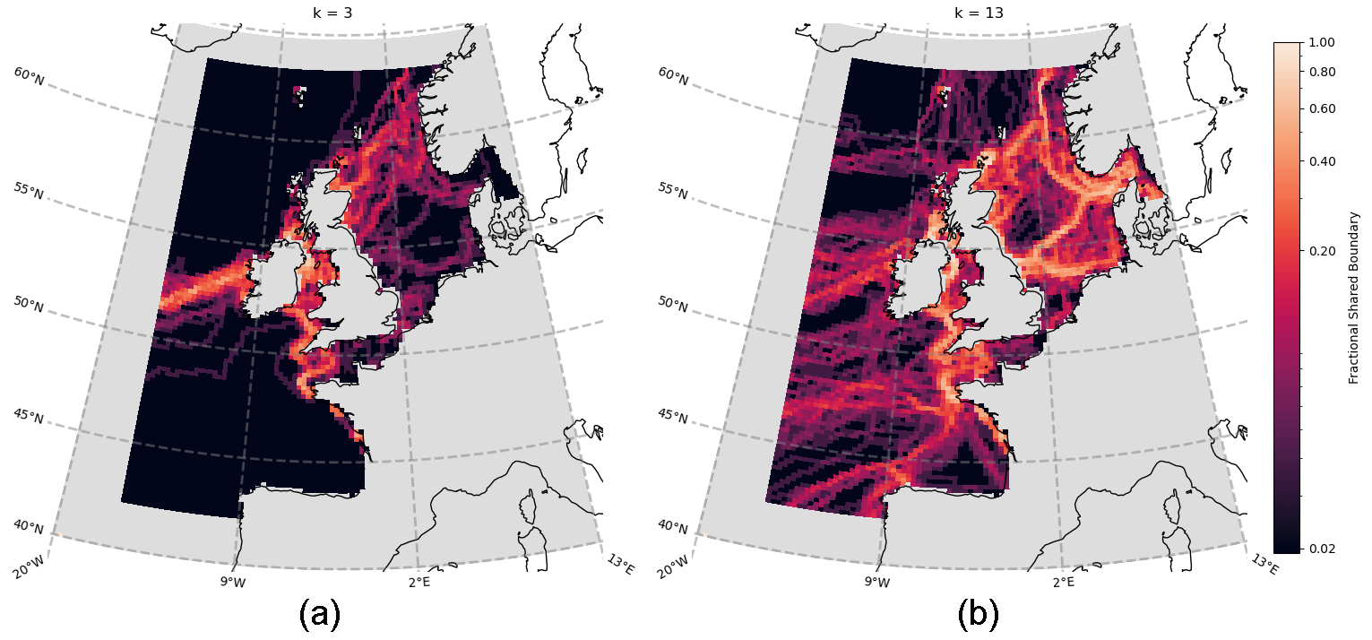
Figure 6 Aggregated boundary heatmap generated from community detection (clustering) of the spatial network for each of the 50 ERSEM variables (cf. Table 1). Points are coloured according to the number of boundaries (as derived from different variables) that intersect, with bright regions indicating that many variables share a boundary and darker regions indicating the absence of many boundaries. Panel (a) shows cluster number k=3, while panel (b) shows k=13.

Beyond the applications in DA, identifying horizontal length-scales is also relevant for the design of appropriate strategies for probabilistic prediction or model error compensation. For instance, when considering how to model stochastic noise across the spatial domain, we can clearly see that simply applying white noise across each grid point would be unrealistic, as there are significant spatial correlations to consider (e.g. applying such noise to and initialization to introduce uncertainty in initial value conditions). As outlined, these spatial correlations will also vary in size, meaning that the correlated noise model should be scaled differently according to the target variable.

Of particular interest in Fig. 5 is that whilst in the majority of the domain the variables are spatially correlated, there are distinctive boundaries or “cuts” (lines of low connectivity) between areas in the domain, where the length-scale decreases rapidly relative to the surrounding areas. The examples of this can be seen along NWES boundaries, such as the Norwegian Trench and the seas north of Scotland, or around some known geographic features, such as the Oyster Grounds. These sharp features with clear interpretation indicate that spatial maps such as Fig. 5a are indeed a robust model representation of the real system in the mixed layer. We would therefore expect any other trustworthy models to produce similar results. These lines of extremely low connectivity mean information is not shared across a given boundary, and the regions within those boundaries instead form their own quasi-self-governing community of behaviour. We shall explore this idea further in Sect. 4.3. It is notable that another area of low connectivity is the open (Atlantic) AMM7 domain boundary regions. This indicates that the boundary conditions of the regional model decorrelate from the rest of the domain. The lack of connection between the boundaries and the rest of the domain can be seen as desirable, considering the large uncertainty in the open boundaries of regional ecosystem models. Because of their uncertainty, we have excluded the boundary regions from any further analyses presented here.

4.2 Regionalization using spectral graph clustering

Figure 6 shows the aggregated community boundaries resulting from the use of spectral graph clustering (SGC; see Sect. 3.3) on the spatial networks of each variable. Every point on the map is coloured according to the number of boundaries that pass through it – meaning the brighter robust boundaries are common to the vast majority (> 75 %) of variables. Conversely, the darker regions indicate areas where fewer (if any) boundaries exist, across all the variables. From Fig. 6a, at a cluster count of only k=3 (see Sect. 3.3), distinct boundaries form across the Atlantic Ocean and the opening to the English Channel and Irish Sea. These lower-order, larger-scale, approximations of the non-shelf boundary areas are consistent with well-known regionalizations such as the Longhurst provinces (Longhurst et al., 1995). We focused then on smaller-scale shelf sea areas. As the number of clusters chosen increases and the domain splits further, the cluster boundaries on the shelf converge onto more intricately shaped and sized real features. This is illustrated in Fig. 6b for the case with k=13 clusters. At these higher cluster counts, it is clear that the variables share large boundaries, particularly on the shelf. This indicates that they are likely a robust feature of the domain (in Fig. 6 they always represent 75 %–100 % of variables). It is important to emphasize that this would not necessarily be the case, as the network construction and regionalization for each variable are independent of each other, which does show through in the form of some less robust boundaries (< 40 % shared) that appear to be subdividing the more robust regions on the shelf.

We used those robust boundaries to identify 13 regions representing areas of NWES connectivity. Results of this regionalization are represented in Fig. 7. It is anticipated that, between the 13, each region identifies areas with similar biogeochemical/ecosystem characteristics within its boundaries. The converse is not necessarily true: two dynamically disconnected regions that communicate little between each other can still have similar characteristics. However, many of the regional boundaries shown in Figs. 6 and 7 clearly match the well-known geographic features of the area, e.g. German Bight, Southern Bight, Dogger Bank, Norwegian Trench, or more broadly the English Channel and North Sea. Our complex network clustering also provides reasonably similar results to the expert-based partition of the NWES applied in many studies (Ostle et al., 2016; Legge et al., 2020; Fowler et al., 2023), with some extra fine details and some new regions included.

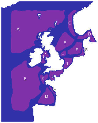
Figure 7 The 13 key regions identified based on the regionalization found in Fig. 6, labelled A–M (purple). Each region aims to cover an area with few intersecting boundaries, without crossing locations with a high number of boundaries. Any area not assigned to one of these regions (blue) is due to uncertainty resulting from either domain boundaries or region boundaries.

While we see that the features from Fig. 6 are at least partly driving the bathymetry of the domain (see Fig. 1), the boundaries particularly seem to reflect a shallower bathymetry (approx. 100 m) than the 200 m depth usually applied to delimit the margins of shelf seas, including the NWES. As a consequence of that, a large section of the NWES near the open ocean boundary (e.g. Celtic Sea, the north-west section of the NWES) is in fact connected to the open ocean and can be seen as an area of robust shelf sea to open ocean exchange. Some regional boundaries reflect the properties of the water column often linked to bathymetry, e.g. the boundaries between regions J and K (Fig. 7) in the western English Channel, and similarly the boundary of region J at the Southern Bight, corresponds to the boundary between the permanently mixed and seasonally/intermittently stratified waters (Ostle et al., 2016). The regions C and D along the Norwegian Trench and G in the German Bight from Fig. 7 are coastal areas influenced by major riverine outflow. The boundaries of those regions effectively delimit the area into which the nutrient- and fresh-water-rich outflow propagates, as a function of local dominant currents. This can be seen in some more detailed plots of chosen ecosystem indicators across the 13 regions from Fig. 7, which can be found in Fig. S1.

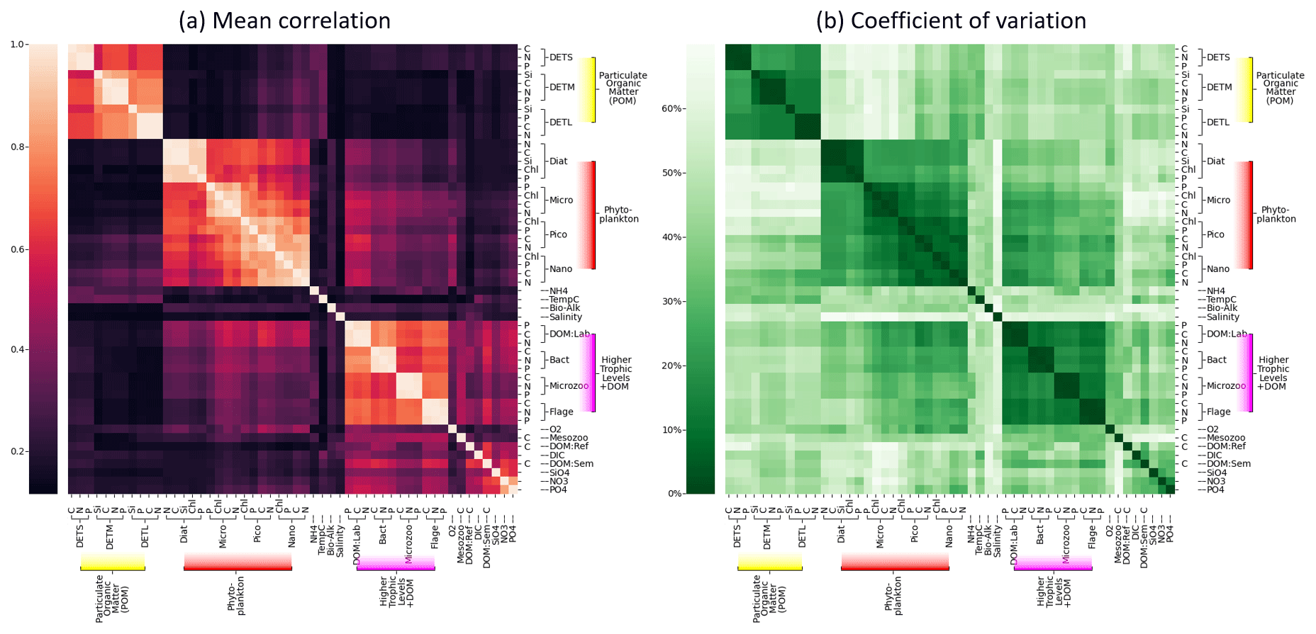
Figure 8 Grouping of ERSEM state variables calculated from 300 sample points on the NWES. Panel (a) shows the mean absolute Spearman correlation between each pair of variables, with the rows and columns sorted using hierarchical clustering, as denoted by the dendrogram. Panel (b) shows the coefficient of variation (Eq. 8) but shown as a percentage, using the same ordering found for panel (a).

4.3 Inter-variable interaction networks

Figure 8 shows sets of ERSEM state variables that behave functionally as groups, together with a confidence measure to ensure these groups are robust and consistent. More specifically, Fig 8a shows mean absolute values of co-spatial Spearman cross-correlations between each pair of biogeochemical variables at 300 sample points on the shelf (bathymetry ≤ 200 m). The diagonal values represent correlations of each variable with itself and are by definition equal to 1. A hierarchical clustering algorithm is applied to this matrix to arrange the variable order, creating groups of similar variables that can be easily identified as distinct blocks of elements that form around the diagonal (Müllner, 2011). Figure 8b shows the corresponding coefficient of variance, Eq. (8), calculated from the same 300 sample points.

If two variables display a high mean correlation and low coefficient of variation, it indicates that there is a reliable and consistent connection between them in the NWES model dataset. The pairwise elements of each group within a high-correlation “block” tend to show a low coefficient of variation in the corresponding plot, indicating that these variables can be grouped together both reliably and consistently.

Although some of these links among variables could have been anticipated to some degree, the quantitative grouping demonstrates the opportunity, and provides the metric, for researchers aiming to either reduce the complexity of the ERSEM ecosystem model or build more simplified (but realistic with respect to the objectives) models than ERSEM. For example, Fig. 8a shows that different biomass components (chlorophyll, carbon, nitrogen, phosphorus, and silicon) of the same phytoplankton type are strongly correlated and grouped together, which means their values can in principle be reasonably predicted from each other. This implies that despite the sources of potentially significant variability in the phytoplankton stoichiometry (e.g. variations in its chlorophyll-to-carbon ratios due to changes in environmental light conditions), Fig. 8 indicates that these are relatively secondary compared to the overall dynamics (growth, grazing, mortality, sinking) governing the phytoplankton biomass. As a result of this, we argue that a simpler model can be formulated by fitting the (potentially non-linear) relationships between the different phytoplankton biomass components and grouping them only into one functional variable. Similarly, another simplification suggested by the connectivity analysis from Fig. 8 is to merge different phytoplankton functional types into one, i.e. mostly the two nanophytoplankton and picophytoplankton species into a single “small-size phytoplankton” functional group, along with the larger diatoms and microphytoplankton groups. Given that the size of the phytoplankton species is known to strongly correlate with various aspects of their dynamics, such as photosynthetic light absorption, metabolic rates, and sinking rates (e.g. the smaller species are more representative of phytoplankton in the open ocean or oligotrophic areas), such groupings arguably reflect the underlying driving physical processes. Besides the phytoplankton functional group, Fig. 8 demonstrates two more clusters of variables: the group of particulate organic matter (POM) and the group consisting of heterotrophic flagellates, microzooplankton, heterotrophic bacteria, and dissolved organic matter (DOM). The links in the latter group are provided through plankton feeding and excreting organic matter. The groups in Fig. 8 correspond well with the ERSEM model functional type diagram (Butenschön et al., 2016) (cf. Table 1); however, their specifics, like the concrete grouping of living and non-living organic matter, are still quite non-trivial.

Finally, we would like to caution against over-interpreting the Spearman cross-correlation matrix from Fig. 8. The matrix shows potentially non-linear connections between variables that could be parameterized, reducing the number of model state variables and replacing a computationally expensive part of the model with cheaper formulations. However, little correlation in the matrix certainly does not imply little dynamical relationship in the model. For example, phytoplankton and nutrients are very strongly dynamically interconnected, but their connection is complex and cannot be expressed as a simple monotonic function captured by the correlation. This demonstrates itself by different signatures of correlation coefficient at different times; for example, at times when nutrients are a limiting factor to phytoplankton growth, phytoplankton and nutrients will be positively correlated, whereas if the nutrients are reduced through uptake they will be negatively correlated with phytoplankton.

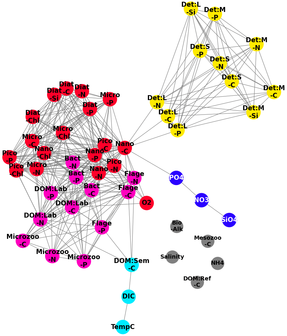
Figure 9 A network derived from the correlation measures found in Fig. 8, where we treat the pairwise correlations as an adjacency matrix and apply a spectral clustering algorithm to partition the variable set into functional groups, denoted by the colours: red (phytoplankton), yellow (detritus), cyan (DOM:Sem-C, DIC and TempC (temperature in degrees Celsius. )), blue (SiO₄, NO₃, PO₄), pink (HTL (higher trophic levels ) and DOM), and grey (Salinity, Mesozoo-C, DOM:Ref-C, NH₄, Bio-Alk). The highest correlations (top 25 %) of all possible pairwise correlations between variables are shown (grey lines).

Figure 8 can be naturally interpreted in the context of complex network analysis, by considering panel (a) as an adjacency matrix of a network. In this instance, the nodes are the variables and the links are determined by the top 25 % most robust correlations. To identify the functional groups behind the biogeochemistry variables, we applied SGC (as described in Sect. 3.3 and 3.4, for $\mathrm{1}\le k\le \mathrm{20}$, with k=5 giving the most interpretable results) to the cross-correlation matrix from Fig. 8a, and the results are displayed in Fig. 9. Three main groups identified from the correlation matrix are clearly visible: particulate organic matter (yellow), phytoplankton (red), and the cluster of higher-trophic-level variables and DOM (pink). The blue cluster consists of nitrates, phosphates, and silicates (the nutrients), and it is only weakly connected to the rest of the network. As already mentioned, being “weakly connected” does not necessarily imply a lack of dynamical connection; it may mean the connection is too complex to be parameterized by a monotonic function. The observed links in Fig. 9 between the nutrients (nitrates, phosphates, silicates) can be explained through the observed links between the different plankton/POM/DOM chemical elements represented by the model (carbon, nitrogen, phosphorus, silicon). These links suggest there is a high degree of connection between the different element cycles. The connection between element cycles then naturally implies connection between the elements also in their inorganic (nutrient) form. However, there is additional complexity: the inorganic form of nitrogen is represented in the model by both ammonium and nitrates, which are related through the process of nitrification. Ammonium is not only involved in phytoplankton assimilation and nitrification (as nitrate) but also in phytoplankton excretion and remineralization of organic matter by bacteria. Ammonium also drives changes in bio-alkalinity. This additional complexity might be behind the fact that ammonium is not part of the “nutrients” cluster but is separated from all the other variables (Fig. 9).

The cyan cluster consists of temperature, dissolved inorganic carbon (DIC), and semi-labile organic matter, with the dissolved inorganic carbon being weakly connected to the higher-trophic-level–DOM cluster. Connections between temperature and gases, such as CO₂, which form the majority of the DIC, are explained by the fact that temperature drives gas solubility in the water. However, such connections do not always happen on the timescale relevant to this analysis; for example, oxygen is not found to be part of the cyan cluster. This can in part be explained by the longer (∼ 2–3 weeks) timescale on which sea surface temperature (SST) drives near-surface oxygen on the NWES (Skákala et al., 2023). Crucially, on the shorter timescales analysed in this study, oxygen is more strongly linked to the phytoplankton group (Fig. 9) through photosynthesis and respiration. Finally, there are several variables (e.g. salinity or, as we previously mentioned, ammonium) coloured in grey that are completely disconnected from the rest of the network.

5 Conclusions

Marine biogeochemistry is complex to simulate, representing a plethora of processes in an often computationally costly manner. As a result, it is not well suited for addressing specific questions that necessitate extensive and long-lasting ensemble simulations, such as ecosystem response to climate change and anthropogenic stresses across a broad range of scenarios, or analyses aimed at informing policy-making decisions. Here, we aimed to use a complex network analysis to gain insight into connections found across the ecosystem while providing an understanding that will aid in the simplification of its complex interactions and dynamics.

With future observation missions that will provide new biogeochemical variables for assimilation, there is a need to further understand how transferable the spatial horizontal correlation length-scales are between the different biogeochemical variables. Using the correlation analysis and the resulting spatial networks, we can conclude that the biogeochemical horizontal correlation length-scales at the ocean surface vary significantly between variables and are not directly transferable. However, we have provided an approximation for the horizontal correlation length-scales of all variables across the whole NWES spatial domain. The spatial horizontal correlation length-scales are derived for the ocean surface but are expected to be relevant within the ocean mixed layer. The spatial length-scale distributions are similar (highly correlated) across the variables and form realistic spatial features, enhancing the confidence in those results. With this clear indication of structure embedded into the horizontal connectivity of the ecosystem, we sought to split the shelf sea into geographic regions using clustering network algorithms. This clustering process was applied to each variable independently, yet it identified a set of clear and consistent boundaries that represent areas of extremely low connectivity across which information is not shared. This resulted in 13 key regions, suggesting that each functions as a quasi-separate system but with unified biogeochemical/ecosystem characteristics within its boundaries. This also identified the Celtic Sea and the north-west section of the NWES as areas of high exchange between the shelf sea and open ocean. Finally, we demonstrated that the complex network carries important information on how the ecosystem variables cluster into natural functional groups. Our analysis demonstrated that the chemical components (nitrogen, carbon, silicon, etc.) of each pelagic variable (e.g. diatoms, nanophytoplankton, microzooplankton) are closely linked, and a simpler version of the model can be built, by reducing these variables through parameterization. We also see that the pelagic variables form even larger functional groups (e.g. POM, phytoplankton, HTL/DOM), composed of variables that can be effectively parameterized through monotonic functions of each other.

These findings show that complex networks can be used as an effective tool in simplifying the complexity of the ecosystem dynamics, providing simplifications to the system extracted from the behaviour of the model itself. These simplifications will be applied in future work, e.g. building an ML-based reduced-order emulator to improve data assimilation on the NWES.