the Creative Commons Attribution 4.0 License.
the Creative Commons Attribution 4.0 License.
 | 16 Feb 2024
Multiscale assessment of North American terrestrial carbon balance
Kelsey T. Foster
Yoichi P. Shiga
Jiafu Mao
Anna M. Michalak
Comparisons of carbon uptake estimates from bottom-up terrestrial biosphere models (TBMs) to top-down atmospheric inversions help assess how well we understand carbon dioxide (CO2) exchange between the atmosphere and terrestrial biosphere. Previous comparisons have shown varying levels of agreement between bottom-up and top-down approaches, but they have almost exclusively focused on large, aggregated scales (e.g., global or continental), providing limited insights into reasons for the mismatches. Here we explore how consistency, defined as the spread in net ecosystem exchange (NEE) estimates within an ensemble of TBMs or inversions, varies with at finer spatial scales ranging from to the continent of North America. We also evaluate how well consistency informs accuracy in overall NEE estimates by filtering models based on their agreement with the variability, magnitude, and seasonality in observed atmospheric CO2 drawdowns or enhancements. We find that TBMs produce more consistent estimates of NEE for most regions and at most scales relative to inversions. Filtering models using atmospheric CO2 metrics causes ensemble spread to decrease substantially for TBMs, but not for inversions. This suggests that ensemble spread is likely not a reliable measure of the uncertainty associated with the North American carbon balance at any spatial scale. Promisingly, applying atmospheric CO2 metrics leads to a set of models with converging flux estimates across TBMs and inversions. Overall, we show that multiscale assessment of the agreement between bottom-up and top-down NEE estimates, aided by regional-scale observational constraints is a promising path towards identifying fine-scale sources of uncertainty and improving both ensemble consistency and accuracy. These findings help refine our understanding of biospheric carbon balance, particularly at scales relevant for informing regional carbon-climate feedbacks.
- Article
(1933 KB) - Full-text XML
-
Supplement
(1723 KB) - BibTeX
- EndNote


Reliable estimates of carbon dioxide (CO2) uptake by the terrestrial biosphere are necessary for understanding both historical and future climate change because the terrestrial biosphere mitigates anthropogenic CO2 emissions by storing carbon in above- and below-ground biomass. Net ecosystem exchange (NEE) of CO2 cannot be measured directly at scales greater than a plot (∼ 1 km2); that is, the scale of the footprint of an eddy covariance flux tower (Kljun et al., 2015). Estimates at broader scales therefore rely either on “bottom up” methods such as terrestrial biosphere models (TBMs) that represent process-based understanding of flux drivers (e.g., Hayes et al., 2012; Sitch et al., 2015) or on “top down” methods such as atmospheric inverse models that attribute observed atmospheric variability in CO2 concentrations to upwind biospheric activity (e.g., Ciais et al., 2011; Gourdji et al., 2012; Gurney et al., 2002; Michalak et al., 2004; Peylin et al., 2013; Shiga et al., 2018a; Thompson et al., 2016).
Understanding of net biospheric carbon uptake has improved through comparisons between TBMs and inversions (Hayes et al., 2012; King et al., 2015), but discrepancies both between these approaches and between specific models using either approach have persisted even in relatively well studied regions such as North America and Europe. The resulting uncertainties in carbon flux estimates limit our ability to anticipate carbon–climate feedbacks, and therefore to assess the impacts of alternative emission pathways and related climate mitigation policies (Friedlingstein et al., 2014; Huntzinger et al., 2017; King et al., 2015). Uncertainties both between modeling approaches and between specific models arise from the specific characteristics of TBMs and inversions.
For TBMs, model performance is limited by incomplete understanding of underlying processes (Hayes et al., 2012; Huntzinger et al., 2012, 2017; Schwalm et al., 2010, 2019; Seiler et al., 2022). One major source of uncertainty is that models may incorporate different key mechanisms or represent them with varying levels of detail. For example, nitrogen limitation likely reduces CO2 fertilization, but coupled carbon–nitrogen dynamics are not included in all models (Bonan and Levis, 2010; Brovkin and Goll, 2015; Jain et al., 2009; Sokolov et al., 2008; Tharammal et al., 2019; Thornton et al., 2009; Wieder et al., 2015), and permafrost thaw, which can cause release of carbon from high latitudes (Burke et al., 2013; Koven et al., 2013), is not mechanistically resolved in most models. Large discrepancies also arise from different approaches to modeling land use change, vegetation dynamics, and fire (Ahlström et al., 2015; Bastos et al., 2020; Hardouin et al., 2022; Tharammal et al., 2019). Beyond such structural uncertainties, models parameterize processes differently and often use different driving data, which introduces additional uncertainty (Huntzinger et al., 2017; Jung et al., 2007; Lovenduski and Bonan, 2017; Schwalm et al., 2010, 2019). Previous studies have addressed the use of different driver data by establishing model ensembles that adhere to a standardized protocol and utilize consistent forcing data, but doing so does not fully account for observed uncertainties (Huntzinger et al., 2013, 2020; Friedlingstein et al., 2020; Sitch et al., 2015). Understanding and addressing these key sources of uncertainty in TBMs helps to improve our understanding of biospheric carbon exchange
For inversions, uncertainties arise from the limited information content of available atmospheric observations and from choices made in the statistical setup of the model. More specifically, the choice of prior estimates, prior error correlations, observational data, transport model, boundary conditions, data assimilation time period, and model resolution all lead to differences across models (Ciais et al., 2010; Göckede et al., 2010; Kondo et al., 2020; Michalak et al., 2017; Peylin et al., 2013). Paradoxically, even regions with relatively high data availability, such as Europe, can still exhibit large spread in carbon uptake estimates derived from inverse models (Kondo et al., 2020; Monteil et al., 2020). This suggests that other aspects of the inverse modeling framework may be more significant contributors to uncertainty, though there is not a clear consensus on the main source of uncertainty (Gaubert et al., 2019; Kondo et al., 2020). For example, some studies have found transport errors to be a primary source of uncertainty (Peylin et al., 2013; Schuh et al., 2019), while other studies have shown that fossil fuel emission uncertainties play a key role in variability (Gurney et al., 2005; Peylin et al., 2011; Saeki and Patra, 2017). Another limitation is that atmospheric CO2 observations, and inversions based on these observations, do not directly inform process-level understanding of the controls on carbon uptake to the extent that bottom-up approaches can (Baker et al., 2006; Gurney et al., 2004).
Given the uncertainties inherent to both approaches and their complementary strengths, comparisons between ensembles of TBMs and inversions can be particularly helpful in diagnosing our understanding of the carbon balance of the terrestrial biosphere. If TBMs and inversions yield similar estimates, this agreement increases confidence in the reliability of both model types as sources of realistic information. Previous studies, however, have come to different conclusions about the degree of agreement between bottom-up and top-down estimates (Bastos et al., 2020; Canadell et al., 2011; Kondo et al., 2020; Hayes et al., 2018). Some comparisons have shown agreement between NEE estimates from TBMs and inversions (Ciais et al., 2010; King et al., 2015; Sitch et al., 2015), while others have shown a large amount of variability both within and between bottom-up and top-down ensembles (Bastos et al., 2020; Chevallier et al., 2014; Huntzinger et al., 2012, 2017; Schwalm et al., 2019; Sun et al., 2021). For instance, King et al. (2015) found bottom-up and top-down methods agree on the sign of the North American land sink, albeit with notable spread in estimates, while Kondo et al., found bottom-up and top-down approaches disagree in many countries at the regional scale. Furthermore, Chevallier et al. (2014) showed that an ensemble of inversions had significant disagreement at the hemispheric and regional scales and Huntzinger et al. (2012) reported a lack of consensus among TBMs in determining whether North American land functions as a carbon sink or source.
A common approach for comparing TBMs and inversions is to examine the agreement across the mean of model ensembles (Ciais et al., 2010; Hayes et al., 2012; King et al., 2015). Here we use the term “agreement” between estimates to refer to the degree to which NEE estimates from an ensemble of TBMs differ from NEE estimates from an ensemble of inversions. In addition, analyzing the variability or spread amongst TBMs or inversions provides insights into the degree of consistency in carbon flux estimates. Here we use the term “consistency” of estimates to refer to the degree of variability in NEE estimates within an ensemble of either TBMs or of inversions.
Previous comparisons between bottom-up and top-down estimates have revealed that the agreement between estimates depends on the spatial scale and the region. At the global scale, inversions yield more consistent NEE estimates than TBMs (Friedlingstein et al., 2022), largely due to the global constraint provided by atmospheric CO2 observations. However, at regional scales, consistency is limited for both TBMs and inversions and it is even difficult to determine whether certain regions are a net sink or source of CO2 (Ciais et al., 2013; Kondo et al., 2020) due to the uncertainties associated with both approaches outlined above. For North America, agreement between bottom-up and top-down estimates has improved over time, but this apparent agreement is in part due to the large range of estimates (i.e., low consistency) for both TBMs and inversions (Hayes et al., 2012; King et al., 2012, 2015; Pacala et al., 2001). This scale- and region-dependent agreement makes it difficult to determine the optimal path towards reducing uncertainties. This challenge is in part because comparisons of bottom-up and top-down methods are primarily conducted at large aggregated scales – for example, global, hemispheric, and continental scales (Bastos et al., 2020; Ciais et al., 2010; Hayes et al., 2012; Huntzinger et al., 2012; Pacala et al., 2007; Peylin et al., 2010), which aids little in attributing causes of observed mismatches (Bastos et al., 2020; Hayes et al., 2012; Kondo et al., 2020).
A key step forward is to look at agreement beyond large, aggregated scales. Looking across multiple spatial scales provides a more in-depth understanding of the level of agreement between carbon budgets from bottom-up and top-down approaches. Despite this, few studies have taken this approach, especially for sub-continental spatial scales. Agreement between bottom-up and top-down estimates at global and hemispheric scales (Bastos et al., 2020; Kondo et al., 2020; Sitch et al., 2015) is a necessary but not sufficient condition for reconciling differences in carbon budgets at regional scales (Kondo et al., 2020). When large spread in model estimates makes it difficult to determine whether large regions such as Europe, boreal Asia, Africa, South Asia, and Oceania are even net sinks or sources (Kondo et al., 2020), multiscale comparisons may shed new light on the lack of consistency. Gourdji et al. (2012) compared bottom-up and top-down models at sub-continental scales and found better agreement during the growing seasons than in the dormant season, allowing for a more in-depth and focused exploration into the reasons for the observed (dis)agreement. The key insights gained from multiscale comparisons highlight the need for a more comprehensive comparison of bottom-up and top-down NEE estimates across spatial scales (Gourdji et al., 2012; Kondo et al., 2020).
Examining the agreement between bottom-up and top-down methods across spatial scales can also provide insights into the relationship between consistency, agreement, and accuracy in model predictions. Assessing agreement between bottom-up and top-down budget estimates is not necessarily equivalent to determining the accuracy of carbon budgets, however (Knutti et al., 2010; Kondo et al., 2020; Lovenduski and Bonan, 2017). Instead, accuracy should be assessed against observational constraints. There have been efforts, such as the International Land Model Benchmarking Project (ILAMB), to evaluate model accuracy by quantifying agreement between reference datasets and model outputs across multiple statistical metrics (Collier et al., 2018). Model skill scores are useful in assessing agreement between reference data and model data, but it is possible to misinterpret model performance without careful analysis of the metrics that make up the overall skill score (Bonan et al., 2019; Collier et al., 2018). In addition, reference data to which models are compared are often themselves modeled data products (e.g., FLUXCOM is used as reference data for gross primary productivity (GPP); Seiler et al., 2022). Model evaluation against atmospheric CO2 observations can in principle provide more direct insights into the variability and accuracy of model NEE estimates (Fang et al., 2014; Fang and Michalak, 2015; Sun et al., 2021). By comparing carbon budget estimates to atmospheric CO2 observations, in addition to comparing these estimates across spatial scales, we can determine the degree to which consistency within an ensemble is representative of accuracy. While better model performance under current conditions does not necessarily indicate better performance under future conditions, this approach helps with model improvement by allowing for quick identification of which models yield more realistic results. Subsequently, in-depth analysis can be done to identify key model characteristics that lead to improved results.
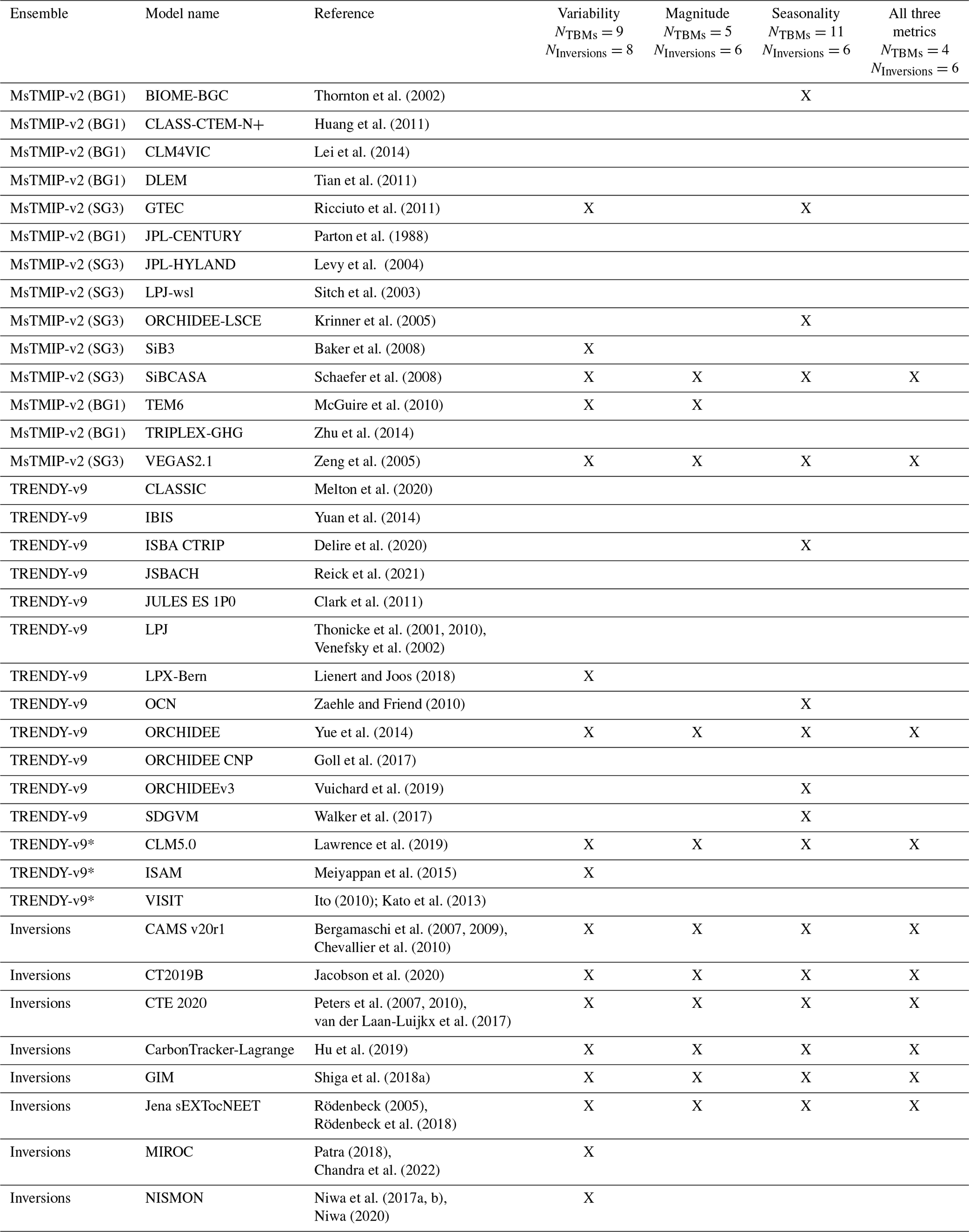
Here, we compare large ensembles of bottom-up and top-down model estimates of NEE for North American across various spatial scales to assess how consistency in model estimates varies across scales and between modeling approaches (Table 1). We expect inversions to be more consistent at larger scales thanks to the constraint provided by atmospheric observations, and TBMs to be more consistent at smaller spatial scales because they are informed by process-based understanding. We then evaluate whether greater consistency corresponds to higher accuracy and lower uncertainty in overall NEE estimates. We determine if the consistency within ensembles and the agreement between top-down and bottom-up approaches are impacted by ensemble subsetting; that is, limiting ensembles to models that can reproduce basic aspects of the variability, magnitude, and seasonality of atmospheric CO2 observations. We expect consistency to improve when ensembles include only models that agree with basic features of atmosphere CO2 observations, thereby also increasing the degree to which consistency informs accuracy, or, in other words, making model spread a more apt measure of uncertainty.
Table 1Names and references for the models included in each ensemble used in this study. The models that meet the variability, seasonality, magnitude, or all three metrics are indicated by an “X”. An asterisk indicates the models that were present in MsTMIP-v2 (CLM4 BG1, ISAM BG1, and VISIT SG3) but are replaced by updated versions in TRENDY-v9; in this case the metrics were evaluated based on TRENDY-v9 versions (see Sect. 2.1.1), but the MsTMIP-v2 versions were used when evaluating the impact of how NEE is defined on consistency and agreement (Sects. 3.1 and 3.3.3, Fig. S7).
2.1 Data
2.1.1 Model ensembles
Estimates of NEE from three model ensembles were used (Table 1). Bottom-up estimates came from two TBM intercomparison projects, namely, the Multi-scale Synthesis and Terrestrial Model Intercomparison Project (MsTMIP-v2; Huntzinger et al., 2013, 2018, 2021; Wei et al., 2014a, b) and the Trends in Net Land-Atmosphere Exchange version 9 ensemble (TRENDY-v9; Friedlingstein et al., 2020; Sitch et al., 2015). MsTMIP is a model intercomparison project aimed at exploring the impact of structural differences in models by prescribing a fixed protocol with a semi-factorial design and consistent environmental driver data for an ensemble of models (Huntzinger et al., 2013, 2018, 2021; Wei et al., 2014a, b). We use the SG3 and BG1 simulations from MsTMIP-v2, where atmospheric CO2 and land-use history are time-varying and nitrogen deposition rates are held constant in SG3, and land-use history, atmospheric CO2, and nitrogen deposition are time-varying in BG1 (Table 1). MsTMIP-v2 defines NEE to be NEE = Rh+ Ra+ Fdisturbance+ Fproduct− GPP where Rh is heterotrophic respiration, Ra is autotrophic respiration, Fdisturbance is the sum of fire and land use change fluxes, and Fproduct is the decay of harvested wood products. Some models do not include fire, land use, and/or product fluxes, depending on the processes that are represented by the models. TRENDY includes simulations from an ensemble of dynamic global vegetation models (DGVMs) that are run annually as part of the Global Carbon Project yearly evaluation. TRENDY also includes a set of factorial simulations for the historical period (Friedlingstein et al., 2022). Here we use the S3 simulation from TRENDY-v9 where CO2, climate, and land use forcings are time-varying. TRENDY defines NEE as NEE = Rh+ Ra+ Ffire+ Fharvest+ Fgrazing+ FLUC – GPP, where Ffire are emissions from natural and human-sparked fires, Fharvest is emissions from crop harvest, Fgrazing are fluxes from livestock grazing, and FLUC are fluxes resulting from land use change. Models within TRENDY-v9 vary in terms of which components are included. We detail the impact of varying NEE definitions in bottom-up models on our results in Sect. 3.1. Top-down estimates come from a set of inverse model estimates assembled in support of the REgional Carbon Cycle Assessment and Processes 2 (RECCAP-2) analysis (Ciais et al., 2022). RECCAP-2 is a project aimed at quantifying carbon budgets on regional scales across the globe.
For assessing consistency and agreement at biomes scales we use the same biome map as Shiga et al. (2018b) and Sun et al. (2021) that is based on an International Geosphere-Biosphere Programme (IGBP) land cover classification map. MsTMIP-v2 imposes a consistent biome map for all models (Wei et al., 2014a), while models from TRENDY-v9 use various sets of plant functional types (PFTs), resulting in differences in land cover representations (Seiler et al., 2022). While the TRENDY-v9 models have differences in land cover representation, they do use common land use and land cover change (LULCC) forcing data (Seiler et al., 2022). Though using the same biome map across all models would allow for greater standardization amongst TBMs, doing so is difficult due to model-specific setups. Understanding the impact of the various maps used by models is also difficult as few models provide outputs at the resolution necessary to do a comprehensive analysis, such as evaluating whether specific PFTs are present at in situ observation sites (Seiler et al., 2022). However, Sun et al. (2021) did compare the impact of model-specific biome classifications for four models that provided PFT information at finer resolutions and showed that model-specific biome classification was not a primary driver of inter-model variability.
All models were re-gridded to a spatial and monthly temporal resolution and then cropped to a uniform North American domain for the study period of 2007–2010. We correct the CLM5.0 timestamp to address an error causing output files to have a start date shifted by 1 month (ESDS 0.1 documentation FAQ, 2024). For TBMs, only land fluxes are included in model output files and thus ocean grid cells are removed prior to regridding. This period was chosen because this was the time frame for which all models overlapped temporally (until 2010) and during which high-resolution atmospheric transport footprints (see Sect. 2.3) were available (starting in 2007) to link model estimates to atmospheric CO2 observations. We use the model ensemble average when assessing agreement between bottom-up and top-down model ensembles. While this is a simple approach, Schwalm et al. (2015) found that the added complexity of skill-based integration does not materially change flux estimates based on TBM ensembles. The model simulations from MsTMIP-v2 and TRENDY-v9 ensembles were merged to create one TBM superensemble. Because MsTMIP-v2 and TRENDY-v9 have three models in common (CLM, ISAM, and VISIT; Table 1), the simulations from these models included in TRENDY-v9 were used in this analysis because TRENDY-v9 has more recent updates to models than MsTMIP-v2 (e.g., CLM5.0 vs. CLM4).
2.1.2 Atmospheric CO2 observations
Atmospheric CO2 observations are from ObsPack CO2 GLOBALVIEWplus v3.2 (Cooperative Global Atmospheric Data Integration Project, 2017; Masarie et al., 2014) wherein continuous in situ observations were averaged to three-hourly averaged CO2 measurements. Averaging is centered at 15:00 local time for most sites and 16:00 or 17:00 for a few sites; these times were chosen because afternoon observations are expected to have lower transport model errors stemming from model representation of planetary boundary layer dynamics (Lin et al., 2017). Urban sites were excluded as this analysis focuses on the biospheric signal. From the 44 continuous-monitoring towers for the 2007–2010 period selected here, there are around 57 700 available mid-afternoon observations, among which around 39 300 observations were used in the analysis and around 18 400 (32 %) observations were filtered out (Table S1). Data with extreme outliers and CO2 enhancements above 30 ppmv are filtered out as described in Fang and Michalak (2015). In addition, data that have a large sensitivity to ocean fluxes (Gourdji et al., 2012) and data with potential transport model errors are also filtered out (Gourdji et al., 2012; Shiga et al., 2018a).
To isolate the biospheric enhancement or drawdown, background CO2 values and signals from fossil fuel emissions were pre-subtracted. The impact of fossil fuel emissions on available CO2 observations was calculated using footprints from a Lagrangian atmospheric transport model (see Sect. 2.3) and emissions from the Fossil Fuel Data Assimilation System (FFDAS v2; Asefi-Najafabady et al., 2014), scaled to spatial resolution and three-hourly temporal resolution to be consistent with the setup of atmospheric transport. The background CO2 values (or boundary conditions) were calculated similarly to Jeong et al. (2013), where vertical profiles from aircraft data and marine boundary layer data are used to run back trajectories and the endpoints of the back trajectories are sampled to obtain background CO2 values. Overall, data processing and filtering were done in a similar manner to Shiga et al. (2018a) and Sun et al. (2021).
2.1.3 Absorbed photosynthetically active radiation
We use absorbed photosynthetically active radiation (APAR) as a baseline for assessing model performance. APAR is a first-order driver of gross primary productivity (GPP) (Monteith, 1972). We chose to use APAR as opposed to a GPP product, such as MODIS GPP, because we wanted to use the simplest data-driven baseline possible. We view APAR as a simple and more direct baseline than MODIS GPP because MODIS GPP itself is modeled using multiple parameters and is therefore itself a type of model (Running and Zhao, 2015). Because NEE is the balance between GPP and ecosystem respiration, and ecosystem respiration is highly correlated with GPP (Janssens et al., 2001; Baldocchi, 2008), we expect APAR to explain a portion of the variability in NEE. Given that remotely sensed APAR in and of itself does not incorporate biochemical processes governing gas exchange, which are commonly represented in TBMs, we would therefore expect models to outperform APAR in explaining observed variability in atmospheric CO2 concentrations. APAR is calculated as the product of MODIS fAPAR (Myneni et al., 2002, 2015) and photosynthetic active radiation (PAR) following Sun et al. (2021). PAR is calculated by rescaling shortwave radiation from the North American Regional Reanalysis dataset (Mesinger et al., 2006) following the empirical relationship from Meek et al. (1984).
2.1.4 Flux tower NEE
We qualitatively compared FLUXNET2015 NEE with modeled NEE estimates. FLUXNET2015 is a global data product for eddy covariance measurements of carbon, water, and energy exchange between the atmosphere and biosphere (Pastorello et al., 2021). We used the NEE data product with the variable USTAR threshold (VUT), where USTAR (i.e., friction velocity) thresholds vary yearly. We used data from five flux tower locations that are within the same grid cell as towers from ObsPack CO2 GLOBALVIEWplus v3.2 that are used to evaluate seasonality (see Sect. 2.3). The three flux towers located in the same grid cell as the AME tower (Mead, Nebraska; Miles et al., 2012) are located at the University of Nebraska Agricultural Research and Development Center near Mead, Nebraska. The three sites are an irrigated continuous maize site (US-Ne1; Suyker, 2016a), an irrigated maize–soybean rotation site (US-Ne2; Suyker, 2016b), and a rainfed maize–soybean rotation site (US-Ne3; Suyker, 2016c). The two flux towers located in the same grid cell as the LEF tower (Park Falls, Wisconsin; Andrews et al., 2014) are Park Falls (US-Pfa; Desai, 2016a) and Willow Creek (US-WCr; Desai, 2016b), Wisconsin. Given the scale mismatch between the footprint of flux tower observations (∼ 1 km2) and the resolution of the models examined here (), comparisons are only interpreted qualitatively.
2.2 Determining consistency across spatial scales
Bottom-up and top-down NEE estimates are compared to determine which modeling approach provides the more consistent estimate at various spatial scales. Consistency is quantified as the standard deviation across model estimates in the ensemble of TBMs and across the ensemble of inversions. We assess consistency at nested scales of , , , , and for all grid cells throughout the North American domain by first calculating the area-weighted average NEE for each model within an ensemble and then calculating the ensemble standard deviation at each scale (Figs. 2, S1). We also assess consistency at the biome and continental scale. We then compare the consistency of TBMs to that of inversions at each scale to determine whether the more consistent approach is scale-dependent. We use an F test to determine whether differences in consistency between the two ensembles is statistically significant (p<0.05).
2.3 Evaluation against atmospheric observations
We assess the degree to which model-simulated NEE estimates can reproduce basic aspects of observed atmospheric CO2 concentrations using three sets of metrics focusing on variability, magnitude, and seasonality. We compare observed atmospheric CO2 concentrations with modeled CO2 concentrations for all models in the TBM and in the inversion ensembles.
The sensitivity of CO2 enhancements at available observation locations and times to upwind fluxes (ppm [µmol m−2 s−1]−1) are represented using the Stochastic Time-Inverted Lagrangian Transport (STILT) model (Lin et al., 2003; Nehrkorn et al., 2010) driven by meteorological fields simulated by the Weather Research and Forecasting (WRF) model (Skamarock and Klemp, 2008) for North America and aggregated to a spatial resolution and three-hourly temporal resolution. Footprints were generated as part of the NOAA CarbonTracker-Lagrange regional inverse modeling framework (Hu et al., 2019; https://gml.noaa.gov/ccgg/carbontracker-lagrange/, last access: 29 November 2023). The footprints used here cover the time period of 2007–2010. The WRF-STILT model has been previously used to assess TBM estimates of CO2 fluxes (Fang et al., 2014; Fang and Michalak, 2015; Sun et al., 2021) and to quantify greenhouse gas fluxes (Gourdji et al., 2012; Jeong et al., 2013; Miller et al., 2014; Shiga et al., 2018a). Here we use the footprints to translate the space–time patterns of carbon fluxes into their impacts on atmospheric CO2 observations in order to assess the model estimates' ability to represent specific aspects of atmospheric CO2 variability in space and time.
We use the coefficient of determination (R2) between observed and modeled CO2 drawdowns or enhancements as the metric for explained variability, i.e., quantifying the degree to which model estimates can reproduce observed spatiotemporal variability across all observation locations and times. We use the transported signal based on spatiotemporal variability in APAR as a lower benchmark for model performance (see Sect. 2.1.3). If a model has an R2 value that is lower than APAR's R2 value, then that model is removed from the ensemble when this metric is applied (Fig. S2).
Similarly, we use the root mean squared error (RMSE) between observed and modeled CO2 drawdowns or enhancements as the metric for the magnitude of CO2 signals from modeled fluxes. We again use APAR as a lower benchmark, but in this case, we first rescale APAR by minimizing RMSE. This step comes down to performing a linear regression between the transported APAR signal and the observed CO2 enhancements, which also implicitly embodies the necessary unit conversion. If a model has a higher RMSE than that of the rescaled APAR signal, then that model is removed from the ensemble when this metric is applied (Fig. S3).
We use four sub-metrics to assess seasonality. Seasonality is assessed at individual towers that have CO2 concentration observations for at least 50 % of days in the study period and for which the maximum data gap is less than 31 consecutive days. Only four towers within our study region meet these criteria (red symbols in Fig. 1): LEF (Park Falls, Wisconsin, USA), AME (Mead, Nebraska, USA), WKT (Moody, Texas, USA), ETL (East Trout Lake, Saskatchewan, Canada). The towers included in this analysis fall within different biomes and have different average seasonal cycles, allowing for assessment of agreement between modeled and observed CO2 seasonal cycles across various landscapes. We also conducted a sensitivity analysis to test if the number of towers used for the seasonality metric has a significant impact on model selection. To do so, we relaxed the criteria for tower selection to a maximum allowable data gap of 80 consecutive days yielding four additional towers: SGP (Southern Great Plains, OK, USA), AMT (Argyle, ME, USA), OFR (Fir, OR, USA), and EGB (Egbert, ON Canada) (see Fig. S4). We calculate the monthly average observed and modeled CO2 seasonal cycle for each of these four towers across the four years (2007–2010).
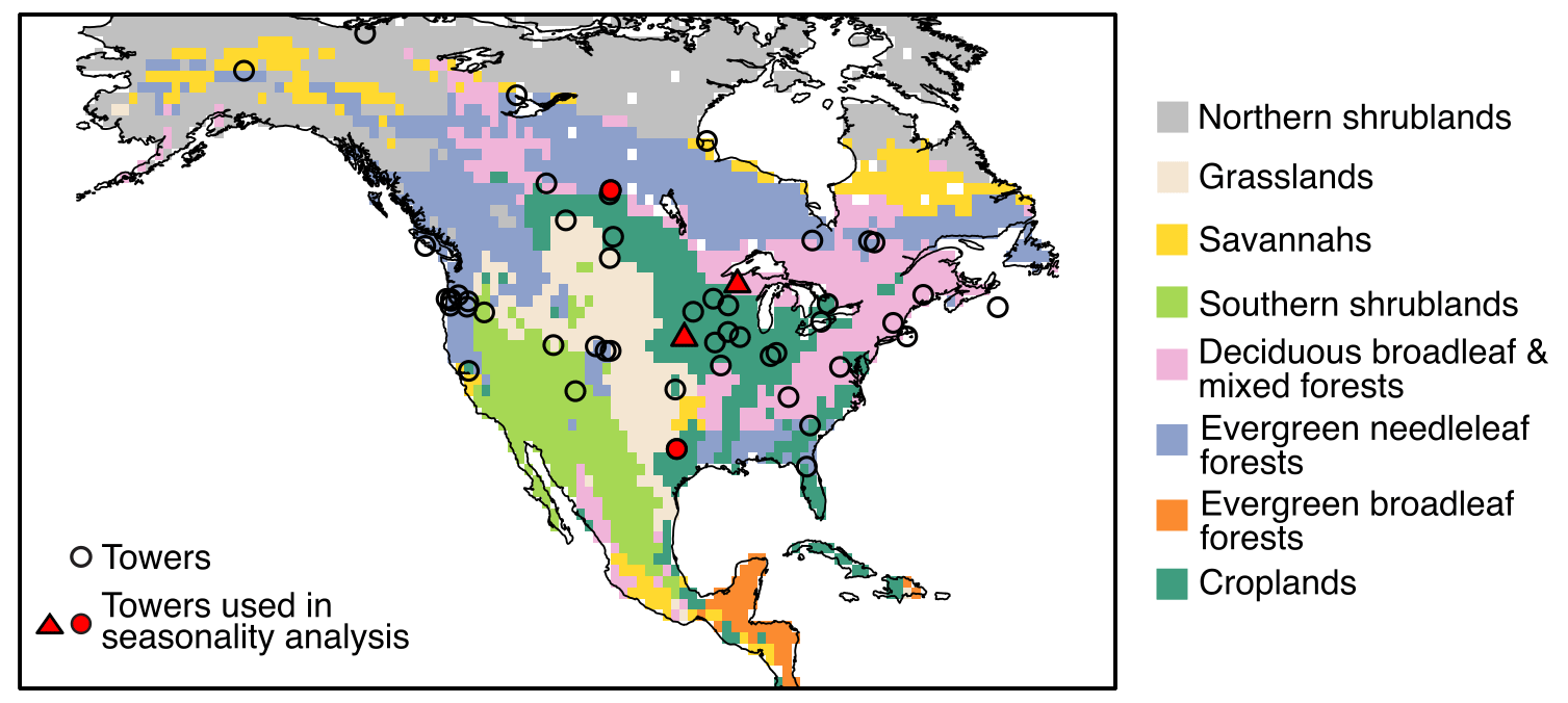
Figure 1Map of biomes in North America with the locations of continuous-monitoring towers used in this study. Symbols represent the locations of towers in the CO2 observational network. Red filled symbols represent the subset of towers with high temporal coverage that were used to evaluate how well model-simulated NEE estimates reproduce the seasonality of atmospheric CO2 observations, whereas all towers are used for the magnitude and variability metrics (see Sect. 2.3). Red triangles represent locations of towers with high temporal coverage where there are also eddy covariance flux towers nearby (see Fig. 2).
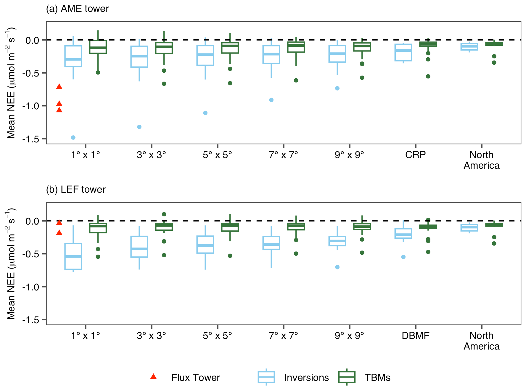
Figure 2Example of consistency in atmospheric inversion and TBM ensembles across spatial scales centered at two grid cells located in the cropland (CRP) and deciduous broadleaf and mixed forest (DBMF) biomes. The AME tower, along with the US-Ne1, US-Ne2, and US-Ne3 flux tower sites, falls within the CRP biome. The LEF tower, along with the US-PFa and US-WCr flux towers, falls within the DBMF biome.
The first two seasonality sub-metrics are the R2 and RMSE between the monthly averaged seasonal cycles of observed CO2 drawdowns or enhancements and of CO2 drawdowns or enhancements resulting from the transported carbon fluxes at each of the four tower locations, for each model. We again use transported signals resulting from spatiotemporal patterns of APAR as a lower benchmark for model performance. A model with an R2 value greater than that of APAR and an RMSE value less than the RMSE value for rescaled APAR is considered to meet the sub-metrics of seasonal variability and magnitude, respectively.
The third sub-metric is the amplitude of the seasonal cycle, which is defined as the difference between the maximum and minimum monthly averaged CO2 concentrations in the average seasonal cycle (Zhao et al., 2016). The model-estimated amplitude of the seasonal cycle is evaluated at each of the four tower locations. We use the amplitude of the seasonal cycle from rescaled APAR as a lower baseline; because the seasonal cycle of APAR is less peaked than that of NEE, the same will be true for the seasonal cycle of the transported signal based on APAR relative to observed CO2 enhancements (Figs. S5, S6). If the amplitude estimated from a model is greater than the amplitude of the transported and rescaled APAR signal, then that model is considered to meet the minimum threshold for the amplitude sub-metric.
The fourth seasonality sub-metric is the timing of peak uptake for the monthly averaged CO2 concentrations, defined as the month when peak uptake occurs. If the predicted peak uptake falls within one month of the observed peak uptake in atmospheric CO2, then the model is considered to pass based on this sub-metric. When applying the overall seasonality metric, a model is kept in the ensemble if it can meet the lower benchmark for at least two of the seasonality sub-metrics at all four tower locations, but the sub-metrics that it meets can vary from tower to tower.
3.1 Model consistency across scales
We find that the full ensemble of TBMs has more consistent carbon flux estimates across all examined spatial scales relative to inversions (Fig. 3a). This is evidenced by TBMs having a smaller standard deviation across the model ensemble for the majority of locations across North America, although there are a few regions where the ensemble of inversions has a smaller standard deviation or where the ensemble with the smaller standard deviation depends on the scale being examined. This result also holds at the biome and continental scale (Fig. 5 “all models”). This result is surprising, because atmospheric inversions are informed by large-scale atmospheric constraints, while TBMs are primarily constrained by process-based understanding derived at fine scales (e.g., plot scale). One would therefore expect that inversions would be more consistent at larger scales than TBMs.
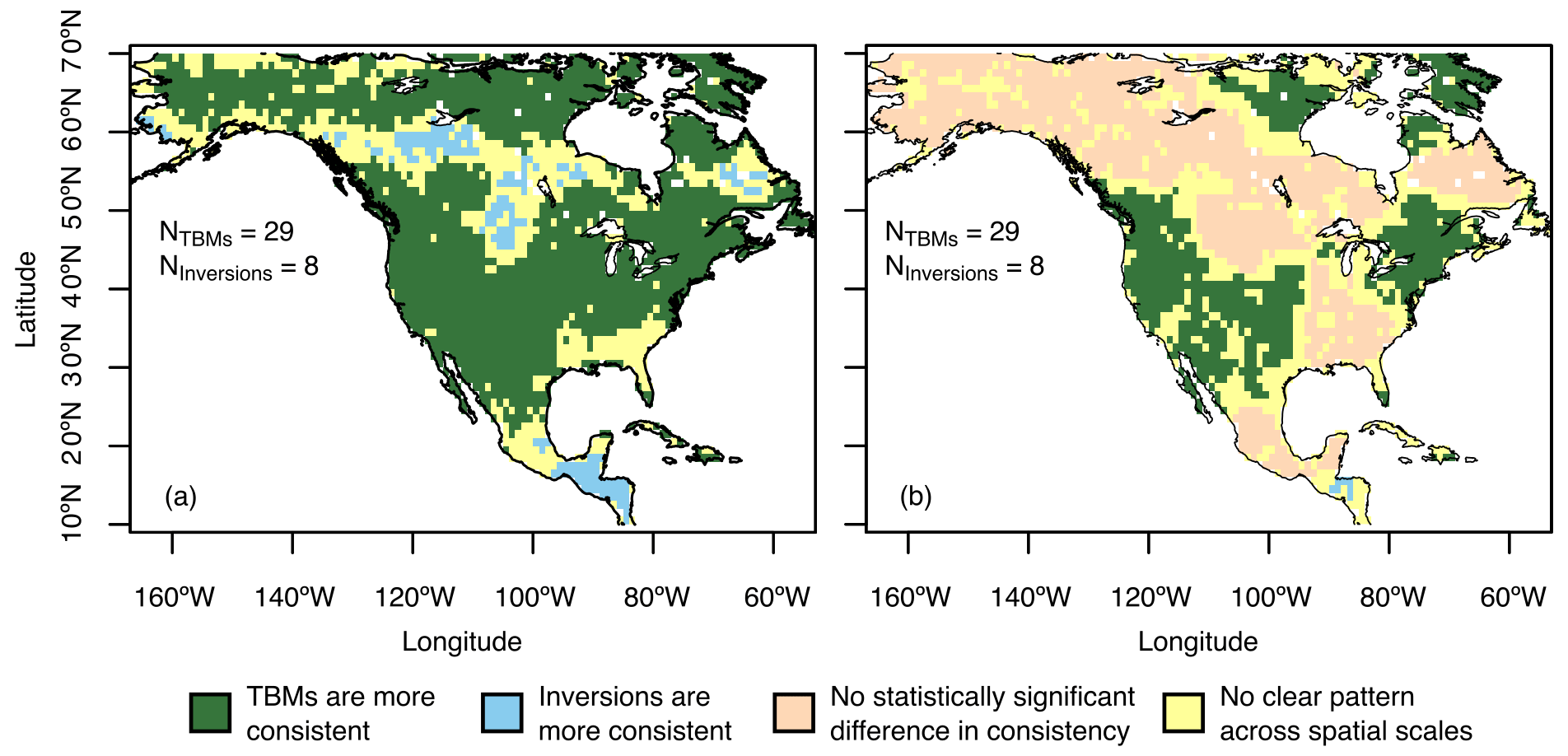
Figure 3Maps showing whether the TBM or the atmospheric inversion ensemble has the more consistent NEE estimates across spatial scales. Maps show where each ensemble has the most consistent estimate (smallest standard deviation) at each of the following scales: , , , , and . Panel (a) shows the most consistent ensemble when the statistical significance of the difference in consistency is not taken into account. Panel (b) shows the result when statistical significance is taken into account. Green regions represent where TBMs have the smaller standard deviation at every examined scale, while blue regions show where inversions are more consistent. Orange regions represent areas where there is no statistically significant difference in consistency at any spatial scale. Yellow regions represent areas where there are inconsistencies across spatial scales. More specifically, in panel (a), yellow regions represent areas where TBMs are more consistent at some scale while inversions are more consistent at other scales, whereas in panel (b) yellow regions represent areas where there is either a mix of statistically significant and not statistically significant differences across spatial scales or where there is a statistically significant difference across all scales, but neither inversion nor TBMs are more consistent across all scales.
However, the difference in the degree of consistency between inversions and TBMs is not statistically significant (p>0.05) for large portions of the continent (Fig. 3b). This is because both ensembles have very high inter-model spread (see examples in Fig. 2), reducing the statistical significance of their differences. These results underscore the importance of statistical significance testing in interpreting model differences.
Earlier studies comparing bottom-up and top-down models have shown varying results in terms of bottom-up versus top-down model consistency for North America. Hayes et al. (2012) reported an average annual NEE estimate for North America of −931 ± 670 TgC yr−1 (mean ± 1 standard deviation) across seven inverse models and −511 ± 729 TgC yr−1 across 12 TBMs for the period of 2000–2006, indicating a slightly higher consistency (lower standard deviation) across inversions at the continental scale. King et al. (2015), on the other hand, reported a mean ± 1 standard deviation annual net land–atmosphere exchange for North America of −890 ± 409 TgC yr−1 across 11 inverse models and −364 ± 120 TgC yr−1 across 10 TBMs for the period 1990–2009, indicating that TBMs were substantially more consistent. The synthesis presented in the State of the Carbon Cycle 2 (SOCCR-2) report further confirmed that the relative consistency among top-down versus bottom-up models varies across studies (Hayes et al., 2018). These earlier studies not only used older versions of model simulations than examined here, but also included far fewer TBMs. At the global scale, the most recent assessment shows that TBMs have a greater model spread (i.e., lower consistency) than do inversions (Friedlingstein et al., 2022). Though these studies are primarily focused on assessing agreement between bottom-up and top-down methods at a single large spatial scale, they demonstrate the difficulty in assessing consistency when ensemble size is limited, and statistical significance is not evaluated. In addition, comparing consistency of bottom-up and top-down models without assessing the statistical significance of observed differences may lead to misleading conclusions. Kondo et al. (2020) found TBMs to have a smaller inter-model spread in regional budget estimates, but the large spread in the seasonality of carbon uptake for TBMs made it difficult to deduce whether bottom-up models are more reliable than top-down models based on consistency alone.
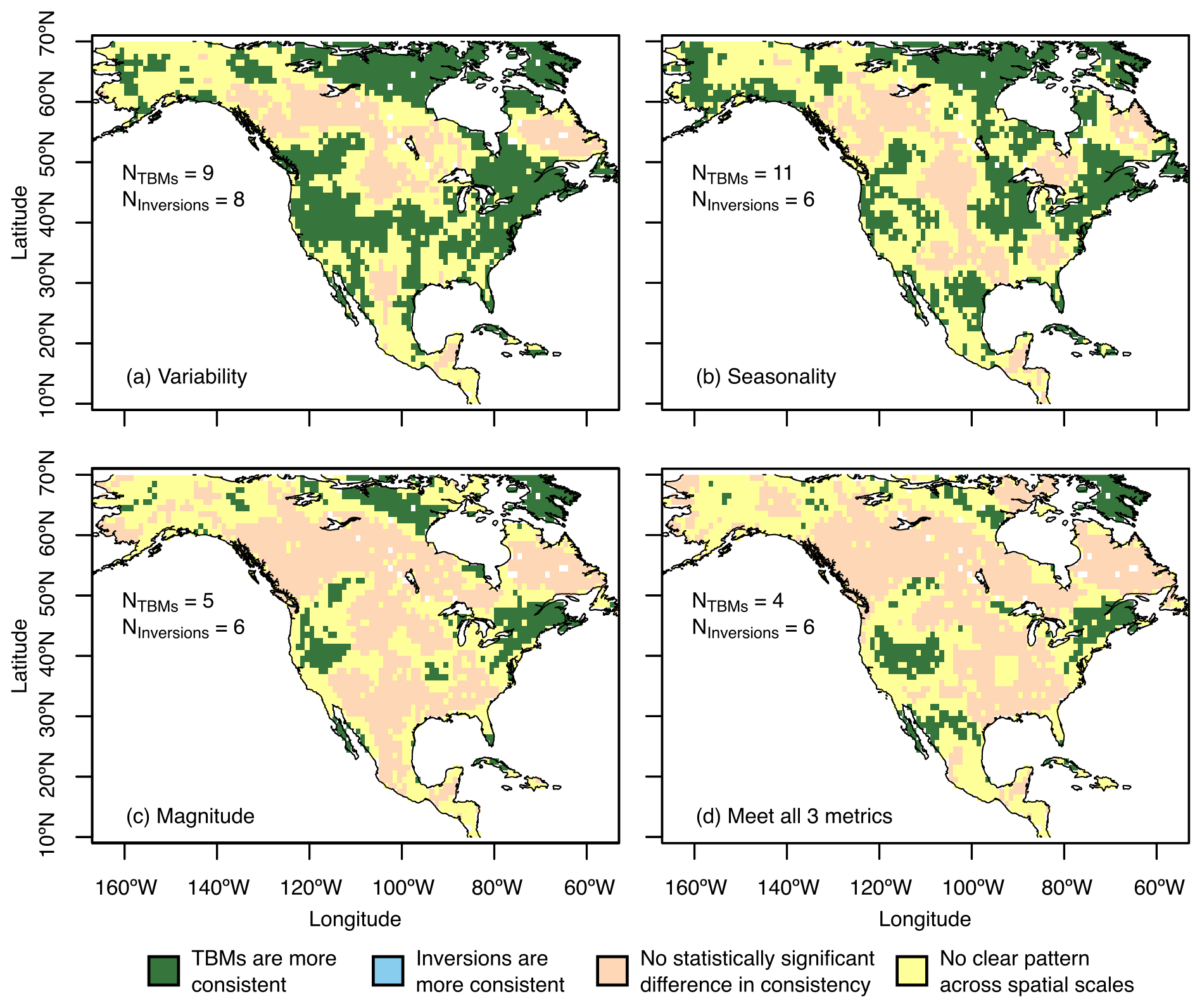
Figure 4Maps showing where the TBM or the atmospheric inversion ensemble has the more consistent NEE estimates across spatial scales when the ensembles are limited to those models that meet (a) variability, (b) seasonality, (c) magnitude, or (d) all three metrics. Colors are as defined in Fig. 3.
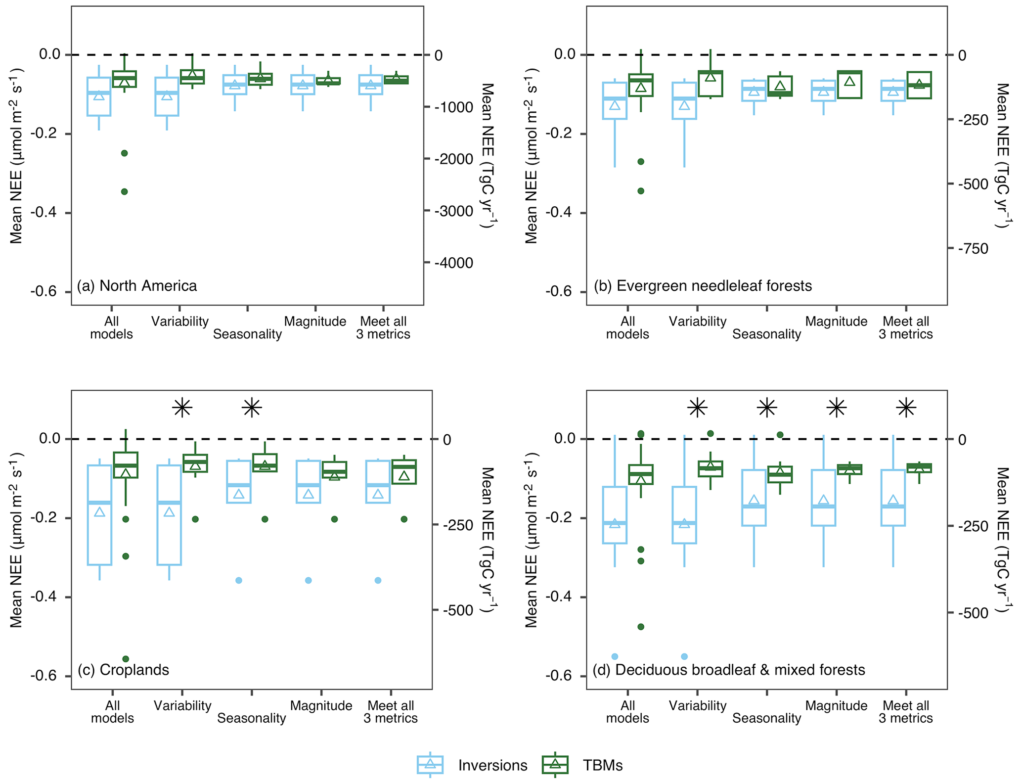
Figure 5Estimated NEE for TBMs and atmospheric inversions for all models within their respective ensembles as well as subsets of the ensembles that meet the variability, seasonality, or magnitude metrics, or that meet all three. Boxplots represent the model-specific average NEE estimates across the models included in each ensemble; triangles represent the across-model mean. Panel (a) shows NEE for North America, while panels (b)–(d) show NEE for specific biomes. Stars represent cases for which there is a statistically significant difference (p<0.05) in the consistency of the TBM versus the inversion ensemble.
While the consistency of model ensembles can be used as one measure of uncertainty in modeling carbon uptake, both bottom-up and top-down methods carry uncertainties that may not be fully captured by ensemble spread alone. For example, the use of satellite data to augment data coverage for atmospheric inversions did not clearly improve consistency in inverse-model-based estimates in a recent intercomparison study (Crowell et al., 2019). Moreover, the differences in the processes incorporated in the various bottom-up models may impact the consistency across the TBM ensemble. We examined how using a simple definition of NEE ( GPP) impacted consistency within the MsTMIP-v2 ensemble and found that estimates from the MsTMIP-v2 ensemble are less consistent across models when using only GPP, Rh, and Ra in the calculation of NEE (Fig. S7). In other words, the models are more consistent when they include other components of NEE, even though those components differ from model to model. This seems to suggest that models may implicitly target a presumed net land sink irrespective of the processes included. This appears to be in line with earlier research that found some TBMs arrive at similar estimates of carbon uptake even though they show large disagreements on the primary driver of increased uptake in recent decades, while other TBMs arrive at dissimilar estimates despite having similar sensitivities (Huntzinger et al., 2017).
3.2 Impact of variability, magnitude, and seasonality on consistency
We evaluate whether greater consistency corresponds to greater accuracy by subsetting the model ensembles using metrics based on the variability, seasonality, and magnitude of atmospheric observations (see Sect. 2.3). Limiting the bottom-up ensemble to only include TBMs that reproduce the variability of atmospheric observations better than APAR reduced the ensemble size from 29 to 9 models. In other words, over two-thirds of TBMs represented the space–time variability of atmospheric CO2 less well than did APAR (Table 1, Fig. S2). Conversely, all inversions performed better than this benchmark (Table 2), which is expected given that the inversions use all or a subset of the same observations in estimating fluxes. Sub-selecting models that could represent aspects of the seasonality of atmospheric observations reduced the ensemble of TBMs from 29 to 11 and the ensemble of inversions from 8 to 6. Limiting the ensembles to models that could represent the magnitude of observed atmospheric CO2 signals reduced the ensemble of TBMs from 29 to 5, while the ensemble of inversions was reduced from 8 to 6. Only four TBMs (and six inversions) remained when all three metrics were applied. For the four TBMs that are in both the MsTMIP-v2 and TRENDY-v9 ensembles, we retained the TRENDY-v9 simulations as described in Sect. 2.1.1. Had we included the three MsTMIP-v2 simulations, however, none of them met any of the three metrics and they therefore would have been excluded from the subsets meeting the variability, seasonality, and magnitude metrics.
The large reduction in the ensemble size when even basic benchmarks related to observed atmospheric CO2 signals are applied (i.e., filtering based on a minimum accuracy threshold) indicates that ensemble spread (i.e., consistency) is unlikely to be a good indicator of actual uncertainty in our understanding of North American carbon balance. An example of consistency not necessarily capturing uncertainty is shown in Fig. 2 at the scale where TBMs and inversions show better agreement with eddy covariance flux tower observations in the deciduous broadleaf and mixed forest biome (Fig. 2b) than in the cropland biome (Fig. 2a) despite having similar model consistency in both biomes. It is unclear whether the models and observations disagree in the cropland biome due to sub-grid scale heterogeneity (Melton and Arora, 2014) versus inaccuracies in the models (Schuh et al., 2014; Guanter et al., 2014; Sun et al., 2021), but this comparison nevertheless illustrates how consistency may not capture the full extent of uncertainty in model simulations.
Fang et al. (2014) also noted that atmospheric observations can be used to evaluate flux patterns from TBMs in terms of models' ability to explain atmospheric observations. Using a similar approach here we see that differentiating between models that reproduce basic features of atmospheric CO2 signals leads to a shift from TBMs having the smaller ensemble standard deviation across scales to there being no statistically significant difference between the ensemble standard deviations of TBMs and inversions across most of the continent. This is particularly true when models are selected based on consistency with all three metrics.
Applying the variability, magnitude, and seasonality metrics reduces the areas in North America for which TBMs have a statistically significantly greater consistency than do inversions (Fig. 4). Once all three metrics are applied, very few areas remain where TBMs have a higher consistency across all scales. This result is enlightening, because it indicates that once basic aspects of atmospheric observational constraints are taken into account, apparent differences in consistency between approaches disappear. The large reduction in the TBM ensemble size is part of the reason for this change, so this result must be interpreted with caution. In other words, this result is less a product of the consistency of remaining inversions increasing and more a product of the statistical significance of differences in consistency being reduced due to the reduction in the sample size. This filtering exercise also indicates that, although the ensemble of inversions examined here has lower consistency, it may actually exhibit higher accuracy as evidenced by the smaller reduction in ensemble size and higher number of models that meet all three criteria.
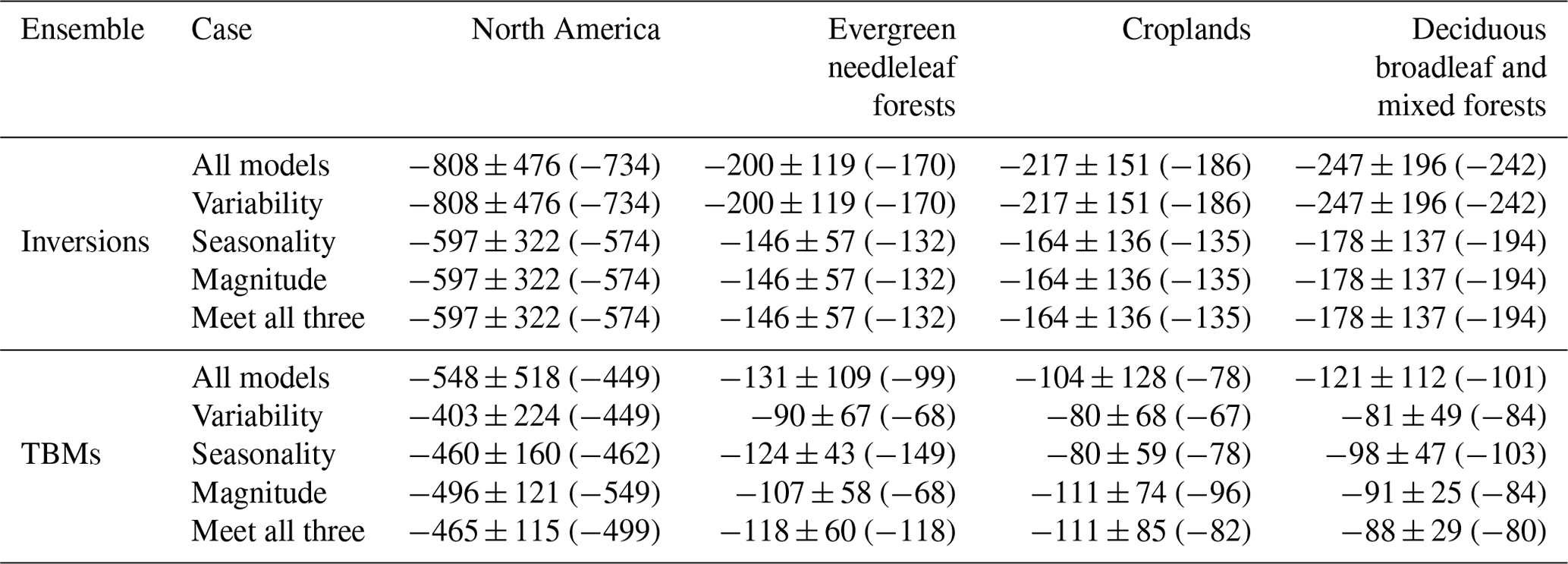
Table 2Impact of filtering ensembles based on key metrics derived from observational constraints. The mean ± standard deviation (median) fluxes (in units of TgC yr−1) for inversions and TBMs when metrics are applied to North America and biomes with the largest data constraint across 2007–2010.
3.3 Implications for understanding of North American carbon balance
3.3.1 Impact on model consistency
The impact of applying accuracy metrics to the ensembles offers a glimpse into the true North American carbon sink. While this approach did increase model consistency for TBMs, it did not impact model consistency for atmospheric inversions. The lack of increase in the consistency of inversions once accuracy metrics are applied indicates that there is a wide range of overall flux patterns and magnitudes that are consistent with large-scale atmospheric constraints. It is interesting, therefore, that model consistency among TBMs does increase substantially when accuracy metrics are applied (Fig. 5), although again this has to be interpreted with caution given the small number of remaining models. This contrast implies that, once accuracy metrics are applied, remaining TBMs all reproduce observed features of atmospheric observations using similar flux patterns, while remaining inversions reproduce observed features of atmospheric observations using a wider range of fluxes. The large spread of inversions that are also consistent with the same atmospheric constraints indicates that consistency across model ensembles is likely a poor indicator of overall uncertainty. This suggests that decreases in model spread do not necessarily indicate increases in model accuracy, as has also been suggested in previous studies (Annan and Hargreaves, 2010; Knutti et al., 2010; Kondo et al., 2020; Lovenduski and Bonan, 2017). Because TBMs were already informed by process-based understanding, subsetting the ensemble to those TBMs that are also consistent with broad features of atmospheric CO2 observations may lead to the “best of both worlds”. The high consistency of the remaining (albeit small number of) TBMs is a sign that these models are more likely to capture the true North American carbon sink.
3.3.2 Impact on model agreement
Most promisingly, not only does the difference in consistency between top-down and bottom-up models decrease when ensembles are filtered based on key metrics derived from observational constraints, but the agreement between top-down and bottom-up models improves dramatically as well (Fig. 5a). Indeed, once all three metrics are applied, both the mean and the median across the remaining TBMs are very close to the mean and the median across the remaining inversions. In other words, filtering leads to better agreement between top-down and bottom-up estimates of North American carbon balance, a goal that has proven elusive up to now. The mean (median) North American fluxes across 2007–2010, when all three criteria are applied, is −465 TgC yr−1 (−499 TgC yr−1) for the TBMs and −597 TgC yr−1 (−574 TgC yr−1) for the inversions (Table 2).
Agreement for the three biomes that are best-constrained by atmospheric observations is also improved (Fig. 5b, c, d) although to a lesser extent. These biomes are evergreen needleleaf forests, croplands, and deciduous broadleaf and mixed forests biomes, based on an analysis by Sun et al. (2023) that showed these biomes to have the greatest sensitivity of atmospheric observations to fluxes (2023). When the seasonality metric is recalculated using eight towers selected from the sensitivity analysis (see Sect. 2.3), there are minimal changes to agreement between bottom-up and top-down estimates. The deciduous broadleaf and mixed forests, which is the biome with the lowest observational constraint of the three biomes, showed decreased agreement suggesting that using towers with high temporal data availability, rather than more towers, is important for capturing seasonality. The mean (median) uptake for evergreen needleleaf forests when all three metrics are applied is −118 TgC yr−1 (−118 TgC yr−1) for the TBMs and −146 TgC yr−1 (−132 TgC yr−1) for the inversions (Table 2). For croplands, the mean (median) is −111 TgC yr−1 (−82 TgC yr−1) for the TBMs and −164 TgC yr−1 (−135 TgC yr−1) for the inversions (Table 2). The mean (median) for deciduous broadleaf and mixed forests is −88 TgC yr−1 (−80 TgC yr−1) for the TBMs and −178 TgC yr−1 (−194 TgC yr−1) for the inversions (Table 2).
Lower improvement in the agreement between TBMs and inversions at the biome scale relative to the continental scale may have resulted from disagreement on where major sinks in North America lie. However, to understand why models disagree, it is necessary to understand what gives rise to differences. For example, deciduous broadleaf and mixed forests were found to account for the majority of the interannual variability in NEE for North America when using a top-down approach, but TBMs disagreed on whether forested or non-forested biomes contribute most strongly to interannual variability and what the primary environmental drivers of this variability are (Shiga et al., 2018b). TBMs have also been shown to have greater interannual variability in western temperate North America than in eastern temperate North America, albeit with substantial model spread (Byrne et al., 2020). A recent study found that TBMs that did well at reproducing observed CO2 variability exhibited substantially stronger growing-season carbon uptake in croplands relative to other models (Sun et al., 2021). These studies highlight that there is still uncertainty about the geographic distribution, interannual variability, and climatic drivers of North American carbon uptake. This likely plays a role in the reduced agreement at the biome scale relative to the continental scale observed here.
3.3.3 Sensitivity analyses and study limitations
One potential reason for the lack of convergence between bottom-up and top-down approaches is the limited number of towers used for the seasonality metrics. These towers are primarily located in the midcontinent (Fig. 1), although observations from towers are also influenced by fluxes in other regions (see, e.g., Extended Data Fig. 2 in Sun et al., 2023). To test this this hypothesis, we conducted a sensitivity analysis to explore the impact of including four additional towers (see Sect. 2.3). We found that including more towers in other parts of North America did not change our primary findings. Specifically, we found that 11 models perform well based on the seasonality metric irrespective of which subset of towers is used (i.e., original four towers, additional four towers, or all eight towers), while six and four additional models also meet the metric when the original and additional sets of four towers are used, respectively. Though modifying the towers used impacts the consistency of ensembles based on the seasonality metric alone, the impact on the consistency and agreement of models that meet all three metrics is minimal (Fig. S8).
While increased data availability in biomes that are not well sampled would allow for a more robust evaluation of models' ability to capture key aspects of seasonality, several studies have found that even in areas with high data availability there is still noticeable disagreement between inversions (Bastos et al., 2020; Kondo et al., 2020). This indicates that model-specific issues may be more important than data availability in explaining discrepancies between bottom-up and top-down estimates. In the context of inverse modeling, the choice of fossil fuel inventory and transport model have been identified as significant sources of uncertainties, though there is not a clear consensus as to what the primary source of uncertainty is (Bastos et al., 2020; Gaubert et al., 2019; Peylin et al., 2011; Schuh et al., 2019). For TBMs, noteworthy uncertainties stem from how (and whether) models represent key processes such as land use change, wood and crop harvesting, fire, and vegetation dynamics (Ahlström et al., 2015; Bastos et al., 2020; Hardouin et al., 2022; Tharammal et al., 2019).
Several studies also highlight lateral fluxes as a significant source of CO2 emissions, yet many TBMs do not account for them (Drake et al., 2018; Kondo et al., 2020; Raymond et al., 2013). To test the possible impact of lateral fluxes on our analysis, we examined the effect of including lateral fluxes in bottom-up estimates on the agreement between bottom-up and top-down methods. To do so, we added gridded lateral fluxes of river export, crop trade, and wood trade to TBMs to make them more comparable with fluxes seen by inversions. We used two different estimates of river export from Byrne et al. (2023). The first is the gridded product, which incorporates results from the Global NEWS model (Byrne et al., 2022). The second is the same gridded product rescaled, so total river export equals the country total river exports reported in Byrne et al. (2023), which is the mean of two models estimates (Global NEWS and DLEM). The differences in these two river export estimates highlight some of the uncertainties associated with estimating lateral fluxes (Byrne et al., 2023; Drake et al., 2018). We find that at the North American scale, incorporating lateral fluxes improved agreement between bottom-up and top-down models somewhat, but the change was not sufficient to explain discrepancies for the best-constrained biomes (Fig. S9). In the deciduous broadleaf and mixed forests and cropland biomes, lateral fluxes only partially explain discrepancies and applying the seasonality, variability, and magnitude metrics still improved agreement between bottom-up and top-down estimates (Fig. S9c–d). This contrasts with the evergreen and needle leaf forest biome where the inclusion of lateral fluxes led to better agreement between inversions and TBMs for the subset with all models included but ultimately exacerbated differences once models that meet all three criteria were selected (Fig. S9b). This aligns with the findings of Kondo et al. (2020) that accounting for lateral fluxes and using a standardized net CO2 flux definition was not sufficient to explain discrepancies between inversions and TBMs at regional scales.
Next we explored whether agreement between top-down and bottom-up estimates was improved when a more consistent definition of NEE was applied to TBMs. To do so, we examined how using a simple definition of NEE ( GPP) impacted agreement between MsTMIP-v2 models and inversions; we found that agreement with inversions improved slightly (Fig. S7). Of the MsTMIP-v2 models we looked at, only four included both disturbance and product fluxes in their definition of NEE (CLM4, CLM4VIC, TEM6, VEGAS2.1), and how well these models agree with inversions varies by biome (Fig. S7). Bastos et al. (2020) found that models, irrespective of their inclusion of fire dynamics, exhibited similar performance, which could be attributed to heightened sensitivity of decomposition to temperature in models without fire. Moreover, Huntzinger et al. (2017) found TBMs can yield similar estimates despite diverging on their primary drivers. We therefore found that it is unlikely that varying NEE definitions provide a comprehensive explanation for the observed disparities.
There are additional sources of uncertainty that the sensitivity analyses described here cannot address. For example, the non-uniform spatial distribution of observation data throughout the domain limits the biomes that can be examined. Additional observations, particularly in regions that are not well sampled, would allow for additional analyses and would further increase the robustness of the continental-scale results. Leveraging larger ensembles of TBMs and inversions and incorporating an assessment of the impact of transport model choice would also allow for additional insight into the robustness of our findings. Though we showed that TBM estimates of North American carbon sink were actually more consistent when varying NEE definitions were used and that discrepancies between bottom-up and top-down models cannot be fully resolved by the incorporation of lateral fluxes, improved standardization across TBMs in terms of represented processes would allow for a more accurate comparison with inversions. Finally, it is important to recognize that better performance under present climate conditions does not necessarily translate to better model performance under future conditions.
Comparing estimates from bottom-up and top-down methods across spatial scales and evaluating estimates in light of atmospheric CO2 observations is useful for exploring persistent differences between these approaches. We show that the difference in consistency between bottom-up and top-down ensembles is not statistically significant for large regions of North America because of large variability within both ensembles, highlighting the importance of significance testing in interpreting model differences. We also find that ensemble spread is unlikely to be a good indicator of overall uncertainty in the North American carbon balance. This is because when the same benchmarks based on observed atmospheric CO2 signals are applied to both ensembles, inversions use a wider range of fluxes than TBMs to reproduce observed atmospheric observation features. Encouragingly, once models are sub-selected based on their ability to reproduce basic aspects of observed atmospheric CO2 variability, seasonality, and magnitude, bottom-up and top-down estimates of North American carbon balance agree at the continental scale and for large biomes therein. Notably, these findings remained robust after several sensitivity analyses were performed. The convergence in flux estimates between top-down and bottom-up approaches demonstrates the usefulness of filtering models based on their agreement with even basic features of large-scale observational constraints for assessing our understanding of carbon budgets. This finding is encouraging because it presents a promising path towards both improving model consistency and reducing uncertainties. Thus, continued efforts to reduce uncertainties should focus on improving consistency at scales finer than large continental domains and leveraging top-down observational constraints to refine understanding of the North American carbon balance.
All data used are publicly available and the sources are provided in Sect. 2 and Tables 1 and S1.
The supplement related to this article is available online at: https://doi.org/10.5194/bg-21-869-2024-supplement.
AMM and KTF designed the study. WS, YPS, and KTF collected the data and prepared them for analysis. KTF prepared figures and wrote the manuscript with contributions from all authors.
The contact author has declared that none of the authors has any competing interests.
Publisher’s note: Copernicus Publications remains neutral with regard to jurisdictional claims made in the text, published maps, institutional affiliations, or any other geographical representation in this paper. While Copernicus Publications makes every effort to include appropriate place names, the final responsibility lies with the authors.
The authors thank Trevor Keenan and Xiangzhong Luo for processing and providing the MODIS FPAR data. We acknowledge the NCEP North American Regional Reanalysis data provided by the NOAA Physical Sciences Laboratory, Boulder, Colorado, USA (obtained from https://psl.noaa.gov/, last access: 12 July 2023). We thank all modelers and investigators who contributed to the Multi-scale synthesis and Terrestrial Model Intercomparison Project (MsTMIP; http://nacp.ornl.gov/MsTMIP. shtml, last access: 12 July 2023). Funding for the Multi-scale synthesis and Terrestrial Model Intercomparison Project activity was provided through NASA ROSES grant no. NNX10AG01A. Data management support for preparing, documenting, and distributing model driver and output data was performed by the Modeling and Synthesis Thematic Data Center at Oak Ridge National Laboratory (ORNL; https://nacp.ornl.gov, last access: 12 July 2023), with funding through NASA ROSES grant no. NNH10AN681. Finalized MsTMIP data products are archived at the ORNL DAAC (https://daac.ornl.gov, last access: 12 July 2023). The authors thank Stephen Sitch, Pierre Friedlingstein, and all modelers of the Trends in Net Land-Atmosphere Exchange project (TRENDY; https://blogs.exeter.ac.uk/trendy/, last access: 12 July 2023). We thank the following individuals for collecting and providing the atmospheric CO2 data from the following sites: Arlyn Andrews for AMT, BAO, LEF, WBI, and WKT; Arlyn Andrews and Marc L. Fischer for WGC; Arlyn Andrews and Matt J. Parker for SCT; Arlyn Andrews and Stephan De Wekker for SNP; Sebastien Biraud and Margaret Torn for SGP; Tim Griffis for KCMP; Beverly Law, Andres Schmidt, and the TERRA-PNW group for data from the five Oregon sites OFR, OMP, OMT, ONG, and OYQ; Natasha Miles, Scott Richardson, and Ken Davis for AAC, ACR, ACV, AME, AOZ, FPK, RCE, RGV, RKW, RMM, and RRL; Britton Stephens and the Regional Atmospheric Continuous CO2 Network in the Rocky Mountains (RACCOON) for HDP, NWR, RBA, and SPL; Colm Sweeney for MVY; Kirk Thoning and Pieter Tans for BRW; Steven Wofsy and William Munger for HFM; Doug Worthy for BCK, BRA, CDL, CHM, EGB, ESP, EST, ETL, FSD, LLB, and WSA. Measurements at WGC were partially supported by grants from the California Energy Commission (CEC) Public Interest Environmental Research Program to the Lawrence Berkeley National Laboratory, which operates under US Department of Energy under contract no. DE-AC02-05CH11231. The authors thank the Atmospheric and Environmental Research, Inc. (AER) – particularly, Thomas Nehrkorn, John Henderson, and Janusz Eluszkiewicz – for conducting WRF-STILT simulations and providing transport footprints. We thank the CarbonTracker-Lagrange project team for proving the WRF-STILT transport footprints. The authors thank Kevin Gurney for FFDAS v2 data. We thank the CarbonTracker team for the CarbonTracker CT2019B results provided by the NOAA Global Monitoring Laboratory, Boulder, Colorado, USA (http://carbontracker.noaa.gov, last access: 12 July 2023). We thank the CarbonTracker-Lagrange team for terrestrial CO2 fluxes data. We thank the CarbonTracker Europe team for the CarbonTracker Europe results provided by Wageningen University in collaboration with the ObsPack partners (http://www.carbontracker.eu, last access: 12 July 2023). We thank the Copernicus Atmosphere Monitoring Service (CAMS) team for the CAMS inversion results generated using Copernicus Atmosphere Monitoring Service Information (2020). Neither the European Commission nor ECMWF is responsible for any use that may be made of the information it contains. We thank Christian Rödenbeck for CarboScope-sEXTocNEET data (retrieved from http://www.bgc-jena.mpg.de/CarboScope/?ID=sEXTocNEET_v4.3, last access: 12 July 2023). We thank the MIROC-ACTM team for the MIROC-ACTM inversions results that are provided by JAMSTEC (ArCS-II grant no. JPMXD1420318865, and ERTDF SII-8 grant no. JPMEERF21S20800).
The computations presented here were conducted through Carnegie's partnership in the Resnick High Performance Computing Center, a facility supported by Resnick Sustainability Institute at the California Institute of Technology.
Wu Sun and Kelsey T. Foster receive funding support by NASA through the Carbon Monitoring System (grant no. 80NSSC18K0165) and the Terrestrial Ecology programs (grant no. 80NSSC22K1253), with additional support from the Carnegie Institution for Science’s endowment fund. Jiafu Mao was supported by the Terrestrial Ecosystem Science Scientific Focus Area (TES SFA) project funded by the US Department of Energy, Office of Science, Office of Biological and Environmental Research. Oak Ridge National Laboratory is supported by the Office of Science of the US Department of Energy under contract no. DEAC05-00OR22725.
This paper was edited by Paul Stoy and reviewed by Guillermo Murray-Tortarolo and Xinyuan Wei.
Ahlström, A., Xia, J., Arneth, A., Luo, Y., and Smith, B.: Importance of vegetation dynamics for future terrestrial carbon cycling, Environ. Res. Lett., 10, 054019, https://doi.org/10.1088/1748-9326/10/5/054019, 2015.
Andrews, A. E., Kofler, J. D., Trudeau, M. E., Williams, J. C., Neff, D. H., Masarie, K. A., Chao, D. Y., Kitzis, D. R., Novelli, P. C., Zhao, C. L., Dlugokencky, E. J., Lang, P. M., Crotwell, M. J., Fischer, M. L., Parker, M. J., Lee, J. T., Baumann, D. D., Desai, A. R., Stanier, C. O., De Wekker, S. F. J., Wolfe, D. E., Munger, J. W., and Tans, P. P.: CO2, CO, and CH4 measurements from tall towers in the NOAA Earth System Research Laboratory's Global Greenhouse Gas Reference Network: instrumentation, uncertainty analysis, and recommendations for future high-accuracy greenhouse gas monitoring efforts, Atmos. Meas. Tech., 7, 647–687, https://doi.org/10.5194/amt-7-647-2014, 2014.
Annan, J. D. and Hargreaves, J. C.: Reliability of the CMIP3 ensemble, Geophys. Res. Lett., 37, L02703, https://doi.org/10.1029/2009GL041994, 2010.
Asefi-Najafabady, S., Rayner, P. J., Gurney, K. R., McRobert, A., Song, Y., Coltin, K., Huang, J., Elvidge, C., and Baugh, K.: A multiyear, global gridded fossil fuel CO2 emission data product: Evaluation and analysis of results, J. Geophys. Res.-Atmos., 119, 10213–10231, https://doi.org/10.1002/2013JD021296, 2014.
Baker, D. F., Law, R. M., Gurney, K. R., Rayner, P., Peylin, P., Denning, A. S., Bousquet, P., Bruhwiler, L., Chen, Y.-H., Ciais, P., Fung, I. Y., Heimann, M., John, J., Maki, T., Maksyutov, S., Masarie, K., Prather, M., Pak, B., Taguchi, S., and Zhu, Z.: TransCom 3 inversion intercomparison: Impact of transport model errors on the interannual variability of regional CO2 fluxes, 1988–2003, Global Biogeochem. Cy., 20, 1, https://doi.org/10.1029/2004GB002439, 2006.
Baker, I. T., Prihodko, L., Denning, A. S., Goulden, M., Miller, S., and da Rocha, H. R.: Seasonal drought stress in the Amazon: Reconciling models and observations, J. Geophys. Res.-Biogeo., 113, G00B01, https://doi.org/10.1029/2007JG000644, 2008.
Baldocchi, D.: “Breathing” of the terrestrial biosphere: lessons learned from a global network of carbon dioxide flux measurement systems, Aust. J. Bot., 56, 1–26, https://doi.org/10.1071/BT07151, 2008.
Bastos, A., O'Sullivan, M., Ciais, P., Makowski, D., Sitch, S., Friedlingstein, P., Chevallier, F., Rödenbeck, C., Pongratz, J., Luijkx, I. T., Patra, P. K., Peylin, P., Canadell, J. G., Lauerwald, R., Li, W., Smith, N. E., Peters, W., Goll, D. S., Jain, A. K., Kato, E., Lienert, S., Lombardozzi, D. L., Haverd, V., Nabel, J. E. M. S., Poulter, B., Tian, H., Walker, A. P., and Zaehle, S.: Sources of Uncertainty in Regional and Global Terrestrial CO2 Exchange Estimates, Global Biogeochem. Cy., 34, e2019GB006393, https://doi.org/10.1029/2019GB006393, 2020.
Bergamaschi, P., Frankenberg, C., Meirink, J. F., Krol, M., Dentener, F., Wagner, T., Platt, U., Kaplan, J. O., Körner, S., Heimann, M., Dlugokencky, E. J., and Goede, A.: Satellite chartography of atmospheric methane from SCIAMACHY on board ENVISAT: 2. Evaluation based on inverse model simulations, J. Geophys. Res.-Atmos., 112, D02304, https://doi.org/10.1029/2006JD007268, 2007.
Bergamaschi, P., Frankenberg, C., Meirink, J. F., Krol, M., Villani, M. G., Houweling, S., Dentener, F., Dlugokencky, E. J., Miller, J. B., Gatti, L. V., Engel, A., and Levin, I.: Inverse modeling of global and regional CH4 emissions using SCIAMACHY satellite retrievals, J. Geophys. Res.-Atmos., 114, D22301, https://doi.org/10.1029/2009JD012287, 2009.
Bonan, G. B. and Levis, S.: Quantifying carbon-nitrogen feedbacks in the Community Land Model (CLM4), Geophys. Res. Lett., 37, L07401, https://doi.org/10.1029/2010GL042430, 2010.
Bonan, G. B., Lombardozzi, D. L., Wieder, W. R., Oleson, K. W., Lawrence, D. M., Hoffman, F. M., and Collier, N.: Model Structure and Climate Data Uncertainty in Historical Simulations of the Terrestrial Carbon Cycle (1850–2014), Global Biogeochem. Cy., 33, 1310–1326, https://doi.org/10.1029/2019GB006175, 2019.
Brovkin, V. and Goll, D.: Land unlikely to become large carbon source, Nat. Geosci., 8, 893–893, https://doi.org/10.1038/ngeo2598, 2015.
Burke, E. J., Jones, C. D., and Koven, C. D.: Estimating the Permafrost-Carbon Climate Response in the CMIP5 Climate Models Using a Simplified Approach, J. Clim., 26, 4897–4909, https://doi.org/10.1175/JCLI-D-12-00550.1, 2013.
Byrne, B., Liu, J., Bloom, A. A., Bowman, K. W., Butterfield, Z., Joiner, J., Keenan, T. F., Keppel-Aleks, G., Parazoo, N. C., and Yin, Y.: Contrasting Regional Carbon Cycle Responses to Seasonal Climate Anomalies Across the East-West Divide of Temperate North America, Global Biogeochem. Cy., 34, e2020GB006598, https://doi.org/10.1029/2020GB006598, 2020.
Byrne, B., Baker, D. F., Basu, S., Bertolacci, M., Bowman, K. W., Carroll, D., Chatterjee, A., Chevallier, F., Ciais, P., Cressie, N., Crisp, D., Crowell, S., Deng, F., Deng, Z., Deutscher, N. M., Dubey, M. K., Feng, S., García, O. E., Herkommer, B., Hu, L., Jacobson, A. R., Janardanan, R., Jeong, S., Johnson, M. S., Jones, D. B. A., Kivi, R., Liu, J., Liu, Z., Maksyutov, S., Miller, J. B., Miller, S. M., Morino, I., Notholt, J., Oda, T., O'Dell, C. W., Oh, Y.-S., Ohyama, H., Patra, P. K., Peiro, H., Petri, C., Philip, S., Pollard, D. F., Poulter, B., Remaud, M., Schuh, A., Sha, M. K., Shiomi, K., Strong, K., Sweeney, C., Té, Y., Tian, H., Velazco, V. A., Vrekoussis, M., Warneke, T., Worden, J. R., Wunch, D., Yao, Y., Yun, J., Zammit-Mangion, A., and Zeng, N.: Pilot top-down CO2 Budget constrained by the v10 OCO-2 MIP Version 1, Committee on Earth Observing Satellites, https://doi.org/10.48588/npf6-sw92, Version 1.0, 2022
Byrne, B., Baker, D. F., Basu, S., Bertolacci, M., Bowman, K. W., Carroll, D., Chatterjee, A., Chevallier, F., Ciais, P., Cressie, N., Crisp, D., Crowell, S., Deng, F., Deng, Z., Deutscher, N. M., Dubey, M. K., Feng, S., García, O. E., Griffith, D. W. T., Herkommer, B., Hu, L., Jacobson, A. R., Janardanan, R., Jeong, S., Johnson, M. S., Jones, D. B. A., Kivi, R., Liu, J., Liu, Z., Maksyutov, S., Miller, J. B., Miller, S. M., Morino, I., Notholt, J., Oda, T., O'Dell, C. W., Oh, Y.-S., Ohyama, H., Patra, P. K., Peiro, H., Petri, C., Philip, S., Pollard, D. F., Poulter, B., Remaud, M., Schuh, A., Sha, M. K., Shiomi, K., Strong, K., Sweeney, C., Té, Y., Tian, H., Velazco, V. A., Vrekoussis, M., Warneke, T., Worden, J. R., Wunch, D., Yao, Y., Yun, J., Zammit-Mangion, A., and Zeng, N.: National CO2 budgets (2015–2020) inferred from atmospheric CO2 observations in support of the global stocktake, Earth Syst. Sci. Data, 15, 963–1004, https://doi.org/10.5194/essd-15-963-2023, 2023.
Canadell, J. G., Ciais, P., Gurney, K., Quéré, C. L., Piao, S., Raupach, M. R., and Sabine, C. L.: An International Effort to Quantify Regional Carbon Fluxes, Eos, Transactions American Geophysical Union, 92, 81–82, https://doi.org/10.1029/2011EO100001, 2011.
Chandra, N., Patra, P. K., Niwa, Y., Ito, A., Iida, Y., Goto, D., Morimoto, S., Kondo, M., Takigawa, M., Hajima, T., and Watanabe, M.: Estimated regional CO2 flux and uncertainty based on an ensemble of atmospheric CO2 inversions, Atmos. Chem. Phys., 22, 9215–9243, https://doi.org/10.5194/acp-22-9215-2022, 2022.
Chevallier, F., Ciais, P., Conway, T. J., Aalto, T., Anderson, B. E., Bousquet, P., Brunke, E. G., Ciattaglia, L., Esaki, Y., Fröhlich, M., Gomez, A., Gomez-Pelaez, A. J., Haszpra, L., Krummel, P. B., Langenfelds, R. L., Leuenberger, M., Machida, T., Maignan, F., Matsueda, H., Morguí, J. A., Mukai, H., Nakazawa, T., Peylin, P., Ramonet, M., Rivier, L., Sawa, Y., Schmidt, M., Steele, L. P., Vay, S. A., Vermeulen, A. T., Wofsy, S., and Worthy, D.: CO2 surface fluxes at grid point scale estimated from a global 21 year reanalysis of atmospheric measurements, J. Geophys. Res.-Atmos., 115, D21307, https://doi.org/10.1029/2010JD013887, 2010.
Chevallier, F., Palmer, P. I., Feng, L., Boesch, H., O'Dell, C. W., and Bousquet, P.: Toward robust and consistent regional CO2 flux estimates from in situ and spaceborne measurements of atmospheric CO2, Geophys. Res. Lett., 41, 1065–1070, https://doi.org/10.1002/2013GL058772, 2014.
Ciais, P., Bastos, A., Chevallier, F., Lauerwald, R., Poulter, B., Canadell, J. G., Hugelius, G., Jackson, R. B., Jain, A., Jones, M., Kondo, M., Luijkx, I. T., Patra, P. K., Peters, W., Pongratz, J., Petrescu, A. M. R., Piao, S., Qiu, C., Von Randow, C., Regnier, P., Saunois, M., Scholes, R., Shvidenko, A., Tian, H., Yang, H., Wang, X., and Zheng, B.: Definitions and methods to estimate regional land carbon fluxes for the second phase of the REgional Carbon Cycle Assessment and Processes Project (RECCAP-2), Geosci. Model Dev., 15, 1289–1316, https://doi.org/10.5194/gmd-15-1289-2022, 2022.
Ciais, P., Sabine, C., Bala, G., Bopp, L., Brovkin, V., Canadell, J., Chhabra, A., DeFries, R., Galloway, J., Heimann, M., Jones, C., Le Quéré, C., Myneni, R. B., Piao S., and Thornton, P.: Carbon and other biogeochemical cycles, in: Climate change 2013: The physical science basis, contribution of working group I to the fifth assessment report of the Intergovernmental Panel on Climate Change, edited by: Stocker, T. F., Qin, D., Plattner, G.-K., Tignor, M., Allen, S. K., Boschung, J., and Midgley, P. M., 465–570, Cambridge, UK, Cambridge University Press, 2013.
Ciais, P., Canadell, J. G., Luyssaert, S., Chevallier, F., Shvidenko, A., Poussi, Z., Jonas, M., Peylin, P., King, A. W., Schulze, E.-D., Piao, S., Rödenbeck, C., Peters, W., and Bréon, F.-M.: Can we reconcile atmospheric estimates of the Northern terrestrial carbon sink with land-based accounting?, Curr. Opin. Environ. Sustain., 2, 225–230, https://doi.org/10.1016/j.cosust.2010.06.008, 2010.
Ciais, P., Rayner, P., Chevallier, F., Bousquet, P., Logan, M., Peylin, P., and Ramonet, M.: Atmospheric inversions for estimating CO2 fluxes: methods and perspectives, in: Greenhouse Gas Inventories: Dealing With Uncertainty, edited by: Jonas, M., Nahorski, Z., Nilsson, S., and Whiter, T., Springer Netherlands, Dordrecht, 69–92, https://doi.org/10.1007/978-94-007-1670-4_6, 2011.
Clark, D. B., Mercado, L. M., Sitch, S., Jones, C. D., Gedney, N., Best, M. J., Pryor, M., Rooney, G. G., Essery, R. L. H., Blyth, E., Boucher, O., Harding, R. J., Huntingford, C., and Cox, P. M.: The Joint UK Land Environment Simulator (JULES), model description – Part 2: Carbon fluxes and vegetation dynamics, Geosci. Model Dev., 4, 701–722, https://doi.org/10.5194/gmd-4-701-2011, 2011.
Collier, N., Hoffman, F. M., Lawrence, D. M., Keppel-Aleks, G., Koven, C. D., Riley, W. J., Mu, M., and Randerson, J. T.: The International Land Model Benchmarking (ILAMB) System: Design, Theory, and Implementation, J. Adv. Model. Earth Syst., 10, 2731–2754, https://doi.org/10.1029/2018MS001354, 2018.
Cooperative Global Atmospheric Data Integration Project: Multi-laboratory compilation of atmospheric carbon dioxide data for the period 1957–2016; obspack_co2_1_globalviewplus_v3.2_2017-11-02, NOAA Earth System Research Laboratory, Global Monitoring Division, https://doi-org.stanford.idm.oclc.org/10.15138/G3704H, retrieved from http://www.esrl.noaa.gov/gmd/ccgg/obspack/data.php?id=obspack_co2_1_GLOBALVIEWplus_v3.2_2017-11-02 (last access: 12 July 2023), 2017.
Crowell, S., Baker, D., Schuh, A., Basu, S., Jacobson, A. R., Chevallier, F., Liu, J., Deng, F., Feng, L., McKain, K., Chatterjee, A., Miller, J. B., Stephens, B. B., Eldering, A., Crisp, D., Schimel, D., Nassar, R., O'Dell, C. W., Oda, T., Sweeney, C., Palmer, P. I., and Jones, D. B. A.: The 2015–2016 carbon cycle as seen from OCO-2 and the global in situ network, Atmos. Chem. Phys., 19, 9797–9831, https://doi.org/10.5194/acp-19-9797-2019, 2019.
Delire, C., Séférian, R., Decharme, B., Alkama, R., Calvet, J.-C., Carrer, D., Gibelin, A.-L., Joetzjer, E., Morel, X., Rocher, M., and Tzanos, D.: The Global Land Carbon Cycle Simulated With ISBA-CTRIP: Improvements Over the Last Decade, J. Adv. Model. Earth Syst., 12, e2019MS001886, https://doi.org/10.1029/2019MS001886, 2020.
Desai, A.: (1995–2014) FLUXNET2015 US-PFa Park Falls/WLEF, FLUXNET2015 [data set], https://doi.org/10.18140/FLX/1440089, 2016a.
Desai, A.: :(1999–2014) FLUXNET2015 US-WCr Willow Cree, FLUXNET2015 [data set], https://doi.org/10.18140/FLX/1440095, 2016b.
Drake, T. W., Raymond, P. A., and Spencer, R. G. M.: Terrestrial carbon inputs to inland waters: A current synthesis of estimates and uncertainty, Limnol. Oceanogr. Lett., 3, 132–142, https://doi.org/10.1002/lol2.10055, 2018.
ESDS 0.1 documentation FAQ: https://ncar.github.io/esds/faq/, last access: 7 February 2024.
Fang, Y. and Michalak, A. M.: Atmospheric observations inform CO2 flux responses to enviroclimatic drivers, Global Biogeochem. Cy., 29, 555–566, https://doi.org/10.1002/2014GB005034, 2015.
Fang, Y., Michalak, A. M., Shiga, Y. P., and Yadav, V.: Using atmospheric observations to evaluate the spatiotemporal variability of CO2 fluxes simulated by terrestrial biospheric models, Biogeosciences, 11, 6985–6997, https://doi.org/10.5194/bg-11-6985-2014, 2014.
Friedlingstein, P., Meinshausen, M., Arora, V. K., Jones, C. D., Anav, A., Liddicoat, S. K., and Knutti, R.: Uncertainties in CMIP5 Climate Projections due to Carbon Cycle Feedbacks, J. Clim., 27, 511–526, https://doi.org/10.1175/JCLI-D-12-00579.1, 2014.
Friedlingstein, P., O'Sullivan, M., Jones, M. W., Andrew, R. M., Hauck, J., Olsen, A., Peters, G. P., Peters, W., Pongratz, J., Sitch, S., Le Quéré, C., Canadell, J. G., Ciais, P., Jackson, R. B., Alin, S., Aragão, L. E. O. C., Arneth, A., Arora, V., Bates, N. R., Becker, M., Benoit-Cattin, A., Bittig, H. C., Bopp, L., Bultan, S., Chandra, N., Chevallier, F., Chini, L. P., Evans, W., Florentie, L., Forster, P. M., Gasser, T., Gehlen, M., Gilfillan, D., Gkritzalis, T., Gregor, L., Gruber, N., Harris, I., Hartung, K., Haverd, V., Houghton, R. A., Ilyina, T., Jain, A. K., Joetzjer, E., Kadono, K., Kato, E., Kitidis, V., Korsbakken, J. I., Landschützer, P., Lefèvre, N., Lenton, A., Lienert, S., Liu, Z., Lombardozzi, D., Marland, G., Metzl, N., Munro, D. R., Nabel, J. E. M. S., Nakaoka, S.-I., Niwa, Y., O'Brien, K., Ono, T., Palmer, P. I., Pierrot, D., Poulter, B., Resplandy, L., Robertson, E., Rödenbeck, C., Schwinger, J., Séférian, R., Skjelvan, I., Smith, A. J. P., Sutton, A. J., Tanhua, T., Tans, P. P., Tian, H., Tilbrook, B., van der Werf, G., Vuichard, N., Walker, A. P., Wanninkhof, R., Watson, A. J., Willis, D., Wiltshire, A. J., Yuan, W., Yue, X., and Zaehle, S.: Global Carbon Budget 2020, Earth Syst. Sci. Data, 12, 3269–3340, https://doi.org/10.5194/essd-12-3269-2020, 2020.
Friedlingstein, P., Jones, M. W., O'Sullivan, M., Andrew, R. M., Bakker, D. C. E., Hauck, J., Le Quéré, C., Peters, G. P., Peters, W., Pongratz, J., Sitch, S., Canadell, J. G., Ciais, P., Jackson, R. B., Alin, S. R., Anthoni, P., Bates, N. R., Becker, M., Bellouin, N., Bopp, L., Chau, T. T. T., Chevallier, F., Chini, L. P., Cronin, M., Currie, K. I., Decharme, B., Djeutchouang, L. M., Dou, X., Evans, W., Feely, R. A., Feng, L., Gasser, T., Gilfillan, D., Gkritzalis, T., Grassi, G., Gregor, L., Gruber, N., Gürses, Ö., Harris, I., Houghton, R. A., Hurtt, G. C., Iida, Y., Ilyina, T., Luijkx, I. T., Jain, A., Jones, S. D., Kato, E., Kennedy, D., Klein Goldewijk, K., Knauer, J., Korsbakken, J. I., Körtzinger, A., Landschützer, P., Lauvset, S. K., Lefèvre, N., Lienert, S., Liu, J., Marland, G., McGuire, P. C., Melton, J. R., Munro, D. R., Nabel, J. E. M. S., Nakaoka, S.-I., Niwa, Y., Ono, T., Pierrot, D., Poulter, B., Rehder, G., Resplandy, L., Robertson, E., Rödenbeck, C., Rosan, T. M., Schwinger, J., Schwingshackl, C., Séférian, R., Sutton, A. J., Sweeney, C., Tanhua, T., Tans, P. P., Tian, H., Tilbrook, B., Tubiello, F., van der Werf, G. R., Vuichard, N., Wada, C., Wanninkhof, R., Watson, A. J., Willis, D., Wiltshire, A. J., Yuan, W., Yue, C., Yue, X., Zaehle, S., and Zeng, J.: Global Carbon Budget 2021, Earth Syst. Sci. Data, 14, 1917–2005, https://doi.org/10.5194/essd-14-1917-2022, 2022.
Gaubert, B., Stephens, B. B., Basu, S., Chevallier, F., Deng, F., Kort, E. A., Patra, P. K., Peters, W., Rödenbeck, C., Saeki, T., Schimel, D., Van der Laan-Luijkx, I., Wofsy, S., and Yin, Y.: Global atmospheric CO2 inverse models converging on neutral tropical land exchange, but disagreeing on fossil fuel and atmospheric growth rate, Biogeosciences, 16, 117–134, https://doi.org/10.5194/bg-16-117-2019, 2019.
Göckede, M., Michalak, A. M., Vickers, D., Turner, D. P., and Law, B. E.: Atmospheric inverse modeling to constrain regional-scale CO2 budgets at high spatial and temporal resolution, J. Geophys. Res.-Atmos., 115, D15113, https://doi.org/10.1029/2009JD012257, 2010.
Goll, D. S., Vuichard, N., Maignan, F., Jornet-Puig, A., Sardans, J., Violette, A., Peng, S., Sun, Y., Kvakic, M., Guimberteau, M., Guenet, B., Zaehle, S., Penuelas, J., Janssens, I., and Ciais, P.: A representation of the phosphorus cycle for ORCHIDEE (revision 4520), Geosci. Model Dev., 10, 3745–3770, https://doi.org/10.5194/gmd-10-3745-2017, 2017.
Gourdji, S. M., Mueller, K. L., Yadav, V., Huntzinger, D. N., Andrews, A. E., Trudeau, M., Petron, G., Nehrkorn, T., Eluszkiewicz, J., Henderson, J., Wen, D., Lin, J., Fischer, M., Sweeney, C., and Michalak, A. M.: North American CO2 exchange: inter-comparison of modeled estimates with results from a fine-scale atmospheric inversion, Biogeosciences, 9, 457–475, https://doi.org/10.5194/bg-9-457-2012, 2012.
Guanter, L., Zhang, Y., Jung, M., Joiner, J., Voigt, M., Berry, J. A., Frankenberg, C., Huete, A. R., Zarco-Tejada, P., Lee, J.-E., Moran, M. S., Ponce-Campos, G., Beer, C., Camps-Valls, G., Buchmann, N., Gianelle, D., Klumpp, K., Cescatti, A., Baker, J. M., and Griffis, T. J.: Global and time-resolved monitoring of crop photosynthesis with chlorophyll fluorescence, P. Natl. Acad. Sci. USA, 111, E1327–E1333, https://doi.org/10.1073/pnas.1320008111, 2014.
Gurney, K. R., Law, R. M., Denning, A. S., Rayner, P. J., Baker, D., Bousquet, P., Bruhwiler, L., Chen, Y.-H., Ciais, P., Fan, S., Fung, I. Y., Gloor, M., Heimann, M., Higuchi, K., John, J., Maki, T., Maksyutov, S., Masarie, K., Peylin, P., Prather, M., Pak, B. C., Randerson, J., Sarmiento, J., Taguchi, S., Takahashi, T., and Yuen, C.-W.: Towards robust regional estimates of CO2 sources and sinks using atmospheric transport models, Nature, 415, 626–630, https://doi.org/10.1038/415626a, 2002.
Gurney, K. R., Law, R. M., Denning, A. S., Rayner, P. J., Pak, B. C., Baker, D., Bousquet, P., Bruhwiler, L., Chen, Y.-H., Ciais, P., Fung, I. Y., Heimann, M., John, J., Maki, T., Maksyutov, S., Peylin, P., Prather, M., and Taguchi, S.: Transcom 3 inversion intercomparison: Model mean results for the estimation of seasonal carbon sources and sinks, Global Biogeochem. Cy., 18, GB1010, https://doi.org/10.1029/2003GB002111, 2004.
Gurney, K. R., Chen, Y.-H., Maki, T., Kawa, S. R., Andrews, A., and Zhu, Z.: Sensitivity of atmospheric CO2 inversions to seasonal and interannual variations in fossil fuel emissions, J. Geophys. Res.-Atmos., 110, D10308, https://doi.org/10.1029/2004JD005373, 2005.
Hardouin, L., Delire, C., Decharme, B., Lawrence, D. M., Nabel, J. E. M. S., Brovkin, V., Collier, N., Fisher, R., Hoffman, F. M., Koven, C. D., Séférian, R., and Stacke, T.: Uncertainty in land carbon budget simulated by terrestrial biosphere models: the role of atmospheric forcing, Environ. Res. Lett., 17, 094033, https://doi.org/10.1088/1748-9326/ac888d, 2022.
Hayes, D. J., Turner, D. P., Stinson, G., McGuire, A. D., Wei, Y., West, T. O., Heath, L. S., de Jong, B., McConkey, B. G., Birdsey, R. A., Kurz, W. A., Jacobson, A. R., Huntzinger, D. N., Pan, Y., Post, W. M., and Cook, R. B.: Reconciling estimates of the contemporary North American carbon balance among terrestrial biosphere models, atmospheric inversions, and a new approach for estimating net ecosystem exchange from inventory-based data, Glob. Change Biol., 18, 1282–1299, https://doi.org/10.1111/j.1365-2486.2011.02627.x, 2012.
Hayes, D. J., Vargas, R., Alin, S. R., Conant, R. T., Hutyra, L. R., Jacobson, A. R., Kurz, W. A., Liu, S., McGuire, A. D., Poulter, B., and Woodall, C. W.: Chap. 2: The North American carbon budget, in: Second State of the Carbon Cycle Report (SOCCR2): A Sustained Assessment Report, edited by: Cavallaro, N., Shrestha, G., Birdsey, R., Mayes, M. A., Najjar, R. G., Reed, S. C., Romero-Lankao, P., and Zhu, Z., U.S. Global Change Research Program, Washington, DC, USA, 71–108, https://doi.org/10.7930/SOCCR2.2018.Ch2, 2018.
Hu, L., Andrews, A. E., Thoning, K. W., Sweeney, C., Miller, J. B., Michalak, A. M., Dlugokencky, E., Tans, P. P., Shiga, Y. P., Mountain, M., Nehrkorn, T., Montzka, S. A., McKain, K., Kofler, J., Trudeau, M., Michel, S. E., Biraud, S. C., Fischer, M. L., Worthy, D. E. J., Vaughn, B. H., White, J. W. C., Yadav, V., Basu, S., and van der Velde, I. R.: Enhanced North American carbon uptake associated with El Niño, Sci. Adv., 5, eaaw0076, https://doi.org/10.1126/sciadv.aaw0076, 2019.
Huang, S., Arain, M. A., Arora, V. K., Yuan, F., Brodeur, J., and Peichl, M.: Analysis of nitrogen controls on carbon and water exchanges in a conifer forest using the CLASS-CTEMN+ model, Ecol. Model., 222, 3743–3760, https://doi.org/10.1016/j.ecolmodel.2011.09.008, 2011.
Huntzinger, D. N., Post, W. M., Wei, Y., Michalak, A. M., West, T. O., Jacobson, A. R., Baker, I. T., Chen, J. M., Davis, K. J., Hayes, D. J., Hoffman, F. M., Jain, A. K., Liu, S., McGuire, A. D., Neilson, R. P., Potter, C., Poulter, B., Price, D., Raczka, B. M., Tian, H. Q., Thornton, P., Tomelleri, E., Viovy, N., Xiao, J., Yuan, W., Zeng, N., Zhao, M., and Cook, R.: North American Carbon Program (NACP) regional interim synthesis: Terrestrial biospheric model intercomparison, Ecol. Model., 232, 144–157, https://doi.org/10.1016/j.ecolmodel.2012.02.004, 2012.
Huntzinger, D. N., Schwalm, C., Michalak, A. M., Schaefer, K., King, A. W., Wei, Y., Jacobson, A., Liu, S., Cook, R. B., Post, W. M., Berthier, G., Hayes, D., Huang, M., Ito, A., Lei, H., Lu, C., Mao, J., Peng, C. H., Peng, S., Poulter, B., Riccuito, D., Shi, X., Tian, H., Wang, W., Zeng, N., Zhao, F., and Zhu, Q.: The North American Carbon Program Multi-Scale Synthesis and Terrestrial Model Intercomparison Project – Part 1: Overview and experimental design, Geosci. Model Dev., 6, 2121–2133, https://doi.org/10.5194/gmd-6-2121-2013, 2013.
Huntzinger, D. N., Michalak, A. M., Schwalm, C., Ciais, P., King, A. W., Fang, Y., Schaefer, K., Wei, Y., Cook, R. B., Fisher, J. B., Hayes, D., Huang, M., Ito, A., Jain, A. K., Lei, H., Lu, C., Maignan, F., Mao, J., Parazoo, N., Peng, S., Poulter, B., Ricciuto, D., Shi, X., Tian, H., Wang, W., Zeng, N., and Zhao, F.: Uncertainty in the response of terrestrial carbon sink to environmental drivers undermines carbon-climate feedback predictions, Sci. Rep., 7, 4765, https://doi.org/10.1038/s41598-017-03818-2, 2017.
Huntzinger, D. N., Schaefer, K., Schwalm, C., Fisher, J. B., Hayes, D., Stofferahn, E., Carey, J., Michalak, A. M., Wei, Y., Jain, A. K., Kolus, H., Mao, J., Poulter, B., Shi, X., Tang, J., and Tian, H.: Evaluation of simulated soil carbon dynamics in Arctic-Boreal ecosystems, Environ. Res. Lett., 15, 025005, https://doi.org/10.1088/1748-9326/ab6784, 2020.
Huntzinger, D. N., Schwalm, C. R., Wei, Y., Shrestha, R., Cook, R. B., Michalak, A. M., Schafer, K. V. R., Jacobson, A. R., Arain, M. A., Ciais, P., Fisher, B. D., Kolus, H., Sikka, M., Elshorbany, Y., Hayes, D. J., Huang, M., Huang, S., Ito, A., Jain, A. K., Lei, H., Lu, C., Maignan, F., Mao, J., Parazoo, N. C., Peng, C., Peng, S., Poulter, B., Ricciuto, D. M., Tian, H., Shi, X., Wang, W., Zeng, N., Zhao, F., Zhu, Q., Yang, J., and Tao, B.: NACP MsTMIP: Global 0.5-degree Model Outputs in Standard Format, Version 2.0. ORNL DAAC, Oak Ridge, Tennessee, USA, https://doi.org/10.3334/ORNLDAAC/1599, 2021.
Ito, A.: Changing ecophysiological processes and carbon budget in East Asian ecosystems under near-future changes in climate: implications for long-term monitoring from a process-based model, J. Plant. Res., 123, 577–588, https://doi.org/10.1007/s10265-009-0305-x, 2010.
Jacobson, A. R., Schuldt, K. N., Miller, J. B., Oda, T., Tans, P., Andrews, A., Mund, J., Ott, L., Collatz,G. J., Aalto, T., Afshar, S., Aikin, K., Aoki, S., Apadula, F., Baier, B., Bergamaschi, P., Beyersdorf, A., Biraud, S. C., Bollenbacher, A., Bowling, D., Brailsford, G., Abshire, J. B., Chen, G., Chen, H., Chmura, L., Sites Climadat, Colomb, A., Conil, S., Cox, A., Cristofanelli, P., Cuevas, E., Curcoll, R., Sloop, C. D., Davis, K., Wekker, S. D., Delmotte, M., DiGangi, J. P., Dlugokencky, E., Ehleringer, J., Elkins, J. W., Emmenegger, L., Fischer, M. L., Forster, G., Frumau, A., Galkowski, M., Gatti, L. V., Gloor, E., Griffis, T., Hammer, S., Haszpra, L., Hatakka, J., Heliasz, M., Hensen, A., Hermanssen, O., Hintsa, E., Holst, J., Jaffe, D., Karion, A., Kawa, S. R., Keeling, R., Keronen, P., Kolari, P., Kominkova, K., Kort, E., Krummel, P., Kubistin, D., Labuschagne, C., Langenfelds, R., Laurent, O., Laurila, T., Lauvaux, T., Law, B., Lee, J., Lehner, I., Leuenberger, M., Levin, I., Levula, J., Lin, J., Lindauer, M., Loh, Z., Lopez, M., Luijkx, I. T., Lund Myhre, C., Machida, T., Mammarella, I., Manca, G., Manning, A., Manning, A., Marek, M. V., Marklund, P., Martin, M. Y., Matsueda, H., McKain, K., Meijer, H., Meinhardt, F., Miles, N., Miller, C. E., Molder, M., Montzka, S., Moore, F., Morgui, J.-A., Morimoto, S., Munger, B., Necki, J., Newman, S., Nichol, S., Niwa, Y., ODoherty, S., Ottosson-Lofvenius, M., Paplawsky, B., Peischl, J., Peltola, O., Pichon, J.-M., Piper, S., Plass-Dolmer, C., Ramonet, M., Reyes-Sanchez, E., Richardson, S., Riris, H., Ryerson, T., Saito, K., Sargent, M., Sasakawa, M., Sawa, Y., Say, D., Scheeren, B., Schmidt, M., Schmidt, A., Schumacher, M., Shepson, P., Shook, M., Stanley, K., Steinbacher, M., Stephens, B., Sweeney, C., Thoning, K., Torn, M., Turnbull, J., Tørseth, K., Bulk, P. V. D., Dinther, D. V., Vermeulen, A., Viner, B., Vitkova,G., Walker, S., Weyrauch, D., Wofsy, S., Worthy, D., Young,D., and Zimnoch, M.: CarbonTracker CT2019B, NOAA Global Monitoring Laboratory, https://doi.org/10.25925/20201008, 2020.
Jain, A., Yang, X., Kheshgi, H., McGuire, A. D., Post, W., and Kicklighter, D.: Nitrogen attenuation of terrestrial carbon cycle response to global environmental factors, Global Biogeochem. Cy., 23, GB4028, https://doi.org/10.1029/2009GB003519, 2009.
Janssens, I. A., Lankreijer, H., Matteucci, G., Kowalski, A. S., Buchmann, N., Epron, D., Pilegaard, K., Kutsch, W., Longdoz, B., Grünwald, T., Montagnani, L., Dore, S., Rebmann, C., Moors, E. J., Grelle, A., Rannik, Ü., Morgenstern, K., Oltchev, S., Clement, R., Guðmundsson, J., Minerbi, S., Berbigier, P., Ibrom, A., Moncrieff, J., Aubinet, M., Bernhofer, C., Jensen, N. O., Vesala, T., Granier, A., Schulze, E.-D., Lindroth, A., Dolman, A. J., Jarvis, P. G., Ceulemans, R., and Valentini, R.: Productivity overshadows temperature in determining soil and ecosystem respiration across European forests, Glob. Change Biol., 7, 269–278, https://doi.org/10.1046/j.1365-2486.2001.00412.x, 2001.
Jeong, S., Hsu, Y.-K., Andrews, A. E., Bianco, L., Vaca, P., Wilczak, J. M., and Fischer, M. L.: A multitower measurement network estimate of California's methane emissions, J. Geophys. Res.-Atmos., 118, 11339–11351, https://doi.org/10.1002/jgrd.50854, 2013.
Jung, M., Vetter, M., Herold, M., Churkina, G., Reichstein, M., Zaehle, S., Ciais, P., Viovy, N., Bondeau, A., Chen, Y., Trusilova, K., Feser, F., and Heimann, M.: Uncertainties of modeling gross primary productivity over Europe: A systematic study on the effects of using different drivers and terrestrial biosphere models, Global Biogeochem. Cy., 21, GB4021, https://doi.org/10.1029/2006GB002915, 2007.
Kato, E., Kinoshita, T., Ito, A., Kawamiya, M., and Yamagata, Y.: Evaluation of spatially explicit emission scenario of land-use change and biomass burning using a process-based biogeochemical model, J. Land Use Sci., 8, 104–122, https://doi.org/10.1080/1747423X.2011.628705, 2013.
King, A. W., Hayes, D. J., Huntzinger, D. N., West, T. O., and Post, W. M.: North American carbon dioxide sources and sinks: magnitude, attribution, and uncertainty, Front. Ecol. Environ., 10, 512–519, https://doi.org/10.1890/120066, 2012.
King, A. W., Andres, R. J., Davis, K. J., Hafer, M., Hayes, D. J., Huntzinger, D. N., de Jong, B., Kurz, W. A., McGuire, A. D., Vargas, R., Wei, Y., West, T. O., and Woodall, C. W.: North America's net terrestrial CO2 exchange with the atmosphere 1990–2009, Biogeosciences, 12, 399–414, https://doi.org/10.5194/bg-12-399-2015, 2015.
Kljun, N., Calanca, P., Rotach, M. W., and Schmid, H. P.: A simple two-dimensional parameterisation for Flux Footprint Prediction (FFP), Geosci. Model Dev., 8, 3695–3713, https://doi.org/10.5194/gmd-8-3695-2015, 2015.
Knutti, R., Abramowitz, G., Collins, M., Eyring, V., Gleckler, P.J., Hewitson, B., and Mearns, L.: Good Practice Guidance Paper on Assessing and Combining Multi Model Climate Projections, in: Meeting Report of the Intergovernmental Panel on Climate Change Expert Meeting on Assessing and Combining Multi Model Climate Projections, edited by: Stocker, T. F., Qin, D., Plattner, G.-K., Tignor, M., and Midgley P. M., IPCC Working Group I Technical Support Unit, University of Bern, Bern, Switzerland, 2010.
Kondo, M., Patra, P. K., Sitch, S., Friedlingstein, P., Poulter, B., Chevallier, F., Ciais, P., Canadell, J. G., Bastos, A., Lauerwald, R., Calle, L., Ichii, K., Anthoni, P., Arneth, A., Haverd, V., Jain, A. K., Kato, E., Kautz, M., Law, R. M., Lienert, S., Lombardozzi, D., Maki, T., Nakamura, T., Peylin, P., Rödenbeck, C., Zhuravlev, R., Saeki, T., Tian, H., Zhu, D., and Ziehn, T.: State of the science in reconciling top-down and bottom-up approaches for terrestrial CO2 budget, Glob. Change Biol., 26, 1068–1084, https://doi.org/10.1111/gcb.14917, 2020.
Koven, C. D., Riley, W. J., and Stern, A.: Analysis of Permafrost Thermal Dynamics and Response to Climate Change in the CMIP5 Earth System Models, J. Clim., 26, 1877–1900, https://doi.org/10.1175/JCLI-D-12-00228.1, 2013.
Krinner, G., Viovy, N., de Noblet-Ducoudré, N., Ogée, J., Polcher, J., Friedlingstein, P., Ciais, P., Sitch, S., and Prentice, I. C.: A dynamic global vegetation model for studies of the coupled atmosphere-biosphere system, Global Biogeochem. Cy., 19, GB1015, https://doi.org/10.1029/2003GB002199, 2005.
Lawrence, D. M., Fisher, R. A., Koven, C. D., Oleson, K. W., Swenson, S. C., Bonan, G., Collier, N., Ghimire, B., van Kampenhout, L., Kennedy, D., Kluzek, E., Lawrence, P. J., Li, F., Li, H., Lombardozzi, D., Riley, W. J., Sacks, W. J., Shi, M., Vertenstein, M., Wieder, W. R., Xu, C., Ali, A. A., Badger, A. M., Bisht, G., van den Broeke, M., Brunke, M. A., Burns, S. P., Buzan, J., Clark, M., Craig, A., Dahlin, K., Drewniak, B., Fisher, J. B., Flanner, M., Fox, A. M., Gentine, P., Hoffman, F., Keppel-Aleks, G., Knox, R., Kumar, S., Lenaerts, J., Leung, L. R., Lipscomb, W. H., Lu, Y., Pandey, A., Pelletier, J. D., Perket, J., Randerson, J. T., Ricciuto, D. M., Sanderson, B. M., Slater, A., Subin, Z. M., Tang, J., Thomas, R. Q., Val Martin, M., and Zeng, X.: The Community Land Model Version 5: Description of New Features, Benchmarking, and Impact of Forcing Uncertainty, J. Adv. Model. Earth Syst., 11, 4245–4287, https://doi.org/10.1029/2018MS001583, 2019.
Lei, H., Huang, M., Leung, L. R., Yang, D., Shi, X., Mao, J., Hayes, D. J., Schwalm, C. R., Wei, Y., and Liu, S.: Sensitivity of global terrestrial gross primary production to hydrologic states simulated by the Community Land Model using two runoff parameterizations, J. Adv. Model. Earth Syst., 6, 658–679, https://doi.org/10.1002/2013MS000252, 2014.
Levy, P. E., Cannell, M. G. R., and Friend, A. D.: Modelling the impact of future changes in climate, CO2 concentration and land use on natural ecosystems and the terrestrial carbon sink, Glob. Environ. Change, 14, 21–30, https://doi.org/10.1016/j.gloenvcha.2003.10.005, 2004.
Lienert, S. and Joos, F.: A Bayesian ensemble data assimilation to constrain model parameters and land-use carbon emissions, Biogeosciences, 15, 2909–2930, https://doi.org/10.5194/bg-15-2909-2018, 2018.
Lin, J. C., Gerbig, C., Wofsy, S. C., Andrews, A. E., Daube, B. C., Davis, K. J., and Grainger, C. A.: A near-field tool for simulating the upstream influence of atmospheric observations: The Stochastic Time-Inverted Lagrangian Transport (STILT) model, J. Geophys. Res.-Atmos., 108, 4493, https://doi.org/10.1029/2002JD003161, 2003.
Lin, J. C., Mallia, D. V., Wu, D., and Stephens, B. B.: How can mountaintop CO2 observations be used to constrain regional carbon fluxes?, Atmos. Chem. Phys., 17, 5561–5581, https://doi.org/10.5194/acp-17-5561-2017, 2017.
Lovenduski, N. S. and Bonan, G. B.: Reducing uncertainty in projections of terrestrial carbon uptake, Environ. Res. Lett., 12, 044020, https://doi.org/10.1088/1748-9326/aa66b8, 2017.
Masarie, K. A., Peters, W., Jacobson, A. R., and Tans, P. P.: ObsPack: a framework for the preparation, delivery, and attribution of atmospheric greenhouse gas measurements, Earth Syst. Sci. Data, 6, 375–384, https://doi.org/10.5194/essd-6-375-2014, 2014.
Mcguire, A. D., Hayes, D. J., Kicklighter, D. W., Manizza, M., Zhuang, Q., Chen, M., Follows, M. J., Gurney, K. R., Mcclelland, J. W., Melillo, J. M., Peterson, B. J., and Prinn, R. G.: An analysis of the carbon balance of the Arctic Basin from 1997 to 2006, Tellus B, 62, 455–474, https://doi.org/10.1111/j.1600-0889.2010.00497.x, 2010.
Meek, D. W., Hatfield, J. L., Howell, T. A., Idso, S. B., and Reginato, R. J.: A Generalized Relationship between Photosynthetically Active Radiation and Solar Radiation1, Agron. J., 76, 939–945, https://doi.org/10.2134/agronj1984.00021962007600060018x, 1984.
Meiyappan, P., Jain, A. K., and House, J. I.: Increased influence of nitrogen limitation on CO2 emissions from future land use and land use change, Global Biogeochem. Cy., 29, 1524–1548, https://doi.org/10.1002/2015GB005086, 2015.
Melton, J. R. and Arora, V. K.: Sub-grid scale representation of vegetation in global land surface schemes: implications for estimation of the terrestrial carbon sink, Biogeosciences, 11, 1021–1036, https://doi.org/10.5194/bg-11-1021-2014, 2014.
Melton, J. R., Arora, V. K., Wisernig-Cojoc, E., Seiler, C., Fortier, M., Chan, E., and Teckentrup, L.: CLASSIC v1.0: the open-source community successor to the Canadian Land Surface Scheme (CLASS) and the Canadian Terrestrial Ecosystem Model (CTEM) – Part 1: Model framework and site-level performance, Geosci. Model Dev., 13, 2825–2850, https://doi.org/10.5194/gmd-13-2825-2020, 2020.
Mesinger, F., DiMego, G., Kalnay, E., Mitchell, K., Shafran, P. C., Ebisuzaki, W., Jović, D., Woollen, J., Rogers, E., Berbery, E. H., Ek, M. B., Fan, Y., Grumbine, R., Higgins, W., Li, H., Lin, Y., Manikin, G., Parrish, D., and Shi, W.: North American Regional Reanalysis, Bull. Am. Meteorol. Soc., 87, 343–360, https://doi.org/10.1175/BAMS-87-3-343, 2006.
Michalak, A. M., Bruhwiler, L., and Tans, P. P.: A geostatistical approach to surface flux estimation of atmospheric trace gases, J. Geophys. Res.-Atmos., 109, D14109, https://doi.org/10.1029/2003JD004422, 2004.
Michalak, A. M., Randazzo, N. A., and Chevallier, F.: Diagnostic methods for atmospheric inversions of long-lived greenhouse gases, Atmos. Chem. Phys., 17, 7405–7421, https://doi.org/10.5194/acp-17-7405-2017, 2017.
Miles, N. L., Richardson, S. J., Davis, K. J., Lauvaux, T., Andrews, A. E., West, T. O., Bandaru, V., and Crosson, E. R.: Large amplitude spatial and temporal gradients in atmospheric boundary layer CO2mole fractions detected with a tower-based network in the U.S. upper Midwest, J. Geophys. Res.-Biogeo., 117, G01019, https://doi.org/10.1029/2011JG001781, 2012.
Miller, S. M., Worthy, D. E. J., Michalak, A. M., Wofsy, S. C., Kort, E. A., Havice, T. C., Andrews, A. E., Dlugokencky, E. J., Kaplan, J. O., Levi, P. J., Tian, H., and Zhang, B.: Observational constraints on the distribution, seasonality, and environmental predictors of North American boreal methane emissions, Global Biogeochem. Cy., 28, 146–160, https://doi.org/10.1002/2013GB004580, 2014.
Monteil, G., Broquet, G., Scholze, M., Lang, M., Karstens, U., Gerbig, C., Koch, F.-T., Smith, N. E., Thompson, R. L., Luijkx, I. T., White, E., Meesters, A., Ciais, P., Ganesan, A. L., Manning, A., Mischurow, M., Peters, W., Peylin, P., Tarniewicz, J., Rigby, M., Rödenbeck, C., Vermeulen, A., and Walton, E. M.: The regional European atmospheric transport inversion comparison, EUROCOM: first results on European-wide terrestrial carbon fluxes for the period 2006–2015, Atmos. Chem. Phys., 20, 12063–12091, https://doi.org/10.5194/acp-20-12063-2020, 2020.
Monteith, J. L.: Solar Radiation and Productivity in Tropical Ecosystems, J. Appl. Ecol., 9, 747–766, https://doi.org/10.2307/2401901, 1972.
Myneni, R. B., Hoffman, S., Knyazikhin, Y., Privette, J. L., Glassy, J., Tian, Y., Wang, Y., Song, X., Zhang, Y., Smith, G. R., Lotsch, A., Friedl, M., Morisette, J. T., Votava, P., Nemani, R. R., and Running, S. W.: Global products of vegetation leaf area and fraction absorbed PAR from year one of MODIS data, Remote Sens. Environ., 83, 214–231, https://doi.org/10.1016/S0034-4257(02)00074-3, 2002.
Myneni, R., Knyazikhin, Y., and Park, T.: MOD15A2H MODIS/Terra Leaf Area Index/FPAR 8-Day L4 Global 500m SIN Grid V006, NASA EOSDIS Land Processes DAAC [data set], https://doi.org/10.5067/MODIS/MOD15A2H.006, 2015.
Nehrkorn, T., Eluszkiewicz, J., Wofsy, S. C., Lin, J. C., Gerbig, C., Longo, M., and Freitas, S.: Coupled weather research and forecasting–stochastic time-inverted lagrangian transport (WRF–STILT) model, Meteorol. Atmos. Phys., 107, 51–64, https://doi.org/10.1007/s00703-010-0068-x, 2010.
Niwa, Y.: Long-term global CO2 fluxes estimated by NICAM-based Inverse Simulation for Monitoring CO2 (NISMON-CO2), ver. 2020.1, Earth System Division, NIES, https://doi.org/10.17595/20201127.001, 2020.
Niwa, Y., Tomita, H., Satoh, M., Imasu, R., Sawa, Y., Tsuboi, K., Matsueda, H., Machida, T., Sasakawa, M., Belan, B., and Saigusa, N.: A 4D-Var inversion system based on the icosahedral grid model (NICAM-TM 4D-Var v1.0) – Part 1: Offline forward and adjoint transport models, Geosci. Model Dev., 10, 1157–1174, https://doi.org/10.5194/gmd-10-1157-2017, 2017a.
Niwa, Y., Fujii, Y., Sawa, Y., Iida, Y., Ito, A., Satoh, M., Imasu, R., Tsuboi, K., Matsueda, H., and Saigusa, N.: A 4D-Var inversion system based on the icosahedral grid model (NICAM-TM 4D-Var v1.0) – Part 2: Optimization scheme and identical twin experiment of atmospheric CO2 inversion, Geosci. Model Dev., 10, 2201–2219, https://doi.org/10.5194/gmd-10-2201-2017, 2017b.
Pacala, S., Birdsey, R. A., Bridgham, S. D., Conant, R. T., Davis, K., Hales, B., Houghton, R. A., Jenkins, J. C., Johnston, M., Marland, G., Paustian, K., Caspersen, J., Socolow, R., and Tol, R. S.: The North American carbon budget past and present, in: The First State of the Carbon Cycle Report (SOCCR): The North American Carbon Budget and Implications for the Global Carbon Cycle, National Oceanic and Atmospheric Administration, edited by: King, A. W., Dilling, L., Zimmerman, G. P., Fairman, D. M., Houghton, R. A., Marland, G., Rose, A. Z., and Wilbanks, T. J., National Climatic Data Center, Asheville, NC, USA, 29–36, 2007.
Pacala, S. W., Hurtt, G. C., Baker, D., Peylin, P., Houghton, R. A., Birdsey, R. A., Heath, L., Sundquist, E. T., Stallard, R. F., Ciais, P., Moorcroft, P., Caspersen, J. P., Shevliakova, E., Moore, B., Kohlmaier, G., Holland, E., Gloor, M., Harmon, M. E., Fan, S.-M., Sarmiento, J. L., Goodale, C. L., Schimel, D., and Field, C. B.: Consistent Land- and Atmosphere-Based U.S. Carbon Sink Estimates, Science, 292, 2316–2320, https://doi.org/10.1126/science.1057320, 2001.
Parton, W. J., Stewart, J. W. B., and Cole, C. V.: Dynamics of C, N, P and S in grassland soils: a model, Biogeochemistry, 5, 109–131, https://doi.org/10.1007/BF02180320, 1988.
Pastorello, G., Trotta, C., Canfora, E., Chu, H., Christianson, D., Cheah, Y.-W., Poindexter, C., Chen, J., Elbashandy, A., Humphrey, M., Isaac, P., Polidori, D., Reichstein, M., Ribeca, A., van Ingen, C., Vuichard, N., Zhang, L., Amiro, B., Ammann, C., Arain, M. A., Ardö, J., Arkebauer, T., Arndt, S. K., Arriga, N., Aubinet, M., Aurela, M., Baldocchi, D., Barr, A., Beamesderfer, E., Marchesini, L. B., Bergeron, O., Beringer, J., Bernhofer, C., Berveiller, D., Billesbach, D., Black, T. A., Blanken, P. D., Bohrer, G., Boike, J., Bolstad, P. V., Bonal, D., Bonnefond, J.-M., Bowling, D. R., Bracho, R., Brodeur, J., Brümmer, C., Buchmann, N., Burban, B., Burns, S. P., Buysse, P., Cale, P., Cavagna, M., Cellier, P., Chen, S., Chini, I., Christensen, T. R., Cleverly, J., Collalti, A., Consalvo, C., Cook, B. D., Cook, D., Coursolle, C., Cremonese, E., Curtis, P. S., D'Andrea, E., da Rocha, H., Dai, X., Davis, K. J., Cinti, B. D., Grandcourt, A. de, Ligne, A. D., De Oliveira, R. C., Delpierre, N., Desai, A. R., Di Bella, C. M., Tommasi, P. di, Dolman, H., Domingo, F., Dong, G., Dore, S., Duce, P., Dufrêne, E., Dunn, A., Dušek, J., Eamus, D., Eichelmann, U., ElKhidir, H. A. M., Eugster, W., Ewenz, C. M., Ewers, B., Famulari, D., Fares, S., Feigenwinter, I., Feitz, A., Fensholt, R., Filippa, G., Fischer, M., Frank, J., Galvagno, M., et al.: The FLUXNET2015 dataset and the ONEFlux processing pipeline for eddy covariance data, Sci. Data, 7, 225, https://doi.org/10.1038/s41597-020-0534-3, 2020.
Patra, P., Takigawa, M., Watanabe, S., Chandra, N., Ishijima, K., and Yamashita, Y.: Improved chemical tracer simulation by MIROC4.0-based atmospheric chemistry-transport model (MIROC4-ACTM), SOLA, 14, 91–96, https://doi.org/10.2151/sola.2018-016, 2018.
Peters, W., Jacobson, A. R., Sweeney, C., Andrews, A. E., Conway, T. J., Masarie, K., Miller, J. B., Bruhwiler, L. M. P., Pétron, G., Hirsch, A. I., Worthy, D. E. J., van der Werf, G. R., Randerson, J. T., Wennberg, P. O., Krol, M. C., and Tans, P. P.: An atmospheric perspective on North American carbon dioxide exchange: CarbonTracker, P. Natl. Acad. Sci. USA, 104, 18925–18930, https://doi.org/10.1073/pnas.0708986104, 2007.
Peters, W., Krol, M. C., Van Der WERF, G. R., Houweling, S., Jones, C. D., Hughes, J., Schaefer, K., Masarie, K. A., Jacobson, A. R., Miller, J. B., Cho, C. H., Ramonet, M., Schmidt, M., Ciattaglia, L., Apadula, F., Heltai, D., Meinhardt, F., Di Sarra, A. G., Piacentino, S., Sferlazzo, D., Aalto, T., Hatakka, J., Ström, J., Haszpra, L., Meijer, H. a. J., Van Der Laan, S., Neubert, R. E. M., Jordan, A., Rodó, X., Morguí, J.-A., Vermeulen, A. T., Popa, E., Rozanski, K., Zimnoch, M., Manning, A. C., Leuenberger, M., Uglietti, C., Dolman, A. J., Ciais, P., Heimann, M., and Tans, P. P.: Seven years of recent European net terrestrial carbon dioxide exchange constrained by atmospheric observations, Glob. Change Biol., 16, 1317–1337, https://doi.org/10.1111/j.1365-2486.2009.02078.x, 2010.
Peylin, P., King, A. W., Schulze, E.-D., Piao, S., Rödenbeck, C., Peters, W., and Bréon, F.-M.: Can we reconcile atmospheric estimates of the Northern terrestrial carbon sink with land-based accounting?, Curr. Opin. Environ. Sustain., 2, 225–230, https://doi.org/10.1016/j.cosust.2010.06.008, 2010.
Peylin, P., Houweling, S., Krol, M. C., Karstens, U., Rödenbeck, C., Geels, C., Vermeulen, A., Badawy, B., Aulagnier, C., Pregger, T., Delage, F., Pieterse, G., Ciais, P., and Heimann, M.: Importance of fossil fuel emission uncertainties over Europe for CO2 modeling: model intercomparison, Atmos. Chem. Phys., 11, 6607–6622, https://doi.org/10.5194/acp-11-6607-2011, 2011.
Peylin, P., Law, R. M., Gurney, K. R., Chevallier, F., Jacobson, A. R., Maki, T., Niwa, Y., Patra, P. K., Peters, W., Rayner, P. J., Rödenbeck, C., van der Laan-Luijkx, I. T., and Zhang, X.: Global atmospheric carbon budget: results from an ensemble of atmospheric CO2 inversions, Biogeosciences, 10, 6699–6720, https://doi.org/10.5194/bg-10-6699-2013, 2013.
Raymond, P. A., Hartmann, J., Lauerwald, R., Sobek, S., McDonald, C., Hoover, M., Butman, D., Striegl, R., Mayorga, E., Humborg, C., Kortelainen, P., Dürr, H., Meybeck, M., Ciais, P., and Guth, P.: Global carbon dioxide emissions from inland waters, Nature, 503, 355–359, https://doi.org/10.1038/nature12760, 2013.
Reick, C. H., Gayler, V., Goll, D., Hagemann, S., Heidkamp, M., Nabel, J. E. M. S., Raddatz, T., Roeckner, E., Schnur, R., and Wilkenskjeld, S.: JSBACH 3 – The land component of the MPI Earth System Model: documentation of version 3.2., Berichte zur Erdsystemforschung, 240, https://doi.org/10.17617/2.3279802, 2021.
Ricciuto, D. M., King, A. W., Dragoni, D., and Post, W. M.: in an optimized terrestrial carbon cycle model: Effects of constraining variables and data record length, J. Geophys. Res.-Biogeo., 116, G01033, https://doi.org/10.1029/2010JG001400, 2011.
Rödenbeck, C., Zaehle, S., Keeling, R., and Heimann, M.: How does the terrestrial carbon exchange respond to inter-annual climatic variations? A quantification based on atmospheric CO2 data, Biogeosciences, 15, 2481–2498, https://doi.org/10.5194/bg-15-2481-2018, 2018.
Rödenbeck, C.: Estimating CO2 sources and sinks from atmospheric mixing ratio measurements using a global inversion of atmospheric transport, Max Planck Institute for Biogeochemistry, 61 pp., 2005.
Running, S. W. and Zhao, M.: Daily GPP and annual NPP (MOD17A2/A3) products NASA Earth Observing System MODIS land algorithm, MOD17 User's Guide, 2015, 1–28, 2015.
Saeki, T. and Patra, P. K.: Implications of overestimated anthropogenic CO2 emissions on East Asian and global land CO2 flux inversion, Geosci. Lett., 4, 9, https://doi.org/10.1186/s40562-017-0074-7, 2017.
Schaefer, K., Collatz, G. J., Tans, P., Denning, A. S., Baker, I., Berry, J., Prihodko, L., Suits, N., and Philpott, A.: Combined Simple Biosphere/Carnegie-Ames-Stanford Approach terrestrial carbon cycle model, J. Geophys. Res.-Biogeo., 113, G03034, https://doi.org/10.1029/2007JG000603, 2008.
Schuh, A. E., Lauvaux, T., West, T. O., Denning, A. S., Davis, K. J., Miles, N., Richardson, S., Uliasz, M., Lokupitiya, E., Cooley, D., Andrews, A., and Ogle, S.: Evaluating atmospheric CO2 inversions at multiple scales over a highly inventoried agricultural landscape, Glob. Change Biol., 19, 1424–1439, https://doi.org/10.1111/gcb.12141, 2013.
Schuh, A. E., Jacobson, A. R., Basu, S., Weir, B., Baker, D., Bowman, K., Chevallier, F., Crowell, S., Davis, K. J., Deng, F., Denning, S., Feng, L., Jones, D., Liu, J., and Palmer, P. I.: Quantifying the Impact of Atmospheric Transport Uncertainty on CO2 Surface Flux Estimates, Global Biogeochem. Cy., 33, 484–500, https://doi.org/10.1029/2018GB006086, 2019.
Schwalm, C. R., Williams, C. A., Schaefer, K., Anderson, R., Arain, M. A., Baker, I., Barr, A., Black, T. A., Chen, G., Chen, J. M., Ciais, P., Davis, K. J., Desai, A., Dietze, M., Dragoni, D., Fischer, M. L., Flanagan, L. B., Grant, R., Gu, L., Hollinger, D., Izaurralde, R. C., Kucharik, C., Lafleur, P., Law, B. E., Li, L., Li, Z., Liu, S., Lokupitiya, E., Luo, Y., Ma, S., Margolis, H., Matamala, R., McCaughey, H., Monson, R. K., Oechel, W. C., Peng, C., Poulter, B., Price, D. T., Riciutto, D. M., Riley, W., Sahoo, A. K., Sprintsin, M., Sun, J., Tian, H., Tonitto, C., Verbeeck, H., and Verma, S. B.: A model-data intercomparison of CO2 exchange across North America: Results from the North American Carbon Program site synthesis, J. Geophys. Res.-Biogeo., 115, G00H05, https://doi.org/10.1029/2009JG001229, 2010.
Schwalm, C. R., Schaefer, K., Fisher, J. B., Huntzinger, D., Elshorbany, Y., Fang, Y., Hayes, D., Jafarov, E., Michalak, A. M., Piper, M., Stofferahn, E., Wang, K., and Wei, Y.: Divergence in land surface modeling: linking spread to structure, Environ. Res. Commun., 1, 111004, https://doi.org/10.1088/2515-7620/ab4a8a, 2019.
Seiler, C., Melton, J. R., Arora, V. K., Sitch, S., Friedlingstein, P., Anthoni, P., Goll, D., Jain, A. K., Joetzjer, E., Lienert, S., Lombardozzi, D., Luyssaert, S., Nabel, J. E. M. S., Tian, H., Vuichard, N., Walker, A. P., Yuan, W., and Zaehle, S.: Are Terrestrial Biosphere Models Fit for Simulating the Global Land Carbon Sink?, J. Adv. Model. Earth Syst., 14, e2021MS002946, https://doi.org/10.1029/2021MS002946, 2022.
Shiga, Y. P., Tadić, J. M., Qiu, X., Yadav, V., Andrews, A. E., Berry, J. A., and Michalak, A. M.: Atmospheric CO2 Observations Reveal Strong Correlation Between Regional Net Biospheric Carbon Uptake and Solar-Induced Chlorophyll Fluorescence, Geophys. Res. Lett., 45, 1122–1132, https://doi.org/10.1002/2017GL076630, 2018a.
Shiga, Y. P., Michalak, A. M., Fang, Y., Schaefer, K., Andrews, A. E., Huntzinger, D. H., Schwalm, C. R., Thoning, K., and Wei, Y.: Forests dominate the interannual variability of the North American carbon sink, Environ. Res. Lett., 13, 084015, https://doi.org/10.1088/1748-9326/aad505, 2018b.
Sitch, S., Smith, B., Prentice, I. C., Arneth, A., Bondeau, A., Cramer, W., Kaplan, J. O., Levis, S., Lucht, W., Sykes, M. T., Thonicke, K., and Venevsky, S.: Evaluation of ecosystem dynamics, plant geography and terrestrial carbon cycling in the LPJ dynamic global vegetation model, Glob. Change Biol., 9, 161–185, https://doi.org/10.1046/j.1365-2486.2003.00569.x, 2003.
Sitch, S., Friedlingstein, P., Gruber, N., Jones, S. D., Murray-Tortarolo, G., Ahlström, A., Doney, S. C., Graven, H., Heinze, C., Huntingford, C., Levis, S., Levy, P. E., Lomas, M., Poulter, B., Viovy, N., Zaehle, S., Zeng, N., Arneth, A., Bonan, G., Bopp, L., Canadell, J. G., Chevallier, F., Ciais, P., Ellis, R., Gloor, M., Peylin, P., Piao, S. L., Le Quéré, C., Smith, B., Zhu, Z., and Myneni, R.: Recent trends and drivers of regional sources and sinks of carbon dioxide, Biogeosciences, 12, 653–679, https://doi.org/10.5194/bg-12-653-2015, 2015.
Skamarock, W. C. and Klemp, J. B.: A time-split nonhydrostatic atmospheric model for weather research and forecasting applications, J. Comput. Phys., 227, 3465–3485, https://doi.org/10.1016/j.jcp.2007.01.037, 2008.
Sokolov, A. P., Kicklighter, D. W., Melillo, J. M., Felzer, B. S., Schlosser, C. A., and Cronin, T. W.: Consequences of Considering Carbon–Nitrogen Interactions on the Feedbacks between Climate and the Terrestrial Carbon Cycle, J. Clim., 21, 3776–3796, https://doi.org/10.1175/2008JCLI2038.1, 2008.
Sun, W., Fang, Y., Luo, X., Shiga, Y. P., Zhang, Y., Andrews, A. E., Thoning, K. W., Fisher, J. B., Keenan, T. F., and Michalak, A. M.: Midwest US Croplands Determine Model Divergence in North American Carbon Fluxes, AGU Advances, 2, e2020AV000310, https://doi.org/10.1029/2020AV000310, 2021.
Sun, W., Luo, X., Fang, Y., Shiga, Y. P., Zhang, Y., Fisher, J. B., Keenan, T. F., and Michalak, A. M.: Biome-scale temperature sensitivity of ecosystem respiration revealed by atmospheric CO2 observations, Nat. Ecol. Evol., 7, 1199–1210, https://doi.org/10.1038/s41559-023-02093-x, 2023.
Suyker, A.: (2001–2013) FLUXNET2015 US-Ne1 Mead – irrigated continuous maize site, FLUXNET2015 [data set], https://doi.org/10.18140/FLX/1440084, 2016a.
Suyker, A.: (2001–2013) FLUXNET2015 US-Ne2 Mead – irrigated maize-soybean rotation site, FLUXNET2015 [data set], https://doi.org/10.18140/FLX/1440085, 2016b.
Suyker, A.: (2001–2013) FLUXNET2015 US-Ne3 Mead – rainfed maize-soybean rotation site, FLUXNET2015 [data set], https://doi.org/10.18140/FLX/1440086, 2016c.
Tharammal, T., Bala, G., Devaraju, N., and Nemani, R.: A review of the major drivers of the terrestrial carbon uptake: model-based assessments, consensus, and uncertainties, Environ. Res. Lett., 14, 093005, https://doi.org/10.1088/1748-9326/ab3012, 2019.
Thompson, R. L., Patra, P. K., Chevallier, F., Maksyutov, S., Law, R. M., Ziehn, T., van der Laan-Luijkx, I. T., Peters, W., Ganshin, A., Zhuravlev, R., Maki, T., Nakamura, T., Shirai, T., Ishizawa, M., Saeki, T., Machida, T., Poulter, B., Canadell, J. G., and Ciais, P.: Top–down assessment of the Asian carbon budget since the mid 1990s, Nat. Commun., 7, 10724, https://doi.org/10.1038/ncomms10724, 2016.
Thonicke, K., Venevsky, S., Sitch, S., and Cramer, W.: The role of fire disturbance for global vegetation dynamics: coupling fire into a Dynamic Global Vegetation Model, Glob. Ecol. Biogeogr., 10, 661–677, https://doi.org/10.1046/j.1466-822X.2001.00175.x, 2001.
Thonicke, K., Spessa, A., Prentice, I. C., Harrison, S. P., Dong, L., and Carmona-Moreno, C.: The influence of vegetation, fire spread and fire behaviour on biomass burning and trace gas emissions: results from a process-based model, Biogeosciences, 7, 1991–2011, https://doi.org/10.5194/bg-7-1991-2010, 2010.
Thornton, P. E., Law, B. E., Gholz, H. L., Clark, K. L., Falge, E., Ellsworth, D. S., Goldstein, A. H., Monson, R. K., Hollinger, D., Falk, M., Chen, J., and Sparks, J. P.: Modeling and measuring the effects of disturbance history and climate on carbon and water budgets in evergreen needleleaf forests, Agr. Forest Meteorol., 113, 185–222, https://doi.org/10.1016/S0168-1923(02)00108-9, 2002.
Thornton, P. E., Doney, S. C., Lindsay, K., Moore, J. K., Mahowald, N., Randerson, J. T., Fung, I., Lamarque, J.-F., Feddema, J. J., and Lee, Y.-H.: Carbon-nitrogen interactions regulate climate-carbon cycle feedbacks: results from an atmosphere-ocean general circulation model, Biogeosciences, 6, 2099–2120, https://doi.org/10.5194/bg-6-2099-2009, 2009.
Tian, H., Xu, X., Lu, C., Liu, M., Ren, W., Chen, G., Melillo, J., and Liu, J.: Net exchanges of CO2, CH4, and N2O between China's terrestrial ecosystems and the atmosphere and their contributions to global climate warming, J. Geophys. Res.-Biogeo., 116, G02011, https://doi.org/10.1029/2010JG001393, 2011.
van der Laan-Luijkx, I. T., van der Velde, I. R., van der Veen, E., Tsuruta, A., Stanislawska, K., Babenhauserheide, A., Zhang, H. F., Liu, Y., He, W., Chen, H., Masarie, K. A., Krol, M. C., and Peters, W.: The CarbonTracker Data Assimilation Shell (CTDAS) v1.0: implementation and global carbon balance 2001–2015, Geosci. Model Dev., 10, 2785–2800, https://doi.org/10.5194/gmd-10-2785-2017, 2017.
Venevsky, S., Thonicke, K., Sitch, S., and Cramer, W.: Simulating fire regimes in human-dominated ecosystems: Iberian Peninsula case study, Glo. Change Biol., 8, 984–998, https://doi.org/10.1046/j.1365-2486.2002.00528.x, 2002.
Vuichard, N., Messina, P., Luyssaert, S., Guenet, B., Zaehle, S., Ghattas, J., Bastrikov, V., and Peylin, P.: Accounting for carbon and nitrogen interactions in the global terrestrial ecosystem model ORCHIDEE (trunk version, rev 4999): multi-scale evaluation of gross primary production, Geosci. Model Dev., 12, 4751–4779, https://doi.org/10.5194/gmd-12-4751-2019, 2019.
Walker, A. P., Quaife, T., van Bodegom, P. M., De Kauwe, M. G., Keenan, T. F., Joiner, J., Lomas, M. R., MacBean, N., Xu, C., Yang, X., and Woodward, F. I.: The impact of alternative trait-scaling hypotheses for the maximum photosynthetic carboxylation rate (Vcmax) on global gross primary production, New Phytol., 215, 1370–1386, https://doi.org/10.1111/nph.14623, 2017.
Wei, Y., Liu, S., Huntzinger, D. N., Michalak, A. M., Viovy, N., Post, W. M., Schwalm, C. R., Schaefer, K., Jacobson, A. R., Lu, C., Tian, H., Ricciuto, D. M., Cook, R. B., Mao, J., and Shi, X.: The North American Carbon Program Multi-scale Synthesis and Terrestrial Model Intercomparison Project – Part 2: Environmental driver data, Geosci. Model Dev., 7, 2875–2893, https://doi.org/10.5194/gmd-7-2875-2014, 2014a.
Wei, Y., Liu, S., Huntzinger, D. N., Michalak, A. M., Viovy, N., Post, W. M., Schwalm, C. R., Schaefer, K., Jacobson, A. R., Lu, C., Tian, H., Ricciuto, D. M., Cook, R. B., Mao, J., and Shi, X.: NACP MsTMIP: Global and North American Driver Data for Multi-Model Intercomparison, ORNL DAAC, Oak Ridge, Tennessee, USA, https://doi.org/10.3334/ORNLDAAC/1220, 2014b.
Wieder, W. R., Cleveland, C. C., Smith, W. K., and Todd-Brown, K.: Future productivity and carbon storage limited by terrestrial nutrient availability, Nat. Geosci., 8, 441–444, https://doi.org/10.1038/ngeo2413, 2015.
Yuan, W., Liu, D., Dong, W., Liu, S., Zhou, G., Yu, G., Zhao, T., Feng, J., Ma, Z., Chen, J., Chen, Y., Chen, S., Han, S., Huang, J., Li, L., Liu, H., Liu, S., Ma, M., Wang, Y., Xia, J., Xu, W., Zhang, Q., Zhao, X., and Zhao, L.: Multiyear precipitation reduction strongly decreases carbon uptake over northern China, J. Geophys. Res.-Biogeo., 119, 881–896, https://doi.org/10.1002/2014JG002608, 2014.
Yue, C., Ciais, P., Cadule, P., Thonicke, K., Archibald, S., Poulter, B., Hao, W. M., Hantson, S., Mouillot, F., Friedlingstein, P., Maignan, F., and Viovy, N.: Modelling the role of fires in the terrestrial carbon balance by incorporating SPITFIRE into the global vegetation model ORCHIDEE – Part 1: simulating historical global burned area and fire regimes, Geosci. Model Dev., 7, 2747–2767, https://doi.org/10.5194/gmd-7-2747-2014, 2014.
Zaehle, S. and Friend, A. D.: Carbon and nitrogen cycle dynamics in the O-CN land surface model: 1. Model description, site-scale evaluation, and sensitivity to parameter estimates, Global Biogeochem. Cy., 24, GB1005, https://doi.org/10.1029/2009GB003521, 2010.
Zeng, N., Mariotti, A., and Wetzel, P.: Terrestrial mechanisms of interannual CO2 variability, Global Biogeochem. Cy., 19, GB1016, https://doi.org/10.1029/2004GB002273, 2005.
Zhao, F., Zeng, N., Asrar, G., Friedlingstein, P., Ito, A., Jain, A., Kalnay, E., Kato, E., Koven, C. D., Poulter, B., Rafique, R., Sitch, S., Shu, S., Stocker, B., Viovy, N., Wiltshire, A., and Zaehle, S.: Role of CO2, climate and land use in regulating the seasonal amplitude increase of carbon fluxes in terrestrial ecosystems: a multimodel analysis, Biogeosciences, 13, 5121–5137, https://doi.org/10.5194/bg-13-5121-2016, 2016.
Zhu, Q., Liu, J., Peng, C., Chen, H., Fang, X., Jiang, H., Yang, G., Zhu, D., Wang, W., and Zhou, X.: Modelling methane emissions from natural wetlands by development and application of the TRIPLEX-GHG model, Geosci. Model Dev., 7, 981–999, https://doi.org/10.5194/gmd-7-981-2014, 2014.