Atmospheric CO₂ exchanges measured by eddy covariance over a temperate salt marsh and influence of environmental controlling factors

Within the coastal zone, salt marshes are atmospheric CO₂ sinks and represent an essential component of biological carbon (C) stored on earth due to a strong primary production. Significant amounts of C are processed within these tidal systems which requires a better understanding of the temporal CO₂ flux dynamics, the metabolic processes involved and the controlling factors. Within a temperate salt marsh (French Atlantic coast), continuous CO₂ fluxes measurements were performed by the atmospheric eddy covariance technique to assess the net ecosystem exchange (NEE) at diurnal, tidal and seasonal scales as well as the associated relevant biophysical drivers. To study marsh metabolic processes, measured NEE was partitioned into gross primary production (GPP) and ecosystem respiration (R_eco) during marsh emersion allowing to estimate NEE at the marsh–atmosphere interface (NEE_marsh = GPP − R_eco). During the year 2020, the net C balance from measured NEE was −483 g C m⁻² yr⁻¹ while GPP and R_eco absorbed and emitted 1019 and 533 g C m⁻² yr⁻¹, respectively. The highest CO₂ uptake was recorded in spring during the growing season for halophyte plants in relationships with favourable environmental conditions for photosynthesis, whereas in summer, higher temperatures and lower humidity rates increased ecosystem respiration. At the diurnal scale, the salt marsh was a CO₂ sink during daytime, mainly driven by light, and a CO₂ source during night-time, mainly driven by temperature, irrespective of emersion or immersion periods. However, daytime immersion strongly affected NEE fluxes by reducing marsh CO₂ uptake up to 90 %. During night-time immersion, marsh CO₂ emissions could be completely suppressed, even causing a change in metabolic status from source to sink under certain situations, especially in winter when R_eco rates were lowest. At the annual scale, tidal immersion did not significantly affect the net C uptake of the studied salt marsh since similar annual balances of measured NEE (with tidal immersion) and estimated NEE_marsh (without tidal immersion) were recorded.

1 Introduction

Salt marshes are intertidal coastal ecosystems dominated by salt-tolerant herbaceous plants located at the terrestrial–aquatic interface. Despite their low surface area at the global scale (54 650 km²; Mcowen et al., 2017), salt marshes provide important ecosystem services such as an erosion protection (natural buffer zones), a water purification, a nursery for fisheries (Gu et al., 2018) and a high capacity for atmospheric CO₂ uptake and carbon (C) sequestration in their organic matter (OM) enriched sediments and soils (Mcleod et al., 2011; Alongi, 2020). In salt marshes, emersion at low tide and slow immersion at high tide favour this CO₂ fixation through photosynthesis of terrestrial and aquatic vegetations and also a strong benthic–pelagic coupling (Cai, 2011; Wang et al., 2016; Najjar et al., 2018). The high net primary production (NPP) rate of salt marshes on the Atlantic coast of the United States (1070 $\mathrm{g}\mathrm{C}{\mathrm{m}}^{-\mathrm{2}}{\mathrm{yr}}^{-\mathrm{1}}$; Wang et al., 2016) makes marshes one of the most productive ecosystems on earth (Duarte et al., 2005; Gedan et al., 2009). According to Artigas et al. (2015), approximately 22 % of C fixed through this marsh NPP is then buried in sediments as “blue C” thus allowing salt marshes to be a large biological C pool (Chmura et al., 2003; Mcleod et al., 2011). However, tidal immersion can generate strong lateral exports of organic and inorganic C to the coastal ocean (Wang et al., 2016), inducing in turn atmospheric CO₂ emissions from coastal ecosystems downstream (Wang and Cai, 2004; Jiang et al., 2008). Salt marshes represent a biogeochemically active interface area within the coastal zone but are also threatened by sea level rise and global warming (Gu et al., 2018) which could significantly alter their capacity to sink and store C (Campbell et al., 2022). Thus, atmospheric CO₂ exchanges need to be accurately measured and better understood, especially the influence of biotic and abiotic controlling factors, in order to be included in regional and global C budgets (Borges et al., 2005; Cai, 2011) and to predict future mash C sinks within the context of climate change.

In temperate salt marshes, actual and historical land and water management, plant species, tidal influence and environmental conditions have been shown to play an important role in the C cycle. Generally, strong seasonal variations in the net ecosystem CO₂ exchange (NEE) were recorded with a marsh CO₂ sink during the hottest and brightest months and a CO₂ source during the rest of the year (Schäfer et al., 2014; Artigas et al., 2015). At a smaller scale, in urban salt marshes (USA), the highest CO₂ uptake generally occurred at midday whereas the systems emitted CO₂ throughout the night-time, illustrating the major role of net solar radiations in the marsh metabolic status (Schäfer et al., 2014, 2019). Tidal immersion over salt marshes can also strongly influence both daytime and night-time NEE fluxes, especially during spring tides (Forbrich and Giblin, 2015). For instance, negative correlations between NEE and tidal effects were computed in a temperate salt marsh (USA) with Spartina alterniflora and Phragmites australis, especially in summer and winter, with negative (sink) and positive (source) NEE fluxes during incoming and ebbing tides, respectively (Schäfer et al., 2014). Wang et al. (2006) showed a competitive advantage for the growth and productivity of S. alterniflora plants under a moderate level of salinity (15 ‰) and immersion conditions. These different eddy covariance (EC) studies highlight the complexity of the C cycle over salt marshes and the associated biophysical factors driving CO₂ fluxes that require more in situ and integrative NEE measurements within and between all compartments at the different temporal scales to better understand the biogeochemical functioning of these ecosystems under changing sea level conditions.

Within coastal wetlands, CO₂ fluxes at the sediment–atmosphere interface can be accurately assessed with static chambers by repeating measurements over different intertidal habitats (Xi et al., 2019; Wei et al., 2020a). Yet, a major limitation of this method is that it can hardly include the temporal and spatial CO₂ flux variability across different vegetations and habitats (Migné et al., 2004). In heterogeneous intertidal systems, the eddy covariance technique can be used to measure ecosystem-scale CO₂ fluxes (NEE) based on the covariance between fluctuations in the vertically velocity and air CO₂ concentration (Baldocchi et al., 1988; Aubinet et al., 2000; Baldocchi, 2003). This direct and non-invasive micrometeorological technique has been of growing interest over the coastal zone to obtain NEE time series through accurate, continuous and high-frequency CO₂ flux measurements (Schäfer et al., 2014; Artigas et al., 2015; Forbrich and Giblin, 2015). This method has been deployed over blue C systems such as mangroves (Rodda et al., 2016; Gnanamoorthy et al., 2020), seagrass meadows (Polsenaere et al., 2012; Van Dam et al., 2021) and salt marshes (Artigas et al., 2015; Forbrich et al., 2018; Schäfer et al., 2019) to assess their capacity of CO₂ uptake. In intertidal systems like salt marshes, the major advantage of the EC method is to measure NEE fluxes at the ecosystem scale, coming from all habitats inside the footprint, at various timescales from hours to years and at both the sediment–air and water–air interfaces (i.e. low and high tides, respectively) (Kathilankal et al., 2008; Wei et al., 2020b). Although many studies have used this method to assess tidal effects on NEE fluxes over salt marshes, only a limited number have looked at the loss of CO₂ uptake due to tidal effects. Moreover, NEE can be partitioned into marsh metabolic fluxes (gross primary production, GPP and ecosystem respiration, R_eco) during emersion periods through modelling approaches (Kowalski et al., 2003; Reichstein et al., 2005; Lasslop et al., 2010). However, use of the EC method requires significant qualitative and quantitative processing and data correction applied to each specific site since this method relies on the physical and theoretical backgrounds (Baldocchi et al., 1988; Burba, 2021) and is adapted (technically and scientifically) to the coastal systems.

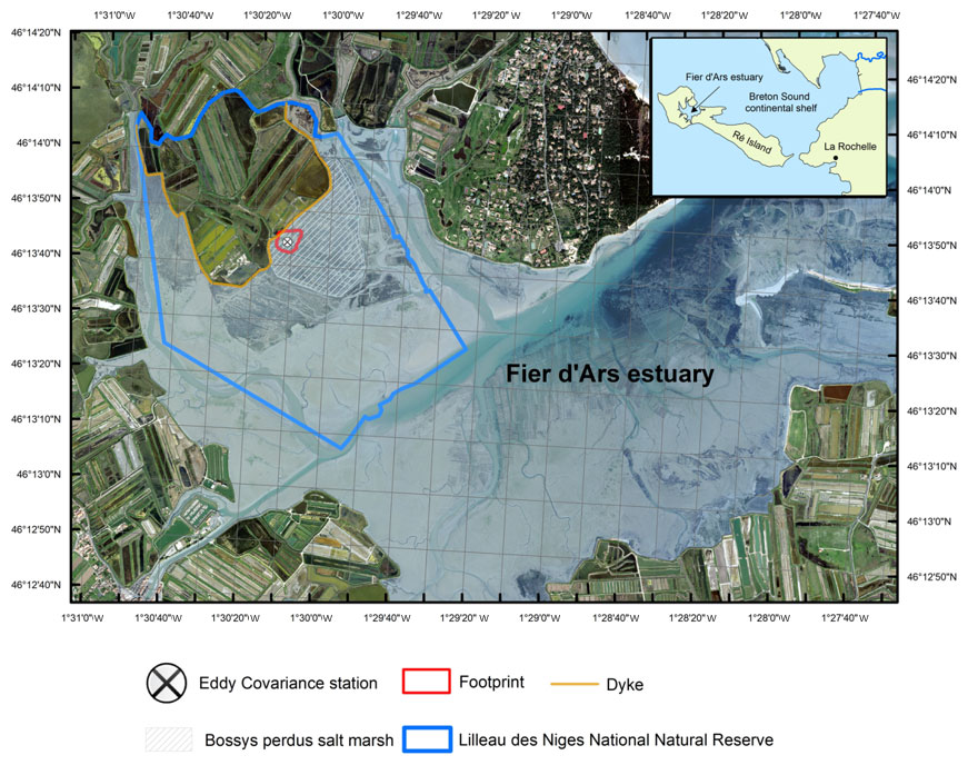
Figure 1 The studied Bossys perdus salt marsh located on the French Atlantic coast within the National Natural Reserve (blue line delimitation) on Ré Island. The salt marsh is connected to the Fier d'Ars tidal estuary (light blue). The dyke separates terrestrial and maritime marsh areas (orange line). The eddy covariance system and associated estimated footprint are indicated (black cross and red line; see Fig. 2). From geo-referenced IGN 2019 orthogonal images (Institut national de l'information géographique et forestière (IGN)).

Our study focused on the atmospheric CO₂ uptake capacity of a tidal salt marsh (old anthropogenic marsh) under the influence of biophysical factors and its potential role in global and regional C budgets. For this purpose, we deployed an atmospheric EC station to measure vertical CO₂ fluxes (NEE) during the year 2020 at the ecosystem scale on the Bossys perdus salt marsh on Ré Island connected to the French continental shelf of the Atlantic Ocean. Here, we aim to (a) describe NEE flux temporal series measured at different temporal scales (diurnal, tidal and seasonal scales) using the EC technique, (b) evaluate the relevant environmental factors that control atmospheric CO₂ exchanges (i.e. NEE) and (c) accurately qualify and quantify the effects of tides on the marsh CO₂ metabolism.

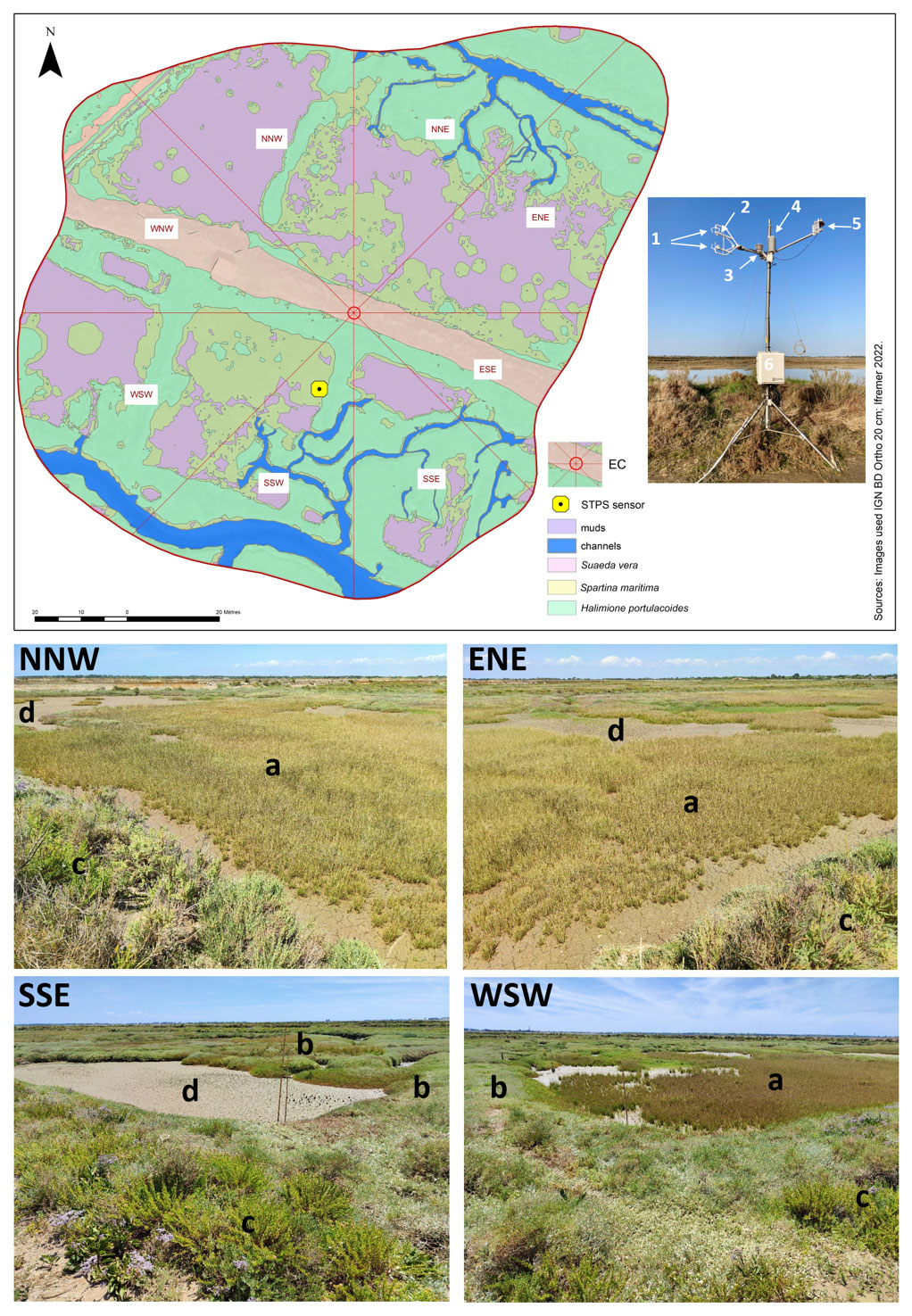
Figure 2 Location and set-up of the eddy covariance (EC) system within the Bossys perdus salt marsh and its associated footprint estimated from Kljun et al. (2015) and averaged over the year 2020 (70 % contour line, i.e. 13 042 m²). Wind sectors (45°) and marsh habitats (see Table 1) are represented. The canopy height of the studied marsh is short and constant (from 0.15 m for H. portulacoides to 0.30 m for S. maritima). The STPS sensor (in yellow), measuring water heights (H_w) and temperatures (T_w), was located in the SSW sector. The EC system (Campbell Scientific) includes (1) the ultrasonic anemometer (CSAT3), (2) the open-path infrared gas analyser (EC150), (3) the temperature probe (100K6A1A thermistor), (4) the temperature/relative humidity sensor (HMP155A), (5) the silicon quantum sensor (SKP215) and (6) the central acquisition system (CR6) and the electronics module (EC100). A rainfall sensor (TE525MM; Rain Gauge, Texas Electronics) simultaneously measured the cumulative precipitation. From geo-referenced IGN 2019 orthogonal images. Photographs of four wind sectors within the studied footprint area (NNW, ENE, WSW and SSE) were taken from the EC system during an emersion period in summer 2021 when all the marsh habitats were emerged into the atmosphere: (a) Spartina maritima, (b) Halimione portulacoides, (c) Suaeda vera and (d) mudflat. © S.-C. Zech.

2 Materials and methods

2.1 Study site

The study was conducted at the Bossys perdus salt marsh situated along the French Atlantic coast on Ré Island (Fig. 1). It corresponds to a vegetated intertidal area of 52.5 ha that has been protected inside the National Natural Reserve (NNR) (Fig. 1). Between the 17th and most of the 20th century, the salt marsh experienced successive periods of intensive land use (salt harvesting and oyster farming) and returned to natural conditions before becoming a permanent part of the NNR in 1981 for the biodiversity protection without major restoration work (Julien Gernigon, personal communication, 2023). It is currently managed to restore its natural hydrodynamics while conserving the site's specific typology due to past human activities (channel networks, humps and dykes; Fig. 2). This salt marsh is linked to the Fier d'Ars tidal estuary that exchanges between 2.4 and 10.2 ×10⁶ m³ of coastal waters with the Breton Sound continental shelf allowing a maximal tidal range of 5 m in the estuary (Bel Hassen, 2001). This communication allows (1) drainage of the intertidal zone of the estuary including mudflats (Mayen et al., 2023) and tidal salt marshes (Mayen et al., 2023) and (2) supply of coastal water to a large complex of artificial salt marshes (i.e. salt ponds) located upstream of the dyke (Fig. 1). The artificial marsh waters managed by the NNR for biodiversity protection (Mayen et al., 2023) are flushed back to the estuary downstream through the Bossys perdus channel (Fig. 1).

The Bossys perdus salt marsh, located upstream of the estuary (Mayen et al., 2023), is subjected to semi-diurnal tides from the Breton Sound continental shelf (Fig. 1) allowing the marsh immersion by two main channels differently in space, time and frequency according to the tidal periods (Fig. 2). At high tide, advected coastal waters can completely fill channels (Fig. S1b in the Supplement) and immerse the marsh through variable water heights depending on tidal amplitudes and meteorological conditions (Fig. S1c). In contrast, at low tide, the marsh vegetation at the benthic interface is emerged into the atmosphere without any coastal waters (Fig. S1a). During this time, Bossys perdus channels allow drainage of upstream artificial marsh waters to the estuary (Fig. 2). The marsh vegetation assemblage was mainly composed by three halophytic species as perennial plants (Halimione portulacoides, Spartina maritima and Suaeda vera; Fig. 2) that associated with different metabolic pathways (the C₃-type photosynthesis for H. portulacoides and S. vera and the C₄-type photosynthesis for S. maritima; Duarte et al., 2013, 2014). Whereas H. portulacoides and S. vera are evergreen plants throughout the year, the growing season for S. maritima was shorter (from spring) with a flowering period between August and October (plants persist only in the form of rhizomes in winter and fall; Julien Gernigon, personal communication, 2023).

2.2 Eddy covariance and micrometeorological measurements

The atmospheric eddy covariance technique allowed us to quantify the net CO₂ fluxes at the ecosystem–atmosphere interface through micrometeorological measurements of the vertical component of atmospheric turbulent eddies (Aubinet et al., 2000; Baldocchi, 2003; Burba, 2021). The averaged vertical flux of any gas (F, µmol m⁻² s⁻¹) can be expressed as the covariance between the vertical wind speed (w, m s⁻¹), air density (ρ, kg m⁻³) and the dry mole fraction (s) of the gas of interest as

$$\begin{array}{}\text{(1)}& F=\stackrel{\mathrm{‾}}{\mathit{\rho }ws}\approx \stackrel{\mathrm{‾}}{\mathit{\rho }}\stackrel{\mathrm{‾}}{w^{\prime }{s}^{\prime }},\end{array}$$

where the overbar represents the time average of the parameter (i.e. 10 min in this study due to strong fluctuations at the tidal scale; Polsenaere et al., 2012) and the prime indicates the instantaneous turbulent fluctuations in these parameters relative to their temporal average (Reynolds, 1883). The Reynold's decomposition was used to break the instantaneous term down into its mean and deviation (e.g. w = $\stackrel{\mathrm{‾}}{w}+w^{\prime }$) (Reynolds, 1883; Burba, 2021). This equation (Eq. 1) is obtained by assuming, on a flat and homogeneous surface, that (1) the variation in air density is negligible, (2) there is no divergence or convergence of large-scale vertical air motion and (3) atmospheric conditions are stable and stationary (Aubinet et al., 2012). A negative flux of atmospheric CO₂ is directed towards the ecosystem, and is therefore characterized as a sink, and vice versa for positive fluxes qualified as sources of CO₂ to the atmosphere.

Table 1 Bossys perdus marsh habitat (percentages are in bold and associated surface area, in square metres, are in brackets) within each 45° wind sector in the corresponding footprint areas (Fig. 2) and the whole averaged footprint for the year 2020 (13 042 m², 70 % contour line).

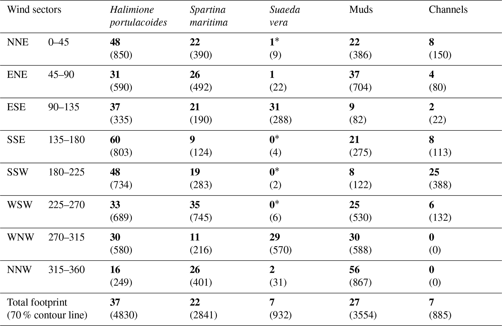
^∗ Negligible surfaces on the total area of the sector.

An EC system was continuously deployed at the Bossys perdus salt marsh to measure the net ecosystem CO₂ exchange (NEE, µmol m⁻² s⁻¹). The set of EC sensors (Fig. 2), at a height of 3.15 m, was composed of an open-path infrared gas analyser (model EC150; Campbell Scientific) to measure the CO₂ (mg m⁻³) and H₂O (g m⁻³) concentrations in the air as well as the atmospheric pressure (kPa) and an ultrasonic anemometer (model CSAT3; Campbell Scientific) to measure the three-dimensional components of wind speed (U, V and W; m s⁻¹) at a frequency of 20 Hz and averaged every 10 min (Fig. 2). The EC150 gas analyser also measured the air temperature using a thermistor probe (model 100K6A1A; BetaTherm). The EC100 electronics module (model EC100; Campbell Scientific) allowed us to synchronize high-frequency measurements and rapid communications between the CR6 datalogger (model CR6; Campbell Scientific) and EC devices including EC150 and CSAT3A (Fig. 2). The CR6 datalogger is a powerful core component for the data acquisition system. Additional meteorological data, such as relative humidity (RH, %), air temperature (T_a, °C) and photosynthetically active radiation (PAR, µmol m⁻² s⁻¹), were recorded every 10 min simultaneously and at the same height as the EC sensors, by a temperature/relative humidity sensor (HMP155A; Campbell Scientific), with RAD14 natural ventilation shelter) and a silicon quantum sensor (SKP215; Skye Instruments), respectively (Fig. 2). The vapour pressure deficit (VPD, Pa) was calculated every 10 min from saturated vapour pressure (calculated from T_a) and from actual vapour pressure (calculated from RH). A rainfall sensor (TE525MM; Rain Gauge, Texas Electronics), located 10 m away and connected to the EC station, simultaneously measured the cumulative precipitation at a height of 1 m (rainfall, mm). All high-frequency EC data were recorded on an SD micro-card (2 Go; Campbell Scientific) that was replaced every 2 weeks, whereas meteorological data were recorded and stored in the central acquisition system (CR6). The EC system was connected to two rechargeable batteries (12 volts and 260 A h⁻¹; AGM) powered by a monocrystalline solar panel (24 V, 200Wp module with MPPT 100 V/30 A controller; Victron Energy). The EC sensors were checked and cleaned every 2 weeks and the EC150 was calibrated each season with a zero-air calibration of 0 ppm (Campbell Scientific) and a certificated CO₂ standard of 520 ppm (Gasdetect). Water height (H_w; ± 0.3 m) and water temperature (T_w; ± 0.1 °C) were also measured every 10 min along with EC data using a STPS probe (NKE Instrumentation) located 20 m away from the EC system (Fig. 2). The sensor was checked every two months at the laboratory to verify possible derivations in the measured parameters.

2.3 Footprint estimation and immersion/emersion marsh heterogeneity

Footprints were estimated using the model of Kljun et al. (2015) applied to data from the year 2020 to obtain an annual averaged footprint from the constant measurement height (Z_m = 3.15 m), the constant displacement height (d = 0.1 m; estimated from 0.67 times the canopy height; LI-COR, EddyPro^® 7 Software, LI-COR Environmental), mean wind velocities (u_mean, m s⁻¹), standard deviations of the lateral velocity fluctuations after rotation (sigma_v, m s⁻¹), the Obukhov length (L), friction velocities (u^∗, m s⁻¹) and wind directions (°) obtained from the EC measurements and the processing software (EddyPro^® v7.0.8; LI-COR) output. For verification, we performed the footprint estimations both with variable Z_m from water height measurements and with constant Z_m from data at emersion and we obtained the same footprint shapes and extends. For all calculations (i.e. habitat coverage, relationships with CO₂ fluxes, etc.), we used the 70 % footprint contour line that corresponds to an average footprint of 13 042 m² of the studied salt marsh area of interest (Fig. 2). A land-use map was also created (Fig. 2) from geo-referenced IGN BD orthogonal images with a resolution of 20 cm (2019) using ArcGIS 10.2 (ESRI). The spatial analysis tool of ArcGIS 10.2 was used to perform an unsupervised classification of the BD orthogonal images. We checked the resulting map by selecting 20 random locations within the footprint of the studied salt marsh and compared their land use on the ground and on the map.

In some situations, based on the tide (neap tides), due to meteorology influence (wind direction and atmospheric pressure) and the local altimetry heterogeneity, our one-location H_w measurements could not accurately account for the whole spatial emersion and immersion of the marsh in the EC footprint (Fig. 2). At incoming tide, when coastal waters begin to fill the channel and then overflow over the marsh (from 0.5 h in spring tides to 2.5 h in neap tides; data not shown), the SSW sector (Fig. 2) was first immersed and a non-zero H_w value was measured. However, although some marsh sectors were immersed at the same time, others were still emerged. Indeed, lowest marsh levels (56 % of the footprint area), mainly composed of mudflats and S. maritima (Fig. 2; Table 1), were quickly immersed from H_w > 0 m (south), whereas the whole marsh immersion (muds and plants) only occurred 0.75 h later from H_w > 1.0 m at high tide during spring tide. Thus, the highest marsh levels (44 % of the footprint area), mainly composed of H. portulacoides and S. vera (Fig. 2; Table 1), were still emerged for 0 < H_w < 1.0 m. Conversely, at neap tide, this footprint immersion versus emersion marsh heterogeneity could still be present even at high tide due to insufficient water levels. Although a digital field model for water heights could not be performed in 2020 to have a better spatial representation of the immersion/emersion footprint, all these important considerations were considered in our computations and analyses in this study.

2.4 EC data processing and quality control

Raw EC data measured at high-frequency were processed following Aubinet et al. (2000) with the EddyPro software. First, different correcting steps were applied to our raw data according to the procedures given by Vickers and Mahrt (1997) and Polsenaere et al. (2012) for intertidal systems: (1) unit conversion to check that the units for instantaneous data are appropriate and consistent to avoid any errors in the calculation and correction of CO₂ fluxes; (2) despiking to remove outliers in the instantaneous data from the anemometer and gas analyser due to electronic and physical noise and replaced the detected spikes with a linear interpolation of the neighbouring values; (3) amplitude resolution to identify situations in which the signal variance is too low with respect to the instrumental resolution; (4) double coordinate rotation to align the x axis of the anemometer to the current mean streamlines, nullifying the vertical and cross-wind components; (5) time delay removal by detecting discontinuities and time shifts in the signal acquisition from the anemometer and gas analyser; (6) detrending with removal of short-term linear trends to suppress the impact of low-frequency air movements; and (7) performing the Webb–Pearman–Leuning (WPL) correction to take into account the effects of temperature and water vapour fluctuations on the measured fluctuations in the CO₂ and H₂O densities (Burba, 2021). The turbulent fluctuations of CO₂ fluxes were calculated with EddyPro using the linear detrending method (Gash and Culf, 1996) which involves calculating deviations from around any linear trend evaluated (i.e. over the whole flux averaged period). High-frequency CO₂ fluxes were processed and averaged over intervals of 10 min (shorter than in terrestrial ecosystems) to detect fast NEE variations with the tide (Polsenaere et al., 2012; Van Dam et al., 2021). During the EC data processing by EddyPro, a correction for flux spectral losses in the low frequency range was performed according to Moncrieff et al. (2004).

A strict quality control was applied on EddyPro processed CO₂ flux data to remove bad data related to instrument malfunctions, processing and mathematical artefacts, ambient conditions that do not satisfy the requirements for the EC method, wind that is not from the footprint and heavy precipitation for the open-path IRGA (Burba, 2021). Processed data were screened using tests for steady state and turbulent conditions (Foken and Wichura, 1996; Foken et al., 2004; Göckede et al., 2004). In this study, we did not apply a ustar filter in our EC data processing because we measured only 11 % of night-time data corresponding to a ustar threshold below 0.1 m s⁻¹ and above which NEE does not increase anymore with ustar values (threshold close to values found in grassland; Gu et al., 2005). Contrary to terrestrial ecosystems (Gu et al., 2005), the low canopy height of the studied marsh strongly limited the CO₂ storage in the vegetation and favours the atmospheric CO₂ circulation. If the signal to noise ratio of the EC150 gas analyser was less than 0.7 and/or the percentage of high-frequency missing values over 10 min exceeded 10 % (i.e. data absent in the raw data file or removed through the quality screening procedures), no flux was calculated. This choice was the best compromise between removing poor-quality data and keeping as much of measured CO₂ flux data as possible (data and associated tests not shown). Then, we used the method of Papale et al. (2006) to detect and remove outliers in the 10 min flux data. The median and median absolute deviation (MAD) were calculated over a 2-week window separating daytime and night-time periods. Data above 5.2× MAD were removed. After all post-processing and quality controls, 18.3 % of the EC data were removed and gap-filled through a machine learning approach to obtain continuous flux data in 2020.

2.5 Flux gap filling and statistic tools

The random forest (RF) model was used to gap-fill our EC dataset. Random forest is a supervised machine learning technique proposed by Breiman (2001) that can model a non-linear relationship with no assumption about the underlying distribution of the data population. This method has been shown to be particularly suited to gap-fill EC data (Kim et al., 2020; Cui et al., 2021). Random forest builds multiple decision trees, each of which is based on a bootstrap aggregated data sample (i.e. bagging of the EC data) and a random subset of predictors (i.e. the selected environmental data; Table S1 in the Supplement). We build RF models with environmental predictors that have been identified in the literature to control CO₂ fluxes in salt marshes and which were available during the gaps and with measurements recorded between 2019 and 2020 (Table S1). Each random forest model was built from a trained bagging ensemble of 400 randomly generated decision trees (Kim et al., 2020) with the “randomForest” package in the R software (Liaw and Wiener, 2022). In this study, we used the RF2 model with PAR, air temperature, water height and relative humidity as environmental predictors because its performance indicators showed a high Pearson correlation coefficient (R² = 0.88) and low values of root mean square error (RMSE = 1.27) and model bias (0.0024) allowing us to correctly gap-fill a large EC data (Table S1). The calculated uncertainty of the RF2 model on the resulting annual C budget was 0.43 %. Each tree was trained from bagged samples including 70 % of the initial dataset. The remaining 30 % of the data were used to estimate the fit of each random forest model. The model used was then able to explain 88 % of the variability in the test data. Daytime data were better explained than night-time data (59 % vs. 38 %), with light being the main parameter of the model. However, only 20 % of the night-time EC data were gap-filled with the random forest model. Using a partial dependence analysis and an ondelette analysis, we concluded that the relationships and temporal dynamics modelled allowed us to correctly fill the gaps in our dataset. However, extreme values of some predictors (i.e. PAR > 1000 µmol m⁻² s⁻¹) can reduce the random Forest model performance for estimation of EC data. This observation is common for random forest models, as they show poor results for extreme values. Other models, such as artificial neural networks, were also tested but showed poorer results (Table S1).

For all measured variables, the 10 min data did not follow a normal distribution (Shapiro–Wilk tests, p < 0.05). Non-parametric comparisons, such as the Mann–Whitney and Kruskal–Wallis tests, were carried out with a 0.05 level of significance. To assess the influence of meteorological and hydrological drivers on NEE fluxes at different temporal scales, we performed a pairwise Spearman's correlation analysis on the 10 min values and monthly mean values (“cor function” in R).

2.6 Temporal analysis of NEE fluxes and partitioning

During the year 2020, temporal variations in NEE fluxes were studied at the seasonal and diurnal/tidal scales. Seasons were defined based on calendar dates: the winter period from 1 January 2020 to 19 March 2020 and from 21 to 31 December 2020, the spring period from 20 March 2020 to 19 June 2020, the summer period from 20 June 2020 to 21 September 2020 and the fall period from 22 September 2020 to 20 December 2020. Daytime and night-time were separated into PAR > 10 and PAR ≤ 10 µmol m⁻² s⁻¹, respectively. For the NEE flux analysis according to environmental drivers, NEE fluxes were grouped into five PAR groups (0 < PAR ≤ 10, 10 < PAR ≤ 500, 500 < PAR ≤ 1000, 1000 < PAR ≤ 1500 and 1500 < PAR ≤ 2000 µmol m⁻² s⁻¹) to reduce NEE fluctuations due to PAR variations. Water heights (H_w) measured at one location over the marsh (Fig. 2) relative to the mean sea level were used to distinguish emersion (H_w = 0 m at low tide) and immersion (H_w > 0 m at high tide) periods (see Sect. 2.3) and thus, the influence of tides on NEE fluxes.

To study marsh metabolism related to photosynthesis and respiration processes, measured NEE fluxes were partitioned into gross primary production (GPP) and ecosystem respiration (R_eco), respectively. During marsh emersion, NEE fluxes occur at the marsh–atmosphere interface involving only benthic metabolism (or marsh metabolism) resulting in NEE = GPP−R_eco. During marsh immersion, NEE fluxes are the result of benthic metabolism, planktonic metabolism and lateral C exchanges by tides thereby making it more difficult to study the marsh metabolism (Polsenaere et al., 2012). Negative NEE values indicated a marsh CO₂ uptake from the atmosphere and positive values indicated a marsh CO₂ source into the atmosphere. GPP was expressed in negative values and R_eco was expressed in positive values. In this study, NEE flux partitioning into marsh metabolic fluxes (NEE_marsh) was performed according to the following equation using the model of Kowalski et al. (2003):

$$\begin{array}{}\text{(2)}& {\mathrm{NEE}}_{\mathrm{marsh}}=\mathrm{GPP}-R_{\text{eco}}={\displaystyle \frac{a_{\mathrm{1}}\mathrm{PAR}}{a_{\mathrm{2}}+\mathrm{PAR}}}-R_{\text{eco}},\end{array}$$

where a₁ is the maximal photosynthetic CO₂ uptake at light saturation (µmol CO₂ m⁻² s⁻¹) and a₂ is the PAR at half of the maximal photosynthetic CO₂ uptake (µmol photon m⁻² s⁻¹). The $a_{\mathrm{1}}/a_{\mathrm{2}}$ ratio corresponds to photosynthetic efficiency (Kowalski et al., 2003). R_eco was calculated as follows according to Wei et al. (2020b):

$$\begin{array}{}\text{(3)}& R_{\text{eco}}=R_{\mathrm{0}}\text{exp}\left(b{T}_{\mathrm{a}}\right),\end{array}$$

where R_eco is the night-time ecosystem respiration (µmol CO₂ m⁻² s⁻¹), R₀ is the ecosystem respiration rate at 0 °C (µmol CO₂ m⁻² s⁻¹), T_a is the air temperature (°C) and b is a response coefficient of the temperature variation (Wei et al., 2020b).

For NEE flux partitioning, estimations of the GPP coefficients (a₁ and a₂; Eq. 2) and R_eco coefficients (R₀ and b; Eq. 3) were performed by the least squares method (“minpack.lm” package in R) at the monthly scale only during emersion periods where measured NEE fluxes corresponded to estimated NEE_marsh fluxes. First, for each month, R₀ and b were estimated during night-time emersion periods where NEE = R_eco following Eq. (3) (Wei et al., 2020b). Then, a₁ and a₂ were estimated during daytime emersion periods using night-time respiration coefficients (R₀ and b) where NEE = GPP−R_eco following Eqs. (2) and (3) (Kowalski et al., 2003). Finally, NEE_marsh (net marsh metabolic fluxes without tidal influence) were calculated from PAR and T_a values measured at a 10 min frequency throughout the year using the monthly coefficients calculated for the partitioning (Eq. 2). As our ecosystem had a low phenological variation (Table S2), we concluded that a monthly time step for the coefficient estimation was sufficient to answer our study objectives. During emersion periods, monthly net C balances (i.e. budgets) of measured NEE and estimated NEE_marsh, as well as the monthly mean fluxes, were very similar (Table S3), confirming the correct NEE flux partitioning calculations done in this study.

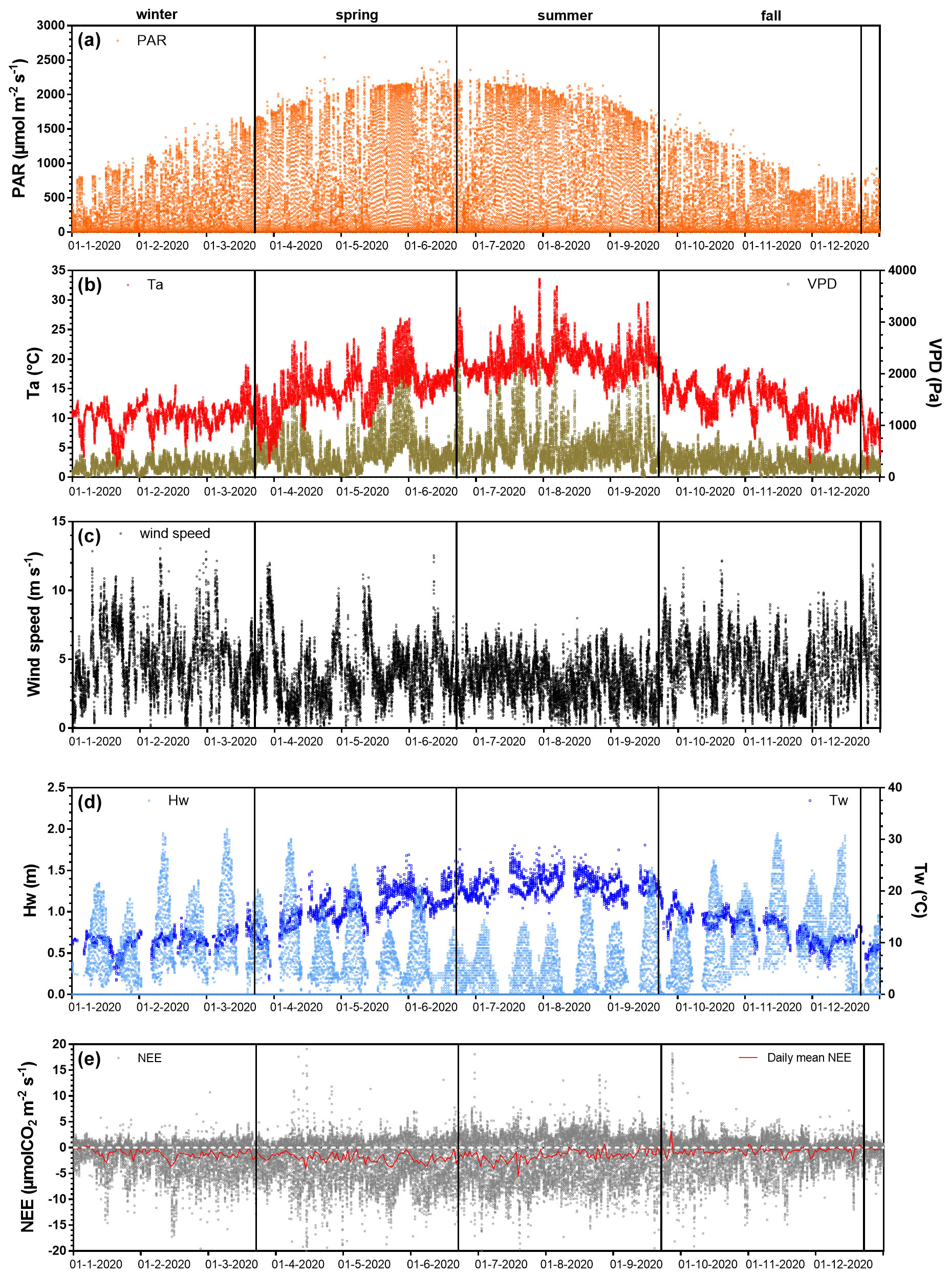
Figure 3 Net ecosystem exchanges and associated environmental parameters measured every 10 min throughout the year 2020. The measured environmental parameters include (a) the photosynthetically active radiation (PAR, µmol m⁻² s⁻¹), (b) air temperature (T_a, °C), vapour pressure deficit (VPD, Pa), (c) wind speed (m s⁻¹), (d) water height (H_w, m), water temperature (T_w, °C) and (e) the net ecosystem exchanges (NEE, µmol CO₂ m⁻² s⁻¹) computed from the 20 Hz atmospheric CO₂ and wind speed measurements with the EddyPro software. The red line in (e) is the moving average of NEE (daily mean). Seasons are delimited by vertical lines.

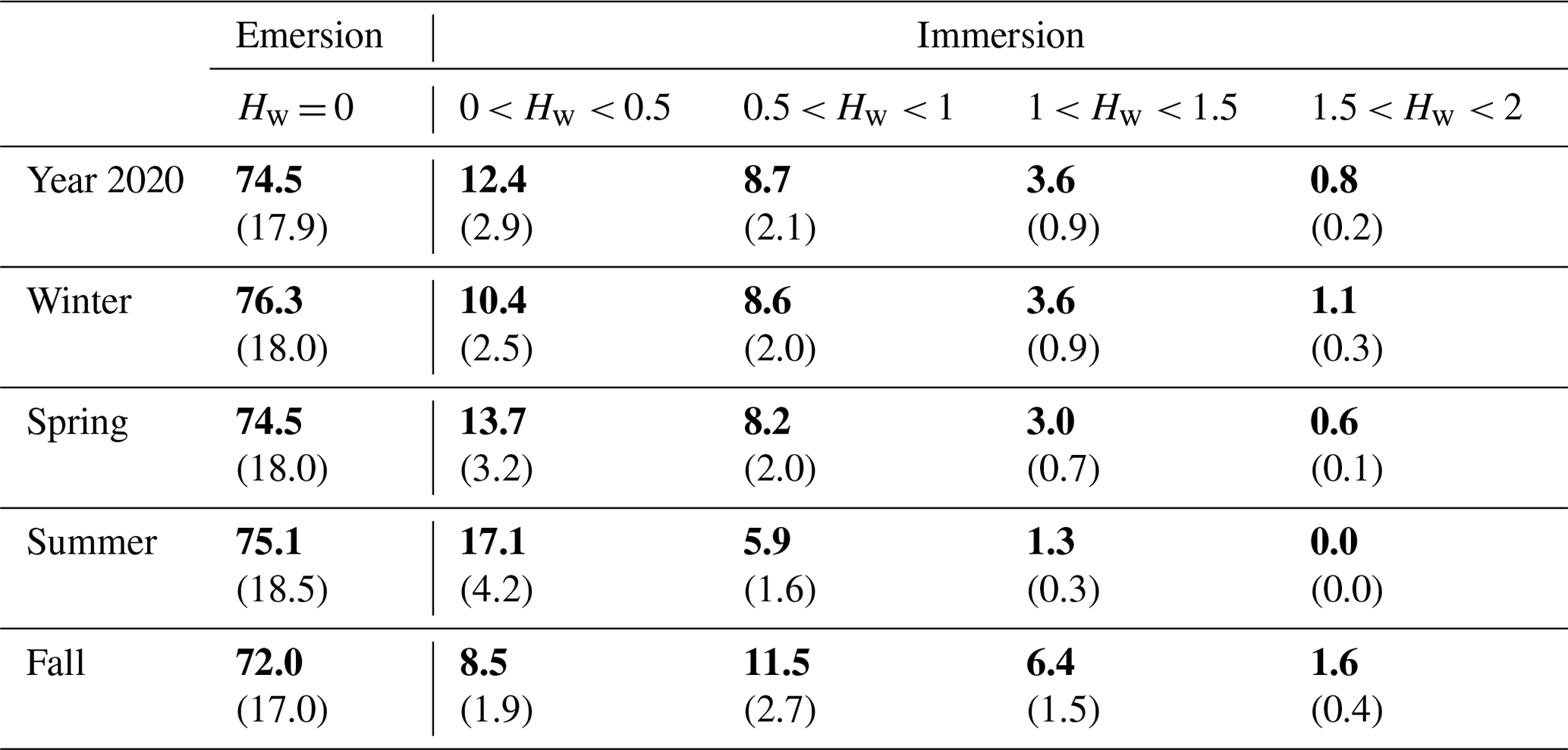
Table 2 Emersion and immersion periods (percentage in bold) at the studied salt marsh for four water height ranges of 0.5 m during the year 2020 and at the seasonal scale. The emersion and immersion durations in hours per day were calculated (shown in brackets).

3 Results

3.1 Habitat covering of the footprint

Within the EC footprint, halophyte marsh vegetation (66 %) composed of Halimione portulacoides, Spartina maritima and Suaeda vera mainly dominated, whereas muds and channels only accounted for 27 and 7 %, respectively (Fig. 2). The area occupied by S. vera, crossing the EC footprint from WNW to ESE (Table 1), corresponded to the highest marsh level that was partly immersed only during the highest tidal amplitudes (Fig. 2). H. portulacoides and S. maritima occupied mostly the NNE (70 %), SSE (69 %), WSW (68 %) and SSW (67 %) wind sectors. In contrast, mud habitats mostly covered the NNW sector, where the lowest vegetation cover was found (Fig. 2; Table 1). The highest channel area was found in the SSW sector (Fig. 2; Table 1).

3.2 Seasonal variations in environmental conditions and NEE fluxes

Throughout the year 2020, the full seasonal range in solar radiation was measured (Fig. 3a) with an increase in daytime PAR from winter (lowest light season) to summer (brightest season). A similar seasonal pattern was recorded for air temperatures (T_a) with values ranging from 1.5 °C in winter (coldest season) to 33.6 °C in summer (warmest season; Fig. 3b). On average, the winter and fall seasons were the wettest (RH > 82 %), associated with the lowest vapour pressure deficit (VPD) values, whereas spring and summer were the driest ones (RH < 75 %), associated with the highest VPD values (Fig. 3b). Indeed, the highest and lowest cumulative rainfalls were recorded in fall (342 mm) and summer (62 mm), respectively. The highest mean seasonal wind speed was measured in winter (4.9 ± 2.3 m s⁻¹) with maximal speeds up to 13 m s⁻¹ (Fig. 3c). Winds came mostly from the SSW–WSW sectors both in winter (55 %) and summer (41 %) and from the NNE–ENE sectors both in spring (51 %) and fall (31 %) (Fig. 2). Tidal activities reflected the typical hydrological conditions of the Atlantic coasts with a bi-monthly succession of spring tides and neap tides (Fig. 3d). Water heights (H_w) strongly varied according to tidal amplitudes with a maximal H_w of 1.4 m during neap tides and 2.0 m during spring tides (overall annual mean of 0.6 ± 0.4 m; Fig. 3d). Throughout the year, 25.5 % of the EC data were measured when the salt marsh was immersed through variable immersion durations and water heights (Table 2). On average, the daily immersion durations ranged between 5.7 h d⁻¹ in winter (23.7 % of the EC data) and 6.5 h d⁻¹ in fall (28 % of the EC data). In winter, the EC data during immersion were split into 19 % for 0 < H_w < 1 m and 4.7 % for 1 < H_w < 2 m, whereas in fall, these latter were split into 20 % for 0 < H_w < 1 m and 8 % for 1 < H_w < 2 m. In summer, the lowest marsh immersion was measured with no H_w value higher than 1.5 m (Table 2).

The annual mean NEE value was −1.27 ± 3.48 µmol m⁻² s⁻¹ with strong temporal variabilities recorded over both long and short timescales (Fig. 3e). Significant NEE variations were highlighted between each season (Kruskal–Wallis test, p < 0.001) where, on average, the highest and lowest atmospheric CO₂ sinks were recorded in spring (−1.93 ± 3.84 µmol m⁻² s⁻¹) and fall (−0.59 ± 2.83 µmol m⁻² s⁻¹), respectively (Fig. 4). NEE flux partitioning gave an annual mean NEE_marsh value of −1.28 ± 3.16 µmol m⁻² s⁻¹, ranging from −2.00 ± 3.49 µmol m⁻² s⁻¹ in spring to −0.53 ± 2.51 µmol m⁻² s⁻¹ in fall. On average, in winter and fall, the measured NEE values were more negative than the estimated NEE_marsh values, whereas in spring and summer, the opposite trend was recorded (Fig. 4). Contrary to NEE and NEE_marsh, the highest seasonal values of GPP and R_eco were estimated in summer, whereas the lowest seasonal values were estimated in winter (Fig. 4). The highest and lowest photosynthetic efficiencies ($a_{\mathrm{1}}/a_{\mathrm{2}}$ ratio) were found in winter (−2.08 × 10⁻²) and summer (−1.36 × 10⁻²), respectively.

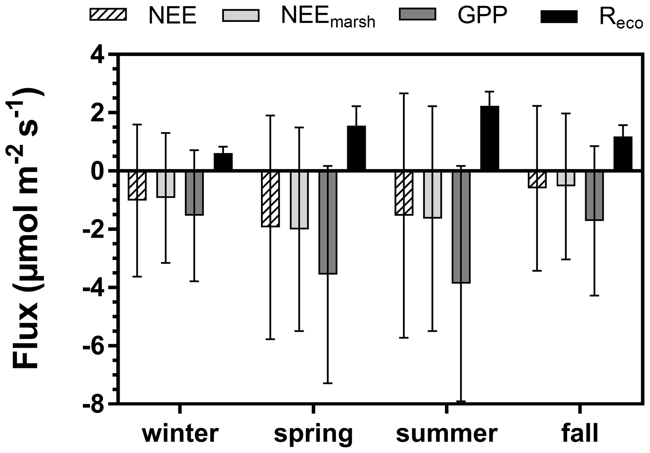
Figure 4 Seasonal variations (means ± SD) of the measured NEE, estimated NEE_marsh, estimated GPP and estimated R_eco (µmol CO₂ m⁻² s⁻¹) recorded throughout the year 2020. NEE: net ecosystem exchange, NEE_marsh: net ecosystem exchange at the marsh–atmosphere interface without coastal water, GPP: gross primary production, R_eco: ecosystem respiration. The NEE fluxes were partitioned into GPP and R_eco according to Kowalski et al. (2003) and Wei et al. (2020b) (see Sect. 2.6).

Table 3 Diurnal/tidal variations (means ± SD in bold) of NEE fluxes (µmol CO₂ m⁻² s⁻¹) during each season in 2020. The associated ranges (min/max) are indicated in brackets. Daytime and night-time periods were separated into PAR > 10 and PAR ≤ 10 µmol m⁻² s⁻¹, respectively, whereas emersion and immersion periods were separated into H_w = 0 m and H_w > 0 m, respectively.

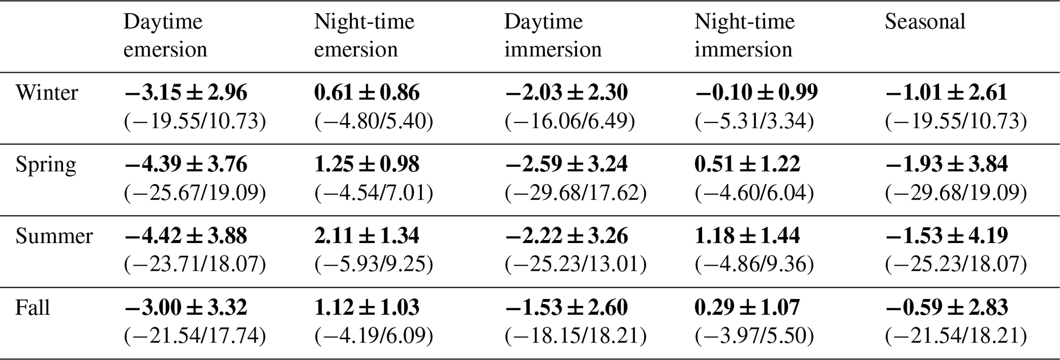
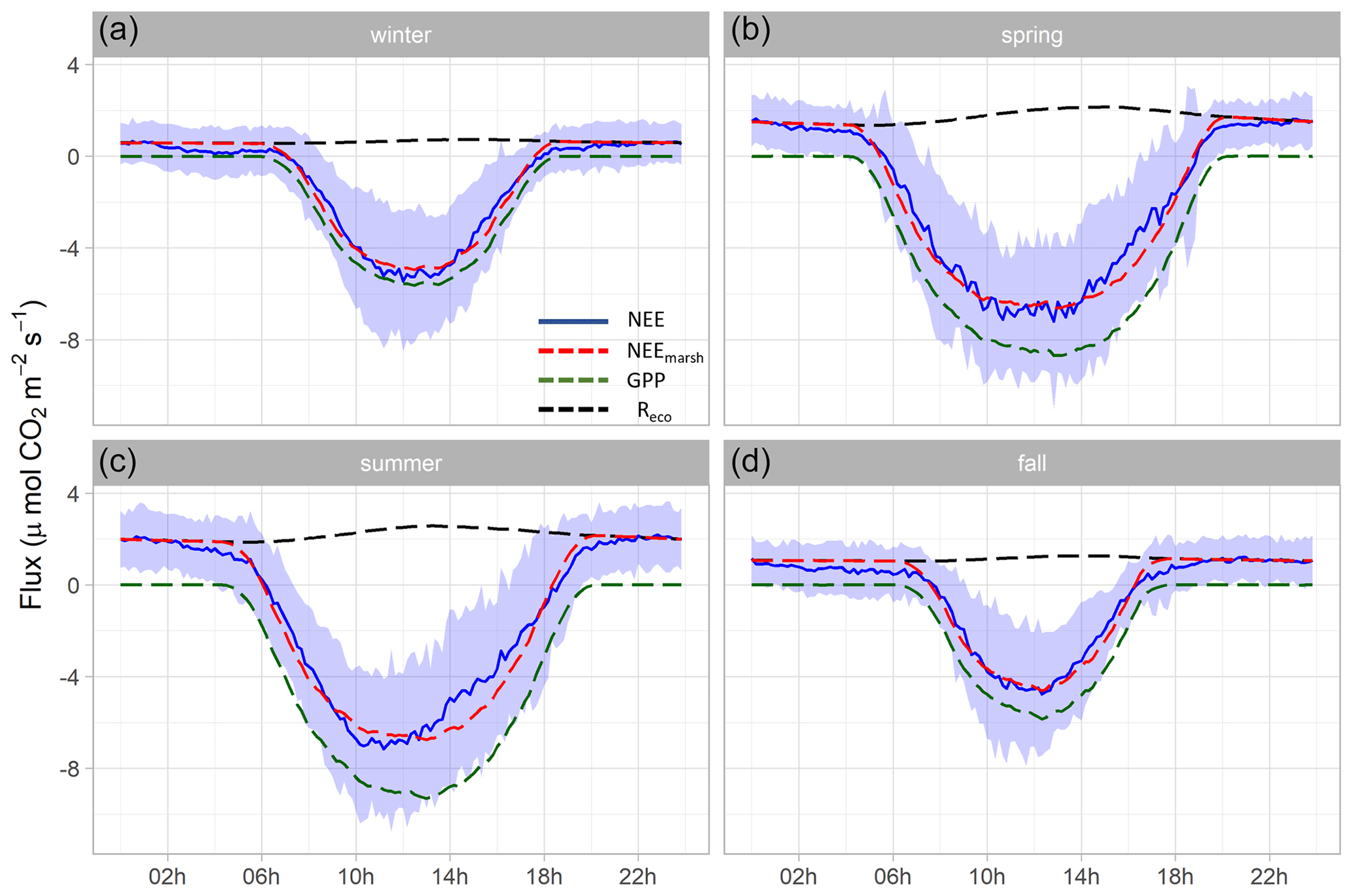
Figure 5 Hourly plots of the measured NEE, estimated NEE_marsh, estimated GPP and estimated R_eco diurnal variations obtained every 10 min in winter (a), spring (b), summer (c) and fall (d) for the year 2020. NEE averages are represented by solid blue lines and standard deviations are represented by blue areas. The NEE_marsh, GPP and R_eco averages are represented by dotted red, green and black lines, respectively. The measured NEE fluxes were partitioned into GPP and R_eco according to Kowalski et al. (2003) using monthly coefficients (see the “Materials and methods” section). Night-time periods correspond to GPP = 0 µmol m⁻² s⁻¹ and NEE_marsh = R_eco. All values are in µmol CO₂ m⁻² s⁻¹.

3.3 Environmental parameter and NEE flux variations at diurnal and tidal scales

At each season, significant diurnal differences in NEE fluxes were highlighted (Mann–Whitney tests, p < 0.05) with, on average, an atmospheric CO₂ sink during daytime and an atmospheric CO₂ source during night-time, irrespective of emersion or immersion periods (Table 3). For instance, in spring, NEE means were −3.93 ± 3.72 and 1.06 ± 1.09 µmol m⁻² s⁻¹ during daytime and night-time, respectively (Fig. 5b). Over all seasons, similar diurnal variations in measured NEE and estimated NEE_marsh were recorded with, on average, a rapid increase in CO₂ uptake during the morning up to the middle of the day (low T_a and VPD values) and then, a decrease in CO₂ uptake during the afternoon (high T_a and VPD values) to become a CO₂ source during night-time (Figs. 5 and S2). On average, during the afternoon, the GPP decreases and R_eco increases explained the measured decrease in CO₂ uptake (Fig. 5). For each season, the highest marsh CO₂ uptakes were measured during daytime emersion periods between 12:00 and 13:00 UT (maximal PAR levels), with the latter increasing from winter (−4.84 ± 2.87 µmol m⁻² s⁻¹) to spring–summer (−6.94 ± 2.80 µmol m⁻² s⁻¹; Fig. 5).

At each season, the tidal rhythm strongly disrupted NEE fluxes with, in general, no change in the marsh metabolism status (sink/source). During daytime, significantly lower CO₂ uptakes were recorded during immersion than during emersion (Mann–Whitney tests, p < 0.05) when marsh plants were mostly immersed in tidal waters, and during night-time, a similar tidal pattern was recorded for CO₂ emissions (Mann–Whitney tests, p < 0.05; Table 3). For instance, in spring, NEE means were −4.39 ± 3.76 and −2.59 ± 3.24 µmol m⁻² s⁻¹ during daytime emersion and daytime immersion, respectively, and were 1.25 ± 0.98 and 0.51 ± 1.22 µmol m⁻² s⁻¹ during night-time emersion and night-time immersion, respectively. In winter, during some night-time periods, weak CO₂ sinks were recorded both during emersion (−0.79 ± 0.84 µmol m⁻² s⁻¹; 137 h over 71 d) and immersion (−0.82 ± 0.91 µmol m⁻² s⁻¹; 143 h over 55 d associated with a mean H_w of 0.80 m; Fig. S2). The maximal CO₂ uptakes were −4.80 and −5.31 µmol m⁻² s⁻¹ during night-time emersion and night-time immersion, respectively (Table 3).

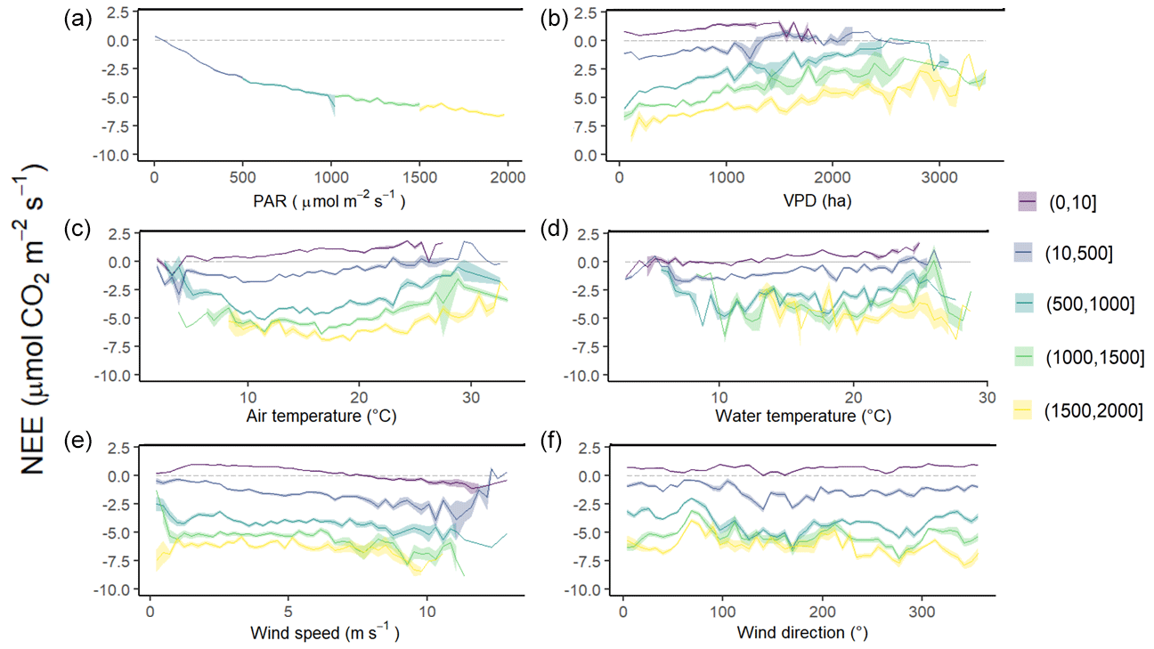
Figure 6 Diurnal variations of NEE fluxes (µmol CO₂ m⁻² s⁻¹) measured every 10 min according to different variables within five PAR groups: 0–10 (night-time), 10–500, 500–1000, 1000–1500 and 1500–2000 µmol m⁻² s⁻¹. Panel (a) shows PAR (µmol m⁻² s⁻¹), (b) VPD (Pa), (c) air temperature (°C), (d) water temperature (°C), (e) wind speed (m s⁻¹) and (f) wind direction (°). NEE fluxes are averaged after separating each variable into five classes and the coloured area is the standard error at the mean.

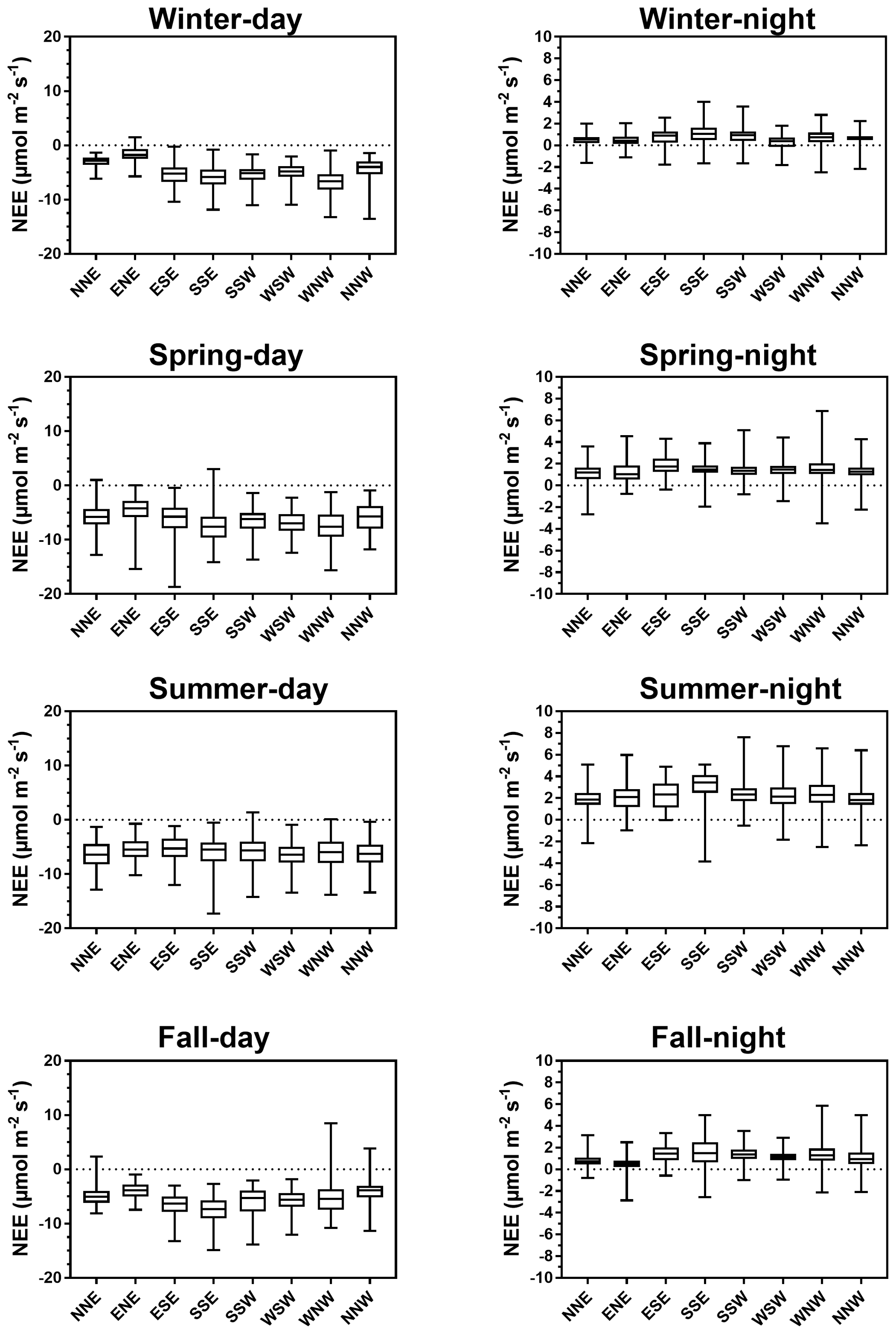
Figure 7 Spatial split of NEE fluxes (µmol CO₂ m⁻² s⁻¹) within each 45° wind sector (Fig. 2) during emersion periods (H_w = 0 m) at the seasonal and diurnal scales. During daytime, the brightest emersion periods (PAR ≥ 500 µmol m⁻² s⁻¹) were chosen to reduce NEE fluctuations due to PAR influence (see Fig. 6a).

3.4 Influence of environmental drivers on temporal NEE variations

Throughout the year, NEE fluxes were significantly controlled by solar radiations and air temperatures at the multiple timescales studied, thereby favouring marsh CO₂ uptake. During daytime (PAR > 10 µmol m⁻² s⁻¹), PAR and T_a displayed the strongest negative correlations with NEE at both the monthly scale (−0.87 and −0.65, respectively; n = 12, p < 0.05) and the 10 min scale (−0.77 and −0.21, respectively; n = 27 160, p < 0.05). The highest and lowest correlations between NEE and PAR were recorded for 10 < PAR ≤ 500 and for 1500 < PAR ≤ 2000 µmol m⁻² s⁻¹, respectively, confirming the rapid increase or decrease in CO₂ uptake for low daytime PAR values (Fig. 6a). During daytime, vapour pressure deficit (VPD) was negatively correlated with NEE (−0.31; n = 27 160, p < 0.05) producing a large reduction in CO₂ uptake for all PAR levels and even led to a switch from sink to source of atmospheric CO₂ from VPD > 1200 Pa for low PAR levels (PAR ≤ 500 µmol m⁻² s⁻¹; Fig. 6b). During night-time and daytime, air temperature (T_a) was positively (0.54; n = 27 190, p < 0.05) and negatively (−0.21; n = 25 544, p < 0.05) correlated with NEE, respectively. However, from PAR > 500 µmol m⁻² s⁻¹, high T_a values (> 20 °C) decreased CO₂ uptake for all PAR levels (Fig. 6c). Water temperature (T_w) did not influence NEE during immersion (Fig. 6d). Indeed, for PAR > 500 µmol m⁻² s⁻¹ and H_w > 0.5 m, no significant relationship was found between NEE and T_w (n = 1215; p = 0.26). For low PAR levels (PAR ≤ 500 µmol m⁻² s⁻¹), wind speeds quickly increased CO₂ uptake, whereas for high PAR levels (PAR > 500 µmol m⁻² s⁻¹), CO₂ uptake was increased only for wind speeds higher than 7 m s⁻¹ (Fig. 6e). For wind directions, a spatial heterogeneity of NEE was recorded according to wind sectors both during daytime and night-time (Fig. 6f). Within the footprint area composed of an assemblage of plants and muds (Fig. 2), the highest CO₂ uptakes were generally recorded from the southern sectors (high vegetation:mud ratios) whereas, the lowest CO₂ uptakes were generally recorded from the northern sectors (low vegetation:mud ratios; Fig. 7). For instance, our sectorial NEE analysis during daytime emersion showed that the SSE sector (vegetation:mud ratio of 2.4; Table 1) did uptake 32 % (winter), 25 % (spring) and 50 % (fall) times more atmospheric CO₂ than the NNW sector (vegetation:mud ratio of 0.8; Table 1). Moreover, in winter and fall, we highlighted that CO₂ uptake rates of H. portulacoides (C₃ species) were significantly higher than S. maritima (C₄ species) ones by comparing the SSE (60 % of H. portulacoides and 9 % of S. maritima) and WSW (33 % of H. portulacoides and 35 % of S. maritima) sectors during daytime emersion (Mann–Whitney tests, p < 0.0001). In contrast, in summer, no significant difference in NEE fluxes was recorded between these two sectors (Mann–Whitney test, p = 0.06; Fig. 7) and, more generally, between the different wind sectors (Fig. 7; Table 1). For all seasons, during night-time emersion, we recorded that southern sectors (ESE, SSE and SSW) emitted higher atmospheric CO₂ than northern sectors (NNE and ENE), especially in winter and fall (Fig. 7; Table 1).

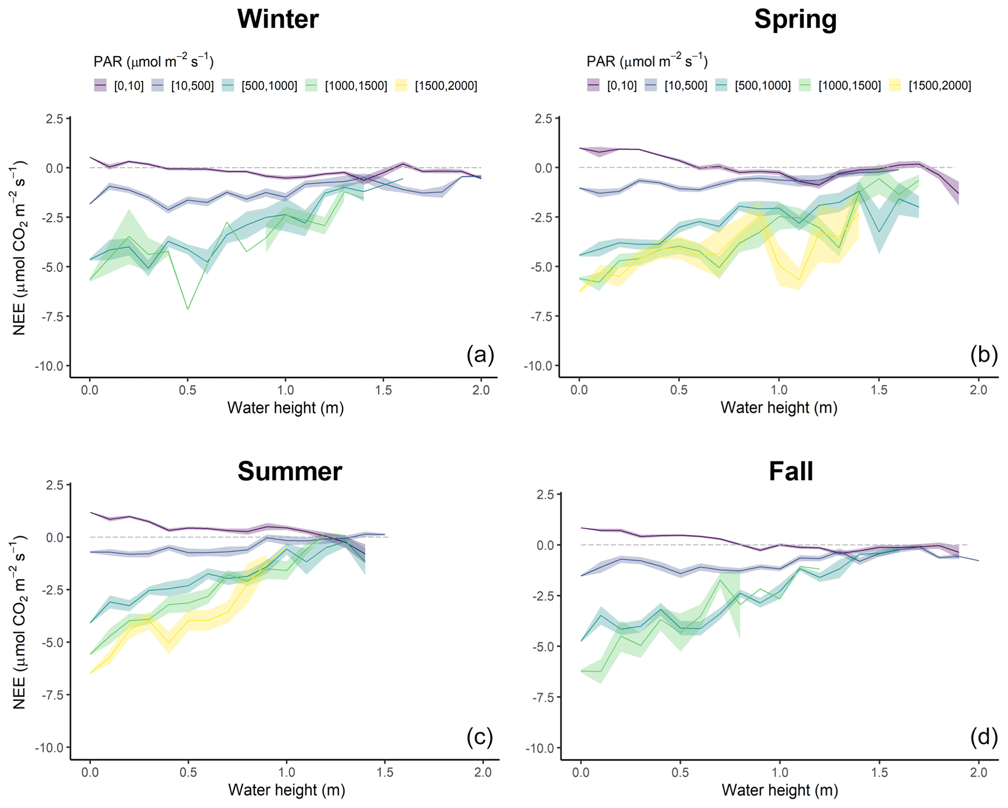
Figure 8 Diurnal variations of NEE fluxes (µmol CO₂ m⁻² s⁻¹) measured every 10 min according to water height (H_w, m) within five PAR groups (see caption of Fig. 6) in winter (a), spring (b), summer (c) and fall (d). NEE values were averaged every 0.1 m. The coloured areas represent the standard error of the mean.

The tidal rhythm strongly influenced NEE fluxes during immersion depending on water heights (H_w) and PAR levels (Figs. 8 and S3). Throughout the year, NEE were positively correlated with H_w during the day but negatively correlated during the night (Fig. 8). More precisely, night-time immersion strongly reduced CO₂ emissions and even led to a switch from source to sink of atmospheric CO₂ from H_w > 0.4 m in winter (Fig. 8a), H_w > 0.7 m in spring (Fig. 8b), H_w > 1.4 m in summer (Fig. 8c) and H_w > 1 m in fall (Fig. 8d), on average. For low daytime PAR levels (PAR ≤ 500 µmol m⁻² s⁻¹), immersion only slightly reduced CO₂ uptake (Fig. 8c). On the contrary, for higher daytime PAR levels (PAR > 500 µmol m⁻² s⁻¹), immersion strongly reduced CO₂ uptake, especially from H_w > 0.5 m, to reach the lowest CO₂ sinks from H_w > 1.0 m, irrespective of the PAR levels (Fig. 8c).

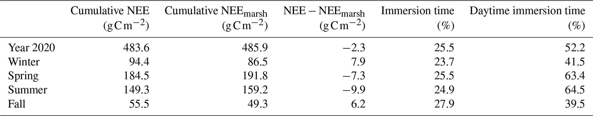
Table 4 Net seasonal carbon balances for the measured NEE and estimated NEE_marsh values (g C m⁻²). Corresponding seasonal percentages of marsh immersion and daytime marsh immersion are indicated. NEE corresponds to net vertical CO₂ exchanges measured by EC, whereas NEE_marsh corresponds to net vertical CO₂ exchanges estimated at the benthic interface without any tidal influence.

3.5 Annual carbon budgets

Throughout the year, the annual NEE value was −483.6 $\mathrm{g}\mathrm{C}{\mathrm{m}}^{-\mathrm{2}}{\mathrm{yr}}^{-\mathrm{1}}$, associated with immersion duration of 6.1 h d⁻¹, on average. Simultaneously, estimated GPP and R_eco (marsh metabolic fluxes without tidal influence) absorbed and emitted 1019.4 and 533.2 $\mathrm{g}\mathrm{C}{\mathrm{m}}^{-\mathrm{2}}{\mathrm{yr}}^{-\mathrm{1}}$, respectively, resulting in an annual estimated NEE_marsh value similar to the measured NEE value (Fig. 9). At the seasonal scale, the highest CO₂ uptakes occurred in spring and summer, associated with the lowest marsh immersion levels, and the lowest CO₂ uptakes occurred in winter and fall, associated with the highest marsh immersion levels (Tables 2 and 4). In winter and fall, when the daytime immersion periods were the shortest, net C balances from measured NEE gave higher values than net C balances from estimated NEE_marsh (+7.9 and +6.2 g C m⁻², respectively; Table 4). Conversely, in spring and summer when the daytime immersion periods were the longest, the opposite pattern was observed between measured NEE values and estimated NEE_marsh values (−7.3 and −9.9 g C m⁻², respectively; Table 4).

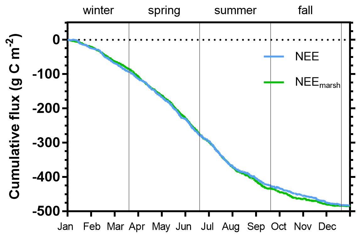
Figure 9 Cumulative carbon fluxes (g C m⁻²) of the measured NEE (in blue) and estimated NEE_marsh (in green) throughout the year 2020. Vertical lines are used to delimit the four seasons. NEE fluxes correspond to net vertical CO₂ exchanges measured by EC, whereas NEE_marsh fluxes correspond to net vertical CO₂ exchanges estimated from NEE partitioning at the benthic interface only, without any tidal influence.

4 Discussion

4.1 Marsh CO₂ uptake and influence of management practice

In the present EC study, the salt marsh absorbed 483 $\mathrm{g}\mathrm{C}{\mathrm{m}}^{-\mathrm{2}}{\mathrm{yr}}^{-\mathrm{1}}$ from the atmosphere. This net C balance (i.e. budget) was lower than the values estimated for global tidal wetlands (1125 $\mathrm{g}\mathrm{C}{\mathrm{m}}^{-\mathrm{2}}{\mathrm{yr}}^{-\mathrm{1}}$; Bauer et al., 2013) and for tidal marshes on the Atlantic coast of the United States (775 $\mathrm{g}\mathrm{C}{\mathrm{m}}^{-\mathrm{2}}{\mathrm{yr}}^{-\mathrm{1}}$; Wang et al., 2016) but similar to the C balance estimated by Alongi (2020) for global salt marshes (382 $\mathrm{g}\mathrm{C}{\mathrm{m}}^{-\mathrm{2}}{\mathrm{yr}}^{-\mathrm{1}}$).

Table 5 Comparison of the annual NEE budget ($\mathrm{g}\mathrm{C}{\mathrm{m}}^{-\mathrm{2}}{\mathrm{yr}}^{-\mathrm{1}}$) using EC measurements across the salt, brackish and freshwater marshes of the coastal zone.

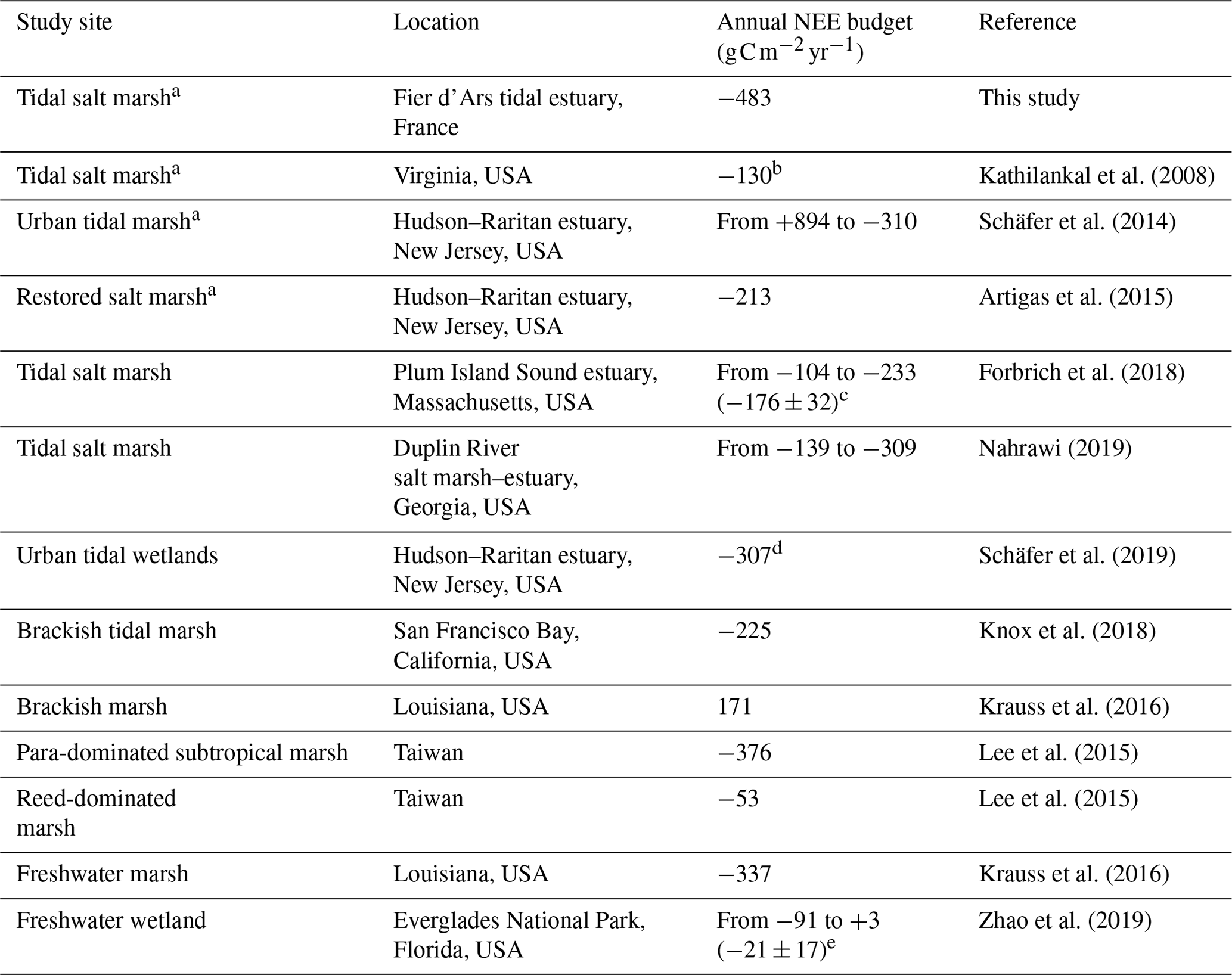
^a Managed and protected marshes. ^b NEE budget during the growing season (from May to October 2007). ^c Mean of annual NEE budgets over a 5-year period (from 2013 to 2017). ^d Annual NEE budget of three tidal marshes with different restoration histories. ^e Mean of annual NEE budgets over a 9-year period (from 2008 to 2016).

Currently, an increasing number of EC measurements are being taken in salt marshes in order to obtain continuous NEE data series as well as to increase knowledge about the associated metabolic processes and fluxes for these tidal systems (Table 5) (Schäfer et al., 2014; Forbrich et al., 2018; Knox et al., 2018). These EC studies confirmed the estimates of CO₂ sinks in salt marshes (Wang et al., 2016; Alongi, 2020) but also revealed strong NEE flux heterogeneities according to climatic conditions and anthropogenic influences (Herbst et al., 2013; Schäfer et al., 2019). For instance, NEE measured in a natural salt marsh (S. alterniflora, S. maritima and D. spicata) showed a net C uptake from the atmosphere with high interannual variations in C balances (Table 5) mainly due to rainfall during the growing season for marsh plants (Forbrich et al., 2018). By comparison, in an urban tidal marsh, Schäfer et al. (2014) reported a higher interannual variability from 984 g C m⁻² in 2009 to −310 g C m⁻² in 2012 due to management practices and plant species (P. australis and S. alterniflora in 2009 and total elimination of P. australis in 2012; Table 5). In the same area, in another restored salt marsh in which the P. australis monoculture was replaced by a high diversity of emergent marsh plants (S. patens, S. cynosuroides, S. alterniflora and D. spicata), a net CO₂ uptake was recorded (Table 5) which once again confirms the importance of land management practices in marsh C balances (Artigas et al., 2015). In our studied salt marsh, the natural management for several decades has allowed for a return to the natural site hydrodynamics and the development of productive marsh halophytes, mainly composed of H. portulacoides and S. maritima (59 % of the footprint area). However, past human activities and water management practices for salt farming have shaped the marsh typology (channel network, humps and dykes), producing a time-delayed immersion of plants and muds between high and low marsh areas during spring tides. Thus, due to this emersion/immersion heterogeneity, mud and S. maritima were quickly immersed by coastal waters, whereas the whole immersion of marsh habitats only occurred during the highest tidal amplitudes favouring a higher atmospheric CO₂ uptake by H. portulacoides and S. vera. During the year 2020, our rewilded salt marsh took up more C from the atmosphere mainly due to strong plant photosynthesis than the other salt, brackish and freshwater marshes reported in the literature (Table 5). However, the net C balances calculated with the EC method are still too scarce to be able to take all temporal and spatial variabilities of salt marshes into account. Based on biomass production measurements in salt marshes, Sousa et al. (2010) estimated that the NPP of H. portulacoides was 505 $\mathrm{g}\mathrm{C}{\mathrm{m}}^{-\mathrm{2}}{\mathrm{yr}}^{-\mathrm{1}}$, whereas the NPP of S. maritima varied between 367 and 959 $\mathrm{g}\mathrm{C}{\mathrm{m}}^{-\mathrm{2}}{\mathrm{yr}}^{-\mathrm{1}}$ depending on the chemical–physical characteristics and marsh maturity. Thus, the net metabolism of these halophytic plants could play an important role in our net C balance but, according to “the marsh CO₂ pump” (Wang et al., 2016), a significant proportion of marsh NPP was respirated by heterotrophic processes and then (1) emitted as atmospheric CO₂ (38 ± 11 %) and (2) exported by tides as DIC (37 ± 15 %; Song et al., 2023).

Moreover, despite a lower benthic metabolism (photosynthesis and respiration) of muds than evergreen plants (Fig. 7), the microphytobenthos which can develop on mudflats (27 % of the footprint area) may also contribute to marsh production during daytime emersion, as highlighted in our studied marsh where static chamber measurements performed in March 2023 at midday showed a net CO₂ uptake to a non-vegetated mudflat (NEE mean of −2.92 µmol m⁻² s⁻¹; unpublished results) and confirmed in an estuarine wetland in China (Xi et al., 2019). On an intertidal flat (France), EC measurements even showed a higher daily benthic metabolism with microphytobenthos (1.72 $\mathrm{g}\mathrm{C}{\mathrm{m}}^{-\mathrm{2}}{\mathrm{d}}^{-\mathrm{1}}$; September/October 2007) than with Zostera noltei (1.25 $\mathrm{g}\mathrm{C}{\mathrm{m}}^{-\mathrm{2}}{\mathrm{d}}^{-\mathrm{1}}$; July and September 2008), confirming the high biological productivity of mudflats (Polsenaere et al., 2012). However, due to the specific assemblage of our studied marsh (Fig. 2), it remains complex to accurately study these habitat effects (plants vs. microphytobenthos) on NEE fluxes at the marsh scale and draw more general conclusions. Thus, the microphytobenthos could play a significant role in the atmospheric CO₂ uptake of salt marshes but also, more generally, in the carbon cycle of the coastal ocean because the resuspension of the microphytobenthos primary production during tidal immersion induce a large export of organic carbon from muds to coastal waters (up to 60 % of the benthic primary production in a nearby tidal flat; Savelli et al., 2019). These fast-growing primary producers with high labile organic carbon could also be quickly degraded locally by microbial remineralization (Ruttenberg, 1992; De Brouwer and Stal, 2001; Morelle et al., 2022), contrary to evergreen plants contributing to long-term “blue carbon” burial in sediments (Mcleod et al., 2011).

4.2 Metabolism processes and controlling factors at multiple timescales

4.2.1 Seasonal scale

In a tidal salt marsh, the average monthly budgets from Forbrich et al. (2018) showed a net CO₂ sink during the growing season for marsh plants from June to September and a net CO₂ source to the atmosphere during the rest of the year, indicating a strong seasonal variability in marsh metabolic fluxes. In urban salt marshes, the growing season was longer switching from source to sink in May (Schäfer et al., 2014; Artigas et al., 2015) and even in April in a brackish marsh (Knox et al., 2018). In our studied marsh, the halophyte vegetation, mostly composed of evergreen species, was autotrophic throughout the year allowing a net C uptake from the atmosphere during both the growing and non-growing seasons (between 9 g C m⁻² in December and 73 g C m⁻² in July), whereas the senescence of smooth cordgrass plants in some salt marshes (S. alterniflora and S. cynosuroides, for instance) from October produced a marsh heterotrophy and a net C source to the atmosphere in winter and fall (Schäfer et al., 2014; Artigas et al. 2015; Forbrich et al., 2018). In our case, S. maritima is a perennial species with a relatively short growing period. Indeed, during winter and fall, the metabolism of this halophytic plant could have a significantly lower influence on marsh C uptake than H. portulacoides and S. vera. The spatial NEE analysis showed that, in summer during daytime emersion, CO₂ uptake rates of the northern sectors (high mudflats areas) were close to ones of the southern sectors (high plants areas) which suggests a low heterotrophic respiration in the mudflats during this period. The low R_eco rates related to plant and soil respiration processes resulted in lower atmospheric CO₂ emissions in the studied salt marsh than in urban salt marshes (Artigas et al., 2015) and brackish marshes (Knox et al., 2018), thus allowing a net CO₂ sink from winter to summer. Moreover, our low R_eco is also likely linked to the low OM decomposition observed at our site, notably due to recalcitrant OM (Arnaud et al., 2024). Furthermore, it is also important to better understand the direct and indirect effects of meteorological conditions and tidal immersion on photosynthesis and respiration processes and the associated marsh C balances (Knox et al., 2018).

Our study showed the predominant role of PAR and T_a on NEE variations in the salt marsh as has already been highlighted elsewhere by Wei et al. (2020b). Our correct NEE flux partitioning into GPP and R_eco during emersion indicated that plant photosynthesis was mainly driven by light, while ecosystem respiration was mainly driven by temperature. At the seasonal scale, the strongest CO₂ sinks were measured during warm and bright periods such as spring and summer, which were responsible for 70 % of the annual C uptake (Table 4). However, although the highest seasonal rate of GPP was measured in summer during the brightest months, the simultaneously recorded high T_a values instead favoured ecosystem respiration producing a lower net CO₂ uptake in summer than in spring (Table 4). For instance, in two urban salt marshes, the T_a values above 30 °C reduced CO₂ uptake by increasing respiration and atmospheric CO₂ emissions (Schäfer et al., 2019). These two meteorological parameters controlled short- and long-term NEE variations, as confirmed in urban salt marshes where significant and strong pairwise correlations of NEE with net radiation and temperature were recorded on half hourly, daily and monthly averages (Schäfer et al., 2019).

At the studied salt marsh, we showed a significant influence of VPD and RH on daytime NEE variations favouring plant CO₂ uptake for the lowest VPD values (< 1000 Pa) and the highest RH values (> 80 %). The lack of a significant relationship between NEE and RH at night indicated that humidity influenced plant photosynthesis, by decreasing VPD and stomata opening, rather than their respiration. In a similar tidal salt marsh, Forbrich et al. (2018) showed a link between rainfall and C budgets on interannual variations in NEE, i.e. during the early growing season in spring, rainfall events produced a decrease in soil salinity and favoured CO₂ uptake through an increase in plant productivity. In a salt marsh in the Yellow River Delta, significant NEE increases and GPP decreases were recorded with high soil salinities during emersion using static chamber measurements (Wei et al., 2020a). High levels of soil salinity in salt marshes are a stressor for plants such as Spartina spp. and can lead to reduce biomass production by inhibiting nutrient and CO₂ uptake throughout stomatal closure (Morris, 1984; Hwang and Morris, 1994). Thus, in our studied marsh, we believe that the increase in dryness periods, especially in summer, with a decrease in rainfall events could profoundly modify plant productivity and marsh C uptake. This was confirmed by a significant reduction in the CO₂ sink at the studied salt marsh with low RH and high T_a values.

4.2.2 Diurnal and tidal scale influences

High-frequency EC measurements demonstrated that diurnal variations in NEE fluxes were driven by light, rather than air temperature (Xi et al., 2019; Wei et al., 2020b), with no significant time delay recorded between NEE and PAR variations (Fig. S2). At our studied site, the highest negative correlations between NEE and PAR were highlighted for low daytime PAR values, indicating that the increases in light during the morning strongly favoured CO₂ uptake mainly through plant photosynthesis up to the middle of the day. During the afternoon, the high T_a and VPD values (warm and dry periods) produced a reduction in photosynthetic rates through stomatal closure of the C₃ plants (Lasslop et al., 2010). This GPP decrease associated with a R_eco increase in afternoon reduced the net CO₂ uptake up to reach CO₂ emissions during night-time (Knox et al., 2018; Xi et al., 2019). In another tidal salt marsh, Kathilankal et al. (2008) confirmed the PAR importance on Spartina photosynthesis and diurnal NEE fluxes. In a restored salt marsh, EC measurements also showed that the time of day has a major influence on atmospheric CO₂ exchanges during the growing season, accounting for 49 % of NEE variability (Artigas et al., 2015). Moreover, in some cases, soil respiration can also be controlled by PAR or photosynthesis at the diurnal scale (Vargas et al., 2011; Jia et al., 2018; Mitra et al., 2019), once again highlighting the major role played by light in diurnal NEE variations (Kathilankal et al., 2008; Wei et al., 2020b). In winter, negative NEE fluxes were measured during some night-time emersion periods in the absence of any photosynthetic processes (18.5 % in January, 18.1 % in February and 10.7 % in March). These negative fluxes could have two main sources: (1) an inorganic CO₂ diffusion and dissolution processes in saline/alkaline soils over mudflats (Ma et al., 2013) and (2) an inflow of coastal waters undersaturated in CO₂ with respect to the atmosphere within the footprint area (in channel; Fig. 2) but not seen by the STPS probe due to our one-location water height measurement and immersion marsh heterogeneity (see Sect. 2.2). The negative values during night-time emersion could reduce the night-time random forest model performance for EC data gap-filling and produce an underestimation of respiration coefficients for NEE flux partitioning (particularly b) even causing a negative coefficient (February; Table S2).

At the daily scale, the intensity of atmospheric CO₂ exchanges and the metabolic status of the marsh (sink/source) were also significantly influenced by the tidal rhythm (Fig. 8). Tides produced a significant decrease in daytime CO₂ uptake with maximal reductions up to 90 % for the highest tidal amplitudes. In a S. alterniflora salt marsh, a mean reduction of 46 ± 26 % was measured during immersion, although large CO₂ amounts were still assimilated at a reduced rate (Kathilankal et al., 2008). In some cases, daytime NEE fluxes could be completely suppressed during immersion in salt marshes (Moffett et al., 2010; Forbrich and Giblin, 2015; Wei et al., 2020a) and brackish marshes (Knox et al., 2018). This drop in CO₂ uptake could be related to a physiological stress for plants under tidal immersion conditions resulting in a reduction in the effective photosynthetic leaf area and photosynthesis rates (Kathilankal et al., 2008; Moffett et al., 2010). Moreover, the physical barrier created by tidal waters could limit the CO₂ diffusion from waters to plants, thereby resulting in fewer CO₂ exchanges between the atmosphere and the benthic compartment (sediments and soil). Using chamber measurements at different tidal stages, Wei et al. (2020a) also highlighted the importance of water heights and marsh immersion levels in NEE variations and confirmed a significant GPP decrease during immersion. However, tidal effects on daytime NEE fluxes may be more variable depending on the immersion level of the marsh and the biogeochemistry state of the tidal waters. Indeed, during the brightest periods in winter and spring, the temporary increases in CO₂ uptake recorded during incoming tides could be related to (1) an increase in the GPP of H. portulacoides and S. vera (highest marsh levels) favoured by VPD and T_a decreases due to tidal conditions and/or (2) tidal waters advected from the shelf that are undersaturated in CO₂ with respect to the atmosphere due to phytoplankton blooms (Mayen et al., 2024). Moreover, when the salt marsh was fully immersed at high tide during spring tides, NEE fluxes were mostly controlled by ecosystem respiration and/or inorganic processes (carbonate and physicochemical pumps) rather than by photosynthesis, as light was no longer a major controlling factor for CO₂ uptake in tidal waters.

During night-time, CO₂ emissions from the salt marsh were inhibited by tidal effects through a significant decrease in ecosystem respiration (Han et al., 2015; Knox et al., 2018; Wei et al., 2020a). The physical barrier formed by tidal waters limits the atmospheric CO₂ releases via respiration from plants and soils (Wei et al., 2020b). Moreover, saturation of surface soils in tidal waters during immersion could reduce oxygen availability in the soil and limit OM microbial decomposition and CO₂ emissions through aerobic respiration (Nyman and DeLaune, 1991; Miller et al., 2001; Jimenez et al., 2012; Han et al., 2015). In our case, night-time CO₂ exchanges were reduced up to 100 % (completely suppressed), sometimes even causing a change in metabolic status of atmospheric CO₂ from source to sink, especially in winter when the R_eco rates were the lowest. The presence of tidal waters advected from the shelf during the night, and CO₂ undersaturated with respect to the atmosphere due to previous phytoplankton production and/or CaCO₂ dissolution in the water column during the day (Gattuso et al., 1999; Polsenaere et al., 2012), could induce a sink which may lead to a net uptake of CO₂ at night (Fig. 8). The results of our study indicate that tidal NEE variations may be mainly related to the marsh immersion level, the PAR level and the time of the growing cycle of plants as reported in Nahrawi et al. (2020).

4.3 Salt marsh carbon budgets for future research perspectives

At the annual scale in 2020, the tidal rhythm did not significantly affect the net C balance of the studied salt marsh since similar annual measured NEE and estimated NEE_marsh values were recorded (Fig. 9). The loss of CO₂ uptake measured during daytime immersion due to a GPP decrease could be compensated by night-time immersion where CO₂ emissions and R_eco were inhibited. However, strong temporal variabilities were measured, especially between the growing and non-growing seasons. In winter and fall, the salt marsh did uptake more C from the atmosphere with the tidal influence (measured NEE) than without (estimated NEE_marsh), especially in December (+35.7 %), November (+19.7 %) and January (+15.4 %), associated with the highest photosynthetic efficiencies. An opposite trend was observed in spring and summer with a reduction in net C uptake under tidal influence, especially in August (−16.9 %) and September (−9.8 %). This significant difference in the seasonal C balances could be mainly related to the photoperiod of immersion periods. We demonstrated that daytime immersion decreased CO₂ uptake, whereas night-time immersion decreased CO₂ emissions up to a change in metabolic status for the highest immersion levels. Thus, during seasons where daytime immersion primarily occurs, such as spring and summer, the salt marsh did uptake less atmospheric CO₂ with tidal influence, whereas seasons that mostly have night-time immersion did uptake more atmospheric CO₂ with tidal influence (Table 4). However, this unpublished result was only possible provided that the salt marsh switched from a source to a sink of CO₂ during night-time immersion due to water undersaturation with respect to the atmosphere. In a salt marsh on Sapelo Island (USA), Nahrawi et al. (2020) highlighted tidal CO₂ flux reductions all year round by distinguishing neap tide and spring tide periods. Their results showed that the highest and lowest reductions in C uptake occurred in spring (−34 %) and summer (−13 %), respectively, with a similar but greater tidal influence on the C uptake values compared with our study.

To better constrain the tidal influence on the metabolism of the salt marsh, further investigations have been carried out in 2021 in parallel with our EC measurements, with the construction of a digital field model for water heights that can be used to spatially determine, over the whole EC footprint, the exact areas of immersion and emersion (especially for the low water levels) of the marsh in each sector at a 10 min step. Similarly, during marsh immersion, EC measurements do not directly capture CO₂ fluxes from benthic metabolism because of the physical barrier of the water and the lower CO₂ diffusion rates in water than in air. Consequently, at the same time as when the NEE measurements were taken, water pCO₂, inorganic and organic carbon concentrations associated with planktonic metabolism were determined each season through 24 h cycles to provide essential information on the contribution of planktonic communities and plants to CO₂ fluxes during immersion (Mayen et al., 2024). The lateral carbon export from salt marshes by tides plays a significant role in the coastal ocean carbon cycle (Guo et al., 2009; Wang et al., 2016). Plant respiration and microbial mineralization of marsh NPP could generate Dissolved Inorganic Carbon (DIC) in waters associated with a strong benthic–pelagic coupling. Thus, our 2021 measurements of the carbon parameters, planktonic metabolism (production and respiration) and other relevant biogeochemical variables over 24 h diurnal cycles, along with measurements of the soil compartment (root OM production vs. mineralization; Arnaud et al., 2024) carried out in the EC footprint, would allow for a more integrative calculation of the studied marsh carbon budget (Mayen et al., 2024). One advantage of the EC measurements is the aggregation of CO₂ fluxes from all compartments (waterbodies, soil, plants and atmosphere) in salt marshes. Yet, through this flux aggregation, we cannot mechanistically understand each marsh compartment, and therefore it can be challenging to predict CO₂ fluxes under multiple global changes. Therefore, future contributions should try to simultaneously quantify all these compartments, especially soil as it is where most of the carbon is stored in salt marshes (Arnaud et al., 2024). Ongoing atmospheric CO₂ exchange measurements are actually carried out since January 2023 up north over Aiguillon (intertidal) Bay in France where we precisely deployed an EC station at the edge between the tidal mud flat on the west side and salt marsh habitats on the east side of the footprint along with benthic chamber flux and water, sediment, soil carbon measurements and satellite analysis at each season to specially address questions on relative habitat (mudflat vs. salt marshes) influence on atmospheric CO₂ exchanges (Pierre Polsenaere, personal communication, 2023).

5 Conclusion

In this study, we used the micrometeorological eddy covariance technique to investigate the net ecosystem CO₂ exchanges (NEE) at different timescales and to determine the major biophysical drivers of a rewilded tidal salt marsh. During the year 2020, the net C uptake from the atmosphere (−483 $\mathrm{g}\mathrm{C}{\mathrm{m}}^{-\mathrm{2}}{\mathrm{yr}}^{-\mathrm{1}}$) was mainly related to a low OM decomposition rate coupled with an intense autotrophic metabolism of halophyte plants, especially during the growing season, driven by light, temperature and VPD. In summer, the brightest days increased the plant GPP and, simultaneously, high temperature and VPD values favoured R_eco resulting in a lower net CO₂ uptake in summer than in spring. At the daily scale, the tidal rhythm significantly influenced NEE fluxes according to the level of marsh immersion and PAR. During daytime, tides strongly limited atmospheric CO₂ uptake, up to 90 % reductions, whereas night-time immersion inhibited atmospheric CO₂ emissions through plant and soil respiration, sometimes even causing a change in metabolic status from source to sink. However, at the annual scale, NEE flux partitioning into NEE_marsh highlighted that the tidal rhythm did not significantly affect the net marsh C balance. Our continuous NEE measurements have made it possible to better understand the biogeochemical functioning of salt marshes over a wide range of environmental conditions and have provided essential information on NEE fluxes in marshes undergoing potential future changes such as global warming or sea level rise.