Selecting allometric equations to estimate forest biomass from plot- rather than individual-level predictive performance

In the context of global change, it is essential to quantify and monitor the carbon stored in forests. Allometric equations are mathematical models that predict the biomass of a tree from dendrometrical characteristics that are easier to measure, such as tree diameter, height, or wood density. Various model forms have been proposed for allometric equations. Moreover, the model choice has a critical influence on the estimate of the biomass of a forest. So far, model selection for allometric equations has been performed based on the tree-level predictive performance of the models. However, allometric equations are used to estimate the biomass of plots rather than individual trees. The distribution of trees sampled for establishing allometric equations often differs from the forest structure. Moreover, at the plot level, the residual individual errors for different trees can cancel off. Therefore, we expect the plot-level predictive performance of a model to differ from its tree-level performance. Using a dataset giving the observed biomass of 844 trees in central Africa and a null model for the size distribution of trees in the forest, we simulated forest plots between 0.1 and 50 ha in area. Then, using a Monte Carlo approach, we calculated the mean sum of squared errors (MSS) of the differences between observed and predicted plot biomass. We showed that MSS could be well approximated by a three-term formula, where the first term corresponded to bias, the second one corresponded to the tree residual error, and the third one corresponded to the uncertainty on model coefficients. For small plots (≤ 0.1 ha), the plot-level predictive performance was dominated by the tree residual error term. Model selection based on plot-level predictive performance was then consistent with that based on tree-level performance. For large plots, this term vanished. Model selection based on plot-level performance could then differ from that based on tree-level performance. In the case of large plots, chains of models that combined a general equation to predict biomass and local equations to predict some of the predictors of the biomass equation could provide a good trade-off between the bias in and the uncertainty on model coefficients. We recommend using plot-level rather than tree-level predictive performance to select allometric equations. The three-term formula that we developed provides an easy way to assess the effect of plot size on model selection and to balance the respective contributions of bias, tree residual error, and the uncertainty on model coefficients.

1 Introduction

In the context of changing climate due to increasing CO₂ atmospheric concentration, it is essential to quantify and monitor the main compartments that store or emit carbon at the global level. Forests are one of these compartments and are part of the solution to mitigate climate change (Lewis et al., 2019). However, there are still uncertainties in the quantification of forest carbon stocks, in particular in the tropics (Rodda et al., 2024). Measuring and monitoring forest carbon stocks involves a chain of measurements that starts with biomass measurement at individual tree level and ends with remote sensing techniques (Gibbs et al., 2007; Réjou-Méchain et al., 2019). Typically, tree-level biomass measurements are used to fit allometric equations that predict the biomass of a tree from tree dendrometrical characteristics that are easier to measure, such as diameter, height, or wood density (Chave et al., 2014). Allometric equations are used in turn to estimate the biomass of forest plots. Plot-level biomass can be used to fit plot-level models that predict plot biomass from plot volume and other plot characteristics, using biomass expansion factors or related approaches (Pan et al., 2004; Fang et al., 2007; Guo et al., 2010). These plot-level models can then be used to estimate forest biomass at the country (Fang et al., 2007) and continental (Fang et al., 2014) scales. Plot-level biomass data can also be used to calibrate remote sensing indices to predict the biomass of pixels in satellite images. Satellite images are finally used to map forest biomass on large areas.

Because plot-level biomass data are key for large-scale biomass estimation, it has been proposed to directly measure biomass at the plot level (Clark and Kellner, 2012). Fast-developing measurement techniques like terrestrial or airborne lidar may provide plot-level measures of biomass in the future (Xu et al., 2021). However, based on destructive measurements, plot-level measures of biomass are currently difficult. Allometric equations thus remain an indispensable link in the measurement chain (Vorster et al., 2020). The development of new tree biomass allometric equations is still mobilizing a great deal of scientific effort around the world (Yang et al., 2024). However, the uncertainty on the choice of the allometric equation used to convert inventory data into biomass estimates remains a major source of error (Picard et al., 2016). In this study, we focus on the step of the allometric equation that connects the tree level to the plot level while considering that allometric equations are intended to provide biomass estimates at the plot level rather than at the tree level (McRoberts and Westfall, 2014; McRoberts et al., 2015; Paul et al., 2016).

Improving the predictive performance of allometric equations often consists of reducing their residual standard error. This reduction can be achieved by integrating new predictors into the equation, such as crown dimensions, trunk shape, diameter of the largest branches, or tree architecture (MacFarlane, 2011; Goodman et al., 2014; Brede et al., 2022). New measurement techniques are indeed providing a greater level of detail in the description of trees (Momo Takoudjou et al., 2018; Lines et al., 2022). There is an ecological interest in understanding the drivers of biomass allometry at the tree level (Yang et al., 2024). Nevertheless, the application of allometric equations to plot data over large areas relies on forest inventory data. The use of detailed predictors in allometric equations is thus limited by the set of dendrometrical variables commonly available in forest inventories. In tropical forests, these variables are usually limited to diameter and species. Adding dendrometrical predictors to the model to reduce the tree-level residual error would then inflate the measurement cost to obtain these additional predictors at the plot level.

Beyond the availability of predictors at the plot level, there is a more fundamental reason for not systematically attempting to reduce the residual standard error of allometric equations. A large residual error at the tree level may be compensated at the plot level when the residual errors from different trees cancel off. The leveling off of the individual residual error is all the more important, as the plot is large. Thus, explaining the greatest share of the variance in tree biomass may not always be the best strategy to select an allometric equation to predict plot biomass. Assessing the predictive performance of allometric equations at the plot level, rather than at the individual level, could significantly alter how equations are selected and improved.

Adding a predictor that is not available in inventory data can be achieved by using an auxiliary equation to predict this predictor. Tree height has often been incorporated in biomass allometric equations in this way (Chave et al., 2014). Tree height generally improves the prediction of biomass but is rarely available in large-scale forest inventories. On the other hand, datasets on tree height are much more abundant than datasets on tree biomass, so a diameter–height model can usually be fitted with higher precision than biomass models (Feldpausch et al., 2011). Thus, one option is to predict height from diameter, then biomass from diameter and height, i.e., to use a chain of models (Feldpausch et al., 2012). Another option is to predict biomass from diameter alone. A pending question is which option is the best.

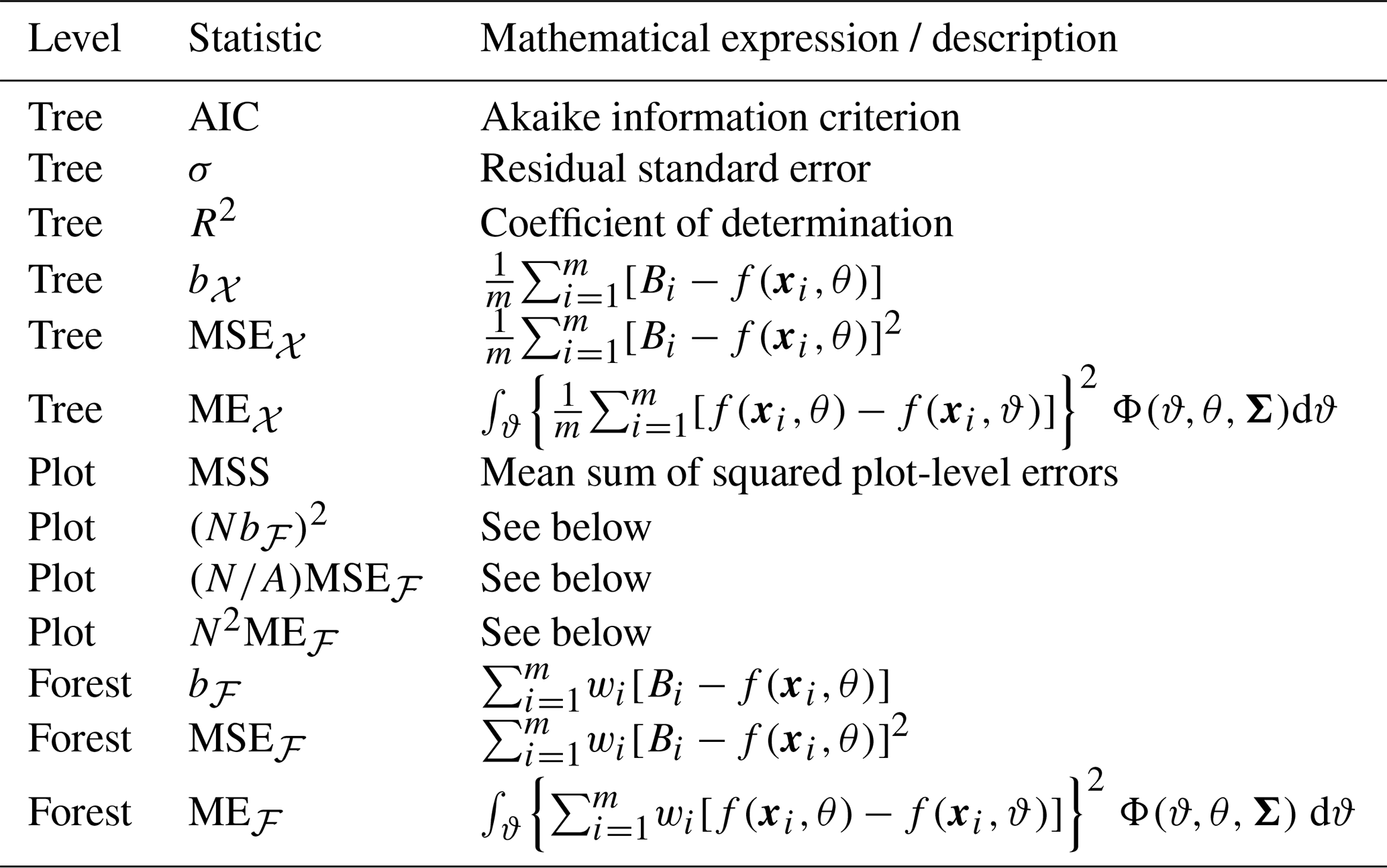
Table 1 Statistics used to assess the predictive performance of a fitted allometric model f at the tree, plot, and forest levels. The mathematical expressions are only specified for the statistics specific to this study. Otherwise, the description of the statistic is recalled. The allometric model f was fitted to a dataset 𝒳 that gave the biomass B_i and the dendrometrical characteristics x_i of m trees. The coefficients θ of model f had a multivariate normal distribution Φ with covariance matrix Σ. A plot with area A and tree density N was obtained by sampling N×A trees from 𝒳 with replacement using the probability of drawing w_i for the ith tree of 𝒳. The forest was the limit when the plot area A tended to infinity for a fixed N.

The objective of this study was to compare allometric equations based on their predictive performance at the plot level rather than at the tree level. We examined whether shifting the focus from the tree to the plot influenced model selection. Different competing models were compared. We placed ourselves in the context of fitting allometric equations, when a calibration dataset of observed tree biomass is available and model coefficients need to be estimated. A different context is when allometric equations are given with known coefficients, and a validation dataset is given to compare their predictive performance. The method we proposed can accommodate models fitted in different ways. It can also be used to assess the predictive performance of a chain of models, i.e., a model that predicts y from x followed by another one that predicts tree biomass from y. Such a situation is often found when it comes to the role of tree height in the prediction of its biomass. Our method is a Monte Carlo method that relied on randomly generated plot-level data, thus allowing us to compare equations for different plot sizes. Given a dataset on individual tree attributes (including tree biomass), a plot was generated by randomly picking trees while constraining plot structural characteristics (such as tree density or basal area) to prescribed values. These plot structural characteristics were set using a null forest model. We used a dataset on tree biomass in the Congo Basin to illustrate the method (Fayolle et al., 2018).

Using this dataset, we addressed the following questions. (i) Does model selection based on predictive performance at tree level agree with model selection based on predictive performance at plot level? (ii) How does plot size affect model selection when this selection is based on predictive performance at plot level? (iii) When extra data on tree height are available so that a height–diameter model can be fitted, does predicted height improve the prediction of biomass through a chain of models? We hypothesized that the role of the residual model error, which is decisive in tree-level predictive performance, decreases with plot size when evaluating plot-level predictive performance.

2 Material and methods

The comparison and selection of allometric equations is commonly based on the goodness of fit of the fitted models, using selection criteria like the Akaike information criterion (AIC), the Bayesian information criterion (BIC), and the root-mean-square error (RMSE). This selection mode puts the emphasis on the predictive performance of the models at the tree level. Here, we assessed the predictive performance of allometric equations (i) at the tree level based on a dataset of tree biomass observations, (ii) at the plot level based on randomly generated plots using a null forest model and the tree dataset, and (iii) at the forest level based on the same null forest model. For each of these three levels, specific performance statistics were used (Table 1).

From a statistical standpoint, criteria like AIC or BIC may be tricky to use to compare models that have been fitted in different ways (e.g., ordinary-least-squares fitting on log-transformed data versus weighted-least-squares fitting on untransformed data). All the models we considered were fitted using linear regression on log-transformed data. Thus, AIC, R², and the residual standard error σ refer to the model fit (i.e., the log-transformed biomass), while the other statistics in Table 1 refer to biomass.

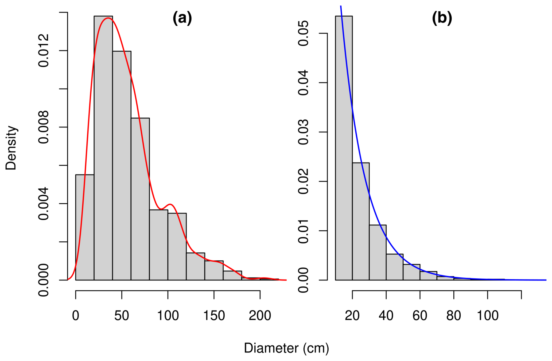
Figure 1 Diameter distribution of (a) the 844 trees sampled in the Congo Basin forests for the measurement of their biomass (Fayolle et al., 2018) and (b) the 10 000 trees resampled from the former set of trees so as to conform to an exponential distribution with parameter 0.0689 cm⁻¹. The red line is a density estimate d_𝒳 of the distribution using a Gaussian kernel with a bandwidth determined by Silverman's rule of thumb. The blue line is the density d_ℱ of the exponential distribution with parameter 0.0689 cm⁻¹. The dataset in panel (b) was obtained from the dataset in panel (a) by resampling each diameter x with a probability proportional to $d_{\mathcal{F}}\left(x\right)/d_{\mathcal{X}}\left(x\right)$.

2.1 Tree biomass data and tree-level predictive performance

We used the dataset on individual tree biomass described in Fayolle et al. (2018). This dataset, denoted 𝒳, includes the diameter, height, wood specific gravity, aboveground biomass, and species of m=844 trees in the Congo Basin. The trees belong to 52 different species and 49 different genera. Data were collected in six countries of the Congo Basin: Cameroon, Central African Republic, Congo, Democratic Republic of the Congo, Equatorial Guinea, and Gabon. Details on tree measurements and data collection are given in Fayolle et al. (2018). Trees in dataset 𝒳 were sampled in the range 10.3–208.0 cm in diameter at breast height (dbh), with a peak of the sampling effort around 35 cm dbh (Fig. 1). Let d_𝒳 be the density of the diameter distribution of trees in dataset 𝒳. This distribution reflects the sampling design of trees and is unrelated to the diameter distribution of trees in the forest.

Let f be an allometric equation that predicts the tree biomass f(x,θ) of each tree using its dendrometrical characteristics x, where θ denotes the coefficients of the model. Model f included the bias correction factor when back-transforming data from the log-transform. A prediction bias remained even with this correction factor. The prediction error for a tree with observed biomass B was $B-f(\mathit{x},\mathit{\theta })$. From the prediction errors for all trees in dataset 𝒳, various performance statistics could be computed, including the prediction bias b_𝒳, which is the average prediction error, and the mean squared error MSE_𝒳 (Table 1). Although rarely considered in the statistics of predictive performance of allometric equations, one may also consider the prediction variability brought by the uncertainty on the model coefficients θ. When using a linear regression to fit the model, the estimator of θ is distributed as a multivariate normal distribution with mean θ and covariance matrix Σ. Drawing coefficient values ϑ according to this multivariate normal distribution, computing the resulting tree biomass f(x,ϑ), and averaging its squared difference with the prediction f(x,θ) brought the mean error ME_𝒳 (Table 1).

As a secondary dataset, denoted 𝒳^′, we used a subset of the pantropical dataset assembled before 𝒳 by Chave et al. (2014). We kept only observations from the Congo Basin (Cameroon, Central African Republic, and Gabon), totaling $m^{\prime }=\mathrm{177}$ trees. The dataset gives the diameter, height, wood specific gravity, and aboveground biomass of trees. However, for the purposes of our study, we only kept the diameter and height variables.

2.2 Null forest stand model and forest-level predictive performance

Plot-level biomass data were generated using the collection of tree biomass measurements and a null model for the diameter structure of the forest. This null model had two entries: the stand density N and its basal area G. Following the hypothesis of demographic equilibrium, the null model assumed that the forest had a reverse-J-shaped diameter distribution that could be modeled by an exponential distribution (Muller-Landau et al., 2006; Picard et al., 2021). The parameter μ of this exponential distribution can be computed from N and G as $\mathit{\mu }=[\sqrt{\mathrm{2}G/\left(\mathit{\pi }N\right)-x_{\mathrm{0}}^{\mathrm{2}}/\mathrm{4}}-x_{\mathrm{0}}/\mathrm{2}{]}^{-\mathrm{1}}$, where x₀ is the minimum diameter for inventory in the forest plot. For N and G we used average values given by Picard et al. (2021), based on sample plots in central Africa: N = 467 ha⁻¹ and G = 29.8 m² ha⁻¹. These values gave μ = 0.0689 cm⁻¹.

An outcome 𝒴 of a plot in the null forest was randomly drawn by resampling dataset 𝒳 so that the diameter distribution of trees in 𝒴 conformed to the exponential distribution with parameter μ. Let $d_{\mathcal{F}}\left(x\right)=\mathit{\mu }\exp [-\mathit{\mu }(x-x_{\mathrm{0}}\left)\right]$ be the density of this target distribution. Because the diameter distribution of trees in 𝒳 differed for the target distribution, the resampling involved unequal weights. Specifically, the ith tree of 𝒳 was resampled with a weight w_i proportional to $d_{\mathcal{F}}\left(x_i\right)/d_{\mathcal{X}}\left(x_i\right)$. In other words,

$$\begin{array}{}\text{(1)}& w_i={\displaystyle \frac{d_{\mathcal{F}}\left(x_i\right)/d_{\mathcal{X}}\left(x_i\right)}{{\sum }_{j=\mathrm{1}}^m{d}_{\mathcal{F}}\left(x_j\right)/d_{\mathcal{X}}\left(x_j\right)}},\end{array}$$

so ${\sum }_{i=\mathrm{1}}^m{w}_i=\mathrm{1}$. For a forest plot with area A, the N×A trees in 𝒴 were thus sampled from 𝒳 with replacement using the probability of drawing w_i for the ith tree of 𝒳.

The forest level was reached by letting the plot area A tend to infinity for a fixed N. In the resulting forest-level distribution of trees, the ith tree of 𝒳 had probability w_i. Replacing equal tree weights $\mathrm{1}/m$ with these unequal weights w_i changed the predictive performance statistics. The prediction bias at the forest level b_ℱ, the mean squared error MSE_ℱ, and the mean error ME_ℱ due to the uncertainty on the model coefficients were thus obtained (Table 1).

2.3 Error partitioning and plot-level predictive performance

The different sources of prediction error at the plot level were assessed using a Monte Carlo approach. Plot variability in biomass predictions was generated by drawing different outcomes of the null forest stand model. The variability due to model coefficients was generated by drawing different outcomes of the model coefficients according to a multivariate normal distribution with mean θ and covariance matrix Σ. Calculations were performed by combining each plot outcome with each coefficient outcome, resulting in a full factorial design.

2.3.1 For a model

Let K be the number of randomly generated forest plots and let J be the number of randomly generated model coefficients. Let n_k be the number of trees in the kth plot, let θ_j be the jth outcome of the model coefficients, and let x_ki and B_ki be the dendrometrical characteristics and observed biomass of the ith tree of the kth plot. Let $e_{kj}=[{\sum }_{i=\mathrm{1}}^{n_k}{B}_{ki}-f({\mathit{x}}_{ki},{\mathit{\theta }}_j\left)\right]/A$ be the difference between the observed biomass of the kth plot and its predicted biomass according to model f using the jth coefficient value per unit of plot area. The plot-level predictive performance of model f was assessed using the mean sum of squares of these differences, denoted mean sum of squared errors (MSS). Using the calculations of the analysis of variance, this mean sum of squared differences could be partitioned into the squared bias, the plot variability, and the coefficient variability (Appendix A1). These three terms could be approximated by (Nb_ℱ)², $(N/A){\text{MSE}}_{\mathcal{F}}$, and N² ME_ℱ, respectively.

2.3.2 For a chain of models

We generalized the assessment of the predictive performance of an equation to a chain of two allometric equations, where the response variable of the first equation is a predictor of the second one. Our computations readily extends to a chain of three or more allometric equations. Let g be an allometric equation that predicts some tree characteristics $\mathit{y}=g(\mathit{x},\mathit{\varphi })$ from some dendrometrical characteristics x of the tree. Let f be a second allometric equation that predicts the tree biomass $f(\mathit{x},\mathit{y},\mathit{\theta })$ using its dendrometrical characteristics x and those predicted by model g. Coefficients θ and ϕ are those of models f and g, respectively. Typically, y is tree height. The chain f∘g cannot be compared to another biomass model using AIC or BIC, whereas the MSS statistic still allowed us to compare their predictive performance.

To the K randomly generated plots and J randomly drawn coefficients θ, we now add L random draws of the coefficients ϕ. Let ϕ_l be the lth outcome of the model coefficients. Let $e_{klj}=\mathit{\{}{\sum }_{i=\mathrm{1}}^{n_k}{B}_{ki}-f[{\mathit{x}}_{ki},g({\mathit{x}}_{ki},{\mathit{\varphi }}_l),{\mathit{\theta }}_j\left]\mathit{\right\}}/A$ be the difference between the observed biomass of the kth plot and its predicted biomass according to the chain f∘g using the jth coefficient value of f and the lth coefficient value of g per unit of plot area. The mean sum of squared errors (MSS) of these differences could be partitioned into four terms (Appendix A2): the squared bias, the plot variability, the variability due to the coefficients of model g, and the variability due to the coefficients of model f.

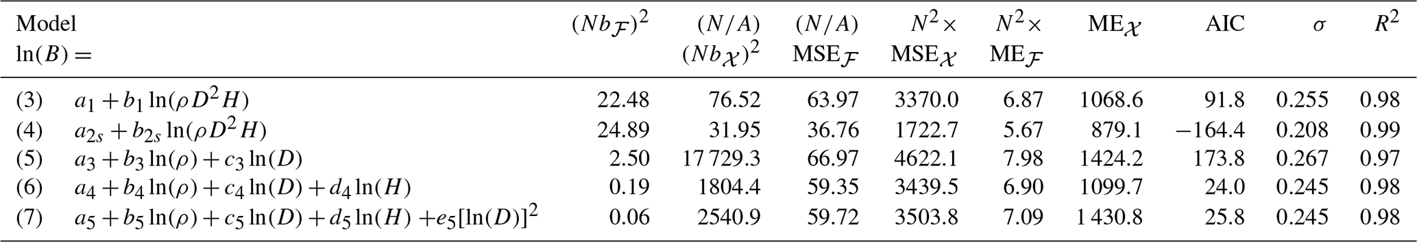
Table 2 Statistics on the predictive performance of five allometric equations fitted to a dataset 𝒳 of 844 trees in the Congo Basin forests. The response variable of all these models is the log-transformed tree aboveground biomass ln (B), with B in kg. ρ is the wood specific gravity in g cm⁻³, D is tree diameter in cm, H is tree height in m, and s denotes the tree genus. N is the density of a forest plot with area A = 1 ha, distributed according to a null forest model ℱ. The quantity b is the prediction biases of tree biomass, MSE is the mean squared error of tree biomass, and ME is the mean error due to coefficient uncertainty. For these three quantities, subscripts ℱ and 𝒳 refer to the null forest and to the fitting dataset. AIC is the Akaike information criterion, σ is the residual standard error, and R² is the coefficient of determination of the fitted model.

2.4 Model comparisons

We compared five allometric equations (see Eqs. 3–7 in Table 2) and one chain of equations. All these models are rooted in the concept of allometry as defined by Huxley and Teissier (1936). It assumes that the relative growth rates of two parts of an individual correlate (Gould, 1966). Models (3) to (6) correspond to simple allometry, where the ratio between relative growth rates is fixed. As discussed by White and Gould (1965), the biologically meaningful parameters are the coefficients associated to covariates. Model (7) corresponds to complex allometry, where the relative growth rate of biomass is a convex function of the relative growth rate of diameter. After back-transformation from the log-transform, model (7) also corresponds to a log-normal model (Picard et al., 2015). Its parameters correspond to maximal biomass, the diameter where biomass reaches its maximum, and a shape parameter. This model can account for senescence: as a tree grows, it accumulates biomass as its diameter increases, until it reaches senescence. When senescent, it may lose biomass (because of dead branches, holes in the trunk, etc.) while its diameter still increases. Regarding the chain of equations, its first model predicted tree height from tree diameter:

$$\begin{array}{}\text{(2)}& \ln \left(H\right)=a_{\mathrm{6}}+b_{\mathrm{6}}\ln \left(D\right),\end{array}$$

while its second model was model (3).

We used F-tests to compare nested models, i.e., to compare models (3) and (4), models (5) and (6), and models (6) and (7). Models (3)–(7) were fitted to dataset 𝒳 with m=844 observations, while model (2) was fitted to $\mathcal{X}\cup {\mathcal{X}}^{\prime }$ with $m+m^{\prime }=\mathrm{1021}$ observations. When back-transforming the data from the log-transform, the bias correction factor $\exp ({\mathit{\sigma }}^{\mathrm{2}}/\mathrm{2})$ was used, where σ was the residual error of the fitted model. Monte Carlo computations were performed with K=1000 and J=1000, bringing 10⁶ values of e_kj. For the chain assessment, we used K=800 and $J=L=\mathrm{50}$, bringing 2×10⁶ values of e_klj. All computations were performed with the software R.

3 Results

The predictive performances of the models differed between the tree level and the forest level. When looking at tree-level performance statistics, the best model was model (4). It had at the same time the lowest AIC, the smallest residual standard error σ, the smallest prediction bias Nb_𝒳, the smallest mean squared error $(N/A){\text{MSE}}_{\mathcal{X}}$, and the smallest mean error due to coefficient uncertainty N² ME_𝒳 among the five competing models (Table 2). When looking at forest-level performance statistics, model (4) still had the smallest mean squared error $(N/A){\text{MSE}}_{\mathcal{F}}$ and the smallest mean error due to coefficient uncertainty N² ME_ℱ among the five models (Table 2). However, it was the worst-performing model in terms of prediction bias Nb_ℱ. The model with the smallest forest-level prediction bias Nb_ℱ was model (7).

The plot-level statistics (Nb_ℱ)², $(N/A){\text{MSE}}_{\mathcal{F}}$, and N² ME_ℱ approximated the terms of the partition of MSS well. The forest-level squared biased (Nb_ℱ)² was a good approximation of the squared bias (SB) component of MSS for plot area greater than 50 ha (Fig. 2c). The SB component of MSS actually showed few fluctuations around (Nb_ℱ)² as the plot area changed (Fig. 2c). The forest-level mean error due to coefficient uncertainty N² ME_ℱ was also a good approximation of the coefficient variability component of MSS for plot area greater than 50 ha (Fig. 2a). Like SB, the coefficient variability showed few fluctuations around N² ME_ℱ as plot area changed (Fig. 2a). In contrast, the plot variability component of MSS sharply decreased with plot area (Fig. 2b). It actually decreased proportionally to the inverse of plot area, with the coefficient of proportionality being well approximated by N MSE_ℱ.

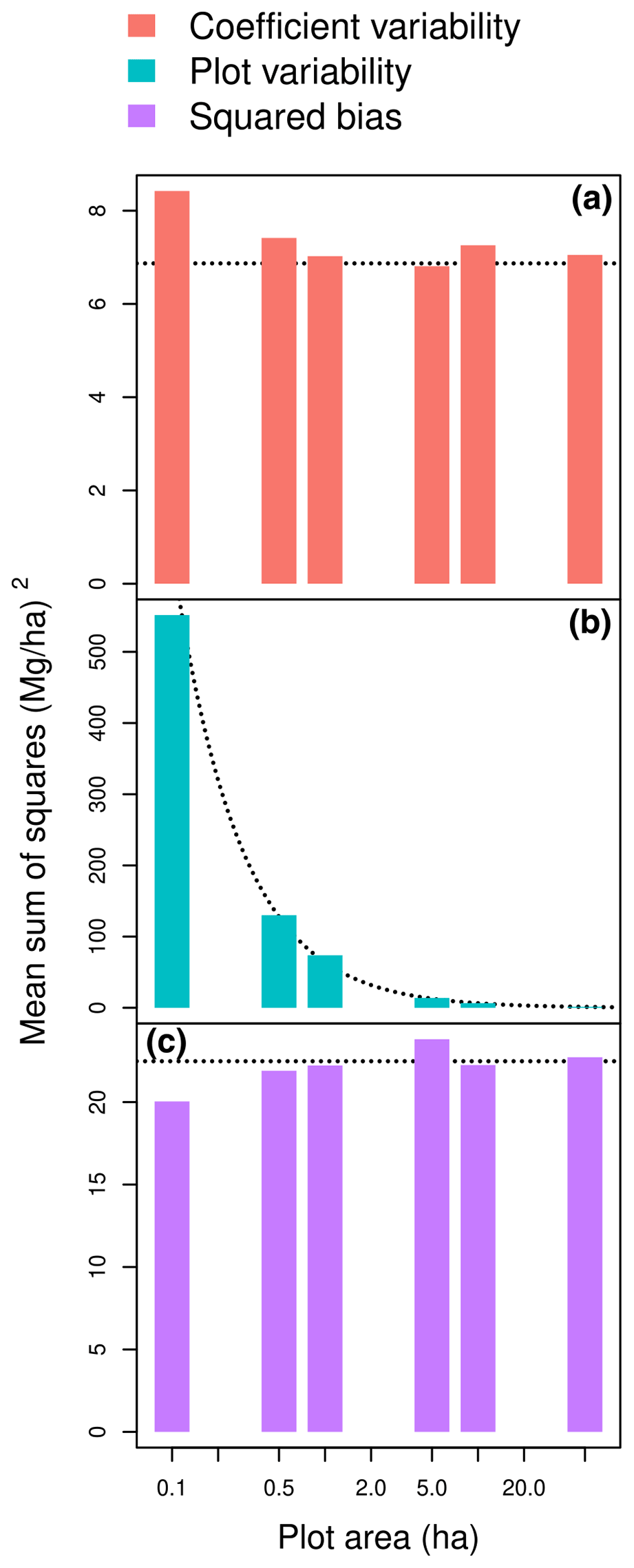
Figure 2 Coefficient variability (a), plot variability (b), and squared bias (c) as a function of plot area when predicting the aboveground biomass of a forest plot using the allometric equation $\ln \left(B\right)=a_{\mathrm{1}}+b_{\mathrm{1}}\ln \left(\mathit{\rho }{D}^{\mathrm{2}}H\right)$ fitted to a dataset of 844 trees in the Congo Basin. The dashed lines are (a) the horizontal line y=N² ME_ℱ; (b) the line $y=(N/A){\text{MSE}}_{\mathcal{F}}$, where A is the plot area; and (c) the horizontal line y=(Nb_ℱ)², where forest plots are randomly generated according to a null forest model ℱ with tree density N. The x axis has a log scale.

The plot-level predictive performance of a model thus depended on plot area. For a small plot area of 0.1 ha, MSS was dominated by its plot variability component (blue bars in Fig. 3a). Accordingly, the model with the lowest MSS was model (4), i.e., the model with the lowest $(N/A){\text{MSE}}_{\mathcal{F}}$. This selection agreed with the model selection based on tree-level performance statistics (Fig. 3a). The ranking of the five competing models based on their AIC (model (4) > (6) > (7) > (3) > (5)) was actually almost the same as their ranking based on their MSS for a plot size of 0.1 ha (model (4) > (6) > (3) > (7) > (5)). For a plot area of 1 ha, MSS was still dominated by its plot variability component, but the other components of MSS (violet and orange bars in Fig. 3b) gained in importance. Model (4), which had a large prediction bias, was outperformed by model (7), which had the smallest prediction bias among the five models. For a large plot area of 10 ha, the plot variability component of MSS was no longer decisive in model selection (Fig. 3c). Thanks to its small prediction bias and coefficient variability, model (7) again outperformed the other models.

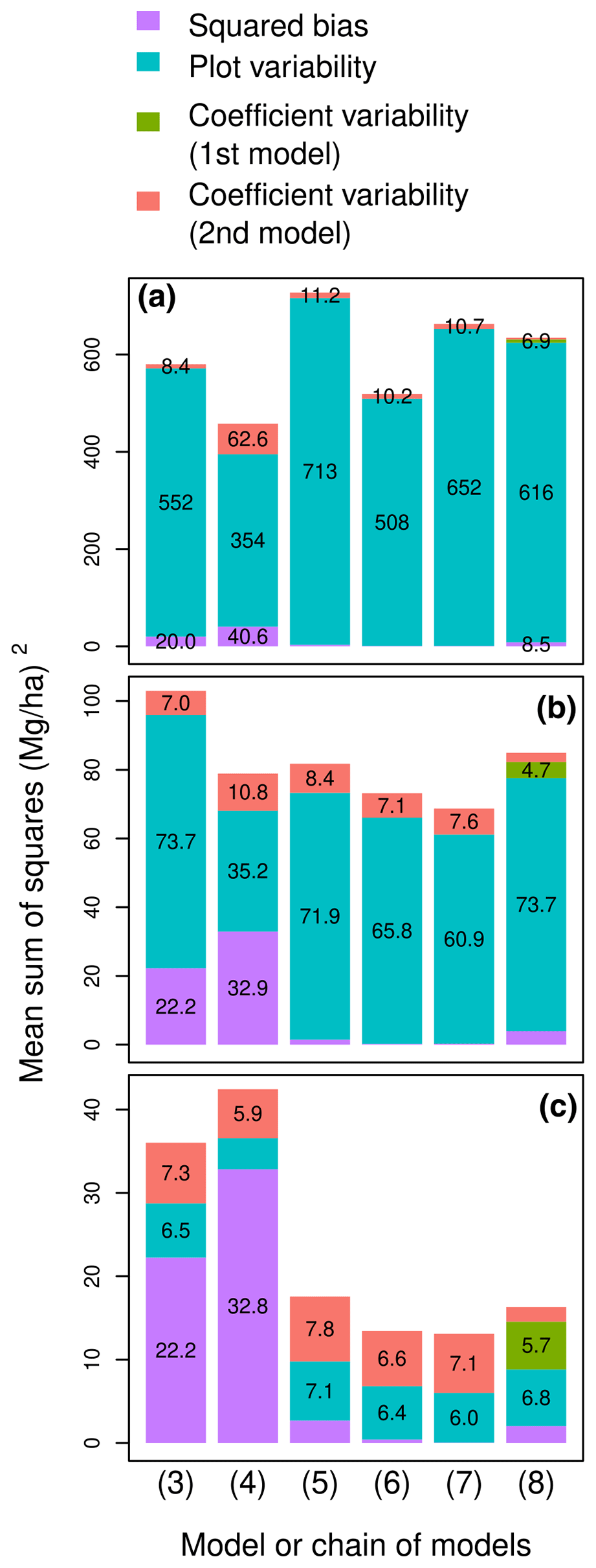
Figure 3 Partition of the mean sum of squared errors into squared bias, plot variability, the variability due to the coefficients of the first model, and the variability due to the coefficients of the second model for six models or model chains (labeled on the x axis) and for plots of area (a) A = 0.1 ha, (b) A = 1 ha, and (c) A = 10 ha. Errors are the differences between observed and predicted plot-level aboveground biomass. Model labels follow the model numbering in Table 2: (3) $\ln \left(B\right)=a_{\mathrm{1}}+b_{\mathrm{1}}\ln \left(\mathit{\rho }{D}^{\mathrm{2}}H\right)$; (4) $\ln \left(B\right)=a_{\mathrm{2}s}+b_{\mathrm{2}s}\ln \left(\mathit{\rho }{D}^{\mathrm{2}}H\right)$; (5) $\ln \left(B\right)=a_{\mathrm{3}}+b_{\mathrm{3}}\ln \left(\mathit{\rho }\right)+c_{\mathrm{3}}\ln \left(D\right)$; (6) $\ln \left(B\right)=a_{\mathrm{4}}+b_{\mathrm{4}}\ln \left(\mathit{\rho }\right)+c_{\mathrm{4}}\ln \left(D\right)+d_{\mathrm{4}}\ln \left(H\right)$; (7) $\ln \left(B\right)=a_{\mathrm{5}}+b_{\mathrm{5}}\ln \left(\mathit{\rho }\right)+c_{\mathrm{5}}\ln \left(D\right)+d_{\mathrm{5}}\ln \left(H\right)+e_{\mathrm{5}}\left[\ln \right(D){]}^{\mathrm{2}}$; (8) chain (f∘g), with g: $\ln \left(H\right)=a_{\mathrm{6}}+b_{\mathrm{6}}\ln \left(D\right)$ and f: $\ln \left(B\right)=a_{\mathrm{1}}+b_{\mathrm{1}}\ln \left(\mathit{\rho }{D}^{\mathrm{2}}H\right)$.

The choice of whether or not to add a variable to a model's predictors therefore depended on the level considered and the plot size. According to the F-test to compare nested models, which is a tree-level approach, model (6) outperformed model (5) (F=165.5 with 841 and 840 df, p value < 0.001). In other words, adding tree height on top of wood specific gravity and tree diameter in the model predictors improved the predictive performance of the model at the tree level. Whatever the plot area, the same conclusion was reached when comparing these two models at the plot level using MSS (compare models (5) and (6) in Fig. 3). However, model comparison based on MSS did not always agree with the F-test. All sorts of disagreement could be found. Tree-level prediction could be improved by adding the variable, while plot-level prediction was not. On the contrary, tree-level prediction was not improved by adding the variable, while plot-level prediction was. The variable “genus” illustrated the former disagreement: model (4) outperformed model (3) at the tree level (F=5.45 with 842 and 746 df, p value < 0.001). At the plot level, for a large plot area (10 ha), the performance ranking of the two models reversed (compare models (3) and (4) in Fig. 3c). The variable log (D)² illustrated the latter disagreement: model (7) did not outperform model (6) at the tree level (F=0.20 with 840 and 839 df, p value = 0.66). At the plot level, the opposite conclusion was obtained for plot areas of 1 and 10 ha (compare models (6) and (7) in Fig. 3).

Adding tree height as a predictor through a chain of models improved plot-level predictive performances for large plots. There is no F-test or goodness-of-fit statistic to compare a chain of models to a model. However, the MSS allowed us to compare the models to the two-step chain where tree height was first predicted from tree diameter, then biomass was predicted from wood specific gravity, diameter, and height. Predicting tree height from diameter using a larger dataset reduced the prediction bias but brought some additional variability due to the coefficients of the height–diameter model. The model based on diameter alone outperformed the chain for a plot area of 1 ha (compare (5) and (8) in Fig. 3). However, as plot area increased and plot variability vanished, the chain performed better than the model based on diameter alone.

4 Discussion

4.1 Predictive performance statistics

Forest-level predictive performance statistics were quite different from tree-level ones. Model selection for allometric equations has so far been based on tree-level predictive performance, such as AIC, residual standard error, and RMSE (e.g. Chave et al., 2014). Using forest-level performance statistics may thus shed new light on the selection of allometric equations among competing models. The different weighting of trees in the dataset and in the null forest changed the performance statistics. For instance, large trees had a much stronger weight in the dataset 𝒳 than in the null forest ℱ. Therefore, models that are biased for large trees will counter-perform according to b_𝒳 but show better performance according to b_ℱ. This result also implies that different forests will yield different performance statistics. In particular, the diameter distribution of trees in the forest will influence the forest-level performance statistics.

A significant result of our study was that the performance of a model to predict the biomass of a plot depended on plot size. This result is consistent with previous results based on error propagation (Chave et al., 2004). The plot-level performance statistics were good proxies of the MSS partition. Rather than performing long Monte Carlo computations to obtain MSS, one can immediately approximate it as $(N{b}_{\mathcal{F}}{)}^{\mathrm{2}}+(N/A){\text{MSE}}_{\mathcal{F}}+N^{\mathrm{2}}{\text{ME}}_{\mathcal{F}}$. This formula readily explains the change in MSS with plot size. For small plots, the predictive performance according to MSS is determined by the forest-level mean squared error MSE_ℱ. For large plots, individual tree errors compensate each other and cancel off, so MSE_ℱ no longer matters for the predictive performance. The predictive performance is then determined by the prediction bias and the variability due to model coefficients. In other words, models with high residual standard error are strongly penalized in tree-level selection, whereas it is much less a selection criterion in plot-level selection for large plots. When predicting the biomass of a large plot, what matters is the prediction bias and the coefficient variability.

When developing allometric equations, a recurring question is whether it is worth adding a variable among the set of predictors of a model (Feldpausch et al., 2012; Goodman et al., 2014). This question is equivalent to comparing two nested models, one with the variable among its predictors and the other without. When there was strong indication that adding the variable improved the prediction of the biomass of trees, the same conclusion was reached when considering the biomass of plots. However, when the benefit from adding the variable was not so marked, the conclusion based on tree-level prediction could differ from that based on plot-level prediction. Adding a predictor is all the more relevant, as it explains biomass variability. Alternatively, at the plot level, this variability can be left as a random noise that cancels off if the plot is large enough. It is thus a question of trade-off between bias and variance. The variable “genus” illustrates this trade-off here. Model (4), which fits a different allometry for each species genus, had the best tree-level predictive performance. It confirmed that different tree genera had different biomass allometries. However, at the scale of the forest where the species composition was not exactly the same as in the calibration dataset, model (4) resulted in the highest bias and the weakest overall predictive performance. In this example, we conclude that, even there are differences in allometry between tree genera, if our objective is to predict the biomass of large plots, it is statistically more efficient to leave the heterogeneity in species composition as a random noise.

Using plot-level predictive performance is desirable to predict plot biomass. However, to disentangle the biological processes that contribute to biomass allometry, goodness of fit should still be assessed at the tree level. The models we compared were all rooted in the allometry concept. Another family of models that predict tree-level biomass consists of geometric models, which are rooted in the tree taper concept. They predict biomass as wood density times volume, where volume is integrated from a taper equation (Manso et al., 2024). Another family of models emerges from the carbon allocation strategy of trees (Wolf et al., 2011; Yang et al., 2024). These different model families must be compared against the observations to build a theory of allometry.

One limitation of our study is that measurement errors were not taken into account in the MSS. However, measurement errors generally have a minor contribution to the overall biomass prediction error at the plot level (Chave et al., 2004). Another limitation is that simulated forests instead of real forest inventory data were used to generate plot data. We expect the bias contribution to MSS to increase with plot size for real data instead of being almost independent of it (Fig. 2c). If this hypothesis is verified, our results would be conservative with respect to the role of bias in model selection.

4.2 Validation datasets

We created this study in the context of model fitting, i.e., when a calibration dataset is available and model coefficients need to be estimated. A different context is when models are given with known coefficients and a validation dataset is available to compare their predictive performance. The MSS computations can take place in both contexts. Nonetheless, for a calibration dataset, by construction, model residuals sum up to zero. This property ensures that there is no prediction bias, at least for log-transformed variables and with equal tree weights in the dataset. This is no longer true with a validation dataset. If the trees used to fit the model are not representative of the area where the allometric equation is applied, it will lead to prediction bias. To exemplify this bias, we can fit the allometric equation using dataset 𝒳, whose trees come from central Africa, and assess its predictive performance using the subset of dataset 𝒳^′ corresponding to the Amazon (with trees coming from Brazil, Colombia, French Guiana, and Peru). The coefficient variability and the plot variability were of the same order for Amazonian forests as for central African forests (Fig. 4a). However, the bias component was about 30 times greater for Amazonian forests than for central African forests, thus confirming that central African forests differed from Amazonian forests. Therefore, assessing the predictive performance of the allometric equations on a dataset that is not representative of the forest where the equations were fitted inflates the role of bias in the overall performance.

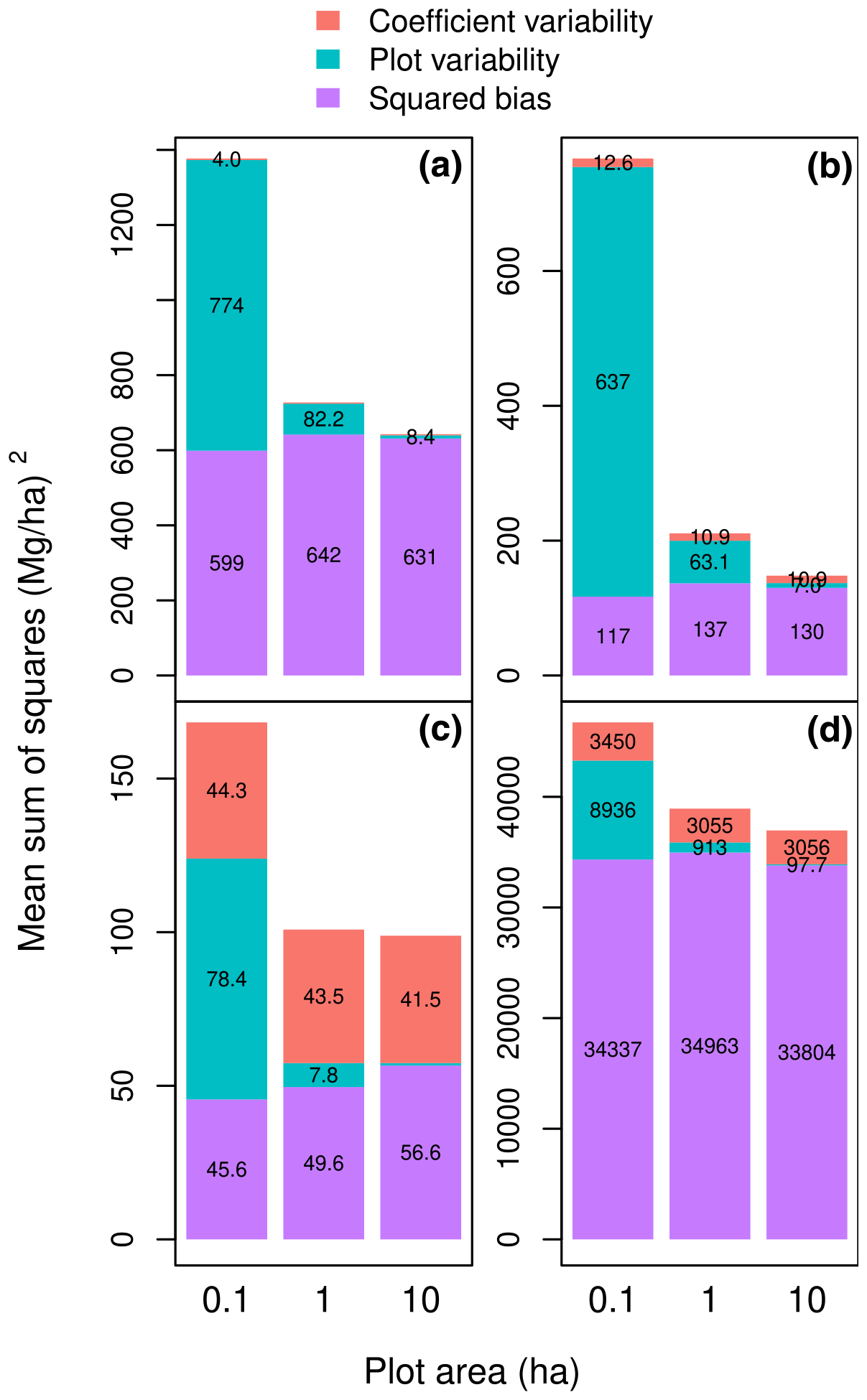
Figure 4 Partition of the mean sum of squared errors (MSS) into squared bias, plot variability, and the variability due to the model coefficients when the dataset used for model fitting differs from the dataset used to compute MSS: (a) the calibration dataset is the dataset 𝒳 of Fayolle et al. (2018), and the validation dataset is a subset of the dataset of Chave et al. (2014) corresponding to the Amazon; (b) the calibration dataset is 𝒳, and the validation dataset is the subset of 𝒳 with the slenderest trees (i.e., excluding trees less than 0.9 × the average tree height); (c) the calibration dataset is the subset of 𝒳 with the largest trees (D≥ 48.9 cm), and the validation dataset is the subset of 𝒳 with the smallest trees (D < 48.9 cm); (d) the calibration dataset is the subset of 𝒳 with the smallest trees (D < 48.9 cm), and the validation dataset is the subset of 𝒳 with the largest trees (D≥ 48.9 cm). The model is $\ln \left(B\right)=a_{\mathrm{1}}+b_{\mathrm{1}}\ln \left(\mathit{\rho }{D}^{\mathrm{2}}H\right)$, and the plot area varies from 0.1 to 10 ha (on the x axis). Errors are the differences between observed and predicted plot-level aboveground biomass.

If some model predictors vary in a systematic way (i.e., non-randomly) across plots in the validation dataset, then the model residuals will also result in a plot-level prediction bias. To illustrate this effect, consider a pseudo-validation dataset 𝒱 that is resampled from 𝒳 using weights w_i given by Eq. (1) but with the additional condition that a tree is sampled if its height is greater than the 9/10 of the average height predicted by model (2). Dataset 𝒱 is not a true validation dataset because it is built from the calibration dataset 𝒳. Nonetheless, it illustrates what would happen if a validation dataset was taken from a plot where trees were systematically more slender than in the calibration plots. Then, the squared bias component of the MSS is indeed inflated. For model (3), it increases from 22 to 130 Mg² ha⁻² (Fig. 4b; to be compared to model (3) in Fig. 3).

A similar approach can be used to assess the prediction error when predictors extend beyond the calibration range. To illustrate this effect, we partitioned dataset 𝒳 into a subset of large trees with diameter ≥ 48.9 cm and a subset of small trees with diameter < 48.9 cm, where 48.9 cm is the median diameter of trees in 𝒳. One subset was then used for model fitting, and the other one was used to compute MSS. The error of predicting the biomass of large trees with an allometric equation fitted to small trees was much greater than the error of predicting the biomass of small trees with an allometric equation fitted to large trees (Fig. 4c and d). Moreover, the bias was comparatively greater in the former case than in the latter case. Due to heteroscedasticity, there is much more variability in tree biomass in large trees than in small trees. Including large trees in biomass datasets is a recommendation that has long been known (Chave et al., 2005).

4.3 Local specific versus general equations

Our results can contribute to the long-standing debate about locally developed specific equations versus general allometric equations (Chave et al., 2004; Weiskittel et al., 2015). Given a maximum sampling effort, and thus a given amount of available observations, the question is whether observations should be split among different categories (typically species and sites) to fit locally developed specific equations or whether observations should be kept together to fit a general equation. Locally developed specific equations tend to be less biased (Weiskittel et al., 2015). However, because they are based on a smaller number of observations, they tend to have a greater residual error and a greater variability due to coefficients. Our results indicate that the answer to this question also depends on the size of the plots for which biomass is predicted. Larger plots penalize biased models more heavily. They thus tend to favor locally developed specific equations. Our results also show that, in up to 1 ha of plot area, the plot variability is the dominant component of MSS. Because this component of MSS is the one related to the residual model error, it indicates that general allometric equations would tend to be preferred to predict the biomass of plots with an area less than or equal to 1 ha. This conclusion would have to be confirmed using other datasets.

A variant of this question is whether or not to add an extra variable (typically tree height) as a predictor of the model (Feldpausch et al., 2012). The extra variable can better account for local variation in biomass, thus reducing bias. On the other hand, the requirement for this variable may reduce the availability of data, thus increasing residual error and the variability due to coefficients. Using a chain of models where the extra variable is first predicted from other predictors (typically tree height predicted from diameter) can circumvent this problem (Chave et al., 2014; Sullivan et al., 2018). Typically, the first model (the height–diameter relationship) is locally fitted, while the second model (the biomass equation) is a general equation, thus combining the advantages of locally fitted models with those of general models. We showed here that this strategy could indeed be efficient, even for a single calibration dataset.

5 Conclusions

The plot-level predictive performance of an allometric equation depended on plot size. The effect of plot size A could be well approximated by the formula $(N{b}_{\mathcal{F}}{)}^{\mathrm{2}}+(N/A){\text{MSE}}_{\mathcal{F}}+N^{\mathrm{2}}{\text{ME}}_{\mathcal{F}}$, where the first term corresponds to bias, the second corresponds to the tree residual error, and the third one corresponds to the uncertainty on model coefficients. For small plots (≤ 0.1 ha), the plot-level predictive performance was dominated by the MSE_ℱ term. Model selection based on plot-level predictive performance was then consistent with model selection based on tree-level performance. For large plots, the term depending on MSE_ℱ vanished. Model selection based on plot-level performance could then differ from that based on tree-level performance. In the case of large plots, chains of models that combined a general equation to predict biomass and local equations to predict some of the predictors of the biomass equation could provide a good trade-off between the bias and the uncertainty in model coefficients. For these large plots, introducing additional covariates in the models may not be needed. The unexplained share of biomass variability may instead be left as a random noise that cancels off among trees. Our results may thus contribute to save efforts in measuring tree biomass for the future development of allometric equations.

Appendix A: Decomposition of the mean sum of squares

A1 One-model decomposition

For one model, the mean sum of squares of differences between observed and predicted plot-level biomass is

$$\begin{array}{}\text{(A1)}& \text{MSS}={\displaystyle \frac{\mathrm{1}}{KJ}}\sum _{k=\mathrm{1}}^K\sum _{j=\mathrm{1}}^J{e}_{kj}^{\mathrm{2}}.\end{array}$$

By the definition of the variance, the mean sum of squares is equal to the variance plus the squared bias. As the plot area tends to infinity, the number of trees goes to infinity and the difference between the plot-level observed biomass and the predicted one tends towards the forest-level bias times the number of trees in the plot. Thus MSS = Var + SB, where

$$\begin{array}{}\text{(A2)}& {\displaystyle }\text{SB}& {\displaystyle }={\stackrel{\mathrm{‾}}{e}}^{\mathrm{2}}=({\displaystyle \frac{\mathrm{1}}{KJ}}\sum _{k=\mathrm{1}}^K\sum _{j=\mathrm{1}}^J{e}_{kj}{)}^{\mathrm{2}}\approx (N{b}_{\mathcal{F}}{)}^{\mathrm{2}},\text{(A3)}& {\displaystyle }\text{Var}& {\displaystyle }={\displaystyle \frac{\mathrm{1}}{KJ}}\sum _{k=\mathrm{1}}^K\sum _{j=\mathrm{1}}^J(e_{kj}-\stackrel{\mathrm{‾}}{e}{)}^{\mathrm{2}}.\end{array}$$

Using the calculations of the analysis of variance, the variance can in turn be partitioned into an inter-plot variance (or plot variability) and an intra-plot variance. The variability in plot-level biomass errors results from the individual tree errors that do not compensate. Therefore, the greater the residual standard error of model f, the greater this plot variability. As the plot area tends to infinity, the tree-level errors from different trees compensate each other and the plot variability vanishes. As the plot area tends to zero, the tree-level errors from different trees do not compensate. For a very small plot area, the plot contains very few trees whose errors accumulate almost independently. Therefore, the plot-level variance of biomass differences is close to the sum of individual errors: NA×MSE_ℱ. Scaling this error per unit area of the plot finally brings $(N/A){\text{MSE}}_{\mathcal{F}}$.

Regarding the intra-plot variance (or variability within a plot), it results from the different coefficient values and reflects the uncertainty on these coefficients. For a tree taken at random in the forest with probability w_i, the difference in biomass due to a model coefficient θ_j is ${\sum }_{i=\mathrm{1}}^m{w}_i\left[f\right({\mathit{x}}_i,\mathit{\theta })-f({\mathit{x}}_i,{\mathit{\theta }}_j\left)\right]$. For the NA trees found in a plot with area A, this difference is multiplied by NA. Integrating over the possible outcomes of θ_j and scaling per unit area of the plot, it shows that the coefficient variability is close to N² ME_ℱ.

To summarize, Var = (plot variability) + (coefficient variability), where

$$\begin{array}{}\text{(A4)}& {\displaystyle }\begin{array}{rl}\text{plot variability}& ={\displaystyle \frac{\mathrm{1}}{K}}\sum _{k=\mathrm{1}}^K({\stackrel{\mathrm{‾}}{e}}_{k.}-\stackrel{\mathrm{‾}}{e}{)}^{\mathrm{2}}\\ & \approx (N/A){\text{MSE}}_{\mathcal{F}},\end{array}\text{(A5)}& {\displaystyle }\begin{array}{rl}\text{coefficient variability}& ={\displaystyle \frac{\mathrm{1}}{KJ}}\sum _{k=\mathrm{1}}^K\sum _{j=\mathrm{1}}^J(e_{kj}-{\stackrel{\mathrm{‾}}{e}}_{k.}{)}^{\mathrm{2}}\\ & \approx N^{\mathrm{2}}{\text{ME}}_{\mathcal{F}},\end{array}\text{(A6)}& {\displaystyle }{\stackrel{\mathrm{‾}}{e}}_{k.}={\displaystyle \frac{\mathrm{1}}{J}}\sum _{j=\mathrm{1}}^J{e}_{kj}.\end{array}$$

A2 Two-model decomposition

For a chain of two models, the mean sum of squares of differences between observed and predicted plot-level biomass is

$$\begin{array}{}\text{(A7)}& \text{MSS}={\displaystyle \frac{\mathrm{1}}{KLJ}}\sum _{k=\mathrm{1}}^K\sum _{l=\mathrm{1}}^L\sum _{j=\mathrm{1}}^J{e}_{klj}^{\mathrm{2}}.\end{array}$$

As before, the mean sum of squares is the variance plus the squared bias, MSS = Var + SB, where

$$\begin{array}{}\text{(A8)}& {\displaystyle }\text{SB}& {\displaystyle }={\stackrel{\mathrm{‾}}{e}}^{\mathrm{2}}=({\displaystyle \frac{\mathrm{1}}{KLJ}}\sum _{k=\mathrm{1}}^K\sum _{l=\mathrm{1}}^L\sum _{j=\mathrm{1}}^J{e}_{klj}{)}^{\mathrm{2}},\text{(A9)}& {\displaystyle }\text{Var}& {\displaystyle }={\displaystyle \frac{\mathrm{1}}{KLJ}}\sum _{k=\mathrm{1}}^K\sum _{l=\mathrm{1}}^L\sum _{j=\mathrm{1}}^J(e_{klj}-\stackrel{\mathrm{‾}}{e}{)}^{\mathrm{2}}.\end{array}$$

Again, the variance can be partitioned into an inter-plot variance (or plot variability) and an intra-plot variance (or coefficient variability), Var = (plot variability) + (coefficient variability), where

$$\begin{array}{}\text{(A10)}& {\displaystyle }\text{plot variability}={\displaystyle \frac{\mathrm{1}}{K}}\sum _{k=\mathrm{1}}^K({\stackrel{\mathrm{‾}}{e}}_{k..}-\stackrel{\mathrm{‾}}{e}{)}^{\mathrm{2}},\text{(A11)}& {\displaystyle }\begin{array}{rl}\text{coefficient variability}=& {\displaystyle \frac{\mathrm{1}}{KLJ}}\sum _{k=\mathrm{1}}^K\sum _{l=\mathrm{1}}^L\sum _{j=\mathrm{1}}^J\\ & \times (e_{klj}-{\stackrel{\mathrm{‾}}{e}}_{k..}{)}^{\mathrm{2}},\end{array}\text{(A12)}& {\displaystyle }{\stackrel{\mathrm{‾}}{e}}_{k..}={\displaystyle \frac{\mathrm{1}}{LJ}}\sum _{l=\mathrm{1}}^L\sum _{j=\mathrm{1}}^J{e}_{klj}.\end{array}$$

Now the coefficient variability can be partitioned into the variability due to the coefficients of model g and that due to the coefficients of model f, (coefficient variability) = (variability due to g coefficients) + (variability due to f coefficients), where

$$\begin{array}{}\text{(A13)}& {\displaystyle }\begin{array}{rl}\text{variability due to }& g\text{ coefficients}\\ & ={\displaystyle \frac{\mathrm{1}}{KL}}\sum _{k=\mathrm{1}}^K\sum _{l=\mathrm{1}}^L({\stackrel{\mathrm{‾}}{e}}_{kl.}-{\stackrel{\mathrm{‾}}{e}}_{k..}{)}^{\mathrm{2}},\end{array}\text{(A14)}& {\displaystyle }\begin{array}{rl}\text{variability due to }& f\text{ coefficients}\\ & ={\displaystyle \frac{\mathrm{1}}{KLJ}}\sum _{k=\mathrm{1}}^K\sum _{l=\mathrm{1}}^L\sum _{j=\mathrm{1}}^J(e_{klj}-{\stackrel{\mathrm{‾}}{e}}_{kl.}{)}^{\mathrm{2}},\end{array}\text{(A15)}& {\displaystyle }{\stackrel{\mathrm{‾}}{e}}_{kl.}={\displaystyle \frac{\mathrm{1}}{J}}\sum _{j=\mathrm{1}}^J{e}_{klj}.\end{array}$$