A microbially driven and depth-explicit soil organic carbon model constrained by carbon isotopes to reduce parameter equifinality

Over the past years, microbially driven models have been developed to improve simulations of soil organic carbon (SOC) and have been put forward as an improvement to assess the fate of SOC stocks under environmental change. While these models include a better mechanistic representation of SOC cycling compared to cascading-reservoir-based approaches, the complexity of these models implies that data on SOC stocks are insufficient to constrain the additional model parameters. In this study, we constructed a novel depth-explicit SOC model (SOILcarb – Simulation of Organic carbon and its Isotopes by Linking carbon dynamics in the rhizosphere and bulk soil) that incorporates multiple processes influencing the δ¹³C and Δ¹⁴C values of SOC. This was used to assess if including data on the δ¹³C and Δ¹⁴C values of SOC during parameter optimisation reduces model equifinality, the phenomenon that multiple parameter combinations lead to a similar model output. To do so, we used SOILcarb to simulate depth profiles of total SOC and its δ¹³C and Δ¹⁴C values. The results show that when the model is calibrated based on only SOC stock data, the residence time of subsoil organic carbon (OC) is not simulated correctly, thus effectively making the model of limited use to predict SOC stocks driven by, for example, environmental changes. Including data on δ¹³C in the calibration process reduced model equifinality only marginally. In contrast, including data on Δ¹⁴C in the calibration process resulted in simulations of the residence time of subsoil OC being consistent with measurements while reducing equifinality only for model parameters related to the residence time of OC associated with soil minerals. Multiple model parameters could not be constrained even when data on both δ¹³C and Δ¹⁴C were included. Our results show that equifinality is an important phenomenon to consider when developing novel SOC models or when applying established ones. Reducing uncertainty caused by this phenomenon is necessary to increase confidence in predictions of the soil carbon–climate feedback in a world subject to environmental change.

1 Introduction

Soils are an important component of the global carbon cycle, storing a vast amount of organic carbon (OC) (Scharlemann et al., 2014; Ciais et al., 2013). However, it is often overlooked that about 77 % of the soil organic carbon (SOC) in the upper 3 m of soil is present below a depth of 0.3 m (Lal, 2018). Furthermore, while topsoil (< 0.3 m depth) OC is generally characterised by average residence times ranging from years to decades (Baisden et al., 2013; Schrumpf and Kaiser, 2015), subsoil (> 0.3 m depth) OC typically has residence times of up to centuries or millennia (Balesdent et al., 2018; Luo et al., 2019). Despite these long residence times, subsoil OC is likely to play an important role in the climate–soil carbon feedback, as subsoil OC has been shown to be susceptible to losses upon soil warming (Hicks Pries et al., 2017; Soong et al., 2021; Jia et al., 2019). A correct representation of the rate of OC cycling along the soil profile in biogeochemical models is necessary to make accurate predictions about climate–soil carbon feedbacks. When these rates are overestimated, the simulated size of the SOC stock will adapt too fast to changes in OC inputs. This leads to an underestimation of the time it takes for soils to increase their OC storage due to increases in, for example, net primary productivity or OC inputs in agroecosystems (He et al., 2016; Wang et al., 2019).

Classical models simulating subsoil OC dynamics are based on conceptual pools with intrinsic turnover times, with the simulated carbon generally cascading along a sequence of model pools. The rate of OC turnover is generally calculated as a function of abiotic factors and the chemistry of organic compounds. Such models have been developed as stand-alone models (e.g. Elzein and Balesdent, 1995; Ota et al., 2013; Wang et al., 2015) or have been incorporated in ecosystem models (e.g. Camino-Serrano et al., 2018; Koven et al., 2013). These biogeochemical models have been criticised, as they do not incorporate the emerging understanding of the controls on soil organic carbon (SOC) dynamics (Blankinship et al., 2018; Schmidt et al., 2011; Dungait et al., 2012; Bradford et al., 2016). For example, these models do not explicitly simulate soil microbes, which are both decomposers and important precursors of stabilised SOC (Denef et al., 2010; Kästner and Miltner, 2018; Kögel-Knabner, 2002; Six et al., 2006), and organo-mineral associations, which protect SOC from decomposition (Kleber et al., 2015, 2021; Sollins et al., 1996). In addition, model pools with a strong inherent recalcitrance, such as the “passive pool” in models such as DayCent (Parton et al., 1987) and the “humified organic matter pool” in RothC (Coleman et al., 1997), are assumed to be the result of humification, a theory that is being considered flawed and obsolete (Kleber and Lehmann, 2019; Lehmann and Kleber, 2015).

As a reaction to this emerging understanding of the controls on SOC dynamics over the past decades, several mechanistic, microbially driven models simulating depth profiles of SOC have been developed (e.g. Ahrens et al., 2015, 2020; Dwivedi et al., 2017; Riley et al., 2014; Yu et al., 2020; Zhang et al., 2021). These models share multiple characteristics, such as the explicit representation of soil microbes and the protection of SOC by association with soil minerals. Moreover, the increasing residence time of SOC with soil depth is simulated as an emerging function of biotic and abiotic soil properties (Ahrens et al., 2020). This improves the mechanistic representation of SOC dynamics in these models compared to first-order decay models, which generally use an exponentially decreasing parameter with depth to force the decreasing processing rate of SOC along the soil profile (Koven et al., 2013; Wang et al., 2015, 2020).

This new generation of SOC models is characterised by an increase in model complexity and in the number of model parameters (Campbell and Paustian, 2015; Lawrence et al., 2009). This is an important consideration, as an increase in parameter uncertainty can outweigh model improvements due to a better mechanistic description of the system, thereby increasing the overall model error (Van Rompaey and Govers, 2002). Finding an optimal balance between errors related to process representation and data availability is of major importance to create confidence in model outputs (Schindler and Hilborn, 2015). A model that is too complex with respect to the availability of data can result in multiple combinations of parameter values that lead to a near-optimal solution, so-called “behavioural models”. This phenomenon has been referred to in the literature by multiple terms, such as equifinality (e.g. Beven, 2006, 1993), non-uniqueness (Beven, 2006) or non-identifiability of model parameters (Brun et al., 2001; Sierra et al., 2015). Equifinality is a major issue for models simulating hydrology (e.g. Beven and Freer, 2001), SOC (e.g. Sierra et al., 2015; Braakhekke et al., 2013; Marschmann et al., 2019), soil nitrogen (e.g. Schulz et al., 1999) and ecosystem models in general (e.g. Luo et al., 2009; Tang and Zhuang, 2008). In the case of SOC models, models characterised by equifinality are often able to make correct predictions of steady-state SOC stocks, although these stocks can be predicted by different distributions of SOC among the simulated model pools (Braakhekke et al., 2013). The problems (and uncertainty) arise when different behavioural models are used to make predictions of SOC stocks based on changing environmental conditions or OC inputs. In this case, behavioural models starting from an identical initial SOC stock can produce a wide range of predicted values, from which it is generally not possible to identify the correct model (and parameter set) (Luo et al., 2016, 2017). In the present article, we use the term parameter equifinality for this phenomenon. In addition, the term overparameterisation is used for the situation when the number of model parameters is too large with respect to the available observational support for the processes represented by these parameters.

One way to reduce parameter equifinality is to include additional constraints on model parameter values during the calibration process (Braakhekke et al., 2014). This has been done for multiple classical SOC models by simulating, in addition to total SOC, depth profiles of the ratio of stable carbon isotopes (δ¹³C) (Amundson and Baisden, 2000; van Dam et al., 1997; Poage and Feng, 2004), radioisotopes (Δ¹⁴C) (Baisden and Parfitt, 2007; Jenkinson and Coleman, 2008; Koven et al., 2013; Tifafi et al., 2018; Braakhekke et al., 2014), a combination of both (Wang et al., 2020; Baisden et al., 2002) or ²¹⁰Pb (Braakhekke et al., 2013). Some mechanistic models also simulate the behaviour of ¹⁴C (Ahrens et al., 2015, 2020; Dwivedi et al., 2017; Yu et al., 2020). While it has been shown that simulating these additional variables puts meaningful constraints on parameter values, measurements of the necessary data are costly and hence such data are not widely available. On the other hand, δ¹³C isotope ratios can be rapidly and relatively cheaply measured. While these isotopes do not decay radioactively like ¹⁴C, multiple processes that take place over decadal to centennial timescales influence depth patterns of the δ¹³C value of SOC. For example, it has been shown that long-term changes in the δ¹³C value of vegetation (Keeling, 1979; Schubert and Jahren, 2015) influence the δ¹³C value of SOC along the depth profile considerably (Paul et al., 2019). In addition, there is evidence that microbial necromass, which constitutes up to 50 % SOC (Rumpel and Kögel-Knabner, 2010; Wang et al., 2021; Angst et al., 2021), is generally enriched in ¹³C compared to their substrate (Dijkstra et al., 2006; Gleixner et al., 1993; Miltner et al., 2004). Explicitly simulating the fate of microbial necromass and its ¹³C isotopes therefore has the potential to better constrain the rate of the formation of stabilised microbial necromass in soils (Šantrůčková et al., 2018). Lastly, as above- and belowground C inputs to the soil generally have different δ¹³C values (Bowling et al., 2008; Werth and Kuzyakov, 2010), simulating the δ¹³C value of these inputs has the potential to better constrain the vertical mixing of OC from different sources along the soil profile. To the best of our knowledge, the potential of using ¹³C isotope data to constrain the parameter values of a microbially driven and depth-explicit SOC model has to date not been explored.

Therefore, the aim of this study is to assess to what extent the simulation of the δ¹³C and Δ¹⁴C values of SOC, in addition to SOC itself, allows model parameter values of a microbially driven and depth-explicit SOC model to be better constrained, thereby reducing model equifinality. To do so, we constructed a novel depth-explicit SOC model that incorporates multiple processes that influence the δ¹³C and Δ¹⁴C values of SOC. We hypothesised that (1) calibrating a microbially explicit model using only OC stock data results in substantial parameter equifinality and (2) underestimates the residence time of subsoil OC (following He et al., 2016), while (3) using simulated depth profiles of δ¹³C or Δ¹⁴C or a combination of both as additional constraints on parameter values will narrow the range of optimised parameter values, which results in behavioural models (i.e. a model solution that cannot easily be rejected). As the δ¹³C value of SOC is generally not simulated in mechanistic SOC models, we also discuss the effect of different mechanisms on simulated depth profiles of δ¹³C. As equifinality in SOC models has received only limited research attention, increasing awareness of, and solving, this problem will increase confidence in simulations of the role soils can play in climate change mitigation or increasing SOC stocks to improve soil health.

2 Materials and methods

2.1 The SOILcarb model

This section provides a brief description of the main processes simulated in SOILcarb (Simulation of Organic carbon and its Isotopes by Linking carbon dynamics in the rhizosphere and bulk soil). A detailed model description and overview of the equations are provided in the Supplement, as well as an overview of the state variables (Table S5 in the Supplement) and model parameters (Table S6). The R codes of SOILcarb are available from Van de Broek (2025). The presented version of SOILcarb was used to simulate depth profiles of OC dynamics in natural forest soils. We note that the main aim of the developed model for the present paper was to show the effect of equifinality on model outcomes and that the application of SOILcarb to other environments requires further testing.

The vertical soil profile is simulated down to 1 m depth for layers with an increasing thickness with depth. SOILcarb has been programmed in R (R Core Team, 2024), with the differential equations regulating the flows of OC being solved using the lsodes solver from the deSolve package (Soetaert et al., 2010). For the presented simulations, the model was run for a period of 15 000 years up to the year 2004. It is noted that the current model does not include the effect of temperature and soil moisture, limiting the model to predict SOC and its isotopic signature under steady-state environmental conditions.

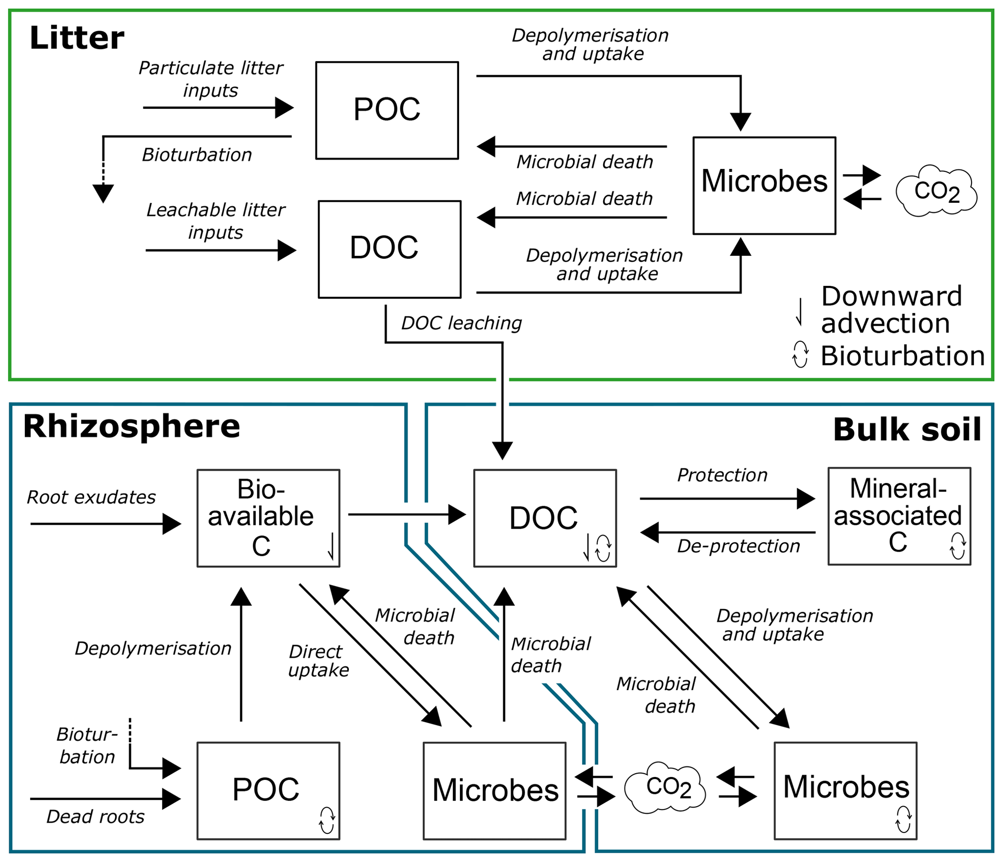
Figure 1 Conceptual model of SOILcarb showing the model pools and fluxes of organic carbon in the litter layer, rhizosphere and bulk soil. POC is particulate organic carbon; DOC is dissolvable organic carbon.

2.1.1 Simulation of organic carbon dynamics

SOILcarb is divided into three compartments: (1) litter layer, (2) rhizosphere and (3) bulk soil (Fig. 1). The litter layer is simulated spatially separated from the soil compartments. The rhizosphere and bulk soil compartments are used to conceptually separate the parts of the soil where most OC inputs occur and OC cycles relatively fast (the rhizosphere) from the zone where available OC for microbes is relatively limited due to mineral protection and where OC cycles relatively slow (the bulk soil). Inputs of OC in the litter layer originate from litterfall, which is separated into particulate OC (C_POC-l) and dissolvable OC (C_DOC-l). Depolymerisation and microbial uptake of C_POC-l and C_DOC-l are simulated using the equilibrium chemistry approximation (Tang and Riley, 2013) (the model assumes that dissolved organic carbon (DOC) needs to be depolymerised before uptake, as a considerable portion of DOC is generally not bio-available; Risse-Buhl et al., 2013; Shen et al., 2015; Andreasson et al., 2009), while microbial turnover is simulated as a logistic growth process (Georgiou et al., 2017). Microbial OC uptake in all compartments is reduced based on a fixed carbon use efficiency (CUE), with the remaining OC being transformed to CO₂. Carbon from the litter layer is transferred to the bulk soil through bioturbation of C_POC-l and leaching of C_DOC-l.

In the rhizosphere, OC inputs are separated into (1) rhizodeposits, providing bio-available OC (C_bioav-r) to the soil, and (2) root turnover, providing particulate OC (C_POC-r) to the soil. Depolymerisation of C_POC-r to C_bioav-r is simulated using reverse Michaelis–Menten kinetics, whereby the rate of depolymerisation is modified based on the ratio of microbes in the rhizosphere (C_mic-r) to C_POC-r (see Supplement). Uptake of C_bioav-r by C_mic-r is simulated using forward Michaelis–Menten kinetics, whereby the rate of OC uptake is modified based on the ratio of C_mic-r to C_bioav-r. Following microbial turnover in the rhizosphere (simulated using a logistic growth function), the soluble portion of microbial cells (the cytoplasm) is transferred back to C_bioav-r, while the non-soluble portion of microbial cells is transferred to the DOC pool in the bulk soil (C_DOC-b). A fixed portion of C_bioav-r is transferred to C_DOC-b to allow the direct adsorption of root-derived OC on soil minerals without first passing through a soil microbe. From C_DOC-b, OC can either be protected by adsorption on soil minerals (C_min-b), rendering it inaccessible to microbial uptake, or be taken up by microbes in the bulk soil (C_mic-b). Competition for C_DOC-b between minerals and microbes is simulated using the equilibrium chemistry approximation (Tang and Riley, 2013). De-protection of C_min-b is simulated as a first-order process. Vertical transport of OC along the soil profile occurs as (1) bioturbation, simulated as a diffusion process (for C_POC-r, C_DOC-b, C_min-b and C_mic-b), and (2) leaching, simulated as an advection process (for C_bioav-r and C_DOC-b). It has been shown that the rate of de-protection of mineral-associated OC is influenced by root exudates (Keiluweit et al., 2015). Therefore, the simulated rate of de-protection of OC from minerals is a function of the portion of the soil occupied by the rhizosphere, calculated following Finzi et al. (2015). In addition, the amount of mineral surfaces available for the protection of OC is scaled according to the rhizosphere volume (i.e. the larger the rhizosphere volume, the larger the surface of minerals which is in contact with OC originating from the rhizosphere).

2.1.2 Simulation of δ¹³C and Δ¹⁴C of organic carbon

In SOILcarb, fluxes of ¹³C and ¹⁴C between model pools follow fluxes of ¹²C. The model first calculates fluxes of ¹²C between pools and subsequently uses the ratio of ¹²C leaving every pool to the total amount of ¹²C of the respective pools to calculate how much ¹³C and ¹⁴C leave every pool:

$$\begin{array}{}\text{(1)}& F_{{}^{X}C}={}^X{C}_{\text{pool}}\cdot {\displaystyle \frac{F_{{}^{\mathrm{12}}\mathrm{C}}}{{}^{\mathrm{12}}{\mathrm{C}}_{\mathrm{pool}}}},\end{array}$$

where $F_{{}^{X}C}$ is the flux of ¹³C or ¹⁴C leaving a pool, $F_{{}^{\mathrm{12}}\mathrm{C}}$ is the previously calculated flux of ¹²C leaving the same pool, ^XC_pool is the amount of ¹³C or ¹⁴C in the pool which loses OC, and ¹²C_pool is the amount of ¹²C in the pool which loses OC. The model parameters are thus defined based on the ¹²C content of every pool.

The simulated processes that affect temporal variations in the δ¹³C value of SOC are (1) annual changes in the δ¹³C value of atmospheric CO₂, directly affecting the δ¹³C value of vegetation; (2) the effect of atmospheric CO₂ concentration on kinetic fractionation against ¹³C during plant photosynthesis; (3) differences in the δ¹³C value of aboveground plant biomass, belowground biomass and rhizodeposits; and (4) heterotrophic CO₂ assimilation by soil microbes. The same processes affect the temporal variation in the Δ¹⁴C of SOC, in addition to radioactive decay. Note that no preferential microbial mineralisation of ¹²C relative to ¹³C is simulated, as consistent empirical evidence for this is lacking (Boström et al., 2007; Ehleringer et al., 2000).

The difference in the δ¹³C value between atmospheric CO₂ and aboveground biomass is calculated for every time step as the sum of a fixed and variable component:

$$\begin{array}{}\text{(2)}& {\mathrm{diff}}^{\mathrm{13}}{\mathrm{C}}_{\mathrm{atm}\text{-}\mathrm{leaf}}\left(t\right)={\mathrm{diff}}_{\mathrm{fixed}}+{\mathrm{diff}}_{\mathrm{variable}}\left(t\right),\end{array}$$

where diff_fixed is a constant representing a fixed and user-provided difference in δ¹³C between atmospheric CO₂ and aboveground biomass, and diff_variable(t) represents the effect of atmospheric CO₂ concentration on kinetic fractionation against ¹³C during photosynthesis for every time step (see Sect. S1.6.3 in the Supplement).

The value of diff_fixed is provided by the user for the last simulation year and is assumed to be constant throughout the simulation. For every simulated time step, the δ¹³C value of aboveground biomass is subsequently calculated from a long-term series of average annual δ¹³C values of atmospheric CO₂, which was compiled from Schmitt et al. (2012), Bauska et al. (2015), and Graven et al. (2017) (see Fig. S2 in the Supplement). The annual Δ¹⁴C value of OC inputs from aboveground biomass is determined from a compiled series of annual average Δ¹⁴C values of atmospheric CO₂ (from Reimer et al., 2013; Hua et al., 2013; Hammer and Levin, 2017; see Fig. S3). It was assumed that during photosynthesis, the fractionation against ¹⁴CO₂ is twice that of ¹³CO₂, as the mass difference between ¹⁴CO₂ and ¹²CO₂ is twice that between ¹³CO₂ and ¹²CO₂ (Schuur et al., 2016).

The second simulated mechanism affecting temporal changes in the δ¹³C and Δ¹⁴C values of OC inputs to the soil is the effect of the atmospheric CO₂ concentration on kinetic fractionation against ¹³C during photosynthesis. This is based on observations showing that for C3 plants, the magnitude of fractionation against ¹³C during photosynthesis increases with increasing atmospheric CO₂ concentration (Keeling et al., 2017; Schubert and Jahren, 2012, 2015). It has been shown that accounting for this mechanism improves simulations of depth profiles of the δ¹³C value of SOC (Paul et al., 2019). The model simulates a linear effect of the atmospheric CO₂ concentration on kinetic fractionation against δ¹³C during photosynthesis (Keeling et al., 2017):

$$\begin{array}{}\text{(3)}& {\mathrm{diff}}_{\mathrm{variable}}\left(t\right)=\left(\left[{\mathrm{CO}}_{\mathrm{2}}\right]\right(t_{\text{end}})-\left[{\mathrm{CO}}_{\mathrm{2}}\right](t\left)\right)\cdot S,\end{array}$$

where [CO₂](t_end) is the atmospheric CO₂ concentration (ppm) in the last simulated calendar year (t_end), [CO₂](t) is atmospheric CO₂ concentration in every other simulated year t, and S represents the change in fractionation against ¹³C by plants per unit change in atmospheric CO₂ concentration (‰ ppm⁻¹; Schubert and Jahren, 2015). The value of S was fixed at 0.014 ‰ ppm⁻¹, following Keeling et al. (2017).

With respect to variations in the δ¹³C value of SOC with depth, a first simulated process is caused by differences in δ¹³C between aboveground biomass, roots and rhizodeposits. The δ¹³C value of aboveground biomass is calculated for every time step using Eq. (2), while the δ¹³C values of roots and rhizodeposits are calculated using user-defined differences in δ¹³C between aboveground vegetation, on the one hand, and roots and rhizodeposits, respectively, on the other hand (see Sect. S1.6.4). The second mechanism is heterotrophic CO₂ assimilation by soil microbes (Šantrůčková et al., 2005, 2018; Nel and Cramer, 2019; Akinyede et al., 2020, 2022). In our model simulations, we assumed that soil microbes derive 1.1 % of their OC from heterotrophic CO₂ assimilation, as quantified for a soil in Hainich National Park, Germany, by Akinyede et al. (2020) (see Sect S1.3.1). To simulate the effect of the δ¹³C and Δ¹⁴C values of soil CO₂ along the depth profile on the microbial δ¹³C and Δ¹⁴C values due to heterotrophic CO₂ assimilation, depth profiles of the δ¹³CO₂ and Δ¹⁴CO₂ were simulated using a one-dimensional CO₂ diffusion model (Amundson and Davidson, 1990; Cerling, 1984; Goffin et al., 2014) (see Sect. S1.4).

2.2 Study site

The model was applied to a deciduous forest site in Hainich National Park (Germany; 51°04^′ N, 10°27^′ E), using data from Schrumpf et al. (2013). The soil is an eutric Cambisol with a sand, silt and clay content of ca. 3 %, 38 % and 59 %, respectively (Schrumpf et al., 2011, 2013). Soil samples were collected in 2004 in three replicates for depth intervals of 0–5, 5–10, 10–20, 20–30, 30–40, 40–50 and 50–60 cm. Using density fractionation on 2 mm sieved soil, the amount of OC in (1) the free light fraction (referred to as particulate organic carbon, POC), (2) the occluded light fraction and (3) the heavy fraction (referred to as mineral-associated organic carbon, MAOC) was obtained. As SOILcarb does not simulate aggregate dynamics, the total amount of measured OC was reduced by the amount of OC in the occluded light fraction, which constituted 8.4 % of total SOC down to 60 cm. Therefore, when referring to total SOC in this paper, we refer to the sum of POC and MAOC. Measured values of total OC, POC, MAOC, and δ¹³C and Δ¹⁴C of the POC and the MAOC fractions were used for model calibration purposes. More information about the study site and data processing is provided in Schrumpf et al. (2011, 2013).

The annual amount of litterfall and root production at the study site was obtained from Kutsch et al. (2010), who, using measurements between 2000 and 2007, obtained an annual average rate of aboveground litter input of 209 ± 14 $\mathrm{g}\mathrm{C}{\mathrm{m}}^{-\mathrm{2}}{\mathrm{yr}}^{-\mathrm{1}}$ and root production of 232 ± 15 $\mathrm{g}\mathrm{C}{\mathrm{m}}^{-\mathrm{2}}{\mathrm{yr}}^{-\mathrm{1}}$. The annual production of rhizodeposit OC was calculated by multiplying the annual root OC production by 0.4, which is the median ratio of net rhizodeposition to the root biomass from a meta-analysis from forest soils by Pausch and Kuzyakov (2018). We note that this number is likely to be an underestimation because it does not account for post-rhizodeposition losses. This led to a total annual belowground OC flux of 324 g C m⁻² (92 g C m⁻² as rhizodeposits (29 %)). The root and rhizodeposit inputs were distributed over the upper 1 m of the soil following the asymptotic non-linear model of Gale and Grigal (1987) (see Sect. S1.3.3). To calibrate the amount of OC in the simulated litter layer, measurements of the litter and organic layer by Schrumpf et al. (2013) were combined (580 g C m⁻²). The depth profiles of OC stocks in the POC and MAOC fractions were obtained by combining measured OC concentrations for the respective fractions with the bulk density of the same depth layers (Schrumpf et al., 2013).

The δ¹³C value for the litter layer was calculated to be 0.1 ‰ lower than the average δ¹³C value of leaves (see below), following Knohl et al. (2005), resulting in a δ¹³C value of −29.2 ‰. The Δ¹⁴C value of the litter layer (98.7 ‰) was measured in 2004 by Schrumpf et al. (2013). The δ¹³C value of root inputs in 2004 was derived from the average measured δ¹³C value of POC below 0.2 m depth (−27.8 ‰), assuming that this POC is mostly derived from roots. The δ¹³C value of aboveground vegetation was derived from the measured difference of 1.5 ‰ in the δ¹³C value between roots and leaf-area-index-weighted leaves at the same site (Knohl et al., 2005), resulting in a δ¹³C value for aboveground biomass in 2004 of −29.3 ‰. As measurements of the δ¹³C value of root exudates were not available, a range of reasonable values was tested and the resulting δ¹³C values of SOC and MAOC depth profiles were compared to measured values. The tested δ¹³C of root exudates that resulted in the closest fit of measured and modelled depth profiles of δ¹³C was −28.9 ‰, which was used for all subsequent simulations. The heavier isotopic signature of root exudates compared to leaves is in line with the fact that root exudates are composed of sugars, amino acids and organic acids, among other chemical compounds (Pinton et al., 2007), which are enriched in ¹³C compared to bulk leaves (Bowling et al., 2008).

2.3 Parameter optimisation

2.3.1 Litter parameter optimisation

Parameter optimisation was performed using the differential evolution (DE) algorithm from the DEoptim package in R (Mullen et al., 2011; Ardia et al., 2011), an evolutionary optimisation algorithm to find optimal global parameter values in a complex multi-dimensional parameter space. Parameter optimisation was performed separately for the litter and soil layers. For the litter layer, three parameter values were optimised: the half-saturation constants for POC depolymerisation (K_{m_POC-l}) and DOC depolymerisation and uptake (K_{m_DOC-l}), in addition to the maximum rate for both of these processes (V_max-l). No information on the distribution of the total amount of litter OC between the simulated model pools (C_POC-l, C_DOC-l and C_mic-l) was present. As the focus of the present study is on OC dynamics in the soil, the amount of measured OC in the litter layer was assumed to be distributed as follows: 33 % as DOC, 66 % as POC and 1 % as microbial C. We note that these portions were not based on data but on our best estimates of a reasonable distribution of OC in the litter layer of a temperate forest. The error for simulations of the litter layer was calculated by summing the squared relative errors for the individual litter pools and isotopic constraints:

$$\begin{array}{}\text{(4)}& {\mathit{ϵ}}_{\text{lit}}=\sum _{i=\mathrm{1}}^{\mathrm{5}}{\left({\displaystyle \frac{{\text{meas}}_i-{\text{mod}}_i}{{\text{meas}}_i}}\right)}^{\mathrm{2}},\end{array}$$

where ϵ_lit is the total error for the litter layer (unitless), meas are the measured pools, mod are the modelled pools and i refers to the calibrated model pool (C_POC-l, C_DOC-l, C_mic-l, δ¹³C_l and Δ¹⁴C_l, where the latter two refer to the δ¹³C and Δ¹⁴C values of total litter OC).

2.3.2 Soil parameter optimisation

During parameter optimisation, the measured POC fraction was compared to the modelled C_POC-r pool, while the measured MAOC pool was compared to the simulated OC in the bulk soil, referred to here as C_bulk (i.e. the sum of C_min-b, C_DOC-b and C_mic-b). To assess the effect of isotopic constraints (δ¹³C and Δ¹⁴C) on optimised parameter values of SOILcarb, the model parameters were optimised with four different scenarios.

• Scenario 1: optimisation with OC data only. The optimised model pools are the amount of OC in POC (C_POC-r) and in the bulk soil (C_bulk).

• Scenario 2: optimisation with OC and δ¹³C data. The optimised model pools are C_POC-r, C_bulk, δ¹³C_POC-r and δ¹³C_bulk.

• Scenario 3: optimisation with OC and Δ¹⁴C data. The optimised model pools are C_POC-r, C_bulk, Δ¹⁴C_POC-r and Δ¹⁴C_bulk.

• Scenario 4: optimisation with OC, δ¹³C and Δ¹⁴C data. The optimised model pools are C_POC-r, C_bulk, δ¹³C_POC-r, δ¹³C_bulk, Δ¹⁴C_POC-r and Δ¹⁴C_bulk.

In addition, parameter sets were rejected during the calibration if the simulated model outcome did not meet the following criteria: (1) the amount of C_bioav-r has to be smaller than the amount of C_POC-r and (2) the total mass of OC in soil microbes (i.e. the sum of C_mic-r and C_mic-b) cannot exceed 5 % of total simulated SOC. The errors in the respective pools were calculated as squared relative errors, similar to Eq. (4). The errors for the same model pool along the depth profile were summed to obtain the total error for every pool.

In a first step, we selected 11 parameters which were deemed to be most critical and for which no measured values or reasonable estimates were available in the literature (Table S1). After optimisation of these parameters, a sensitivity analysis was performed (see Sect. 2.5.1). This led to the identification of nine model parameters that were optimised (Table S2) under the four scenarios outlined above.

Two model parameters were not retained for calibration. The first one is the rate of DOC advection (ν) because of its limited sensitivity (Fig. S5). The second parameter is the e-folding depth of bioturbation (z_b) to avoid correlations with the biodiffusion coefficient (D_b(0)) despite having an influence on model results (Fig. S5). We note that although the parameters V_max,POC-r and V_maxU,mic-r had a minimal influence on model outcomes, these were retained to assess if parameters in the rhizosphere were prone to equifinality. For the optimisation of parameter values using the DE algorithm, 300 iterations were run. During each iteration 180 parameter combinations were tested, resulting in a total of 54 000 model runs per optimisation scenario.

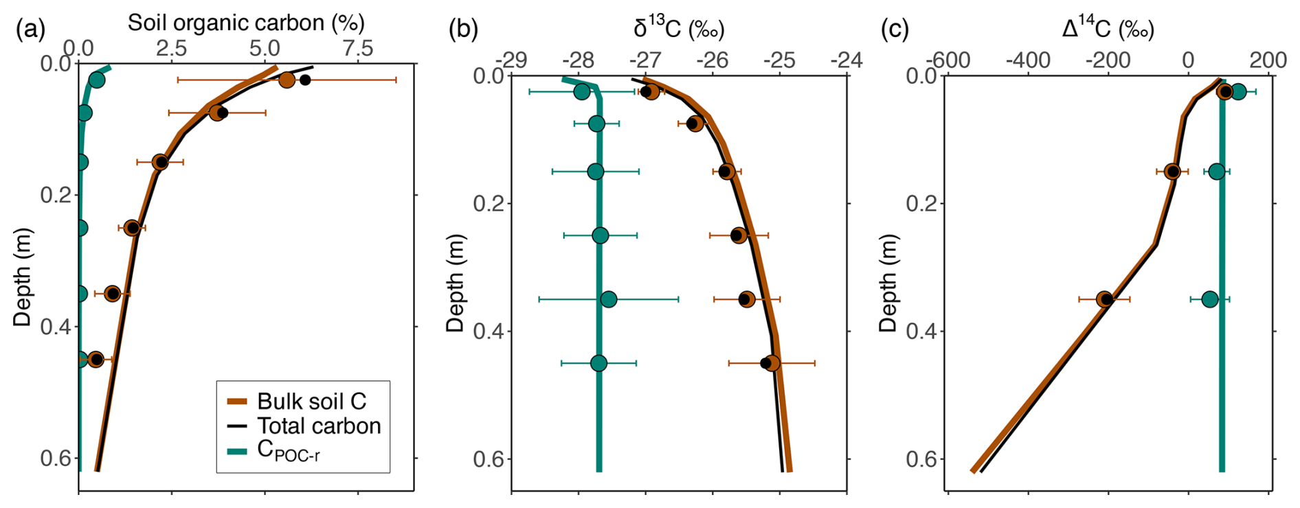
Figure 2 Simulated depth profiles of (a) OC (%), (b) δ¹³C (‰) and (c) Δ¹⁴C (‰) of the POC and bulk SOC pools (i.e. the sum of C_min-b, C_DOC-b and C_mic-b), based on a calibration combining data on OC, δ¹³C and Δ¹⁴C for these pools. Circles indicate measured values for POC (green), mineral-associated OC (brown) and total OC (black) by Schrumpf et al. (2013). Error bars indicate the standard deviation on the measurements of POC and MAOC (when no error bars are visible, the error was smaller than the size of the circles showing the averages).

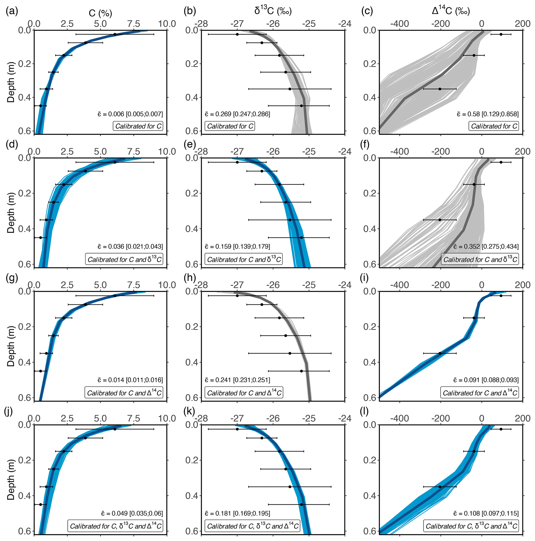
Figure 3 Optimised depth profiles of total OC, δ¹³C and Δ¹⁴C obtained by optimising the model using measurements of the POC and MAOC pools under different calibration scenarios: (1) optimisation using OC data only (a–c); (2) optimisation using OC and δ¹³C data (d–f); (3) optimisation using OC and Δ¹⁴C data (g–i); and (4) optimisation using C, δ¹³C and Δ¹⁴C data (j–l). These simulations show the 10 % best solutions obtained using the DE algorithm. In each row, blue lines show depth profiles that were optimised, while grey lines show simulations of isotopes using the same optimised parameters. Dots and error bars show measured data by Schrumpf et al. (2013). The average error, calculated as a weighted average of the errors for POC and bulk soil OC (squared relative errors; see Sect. 2.3.2), is denoted by $\stackrel{\mathrm{‾}}{\mathit{ϵ}}$, and the inter-quantile range is shown between squared brackets.

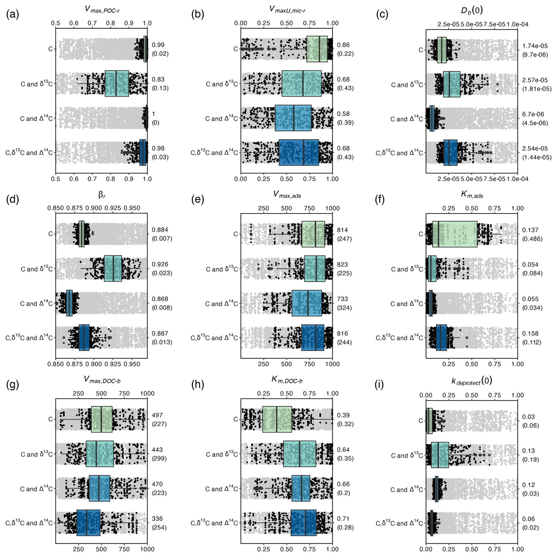
Figure 4 Ranges in parameter values that resulted in the retained model simulations in Fig. 3. The ranges are shown for all optimised parameters, grouped per calibration scenario. Black dots show the retained parameter values, while boxplots show the quantiles of these optimal parameter values. Grey dots show all parameter values tested by the DE algorithm in the range of the retained values. The median and interquartile range (between brackets) of the retained values are shown on the right side of the graphs.

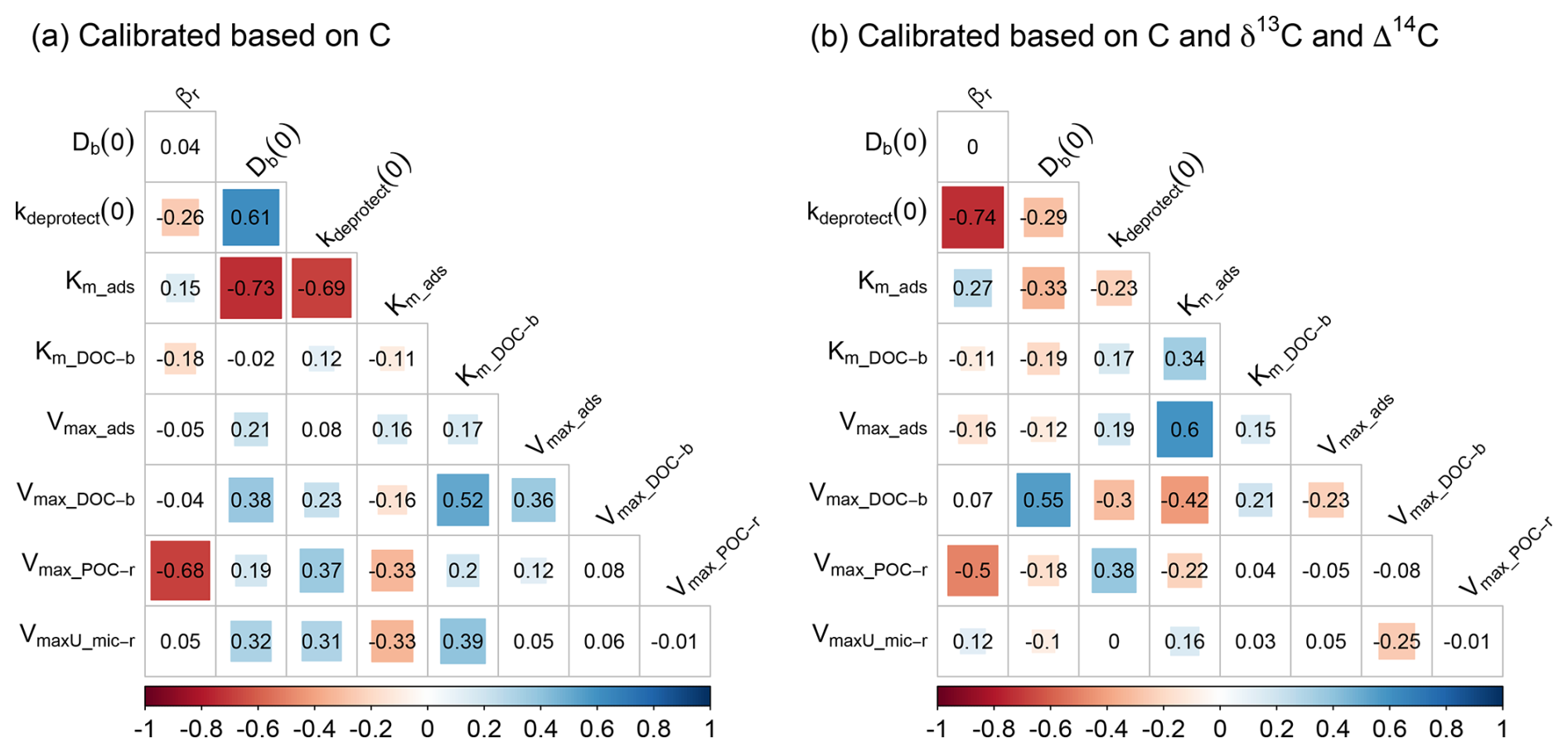
Figure 5 Correlation between the optimised parameters for the calibration scenarios using data on (a) OC only and (b) OC, δ¹³C and Δ¹⁴C. Numbers are the correlation coefficients, while colours are shown for parameter combinations with a significant correlation (p < 0.05). Correlation plots for the other calibration scenarios are shown in Fig. S9.

2.4 Assessment of parameter equifinality

After parameter optimisation using the DE algorithm, the equifinality of the optimised parameters was analysed. Multiple methods are available to this end, such as GLUE (Beven and Binley, 1992) and Bayesian approaches (e.g. Vrugt, 2016), but these methods require prior information on the parameter value distribution to perform optimally. As this information was not available for the optimised parameters, an alternative approach was developed.

The DE algorithm efficiently explores the multi-dimensional parameter space by proposing new sets of parameter combinations during every iteration, based on previously generated parameter sets. To assess if multiple parameter combinations resulted in behavioural models, we kept track of all tested sets of parameter values during the optimisation procedure. For every calibration scenario, this resulted in 54 000 non-unique parameter sets that were generated in the parameter space. In a next step, the model was run using the unique parameter combinations, and the results and respective model errors were stored. The parameter sets resulting in the 10 % lowest errors were retained and were considered to be behavioural models after visually assessing that the model results were within the uncertainty of the measured values (Fig. 3). To assess how the different calibration scenarios influenced model results, the depth profiles of total OC, δ¹³C and Δ¹⁴C were plotted for every calibration scenario (Fig. 3). To assess how each scenario influenced the range in optimal parameter values that resulted in behavioural models, the range of these parameter values for the different calibration scenarios was plotted (Fig. 4). All parameter values explored by the DE algorithm were plotted to confirm that the entire parameter space within the provided boundaries was explored (Fig. 4). Last, to assess correlations between parameters leading to behavioural models, correlation plots for these parameter values were developed using the Pearson correlation coefficient (Fig. 5).

2.5 Sensitivity analysis

2.5.1 Selection of calibration parameters

To assess the influence of the 11 parameters that were initially selected for optimisation (Table S1), a sensitivity analysis was carried out using the PAWN method (Pianosi and Wagener, 2015). This is a density-based global sensitivity analysis that quantifies the model sensitivity related to uncertainties of input parameters based on the cumulative distribution function (CDF) of the output distribution. This is done for the CDF when all parameters are varied (the unconditional CDF) and when one parameter is kept constant (the conditional CDF). The distance between both cumulative distributions is used to quantify the sensitivity of the model to different parameters and is calculated using the Kolmogorov–Smirnov (KS) statistic. The advantage of this method is that it does not assume that the variance in the model output is a measure for model uncertainty, making it more suitable to deal with e.g. multi-modal or skewed distributions than variance-based sensitivity analyses. The parameter sets to calculate the conditional and unconditional CDFs were obtained using the MATLAB^® version of the SAFE toolbox (Pianosi et al., 2015), which was also used to post-process the results and calculate the KS statistic. In addition to the parameters to be tested, a dummy parameter with no influence on the model results was included in the sensitivity analysis. The KS statistic calculated for the dummy parameter was subtracted from the KS statistics of the model parameters before the results were analysed. We used 500 parameter sets to calculate the unconditional CDFs, 500 parameter sets to calculate the conditional CDFs and 50 conditioning values sampled from the one-dimensional space of each tested parameter, following recommendations by Pianosi and Wagener (2015). The parameter values were varied over the range that resulted in the 10 % best solutions in the first round of model optimisation (see Sect. 2.3.2 and Table S1).

2.5.2 Sensitivity of parameters influencing the simulated δ¹³C depth profile

In a second sensitivity analysis, the sensitivity of the shape of the simulated δ¹³C depth profile to five model parameters was tested: (1) the δ¹³C value of OC inputs from aboveground biomass (δ¹³C_leaf), (2) the δ¹³C value of root OC inputs (δ¹³C_root), (3) the δ¹³C of rhizodeposit OC inputs (δ¹³C_exudates), (4) the fraction of microbial biomass derived from soil CO₂ (α) and (5) the change in fractionation against ¹³C by plants per unit change in atmospheric CO₂ concentration (S). The value of these parameters was varied over a range that results in a change in δ¹³C value of 1 ‰ (Table S4) to assure a uniform effect of the parameter ranges on the simulated depth profiles of δ¹³C, except for α, which was varied over the range of values reported in the literature. We note that the process of absorption was not included in this sensitivity analysis, as there is no preferential absorption of ¹²C, ¹³C or ¹⁴C on minerals in the model. The sensitivity of three characteristics of the simulated δ¹³C depth profiles was assessed: (1) the δ¹³C value in the top centimetre of the soil, (2) the δ¹³C value at a depth of 0.40 m and (3) the difference in δ¹³C between these two soil layers. The sensitivity analysis was performed using the PAWN method (Sect. 2.5.1) to calculate the global sensitivity of these parameters. In addition, a local sensitivity analysis was performed by plotting depth profiles of δ¹³C for the range over which these parameters were varied during the global sensitivity analysis with the PAWN method.

3 Results

3.1 Simulation of depth profiles of OC, δ¹³C and Δ¹⁴C using the optimal parameters

Model simulations for the litter and the soil compartments of SOILcarb align well with measurements after parameter optimisation using all available data. The simulated amounts of OC, δ¹³C and Δ¹⁴C in the litter layer closely align with measurements after parameter optimisation based on OC, δ¹³C and Δ¹⁴C data (Fig. S6). In addition, the temporal evolution of δ¹³C and Δ¹⁴C reflects changes in the value of these isotopes of atmospheric CO₂ over the past 150 years.

Similarly for the soil, after parameters are optimised using measurements of depth profiles of OC, δ¹³C and Δ¹⁴C of the POC and MAOC pools, the measurements of both pools are simulated very well by the model (Figs. 2 and S7).

This indicates that the model captures differences in the amount of OC in POC and MAOC, in addition to the residence time of OC in these pools. Concerning simulated depth profiles of δ¹³CO₂ and Δ¹⁴CO₂ along the soil profile (Fig. S8), the model simulated δ¹³CO₂ values ca. 4 ‰ larger compared to available OC, as well as positive Δ¹⁴CO₂ values similar to the Δ¹⁴C available OC, in agreement with general observations (Trumbore, 2000; Cerling et al., 1991).

3.2 Simulation of OC depth profiles using different isotopic constraints

Calibrating the model with an increasing number of constraints (data on SOC, δ¹³C and/or Δ¹⁴C) led to the increasing accuracy of simulated depth profiles of δ¹³C and Δ¹⁴C. The results presented in Fig. 2 show an example of the model using the most optimal parameter set. However, a frequentist model optimisation that tunes model parameters to simulate the average measurements as closely as possible does not account for the fact that multiple parameter sets may result in a solution that is within measurement uncertainty (i.e. behavioural models). This was explored by retaining the parameter sets that led to the 10 % best solutions obtained during the DE optimisation, as these were within the uncertainty of measurements (Fig. 3).

When the model is optimised using only data on the OC percentage (OC%) of POC and MAOC (Fig. 3a–c), simulated depth profiles of OC% show a close fit to measurements ($\stackrel{\mathrm{‾}}{\mathit{ϵ}}$ = 0.006 (unitless); $\stackrel{\mathrm{‾}}{\mathit{ϵ}}$ being the average weighted squared relative error for the POC and bulk SOC pools (i.e. MAOC); see Sect. 2.3.2), while simulated values of δ¹³C along the depth profile are overestimated, most notably in the topsoil ($\stackrel{\mathrm{‾}}{\mathit{ϵ}}$ = 0.269). Simulated Δ¹⁴C values are underestimated for most simulations ($\stackrel{\mathrm{‾}}{\mathit{ϵ}}$ = 0.58), with a large spread in simulated values, indicating that the turnover rate of OC along the soil profile is highly variable in this calibration scenario. For the second calibration scenario, the model was optimised using data on OC% and δ¹³C of POC and MAOC (Fig. 3d–f). Retained model results show a close fit between modelled and measured depth profiles of OC% ($\stackrel{\mathrm{‾}}{\mathit{ϵ}}$ = 0.036) and δ¹³C ($\stackrel{\mathrm{‾}}{\mathit{ϵ}}$ = 0.159). Although simulations of topsoil Δ¹⁴C show a closer fit with measurements compared to an optimisation using OC% data only, the average Δ¹⁴C values of SOC are overestimated below a depth of 0.2 m ($\stackrel{\mathrm{‾}}{\mathit{ϵ}}$ = 0.352). This indicates that including δ¹³C as a calibration constraint is not sufficient to correctly simulate Δ¹⁴C values, and thus turnover rates, of subsoil OC. The latter was only the case when data on Δ¹⁴C were used to constrain model parameters (Fig. 3g–l). Model optimisation using data on OC% and Δ¹⁴C, either with or without data on δ¹³C, resulted in a close fit between modelled and measured values of OC% ($\stackrel{\mathrm{‾}}{\mathit{ϵ}}$ = 0.049 and 0.014 respectively) and both isotopic ratios. It is noted that the simulated δ¹³C depth profiles had a lower error when data on δ¹³C were included as a calibration constraint ($\stackrel{\mathrm{‾}}{\mathit{ϵ}}$ = 0.181) compared to when they were excluded ($\stackrel{\mathrm{‾}}{\mathit{ϵ}}$ = 0.241).

The average error in OC% for the behavioural models was the lowest when only OC% data were used as a calibration constraint ($\stackrel{\mathrm{‾}}{\mathit{ϵ}}$ = 0.006) and highest for the scenario using OC% data combined with δ¹³C and Δ¹⁴C ($\stackrel{\mathrm{‾}}{\mathit{ϵ}}$ = 0.049). In contrast, the overall model error (calculated as the sum of the errors for the simulated depth profiles of OC%, δ¹³C and Δ¹⁴C) was the lowest for the scenario constrained by all available data ($\stackrel{\mathrm{‾}}{\mathit{ϵ}}$ = 0.34), while it was the highest for the optimisation scenario using data on only OC% ($\stackrel{\mathrm{‾}}{\mathit{ϵ}}$ = 0.85). This indicates that while the former optimisation scenario does not result in the overall best fit for the simulated depth profiles of OC%, it results in the best overall model performance, given that processes such as the vertical mixing of aboveground and belowground OC (as shown by the δ¹³C values along the soil profile) and the turnover rate of OC (as shown by the Δ¹⁴C values) are simulated more correctly.

3.3 Parameter equifinality

All model parameters were subject to equifinality for all calibration scenarios; i.e. there was always a range of parameter values that resulted in behavioural models. For the retained behavioural models, it was assessed how including different calibration constraints affected (1) the range and (2) the absolute values of the parameters (Fig. 4). In an ideal situation, the parameter values resulting in behavioural models during a parameter optimisation procedure (1) are correct in their absolute values and (2) do not show a large variation. To evaluate the first condition, it is assumed that the scenario in which parameter values are constrained using data on OC, δ¹³C and Δ¹⁴C resulted in the most reliable parameter values, as this scenario led to the lowest average model error ($\stackrel{\mathrm{‾}}{\mathit{ϵ}}$ = 0.34; Fig. 3) and most reliably simulated the turnover rate of SOC along the soil profile. Similarly, it was assumed that the parameter values of the scenario using data on OC only result in the least reliable parameter values ($\stackrel{\mathrm{‾}}{\mathit{ϵ}}$ = 0.85). To evaluate the second criteria, the interquartile range of the parameter values resulting in behavioural models was calculated (Fig. 4).

Adding data on δ¹³C to the calibration constraints, in addition to data on OC, improved only the value of the intensity of bioturbation (D_b(0)), i.e. resulting in values similar to the values obtained with the optimisation scenario using data on OC, δ¹³C and Δ¹⁴C. As simulated depth profiles of δ¹³C are partly shaped by the mixing of aboveground and belowground OC, it is expected that adding information on the δ¹³C of OC better constrains parameters simulating this process. However, the optimal values of D_b(0), after constraining with OC and δ¹³C, exhibited a substantial range. Adding data on Δ¹⁴C to the calibration constraints, in addition to data on OC, most notably improved the values of k_deprotect(0), as is clear from the better prediction of the Δ¹⁴C value along the soil profile (Fig. 3i). Other parameters had values different from the optimisation using C, δ¹³C and Δ¹⁴C and/or had a substantial variation.

The most notable observation from these results is that for six out of the nine calibrated model parameters (all except K_m,ads, K_m,DOC-b and k_deprotect(0)), including data on OC, δ¹³C and Δ¹⁴C did not result in substantially more constrained parameter values compared to when only data on OC are used (Fig. 4). These parameters regulate the simulated amounts of bio-available OC and DOC, two model pools that could not be explicitly constrained using available data. It thus seems that while adding data on δ¹³C and Δ¹⁴C better constrains parameters related to the turnover of the largest SOC pool (mineral-associated C), it does not help to constrain the size of other model pools, which may compensate for each other to result in a correct amount of simulated total OC.

For all optimisation scenarios, there were significant correlations between the optimised parameter values (as shown by the coloured cells in Figs. 5 and S9). A first reason for the correlations between optimised parameter values is a consequence of the model structure, as parameter values can compensate inputs to and outputs from a model pool so its steady-state size is similar. For example, when only data on OC were used to optimise model parameters (i.e. the optimisation objective was only to get a good fit between measured and modelled OC% of POC and MAOC, irrespective of, for example, the turnover rate of OC), there is a strong correlation (R² = −0.69) between the rate of OC desorption from minerals (k_deprotect(0)) and the affinity of DOC for adsorption (k_{m_ads}; note that lower values of k_m imply a higher affinity). This is to be expected, as low and high rates, respectively, of both OC inputs and outputs to mineral-associated OC will lead to a similar size of this pool, although with respective slow and fast turnover rates. In contrast, when the turnover of the mineral-associated OC pool is included as a calibration criterion (through its Δ¹⁴C value), this correlation is absent, as only a narrow range in desorption rates (k_deprotect(0)) result in the correct turnover rate of this pool (Fig. 4i).

A second reason for such correlations is related to the formulation of the mathematical equations. For example, parameters in the numerator and denominator of an equation may compensate for each other. This is clear from the scenario including most optimisation data (Fig. 5b), where there is strong correlation between V_{max_ads} and K_{m_ads}, which occur in the numerator and denominator, respectively, of the equation representing the rate of DOC adsorption on minerals. While such correlations are generally unwanted (they are an expression of equifinality) and complicate the optimisation procedure, they reflect the ability of the optimisation algorithm to find parameter values that lead to a narrow range of adsorption rates, resulting in the correct simulation of the turnover time of the mineral-associated OC pool.

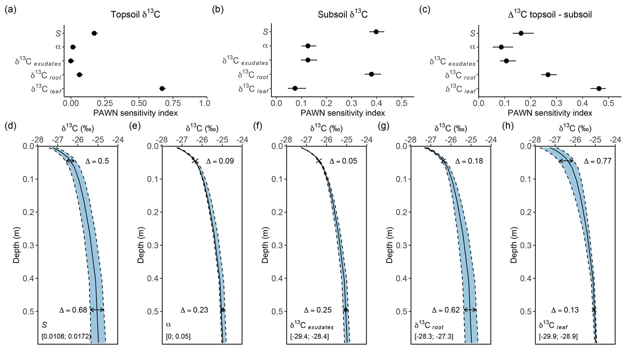
Figure 6 Sensitivity of simulated δ¹³C depth profiles to five model parameters: (1) the change in fractionation against ¹³C by plants per unit change in atmospheric CO₂ concentration (S), (2) the fraction of microbial biomass carbon derived from CO₂ assimilation (α), (3) the δ¹³C of rhizodeposit OC inputs (δ¹³C_exudates), (4) the δ¹³C value of root OC inputs (δ¹³C_root) and (5) the δ¹³C value of leaf OC inputs (δ¹³C_leaf). The sensitivity of these parameters is calculated for topsoil δ¹³C (0.01 m depth), subsoil δ¹³C (0.40 m depth) and the difference in δ¹³C between these layers (Δ¹³C topsoil−subsoil). The top row (a–c) shows the results for the global sensitivity analysis, while the bottom row (d–h) shows the results for the local sensitivity analysis. The Δ values in the lower row indicate the maximum difference in the simulated δ¹³C values for the topsoil and subsoil, while the ranges in the lower-left corners of these graphs show the range over which the respective parameter values were varied.

3.4 Sensitivity of parameters affecting simulated δ¹³C depth profiles

Different model parameters had a distinct effect on the simulated depth profiles of δ¹³C. The global sensitivity analysis of parameters affecting the δ¹³C value of both topsoil and subsoil OC (Fig. 6a–c) showed that the δ¹³C value of topsoil OC was most influenced by the δ¹³C value of leaves, while the other tested parameters had a limited effect. The subsoil (0.40 m depth) δ¹³C was influenced most by the δ¹³C of roots and the effect of atmospheric CO₂ concentration on isotopic fractionation against δ¹³CO₂ during photosynthesis. The influence of the δ¹³C value of leaves on the subsoil δ¹³C was negligible, indicating that the incorporation of aboveground biomass into the soil profile was limited to the uppermost soil layers. The change in the δ¹³C value along the soil profile (Δ¹³C topsoil−subsoil) was most sensitive to the δ¹³C of leaves, the δ¹³C of roots and the effect of atmospheric CO₂ concentration on isotopic fractionation against δ¹³CO₂ during photosynthesis. The local sensitivity analysis (Fig. 6d–h) confirmed these results, showing that the factors having the largest effect on absolute values of δ¹³C along the soil profile were the δ¹³C values of leaves and roots and the effect of atmospheric CO₂ concentration on isotopic fractionation against δ¹³CO₂ during photosynthesis.

4 Discussion

4.1 Simulation of δ¹³C depth profiles in SOILcarb: mechanisms and challenges

During the past decades, multiple mechanisms have been put forward to explain the generally observed increase in the δ¹³C value of SOC with depth in temperate ecosystems. Here, it is assessed to what extent these mechanisms are reflected in the model outcomes. Three main mechanisms that have been proposed are simulated by SOILcarb. The first mechanism concerns inputs of ¹³C-depleted aboveground litter at the soil surface and vertical mixing with ¹³C-enriched belowground inputs along the soil profile (e.g. Wynn et al., 2006; Jagercikova et al., 2017). The sensitivity analysis showed that this mechanism plays an important role in shaping the depth profile of the δ¹³C value of SOC at the studied site (Fig. 6c). This effect played a role down to a depth of ca. 0.3 m, as shown by a model simulation in which the mixing of above- and belowground vegetation was the only mechanism affecting the δ¹³C depth profile (Fig. S10). The second mechanism concerns temporal variations in the δ¹³C value of vegetation and thus OC inputs to the soil (e.g. Paul et al., 2019; Wynn et al., 2006). In SOILcarb, this effect has been partitioned into (1) temporal changes in the δ¹³C value of atmospheric CO₂ (Keeling, 1979) and (2) the effect of atmospheric CO₂ concentration on the discrimination against ¹³CO₂ during photosynthesis (i.e. a higher atmospheric CO₂ concentration leads to more intense fractionation against ¹³CO₂ by plants and thus lower δ¹³C values; Schubert and Jahren, 2012). Additional simulations with SOILcarb show that when only the first mechanism is considered, the simulated δ¹³C of SOC increases by ca. 1 ‰ with depth (Fig. S11). While this process thus contributes substantially to the observed increase in δ¹³C with depth, including the effect of atmospheric CO₂ concentration on fractionation against δ¹³CO₂ during plant photosynthesis was necessary to simulate the measured increase in δ¹³C of ca. 2 ‰ with soil depth (Fig. 2b). The last mechanism is heterotrophic CO₂ assimilation by soil microbes (e.g. Šantrůčková et al., 2018; Nel and Cramer, 2019). The sensitivity analysis showed that this was the mechanism with the lowest impact on the difference in δ¹³C between the topsoil and the subsoil, with the effect on the range in subsoil δ¹³C being 0.23 ‰ when the value of α varied over the range reported in the literature (Fig. 6e). Our model simulations thus suggest that, in contrast to proposals of this mechanism being important based on empirical studies, the potential effect is limited. At the study site, this is caused by the limited amount of CO₂ that is assimilated by soil microbes (1.1 % of total microbial biomass; Akinyede et al., 2020) and the limited difference between the δ¹³C value of SOC and soil CO₂ of 4.4 ‰ (Cerling et al., 1991).

While numerical simulations of depth profiles of δ¹³C help to quantify the importance of different mechanisms shaping the vertical profile, these simulations are prone to uncertainties. For example, the absolute values of the δ¹³C of SOC depend on the δ¹³C value of vegetation (Fig. 6f–h). In the present study, we relied on measurements made at the study site to obtain this information, but these measurements are often not available. Estimating the δ¹³C of vegetation based on literature values when measured data are not available is unlikely to be reliable, as δ¹³C values of C3 vegetation vary over a large range (between ca. −23 ‰ to −32 ‰) depending on, for example, precipitation (Kohn, 2010) and vegetation type (Martinelli et al., 2021). Also the δ¹³C value of different plant organs varies considerably (Bowling et al., 2008). Most notably, estimating the δ¹³C value of root exudates is challenging. Thus, there is considerable uncertainty on estimates of the δ¹³C value of different sources of OC inputs to the soil. Therefore, model users should be aware of large uncertainties in simulated absolute values of the δ¹³C of SOC when measured values are not available and thus balance the benefits of simulating δ¹³C versus the increased uncertainty.

4.2 Overparameterisation and equifinality in soil biogeochemical models

Our results show that overparameterisation, which arises when a numerical model has too many parameters compared to the data available to constrain parameter values, has important consequences for the correct simulation of SOC dynamics. As many of the recently developed SOC models have a similar structure and use similar equations, it is likely that this is a general issue for such models (Sierra et al., 2015; Marschmann et al., 2019), as has previously been shown for conventional turnover-based pool models (Braakhekke et al., 2013; Luo et al., 2016, 2017). Using only data on total OC concentration of the POC and MAOC pools to constrain parameter values resulted in many parameter combinations that led to behavioural models for total OC, i.e. with a close fit to observations. However, simulated Δ¹⁴C values within the soil profile were generally underestimated, while δ¹³C values were slightly overestimated (Fig. 3a–c). This does not confirm our second hypothesis, which anticipated an overestimation of the turnover rate of SOC. Nevertheless, this shows that, if only total SOC stocks are used as the calibration criterion, turnover times of SOC are simulated incorrectly despite a correct simulation of the total SOC inventory. This is important, as a correct simulation of the turnover time of SOC is crucial for making reliable projections of changes in the global C cycle for the coming decades (He et al., 2016; Wang et al., 2019). Similar conclusions were drawn at the plot scale by Braakhekke et al. (2014), who found that the turnover rate for the slowest SOC pool in their model was substantially overestimated without Δ¹⁴C data as a constraint on parameter values. Furthermore, for simulations of the turnover rate of SOC at the global scale, models optimised without data on Δ¹⁴C resulted in a substantial overestimation of the turnover rate of SOC (He et al., 2016). It is thus clear that, without data on the age of SOC as a parameter constraint during calibration, the turnover rate of SOC, especially in the subsoil, is unlikely to be simulated correctly.

Soil biogeochemical models suffer not only from overparameterisation, but also from parameter equifinality, i.e. the phenomenon that multiple parameter sets lead to model results that cannot readily be rejected (Marschmann et al., 2019; Sierra et al., 2015; Tang and Zhuang, 2008). In line with our first hypothesis, a model constrained by data on only SOC stocks was characterised by substantial equifinality (Fig. 3a–c). However, contrary to our third hypothesis, including data on the δ¹³C and/or Δ¹⁴C values of SOC to constrain parameter values during calibration did not substantially reduce the range in most parameter values leading to behavioural models, as shown by the interquartile distances in Fig. 4. Two exceptions were the range in rates of de-protection of OC (k_deprotect(0)) and the affinity of DOC for adsorption (k_m,ads), which were substantially reduced when data on δ¹³C and Δ¹⁴C were included during optimisation.

In line with previous studies, we found that the parameters of the Michaelis–Menten equation (V_max in the numerator and K_m in the denominator) were subject to substantial equifinality (Sierra et al., 2015; Marschmann et al., 2019). The wide use of this equation in microbially driven soil biogeochemical models thus suggests that equifinality of these parameters is common, as information on both the maximum rate (represented by V_max) and the rate-limiting property (represented by K_m) is generally not available. Other parameters of SOILcarb subject to equifinality are representing processes that can compensate for each other to result in a similar total pool size. For example, as shown by the positive correlation between the rate of bioturbation (D_b(0)) and the rate of OC uptake by microbes in the bulk soil (V_max,DOC-b), the more OC in the bulk soil diffuses downwards, the faster microbes need to process it to simulate the measured OC content.

4.3 Ways forward to identify and reduce equifinality in microbially driven SOC models

Sierra et al. (2015) show that equifinality is likely to be an issue in microbially driven SOC models. These authors used the identifiability analysis by Brun et al. (2001) to show that for a relatively simple non-linear microbial model, only two or three parameters could be uniquely identified using calibration data on soil respiration and Δ¹⁴C values of bulk soil and respired CO₂. Similarly, Marschmann et al. (2019) studied five microbially driven SOC models of varying complexity and found substantial equifinality in every model, including a simple two-pool microbial model. From previous studies and the results presented here, it seems that equifinality in soil biogeochemical models can only be partly reduced by including more generally available data, while a reduction in complexity might be needed to fully resolve this issue.

A consequence of equifinality is that it undermines confidence in projected changes in the SOC stock due to environmental changes, as behavioural models can make similar projections for the near future but greatly diverge on a decadal timescale (Luo et al., 2016, 2017). Therefore, identifying and reducing equifinality in soil biogeochemical models is an important prerequisite to increase confidence in the predictions by such models. This is particularly important as these models are incorporated in Earth system models to make predictions of the response of the SOC stock to changes in the Earth's climate (e.g. Wieder et al., 2024) or to assess how changes in agricultural management practices can increase the amount of SOC to mitigate climate change and assign carbon credits (e.g. Mathers et al., 2023).

One way forward to better constrain parameters in microbially driven SOC models is to include additional data during the parameter calibration process. As show in the present and previous studies (He et al., 2016; Wang et al., 2019), the residence time of SOC along the soil profile can be better constrained by including data on Δ¹⁴C during calibration. Reducing the range in acceptable parameter values related to soil microbial dynamics is, however, more challenging, as these data are often lacking, especially for the subsoil or over large spatial scales. Therefore, it is likely that parameters related to soil microbial dynamics in soil biogeochemical models will have to be optimised until more data become available or fixed at values derived from measurements.

Equifinality also implies that it is unlikely that the development of even more complex models will immediately pay off in terms of improved accuracy in predictions. Defining the optimal model structure for simulation and prediction, given the data that are available, is therefore as important as further increasing our process understanding. Multiple methods are available to identify parameter equifinality in environmental models, including the GLUE methodology (Beven and Binley, 1992), Bayesian methods (Vrugt, 2016), the parameter identifiability method from Brun et al. (2001), the Manifold Boundary Approximation Method (Marschmann et al., 2019) and methods to assess local structural parameter identifiability (Stigter et al., 2017), among others (Miao et al., 2011). Many of these methods are easily accessible to researchers in the form of packages in R and other software environments. This should enable modellers to identify this phenomenon in their models and thus reduce model complexity when appropriate.

A last way forward to better constrain model parameters is the construction of integrated databases that bring together data on multiple aspects of the SOM cycle (e.g. OC fractionation, stable and radioisotopes, mineralogy, microbial characteristics, environmental drivers) (Sierra et al., 2015). While in the recent past several efforts have been made to construct global databases with data related to SOC cycling (e.g. ISRAD, Lawrence et al., 2020; WOSIS, Batjes et al., 2020; SoDaH, Wieder et al., 2021; LUCAS, Orgiazzi et al., 2018), the use of these databases to identify and reduce equifinality in soil biogeochemical models has been, surprisingly, very limited. Thus, this is a low-hanging fruit that would significantly increase our confidence in projections of the soil carbon–climate feedback for the coming decades.

5 Conclusions

In this study, a new mechanistic, depth-explicit SOC model (SOILcarb) was presented and used to assess the potential to decrease parameter equifinality by including data on δ¹³C and Δ¹⁴C data of two soil fractions (POC and MAOC) as constraints on parameter values during model optimisation. Our results show that while the optimised model was able to simulate depth profiles of total OC, δ¹³C and Δ¹⁴C in line with measurements, all optimised model parameters were prone to equifinality. Including δ¹³C data, in addition to total OC, did little to improve simulations of the turnover rate of SOC or limit parameter equifinality. Adding Δ¹⁴C data as a calibration constraint, in contrast, resulted in the correct simulation of the turnover rate of SOC, while only substantially reducing equifinality for the parameter regulating the desorption rate of OC from minerals. Adding a combination of δ¹³C and Δ¹⁴C data improved the simulation of the δ¹³C value in the topsoil, the rate of adsorption and desorption of OC on minerals along the soil profile, and thus the turnover rate of SOC along the soil profile. Our results show that more data are needed to reliably constrain parameter values of microbially driven SOC models. As these data are generally not available at larger spatial scales, it is unlikely that including more complexity in soil biogeochemical models will improve simulations in the near future, while more emphasis should be put on finding a better balance between model complexity and available data. This is an important prerequisite to increase confidence in projections of the soil carbon–climate feedback in a world subject to climatic change.