Relationships between the concentration of particulate organic nitrogen and the inherent optical properties of seawater in oceanic surface waters

The concentration of particulate organic nitrogen (PON) in seawater plays a central role in ocean biogeochemistry. The limited availability of PON data obtained directly from in situ sampling methods hinders development of a thorough understanding and characterization of spatiotemporal variability in PON and associated source and sink processes within the global ocean. Measurements of inherent optical properties (IOPs) of seawater, which can be performed over extended temporal and spatial scales from various in situ and remote-sensing platforms, represent a valuable approach to address this gap. We present the analysis of relationships between PON and particulate IOPs, including the absorption coefficients of total particulate matter, a_p(λ); phytoplankton, a_ph(λ); and non-algal particles, a_d(λ), as well as the particulate backscattering coefficient, b_bp(λ). This analysis is based on an extensive field dataset of concurrent measurements of PON and particulate IOPs in the near-surface oceanic waters and shows that reasonably strong relationships hold across a range of diverse oceanic and coastal marine environments. The coefficients a_p(λ) and a_ph(λ) show the best ability to serve as PON proxies over a broad range of PON from open-ocean oligotrophic to coastal waters. The particulate backscattering coefficient can also provide a good proxy for PON in open-ocean environments. The relationships presented here demonstrate a promising means to assess PON from optical measurements conducted from spaceborne and airborne remote-sensing platforms and in situ autonomous platforms. In support of this potential application, we provide the relationships between PON and spectral IOPs at light wavelengths consistent with those used by satellite ocean color sensors.

1 Introduction

Oceanic organic matter consists of dissolved organic matter (DOM) and particulate organic matter (POM) constituents that span a wide range of sizes, from the molecular scale to large particles suspended in water (Verdugo et al., 2004). POM, defined operationally as organic material captured on filters with nominal pore sizes ranging from 0.2 to 0.7 µm, includes large viruses, bacteria, phytoplankton, and zooplankton as well as detrital material (Riley et al., 1971; Eppley et al., 1977, 1983; Morel and Ahn, 1991; Stramski et al., 2004; Kharbush et al., 2020). The elemental composition of the POM pool is made up of, among other constituents, particulate organic carbon, nitrogen, and phosphorus. Despite their important roles in ocean biogeochemistry, observations of mass concentrations of particulate organic carbon (POC), particulate organic nitrogen (PON), and particulate organic phosphorus (POP) obtained from direct measurement methods are relatively scarce, especially in terms of representing extended temporal and spatial scales of variability within the global ocean (Martiny et al., 2013).

To overcome these limitations, the seawater inherent optical properties (IOPs), such as the spectral particulate beam attenuation, c_p(λ); spectral particulate scattering, b_p(λ); spectral particulate backscattering, b_bp(λ); and spectral particulate absorption, a_p(λ), coefficients, measured in situ or estimated from spaceborne remote-sensing platforms using Ocean Color Radiometry (OCR), have been used as proxies for some ocean biogeochemical parameters, including POC and the mass concentration of suspended particulate matter (SPM). All these IOP coefficients are in units of m⁻¹, λ represents the wavelength of light in a vacuum in units of nm, the subscript “p” indicates that the IOP coefficients are associated with suspended particles in water, and the mass concentrations of particulate matter or its organic components are typically expressed in units of mg m⁻³. To the first order, the variability in particulate IOPs is driven by the total concentration of suspended particulate matter as well as the composition and size distribution of suspended particles. Therefore, relationships between particulate IOPs representing the effects of all suspended particles and some measures of concentration of organic particles such as POC exhibit large variations across diverse water bodies within the global ocean because of large changes in the composition and size distribution of particulate matter. For example, large variations have been demonstrated in the relationships between POC and b_p(λ), b_bp(λ), and a_p(λ) across marine environments with highly variable proportions of organic and mineral particulate matter (Woźniak et al., 2010; Reynolds et al., 2016; Koestner et al., 2022; Stramski et al., 2023; Koestner et al., 2024). These studies indicated a need and proposed some approaches to account for variations in particulate composition when particulate IOPs are intended to be used as proxies for POC, especially when a wide range of aquatic environments with highly variable characteristics of particulate assemblages is considered.

Notwithstanding these challenges, many studies in the past have used in situ measurements conducted in different geographically restricted regions of the global ocean to demonstrate that the relationships between POC and particulate IOPs can be reasonably good under conditions that are regionally or environmentally constrained in terms of ocean bio-optical properties. For example, such relationships were examined between POC and c_p(λ) (e.g., Marra et al., 1995; Loisel and Morel, 1998; Bishop, 1999; Claustre et al., 1999; Stramska and Stramski, 2005; Gardner et al., 2006; Bishop and Wood, 2008; Cetinić et al., 2012), between POC and b_bp(λ) (e.g., Stramski et al., 1999, 2008; Allison et al., 2010; Loisel et al., 2011; Cetinić et al., 2012; Kheireddine et al., 2020; Qiu et al., 2021; Barbieux et al., 2022), and between POC and a_p(λ) (e.g., Woźniak et al., 2011; Rasse et al., 2017). While recognizing that single empirical relationships for estimating POC from particulate IOPs are expected to work best if they are region-specific or formulated over a restricted range of marine bio-optical environments, it is also reasonable to assume that such relationships can be useful for application across vast areas of open-ocean pelagic environments because the variations in particulate characteristics in these environments are expected to be constrained to a significant degree compared to the variations observed across all diverse water bodies. For example, these relationships have been used to assess carbon community production from in situ c_p(λ) or b_bp(λ) measurements in the tropical Pacific (Claustre et al., 1999), the South Pacific Gyre (Claustre et al., 2008), and the Mediterranean Sea (Loisel et al., 2011; Barbieux et al., 2022). Vertical fluxes of POC have been described and quantified using POC vs. b_bp relationships applied to in situ b_bp(λ) measurements acquired from autonomous platforms during a subpolar North Atlantic spring bloom (Briggs et al., 2011) and in the Red Sea (Kheireddine et al., 2020). Based on the POC vs. b_bp(λ) relationships, ocean color algorithms have also been developed (e.g., Stramski et al., 1999; Loisel et al., 2001a, 2002; Stramska and Stramski, 2005; Allison et al., 2010; Duforêt-Gaurier et al., 2010) to enhance the abilities of and complement other algorithms that have been used for estimating POC in surface waters of the global ocean from satellite ocean color observations (Stramski et al., 2008, 2022).

Considering the interest in developing an ability to estimate PON from optical measurements along with the existing algorithms that allow the estimation of POC from optical measurements, it is relevant to comment on the canonical Redfield ratio, which describes a consistent atomic ratio of carbon, C; nitrogen, N; and phosphorus, P, in marine plankton, namely $\mathrm{C}:\mathrm{N}:\mathrm{P}$ of $\mathrm{106}:\mathrm{16}:\mathrm{1}$ (Redfield, 1934; Redfield et al., 1963). This ratio could potentially serve as a means to estimate PON from POC. However, it is well recognized that the $\mathrm{C}:\mathrm{N}:\mathrm{P}$ ratios for natural particulate organic matter can vary considerably in the ocean and thus deviate from the canonical Redfield ratio (Copin-Montegut and Copin-Montegut, 1983; Diaz et al., 2001; Körtzinger et al., 2001; Geider and La Roche, 2002; Weber and Deutsch, 2010; White et al., 2006). For example, strong latitudinal patterns in these elemental ratios of marine plankton and particulate organic matter, including nonliving particles such as detritus generated from the decay of phytoplankton cells and zooplankton grazing activity, have been documented (Martiny et al., 2013). Therefore, the subject of estimating PON from optical measurements requires separate dedicated studies, and this paper is a contribution to this line of research.

Recently, a reasonably good relationship between PON and b_bp has been demonstrated based on field measurements made in oligotrophic waters of the western tropical South Pacific (Fumenia et al., 2020). Furthermore, this study used the b_bp measurements from Biogeochemical-Argo (BGC-Argo) floats to quantify new production of phytoplankton biomass that was likely related to intense biological nitrogen (N₂) fixation in this tropical oceanic environment. It is worth noting that at the scale of the global ocean, biological N₂ fixation is a major source of new nitrogen in the euphotic layer, followed by atmospheric and terrestrial deposition (Dugdale et al., 1961; Karl et al., 2002; Capone et al., 2005). Also, different models utilizing a combination of in situ PON measurements and satellite ocean color observations, including satellite-derived ocean remote-sensing reflectance, R_rs(λ), as well as satellite-derived IOPs such as b_bp(λ) and the total absorption coefficient of seawater, a(λ), have been developed for application at the global oceanic scale (Wang et al., 2022). Although the study of Wang et al. (2022) suggests that PON can be estimated from satellite ocean color products, the PON vs. IOP relationships have not yet been investigated using field measurements collected over a broad range of oceanic and coastal marine environments.

The main objective of the present study is to examine the relationships between the PON and particulate IOPs, including b_bp(λ), a_p(λ), a_ph(λ), and a_d(λ), from in situ near-surface measurements collected over a broad range of marine bio-optical environments. For this purpose, we assembled datasets of concurrent PON and IOP measurements from the open-ocean pelagic environments, Arctic seas, and coastal waters around Europe. The relationships between PON and spectral IOPs are presented and discussed in terms of variability and its sources, as observed in the relationships examined across the different marine environments. This analysis provides insights into the potential applicability of different particulate IOPs to serve as proxies for PON.

Table 1 The values of the minimum-to-maximum range (in brackets) and median (in parentheses) for the whole dataset (WD) and for the different subsets of data used in this study. The data subsets are OOD (open-ocean dataset), AOD (Arctic Ocean dataset), and CWD (coastal-water dataset). The results are also shown for the three oceanic regions that are a part of OOD. N_POM is the number of PON or POC measurements. N_bbp is the number of concurrent PON and b_bp(555) measurements. N_ap is the number of concurrent PON and a_p(510), a_ph(510), and a_d(442) measurements.

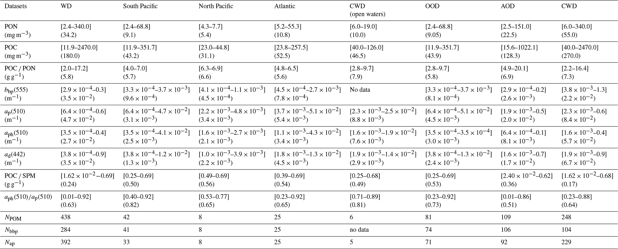
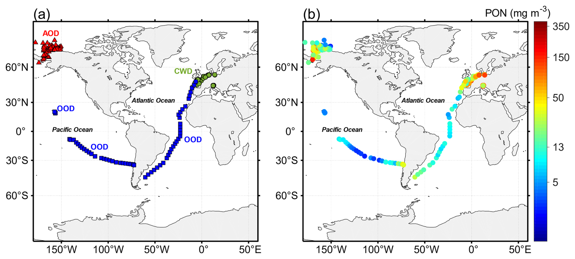
Figure 1 (a) Geographical locations of oceanographic stations shown as color-coded symbols according to the three subsets of data from different oceanic regions. OOD (open-ocean dataset, blue squares), AOD (Arctic Ocean dataset, red triangles), and CWD (coastal-water dataset, green circles) refer to the datasets for the open-ocean Pacific and Atlantic waters, western Arctic seas, and European coastal waters, respectively. (b) Near-surface PON measured at all stations in the whole dataset (WD).

2 Materials and methods

2.1 Geographic locations of in situ measurements

A dataset of in situ biogeochemical and optical measurements was assembled from multiple field experiments performed in various open-ocean and coastal regions covering a broad range of PON, POC, and particulate IOPs collected at depths between the sea surface and 10 m (Fig. 1; Table 1). The whole dataset (referred to as WD) consists of three subsets of data collected in different regions that generally represent different marine bio-optical environments.

The first subset of data (referred to as OOD for the open-ocean dataset) includes measurements made during three cruises conducted in open-ocean waters in the Pacific and Atlantic oceans. The BIOSOPE (Biogeochemistry and Optics South Pacific Experiment) cruise took place from October to December 2004 in the eastern South Pacific Ocean along an east-to-west transect from the Marquesas Islands to the coast of Chile (Claustre et al., 2008; Stramski et al., 2008). The KM12-10 cruise was carried out in June 2012 in tropical waters off the Hawaiian Islands (Johnsen et al., 2014; Reynolds and Stramski, 2021). The ANTXXVI/4 cruise was conducted in April and May 2010 along a south-to-north transect in the Atlantic Ocean between Chile and Germany (Uitz et al., 2015).

The second subset of data (referred to as AOD for the Arctic Ocean dataset) includes measurements collected in the western Arctic seas, specifically in the Chukchi Sea and western Beaufort Sea, during three cruises, HLY1001 in June–July 2010, HLY1101 in June–July 2011, and MR17-05C in August–September 2017 (Arrigo, 2015; Reynolds and Stramski, 2019; Shiozaki et al., 2019). The data collected in these high-latitude environments are characterized by the presence of specific phytoplankton communities and a relatively high contribution of chromophoric dissolved organic matter (CDOM) and non-algal particulate matter to the IOPs of seawater (Reynolds and Stramski, 2019).

The third subset of data (referred to as CWD for the coastal-water dataset) consists of data collected as part of the COASTlOOC (Coastal Surveillance Through Observation of Ocean Color) research project, which involved numerous experiments in various coastal waters around Europe in 1997 and 1998 (Massicotte et al., 2023a). This dataset represents the bio-optical variability encountered across diverse coastal waters, including shelf and relatively shallow environments in the Baltic Sea, North Sea, Wadden Sea, English Channel, and Adriatic Sea, as well as waters affected by many river plumes around Europe (Babin et al., 2003a, b). A small fraction of CWD (<3 % of COASTlOOC data) includes measurements collected in open-ocean waters in the Atlantic Ocean between the Bay of Biscay and the Canary Islands and off the shelf in the Mediterranean Sea, where the bio-optical variability is expected to be driven primarily by phytoplankton and associated material.

The total number of concurrent POC and PON measurements, N_POM, in the whole dataset, WD, is 432 (Table 1). The contributions of OOD, AOD, and CWD to this total number are 18.5 %, 24.9 %, and 56.6 %, respectively. These measurements of PON and POC are used to discuss the variability in the POC $/$ PON ratio in Sect. 3.1. The number of concurrent measurements of PON and IOPs that are used to examine the relationships between these variables is smaller than N_POM. Specifically, the relationship between PON and the backscattering coefficient b_bp presented here is based on 284 measurements in the whole dataset, WD (Sect. 3.2.1), and the relationships between PON and the absorption coefficients, a_p, a_ph, and a_d, are based on 392 measurements (Sect. 3.2.2).

2.2 Measurement methods

The measurement and data processing protocols are described in detail in the references cited in Sect. 2.1. Here we provide a brief summary. Samples for POC and PON determination were collected by filtration of seawater through pre-combusted 25 mm Whatman GF/F filters. After filtration, the samples were transferred into glass vials, dried at 55 °C, and stored until post-cruise analysis. The mass of particulate organic carbon and nitrogen on the sample filters was determined by high-temperature combustion via standard carbon–hydrogen–nitrogen (CHN) analysis following the JGOFS (Joint Global Ocean Flux Study) protocols (Knap et al., 1996). The samples were acid-treated prior to the CHN analysis to remove inorganic carbon. The mass concentration of suspended particulate matter (SPM) was determined gravimetrically by measuring the dry mass of particles collected on GF/F filters. The filters were pre-rinsed, pre-combusted, and pre-weighed using a protocol described in Van der Linde (1998). More details on the methodology of CHN analysis and SPM determinations are provided in Babin et al. (2003a), Reynolds et al. (2016), and Stramski et al. (2008).

The spectral particulate absorption coefficient, a_p(λ), was determined from samples collected on 25 mm GF/F filters using a spectrophotometric filter-pad method. The a_p(λ) spectra included in OOD and AOD were measured mostly with a PerkinElmer Lambda 18 spectrophotometer equipped with a 15 cm integrating sphere using the inside integrating sphere (IS) configuration of measurement, which is considered to provide the best accuracy of measurements when using a filter-pad method (Stramski et al., 2015; Roesler et al., 2018). The exception is the absorption data from the BIOSOPE cruise, which were measured with a PerkinElmer Lambda 19 equipped with a 6 cm integrating sphere using a transmittance (T) configuration of measurement (Bricaud et al., 2010). The non-algal particulate absorption coefficient, a_d(λ), was also determined using the spectrophotometric filter-pad method after the extraction of pigments (associated primarily with phytoplankton) in methanol (Kishino et al., 1985). All absorption data in OOD and AOD were acquired between 300 and 800 nm with a 1 nm step. The a_p(λ) spectra included in CWD were determined from the transmittance–reflectance (T–R) configuration of the filter-pad method in the spectral range of 380–750 nm at 1 nm intervals (Babin et al., 2003b). In this dataset, a_d(λ) was determined by pigment bleaching with sodium hypochlorite (Ferrari and Tassan, 1999). For all absorption samples considered in this study, the spectral phytoplankton absorption coefficient, a_ph(λ), was obtained by subtracting the measured a_d(λ) from the measured a_p(λ). More details on the absorption measurement methodology used in our dataset are provided in Babin et al. (2003b), Bricaud et al. (2010), Uitz et al. (2015), and Reynolds and Stramski (2019).

The spectral backscattering coefficient, b_b(λ), which is the sum of particulate, b_bp(λ), and pure seawater, b_bw(λ), contributions, was calculated from the scattering measurements at a specified backscattering angle (around 140°). After subtraction of b_bw(λ) from b_b(λ), the result was converted to b_bp(λ), assuming a coefficient of proportionality between b_bp(λ) and the scattering at 140°. The backscattering measurements for OOD and AOD were all performed with HydroScat-6 (HOBI Labs, Inc.) instruments providing 6 wavelengths (420, 442, 470, 510, 555, 589 nm) during the BIOSOPE cruise and 11 wavelengths (394, 420, 442, 510, 532, 550, 589, 620, 640, 671, 730, 852 nm) during the HLY1001, HLY1101, MR17-05C, ANTXXVI/4, and KM12-10 cruises. A more detailed description of the procedure to estimate b_bp(λ) from HydroScat-6 measurements is provided in Stramski et al. (2008) and Reynolds et al. (2016).

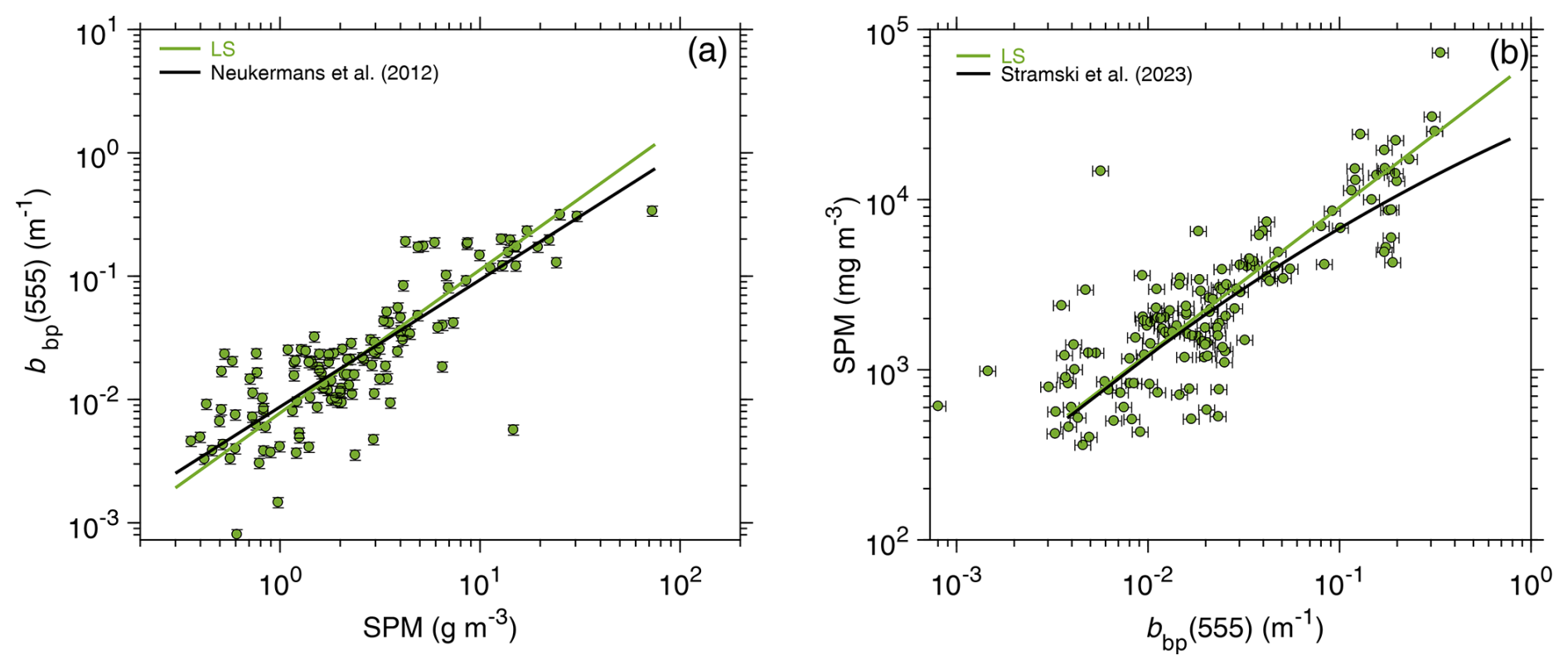
Figure 2 (a) Scatterplot of b_bp(555) as a function of SPM for CWD, where b_bp(555) is estimated from the model of Loisel and Stramski (2000) (referred to as LS model, green circles). The green line refers to the Model-II best linear fit using the log-transformed variables. For comparison, the b_bp(555) vs. SPM relationship of Neukermans et al. (2012), originally developed at 660 nm and recalculated for 555 nm assuming that b_bp(λ) has a mean spectral dependency of λ^−0.5 (Babin et al., 2003a), is also shown (black line). (b) Same as (a) but for SPM as a function of b_bp(555) for CWD. For comparison, the SPM vs. b_bp(555) relationship of Stramski et al. (2023) is also shown (black line). The error bars show the expected uncertainties (±9.5 %) associated with the estimation of b_bp(555) from the LS model (Loisel et al., 2001b).

No in situ measurements of b_bp(λ) were performed during the COASTlOOC experiments. However, in situ measurements of downwelling, E_d(z, λ), and upwelling, E_u(z, λ), irradiances were conducted within the surface ocean layer at each station (where z is depth). From these vertical profiles, the irradiance reflectance just beneath the sea surface, R(0⁻, λ)=E_u(0⁻, $\mathit{\lambda })/E_{\mathrm{d}}$(0⁻, λ), and the average attenuation coefficient for downwelling irradiance, $<K_{\mathrm{d}}\left(\mathit{\lambda }\right){>}_{\mathrm{1}}=\mathrm{1}/z_{\mathrm{1}}$, between the surface and the first attenuation depth was calculated (0⁻ indicates the depth just beneath the sea surface, and z₁ is the first attenuation depth at which the downwelling irradiance is reduced to about 36.8 % of its surface value). For CWD, b_bp(λ) was then estimated from the LS inverse optical model, which uses R(0⁻, λ), <K_d(λ)>₁, and the sun angle as input parameters (Loisel and Stramski, 2000). As b_bp(λ) is driven largely by the concentration of suspended particulate matter, SPM, the reliability of LS-derived b_bp(λ) was assessed through the comparison with b_bp(555) obtained from a previously developed empirical relationship (Neukermans et al., 2012) between b_bp and SPM (Fig. 2a). The same intercomparison exercise was performed using the empirical relationship between SPM and b_bp(555) (Fig. 2b) developed by Stramski et al. (2023). This comparative analysis supports the use of LS-derived b_bp(λ) for the COASTlOOC experiments considered in this study (Fig. 2). We note that similar support was obtained with the use of the LS2 model (Loisel et al., 2018) instead of the LS model (not shown), where the main difference is that the application of LS2 model requires the input of remote-sensing reflectance, R_rs(λ), rather than R(0⁻, λ).

The measurements of PON, POC, and IOPs are subject to errors that are not amenable to straightforward quantification, especially on a sample-by-sample basis. Multiple factors related to measurement methodology, instrumentation, environmental conditions, and no knowledge of true values make it challenging to determine the errors. It is common to use a series of replicate observations for evaluating one of the components of measurement uncertainty. The precision of POC and PON measurements performed during the BIOSOPE cruise has been determined from the analysis of duplicate and triplicate samples. The coefficient of variation (CV) was, on average, about 8.7 % and 7.7 % for POC and PON, respectively (Stramski et al., 2008). For the different cruises comprising AOD, the median coefficient of variation for replicate samples of POC varied between about 2 % and 5 % (Stramski et al., 2023), and a similar range of 3 % to 4 % was observed for PON. For the COASTlOOC experiment, the CV values were 3.7 % and 6.8 % for POC and PON, respectively (Ferrari et al., 2003). Thus, the precision of POC and PON measurements is expected to typically remain below 10 %. Regarding the particulate absorption measurements, the lowest uncertainties below 10 %, with high precision typically of a few percent, are expected for the IS configuration of the filter-pad method, and the highest uncertainties are expected for the T configuration of this method (Stramski et al., 2015; Roesler et al., 2018). While most absorption data in the OOD and AOD were obtained using the IS method, the T method was used during the BIOSOPE cruise, for which the uncertainty in a_p(λ) was estimated at about 15 %, while the precision based on replicate samples was at a few percent in the visible spectral range (Bricaud et al., 2010). For the T–R method used during the COASTlOOC experiment, the uncertainties are expected to be in between those for the IS and T methods (Stramski et al., 2015). Earlier analysis of situ determinations of the backscattering coefficient indicated that the uncertainty estimates commonly fall in the 10 %–20 % range (e.g., Berthon et al., 2007; Doxaran et al., 2016) but can be reduced to a few percent under certain circumstances (Sullivan et al., 2013).

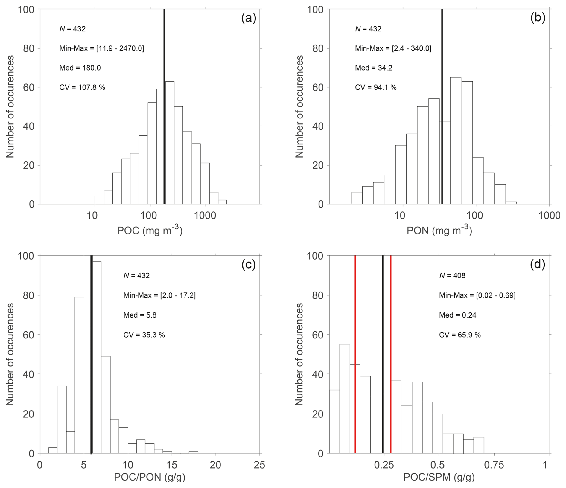
Figure 3 Frequency distribution of near-surface values of (a) POC, (b) PON, (c) POC $/$ PON (g g⁻¹, i.e., gram/gram basis), and (d) POC $/$ SPM (g g⁻¹) for the whole dataset (WD) used in this study. The vertical solid black lines correspond to the median values. The vertical red lines in panel (d) refer to the threshold values of POC $/$ SPM of 0.12 and 0.28, which delimit the mineral-dominated, mixed, and organic-dominated particulate assemblages (Stramski et al., 2023). The minimum-to-maximum range (Min–Max), median (Med), and coefficient of variation (CV) are also indicated. N is the number of data points.

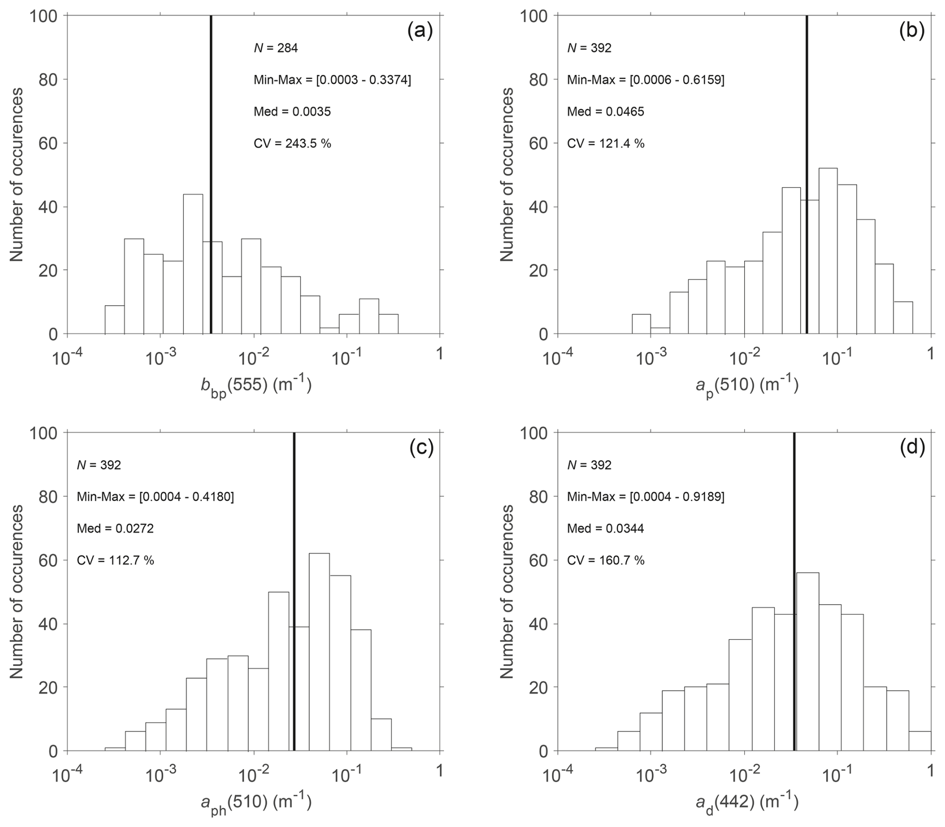
Figure 4 Frequency distribution of the near-surface values of (a) b_bp(555), (b) a_p(510), (c) a_ph(510), and (d) a_d(442) for the whole dataset (WD) used in this study. The vertical solid black lines correspond to the median values. The minimum-to-maximum range (Min–Max), median (Med), and coefficient of variation (CV) are indicated. N is the number of data points.

2.3 Description of the dataset

The biogeochemical and optical properties exhibit a large variability in our whole dataset (WD), which is associated with a range of diverse marine bio-optical and trophic conditions in this dataset (Figs. 3 and 4 and Table 1). Overall, PON (Fig. 3a) and POC (Fig. 3b) range over 2 orders of magnitude, from 2.4 to 340.0 and 11.9 to 2470.0 mg m⁻³, respectively. Minimum concentrations of these particulate organic pools are found in the subset of open-ocean data (OOD), with the smallest values of PON and POC observed in the oligotrophic waters of subtropical gyres in the Pacific and Atlantic oceans (Table 1). The OOD is also characterized by the highest median value of POC $/$ SPM = 0.53 (Table 1), which is indicative of highly organic-dominated particulate assemblages. Maximum values of PON and POC are found in the COASTlOOC subset of data (CWD), which also has the lowest median value of POC $/$ SPM = 0.17 (Table 1). This indicates that the coastal waters in the CWD generally have a significantly smaller contribution of organic particles to SPM compared with the two other subsets of data (OOD and AOD). The median values of PON and POC in the European coastal environments are about 5 to 10 times higher than those in the Pacific and Atlantic oceans and twice as high as in the western Arctic seas (Table 1). Generally, the median values of biogeochemical variables in the Arctic dataset are between those in the open-ocean and coastal-water datasets. The range of variation in PON and POC is largest (about 60-fold) in the CWD and AOD, whereas OOD has about 30-fold range of variation. The median value of POC $/$ PON is 5.8 g g⁻¹ (grams per gram) (≈6.8 mol mol⁻¹) for the whole dataset, which is very similar to the canonical molar Redfield ratio of 6.6 mol mol⁻¹. However, the POC $/$ PON ratio exhibits a large range of variability (2.0–17.2 g g⁻¹) in our dataset (Fig. 3c, more details in Sect. 3.1).

The POC $/$ SPM ratio expressed on a g g⁻¹ basis (Fig. 3d) can be used as a proxy for characterizing the contributions of organic vs. inorganic particles to SPM. Some threshold values have been proposed to delimit the organic-dominated, mixed, and mineral-dominated particulate assemblages in previous studies (Woźniak et al., 2010; Lubac and Loisel, 2007; Loisel et al., 2023; Stramski et al., 2023). The threshold values established in different studies are similar; for example, Stramski et al. (2023) proposed POC $/$ SPM = 0.12 as a boundary between the mineral-dominated and mixed particulate assemblages and POC $/$ SPM = 0.28 as a boundary between the mixed and organic-dominated assemblages. Using these threshold values, we determined that 43.9 % of our whole dataset is associated with organic-dominated particulate assemblages, 27.4 % with mineral-dominated assemblages, and 28.7 % with mixed assemblages.

Similar to the biogeochemical parameters, the particulate IOPs exhibit a large range of variability, which is illustrated in Fig. 4 for the optical coefficients at selected light wavelengths. As expected, the IOP values are generally higher in the turbid coastal waters included in CWD and smaller in the subtropical gyres included in OOD (Table 1). The median value of b_bp(555) in the European coastal environments (CWD) is 1 order of magnitude higher than in the western Arctic seas (AOD) and 2 orders of magnitude higher than in the open-ocean waters of the Pacific and Atlantic oceans (OOD). The median values of a_p(510), a_ph(510), and a_d(442) in the CWD are similar to those in the AOD but are 1 order of magnitude higher than those in the OOD (Table 1). The $a_{\mathrm{ph}}\left(\mathrm{510}\right)/a_{\mathrm{p}}\left(\mathrm{510}\right)$ ratio, which quantifies the proportion of phytoplankton absorption to the total particulate absorption at a light wavelength of 510 nm, varies by a factor of 83 within the whole dataset (see WD in Table 1). Very high variability in this parameter is observed in the Arctic dataset (a factor of 78), whereas the variation in the open-ocean and coastal-water datasets is much smaller (about four-fold).

2.4 Statistical indicators

Model-I linear regression can be considered a valid approach when the primary goal of the analysis is to fit a predictive model to a dataset of the response (y) and explanatory (x) variables, i.e., to reduce variance in prediction of y from x (Legendre and Michaud, 1999; Sokal and Rohlf, 1995). In this study, the analysis of PON (response variable) vs. IOPs (explanatory variables) is aimed at establishing the predictive relationships. An alternative linear regression analysis is Model II, which typically serves to quantify the strength of the linear relationship between the examined variables but can also be an adequate option for predictive purposes, especially when both variables are subject to error and the error in data of x is not significantly smaller than the error in data of y (McArdle, 1988). In our study, the uncertainties in the explanatory variables (IOPs) are not necessarily much smaller than those in PON (see Sect. 2.2), so we tested both the Model-I and Model-II regressions. Specifically, we evaluated (i) the ordinary least squares Model-I linear regression, (ii) the robust least squares Model-I linear regression, and (iii) the Model-II linear regression using the major-axis method (Kermack and Haldane, 1950; York, 1966). These regression models were applied to the log₁₀-transformed PON and IOP data. It should be noted that the Model-II linear regression using the major-axis method is appropriate when both variables are expressed in the same physical units or are dimensionless (e.g., log-transformed variables) (Legendre and Legendre, 2012).

This analysis was made for the whole dataset, WD, and for the three data subsets, OOD, AOD, and CWD. From this analysis we obtained the best-fit equations in the form of a power function and the coefficient of determination (R²) between the log₁₀-transformed variables. The general formula of the power function is

$$\begin{array}{}\text{(1)}& \text{PON}=A\text{ IOP}(\mathit{\lambda }{)}^B,\end{array}$$

where IOP(λ) represents one of the spectral particulate IOPs; A and B are the best-fit coefficients; and the PON and IOP(λ) variables are expressed in units of mg m⁻³ and m⁻¹, respectively. For most cases examined, the general pattern of data points of PON vs. IOP is consistent with a power function; however, there is an exception for the relationship of PON vs. b_bp(λ) for the whole dataset, WD. In this case, we also used a third-degree polynomial function that provided a better fit to the data than the power function.

Table 2 Statistical metrics used in the evaluation of the goodness-of-fit of algorithmic formulas.

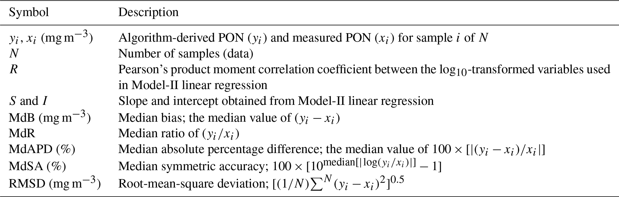
To compare the three methods of regression analysis, we examined the goodness-of-fit of each regression equation (i.e., each PON algorithm utilizing a given particulate IOP as input to the algorithm) through the analysis of algorithm-derived PON vs. measured PON using the algorithm development dataset. This evaluation involved the use of Model-II linear regression based on the major-axis method applied to data of algorithm-derived vs. measured PON, as well as the calculation of several statistical metrics that quantify differences between the algorithm-derived and measured values of PON (Table 2). These statistics include the slope (S) and the intercept (I) obtained from the Model-II linear regression applied to log₁₀-transformed variables of algorithm-derived vs. measured PON. These parameters are useful to reveal the potential presence of bias across the dynamic range of PON. The median bias (MdB) and the median ratio (MdR) quantify the aggregate systematic deviations between the (non-transformed) algorithm-derived and measured values of PON for the dataset investigated. The median absolute percentage difference (MdAPD) and the root-mean-square deviation (RMSD) characterize random deviations between the algorithm-derived and measured PON. We also use the median symmetric accuracy (MdSA), which can be interpreted similarly to MdAPD as a median percentage difference, but, unlike MdAPD, MdSA does not penalize over- and underprediction differently (Morley et al., 2018).

The comparative analysis of algorithm-derived PON vs. measured PON indicated that some statistics are better for the predictive regression formulas obtained from the Model-II regression compared with the predictive formulas obtained from the Model-I regression analysis. Specifically, this improvement was observed for the slope (S) and the intercept (I) of the log-transformed algorithm-derived PON vs. measured PON. Other statistics did not reveal any advantage to using Model-II over Model-I regression (or vice versa) for establishing the empirical algorithms for PON vs. IOPs. As a result of this analysis, in the remainder of this study, all PON vs. IOP algorithms presented are based on the Model-II regression using the major-axis method applied to the log₁₀-transformed variables.

For the final algorithms based on the Model-II regression analysis, we further evaluated the relationships between the algorithm-derived and measured PON using the radar charts (Tran et al., 2019). For this purpose, MdB, MdAPD, MdSA, RMSD, S, and R were normalized as follows:

$$\begin{array}{c}{\displaystyle }{\mathrm{MdB}}_{\mathrm{norm}}\left(j\right)={\displaystyle \frac{\left|\text{MdB}\left(j\right)\right|}{\max (\left|\text{MdB}\left(j\right)\right|,j=\mathrm{1},k)}}\\ {\displaystyle }{\mathrm{MdAPD}}_{\mathrm{norm}}\left(j\right)={\displaystyle \frac{\text{MdAPD}\left(j\right)}{\max (\text{MdAPD}\left(j\right),j=\mathrm{1},k)}}\\ {\displaystyle }{\mathrm{MdSA}}_{\mathrm{norm}}\left(j\right)={\displaystyle \frac{\text{MdSA}\left(j\right)}{\max (\text{MdSA}\left(j\right),j=\mathrm{1},k)}}\\ {\displaystyle }{\mathrm{RMSD}}_{\mathrm{norm}}\left(j\right)={\displaystyle \frac{\text{RMSD}\left(j\right)}{\max (\text{RMSD}\left(j\right),j=\mathrm{1},k)}}\\ {\displaystyle }{S}_{\mathrm{norm}}\left(j\right)={\displaystyle \frac{\left|\mathrm{1}-S\left(j\right)\right|}{\max (\left|\mathrm{1}-S\left(j\right)\right|,j=\mathrm{1},k)}}\\ {\displaystyle }{R}_{\mathrm{norm}}\left(j\right)={\displaystyle \frac{\min (R\left(j\right),j=\mathrm{1},k)}{\mathrm{R}\left(\mathrm{j}\right)}},\end{array}$$

where j represents each individual PON algorithm based on a given IOP and k is the number of tested algorithms. In addition, to facilitate the comparison between the goodness-of-fit of PON algorithms based on different IOPs, the area associated with the polygons linking the normalized statistical indicators was computed as

$$\begin{array}{rl}\text{Area}& ={\displaystyle \frac{\mathrm{1}}{\mathrm{2}}}\times {\displaystyle \frac{\mathit{\pi }}{\mathrm{6}}}\times [{\mathrm{RMSD}}_{\mathrm{norm}}\left(j\right)\times {\mathrm{MdAPD}}_{\mathrm{norm}}\left(j\right)\\ & +{\mathrm{MdAPD}}_{\mathrm{norm}}\left(j\right)\times {\mathrm{MdSA}}_{\mathrm{norm}}\left(j\right)\\ & +{\mathrm{MdSA}}_{\mathrm{norm}}\left(j\right)\times {\mathrm{MdB}}_{\mathrm{norm}}\left(j\right)+{\mathrm{MdB}}_{\mathrm{norm}}\left(j\right)\\ & \times S_{\mathrm{norm}}\left(j\right)+S_{\mathrm{norm}}\left(j\right)\times R_{\mathrm{norm}}\left(j\right)\\ & +R_{\mathrm{norm}}\left(j\right)\times {\mathrm{RMSD}}_{\mathrm{norm}}\left(j\right)].\end{array}$$

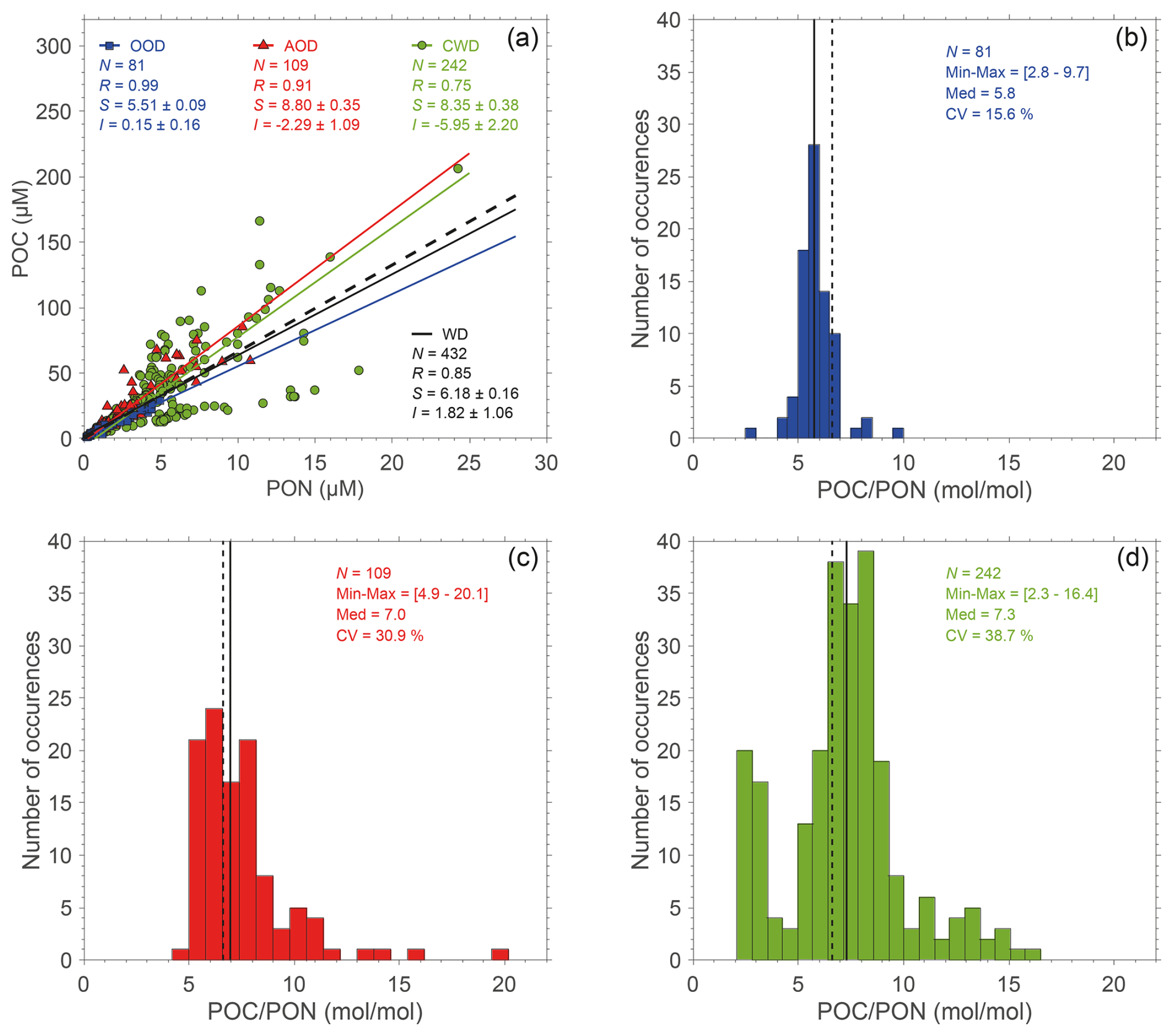
Figure 5 (a) Scatterplot of PON as a function of POC, where the data points are color coded to distinguish between the three data subsets, OOD (blue squares), AOD (red triangles), and CWD (green circles). The solid blue, red, and green lines define the Model-II best-fit linear regression functions calculated for OOD, AOD and CWD, respectively. The solid black line denotes the best-fit function for the whole dataset, WD. The dashed black line shows the Redfield ratio (POC $/$ PON = $\mathrm{106}/\mathrm{16}$ mol mol⁻¹). The number of data points, N; the coefficient of correlation, R; and the slope, S, and intercept, I, of the best-fit linear functions are indicated. The standard deviation of the slope, S, and intercept, I, is indicated. (b) Frequency distribution of the POC $/$ PON ratio (mol mol⁻¹) for the open-ocean dataset, OOD. (c) Same as panel (b) but for the Arctic Ocean dataset, AOD. (d) Same as panel (b) but for the coastal-water dataset, CWD. In panels (b), (c), and (d), the vertical solid black lines correspond to the median values. The vertical dashed black line refers to the Redfield ratio value of 6.625. The values for the minimum-to-maximum range (Min–Max), median (Med), and coefficient of variation (CV) are also provided.

3 Results and discussion

3.1 POC vs. PON relationship

The carbon-to-nitrogen ratio of the organic particulate matter, POC $/$ PON, in our dataset and deviations in these data from the canonical Redfield ratio of $\mathrm{106}/\mathrm{16}$ mol mol⁻¹ (approximately 6.6) are depicted in Fig. 5. We note that in this illustration, we present POC and PON in micromolar concentration units because such units were used in the original work on the Redfield ratio (Redfield, 1934; Redfield et al., 1963). POC and PON are generally well correlated, with R=0.85 for the whole dataset (WD), but the linear regression fitted to the POC vs. PON data deviates slightly from the relationship corresponding to the canonical Redfield ratio (Fig. 5a). For WD, the slope S of the best-fit linear function is 6.18±0.18, which is lower than the Redfield ratio value.

When considering the three subsets of data, the open-ocean data (OOD) exhibit the strongest correlation between POC and PON (R=0.99, Fig. 5a) and the lowest variability in POC $/$ PON (coefficient of variation CV = 15.5 %, Fig. 5b). The median value of POC $/$ PON for open-ocean data is 5.8 (Table 1, Fig. 5b), which is significantly lower than the Redfield ratio. In striking contrast to OOD, the coastal-water dataset (CWD) has the lowest correlation between POC and PON (R=0.75, Fig. 5a) and the highest variability in POC $/$ PON (CV = 38.7 %, Fig. 5d). Moreover, the slope of the best-fit function for CWD ($S=\mathrm{8.35}\pm \mathrm{0.38}$) deviates significantly from the relationship corresponding to the canonical Redfield ratio. It is also notable that the intercept differs significantly from 0 ($I=-\mathrm{5.95}\pm \mathrm{2.20}$, Fig. 5a), which indicates an excess of PON relative to POC. The median of POC $/$ PON for CWD is 7.3 (Table 1, Fig. 5d), which is significantly higher than the Redfield ratio and is the highest among the three data subsets. For the Arctic dataset (AOD), POC and PON are highly correlated (R=0.91, Fig. 5a). The variation in POC $/$ PON is large, with a CV value of 30.9 % (Fig. 5c), which is twice as high as in the open-ocean dataset but somewhat lower than in the coastal-water dataset. The median of POC $/$ PON for AOD is 6.9, which is closer to the Redfield ratio than the median values for OOD and CWD.

The results presented in Fig. 5 are consistent with expectations regarding the variability in POC $/$ PON in aquatic environments and with previous reports on such variability. For example, Geider and La Roche (2002) compiled data on oceanic POC $/$ PON from multiple sources and reported a large range of variation, between 3.4 and 12.5 mol mol⁻¹. It is also known that the variation in inland waters is even larger, with POC $/$ PON reaching values that are much higher than the Redfield ratio (Bauer et al., 2013). The compilation of data from different inland aquatic environments showed a POC $/$ PON range of 7.5–22.6 for lake environments (They et al., 2017) and 6.5–15.7 for rivers (Liu et al., 2020). Many measurements in our coastal-water dataset (CWD) were collected in areas affected by river plumes and associated input of terrestrial particulate organic matter, which explains the large variability, including the presence of high values of POC $/$ PON in this dataset (Fig. 5a, d). The lowest values of this ratio (<4) in CWD correspond to data collected in the northern Adriatic Sea and are consistent with the previously reported values from this environment (Faganeli et al., 1989). The observed general trend of an increase in POC $/$ PON variability from the open-ocean dataset to the coastal-water dataset reflects the increased complexity of the factors that drive the variation in the elemental composition of the bulk particulate organic matter. Different patterns of variability and deviations of measured POC $/$ PON from the canonical Redfield ratio can be attributed to regional variations in environmental conditions, plankton biodiversity (Martiny et al., 2013), and carbon-enriched terrestrial inputs and/or preferential remineralization of PON relative to POC (Dauby et al., 1994; Engel et al., 2002; Ferrari et al., 2003). Overall, the results of the PON $/$ POC variability support the notion that PON cannot be reliably estimated from POC using the assumption of the Redfield ratio.

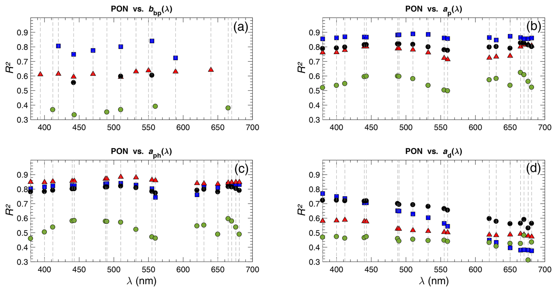
Figure 6 Coefficients of determination (R²) between log₁₀-transformed PON and particulate IOPs as a function of light wavelength. (a) PON vs. b_bp(λ), (b) PON vs. a_p(λ), (c) PON vs. a_ph(λ), and (d) PON vs. a_d(λ). The black circles, blue squares, red triangles, and green circles refer to R² calculated at selected light wavelengths for the whole dataset (WD) and the open-ocean (OOD), Arctic Ocean (AOD), and coastal-water (CWD) datasets, respectively. The data points for R² vs. b_bp(λ) in panel (a) are at the following wavelengths: 394, 412, 420, 442, 470, 490, 510, 532, 550, 555, 560, 589, 640, and 665 nm. The selected wavelengths for the absorption coefficients in panels (b), (c), and (d) are 380, 400, 412, 440, 443, 488, 490, 510, 532, 555, 560, 620, 630, 650, 665, 670, 676, and 689 nm.

3.2 Development of PON vs. IOP relationships

The particulate IOPs, b_bp(λ), a_p(λ), a_ph(λ), and a_d(λ), available in our dataset were measured at multiple light wavelengths as described in Sect. 2.2. For the development of the relationships between PON and IOPs, our primary interest is in examining the IOPs at selected light wavelengths that are consistent with the spectral bands used on several past and current satellite ocean color sensors. Figure 6 depicts the spectral pattern of the coefficient of determination, R², between log₁₀-transformed PON and the four particulate IOPs at selected light wavelengths. In these calculations, the number of selected wavelengths is smaller for b_bp(λ) (Fig. 6a) than for the absorption coefficients (Fig. 6b, c, d), which is associated with the spectral coverage of these measurements in our dataset. In addition, the results in Fig. 6 are shown for the whole dataset (WD) and separately for the three data subsets, OOD, AOD, and CWD. In general, the spectral patterns of R² for most illustrated cases are relatively flat. A few exceptions include the spectral variations in R² for the PON vs. a_d(λ) relationship, especially for the open-ocean dataset (Fig. 6d), as well as some variations associated with the main spectral bands of phytoplankton absorption for the relationships involving a_p(λ) and a_ph(λ) (Fig. 6b, c). The R² values are generally substantially lower for the coastal-water dataset, CWD, compared to OOD and AOD. This result is expected, given that the largest variability in PON and IOPs is in CWD.

In subsequent sections, we present the relationships between PON and IOPs for a few selected wavelengths, specifically PON vs. b_bp(λ) at 555 nm, and PON vs. a_p(λ), a_ph(λ), and a_d(λ) at 442 and 510 nm. At these wavelengths, the R² values in Fig. 6 either are close to the maximum or remain relatively high within the spectral pattern of R². A more complete set of the relationships for other wavelengths that are commonly used on satellite ocean color sensors is provided in the Supplement (Tables S1 to S3).

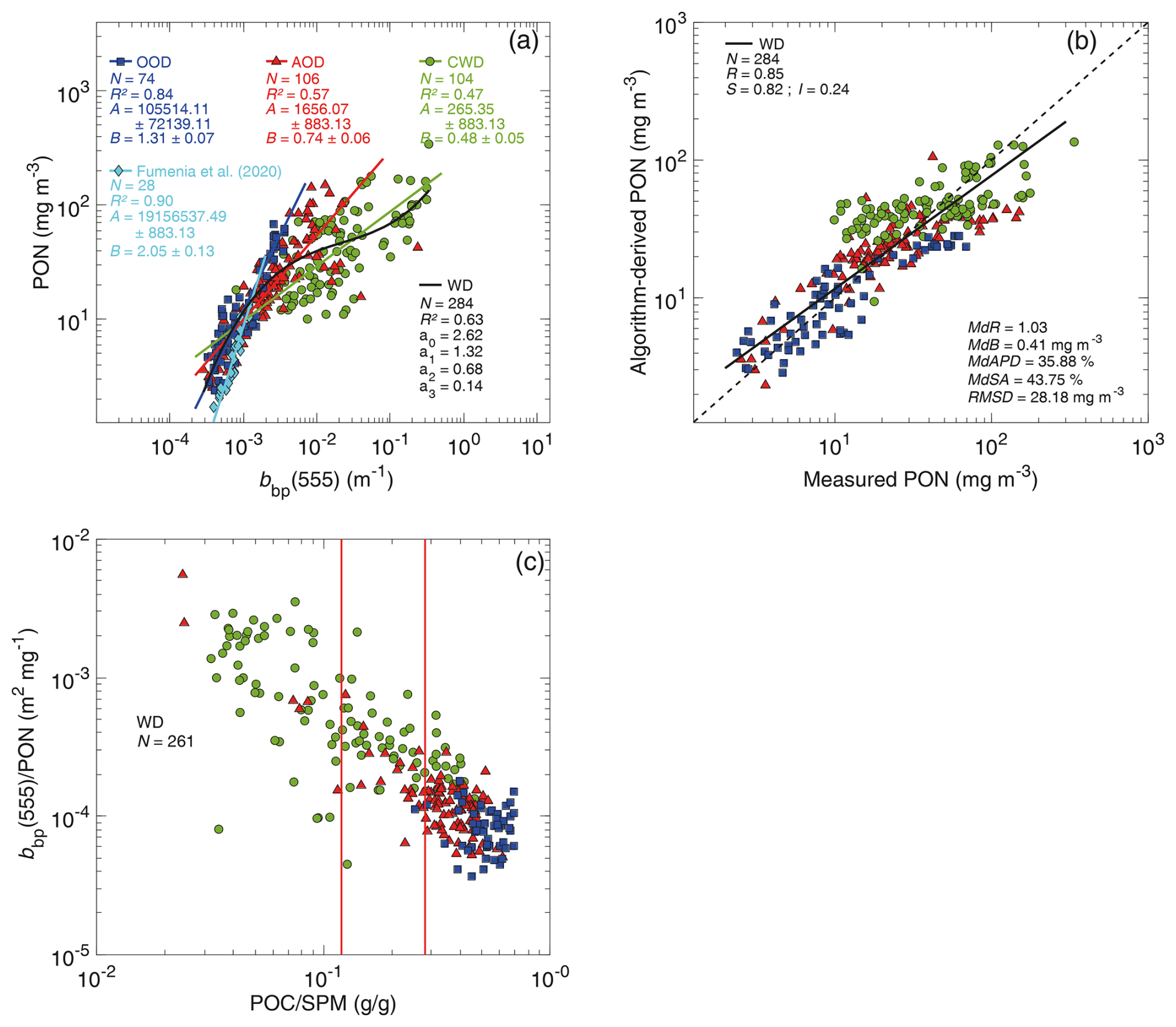
Figure 7 (a) Relationships between PON and b_bp(555) for different datasets, as indicated by dark-blue squares, red triangles, and green circles corresponding to the open-ocean dataset (OOD), Arctic Ocean dataset (AOD), and coastal-water dataset (CWD), respectively. The solid dark-blue, red, and green lines represent the best-fit power functions obtained from the Model-II linear regression on log₁₀-transformed data. The solid black line represents the best-fit third-degree polynomial function for the whole dataset (WD). For comparison, data in light blue from Fumenia et al. (2020) are shown after the conversion of measured b_bp(700) to b_bp(555) using a λ⁻¹ spectral dependency. The standard deviation of the best-fit coefficients, A and B, is indicated. (b) Comparison of algorithm-derived and measured PON, where the algorithm is the black line in panel (a) for the whole dataset, WD. The solid black line is the best-fit function obtained from the Model-II linear regression on log₁₀-transformed data. The dashed line represents the 1:1 line. (c) Scatterplot of b_bp(555) $/$ PON vs. POC $/$ SPM. The vertical red lines refer to the threshold values of POC $/$ SPM of 0.12 and 0.28, which delimit the mineral-dominated from mixed particulate assemblages and the mixed from organic-dominated particulate assemblages, respectively (Stramski et al., 2023). Panels (a) and (b) of the figure include the statistical indicators (see Sect. 2.4 for details).

3.3 Relationship between PON and the backscattering coefficient

Figure 7a depicts the relationship between PON and b_bp(555). When the open-ocean dataset (OOD) is considered, the scatter of data is relatively small (blue squares), and the pattern of data suggests that the relationship can be reasonably well described by a power function (dark-blue line):

$$\begin{array}{}\text{(2)}& \text{PON}=\mathrm{105}\mathrm{514.11}(\pm \mathrm{72}\mathrm{139.11})b_{\mathrm{bp}}(\mathrm{555}{)}^{\mathrm{1.31}(\pm \mathrm{0.07})},\end{array}$$

where the values in parentheses indicate the standard deviation of the best-fit coefficients. For this subset of data, the coefficient of determination between the log₁₀-transformed data is high (R²=0.84). For comparison, Fig. 7a also includes a recently established relationship in the open-ocean waters of the western tropical South Pacific using in situ measurements of b_bp from BGC-Argo floats (Fumenia et al., 2020). While the number of these data is comparatively small and the data cover a relatively narrow range of PON, from about 0.28 to 13.3 mg m⁻³, it is notable that this relationship is consistent with the relationship described by Eq. (2) for our larger open-ocean dataset (OOD).

When the Arctic Ocean (AOD) and coastal-water (CWD) datasets are considered, the scatter of data points is much larger, and the relationships between PON and b_bp(555) are considerably weaker. The R² values for these two datasets drop to 0.57 and 0.47, respectively. As a result, the relationship for the whole dataset (WD) is also relatively weak, with a moderate R² of 0.63. Importantly, the overall pattern of all data in WD no longer suggests that a single power function of PON vs. b_bp(555) can provide a reasonable description of the general trend of data observed across this whole dataset. In this case, the pattern of data suggests that the relationship can be described reasonably well by a third-degree polynomial function (black line):

$$\begin{array}{}\text{(3)}& \mathrm{PON}={\mathrm{10}}^{[\mathrm{2.62}+\mathrm{1.32}{\log }_{\mathrm{10}}\left(b_{\mathrm{bp}}\left(\mathrm{555}\right)\right)+\mathrm{0.68}[{\log }_{\mathrm{10}}\left(b_{\mathrm{bp}}\left(\mathrm{555}\right)\right){]}^{\mathrm{2}}+\mathrm{0.14}\left[{\log }_{\mathrm{10}}\left(b_{\mathrm{bp}}\left(\mathrm{555}\right)\right){]}^{\mathrm{3}}\right]}.\end{array}$$

A comparison of the algorithm-derived and measured values of PON is presented in Fig. 7b. This plot and the associated statistical metrics provide a means to evaluate how the best-fit third-degree polynomial function of PON vs. b_bp(555) for the whole dataset (WD) from Fig. 7a reproduces the PON variability for this algorithm development dataset. Figure 7b shows a deviation between the linear fit to data and the 1:1 line, which indicates that the b_bp(555)-based algorithm overestimates the PON values at low PON and tends to underestimate at high PON. Recognizing these biasing effects in different PON ranges is important, especially as MdR is very close to 1, indicating that an aggregate bias for the whole dataset (WD) is very small. Other statistical indicators displayed in Fig. 7b are related to significant scatter of data points around the 1:1 line; for example, MdAPD is about 35.9 %.

The results in Fig. 7a, b demonstrate that b_bp(555) cannot be used as a good proxy for PON within the wide range of PON and b_bp(555) variability observed across diverse marine bio-optical environments. This conclusion also holds for the backscattering coefficient at other light wavelengths (not shown) and is not surprising because the various physical–chemical characteristics of natural particulate assemblages, which affect the optical properties of particles, are highly variable across diverse environments. Also, this conclusion is consistent with earlier studies that examined the estimation of POC from optical measurements, including the backscattering coefficient, across a wide range of aquatic environments. For example, a recent study of measurements from the western Arctic seas, which exhibit a large range of variability, demonstrated that the generally poor relationships based indiscriminately on all data can be improved by accounting for variations in the composition of particulate matter parameterized in terms of the POC $/$ SPM ratio (Stramski et al., 2023). This is because this ratio can serve as a proxy for the contribution of organic particles to the total suspended particulate matter, which also includes mineral particles. In turn, the proportion of organic and mineral particles is one of the important drivers of variations in particle optical properties, for example through changes in the particle refractive index. Whereas other particle characteristics such as size distribution, shape, or degree of aggregation are also important determinants of particle optical properties, the changes in the compositional parameter of POC $/$ SPM are useful in explaining, at least partly, the variability in the relationships between the measures of particulate organic concentration, such as PON and POC, and the bulk optical properties of seawater. Figure 7c depicts the variations in the PON-specific backscattering coefficient, $b_{\mathrm{bp}}\left(\mathrm{555}\right)/\text{PON}$, as a function of POC $/$ SPM for our whole dataset. The variations span 2 orders of magnitude, with a clear trend of a large decrease in the PON-specific backscattering coefficient together with an increase in POC $/$ SPM (R=0.85), which represents an increase in the proportion of organic particles in the suspended particulate matter. For data corresponding to mineral-dominated particulate assemblages (POC $/$ SPM <0.12), the median value is $b_{\mathrm{bp}}\left(\mathrm{555}\right)/\text{PON}=\mathrm{9.91}\times {\mathrm{10}}^{-\mathrm{4}}$ m² mg⁻¹. The median drops by a factor of about 9 to a value of $\mathrm{1.07}\times {\mathrm{10}}^{-\mathrm{4}}$ m² mg⁻¹ for data encompassing the organic-dominated assemblages (POC $/$ SPM >0.28). To the first order, this trend is attributable to the fact that while organic particles contribute to both PON and b_bp, the mineral particles contribute only to b_bp. Overall, these results support the notion that, similar to the POC-specific particulate backscattering coefficient, the PON-specific particulate backscattering coefficient is also strongly dependent on particulate composition.

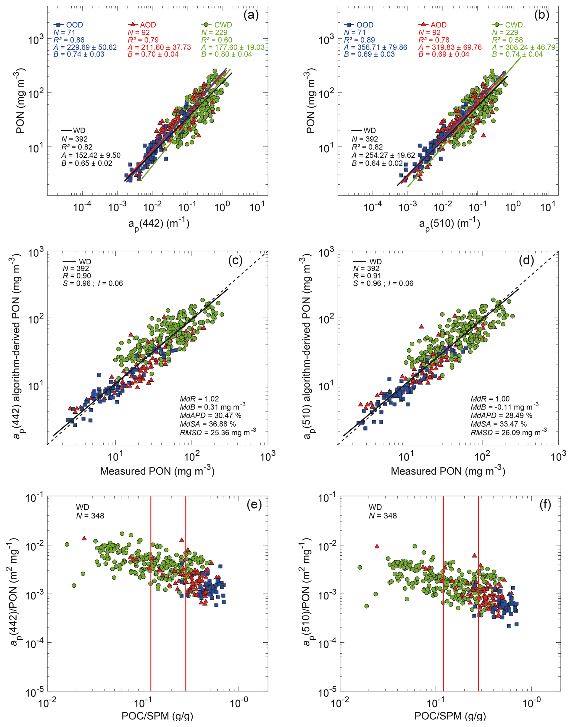
Figure 8 (a) Relationships between PON and a_p(442) for different datasets, as indicated by dark-blue squares, red triangles, and green circles corresponding to the open-ocean dataset (OOD), Arctic Ocean dataset (AOD), and coastal-water dataset (CWD), respectively. The solid dark-blue, red, green, and black lines represent the best-fit power functions obtained from the Model-II linear regression on log₁₀-transformed data for the OOD, AOD, CWD, and the whole dataset (WD), respectively. The standard deviation of the best-fit coefficients, A and B, is indicated. (b) Same as panel (a) but for a_p(510). (c) Comparison of algorithm-derived and measured PON, where the a_p(442)-based algorithm is the black line in panel (a) for the whole dataset, WD. The solid black line is the best-fit function obtained from the Model-II linear regression on log₁₀-transformed data. The dashed line represents the 1:1 line. (d) Same as panel (c) but for the a_p(510)-based algorithm. (e) Scatter plot of a_p(442)/PON vs. POC $/$ SPM. The vertical red lines refer to the threshold values of POC $/$ SPM of 0.12 and 0.28, which delimit the mineral-dominated from mixed particulate assemblages and mixed from organic-dominated particulate assemblages, respectively (Stramski et al., 2023). (f) Same as panel (e) but for $a_{\mathrm{p}}\left(\mathrm{510}\right)/\text{PON}$. Panels (a), (b), (c), and (d) of the figure include the statistical indicators (see Sect. 2.4 for details).

3.4 Relationships between PON and absorption coefficients

We now turn to relationships between PON and absorption coefficients, specifically the total particulate absorption coefficient, a_p(λ), and its phytoplankton, a_ph(λ), and non-algal, a_d(λ), components. Figure 8a, b depict data of PON vs. a_p(λ) for two selected wavelengths of light, 442 and 510 nm. In contrast to results for b_bp(555) (Fig. 7a), the best-fit power functions for PON vs. a_p(λ) are similar for the whole dataset, WD, and for its subsets, OOD, AOD, and CWD, considered separately. This result indicates a relatively weak sensitivity of a_p-based PON algorithms to the natural variability observed across diverse marine bio-optical environments. For WD, the determination coefficient is R²=0.82, which is much higher compared to the 0.63 for the relationship based on b_bp(555). Also, the scatter of all data points around the best-fit functions of PON vs. a_p(442) or a_p(510) is largely reduced compared to the relationship of PON vs. b_bp(555). The best-fit power functions for the whole dataset, WD, are

$$\begin{array}{}\text{(4)}& {\displaystyle }\text{PON}=\mathrm{152.42}(\pm \mathrm{9.50})a_{\mathrm{p}}(\mathrm{442}{)}^{\mathrm{0.65}(\pm \mathrm{0.02})}\text{(5)}& {\displaystyle }\text{PON}=\mathrm{254.27}(\pm \mathrm{19.62})a_{\mathrm{p}}(\mathrm{510}{)}^{\mathrm{0.64}(\pm \mathrm{0.02})}.\end{array}$$

It is also notable that if the data subsets OOD, AOD, and CWD are considered separately, the relationships between PON vs. a_p(λ) are strongest for the open-ocean dataset (R²=0.86 or 0.89) and progressively weaken through the Arctic to the coastal-water dataset (for the latter R²=0.60 or 0.58; Fig. 8a, b).

Figure 8c, d support reasonably good agreement between PON derived from the a_p-based algorithms and PON measured over the whole range of variability observed within WD. The best-fit regression functions of algorithm-derived vs. measured PON do not exhibit large deviations from the 1:1 line. The aggregate bias is negligibly small, with MdR = 1 or 1.02. For all data in WD, a_p(442) and a_p(510) reproduce the PON variability, with MdAPD values slightly below 30.5 %, which is an improvement compared with 35.9 % for the PON estimation from b_bp(555).

Figure 8e, f show that the PON-specific particulate absorption coefficients, $a_{\mathrm{p}}\left(\mathrm{442}\right)/\text{PON}$ and $a_{\mathrm{p}}\left(\mathrm{510}\right)/\text{PON}$, exhibit variations spanning more than 1 order of magnitude with a decreasing trend associated with an increase in POC $/$ SPM (R=0.66 and 0.63 for the two light wavelengths selected, 442 and 510 nm, respectively). The trend is accompanied by about three-fold decrease in the median value of PON-specific a_p(λ); for example, the median of $a_{\mathrm{p}}\left(\mathrm{510}\right)/\text{PON}$ decreases from $\mathrm{5.5}\times {\mathrm{10}}^{-\mathrm{2}}$ to $\mathrm{1.6}\times {\mathrm{10}}^{-\mathrm{2}}$ m² mg⁻¹ as the composition of particulate matter changes from mineral dominated to organic dominated. While the variations in PON-specific a_p(λ) have an impact on the ability to predict PON from a_p(λ), these effects are weaker compared to the case of the particulate backscattering coefficient.

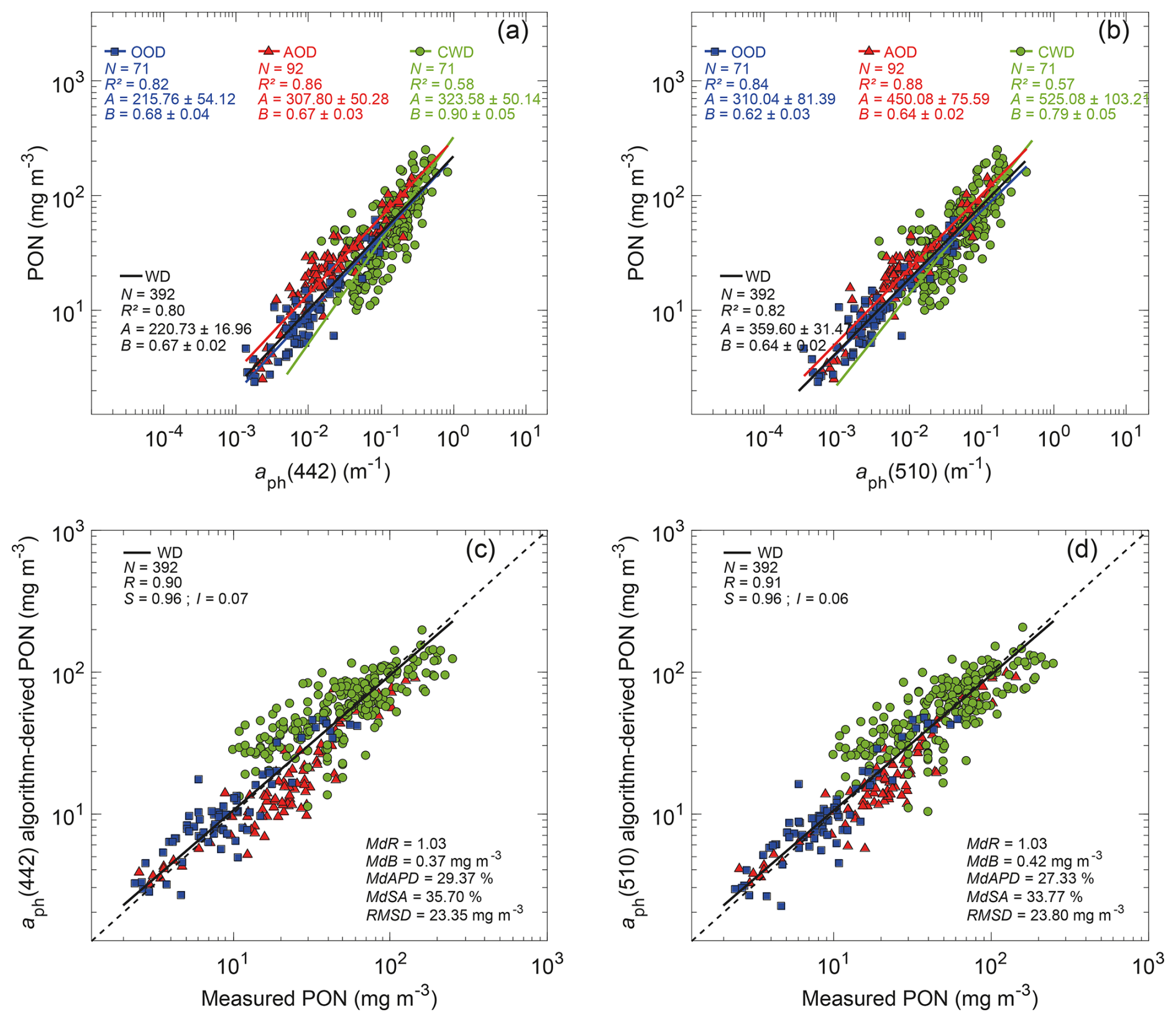
Figure 9 (a) Relationships between PON and a_ph(442) for different datasets, as indicated by dark-blue squares, red triangles, and green circles corresponding to the open-ocean dataset (OOD), Arctic Ocean dataset (AOD), and coastal-water dataset (CWD), respectively. The solid dark-blue, red, green, and black lines represent the best-fit power functions obtained from Model-II linear regression on log₁₀-transformed data for the OOD, AOD, CWD, and the whole dataset (WD), respectively. The standard deviation of the best-fit coefficients, A and B, is indicated. (b) Same as panel (a) but for a_ph(510). (c) Comparison of algorithm-derived and measured PON, where the a_ph(442)-based algorithm is the black line in panel (a) for the whole dataset, WD. The solid black line is the best-fit function obtained from the Model-II linear regression on log₁₀-transformed data. The dashed line represents the 1:1 line. (d) Same as panel (c) but for the a_ph(510)-based algorithm. Each panel of the figure includes the statistical indicators (see Sect. 2.4 for details).

Figure 9 depicts similar results to Fig. 8 but for the phytoplankton absorption coefficients, a_ph(442) and a_ph(510). Although PON is associated with both phytoplankton and non-algal organic particles and the experimental determinations of a_ph(λ) are intended to represent the light absorption by phytoplankton pigments only, Fig. 9 shows that a_ph(λ) has an ability to predict PON that is comparable to the total particulate absorption coefficient a_p(λ). The best-fit functions for the whole dataset, WD, are (Fig. 9a, b)

$$\begin{array}{}\text{(6)}& {\displaystyle }\text{PON}=\mathrm{220.73}(\pm \mathrm{16.96})a_{\mathrm{ph}}(\mathrm{442}{)}^{\mathrm{0.67}(\pm \mathrm{0.02})}\text{(7)}& {\displaystyle }\text{PON}=\mathrm{359.60}(\pm \mathrm{31.47})a_{\mathrm{ph}}(\mathrm{510}{)}^{\mathrm{0.64}(\pm \mathrm{0.02})}.\end{array}$$

For these a_ph-based algorithms, the statistical metrics based on comparisons of algorithm-derived and measured PON (Fig. 9c, d) are very similar to those for the a_p-based algorithms (Fig. 8c, d). For example, the MdR values remain very close to 1, and MdAPD is slightly below 30 %. When separate subsets of data are considered, the relationship between PON and a_ph(λ) is strongest for the open-ocean and Arctic datasets and weaker for the coastal-water dataset. As expected, the PON-specific phytoplankton absorption coefficient is weakly correlated with the proportion of organic particles in the suspended particulate matter (R=0.47 and 0.46 for the two light wavelengths selected, 442 and 510 nm, respectively, figure not shown).

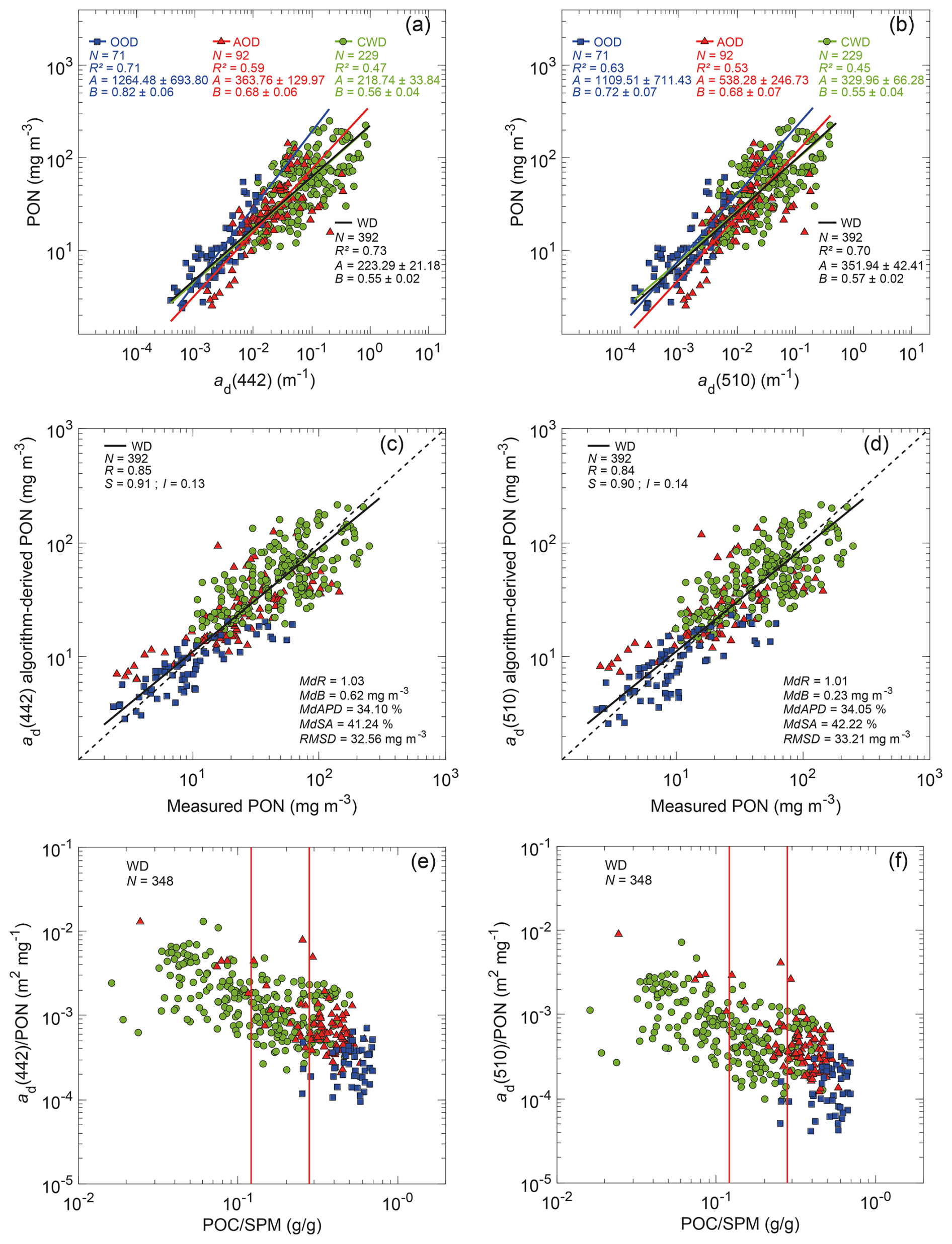
Figure 10 Same as Fig. 8 but for the non-algal particulate absorption coefficients a_d(442) and a_d(510).

In contrast to the a_p-based and a_ph-based PON algorithms, the PON vs. a_d(λ) relationships are not as strong, although they exhibit less inter-dataset variability compared to the b_bp-based relationships (Fig. 10a, b). In particular, the slope of the best-fit functions for the open-ocean dataset (OOD) differs significantly from the best-fit functions for AOD and CWD. The best-fit functions for the whole dataset, WD, are

$$\begin{array}{}\text{(8)}& {\displaystyle }\text{PON}=\mathrm{223.29}(\pm \mathrm{21.18})a_{\mathrm{d}}(\mathrm{442}{)}^{\mathrm{0.55}(\pm \mathrm{0.02})}\text{(9)}& {\displaystyle }\text{PON}=\mathrm{351.94}(\pm \mathrm{42.41})a_{\mathrm{d}}(\mathrm{510}{)}^{\mathrm{0.57}(\pm \mathrm{0.02})}.\end{array}$$

but these a_d-based algorithms are inferior to the a_p-based and a_ph-based algorithms for estimating PON across the wide dynamic range of PON and IOPs observed within the whole dataset. Figure 10c, d show increased uncertainty in PON predicted from Eqs. (7) and (8) for all data included in WD, which is manifested in particular through the increased values of MdB, MdAPD, MdSA, and RMSD. Variations in the particulate composition parameterized by the POC $/$ SPM ratio exert a similar influence on the $a_{\mathrm{d}}\left(\mathit{\lambda }\right)/\text{PON}$ ratio (R=0.67 and 0.61 for the two light wavelengths selected, 442 and 510 nm, respectively, Fig. 10e, f) compared to the case of the $a_{\mathrm{p}}\left(\mathit{\lambda }\right)/\text{PON}$ ratio (Fig. 8e, f).

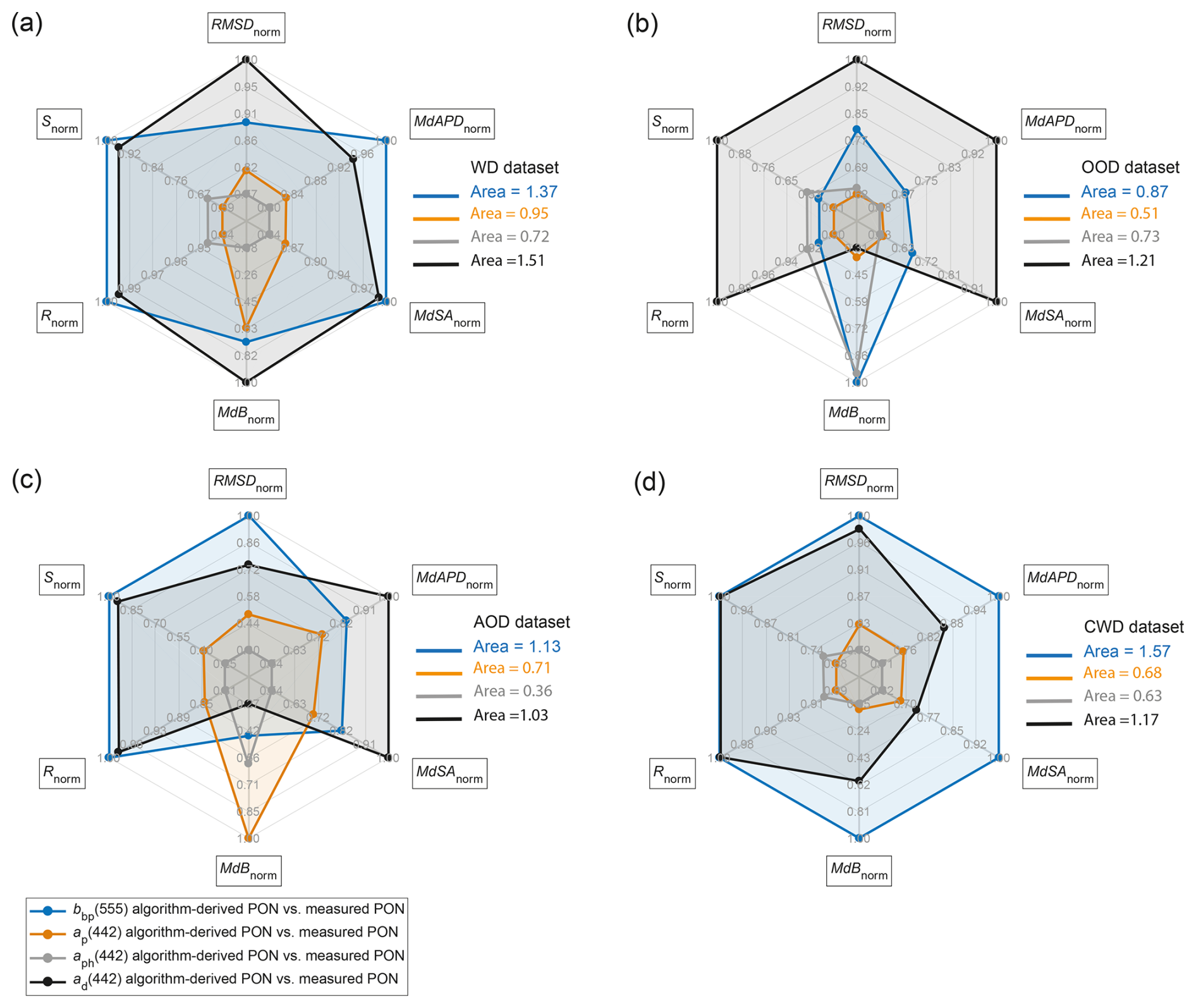
Figure 11 Radar plots summarizing the performance of the IOP-based algorithms for deriving PON. The IOP(λ)s considered are the b_bp(555) (blue line), a_p(442) (orange line), a_ph(442) (gray line), and a_d(442) (black line). The smallest area of the polygon associated with each algorithm represented in the radar plot corresponds to the best performance. The coefficient of correlation, R; slope, S; root-mean-square deviation, RMSD; median bias, MdB; median absolute percentage difference, MdAPD; and median symmetric accuracy, MdSA, subject to appropriate normalization (see Sect. 2.4), are indicated for (a) WD, (b) OOD, (c) AOD, and (d) CWD.

4 Concluding remarks

The analysis of the empirical relationships between PON and particulate IOPs indicate that the total particulate, a_p(λ), and phytoplankton, a_ph(λ), absorption coefficients have the potential to be used as predictive variables in IOP-based algorithms for estimating PON over a wide range of oceanic environments. Specifically, the analysis of near-surface measurements from various open-ocean and coastal regions including Arctic waters shows consistent relationships of PON vs. a_p(λ) or vs. a_ph(λ) across datasets collected in different marine bio-optical environments. For the whole dataset considered in this study to formulate the a_p-based and a_ph-based algorithms in the form of power functions, the median absolute percent difference between the algorithm-derived and measured PON is slightly less than 30 %. The relationships of PON vs. the non-algal particulate absorption coefficient, a_d(λ), or vs. the particulate backscattering coefficient, b_bp(λ), are weaker, especially when a wide dynamic range of PON and IOPs within the whole dataset is considered. However, for the subset of data from open-ocean waters, our results indicate that b_bp(555) can serve as a reasonably good proxy for PON and that this result is consistent with earlier data from a more geographically restricted region of the western tropical Pacific (Fumenia et al., 2020).

To further support these conclusions, a comparative assessment of the goodness-of-fit associated with the different versions of the IOP-based algorithms when evaluated with the whole dataset (WD) as well as its component subsets, the open-ocean dataset (OOD), Arctic Ocean dataset (AOD), and coastal-water dataset (CWD), is presented using radar plots in Fig. 11. The radar plots are particularly effective for a synthetical comparison of the performance of algorithms using multiple statistical metrics simultaneously (e.g., Tran et al., 2019; Bonelli et al., 2021, 2022). Figure 11 illustrates the areas of polygons created by six statistical indicators that include R, S, MdB, MdAPD, MdSA, and RMSD after appropriate normalization (Sect. 2.4). The size of the polygon area is related to the quality of the goodness-of-fit for a given algorithm as evaluated using its development dataset. As the area of the polygon becomes smaller, the overall representation of PON variability by the algorithm improves, and hence the algorithm has greater potential for better performance. Figure 11 supports the conclusion that the a_p-based and a_ph-based algorithms best represent the PON variability over a large dynamic range within the whole dataset, WD, as well as within the separate data subsets, OOD, AOD, and CWD. The b_bp-based algorithm may perform reasonably well only in open-ocean waters. This result can be relevant to efforts aiming at the estimation of PON from optical sensors deployed on in situ autonomous platforms such as BGC-Argo floats.

Given the relative scarcity of concurrent PON and IOP measurements across a wide range of marine bio-optical environments, in the present study all available data were used to examine and formulate the PON vs. IOP relationships, and no independent data were available for validation. In general, the performance of the algorithms is limited by the variability in the relationships between PON and particulate IOPs that, in turn, is associated with multiple factors, such as variations in the composition and size distribution of suspended particulate matter that drive variations in PON-specific IOP coefficients. In this study, we demonstrate these effects by showing the variations in PON-specific IOP coefficients with changes in POC $/$ SPM ratio, providing information about the relative proportions of organic and mineral particles. Accounting for such variability appears desirable if further improvements are to be achieved in the performance of optically based PON algorithms across diverse oceanic environments. This research avenue has been recently described in relation to POC algorithms (Stramski et al., 2023; Koestner et al., 2024). To further support this research, there is a clear need to collect more concurrent measurements of seawater optical properties and various characteristics of suspended particles in diverse aquatic environments, including the measures of particulate concentration such as PON, POC, and SPM, as well as some measures of particle size and composition that also play important roles in bio-optical variability. The availability of more extensive datasets can help with both the development of improved algorithms and validation with independent data.

Given that the seawater constituent IOPs can be estimated from different inverse optical models (e.g., Zheng and Stramski, 2013; Loisel et al., 2018; Jorge et al., 2021; Kehrli et al., 2024), in future work it will be desirable to investigate whether the IOP-based algorithms presented in this study can provide a means for remote-sensing retrievals of PON using IOPs derived from satellite ocean color observations. The potential significance of the estimation of PON from spaceborne remote-sensing platforms is wide-ranging. For example, knowledge of the carbon-to-nitrogen ratio of organic particulate matter, POC $/$ PON, is important to link the carbon and nitrogen cycles (Martiny et al., 2013). While the POC $/$ PON Redfield ratio remains a reasonable approximation for global ocean biogeochemical studies, the POC $/$ PON ratio can exhibit significant regional and temporal variability (Geider and La Roche, 2002; Martiny et al., 2013). Accounting for this variability is critical for advancing our understanding of the role of phytoplankton in biogeochemistry, for calculating export production, and for refining ocean productivity models (Falkowski, 2000; Geider and La Roche, 2002). As the ocean color algorithms for estimating POC have reached a relatively high level of maturity (Stramski et al., 2022; Kong et al., 2024), combining the existing POC algorithms with novel PON algorithms offers a tool to study the variability in the POC $/$ PON ratio over a range of spatial and temporal scales from satellite remote-sensing observations.