Amplified bottom water acidification rates on the Bering Sea shelf from 1970–2022

The Bering Sea shelf supports a highly productive marine ecosystem that is vulnerable to ocean acidification (OA) due to the cold, carbon-rich waters. Previous observational evidence suggests that bottom waters on the shelf are already seasonally undersaturated with respect to aragonite (i.e. Ω_arag<1) and that OA will continue to increase the spatial extent, duration, and intensity of these conditions. Here, we use a regional ocean biogeochemical model to simulate changes in ocean carbon chemistry for the Bering Sea shelf from 1970–2022. Over this timeframe, model results suggest that surface Ω_arag decreases by −0.043 per decade and surface pH by −0.014 per decade, comparable to observed global rates of OA. However, bottom water pH decreases at twice the rate of surface pH, while bottom [H⁺] decreases at nearly 3 times the rate of surface [H⁺]. This amplified bottom water acidification has emerged over the past 25 years and is likely driven by a combination of anthropogenic carbon accumulation and increasing primary productivity and subsurface respiration and remineralization. Due to this enhanced bottom water acidification, the spatial extent of bottom waters with Ω_arag<1 has greatly expanded over the past 2 decades, along with pH conditions harmful to red king crab. Interannual variability in surface and bottom Ω_arag, pH, and [H⁺] has also increased over the past 2 decades, resulting in part from the increased physical climate variability. We also find that the Bering Sea shelf is a net annual carbon sink of 1.1–7.9 Tg C yr⁻¹, with the range resulting from the difference in the two different atmospheric forcing reanalysis products used. Seasonally, the shelf is a significant carbon sink from April–October but a somewhat weaker carbon source from November–March.

1 Introduction

The global ocean presently absorbs 25 %–31 % of annual CO₂ emissions, making it a critical carbon sink that mitigates anthropogenic warming (Gruber et al., 2019; Friedlingstein et al., 2020; McKinley et al., 2020). The uptake of this anthropogenic carbon has driven a shift in the marine carbonate system towards a state of lower pH and carbonate saturation, a process referred to as ocean acidification (OA; Feely et al., 2004). High-latitude regions are particularly vulnerable to OA due to the poorly buffered, cold temperature waters generating naturally low-carbonate-saturation states (Fabry et al., 2009). Experimental studies have determined a number of negative effects to marine organisms due to OA (Doney et al., 2020), particularly for organisms that form calcium carbonate shells, as these shells become harder to build and maintain as carbonate saturation states (Ω) approach and drop below one. Pteropod shell dissolution has already been observed in several high-latitude environments (Bednarsek et al., 2012; Niemi et al., 2021), and OA is expected to shift these conditions equatorward over time.

Although OA is driven by the increase in atmospheric CO₂ and subsequent increase in ocean carbon uptake, there are a number of physical and biogeochemical processes that can modify the rate of OA expected from the increase in atmospheric CO₂ (Hauri et al., 2021). For example, the accumulation of respired carbon at depth reduces the buffer capacity of subsurface water, leading to amplified subsurface acidification rates compared to surface waters throughout large regions of the global oceans (Fassbender et al., 2023). Coastal shelf systems can experience local rates of acidification much faster than the global oceans due to upwelling (Feely et al., 2008), biological respiration (Feely et al., 2010), eutrophication (Laurent et al., 2017), and changes in circulation (Siedlecki et al., 2021). In the Arctic, changes in sea ice formation (Zhang et al., 2020) and biological productivity and remineralization (Qi et al., 2022) can generate acidification rates 2–3 times greater than the rate for the open oceans.

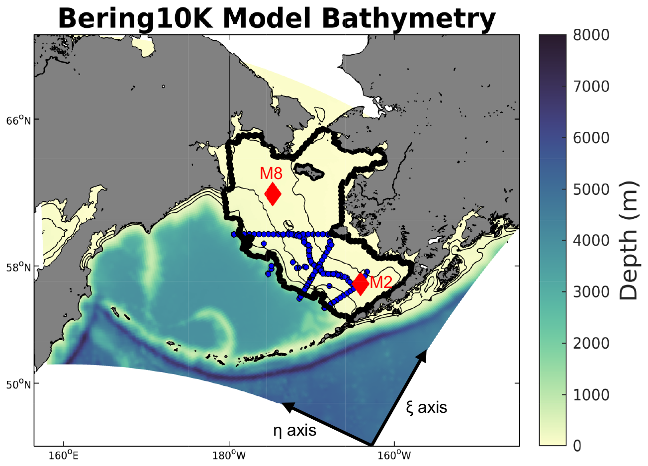
Figure 1 Spatial map of the model domain along with the model bathymetry. Also shown are the discrete ship-based sample locations (blue dots) and the two moorings (red diamonds) used for model validation. The thick black line denotes the spatial region used to encompass the Bering Sea shelf. Also noted at the bottom are the η and ξ axes for the western and southern open boundary conditions, respectively.

The Bering Sea is composed of a relatively large (>500 km wide and >100 km long), shallow eastern coastal shelf along with a narrow western shelf and a deep interior basin. The shelf itself is composed of three distinct biophysical domains (inner, middle, and outer) often delineated by the 50, 100, and 200 m isobaths (Fig. 1). General circulation on the shelf tends to follow these isobaths in a north-northwest direction, eventually feeding into the western intensified Anadyr Current, which then flows through Bering Strait, thereby providing a key conduit between the Bering Sea and Arctic (Kinder et al., 1986; Stabeno et al., 2016). The Bering Sea shelf ecosystem is strongly tied to the atmospheric and oceanic physical forcing, with the seasonal formation and retreat of sea ice playing a fundamental role through the development of the bottom water cold pool and by setting the timing and magnitude of the spring phytoplankton bloom (Brown and Arrigo 2013; Sigler et al., 2014). While the formation of sea ice occurs annually, the areal extent and timing of ice formation and retreat can vary substantially. This variability during the past 10–20 years has consisted of multi-year periods of persistent warm, low sea ice extent (e.g., 2001–2005 and 2014–2018) or cold, high sea ice extent conditions (e.g., 2007–2013; Stabeno et al., 2012). The recent warm years have generated record-breaking low sea ice extent and high temperatures in the northern Bering Sea, with substantial negative impacts to the marine ecosystem (Stabeno and Bell, 2019; Siddon et al., 2020).

On annual timescales, the Bering Sea shelf is generally considered a net carbon sink, driven by substantial spring–summer primary productivity generating low surface ocean pCO₂ values and a net influx of carbon from the atmosphere (Bates et al., 2011; Cross et al., 2014; Pilcher et al., 2019). A portion of the carbon fixed by this mixed-layer productivity sinks to bottom waters where it is respired into inorganic carbon and can be re-emitted back to the atmosphere in fall–winter due to strong atmospheric wind speeds and vertical mixing (Cross et al., 2014; Pilcher et al., 2019). Sea ice further impacts the seasonal carbon cycle by acting as a physical barrier inhibiting air–sea gas exchange. Furthermore, sea ice formation can pump dissolved inorganic carbon (DIC) and total alkalinity to the bottom along with salinity via brine rejection, while sea ice melt dilutes both variables in surface waters (Mortenson et al., 2020).

Previous observational and modeling studies have found that seasonal periods of undersaturation of aragonite (Ω_arag<1) are already occurring within subsurface waters and near regions of significant riverine freshwater runoff (Mathis et al., 2011; Cross et al., 2013; Pilcher et al., 2019). Subsurface Ω_arag<1 waters occur in summer and early fall, driven by bacterial respiration associated with remineralization of sinking organic matter, particularly in regions of high primary productivity in the middle- and outer-shelf domains (Mathis et al., 2011). Surface waters generally maintain much higher values of Ω_arag and pH due to this significant primary productivity, except near freshwater runoff, particularly the mouths of the Yukon and Kuskokwim rivers, where Ω_arag<1 and relatively low pH values are driven by relatively high DIC : TA ratios due to terrestrial carbon exports (Mathis et al., 2011; Pilcher et al., 2019). Furthermore, model simulations suggest that winter surface Ω_arag values are relatively low and close to 1, particularly in ice-covered regions where entrained subsurface carbon cannot re-equilibrate with the atmosphere (Pilcher et al., 2019). Winter observational data are extremely sparse due to challenging weather and sea ice conditions; however, limited late-fall data suggest supersaturated pCO₂ conditions (Cross et al., 2014; Cross et al., 2016). Model simulations project that seasonal periods of surface Ω_arag undersaturation may grow to encompass up to 5 months of the year following the RCP 8.5 emissions scenario and 2–3 months following the RCP 4.5 scenario (Pilcher et al., 2022).

The Bering Sea sustains a substantial US fishery, representing 40 % of US total fish catch by weight and USD 3 billion in annual value (Wiese et al., 2012). These fisheries also provide commercial, subsistence, and cultural benefits to many Alaskan communities, putting them at risk from ocean acidification (Mathis et al., 2015). In the Bering Sea, red and tanner crab have emerged as species particularly vulnerable to the direct effects of OA. The growth rates and survival of larval and juvenile crab for both species are decreased at pH values lower than 7.8 (Long et al., 2013a, b, 2016). Incorporating these results into bioeconomic models suggests that the red king crab fishery could substantially decline if OA is not accounted for in the fisheries management process (Seung et al., 2015; Punt et al., 2016). Recent closures of the snow crab fishery and the Bristol Bay red king crab fishery have had devastating impacts on the Bering Sea commercial fishing community and have led to some discussion concerning the potential role of OA (Siddon, 2022). However, recent laboratory studies have found that snow crab appear resilient to OA (Algayer et al., 2023) and that the snow crab fishery collapse may be due to a mass mortality event resulting from the 2018–2019 heat wave (Szuwalski et al., 2023). In comparison to the collapse in snow crab populations, the Bristol Bay red king crab fishery has been in a steady decline since 2014 (Fedewa et al., 2020). Although model results suggest that bottom waters in parts of Bristol Bay have pH values harmful to larval and juvenile red king crab, these crab populations tend to inhabit nearshore regions that are relatively well buffered with much higher pH values (Pilcher et al., 2022). Nonetheless, recent work suggests that OA may be contributing to recruitment failure in the Bristol Bay red king crab fishery (Litzow et al., 2025).

Recent work utilized a regional ocean biogeochemical model and a dynamical downscaling technique to generate long-term projections of OA for the Bering Sea shelf using multiple Earth system models (ESMs) and emissions scenarios (Pilcher et al., 2022). Here, we greatly expand the temporal coverage of our previous model hindcast, which covered 2002–2012 (Pilcher et al., 2019), to now simulate 53 years (1970–2022) of the Bering Sea marine carbon cycle. We use this model output to quantify spatial-temporal trends in Bering Sea shelf marine carbonate variables over the entire hindcast and the underlying mechanisms generating heterogeneity in these trends. We conclude by illustrating how this model output is being incorporated into the fisheries management process and the next steps to continue refining these model-based OA products.

2 Methods

2.1 Base model description

The regional Bering10K model is an implementation of the Regional Ocean Modeling System (ROMS; Shchepetkin and McWilliams, 2005; Haidvogel et al., 2008), with 10 km horizontal resolution and 30 vertical layers. The Bering10K model simulates sea ice formation and melt, along with tidal mixing. A thorough description of the physical model can be found in Hermann et al. (2016) and Kearney et al. (2020). This physical model is coupled to a lower-trophic NPZD model, originally developed as part of the Bering Sea Ecosystem Study (BESTNPZ; Gibson and Spitz 2011) and recently updated by Kearney et al. (2020). Briefly, the BESTNPZ model simulates two phytoplankton groups (small and large), five zooplankton groups (microzooplankton, small copepods, large copepods, euphausiids, and jellyfish), three nutrient groups (nitrate, ammonium, iron), and two detrital groups (slow and fast sinking). BESTNPZ also contains an ice biology sub-model which simulates ice algae, nitrate, and ammonium, along with a benthic sub-model which simulates a benthic infauna group and a detrital group. A thorough description of the BESTNPZ model can be found in Kearney et al. (2020).

Carbonate chemistry is incorporated into the Bering10K BESTNPZ model by simulating DIC and total alkalinity (TA), which are used to calculate the remainder of the carbonate system following the OCMIP-2 protocols and CO2SYS (Lewis and Wallace, 1998). Here we report pH and [H⁺] values on the total scale. DIC is generated from planktonic respiration and detrital remineralization and consumed via planktonic photosynthesis. Additionally, DIC is exchanged with the atmosphere depending on the gradient in the partial pressure of CO₂ between the surface ocean and the atmosphere (DpCO₂) and the wind speed following Wanninkhof (2014). The atmospheric CO₂ concentration is set to the monthly in situ concentration from the NOAA Barrow Observatory in Alaska (Thoning et al., 2022). This time series started in 1973; for 1970–1972, we take the 1973 Barrow monthly time series and subtract the respective annual growth rate from the Mauna Loa time series (https://gml.noaa.gov/ccgg/trends/, last access: November 2024). Riverine freshwater runoff flux is prescribed following freshwater discharge data from 28 watersheds in Alaska and Russia, including the Yukon River, which supplies roughly 50 % of the total freshwater flux to the Bering Sea shelf (Kearney, 2019). This river runoff contains seasonally varying concentrations of DIC (1480–4100 µmol kg⁻¹) and TA (1238–2743 µmol kg⁻¹) following data collected at Pilot Station at the mouth of the Yukon River (Striegl et al., 2007; PARTNERS, 2010; Pilcher et al., 2019).

The atmospheric forcings for air temperature, sea level pressure, longwave and shortwave radiation, u and v winds, specific humidity, and rainfall are provided by a combination of reanalysis products. For 1970–1994 we use the Common Ocean Reference Experiment (CORE; Large and Yeager, 2009) forcing, for 1995–2011 the Climate Forecast System Reanalysis (CFSR; Saha et al., 2010), and for 2011–2021 the Climate Forecast System Operational Analysis (CFSv2-OA; Saha et al., 2014). Lateral open boundary conditions at weekly resolution for temperature, salinity, and oceanic velocities (u and v) are derived from the larger-scale Northeast Pacific model (NEP5), which has nominal 10 km horizontal resolution and 60 vertical layers (Danielson et al., 2011) for the CORE forcing timeframe. The CFSR forcing timeframe uses the CFSR/CFSv2-OA ocean values at a zonal resolution of $\mathrm{1}/\mathrm{2}$° and a variable meridional resolution of $\mathrm{1}/\mathrm{4}$° between 10° N and 10° S, increasing to $\mathrm{1}/\mathrm{2}$° poleward of 30° N and 30° S, and a total of 40 vertical layers (Saha et al., 2010). Nitrate boundary conditions are monthly climatologies from a long-term run of the larger Northeast Pacific (NEP5) ROMS domain (Danielson et al., 2011). Oxygen initial conditions and monthly boundary conditions are climatologic means from the World Ocean Atlas 2018 product (Garcia et al., 2018). Water column iron concentrations are nudged towards empirical climatological profiles, which use an analytical function based on Seward line data in the Gulf of Alaska for coastal regions (Hinckley et al., 2009). On-shelf values are set at 2.0 mmol m⁻³ at the surface and 4.0 mmol m⁻³ at depth, and this gradient transitions linearly to 0.01 mmol m⁻³ at the surface and 2.0 mmol m⁻³ at depth in water depths greater than 100 m.

The lateral boundary conditions for DIC and TA are calculated via linear regressions with salinity through the following equations, derived from observational data collected primarily from 2008–2010 (Pilcher et al., 2019).

$$\begin{array}{}\text{(1)}& {\displaystyle }S<\mathrm{32.6}& {\displaystyle }\mathrm{\text{DIC}}=\mathrm{58.5}\cdot S+\mathrm{191.2}+\mathrm{\Delta }\text{DIC}(t{)}^{\mathrm{atmo}}\text{(2)}& {\displaystyle }S\ge \mathrm{32.6}& {\displaystyle }\mathrm{\text{DIC}}=\mathrm{140.4}\cdot S-\mathrm{2478.7}+\mathrm{\Delta }\text{DIC}(t{)}^{\mathrm{atmo}}\text{(3)}& {\displaystyle }S<\mathrm{33.6}& {\displaystyle }\mathrm{\text{TA}}=\mathrm{49.6}\cdot S+\mathrm{600.6}\text{(4)}& {\displaystyle }S\ge \mathrm{33.6}& {\displaystyle }\mathrm{\text{TA}}=\mathrm{141.8}\cdot S-\mathrm{2494.4}\end{array}$$

The salinity–DIC regression has changed over time as the oceanic uptake of CO₂ has increased the DIC concentration of waters, with no effect on salinity. Thus, using this same relationship for the boundary conditions at the start of the hindcast in 1970 would artificially increase DIC. To account for changes in DIC over time, we center the DIC–salinity relationship on the year 2009 (i.e., midpoint of 2008–2010 sampling timeframe) and subtract (add) DIC for years before (after) 2009. The DIC value added or subtracted (ΔDIC^atmo in Eqs. 1–2) for year (t) is obtained from the linear trend in DIC (Fig. S1) calculated from the historical runs of the Coupled Model Intercomparison Phase 6 (CMIP6) over the 1970–2009 timeframe from the mean of three different Earth system models (GFDL-ESM4, CESM2, and MIROC-ES2L). These three ESMs were selected as they have been used previously in the Bering10K regional dynamical downscaling (Cheng et al., 2021; Pilcher et al., 2022). We chose to use this method to gain the higher spatial resolution, particularly in the vertical, provided by the ESM output. We only use the DIC trend from the CMIP6 ESMs and omit any TA trend because the TA trends over this timeframe are much smaller and are tied to changes in salinity (Hinrichs et al., 2023), which is accounted for in our salinity–TA relationship at the boundary.

Initial conditions for the start of the hindcast in 1970 for non-carbonate chemistry variables are taken from a 30-year model spin-up using repeating 2001 forcing (Kearney et al., 2020). Initial conditions for TA are calculated using the same salinity regression used for the boundary conditions. Similarly, the DIC initial conditions use the salinity regression, along with subtracting the same long-term trend used for the boundary conditions. The model is then spun-up for an additional 3 years using repeating 1970 forcing, at which point the model seasonal CO₂ cycle was approximately in balance with minimal year-to-year on-shelf variations. The model hindcast is then started and run continuously for 1970–2022.

2.2 Model updates

A new addition to the BESTNPZ model presented in previous work is the inclusion of oxygen cycling following Siedlecki et al. (2015) and Bianucci et al. (2011). Oxygen cycling contains phytoplankton growth as a source and respiration, remineralization, and nitrification as sinks. Oxygen cycling throughout the water column is governed by the following equation:

$$\begin{array}{}\text{(5)}& \begin{array}{rl}{\displaystyle \frac{\partial {\mathrm{O}}_{\mathrm{2}}}{\partial t}}& ={\text{Phy}}_i\cdot u_i\left(\text{Light},N\right)-\text{resp}\left({\text{Phy}}_i\right)-\text{resp}\left(Z_i\right)\\ & -\text{remin}\left(D_i\right)-\text{nitrification}+\text{advection}+\text{diffusion}.\end{array}\end{array}$$

Surface and bottom oxygen concentrations are further modified through the following equations, respectively:

$$\begin{array}{}\text{(6)}& {\displaystyle }{\left.{\displaystyle \frac{\partial {\mathrm{O}}_{\mathrm{2}}}{\partial t}}\right|}_{\mathrm{surface}}={\displaystyle \frac{V_{{\mathrm{O}}_{\mathrm{2}}}}{\mathrm{\Delta }z}}\cdot \left({\left[{\mathrm{O}}_{\mathrm{2}}\right]}_{\mathrm{sat}}-{\left.\left[{\mathrm{O}}_{\mathrm{2}}\right]\right|}_{z=\mathrm{surface}},\right.\text{(7)}& {\displaystyle }{V}_{{\mathrm{O}}_{\mathrm{2}}}=\mathrm{0.251}{u}^{\mathrm{2}}{\left({\displaystyle \frac{\mathit{Sc}}{\mathrm{660}}}\right)}^{-\mathrm{0.5}},\text{(8)}& {\displaystyle }\begin{array}{rl}{\left.{\displaystyle \frac{\partial {\mathrm{O}}_{\mathrm{2}}}{\partial t}}\right|}_{\mathrm{bottom}}& ={\displaystyle \frac{\mathrm{1}}{\mathrm{\Delta }z}}\left(W_{\mathrm{D}}{\left.{\displaystyle \frac{\mathrm{d}D}{\mathrm{d}z}}\right|}_{z=\mathrm{bottom}}\right)-\text{resp}\left(\text{Ben}\right)\\ & -\text{excretion}\left(\text{Ben}\right)-\text{remin}\left(\text{DetBen}\right),\end{array}\end{array}$$

where Phy_i is the phytoplankton group; u_i is the growth rate; “Light” and N are the light and nutrient limitations, respectively; “resp” is respiration; Z_i is the zooplankton group; “remin” is bacterial remineralization; and D_i is the detrital group. For the surface Eq. (6), Δz is the vertical thickness of the grid cell, [O₂]_sat is calculated following the equation from Garcia and Gordon (1992), Sc is the Schmidt number, and $V_{{\mathrm{O}}_{\mathrm{2}}}$ is the gas transfer velocity following Wanninkhof (2014). For the bottom Eq. (8), W_D is the detrital sinking rate, “Ben” is the benthic infauna group, and “DetBen” is benthic detritus. The above model Eqs. (5)–(8) utilize constant stoichiometric molar ratios consisting of $\mathrm{C}:\mathrm{N}=\mathrm{106}:\mathrm{16}$ and ${\mathrm{O}}_{\mathrm{2}}:\mathrm{N}=\mathrm{138}:\mathrm{16}$ for nitrate fluxes and ${\mathrm{O}}_{\mathrm{2}}:\mathrm{N}=\mathrm{106}:\mathrm{16}$ for ammonium fluxes. The complete BESTNPZ model equations are found in Kearney et al. (2020).

2.3 Observational data for model validation

To assess overall model skill, we compare model hindcast output to several observational datasets. One of the largest available datasets for carbonate chemistry in the Bering Sea was collected and compiled during the 2008–2010 Bering Sea Ecosystem Study (BEST) and Bering Sea Integrated Research Program (BSIERP). This dataset is particularly valuable due to the large number of discrete DIC and TA samples; these are the prognostic model variables used within the model and therefore provide a direct model–data comparison. These data were typically collected in the spring (April and May) and summer (June and July) seasons, along with a fall (September and October) sample period in 2009. The sampling regime covered a large portion of the US southeastern Bering Sea shelf, including three cross-shelf transects (Fig. 1). pCO₂, pH, and Ω_arag values were calculated from DIC, TA, salinity, and temperature measurements using CO2SYS (Cross et al., 2012, 2013).

The M2 mooring is the longest dataset for surface ocean pCO₂ in the Bering Sea. While the M2 mooring itself provides a multi-decadal-long time series of standard oceanographic properties, the moored autonomous surface vehicle (MAPCO2; Sutton et al., 2019) system used to measure pCO₂ was first deployed in 2013 and has since been re-deployed with the M2 mooring during the ice-free season for every year except 2020. Generally, this time series covers the months of May–September; however in 2021 it was left out much later than usual, providing the first glimpse of late-fall and early-winter pCO₂. For further model validation of pCO₂, we also utilize pCO₂ measurements from an Autonomous Surface Vehicle CO₂ (ASVCO2) system onboard the Saildrone uncrewed surface vehicle (USV) (Wang et al., 2022). This dataset provides a transect of surface ocean pCO₂, generally running from the Aleutian Islands to the Bering Strait during missions to the Chukchi Sea from 2017–2019. Therefore, each year contains a northward transect in late spring/early summer, along with a southward transect in late summer.

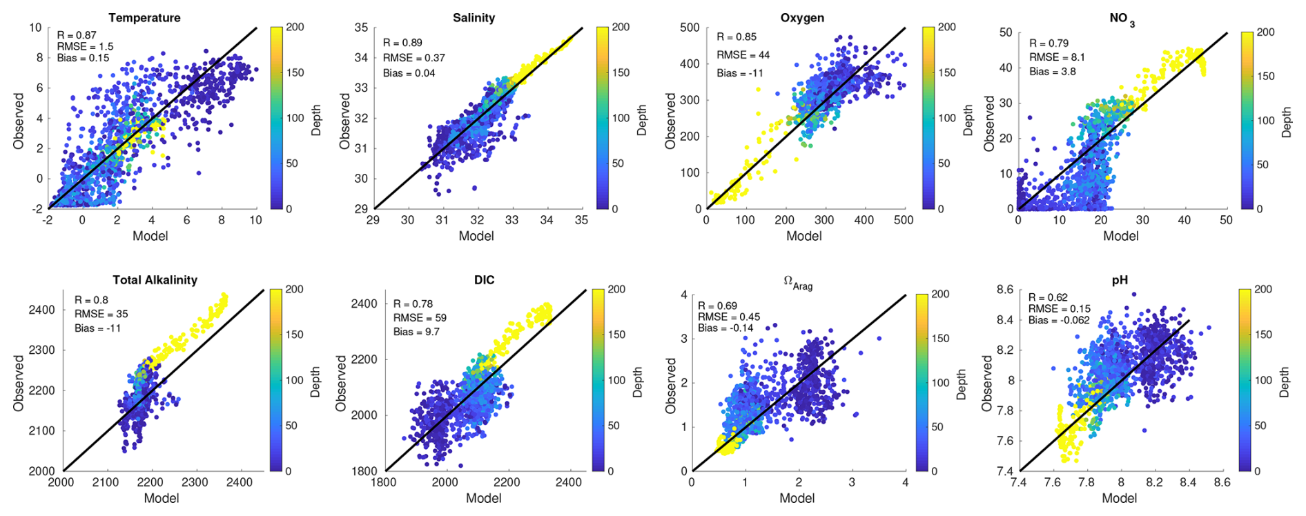
Figure 2 Plots of model (x axis) and observed (y axis) co-located points for different model variables. Also shown in each plot are the R, RMSE, and bias skill statistics. Observed data are from the 2008–2010 BEST–BSIERP project, shown as blue dots in Fig. 1. Note that here the colorbar is constrained to depths between 0–200 m because our focus is on the shelf, though deeper, off-shelf points (denoted by bright yellow dots) are still included.

3 Results

3.1 Model skill assessment

Model property–property comparisons and associated skill statistics between discrete samples collected during 2008–2010 and the model hindcast illustrate relatively high correlation coefficients across the water column for most model prognostic variables (Fig. 2). However, a slight negative TA bias combined with a slight positive DIC bias work synergistically to generate a relatively larger negative bias in Ω_arag and pH. Another notable model–data mismatch is that subsurface points (depth >200 m) for salinity, NO₃, TA, and DIC are all relatively lower in the model compared to the observations. These points are all outside of our definition of the Bering Sea shelf (encompassing depth 0–200 m; Fig. 1) and are located on the shelf break, which is smoothed in the model bathymetry to ensure numerical stability (Kearney et al., 2020). Modeled transport across the shelf break is relatively small, with most on-shelf water arriving through the Aleutian Islands, with shelf water residence times generally less than 3 years (Mordy et al., 2021).

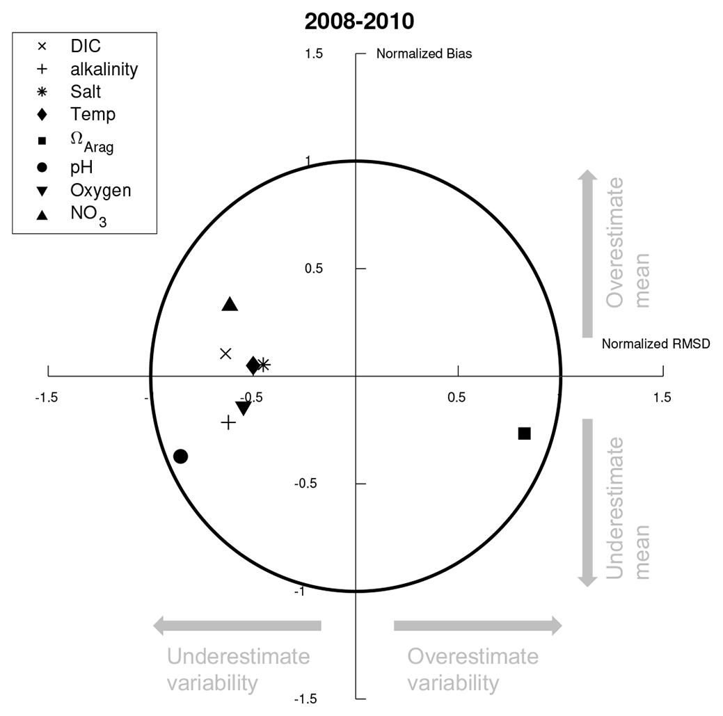
Figure 3 Target diagram summarizing the data comparison from Fig. 2. Here, the x axis is the normalized unbiased RMSD between the model and data, multiplied by the sign of the difference between model and observed standard deviation. The y axis is the normalized mean bias.

The model–data comparison illustrated in Fig. 2 is further summarized via a target diagram (Jolliff et al., 2009) in Fig. 3. In a target diagram, the position in the y axis denotes either a positive (Y>0) or negative (Y<0) normalized model bias, while the position in the x axis signifies whether the model has a larger (X>0) or smaller (X<0) root-mean-square deviation (RMSD) compared to the observed data. The radial distance from the origin (normalized RMSD) is then related to the modeling efficiency metric (MEF; Stow et al., 2009), where model variables that lie within the RMSD <1 circle have an MEF >0, signifying that the model outperforms an estimate based solely on the mean of the observations. Figure 3 illustrates that all highlighted model variables fall within the RMSD value of 1, with relatively low overall biases. Most model variables display less variability compared to the observations, except for Ω_arag which displays more variability.

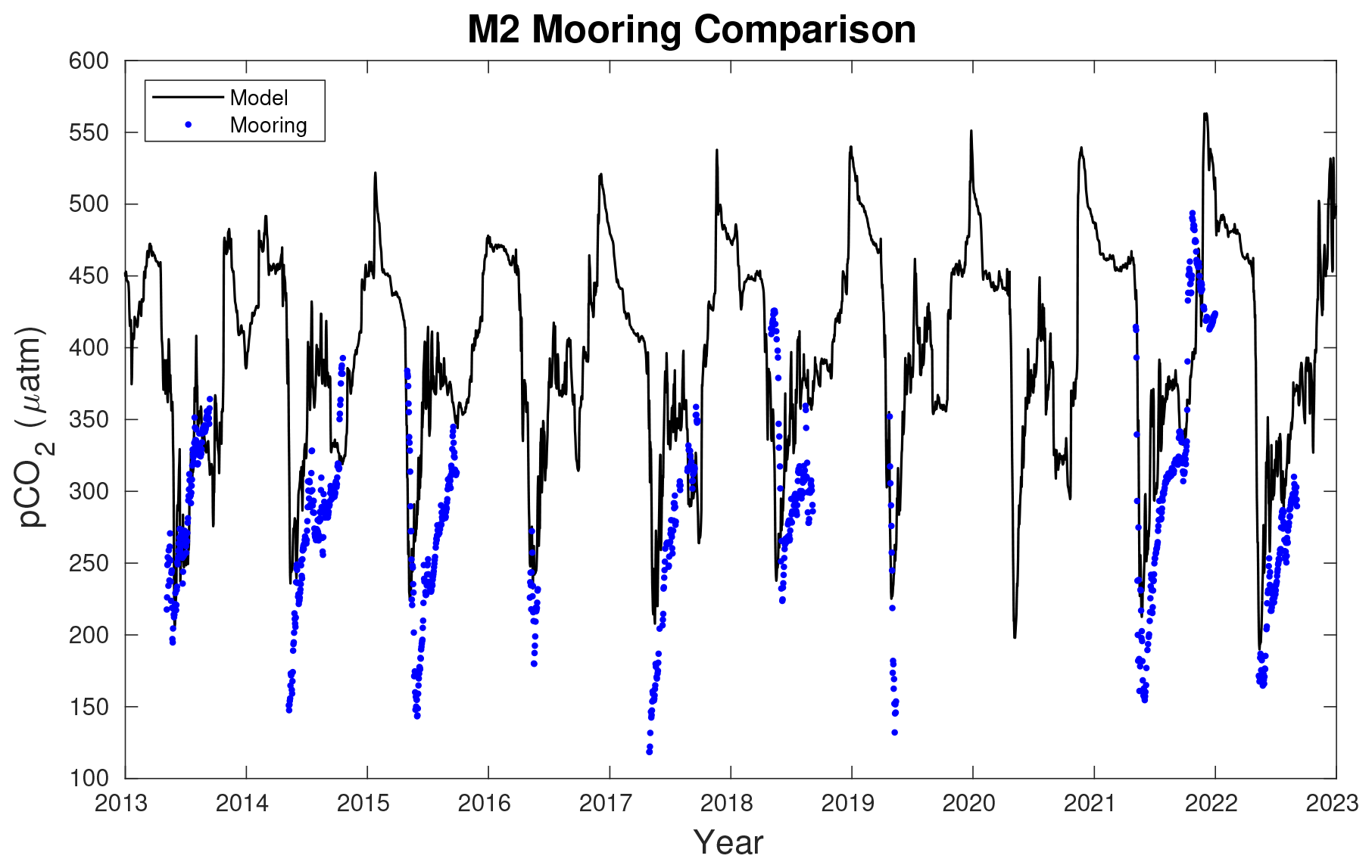
Figure 4 M2 mooring pCO₂ data (blue dots) compared to model daily pCO₂ values (black line) at the equivalent model grid cell location. The mooring is generally deployed in spring and retrieved in fall, though it was out much later in 2021.

In addition to the ship-based observational comparison, model output of surface ocean pCO₂ is also compared to the M2 mooring time series (Fig. 4). The model accurately captures the timing of the late-spring pCO₂ drawdown along with the subsequent increase in pCO₂ leading into summer. Furthermore, the modeled late-fall and early-winter increase in pCO₂ is also apparent in the mooring for the single year that the mooring was left out late into the season. However, the model generally tends to underestimate the magnitude of the late-spring pCO₂ drawdown, which then subsequently leads to model overestimations of summer pCO₂. Notable exceptions are apparent in 2013, 2018, and 2022 when the observed late-spring pCO₂ drawdown was relatively weaker, and the modeled drawdown is more comparable with observations.

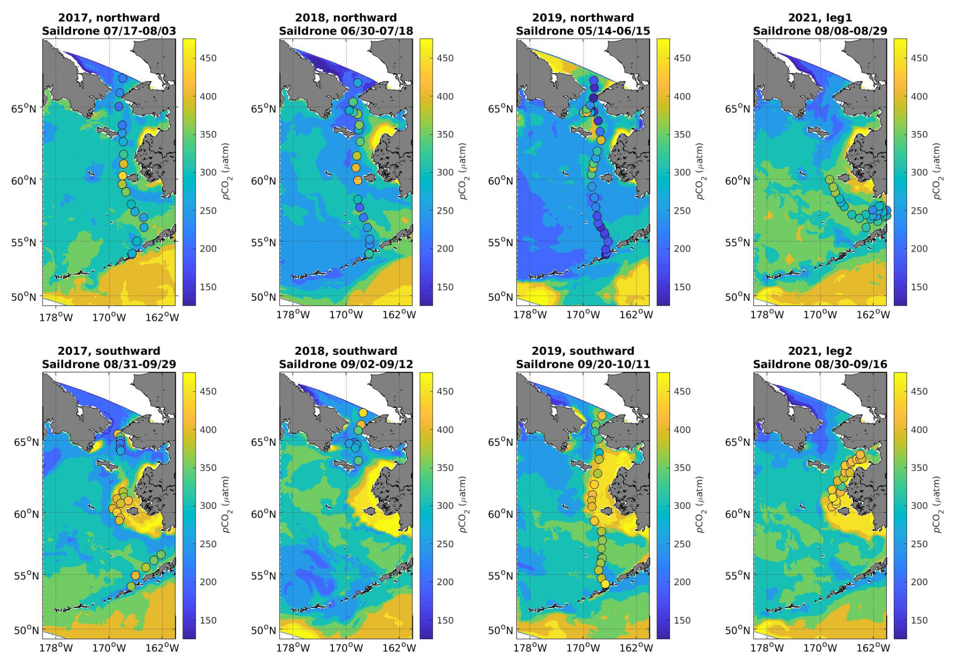
Figure 5 Surface pCO₂ values from Saildrone transects (dots) with model surface pCO₂ values averaged over the equivalent timeframe as the background shading.

Further surface pCO₂ comparisons between the model output and in situ pCO₂ from the autonomous Saildrone platform are shown in Fig. 5. Overall, the model does a reasonably sufficient job of capturing the dominant spatial pattern in pCO₂ illustrated by the Saildrone data, namely the relatively lower pCO₂ values in the southeastern and northern Bering Sea with higher values in the central inner-shelf domain near Nunivak Island. The seasonality between the two transects also aligns, with relatively lower values during the northward transect and higher values during the southward transect. However, the model appears to consistently underestimate the pCO₂ drawdown (i.e., model pCO₂ biased high compared to Saildrone data) in the southeastern Bering Sea during the northward transect, similar to the underestimated spring pCO₂ drawdown from the M2 mooring comparison (Fig. 4). However, the southward transects suggest that this bias is reversed later in the year, when the model is now biased low compared to the Saildrone data, which is also the opposite bias to what we see during the late summer and early fall in the M2 mooring comparison. Additionally, the model tends to underestimate pCO₂ in the central inner-shelf domain just to the west of Nunivak Island. It appears that the Saildrone data are consistently capturing a relatively high plume of pCO₂ in this region. The model also generally simulates these relatively high pCO₂ waters in that region of the inner-shelf domain, but there is a lot of interannual variability and seasonality in this feature.

This analysis suggests that the model is simulating the Bering Sea carbon cycle reasonably well, though there are some noted differences. Namely, the model appears to underestimate variability overall (Fig. 3) and underestimate the magnitude of the seasonal pCO₂ drawdown according to both the M2 mooring and Saildrone data. This could be due to a somewhat smaller-magnitude spring bloom, which is consistent with slight positive model biases in DIC and NO₃ from the ship-based observation comparison (Fig. 2). This bias could translate to model pH and Ω_arag values that are biased low in surface waters but biased high in bottom waters due to less respiration of sinking organic carbon from a smaller spring bloom. However, we caution that bottom measurements are very limited overall and were all collected during the anomalously cold-water conditions during 2008–2010. Furthermore, pCO₂ is a relatively difficult variable for the model to capture because it is a nonlinear, diagnostic variable that is dependent on temperature, salinity, DIC, and TA. This nonlinearity and the potential for synergistic biases (e.g., positive DIC bias but negative TA bias) can generate very large magnitude deviations. Thus, additional bottom water data, particularly for DIC and TA, would be extremely useful in further validating the bottom water carbonate chemistry beyond the 2008–2010 analysis here.

3.2 Impact of forcing on linear trends

The Bering10K BESTNPZ model has historically been utilized for a variety of fisheries management applications (Gibson and Spitz, 2011; Kearney et al., 2020). For these applications, the model hindcast timeframe needed to run through the present and extend back in time to cover major transitions in the Bering Sea during the 1970s and 1980s. At the time, no individual forcing product provided this full timeframe; therefore, it was necessary to combine the CORE and CFSR forcing. Furthermore, the transition between products in 1995 was selected as the 1990s experienced relatively more stable climate variability for the Bering Sea, as this was after the shifts in the 1970s and 1980s but prior to the temperature stanzas of the early 2000s (Stabeno et al., 2012). However, any significant differences in either the atmospheric forcing or the oceanic boundary conditions between the datasets could generate a significant deviation in model results, particularly immediately following the transition in 1995. Furthermore, this transition (i.e., essentially a spin-up to the new model forcing) could generate erroneous linear trends when calculated over the entire timeframe that would represent a shift in the variable over a discrete period rather than a multi-decadal trend. To help clarify this potential influence, we ran a separate simulation which branched off from the primary hindcast simulation in 1995 by continuing the CORE forcing until 2003. We then compared these results to the primary hindcast simulation (e.g., simulation that switches to CFSR in 1995) to assess the effect of this transition in forcing.

Surface and bottom salinity for the Bering Sea shelf provides an example of how the shift in forcing can generate an erroneous long-term trend. A noticeable decrease in salinity of ∼0.5 psu immediately follows the switch to CFSR forcing and oceanic boundary conditions, which does not occur when the CORE forcing and Northeast Pacific model-derived oceanic boundary conditions are extended to 2003 (Fig. S2). This decrease generates a negative trend in surface salinity when calculated over the entire timeframe; however, trends over the individual forcing timeframes are extremely weak and of the opposite sign for the CORE timeframe. This shift in salinity will also impact DIC and total alkalinity through the salinity regression equations used to calculate the horizontal open boundary conditions (Eqs. 1–4). This leads to a decrease in DIC and total alkalinity within the open boundary conditions that is greater in magnitude in intermediate waters (Fig. S3). The effect is greater on DIC relative to TA due to differences in the regression equations. The net effect on shelf-wide conditions is readily apparent for total alkalinity (Fig. S4) but is more muted with DIC, likely due to the relatively stronger effect of biology and air–sea gas exchange.

To account for the potential influence of this transition in forcing, we report all time series linear trends over three timeframes: (1) the complete 1970–2022 CORE-CFSR timeframe, (2) the 1970–1994 CORE timeframe, and (3) the 1998–2022 CFSR timeframe. We start the CFSR trends in 1998 rather than 1995 to account for several years for the transition in forcing, based in part on the re-equilibration to the new forcing by 1998 demonstrated in salinity (Fig. S2). Furthermore, dividing the hindcast into the two timeframes of 1970–1994 and 1998–2022 produces two, equivalent 25-year time slices and will help elucidate any acceleration in trends. Lastly, we show the results of the CORE simulation extended to 2003 for trend estimates in the Supplement, noting which variables exhibit consistent trends throughout both forcing datasets and which variables' long-term trends (estimated over 1970–2022) are impacted by the forcing switch in 1995. The goal with this comparison is not to suggest that trends between the CORE- and CFSR-forced products are the same, but rather our goal is to elucidate which long-term trends result directly from the switch in forcing and which long-term trends emerge within an individual forcing product.

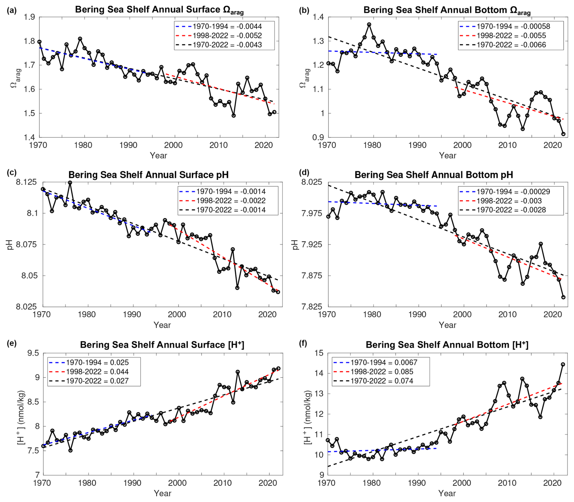
Figure 6 Time series plots of model annual average surface (a, c, e) and bottom (b, d, f) Ω_arag (a, b), pH (c, d), and [H⁺] (e, f) averaged over the Bering Sea shelf region. Also shown are the linear trend values over three different timeframes.

3.3 Bering Sea shelf acidification

Over the 1970–2022 model hindcast, annual surface and bottom Ω_arag and pH decrease, while [H⁺] increases for the Bering Sea shelf, with linear trends greater at the bottom compared to the surface (Fig. 6). We show [H⁺] in addition to pH because pH changes reflect relative [H⁺] changes and are, therefore, not ideal for comparisons between waters with different initial chemistry conditions, such as between surface and bottom waters (Fassbender et al., 2017, 2021). Surface Ω_arag ranges from 1.7–1.8 at the start of the simulation and decreases to 1.5–1.6 by the end, surface pH ranges from 8.1–8.125 and decreases to 8.025–8.05, and surface [H⁺] ranges from 7.5–7.75 nmol kg⁻¹ at the start and increases to 9.25 nmol kg⁻¹ by 2022. Furthermore, the bottom pH trend from 1970–2022 is twice as great as the surface trend, while the bottom [H⁺] trend over the same timeframe is nearly 3 times as great as the surface [H⁺] trend. In fact, bottom acidity, as denoted by [H⁺], increases by approximately 40 % from 1970–2022. These amplified bottom water carbonate trends are strongest over the 1998–2022 timeframe, particularly compared to the relatively weak bottom water trends over the 1970–1994 timeframe. This suggests that the strong bottom water trends evolve over the 1998–2022 timeframe and may be specific to the CFSR forcing. However, the bottom pH trend with CORE forcing increases from −0.0029 per decade when calculated from 1970–1994 to −0.011 per decade when calculated from 1970–2003 (Fig. S5). Thus, the enhanced bottom water trends over the recent timeframe may be sensitive to the forcing product and the specific timeframe over which the trend is calculated. Surface trends in all three carbonate variables are similar across all timeframes, with slightly higher trends from 1998–2022 for pH and [H⁺]. Notably, annual bottom Ω_arag<1 conditions first emerge in 2008 and after 2020 stay below 1 for the remainder of the model simulation. Furthermore, bottom pH values are approaching 7.8 (e.g., conditions demonstrated to negatively affect growth and survival of red king crab; Long et al., 2013a, b) by the end of the model simulation.

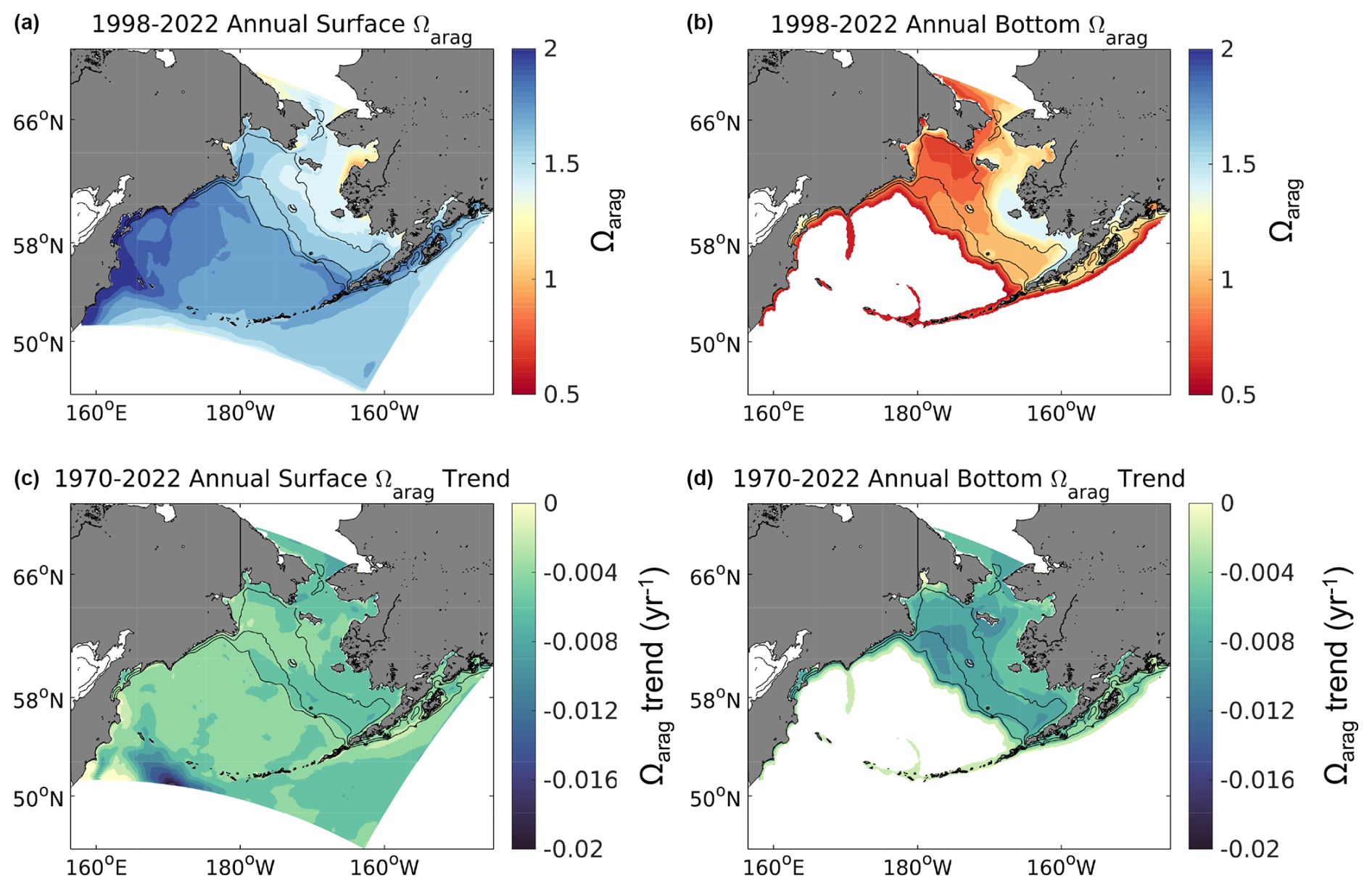
Figure 7 Spatial plots of model annual average surface (a, c) and bottom (b, d) Ω_arag from 1998–2022 (a, b) along with the linear trend for each grid cell (c, d) over the same timeframe. Bottom waters with depths >1500 m are omitted here as our focus is on the shelf.

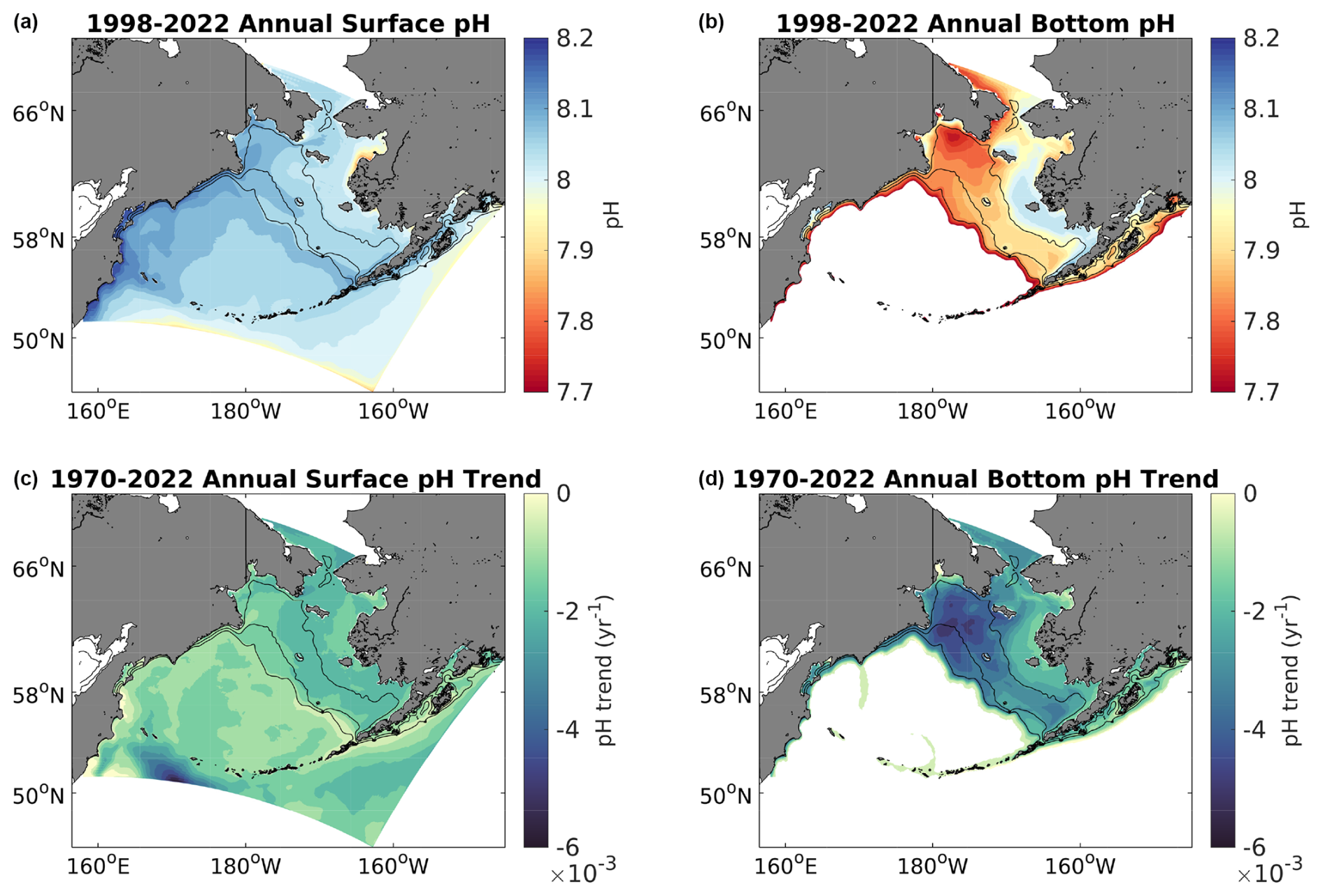
Figure 8 Spatial plots of model annual average surface (a, c) and bottom (b, d) pH from 1998–2022 (a, b) along with the linear trend for each grid cell (c, d) over the same timeframe. Bottom waters with depths >1500 m are omitted here as our focus is on the shelf.

Annual average surface Ω_arag and pH values from 1998–2022 are generally greater on the middle- and outer-shelf domains compared to the inner-shelf domain (Figs. 7–8). Conversely, bottom water values for both variables are generally greater for the inner-shelf domain compared to the middle- and outer-shelf domains. The lowest bottom values tend to occur in the northwest Bering Sea shelf, in the Gulf of Anadyr. Relatively lower values of surface Ω_arag and pH are also apparent near the Yukon River delta. Most shelf surface waters have annual Ω_arag>1.25 and pH ≥8.0. Bottom waters, however, are near or below the aragonite saturation horizon (i.e., Ω_arag=1) for most of the middle and outer shelf, along with pH values <8.0 and near 7.8 for the northwestern middle-shelf domain. Surface Ω_arag and pH trends are spatially fairly consistent throughout the shelf, with slightly stronger, negative trends over the middle shelf and in the northwestern shelf near the Gulf of Anadyr (Figs. 7–8). Bottom water trends for both variables are more spatially heterogenous, with substantially greater trends on the outer-shelf domain compared to the rest of the shelf. This region, along with parts of the southeastern middle-shelf domain, displays stronger, negative trends at the bottom compared to the surface, similar to the shelf-wide averaged time series plots in Fig. 6. [H⁺] trends display similar spatial patterns as pH and are not shown here.

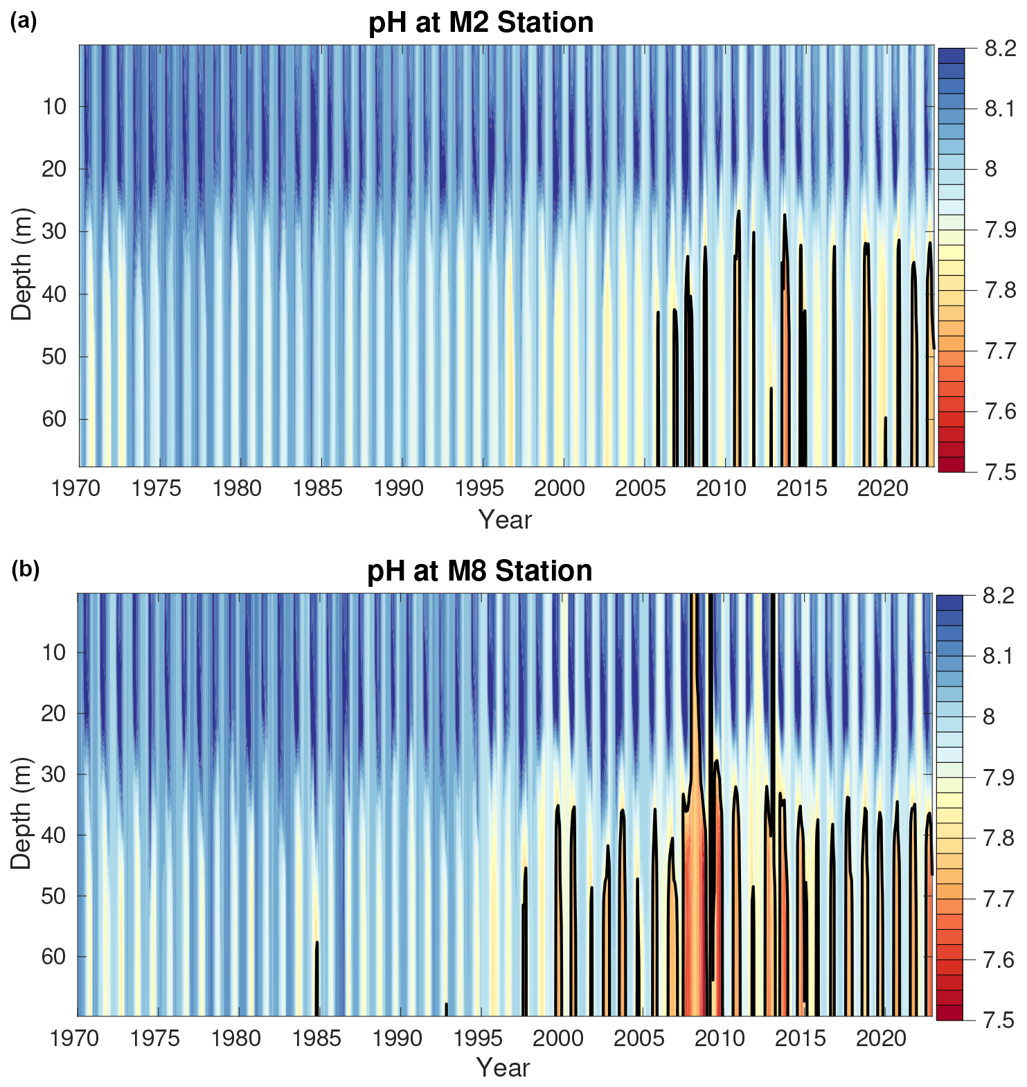
Figure 9 Model monthly averaged pH over the entire model time series at the M2 (a) and M8 (b) approximate model locations. The black contour line denotes the threshold for pH values <7.8, which are conditions harmful to red king crab.

Vertical profiles of modeled pH at the M2 and M8 mooring locations highlight the onset of pH values <7.8 (Fig. 9). At M2, these conditions do not occur in the hindcast until after 2005, at which point they seasonally occur somewhat regularly and shoal to depths between 30–50 m. At M8, pH <7.8 waters rarely occur prior to 2000, after which they occur seasonally every year. In most years, these conditions also shoal to 30–50 m; however, there are several years when they occur throughout the entire water column.

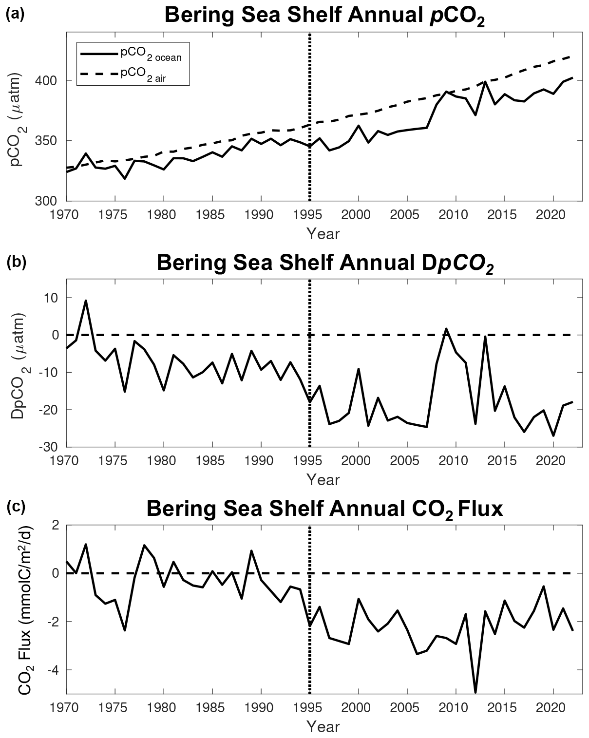
Figure 10 Time series of model annual average (a) surface ocean pCO₂ (black line) and atmospheric CO₂ concentration (dashed line), (b) DpCO₂, and (c) CO₂ flux. Here, DpCO₂ is defined as pCO${}_{\mathrm{2}}^{\mathrm{ocean}}-p$CO${}_{\mathrm{2}}^{\mathrm{atmo}}$ and a negative CO₂ flux signifies a flux of carbon into the ocean. The dotted line denotes the year when the forcing transitions from CORE to CFSR.

3.4 Bering Sea shelf carbon cycle

Atmospheric CO₂ concentrations significantly increase from 328 µatm in 1970 to 420 µatm by 2022, while the surface ocean pCO₂ for the Bering Sea shelf increases from 324 µatm in 1970 to 402 µatm in 2022 (Fig. 10a). This lag in the growth rate of surface ocean pCO₂ compared to the atmosphere generates a net decrease in DpCO₂ (i.e., pCO${}_{\mathrm{2}}^{\mathrm{ocean}}-p$CO${}_{\mathrm{2}}^{\mathrm{atmo}}$) and drives a more negative air–sea CO₂ flux, where a negative flux indicates a flux of carbon into the ocean (Fig. 10b, c). However, the more negative DpCO₂ values with greater carbon fluxes into the ocean tend to occur from 1995–2022, following the switch from CORE to CFSR forcing. Indeed, analysis of the CORE-extended hindcast indicates that the switch in forcing plays a significant role, with the CORE forcing suggesting higher oceanic surface pCO₂ values and more positive CO₂ flux values during the overlapping years (Fig. S6). Furthermore, while there is a negative trend in CO₂ flux over the entire 1970–2022 timeframe (under combined forcing), there is a very minimal negative trend over the 1970–2003 CORE-forced timeframe and a slight positive trend over the 1998–2022 CFSR-forced timeframe, indicating that the transition in forcing is biasing the 1970–2022 trend (Fig. S6). To further illustrate this difference, we calculate the total carbon shelf sink using the spatial area of the shelf (i.e., area defined in Fig. 1; 804 393 km²). For the CORE-forced 1970–1994 timeframe, the shelf was an annual carbon sink of 1.1 Tg C yr⁻¹, compared to an annual carbon sink of 7.9 Tg C yr⁻¹ for the 1998–2022 CFSR-forced timeframe.

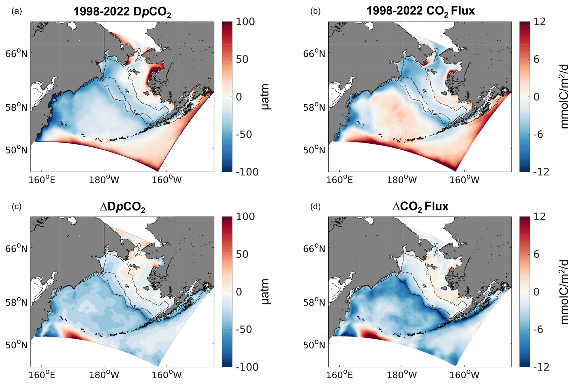
Figure 11 Spatial plots of model annual average surface (a) DpCO₂ and (b) CO₂ flux from 1998–2022. Also shown is (c) ΔDpCO₂ and the (d) ΔCO₂ flux calculated as the difference between the 1998–2022 and the 1970–1994 timeframes.

Figure 11 illustrates that a substantial amount of this annual carbon uptake occurs within the middle- and outer-shelf domains and the northern Bering Sea inner-shelf domain. Conversely, coastal waters near regions of significant riverine runoff (e.g., Yukon and Kuskokwim rivers) are an annual net carbon source. The spatial patterns of air–sea CO₂ flux are largely consistent with the spatial pattern in DpCO₂, though there are some areas where the two variables are not aligned (i.e., not the same sign). This is especially apparent for the off-shelf Bering Sea Basin, which displays slightly negative DpCO₂ values but a relatively strong, positive (i.e., flux out of the ocean) CO₂ flux. The difference of both variables between the CFSR and CORE forcing timeframes illustrates the substantial changes noted in Fig. 10. The off-shelf Bering Sea Basin in particular displays substantially greater-magnitude, negative DpCO₂ and CO₂ flux values during the CFSR-forced timeframe. CO₂ flux values on the outer-shelf domain and near the shelf break are also substantially more negative (i.e., greater carbon uptake) during the CFSR-forced timeframe due to more negative DpCO₂ values.

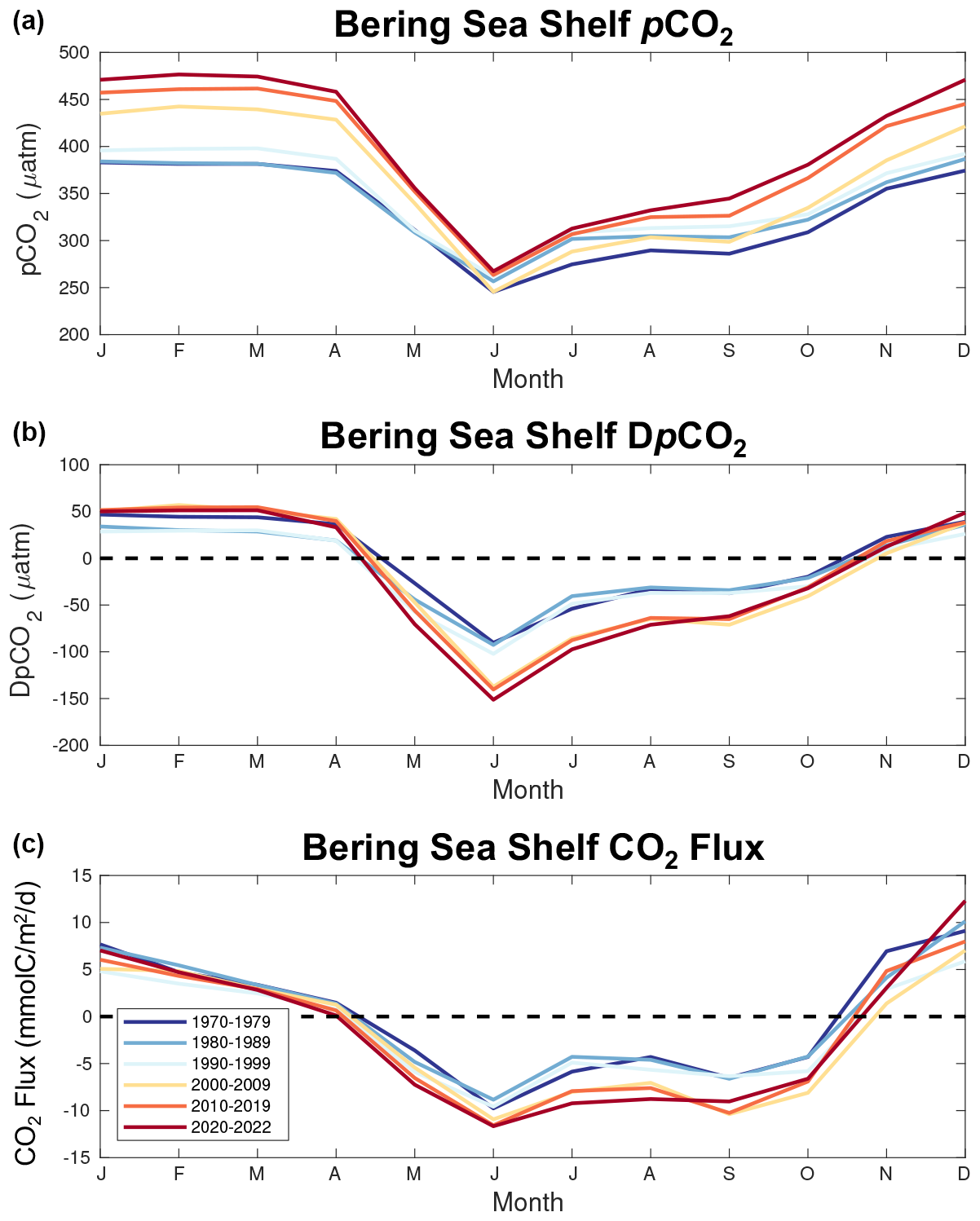
Figure 12 Seasonal plots of model surface ocean pCO₂ (a), DpCO₂ (b), and CO₂ flux (c) averaged over multiple timeframes.

To further investigate the processes leading to the enhanced ocean carbon uptake, we examine the progression of the seasonal carbon cycle over each model decadal timeframe (Fig. 12). These figures reveal a non-uniform seasonal increase in surface ocean pCO₂, with the summer (May–September) values increasing at a much lower rate compared to the rest of the year. For example, the seasonal pCO₂ summer minimum increases by only 22 µatm over the model timeframe, whereas the seasonal winter maximum in January increases by 93 µatm. Atmospheric pCO₂ also increases over this timeframe but with minimal changes in seasonality (i.e., the seasonal amplitude increases by ∼6 µatm over the entire timeframe). The overall effect is a slight reduction in positive CO₂ flux (i.e., less carbon efflux to the atmosphere) during the months when the shelf is a net source of carbon (November–March) but generates greater-magnitude, negative DpCO₂ and CO₂ flux values during the months when the shelf is a net carbon sink (April–September). Notably, these enhanced negative DpCO₂ and CO₂ flux values occur following the transition to CFSR forcing.

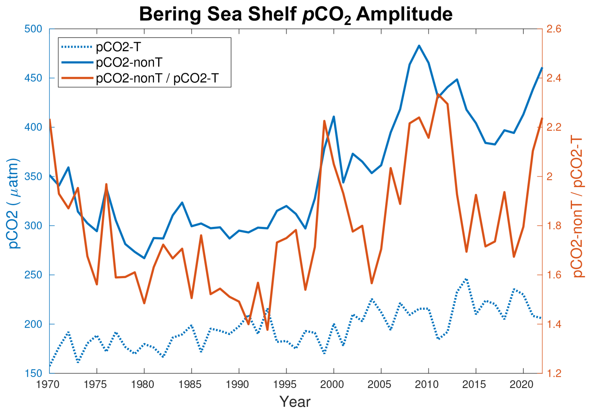
Figure 13 Time series of the yearly maximum seasonal amplitude of pCO₂–T (dotted blue line), pCO₂–nonT (solid blue line), and the ratio of pCO₂–nonT $/$ pCO₂–T (orange line).

To further understand changes in pCO₂, we separate the pCO₂ signal into a temperature component and non-temperature component following Takahashi et al. (2002):

$$\begin{array}{}\text{(9)}& {\displaystyle }p{\mathrm{CO}}_{\mathrm{2}\mathrm{T}}=\stackrel{\mathrm{‾}}{p{\mathrm{CO}}_{\mathrm{2}}}\cdot \exp \left[\mathrm{0.0423}\left(T-\overline{T}\right)\right],\text{(10)}& {\displaystyle }p{\mathrm{CO}}_{\mathrm{2}\mathrm{nonT}}=p{\mathrm{CO}}_{\mathrm{2}}\cdot \exp \left[\mathrm{0.0423}\left(\overline{T}-T\right)\right],\end{array}$$

where the overbars represent the model annual mean values, pCO_2 T is the temperature component reflecting the effect of thermal solubility on pCO₂, and pCO_2 nonT is the remaining pCO₂ effects governed by non-thermal components including biological activity. Following Eqs. (9) and (10), we can calculate the seasonal amplitude of both pCO_2 T and pCO_2 nonT, which gives an indication of which component has a greater effect on determining the seasonal pCO₂. Figure 13 illustrates this comparison throughout the model timeframe. The seasonal amplitudes for both pCO_2 T and pCO_2 nonT increase over the model simulation; however, the amplitude for pCO_2 nonT increases to a much greater extent. Furthermore, the pCO_2 nonT amplitude is always greater than the pCO_2 T amplitude, with the ratio increasing to greater than 2.

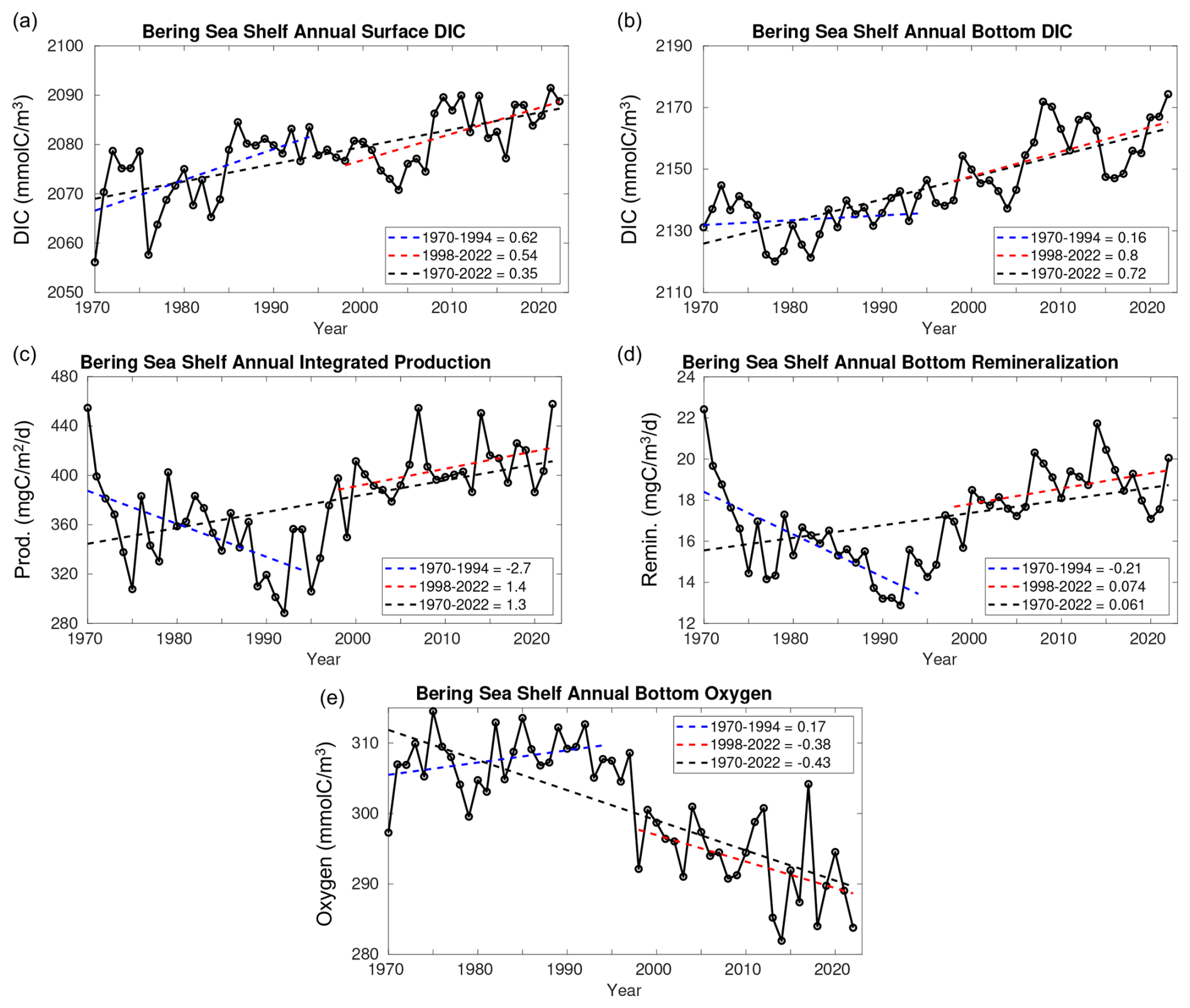
Figure 14 Time series plots of Bering Sea shelf model annual average (a) surface DIC, (b) bottom DIC, (c) depth-integrated primary productivity, (d) bottom water remineralization, and (e) bottom water oxygen concentration. Also shown are the linear trend values over three different timeframes.

Figure 6 illustrates that linear trends in Ω_arag and pH are greater at the bottom compared to the surface, especially for the CFSR-forced timeframe. Figure 14 demonstrates that this is also true for the trend in DIC, where the bottom trend over the entire model hindcast is a little over twice as strong compared to the surface. The CORE and CFSR forcing comparison illustrates that this enhanced bottom trend is a result of the CFSR-forced time series, which is a factor of ∼1.5 greater at the bottom compared to the surface for 1998–2022. Conversely, the CORE-forced surface trend is more than 3 times as strong as the bottom trend. However, extending the CORE forcing to 2003 doubles the bottom DIC trend, reducing this surface-to-bottom-trend comparison to less than a factor of 2 (Fig. S7). There are also positive trends in integrated primary production and bottom water remineralization, along with a negative trend in bottom oxygen concentrations over the entire model timeframe. Here, primary production refers to gross primary production (GPP) and remineralization encompasses all detrital remineralization and benthic excretion. Productivity and remineralization rates are both relatively high to start the model simulation, before decreasing to a minimum in the early 1990s and then steadily increasing through the remainder of the model simulation. This increase in productivity is tied to an increase in nitrate concentrations from the CORE to CFSR forcing, along with a positive trend in shortwave radiative forcing during the CFSR-forced timeframe. This leads to opposite trends in all three variables between the CORE- and CFSR-forced timeframes, with CORE trending towards lower productivity, remineralization, and higher oxygen but CFSR trending towards higher productivity, remineralization, and lower oxygen. However, the CORE trends are more affected by the relatively anomalous initial values, and the extended CORE-forced simulation also suggests a shift towards higher productivity and remineralization, though not to the same extent as the overlapping CFSR-forced years (Fig. S7). Over the entire model hindcast, productivity is strongly correlated with bottom remineralization (R=0.92) and negatively correlated with bottom oxygen ($R=-\mathrm{0.76}$).

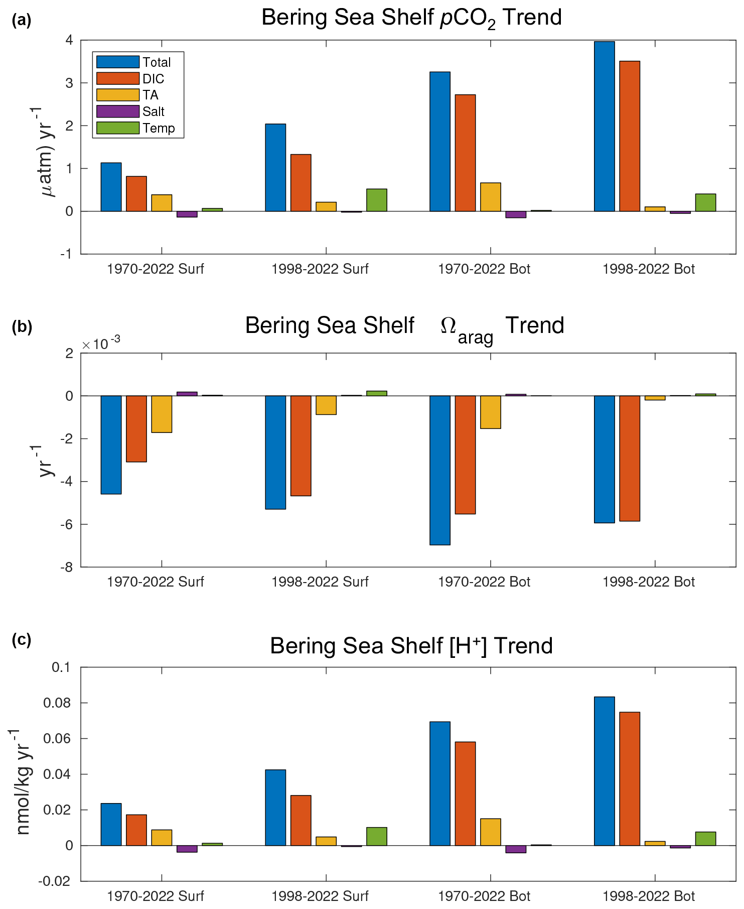
Figure 15 Taylor series decomposition of trends in pCO₂ (a), Ω_arag (b), and [H⁺] (c) for surface and bottom waters over the 1970–2022 and 1998–2022 timeframes.

To further understand the drivers behind changes in the carbonate chemistry, we also use a first-order Taylor series to decompose changes in pCO₂, Ω_arag, and [H⁺] into the four primary drivers:

$$\begin{array}{}\text{(11)}& \begin{array}{rl}\mathrm{\Delta }\mathit{\varphi }& ={\displaystyle \frac{\partial \mathit{\varphi }}{\partial \text{DIC}}}\mathrm{\Delta }\text{DIC}+{\displaystyle \frac{\partial \mathit{\varphi }}{\partial \text{TA}}}\mathrm{\Delta }\text{TA}+{\displaystyle \frac{\partial \mathit{\varphi }}{\partial \text{Salt}}}\mathrm{\Delta }\text{Salt}\\ & +{\displaystyle \frac{\partial \mathit{\varphi }}{\partial \text{Temp}}}\mathrm{\Delta }\text{Temp},\end{array}\end{array}$$

where Δϕ represents the time change in the calculated carbonate parameter (pCO₂, Ω_arag, or [H⁺]), and the four variables on the right-hand side of the equation account for the contributions of DIC, TA, salinity, and temperature, respectively. The partial derivatives are calculated through small perturbations using CO2SYS (Lewis and Wallace, 1998; Sharp et al., 2023). We employ the Taylor series decomposition for both the entire 1970–2022 timeframe and the CFSR 1998–2022 timeframe (Fig. 15). This decomposition further highlights that the OA trends are driven by increasing DIC, particularly for bottom waters. Surface carbonate trends are also driven to a lesser extent by decreasing TA over the 1970–2022 timeframe, though this effect is somewhat diminished during the more recent 1998–2022 timeframe. On this timeframe, warming temperatures emerge as a driver for surface and bottom pCO₂ and [H⁺], though they are still lower in magnitude than DIC.

4 Discussion

Our model hindcast simulates surface Ω_arag and pH trends of −0.043 and −0.014 per decade and bottom Ω_arag and pH trends of −0.066 and −0.028 per decade, respectively, from 1970–2022 for the Bering Sea shelf. This surface pH trend is comparable to the global observed mean pH decline over a similar timeframe due to ocean acidification (Lauvset et al., 2015; Ma et al., 2023). Our surface Ω_arag trend is lower than the global observed Ω_arag trend of −0.071 per decade (Ma et al., 2023), though the global high-latitude trend is more comparable to our model trend. Pilcher et al. (2022) projected that surface Ω_arag on the Bering Sea shelf would decline by −0.044 to −0.097 per decade from 2010–2100 under the RCP 4.5 and RCP 8.5 emissions scenarios, respectively, while surface pH would decline by −0.015 to −0.04 per decade. Thus, our hindcast simulation has a historical acidification rate from 1970–2022 that is comparable to the projected RCP 4.5 acidification rate. Conversely, the RCP 8.5 acidification rate is more than twice as great as our historical rate. This comparison provides context for the rate of change in carbonate chemistry that marine ecosystems have already experienced compared to the projected rate over the 21st century.

Surface trends in Ω_arag are comparable across all model timeframes, while surface trends in pH and [H⁺] are stronger over the last 25 years, reflecting a recent increase in the rate of acidification likely driven by the increased rate of atmospheric CO₂ growth. Interannual variability in surface carbonate variables also increased over the past 25 years, including the emergence of multi-year periods of sustained anomalous conditions. This is especially apparent for surface Ω_arag, with periods of relatively high (e.g., 2001–2007 and 2014–2019) and low (e.g., 2008–2013) Ω_arag conditions. This coincides with the observed warm and cold temperature “stanzas” that have emerged for the Bering Sea shelf (Stabeno et al., 2012; Stabeno and Bell 2019). For the surface and bottom, warm temperatures lead to higher Ω_arag values, while cold temperatures generate lower Ω_arag values. Pilcher et al. (2019) noted a similar phenomenon between a warm and cold temperature regime and attributed this to a combination of the thermal solubility effect on Ω_arag (i.e., cooling decreases Ω_arag) and increased fall productivity and ocean carbon uptake. In our study, thermal solubility is likely also a contributor to recent Ω_arag variability; however, surface DIC (Fig. 14a) also displays a similar pattern between warm and cold temperature regimes, suggesting the influence of changes in biogeochemistry (i.e., Pilcher et al., 2019). The warm and cold regimes also generate substantial differences in sea ice extent, which can impact the seasonal carbon cycle through changes in air–sea flux inhibition, the timing and composition of the spring phytoplankton bloom, and changes in the sea ice carbonate pump (e.g. Mortenson et al., 2020). A complete mechanistic breakdown of how the warm and cold temperature regimes impact the seasonal carbon cycle and modify background OA rates is beyond the scope of this present paper but is the focus of planned future work.

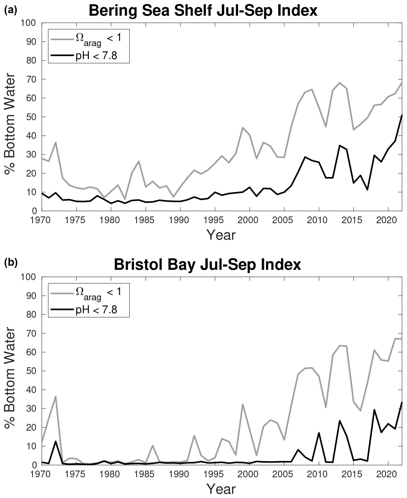
Figure 16 Time series plots of an OA indicator calculated as the spatial extent (i.e., percent of total area) of bottom waters with a July–September Ω_arag<1 (grey line) and pH <7.8 (black line). The total spatial area is the entire Bering Sea shelf for the top plot and Bristol Bay for the bottom plot.

The threat OA presents to Alaskan marine ecosystems demonstrates a clear need to develop accurate and reliable model-based OA products to support fisheries management. The recent emergence of multi-year anomalously low Ω_arag and pH conditions is significant because marine organisms may not be as resilient to longer cumulative exposure to acidic conditions (Bednarsek et al., 2022). Furthermore, OA is gradually shifting waters to a lower Ω_arag and pH baseline and reduced buffer capacity, leading to a higher rate of extreme acidity events (Burger et al., 2020) and an amplification of the seasonal cycle (Kwiatkowski and Orr, 2018). It is therefore critical to track the development of high-acidity water conditions on seasonal to annual timeframes to support practical advice within the fisheries management process. To this end, we have developed an OA index for the Eastern Bering Sea shelf using annually updated output from our model hindcast (Fig. 16). This index indicates the areal extent of the Bering Sea shelf where bottom waters are below threshold values of Ω_arag and pH from July–September. We specifically target summer bottom waters because this is when the seasonal bottom water respiration signal is greatest, thereby generating the most acidic seasonal conditions. The two biological thresholds are chosen as the aragonite saturation horizon and a pH of 7.8, which has negative effects on red king and tanner crab growth and survival (Long et al., 2013a, b, 2016). The spatial extent for both indices has greatly expanded over our model hindcast for both the entire Bering Sea shelf (Fig. 16a) and Bristol Bay (Fig. 16b) – the location of a highly valuable red king crab fishery that may already be experiencing negative effects on recruitment due to OA (Litzow et al., 2025). Prior to 2005, between 5 %–10 % of the shelf had conditions of pH <7.8, but by 2022 this jumped to more than 50 % of the shelf spatial area. Thus, locations on the shelf that had rarely or never contained these conditions in our model hindcast prior to the early 2000s now regularly experience them (Fig. 9). Currently this index, along with spatial plots highlighting pH conditions on the shelf for the current year, is included in the annual NOAA Eastern Bering Sea Ecosystem Status Report (Siddon, 2022), a key report used by the North Pacific Fisheries Management Council for setting quotas.

Modeled bottom water acidification rates on the Bering Sea shelf are substantially greater compared to the surface, particularly for pH and [H⁺]. The amplified bottom water trends emerge over the past 25 years, coinciding with a net increase in primary productivity and a subsequent increase in bottom water remineralization. This connection between surface productivity, bottom water remineralization, and relatively acidified bottom water is consistent with previous observational studies on the Bering Sea shelf (Mathis et al., 2011; Cross et al., 2014). The accumulation of anthropogenic carbon can also generate relatively greater changes in pH and [H⁺] in subsurface waters due to nonlinearities in the carbonate system (Fassbender et al., 2023), though anthropogenic carbon is not explicitly tracked in our model simulations. Our model results add to a growing body of literature suggesting that biological remineralization reduces water buffer capacity and can accelerate subsurface acidification rates (Cai et al., 2011; Feely et al., 2010; Cross et al., 2018; Kwiatkowski et al., 2020; Arroyo et al., 2022; Qi et al., 2022; Fassbender et al., 2023). Indeed, Qi et al. (2022) found accelerated OA rates in the neighboring Chukchi Sea due to enhanced subsurface biological remineralization. Previous observational studies have also noted a long-term increase in primary productivity for both the Arctic Ocean (Lewis et al., 2020) and the Bering Sea (Wang et al., 2022). Higher productivity in the Bering Sea has also been observed in warmer years (Lomas et al., 2020), though model projections suggest that overall phytoplankton biomass will decrease with future climate warming (Cheng et al., 2021). Thus, the enhanced productivity may be a transient response to recent observed warming and sea ice decline and the resulting ongoing ecological shift (Moore and Stabeno, 2015; Overland et al., 2023). Interestingly, Pilcher et al. (2022) did not find accelerated bottom water acidification rates compared to the surface in their projected OA rates for the Bering Sea shelf. These projections were generated using the same Bering10K BESTNPZ model presented in here, suggesting that the enhanced bottom OA rates in our hindcast result from the model forcing.

Here, we find that the modeled Bering Sea shelf is an annual carbon sink of 1.1–7.9 Tg C yr⁻¹, with the range resulting from the change in forcing between CORE and CFSR. Most of this carbon uptake occurs on the middle- and outer-shelf domains, while the inner-shelf domain contains some regions of net carbon efflux, mostly located near river runoff. Previous estimates for the shelf carbon sink have ranged from 2–67 Tg C yr⁻¹, and our estimate agrees with the 6.8 Tg C yr⁻¹ estimate by Cross et al. (2013) that incorporated late-fall and winter data when the shelf is typically outgassing carbon. Notably, this range is significantly less than the previous model estimate of 15–25 Tg C yr⁻¹ by Pilcher et al. (2019), which was over a much shorter timeframe (2003–2012) that only used the CFSR forcing (i.e., more comparable to our upper 7.9 Tg C yr⁻¹ estimate here). Using pCO₂ data from autonomous vehicles, Wang et al. (2022) found that Bering Sea shelf carbon uptake has increased from 1989–2019 due to an increase in primary productivity which suppressed summer pCO₂ values and generated more negative DpCO₂. Our model results present a similar mechanism (Fig. 12) but are highly uncertain as this mechanism appears to be sensitive to the switch in forcing. The substantial increase in the magnitude of the pCO_2 nonT seasonal amplitude compared to pCO_2 T may also indicate that changes in productivity and respiration are driving recent changes in the model carbon cycle and the amplified bottom water acidification rates. However, anthropogenic carbon uptake can also generate large changes in the pCO_2 nonT seasonal amplitude (Fassbender et al., 2018).

Interestingly, the strongest model trends over the past 25 years are in the off-shelf Bering Sea Basin. This region is a net annual source of carbon (Fig. 11), but the model suggests that this carbon efflux has substantially declined over the past 25 years. This region also displays divergent DpCO₂ and CO₂ flux patterns (i.e., negative DpCO₂ but positive CO₂ flux) on annual timeframes, likely due to the influence of wind speed in determining the magnitude of the flux. For example, wind speeds in the Bering Sea Basin are much stronger in winter compared to summer; thus positive winter efflux values will be greater in magnitude than negative summer influx values, generating a net positive annual average flux. However, our model results are likely more uncertain for this region because the substantially greater depths combined with our model terrain-following coordinates generate relatively deep surface grid cells, which may significantly influence the air–sea gas exchange.

A noted caveat to our model results is that the shift in atmospheric and boundary condition forcing in 1995 can lead to a shift in the system which impacts trends calculated over the entire model timeframe. For some model variables such as salinity and air–sea CO₂ flux, the impact is readily noticeable, particularly when extending the CORE forcing to 2003 (see Supplement). Conversely, the extent to which this switch impacts the trends in Ω_arag and pH is less clear. Surface Ω_arag and pH trends are largely consistent across all three timeframes, suggesting these trends are largely unaffected by the change in forcing. This result is not unexpected, given that surface acidification rates are strongly tied to the atmospheric CO₂ concentration, which is not impacted by the forcing shift. There is a moderate acceleration of the pH and [H⁺] trends over the last 25 years; however, the annual atmospheric CO₂ growth rate also increases over this same timeframe. Meanwhile, bottom Ω_arag and pH display different trends over the CORE and CFSR timeframes, with essentially no trend with the former but steep negative trends with the latter. This result may suggest that the 1970–2022 trend is not a product of a discontinuity created in 1995 by the change in forcing but rather emerges over the 1998–2022 CFSR forcing. Thus, the accelerated bottom OA rates generated by the model may be dependent on the CFSR forcing, as they are driven by enhanced productivity and remineralization that are not apparent in the CORE-forced simulation. But it does not appear that these trends are artificially generated by the switch in forcing itself. Future comparisons with newly developed model frameworks for the Northeast Pacific (i.e., Drenkard et al., 2024) may shed further light on the robustness of these trends across different models and forcing products.

It is also possible that these bottom water trends emerge over the more recent timeframe and are independent of the forcing, a conclusion supported by previous observational studies (e.g., Qi et al., 2022; Wang et al., 2022). Indeed, extending the CORE-forced simulation to 2003 generates a modest increase in bottom water acidification rates. Diagnosing the mechanism responsible for these differences in the forcing is beyond the scope of this paper, as our goal is rather to highlight which variables and trends are impacted by the transition in forcing. However, we note that the CORE atmospheric shortwave and longwave radiative forcings are slightly adjusted to agree with the CFSR radiative forcing (Kearney et al., 2020) and that water temperature comparisons between the two are comparable (Kearney, 2021). Nonetheless, this study highlights the sensitivity of the simulated carbon cycle to small shifts in surface and boundary forcing and suggests that further constraints on the spin-up and boundary condition forcing may be required as part of future model development.

5 Conclusions

We use a regional ocean biogeochemical model to simulate the Bering Sea shelf carbon cycle from 1970–2022. Over this timeframe, modeled surface waters acidify at rates comparable to those observed in the global ocean, with a slight acceleration in the trend over the past 25 years. Shelf bottom waters acidify at 2 to nearly 3 times the rate of surface waters, driven by increased productivity and subsurface respiration and remineralization. However, the magnitude of the bottom water trends may be sensitive to the timeframe and atmosphere–ocean forcing product utilized. This mechanism leads to a substantial increase in the spatial extent of summer bottom waters with Ω_arag<1 and pH conditions harmful to red king crab, including parts of the shelf where these conditions previously did not occur during our model timeframe. To facilitate tracking these conditions and support the fisheries management process, we have developed an OA index which is updated annually and presented as part of the NOAA Eastern Bering Sea Ecosystem Status Report. Lastly, we find that the modeled Bering Sea shelf is an annual carbon sink of 1.1–7.9 Tg C yr⁻¹, which is lower than a previous model estimate of 15–25 Tg C yr⁻¹ but is more consistent with the observational constraint of 6.8 Tg C yr⁻¹. The range in our estimate results from differences between the two atmospheric forcing reanalysis products, with the higher estimate driven by relatively greater carbon uptake in summer and early fall and somewhat less winter carbon efflux.