Simulating vertical phytoplankton dynamics in a stratified ocean using a two-layered ecosystem model

Phytoplankton account for around half of planetary primary production and are instrumental in regulating ocean biogeochemical cycles. Around 70 % of the oceans is characterized by either seasonal or permanent stratification. In such regions, it has been postulated that two distinct planktonic ecosystems exist, one that occupies the nutrient-limited surface mixed layer and another that resides below the mixed layer in a low-light, nutrient-rich environment. Owing to challenges observing the planktonic ecosystem below the mixed layer, it remains largely unexplored. Consequently, it is rarely characterized explicitly in marine ecosystem models. Here, we develop a simple, two-layered box model comprised of an ecosystem (nutrient, phytoplankton, and zooplankton – NPZ) in the surface mixed layer and a separate one (NPZ) in a subsurface layer below it. The two ecosystems are linked only by dynamic advection of nutrients between layers and controls on light attenuation. The model is forced with surface light (modelled from the top of the atmosphere) and observations of mixed layer depth. We run our model at the Bermuda Atlantic Time-series Study (BATS) site and compare results with a time series of more than 30 years for phytoplankton and nutrient observations. When compared with observations, the model simulates contrasting seasonal and interannual variability in chlorophyll in the two layers, reproducing the observed trends post-2011. A shoaling mixed layer post-2011, driven by ocean warming, increases light availability in both layers, which alters surface phytoplankton physiology while increasing subsurface phytoplankton biomass. Results lend support to the hypothesis that the euphotic zone of stratified systems can be described using two vertically separated planktonic ecosystems. Nevertheless, simulating the ecosystem in the subsurface layer was more challenging than the ecosystem in the surface mixed layer as less is known about model parameters and processes due to a lack of measurements, suggesting that more work is needed to study controls on subsurface planktonic communities.

1 Introduction

Phytoplankton are photosynthetic single-celled microorganisms that form the base of the oceanic food web. Their contribution to Earth's primary production is similar to terrestrial plants, accounting for approximately half of it (Longhurst et al., 1995; Field et al., 1998). These tiny organisms play a crucial role in regulating the global carbon, nitrogen, and phosphorus cycles, making them vital for Earth's climate regulation (Falkowski et al., 1998; Falkowski, 2012). Over the past century, a warming climate has been reported (Intergovernmental Panel on Climate Change, 2022), and direct (e.g. change in the carbon-to-chlorophyll ratio; C:Chl ratio) and indirect (e.g. changes in stratification) resultant impacts on phytoplankton dynamics have been identified (e.g. Winder and Sommer, 2012; Behrenfeld et al., 2016).

Around 70 % of the ocean is characterized by either seasonal or permanent stratification, with this percentage thought to be increasing with climate change (e.g. Polovina et al., 2008; Gruber, 2011; Leonelli et al., 2022). Our understanding of global surface phytoplankton dynamics is primarily based on satellite observations of chlorophyll a. However, stratified oceans often feature a relatively shallow nutrient-depleted mixed layer with a deep chlorophyll maximum (DCM) below it at depths of 80–120 m where nutrient concentrations are higher (Cullen, 1982; Fasham et al., 1985), which is hidden from satellites (Cullen, 2015; Cornec et al., 2021; Stoer and Fennel, 2024). The community of phytoplankton at the DCM is thought to contribute significantly to biogeochemical cycling in stratified waters but remains understudied (Dai et al., 2023; Viljoen et al., 2024; Stoer and Fennel, 2024). Considering the potential expansion of stratified waters with climate change (Li et al., 2020), it is important that we learn more about phytoplankton dynamics below the mixed layer.

In a stratified ocean, the euphotic zone can be theoretically divided into two vertically separated layers (Dugdale, 1967). The upper zone extends from the surface to the bottom of the mixed layer and is characterized by high light but depleted nutrients. The lower zone is between the bottom of the mixed layer and the euphotic zone and is low in light but replete in nutrients (Eppley et al., 1973; Small et al., 1987). To understand the vertical distribution of phytoplankton in stratified waters from observations collected at sea, empirical methods have been employed to partition profiles of total phytoplankton biomass into vertically separated layers. For example, Lange et al. (2018) show that high-light-adapted and low-light-adapted Prochlorococcus dominate the surface and subsurface layers, respectively, in the tropical Atlantic. Brewin et al. (2022) developed an algorithm to vertically partition phytoplankton into two communities within the upper ocean of the northern Red Sea. Recently, Viljoen et al. (2024) used this algorithm to partition phytoplankton into two vertically separated communities within the Sargasso Sea (at the Bermuda Atlantic Time-series Study – BATS – site). They found that the two communities exhibit distinct and contrasting responses to climate variability over multidecadal timescales. From 2011 to 2022, chlorophyll in the surface mixed layer showed a decreasing trend, while chlorophyll below the mixed layer and above the euphotic zone displayed an increasing trend (Viljoen et al., 2024). Understanding the mechanisms controlling the different trends in these two vertically separated phytoplankton communities may help improve predictions of future changes to the base of the marine ecosystem in stratified waters. Exploring these mechanisms requires the development of a suitable ecosystem model.

A wide range of ecosystem models are available to the biological oceanographic community, ranging from simple single nutrient–phytoplankton–zooplankton (NPZ) models (see Franks, 2002) to complex 3D models with multiple nutrient, detrital, and plankton state variables. The essence of those simple and complex ecosystem models is the nutrient–phytoplankton–zooplankton (NPZ) cycles. Based on this fundamental theory, an NPZ box model with physical forcing (mixed layer forcing) was developed by Evans and Parslow (1985), providing useful insights into phytoplankton annual cycles within the mixed layer (see Miller and Wheeler, 2012). Here, we briefly review studies using these models at BATS. Building on the earlier work of Evans and Parslow (1985), the first nitrogen-based NPZD model (where the D refers to a detrital state variable) was developed by Fasham et al. (1990), who also proposed the most widely used set of parameters for NPZ modelling. This model was later validated at BATS (Fasham, 1993), providing a foundation for further NPZD model development. Efforts have been devoted to further NPZD model development to address various scientific questions at BATS. For instance, Hurtt and Armstrong (1996, 1999) developed a model based on Fasham et al. (1990) to improve the simulation of chlorophyll concentrations and primary production dynamics through comparisons with observations. Doney et al. (1996) developed a 1D, physically coupled NPZD model, following the rationale of Fasham et al. (1990), to investigate the seasonal interaction between physics and biology in the upper ocean at BATS. Spitz et al. (1998) assimilated observations from BATS to refine parameters in the NPZD model of Fasham et al. (1990). Similarly, Schartau and Oschlies (2003) assimilated observations to derive a set of parameters that enhance the NPZD model performance in different locations in the North Atlantic Ocean, including at BATS. The NPZD model of Fasham et al. (1990) has also been coupled with a 3D physical modelling framework (Sarmiento et al., 1993) to simulate ecosystems at a regional and global scale (e.g. Oschlies and Garçon, 1999; Fennel et al., 2006; Gruber et al., 2006; Druon et al., 2010).

In this paper, we build on the early work of Dugdale (1967) and the NPZ box model of Evans and Parslow (1985) to construct a simple two-layered vertically structured NPZ model that partitions the euphotic zone of stratified waters into a surface high-light nutrient-depleted layer and a subsurface low-light nutrient-replete layer using the mixed layer depth (MLD) and base of the euphotic zone as our boundaries. Our model is built on the assumption that these two layers host two different ecosystems (Dai et al., 2023) and are linked by dynamic advection of nutrients between layers and the attenuation of light. We use data collected at BATS (a seasonally stratified site) to evaluate the construction of our model and to test whether it can capture seasonal and multidecadal variability in phytoplankton dynamics within and below the mixed layer, as well as to explain the opposite trends in these two vertically separated layers over the 2011 to 2022 period observed by Viljoen et al. (2024). A key novelty of our model is the implementation of a different set of parameters for each layer, setting it apart from existing ecosystem models. A detailed description of the model functions, parameters, and datasets used is provided in Sect. 2. The findings from sensitivity tests, model outputs, comparisons with observations, and the mechanism of different trends post-2011 in the two communities are presented in Sect. 3. Finally, Sect. 4 offers a concluding discussion of our findings.

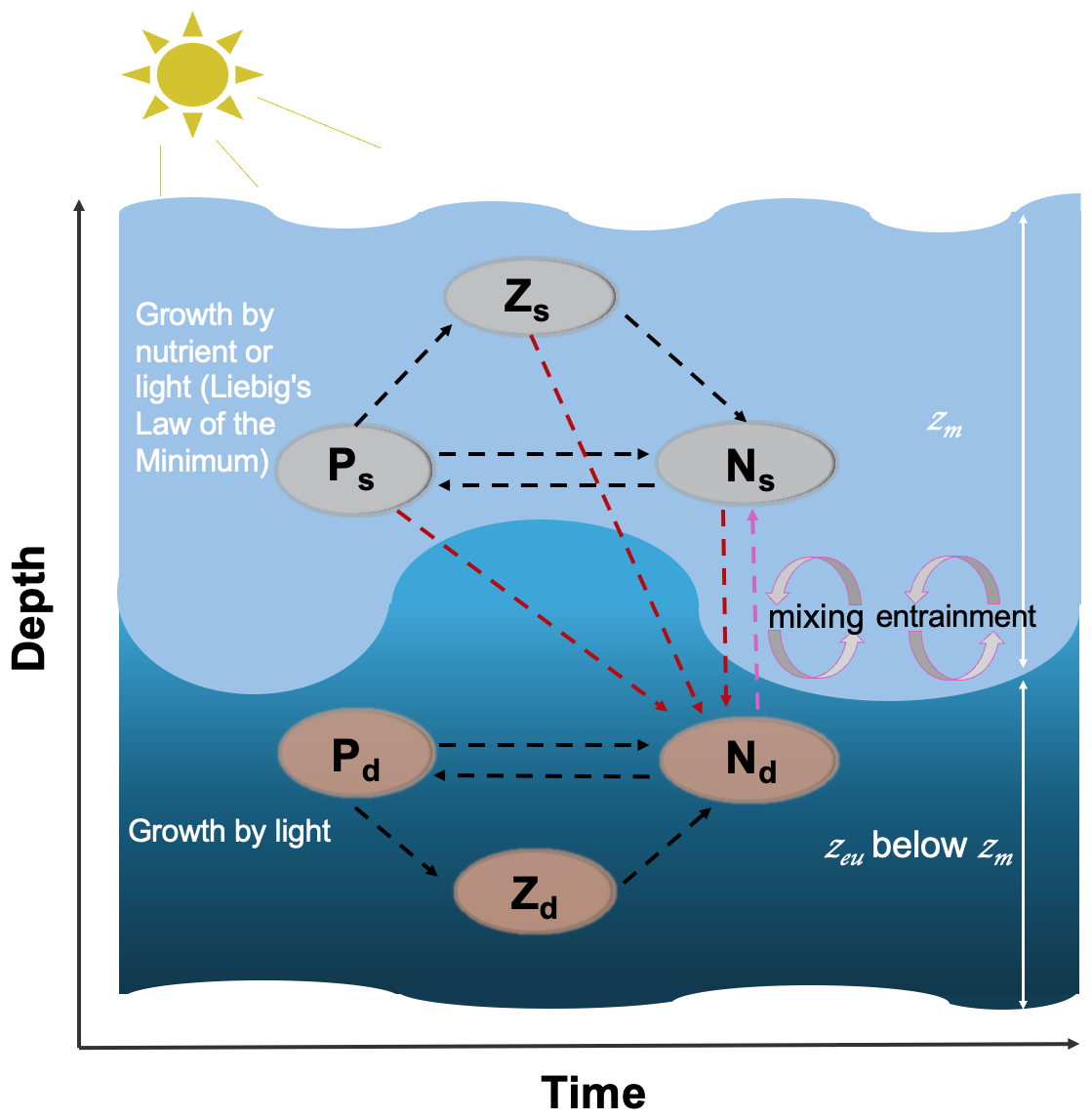
Figure 1 Schematic diagram of the two-layered ecosystem model. Light and dark blue shades represent the surface and subsurface layers, respectively. P_s, Z_s, and N_s (P_d, Z_d, and N_d) refer to the phytoplankton, zooplankton, and nutrient pools at the surface (subsurface), respectively. z_m and z_eu refer to the mixed layer depth and euphotic zone, respectively. Mixing and entrainment represent the mixing and entrainment effects driven by z_m, which is highlighted by the dashed pink line. Dashed dark red lines represent the nutrient excursion from the surface to the subsurface layer. The arrow direction denotes the direction of the nitrogen cycle.

2 Method

2.1 Model description

We present a two-layered NPZ model, building on the single-layer model of Evans and Parslow (1985). Figure 1 shows a schematic outline of our model, displaying the interaction of different nutrients, phytoplankton, and zooplankton pools. The surface layer extends from the sea surface down to the mixed layer depth (z_m), while the subsurface layer spans the bottom of z_m to the euphotic depth (z_eu) representing the depth limit of the euphotic zone (EU). In this model, z_eu is defined as the depth at which 0.0001 % of the surface light level is available (note that this is considerably deeper than the common definition of 1 % of the surface light level owing to the fact that growth by phytoplankton has been observed well below the 1 % light level (Cox et al., 2023) and to ensure that the bottom boundary of the model is always deeper than z_m). A key assumption is made in the structure of our model: the two different phytoplankton and zooplankton communities in the two layers (Dai et al., 2023) do not interact directly. Essentially, we make the assumption that each ecosystem is adapted to the environment it resides in and thus has a competitive advantage in that layer. The two ecosystems are linked only through the exchange in nutrients between the two layers as indicated by the arrows in Fig. 1. Our model is run using two forcings: z_m, which comes from observational data at the Bermuda Atlantic Time-series Study (BATS) site (see description below), and broadband surface light. Following Miller and Wheeler (2012) and Brock (1981), we model daily averaged solar radiation at the BATS site (31° N) assuming clear-sky conditions modulated by the atmospheric attenuation coefficient (Atm) and PAR fraction (f_par), and this light is attenuated through the mixed layer (with the attenuation coefficient as a function of pure water and surface chlorophyll concentration) and averaged within the mixed layer for use in surface layer modelling. Similarly, we continue to attenuate light (with the attenuation coefficient as a function of pure water and subsurface chlorophyll concentration) between z_m and z_eu, averaging it to represent the subsurface light forcing.

In the surface layer of our model, the rationale is similar to the model of Evans and Parslow (1985). The change in zooplankton concentration is controlled by grazing, mortality, and also the dilution and concentration effect due to fluctuations in z_m (see Eq. 7). A key modification we introduced is changing from a linear response of the zooplankton mortality term to a quadratic response to enhance the stability of the model (e.g. Denman, 2003; Edwards and Yool, 2000; Steele and Henderson, 1992). As in Evans and Parslow (1985), the dynamics of phytoplankton concentration are controlled by phytoplankton growth and mortality, zooplankton grazing, and the effect of z_m (see Eq. 6). For the growth term, we calculate the growth rates of nutrients and light and apply Liebig's law of the minimum to regulate phytoplankton growth (Eq. 4). Additionally, to ensure a conservative model, we modify the Evans and Parslow (1985) model by changing the asymmetric effect of z_m to a symmetric effect to ensure a conservative model. In other words, in our model, the mixed layer incorporates both dilution and concentration effects on both nutrient and phytoplankton concentrations (see Eqs. 5–6). Furthermore, as in the Evans and Parslow (1985) model, the nutrient cycle in our model is controlled by the growth and death of phytoplankton and zooplankton, as well as the mixing and entrainment effect driven by z_m (Eq. 5). For the mixing effect, we adopt a fraction of z_m (μ_m in Table 1) to represent the dynamic mixing processes between the two layers following the approach of Miller and Wheeler (2012) rather than using a fixed coefficient as in the Evans and Parslow (1985) model. Considering previously used fixed coefficients, such as 0.1 m d⁻¹ (Fasham et al., 1990) and 0.5 m d⁻¹ (Macías et al., 2007), we select μ_m=0.0055 to yield a time-mean μ_m⋅z_m of 0.3 m d⁻¹, a mid-range value that aligns well with the 0.25 m d⁻¹ used in Fennel et al. (2001).

In the subsurface layer, the dynamics of phytoplankton and zooplankton concentration adhere to principles similar to those in the surface layer. However, phytoplankton growth in the subsurface layer is simplified and dependent solely on light (Eq. 16), as light availability is significantly weaker and nutrients are substantially higher than the surface layer. The nutrient cycle in the subsurface layer (Eq. 17), however, is more complex. It involves not only the phytoplankton and zooplankton cycle in the subsurface layer but also the remineralization of nutrients from some of the dead phytoplankton and zooplankton from the surface layer (Eq. 14). In addition, nutrients in the subsurface layer are injected into the surface layer via mixing and entrainment processes. This exchange between nutrient pools in the surface and subsurface layers serves as the crucial link connecting the processes between the two layers.

In summary, the model equations for dissolved nutrient (N), phytoplankton (P), and zooplankton (Z) concentration dynamics in the surface and subsurface layers are shown as follows, with all related parameters described in Table 1.

Surface layer:

$$\begin{array}{}\text{(1)}& {\displaystyle \frac{\mathrm{d}{z}_{\mathrm{m}}}{\mathrm{d}t}}=\mathit{\zeta }\left(t\right),\text{(2)}& {\displaystyle }{\mathit{\zeta }}^{+}\left(t\right)=max(\mathrm{0},\mathit{\zeta }(t\left)\right),\text{(3)}& {\displaystyle }{\mathrm{\Phi }}_{\mathrm{s}}={\displaystyle \frac{a_{\mathrm{s}}{\mathit{ϵ}}_{\mathrm{s}}{P}_{\mathrm{c},\mathrm{s}}^{\mathrm{2}}}{a_{\mathrm{s}}+{\mathit{ϵ}}_{\mathrm{s}}{P}_{\mathrm{c},\mathrm{s}}^{\mathrm{2}}}},\text{(4)}& {\displaystyle }{G}_{\mathrm{s}}=\text{min}\left\{V_{{\max }_{\mathrm{s}}}\left(\mathrm{1}-\exp \left({\displaystyle \frac{-{\mathit{\alpha }}_{\mathrm{s}}{I}_{\mathrm{s}}}{V_{{\max }_{\mathrm{s}}}}}\right)\right),{\displaystyle \frac{V_{{\max }_{\mathrm{s}}}{N}_{\mathrm{c},\mathrm{s}}}{K_{\mathrm{s}}+N_{\mathrm{c},\mathrm{s}}}}\right\},\text{(5)}& {\displaystyle }\begin{array}{rl}{\displaystyle \frac{\mathrm{d}{N}_{\mathrm{c},\mathrm{s}}}{\mathrm{d}t}}& =-G_{\mathrm{s}}{P}_{\mathrm{c},\mathrm{s}}+{\mathit{\mu }}_p{m}_{\mathrm{s}}{P}_{\mathrm{c},\mathrm{s}}+(\mathrm{1}-{\mathit{\gamma }}_{\mathrm{s}}-{\mathit{\mu }}_g){\mathrm{\Phi }}_{\mathrm{s}}{Z}_{\mathrm{c},\mathrm{s}}\\ & +{\mathit{\mu }}_z{c}_{\mathrm{s}}{Z}_{\mathrm{c},\mathrm{s}}^{\mathrm{2}}+{\displaystyle \frac{({\mathit{\mu }}_{\mathrm{m}}{z}_{\mathrm{m}}+{\mathit{\zeta }}^{+}(t\left)\right)(N_{\mathrm{c},\mathrm{d}}-N_{\mathrm{c},\mathrm{s}})}{z_{\mathrm{m}}}}\\ & -{\displaystyle \frac{\mathit{\zeta }\left(t\right)}{z_{\mathrm{m}}}}{N}_{\mathrm{c},\mathrm{s}},\end{array}\text{(6)}& {\displaystyle \frac{\mathrm{d}{P}_{\mathrm{c},\mathrm{s}}}{\mathrm{d}t}}=G_{\mathrm{s}}{P}_{\mathrm{c},\mathrm{s}}-m_{\mathrm{s}}{P}_{\mathrm{c},\mathrm{s}}-{\mathrm{\Phi }}_{\mathrm{s}}{Z}_{\mathrm{c},\mathrm{s}}-{\displaystyle \frac{\mathit{\zeta }\left(t\right)}{z_{\mathrm{m}}}}{P}_{\mathrm{c},\mathrm{s}},\text{(7)}& {\displaystyle \frac{\mathrm{d}{Z}_{\mathrm{c},\mathrm{s}}}{\mathrm{d}t}}={\mathit{\gamma }}_{\mathrm{s}}{\mathrm{\Phi }}_{\mathrm{s}}{Z}_{\mathrm{c},\mathrm{s}}-c_{\mathrm{s}}{Z}_{\mathrm{c},\mathrm{s}}^{\mathrm{2}}-{\displaystyle \frac{\mathit{\zeta }\left(t\right)}{z_{\mathrm{m}}}}{Z}_{\mathrm{c},\mathrm{s}},\text{(8)}& {\displaystyle }{I}_k={\displaystyle \frac{V_{{\max }_{\mathrm{s}}}}{{\mathit{\alpha }}_{\mathrm{s}}}},\text{(9)}& {\displaystyle }{I}_{*}={\displaystyle \frac{I_{\mathrm{s}}}{I_k}},\text{(10)}& {\displaystyle }{\mathit{\chi }}_{\mathrm{s}}={\displaystyle \frac{I_{*}}{{\mathit{\theta }}_{\mathrm{m}}(\mathrm{1}-\exp (-I_{*}\left)\right)}},\text{(11)}& {\displaystyle }\text{Chl}{a}_{\mathrm{c},\mathrm{s}}=P_{\mathrm{c},\mathrm{s}}{Q}_{\mathrm{C}:\mathrm{N}}{\displaystyle \frac{\mathrm{1}}{{\mathit{\chi }}_{\mathrm{s}}}}{M}_{\mathrm{c}}.\end{array}$$

Subsurface layer:

$$\begin{array}{}\text{(12)}& {\displaystyle }{z}_D=z_{\mathrm{eu}}-z_{\mathrm{m}},\text{(13)}& {\displaystyle \frac{\mathrm{d}{z}_D}{\mathrm{d}t}}=\mathit{\eta }\left(t\right),\text{(14)}& {\displaystyle }\begin{array}{rl}\mathit{\varphi }& ={\displaystyle \frac{(\mathrm{1}-{\mathit{\mu }}_z)c_{\mathrm{s}}{Z}_{\mathrm{c},\mathrm{s}}^{\mathrm{2}}{z}_{\mathrm{m}}}{z_D}}+{\displaystyle \frac{{\mathit{\mu }}_g{\mathrm{\Phi }}_{\mathrm{s}}{Z}_{\mathrm{c},\mathrm{s}}{z}_{\mathrm{m}}}{z_D}}\\ & +{\displaystyle \frac{(\mathrm{1}-{\mathit{\mu }}_p)m_{\mathrm{s}}{P}_{\mathrm{c},\mathrm{s}}{z}_{\mathrm{m}}}{z_D}},\end{array}\text{(15)}& {\displaystyle }{\mathrm{\Phi }}_{\mathrm{d}}={\displaystyle \frac{a_{\mathrm{d}}{\mathit{ϵ}}_{\mathrm{d}}{P}_{\mathrm{c},\mathrm{d}}^{\mathrm{2}}}{a_{\mathrm{d}}+{\mathit{ϵ}}_{\mathrm{d}}{P}_{\mathrm{c},\mathrm{d}}^{\mathrm{2}}}},\text{(16)}& {\displaystyle }{G}_{\mathrm{d}}=V_{{\max }_{\mathrm{d}}}\left(\mathrm{1}-\exp \left(-{\displaystyle \frac{{\mathit{\alpha }}_{\mathrm{d}}{I}_{\mathrm{d}}}{V_{{\max }_{\mathrm{d}}}}}\right)\right),\text{(17)}& {\displaystyle }\begin{array}{rl}{\displaystyle \frac{\mathrm{d}{N}_{\mathrm{c},\mathrm{d}}}{\mathrm{d}t}}& =-G_{\mathrm{d}}{P}_{\mathrm{c},\mathrm{d}}+m_{\mathrm{d}}{P}_{\mathrm{c},\mathrm{d}}+(\mathrm{1}-{\mathit{\gamma }}_{\mathrm{d}}){\mathrm{\Phi }}_{\mathrm{d}}{Z}_{\mathrm{c},\mathrm{d}}\\ & +c_{\mathrm{d}}{Z}_{\mathrm{c},\mathrm{d}}^{\mathrm{2}}-{\displaystyle \frac{\mathit{\eta }\left(t\right)}{z_D}}{N}_{\mathrm{c},\mathrm{d}}\\ & -{\displaystyle \frac{({\mathit{\mu }}_{\mathrm{m}}{z}_{\mathrm{m}}+{\mathit{\zeta }}^{+}(t\left)\right)(N_{\mathrm{c},\mathrm{d}}-N_{\mathrm{c},\mathrm{s}})}{z_D}}+\mathit{\varphi },\end{array}\text{(18)}& {\displaystyle \frac{\mathrm{d}{P}_{\mathrm{c},\mathrm{d}}}{\mathrm{d}t}}=G_{\mathrm{d}}{P}_{\mathrm{c},\mathrm{d}}-m_{\mathrm{d}}{P}_{\mathrm{c},\mathrm{d}}-{\mathrm{\Phi }}_{\mathrm{d}}{Z}_{\mathrm{c},\mathrm{d}}-{\displaystyle \frac{\mathit{\eta }\left(t\right)}{z_D}}{P}_{\mathrm{c},\mathrm{d}},\text{(19)}& {\displaystyle \frac{\mathrm{d}{Z}_{\mathrm{c},\mathrm{d}}}{\mathrm{d}t}}={\mathit{\gamma }}_{\mathrm{d}}{\mathrm{\Phi }}_{\mathrm{d}}{Z}_{\mathrm{c},\mathrm{d}}-c_{\mathrm{d}}{Z}_{\mathrm{c},\mathrm{d}}^{\mathrm{2}}-{\displaystyle \frac{\mathit{\eta }\left(t\right)}{z_D}}{Z}_{\mathrm{c},\mathrm{d}},\text{(20)}& {\displaystyle }\text{Chl}{a}_{\mathrm{c},\mathrm{d}}=P_{\mathrm{c},\mathrm{d}}{Q}_{\mathrm{C}:\mathrm{N}}{\displaystyle \frac{\mathrm{1}}{{\mathit{\chi }}_{\mathrm{d}}}}{M}_{\mathrm{c}}.\end{array}$$

N_c,s, P_c,s, Z_c,s, and Chl a_c,s represent the dissolved nutrient, phytoplankton, zooplankton, and chlorophyll a concentrations at the surface layer. Similarly, N_c,d, P_c,d, Z_c,d, and Chl a_c,d represent the dissolved nutrient, phytoplankton, zooplankton, and chlorophyll a concentrations at the subsurface layer. In this model, the unit of Chl a_c,s and Chl a_c,d is mg m⁻³, whereas N_c,s, P_c,s, Z_c,s, N_c,d, P_c,d, and Z_c,d are expressed in nitrogen units, mmol N m⁻³. Here, Φ_s and Φ_d represent the grazing at the surface and subsurface layer, respectively, which share the same “Holling Type III” response (Denman and Peña, 2002) but with different parameters at different layers. The term ϕ represents the influence of the export production from the surface layer to the subsurface layer nutrient pool, and G_s shows the growth rate of the phytoplankton at the surface, determined by the processes most limiting to surface light ($V_{{\max }_{\mathrm{s}}}(\mathrm{1}-\exp (\frac{-{\mathit{\alpha }}_{\mathrm{s}}{I}_{\mathrm{s}}}{V_{{\max }_{\mathrm{s}}}}\left)\right)$) or nutrients ($\frac{V_{{\max }_{\mathrm{s}}}{N}_{\mathrm{c},\mathrm{s}}}{K_{\mathrm{s}}+N_{\mathrm{c},\mathrm{s}}}$) (Michaelis–Menten uptake, Franks, 2002). However, at the subsurface layer, the growth of phytoplankton (G_d) is set to be only limited by subsurface light (I_d). The thickness of the subsurface layer is represented as z_D.

To calculate the surface chlorophyll concentration (Chl a_c,s) in this model, we convert phytoplankton from nitrogen units in moles to carbon units in milligrams (mg) by multiplying by the molecular weight of carbon (M_c in Table 1) and the Redfield ratio (Q_C : N in Table 1). Then, we convert the carbon to chlorophyll using the surface carbon-to-chlorophyll ratio (χ_s) following the Eqs. (8)–(10) originating from Geider et al. (1997) and Jackson et al. (2017), where θ_m is the maximum chlorophyll-to-carbon ratio and I_* is dimensionless irradiance. According to Jackson et al. (2017), a suitable value for θ_m at the surface is 0.01. The dimensionless irradiance I_* is defined by Eq. (9), where I_s is the surface layer photosynthetically active radiation and I_k is defined as the ratio of maximum chlorophyll-normalized production over the chlorophyll-normalized initial slope of the photosynthesis irradiance curve (Jackson et al., 2017). Since our model does not include chlorophyll-normalized parameters, we approximate I_k as $\frac{V_{{\max }_{\mathrm{s}}}}{{\mathit{\alpha }}_{\mathrm{s}}}$ to calculate χ_s.

To calculate the subsurface chlorophyll concentration (Chl a_c,d), we followed a similar method as calculating Chl a_c,s, but used a fixed C:Chl ratio in the subsurface layer (χ_d). According to Viljoen et al. (2024), χ_d tends to be stable at the subsurface and shows a lower value than the surface layer. Thus we fixed χ_d as 156, half of the modelled time-mean χ_s, which also falls in the range of 1–226 observed by Viljoen et al. (2024).

Miller and Wheeler (2012)Miller and Wheeler (2012)Fasham et al. (1990)Fasham et al. (1990)Uitz et al. (2008)Anugerahanti et al. (2020)Anugerahanti et al. (2020)Kantha (2004)Anugerahanti et al. (2020)Anugerahanti et al. (2020)Doney et al. (1996)Anugerahanti et al. (2020)Anugerahanti et al. (2020)Anugerahanti et al. (2020)Hurtt and Armstrong (1999)Fasham et al. (1990)Fasham et al. (1990)Schartau and Oschlies (2003)Fasham et al. (1990)Oschlies and Garçon (1999)Oschlies and Garçon (1999)Pasquero et al. (2005)Pasquero et al. (2005)Pasquero et al. (2005)Pasquero et al. (2005)Fennel et al. (2001)Uitz et al. (2008)Schartau and Oschlies (2003)Schartau and Oschlies (2003)Schartau and Oschlies (2003)Schartau and Oschlies (2003)Schartau and Oschlies (2003)Schartau and Oschlies (2003)Schartau and Oschlies (2003)Jackson et al. (2017)Redfield (1958)

Table 1 Parameters used in our two-layered NPZ model, as well as their meanings, values, units, and supporting references. P/I: photosynthesis–irradiance.

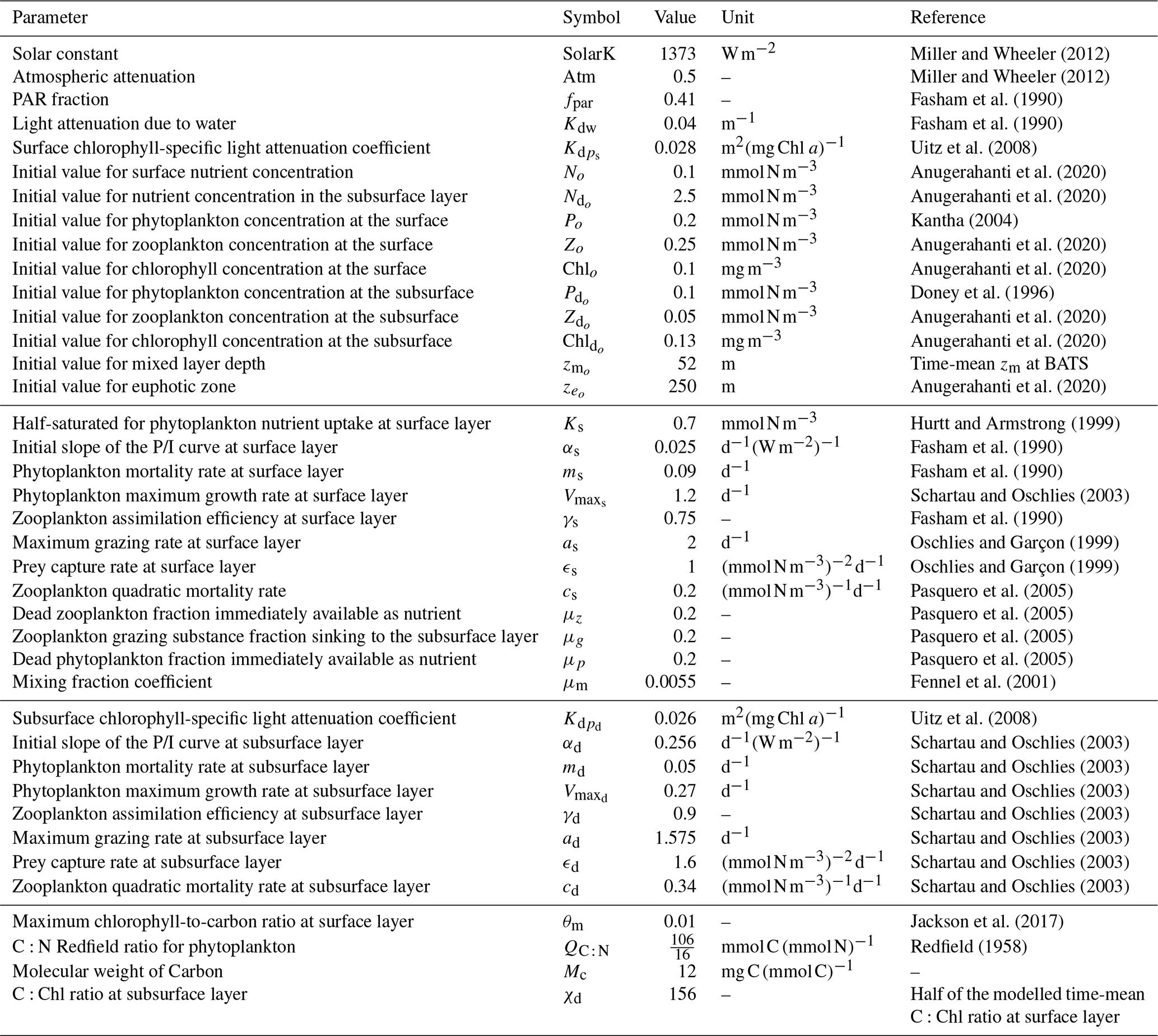
2.2 Model parameterization

Table 1 summarizes the parameters used in our model, as well as their meanings, values, units, and supporting references. In this two-layer NPZ model, most of the basic parameters (f_par, K_dw, α_s, m_s, and γ_s) at the surface come from Fasham et al. (1990), which forms the most widely used values for NPZ modelling. K_dw and $K_{\mathrm{d}{p}_{\mathrm{s}}}$ are parameters used to calculate the total attenuation coefficients ($K_{{\mathrm{d}}_{\mathrm{s}}}$) at the surface layer (see Eq. 21) such that

$$\begin{array}{}\text{(21)}& K_{{\mathrm{d}}_{\mathrm{s}}}=K_{\mathrm{dw}}+K_{\mathrm{d}{p}_{\mathrm{s}}}\cdot \text{Chl}{a}_{\mathrm{c},\mathrm{s}},\end{array}$$

where K_dw refers to the attenuation of pure water and $K_{\mathrm{d}{p}_{\mathrm{s}}}$ is the chlorophyll-specific light attenuation at the surface. Similarly, K_dw and $K_{\mathrm{d}{p}_{\mathrm{d}}}$ are parameters used to calculate the total attenuation coefficients ($K_{{\mathrm{d}}_{\mathrm{d}}}$) at the subsurface layer (see Eq. 22) such that

$$\begin{array}{}\text{(22)}& K_{{\mathrm{d}}_{\mathrm{d}}}=K_{\mathrm{dw}}+K_{\mathrm{d}{p}_{\mathrm{d}}}\cdot \text{Chl}{a}_{\mathrm{c},\mathrm{d}},\end{array}$$

where $K_{\mathrm{d}{p}_{\mathrm{d}}}$ is the chlorophyll-specific light attenuation at the subsurface. In this model, we use different values for $K_{\mathrm{d}{p}_{\mathrm{s}}}$ and $K_{\mathrm{d}{p}_{\mathrm{d}}}$ as field studies have shown that the chlorophyll-specific attenuation of phytoplankton changes vertically in stratified waters (Uitz et al., 2008). We approximate the chlorophyll-specific light attenuation from the chlorophyll-specific absorption coefficient of phytoplankton derived by Uitz et al. (2008), making $K_{\mathrm{d}{p}_{\mathrm{s}}}=\mathrm{0.028}$ m² (mg Chl a)⁻¹ and $K_{\mathrm{d}{p}_{\mathrm{d}}}=\mathrm{0.026}$ m² (mg Chl a)⁻¹.

The initial values for surface phytoplankton (P_o) and chlorophyll (Chl_o) concentrations are set to 0.2 mmol N m⁻³ and 0.1 mg m⁻³ based on observations at BATS reported by Kantha (2004) and Anugerahanti et al. (2020), respectively. Furthermore, N_o is set to 0.1 mmol N m⁻³, which is the average value of in situ NO₃ observations at BATS from 1998–2007 (Anugerahanti et al., 2020). Observational data for zooplankton at different depths are more challenging to find. To keep consistency, we chose the Z_o=0.25 mmol N m⁻³ based on the experiment that produces phytoplankton and nutrient results closely matching in situ data (PPE in Fig. 2 in Anugerahanti et al., 2020). The initial value of the mixed layer depth ($z_{{\mathrm{m}}_o}$) is set to be 52 m, the time-mean value of z_m from 1990 to the end of 2022 at the BATS location (data are described below). Given that the time-mean chlorophyll tends to be near zero at 250 m (Anugerahanti et al., 2020), we define the initial value of the euphotic zone ($z_{e_o}$) as 250 m.

Regarding the initial values at the subsurface layer, $P_{{\mathrm{d}}_o}$ is challenging to determine since few studies present phytoplankton concentrations in mmol N m⁻³ at various depths. Nevertheless, based on the vertical phytoplankton concentration profile from 0 to 250 m at the BATS location simulated by the NPZD model from Doney et al. (1996), the phytoplankton concentration at 50–250 m ranges from approximately 0.05 to 0.15 mmol N m⁻³. Consequently, $P_{{\mathrm{d}}_o}$ is given as 0.1 mmol N m⁻³, in the centre of that range. Given that time-mean Chl a_c,d varies from 0.01 to 0.25 mg m⁻³ between 50–250 m (Anugerahanti et al., 2020), ${\text{Chl}}_{{\mathrm{d}}_o}$ is defined in the centre of the range at 0.13 mg m⁻³. For $Z_{{\mathrm{d}}_o}$ and $N_{{\mathrm{d}}_o}$, we follow the same methodology used to determine initial values in the surface layer but select values at around 200 m from Anugerahanti et al. (2020).

We employ the most traditional values for the maximum grazing rate (a_s) and prey capture rate (ϵ_s) in the surface layer, as outlined by Oschlies and Garçon (1999). The zooplankton quadratic mortality rate (c_s) and the coefficients related to the excretion of the nutrients from the first to the second layer (μ_z, μ_g, and μ_p) are adopted from Pasquero et al. (2005), which are also used in other literature (e.g. Sandulescu et al., 2007; Yaya et al., 2021). Given that our hypothesis is tested at the BATS location, characterized by a seasonally stratified ocean, we adjusted the initial values of $V_{{\max }_{\mathrm{s}}}$ and K_s to reflect the conditions specific to this area. Schartau and Oschlies (2003) show that $V_{{\max }_{\mathrm{s}}}$ has a strong seasonal cycle at the BATS location ranging from around 1 to 1.4 d⁻¹. Accordingly, we select $V_{{\max }_{\mathrm{s}}}=\mathrm{1.2}$ d⁻¹, an average value of this range. Given the range of 0.45–0.91 mmol N m⁻³ for the half-saturation constant for phytoplankton nutrient uptake at the surface layer (K_s) at BATS, as reported by Hurtt and Armstrong (1999), we adopt K_s=0.7 mmol N m⁻³, a midpoint of that range.

In the subsurface layer, given that no study has employed different parameters at different layers in an NPZ model, it is challenging to adjust the parameters based on existing literature. However, as we know the light availability should be much lower at the subsurface, which implies that the initial slope of the photosynthesis irradiance curve (α_d) and phytoplankton maximum growth rate ($V_{{\max }_{\mathrm{d}}}$) at the subsurface may be higher and lower than the surface, respectively (Fasham, 1993). Schartau and Oschlies (2003) provide a set of parameters by assimilating observational data at the BATS location, including a higher α_d and lower $V_{{\max }_{\mathrm{d}}}$, which are used in our model. To maintain consistency, we use their parameters for the rest of our subsurface parameters.

2.3 Model sensitivity analysis

To determine the sensitivity of model parameters, we conducted a series of experiments. First, the model was run from 1990 to 2022 with the parameters listed in Table 1 with the chlorophyll, zooplankton, and nutrient concentration stocks at the surface and subsurface layers saved (default run). Next, the model was run again with each parameter (except for SolarK, K_dw, Q_C : N, and M_c, which are well-known) individually increased and decreased by 10 % while keeping the remaining parameters fixed (sensitivity runs). We then calculate the time-mean values of each state variable in sensitivity runs and the default run and computed the ratios by dividing the former by the latter. Eventually, these ratios construct a general range (Λ), illustrating how the mean values deviate from the default run in response to a 10 % change (increase or decrease) in each parameter in Table 1.

2.4 Model validation

Ship-based data from BATS (1990–2022) were used to calculate integrated stocks of chlorophyll and dissolved NO₂ + NO₃, as well as mixed layer depth (z_m) used in this study, following the methodology outlined by Viljoen et al. (2024). Temperature profiles from conductivity, temperature, and depth (CTD) casts (Johnson et al., 2024) were used to compute z_m, specifically for profiles with concurrent temperature and salinity data that included measurements in the surface (<11 m). The z_m was calculated using the temperature-based algorithm implemented in the holteandtalley Python package (Holte and Talley, 2009). Chlorophyll a concentrations were extracted from high-performance liquid chromatography (HPLC) pigment data (Johnson et al., 2023a), including only profiles with a minimum of six depth measurements and coincident CTD and particulate organic carbon (POC) bottle data. Dissolved inorganic nitrogen (DIN) measurements were obtained from nitrate + nitrite profiles on the BATS data server (http://bats.bios.edu/bats-data/, last access: 18 July 2023). Only DIN profiles with at least six measurements in the upper 350 m and that aligned with selected HPLC chlorophyll a and temperature profiles were used. All CTD, HPLC, and DIN data were restricted to profiles within a 0.5° latitude and longitude box around the BATS site.

We ran our model with the parameters in Table 1 from 1 January 1990 to 31 December 2022 in a daily time step at BATS to derive a chlorophyll and nutrient concentration daily time series. This model was not spun up, but it stabilized within 1 month, which indicates that the model output became comparable with observations as of 1 February 1991. To estimate the stocks of chlorophyll and nutrients in the model, we multiplied the vertically averaged concentration in each layer by the thickness of each layer. The thicknesses of the surface and subsurface layer are z_m and z_D (see Eq. 12), respectively. Next, to compare model output with observations, we used the observational chlorophyll and nutrient integration above z_m time series at BATS from Viljoen et al. (2024) as referenced observational stocks at the surface layer, as we use the same z_m, which is also used as the bottom boundary for the surface layer in the model. For the subsurface layer stock calculation, we first integrate observational chlorophyll and nutrient concentrations at BATS from z_m to z_k (z_k refers to the deepest depth level of the measurements at each time step just above z_eu). This integration is then divided by the (z_k minus z_m) to obtain the averaged concentration between z_m and z_k. This average concentration was used as a representative value for the water column from z_m to z_eu and then multiplied by the model subsurface thickness (z_D) to derive the subsurface phytoplankton and nutrient stocks.

In addition to the time series of stocks, we also calculate a time-mean climatology of surface and subsurface chlorophyll and nutrient stocks. To determine the relationship between observational and model outputs, we calculate Spearman's correlation coefficient (Corr.) and the significance level (p) using only the time steps where data are available for both observations and model outputs.

2.5 Data deseasonalization and trend analysis

To compare model estimates of interannual variability with observations, we first resampled the daily time series from the model to be monthly time series using the monthly median as described in Viljoen et al. (2024). To keep the same method that Viljoen et al. (2024) used, we dealt with missing values in observations using a median climatology. Finally, we decompose the surface and subsurface chlorophyll stocks in the model and observations and extract the deseasonalized time series, following the same method applied in Viljoen et al. (2024), using the Python function MSTL from the statsmodels.tsa.seasonal package, with a period of 12 representing the months of the year. We then calculate the Spearman's correlation coefficient (Corr.) and significance (p) of the deseasonalized time series between the model and observations.

To utilize this model to determine the drivers of the different post-2011 trends at the surface and subsurface layer (Viljoen et al., 2024), we first resample daily surface and subsurface light, the surface C:Chl ratio, and the surface and subsurface chlorophyll, phytoplankton, zooplankton, and DIN concentration from the model to a monthly time series and decomposed it to produce deseasonalized data following the method described above. To examine the trend of each time series post-2011, linear regression analysis (Python sklearn.linear_model.LinearRegression) is first applied to all extracted deseasonalized data described above (including modelling and observational time series) over 2011–2022. Based on this linear regression, we extract the slope (S) of the trend between 2011 (including 2011) and the end of 2022 and obtain the p value to examine the significance of the trend. Also, according to the linear regression, we calculate the percentage change (Δ) in the fitted model as the relative difference between the start and end values of the model fit between 2011 and 2022.

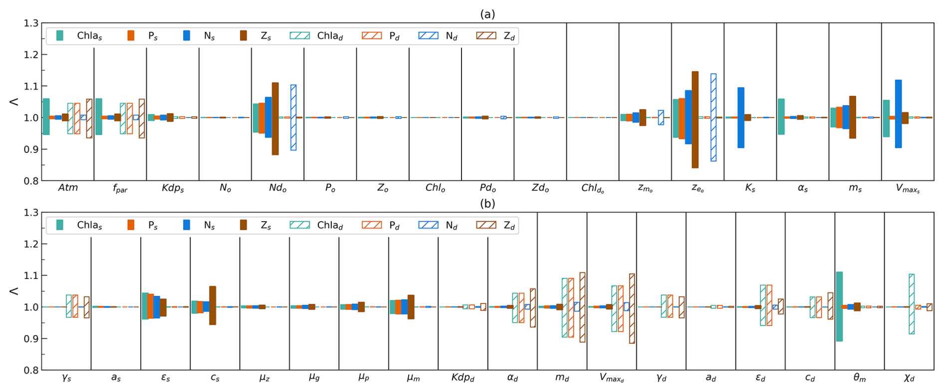
Figure 2 (a–b) Sensitivity of model output (difference in time mean, denoted Λ) for surface-layer-integrated chlorophyll (Chl a_s), phytoplankton (P_s), nutrients (N_s), and zooplankton (Z_s), as well as subsurface-layer-integrated values (Chl a_d, P_d, N_d, Z_d), when increasing and decreasing each parameter from Table 1 (except for SolarK, K_dw, Q_C : N, and M_c) by 10 % individually whilst keeping the remaining values fixed.

3 Results

3.1 Model sensitivity

The range of two values (Λ) for each parameter is shown in Fig. 2. In the bar plot, the more Λ varies from 1.0, the greater the difference between the adjusted and default model outputs. Among the eight state variables (Chl a_s, P_s, N_s, Z_s, Chl a_d, P_d, N_d, Z_d), N_s show large ranges (>0.94–1.06) when varying four parameters ($N_{{\mathrm{d}}_o}$, $z_{e_o}$, K_s, and $V_{{\max }_{\mathrm{s}}}$). This suggests that surface nutrient stocks are sensitive to changes in these parameters, reflecting their dependence on initial deep ocean nutrient stocks and surface phytoplankton growth.

Following N_s, the chlorophyll (Chl a_d), phytoplankton (P_d), and zooplankton (Z_d) stocks in the subsurface layer exhibit the next highest sensitivity in this model. They show a tendency to be sensitive to changes in parameters at the subsurface layer (notably m_d, $V_{{\max }_{\mathrm{d}}}$, and ϵ_d) and the light attenuation coefficient in the atmosphere (Atm and f_par). In addition, Chl a_d is also sensitive to a change in χ. This suggests that the net growth of phytoplankton and light play the most important role in modulating Chl a_d, P_d, and Z_d, and the subsurface C:Chl ratio has a large impact on Chl a_d. In contrast, the surface chlorophyll (Chl a_s) stock is sensitive primarily to the change in parameters at the surface layer. The key parameter θ_m in the photo-acclimation model also plays an important role in determining Chl a_s. Compared to Chl a_s, surface zooplankton (Z_s) and phytoplankton stocks (P_s) tend to be more stable, primarily sensitive to $N_{{\mathrm{d}}_o}$, $z_{e_o}$, and m_s. This indicates that the initial assumption of the deep-ocean nutrient stocks and the death of phytoplankton have a impact on Z_s and P_s. N_d tends to be the most stable parameter, resilient to the changes in all parameters except for $N_{{\mathrm{d}}_o}$ and $z_{e_o}$. However, notably, the range of Λ in N_d is the second largest (0.86–1.14) when varying $z_{e_o}$ compared to Λ in other parameters. These findings indicate that changes in most of the parameters hardly impact N_d. However, the determination of $N_{{\mathrm{d}}_o}$ and $z_{e_o}$ is pivotal to good N_d estimation.

From a parameter perspective, this model is not sensitive to changes in the μ_z, μ_g, μ_p, and initial values except for $z_{e_o}$ and $N_{{\mathrm{d}}_o}$. This indicates that this model is not sensitive to changes in the excursion process from the surface to subsurface layer and changes in most of the initial values. However, $z_{e_o}$ and $N_{{\mathrm{d}}_o}$ show large ranges of Λ for all state variables at the surface layer (especially for surface zooplankton stock) and subsurface nutrient stock. This highlights the importance of getting initial nutrient stock conditions in the subsurface layer right.

Table 2 The concentration of chlorophyll, phytoplankton, zooplankton, and nutrients at two layers in the model. Chl a_c,s, P_c,s, Z_c,s, and N_c,s represent the chlorophyll a, phytoplankton, zooplankton, and DIN vertically averaged concentration in the surface layer time series, and Chl a_c,d, P_c,d, Z_c,d, and N_c,d represent the chlorophyll a, phytoplankton, zooplankton, and DIN vertically averaged concentration between the bottom of the z_m and z_eu time series from the model. The time mean ($\overline{R}$), minimum (R_min), and maximum (R_max) of these time series are presented. The units of each parameter are shown in square brackets. The statistics are based on the time series from 1 February 1990 to 31 December 2022.

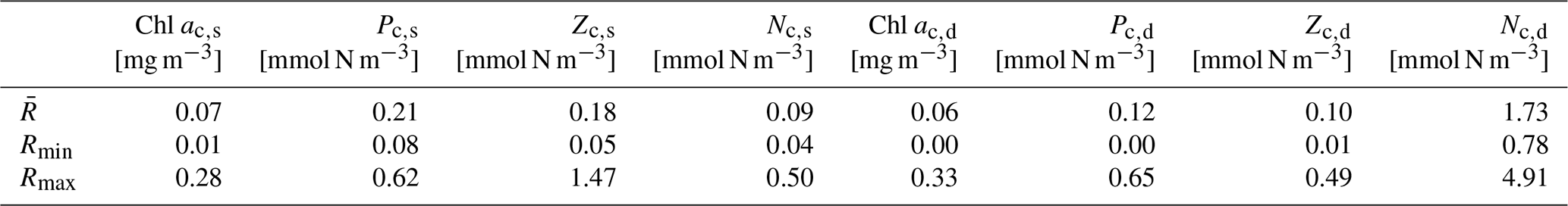
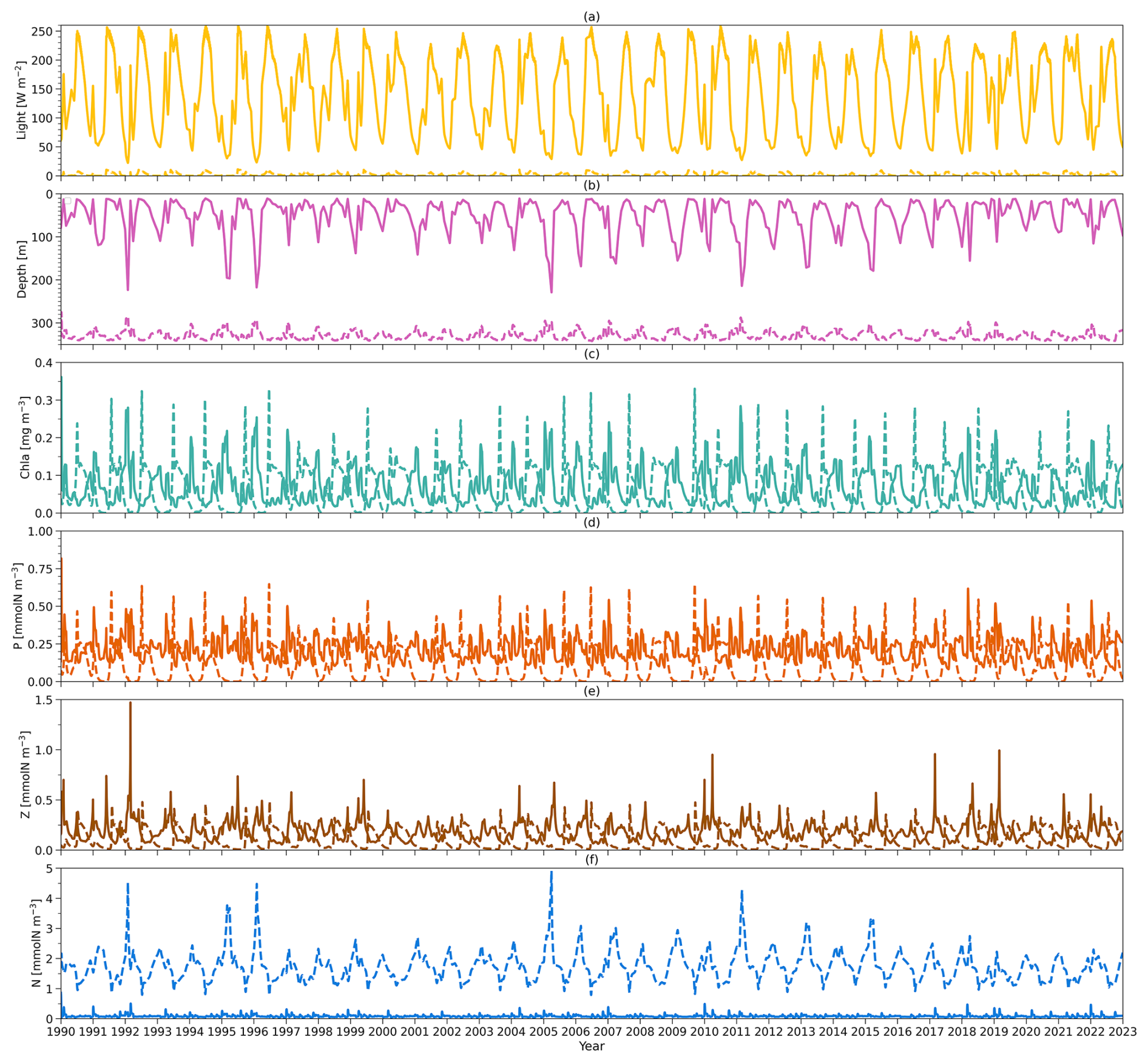
Figure 3 (a) Solid (dashed) yellow lines refer to vertically averaged light within the surface (subsurface) layer in the model from 1990 to 2022. (b) Solid and dashed pink lines represent the observational z_m from BATS and z_eu simulated by the model, respectively, from 1990 to 2022. (c) Solid (dashed) lines indicate the model output of the chlorophyll a concentration vertically averaged within the surface (subsurface) layer from 1990 to 2022. (d) As in (c) but for phytoplankton concentration. (e) As in (c) but for zooplankton concentration. (f) As in (c) but for nutrient concentration.

3.2 Model forcing, output, and validation

Figure 3 shows the daily forcing and outputs of the two-layered model from 1990 to 2022. The light forcing at the surface (solid yellow line) and subsurface layers (dashed yellow line) is presented in Fig. 3a. Surface light ranges from 22 to 262 W m⁻² with the minimum in winter and the peak during summer. Subsurface light shows a similar seasonality though its intensity decreases, ranging from 0 to 11 W m⁻². The mixed layer depth (z_m) forcing from observations at BATS is shown in Fig. 3b (solid pink line). z_m also has a strong seasonality, with a minimum in summer and a maximum in winter. It can be as shallow as 10 m during summer and as deep as 200 m in winter. Below z_m, the euphotic zone (z_eu) estimated from the model is shown in Fig. 3b (dashed pink line), which shows a contrasting seasonality to z_m with the shallowest z_eu in winter and deepest z_eu in summer.

Figure 3c–f illustrate the vertically averaged concentrations of phytoplankton, zooplankton, and dissolved inorganic nitrogen (DIN) within the surface layer in the model (solid lines). In the initial month of the simulation (January 1990), the model exhibits instability, reflected by a spike value (0.8 mmol N m⁻³) in the phytoplankton concentration at the surface layer. Nevertheless, the model quickly stabilizes. Consequently, the statistical analysis presented here is based on model outputs from 1 February 1990 to the end of 2022 (Table 2). Surface chlorophyll a, phytoplankton, zooplankton, and DIN surface concentrations show ranges of 0.01–0.28 mg m⁻³, 0.08–0.62 mmol N m⁻³, 0.05–1.47 mmol N m⁻³, and 0.04–0.5 mmol N m⁻³, respectively, with mean values of 0.07 mg m⁻³, 0.21 mmol N m⁻³, 0.18 mmol N m⁻³, and 0.09 mmol N m⁻³ for chlorophyll, phytoplankton, zooplankton, and DIN concentration (Table 2). This model also displays seasonality in these state variables. During winter and spring, nutrient availability increases in the surface layer (with a deeper mixed layer), resulting in slightly higher concentrations of phytoplankton and chlorophyll. This is followed by a maximum zooplankton concentration in the subsequent month driven by grazing on phytoplankton. These findings reveal that, at the surface layer, the phytoplankton concentration remains relatively stable over the year but is slightly higher in spring driven by the increase in DIN and light availability, providing somewhat more food to zooplankton.

Compared to the surface layer, the magnitude of the subsurface chlorophyll (Fig. 3c, dashed green line) concentration is very similar, reflected by a similar range of 0–0.33 mg m⁻³ with a time mean of 0.06 mg m⁻³ (Table 2). However, subsurface phytoplankton (Fig. 3d, dashed orange line) and zooplankton (Fig. 3e, dashed brown line) concentrations decrease to ranges of 0–0.65 and 0.01–0.49 mmol N m⁻³, respectively, with the time-mean values of 0.12 and 0.10 mmol N m⁻³, respectively (Table 2). In addition, phytoplankton and zooplankton concentrations in the subsurface layer show strong seasonality, in contrast to that in the surface layer. When the chlorophyll and phytoplankton concentration in the subsurface layer reaches the minimum, the surface concentration tends to be higher and vice versa. Minimum chlorophyll concentration in the surface layer, coupled with the shallowest z_m and highest surface light in summer, creates conditions of higher light availability in the subsurface layer, increasing phytoplankton growth. This increased growth in subsurface phytoplankton subsequently supports zooplankton growth.

The DIN concentration in the subsurface layer (Fig. 3f, dashed blue line) ranges from around 0.78 to 4.91 mmol N m⁻³ with a time-mean value of 1.73 mmol N m⁻³, which is notably higher than that in the surface layer (see Table 2). This difference in the two DIN pools and the distinctive light environments between the two layers (Fig. 3a) highlight the different conditions for phytoplankton growth: the surface layer is characterized by depleted nutrients but adequate light, whereas the subsurface layer is dominated by weak light but abundant nutrients. These conditions likely create two distinct environments to which different phytoplankton communities have adapted.

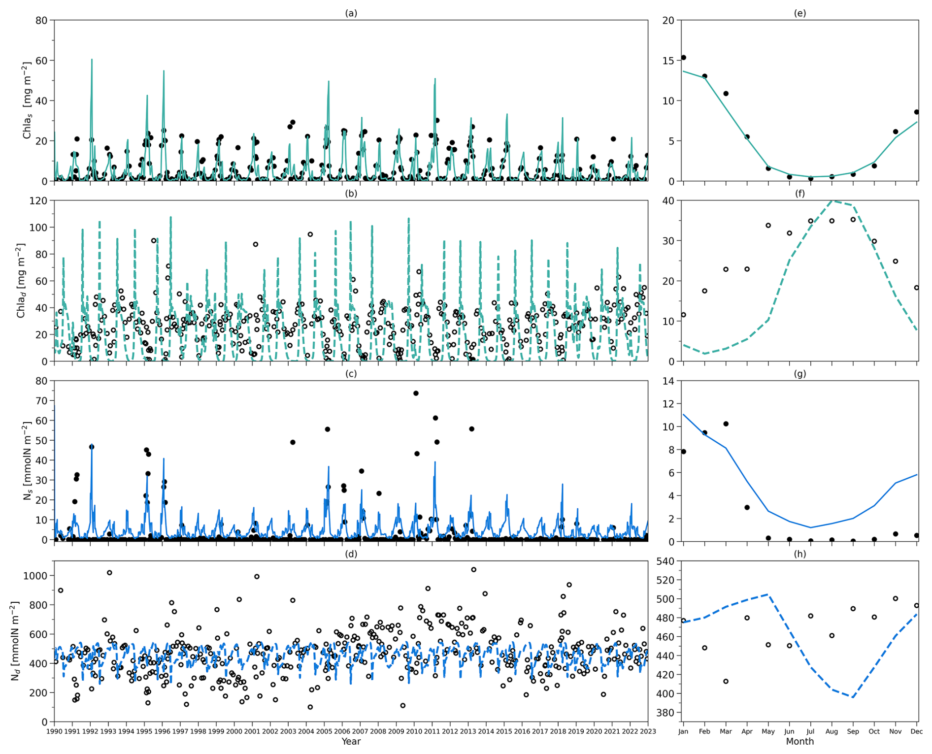
Figure 4 (a) Daily chlorophyll stocks at the surface layer from the model (solid green line) and observations (dark solid dots) from 1990 to 2022. (b) Daily chlorophyll stocks at the subsurface layer from the model (dashed green line) and observations (hollow dark dots) from 1990 to 2022. (c) Daily nitrogen stocks at the surface layer from the model (solid blue line) and observations (hollow dark dots) from 1990 to 2022. (d) Daily nitrogen stocks at the subsurface layer from the model (dashed blue line) and observations (hollow dark dots) from 1990 to 2022. (e–h) As in (a–d) but for their time-mean monthly climatology.

Table 3 The integration of chlorophyll and nutrients from the model and observations, as well as their relationships. Chl a_s and N_s represent the Chl a and DIN integration time series within the surface layer. Chl a_d and N_d represent the Chl a and DIN integration time series between the bottom of the z_m and z_eu. $\overline{R}$, R_min, R_max, and σ represent the time mean, minimum, maximum, and standard deviation of each time series described above. The correlation coefficient, Corr.(model, obs), shows the relationship between the full signal of each time series in the model and observation; its corresponding p value is shown in parentheses. $\widehat{R_{\min }}$ and $\widehat{R_{\max }}$ represent the minimum and maximum of the time-mean monthly climatology of Chl a_s, Chl a_d, N_s, and N_d. M_min and M_max represent the month when $\widehat{R_{\min }}$ and $\widehat{R_{\max }}$ are reached. Values are shown for the model and observations (in parenthesis). The units of each parameter are shown in square brackets, except for Corr.(model, obs), which does not have units. The statistics of the full time series are based on the time series from 1 February 1990 to 31 December 2022.

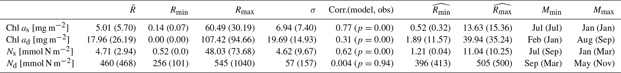
To compare the model output with observational data from BATS, chlorophyll and DIN stocks are calculated at each layer. Figure 4a first shows the chlorophyll integrated from the sea surface to z_m from model output (green line) and observations (solid dark dots) spanning 1990 to 2022. When masking the observational missing values in modelling output, the observations and modelling output show a strong and significant correlation (Corr. = 0.77, Table 3). After the model stabilizes (as of 1 February 1990), modelled chlorophyll ranges from 0.14 to 60.49 mg m⁻², which is higher than the observed range of 0.07–30.19 mg m⁻² as shown in Table 3. However, modelled surface chlorophyll stock shows a similar time-mean value of 5.01 mg m⁻² as in observations (5.7 mg m⁻²). Also, the standard deviation from the model (6.94 mg m⁻²) exhibits strong similarity to observations (7.4 mg m⁻²). These findings indicate that the two-layered model successfully simulates the surface chlorophyll stock dynamics, including the intra-annual variability.

Figure 4e compares monthly averaged chlorophyll stocks above the z_m from modelling output (solid green line) and observations (solid dark dots). Observed chlorophyll stocks show a strong seasonal variability with a maximum (15.36 mg m⁻²) in January and a minimum (0.32 mg m⁻²) in July. The model mirrors this seasonal cycle by showing a similar peak (13.63 mg m⁻²) in January and a minimum (0.52 mg m⁻²) in July (Table 3).

Figure 4b shows the subsurface chlorophyll integrated from z_m to z_eu from the model (dashed green line) and observations (hollow black dots). The modelling and observational time series also show a significant positive correlation (Corr. = 0.31) although lower than the surface layer. Table 3 shows that subsurface chlorophyll integration in the model ranges from 0 to 107.42 mg m⁻², closely matching the observed range of 0 to 94.66 mg m⁻². However, in general, the model estimates relatively lower chlorophyll stocks in the subsurface layer compared to observations, as indicated by a lower time-mean value of 17.96 mg m⁻² in the model than 26.19 mg m⁻² observed at BATS. Different from the mean values, the standard deviation from the model (19.69 mg m⁻²) is higher than in observations (14.93 mg m⁻²), which indicates that the model simulates larger variability than in the observations.

Despite simulating a similar seasonality (Fig. 4f), the model shows lower stocks during spring with discrepancies in the timing of the minimum and maximum months at the subsurface layer. Table 3 shows that the model predicts these extremes in February (1.89 mg m⁻²) and August (39.94 mg m⁻²), while observations show them in January with a higher value of 11.57 mg m⁻² and September with a similar value of 35.24 mg m⁻². The discrepancy is especially obvious from January to May. A possible explanation for the low values in the model during these months is that the averaged subsurface light is too low in the model (Fig. 3a) to simulate high enough phytoplankton growth in the subsurface layer.

Figure 4a–b and e–f illustrate that surface and subsurface chlorophyll stocks show inverse intra-annual and seasonal variability, as seen in both the model and observations. Following a decline in surface chlorophyll seen in both the model and observations (Fig. 4e), subsurface chlorophyll stocks increase (Fig. 4f). This suggests that the distinct vertical differences in phytoplankton seasonal dynamics at BATS illustrated in observations are successfully captured by the two-layered model.

Figure 4c shows the surface DIN stocks from the model (solid blue line) and NO₃ + NO₂ stocks from observations (solid black dots). After eliminating the missing values in observations in the model, the surface nitrogen stocks show a strong relationship between modelling and observational outputs, indicated by a significant correlation (Corr. = 0.62, Table 3). The surface DIN stock in the model ranges from 0.52 to 48.03 mmol N m⁻², smaller than the range of 0–73.68 mmol N m⁻² in NO₃ + NO₂ observations. This model simulates a higher time-mean DIN but smaller standard deviation (4.71±4.62 mmol N m⁻²) than in the observations (2.94±9.67 mmol N m⁻²). This suggests that this model successfully simulates the surface nitrogen cycle but overestimates the time-mean nitrogen stocks and underestimates their variability.

Figure 4g shows that modelled and observational DIN stocks in the surface layer show similar seasonality. The observational NO₃ + NO₂ stocks show maximum values of 10.25 mmol N m⁻² in March and minimum values of 0.04 mmol N m⁻² in September. The model surface DIN also shows a similar maximum of 11.04 mmol N m⁻² but in January and reaches a minimum (1.21 mmol N m⁻²) in July (Table 3). Figure 4g reveals that the discrepancy between the model and observation is more evident in autumn and winter when the surface nutrient observations are generally extremely low, close to zero.

The subsurface DIN integration from the model (dashed blue line) and subsurface NO₃ + NO₂ integration from observations (hollow black dots) are presented in Fig. 4d. A small nonsignificant correlation coefficient (Corr. = 0.004) between observational and modelling outputs suggests that this model cannot simulate the variability in the NO₃ + NO₂ dynamics in the subsurface layer. This indicates that N_d has large uncertainties in this model, which is also reflected in the sensitivity analysis in Sect. 3.1. However, Table 3 shows that the model estimates a similar time-mean value of 460 mmol N m⁻² as seen in observations (468 mmol N m⁻²) with a smaller standard deviation (57 mmol N m⁻²) compared with observations (157 mmol N m⁻²). Similarly, a smaller range in N_d of 256–545 mmol N m⁻² is seen in the model compared to observations (101–1040 mmol N m⁻²) as reported in Table 3. These findings suggest that this model estimates a reasonable value of DIN stocks in the subsurface layer when compared with observations but cannot simulate the variability in the observations.

Figure 4h also confirms the findings described above. The NO₃ + NO₂ stocks in the subsurface show a minimum (413 mmol N m⁻²) in March and a maximum (500 mmol N m⁻²) in November in observations (Table 3). This seasonality is almost the reverse of the pattern in the surface layer seen from observations. Although this reverse pattern is not captured by the model, it estimates a similar seasonal minimum (396 mmol N m⁻²) and maximum (505 mmol N m⁻²).

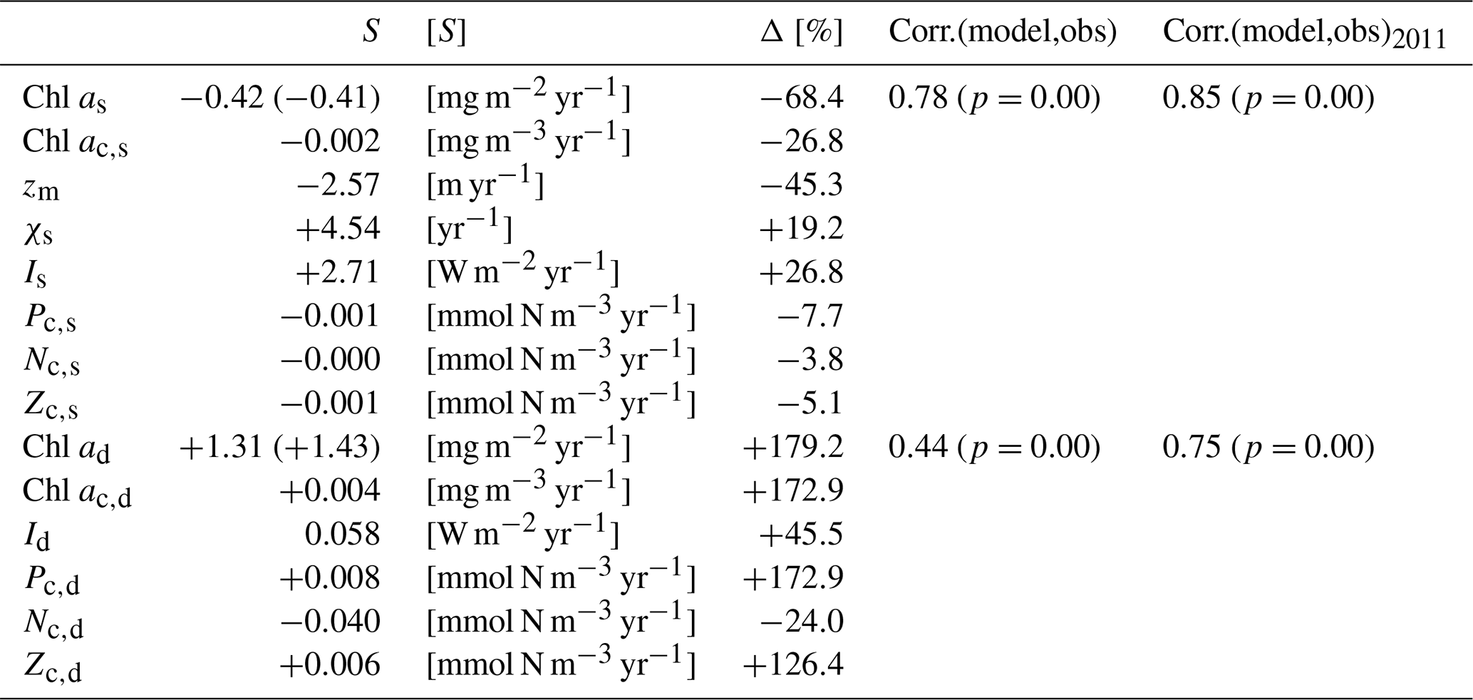
Table 4 The trend and change of state variables from the model over 2011–2022 and the relationship between chlorophyll biomass from the model and observations. In this table, Chl a_s and Chl a_d represent the surface and subsurface integration of the chlorophyll, respectively. Chl a_c,s, z_m, χ_s, I_s, P_c,s, N_c,s, and Z_c,s represent the deseasonalized MLD, surface chlorophyll concentration, surface C:Chl ratio, surface light, surface phytoplankton concentration, surface DIN concentration, and surface zooplankton concentration from the model. Similarly, Chl a_c,d, I_d, P_c,d, N_c,d, and Z_c,d represent the chlorophyll concentration, light, phytoplankton concentration, DIN concentration, and zooplankton concentration at the subsurface layer from the model. S means the slope of the post-2011 trend of the parameters mentioned above. All S values are significant except for the trend of Z_c,s. The unit of S for each parameter is shown as [S] in square brackets. Δ denotes the percentage change in the fitted model output for each parameter described above between 1 January 2011 and 31 December 2022. The values from the observations are shown in parenthesis and the rest of the values are from the model. The correlation coefficient, Corr.(model,obs), shows the relationship between the deseasonalized full time series over 1990–2022 in the model and observations; its corresponding p value is shown in parentheses. Similarly, Corr.(model,obs)₂₀₁₁ shows the relationship between the deseasonalized time series over 2011–2022 in the model and observation.

3.3 Drivers of post-2011 trend in chlorophyll a in the two layers

The deseasonalized chlorophyll stocks (Chl a_s) at the surface layer over 1990–2022 from the model (solid green line) and observations (solid black line) are shown in Fig. 5a. They show very good agreement reflected by a significant positive correlation coefficient (0.78) shown in Table 4. This coefficient even increases to 0.85 if only comparing the deseasonalized Chl a_s over 2011–2022 (Table 4). This suggests that this two-layer NPZ model has a strong ability to simulate the interannual variability in surface chlorophyll stocks, particularly over 2011–2022.

The observational Chl a_s shows a significant decreasing trend from 2011 to the end of 2022 (straight black line in Fig. 5a), also reported by Viljoen et al. (2024). Table 4 confirms this significant decreasing trend by showing a slope of −0.41 mg m⁻² yr⁻¹ in observations. This decreasing trend post-2011 is also captured in the two-layered model (green line in Fig. 5a), with a very similar trend ($S=-\mathrm{0.42}$ mg m⁻² yr⁻¹ in Table 4) as seen in observations.

Figure 5b shows the deseasonalized subsurface chlorophyll stock time series (Chl a_d) from the model (dashed green line) and observations (dashed black line). Although the correlation is weaker than seen in Chl a_s, it is still significant (Corr. = 0.44 in Table 4). This correlation becomes strong over 2011–2022, reflected by an increase in Corr. to 0.75 (Table 4). This indicates that the model is also capable of simulating the interannual variability of chlorophyll in the subsurface layer, particularly post-2011, although it is weaker than at the surface layer. Looking at 2011–2022, in contrast to the decreasing trend in Chl a_s, Chl a_d shows an increasing trend in both the model and observations (Fig. 5b). Table 4 confirms this increasing trend, showing a similar significant positive slope of the Chl a_d post-2011 trend in the model (S=1.31 mg m⁻² yr⁻¹) and observations (S=1.43 mg m⁻² yr⁻¹).

To understand the drivers of the decreasing trend in Chl a_s over 2011–2022, we first show the interannual variability of the observational mixed layer depth (z_m) (Fig. 5c) and surface chlorophyll concentration (Chl a_c,s) from the model (Fig. 6a). Figure 5c demonstrates a decreasing trend in z_m since 2011 ($S=-\mathrm{2.57}$ m yr⁻¹ in Table 4), which indicates a decreasing trend in the surface layer thickness. However, the chlorophyll concentration also shows a decreasing trend ($S=-\mathrm{0.002}$ mg m⁻³ yr⁻¹), which mirrors the decrease in chlorophyll stocks. Δ of Chl a_c,s is −26.8 %, which means that the chlorophyll concentration decreased by approximately 27 % from 2011 to 2022. This further confirms that the decreasing trend of Chl a_s is related to the decrease in Chl a_c,s rather than purely driven by a decreasing surface layer water volume.

Next, to understand the drivers of decreasing Chl a_c,s post-2011, we also show the surface C:Chl ratio (χ_s), light (I_s), phytoplankton (P_c,s) concentration, nutrient (N_c,s) concentration, and zooplankton (Z_c,s) concentration from the model (Fig. 6b–e). χ_s and I_s show an increasing trend since 2011 (Fig. 6b), reflected by a positive slope of 4.54 yr⁻¹ and 2.71 W m⁻² yr⁻¹, respectively (see Table 4). From 2011 to 2022, χ_s and I_s increase by around 19.2 % and 26.8 %. In contrast to the surface light trend, P_c,s shows a weak decreasing trend ($S=-\mathrm{0.001}$ mmol N m⁻³ yr⁻¹) and a decrease of 7.7 %. N_c,s shows a near-zero decreasing trend and Z_c,s does not show a significant trend (p=0.05), which is also reflected by their small change in percentage of −3.8 % and −5.1 %, respectively. Our results suggest that the change in surface chlorophyll concentration is primarily driven by the change in surface light and χ_s rather than the change in phytoplankton concentration. The shoaling of mixed layer depth (Fig. 5c) described above enhances the light in the surface layer, leading to an increasing C:Chl ratio, which further contributes to a decreasing chlorophyll biomass from 2011 to 2022.

To explore the mechanism behind the increasing Chl a_d trend post-2011, we also show the deseasonalized chlorophyll concentration (Chl a_c,d) in Fig. 7a. Similar to Chl a_d, Chl a_c,d shows an increasing trend (S=0.004 mg m⁻³ yr⁻¹) and increased by 172.9 % from 2011 to 2022 (Table 4). Similarly, this increasing trend is also seen in I_d, P_c,d, and Z_c,d, which show S of 0.058 W m⁻² yr⁻¹, 0.008 mmol N m⁻³ yr⁻¹, and 0.006 mmol N m⁻³ yr⁻¹, respectively. A large change in the percentage is also seen in I_d (+45.5 %), P_c,d (+172.9 %), and Z_c,d (+126.4 %). Particularly, the change in percentage in P_c,d is identical to Chl a_c,d, owing to the fact that the model has a fixed χ_d. These findings suggest that the increase in subsurface chlorophyll biomass is driven by the increase in phytoplankton concentration, which is a result of an increase in light in the subsurface layer due to the shoaling of mixed layer depth and reduction in Chl a_s. This mechanism is further confirmed by a decreasing trend ($S=-\mathrm{0.04}$ mmol N m⁻³ yr⁻¹) and a change in percentage of −24 % in N_c,d, as more nutrients are taken up with subsurface phytoplankton growth.

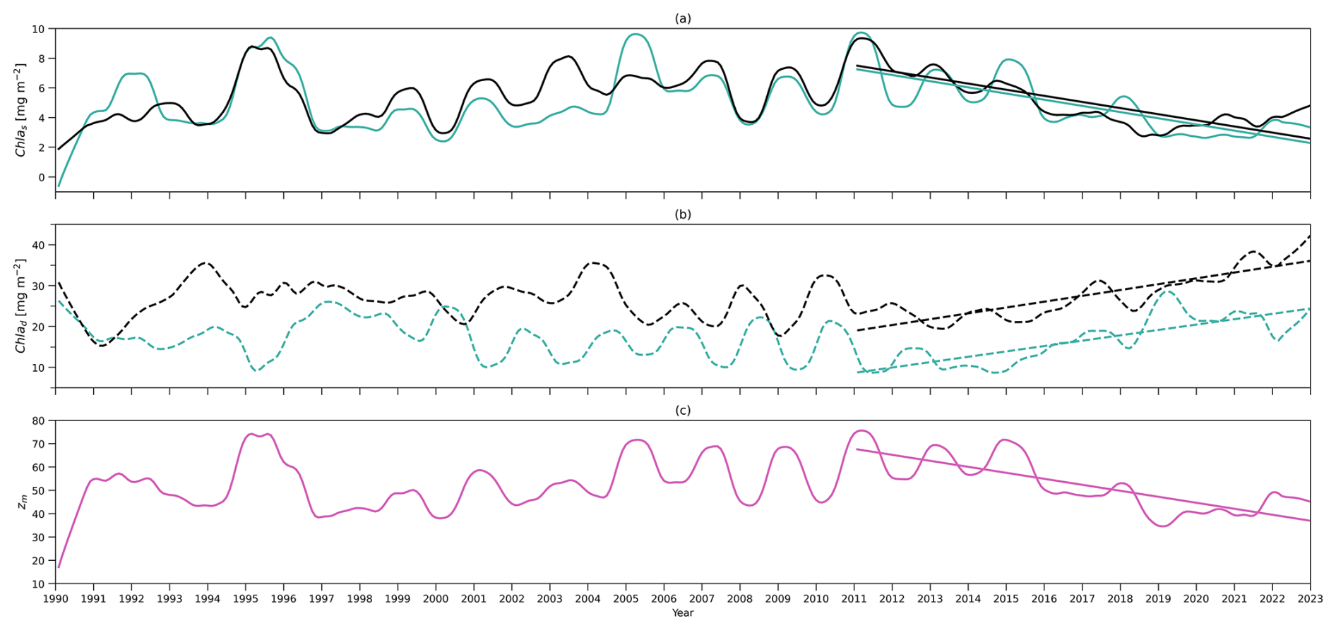
Figure 5 (a) Time series of deseasonalized chlorophyll integration above z_m (surface layer) from 1990 to 2022 from the two-layered NPZ model (green) and from observations (black). Straight lines correspond to the linear regressions fitted to deseasonalized data from 2011 to the end of 2022 (post-2011 includes 2011–2022) from model data (green) and observations (black). (b) As in (a) but for time series of deseasonalized chlorophyll a integration between z_m and z_eu (subsurface layer). (c) As in (a) but for deseasonalized observational MLD (z_m) at BATS.

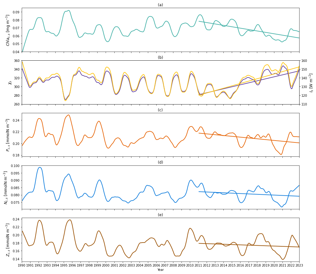
Figure 6 (a) Time series of deseasonalized chlorophyll a concentration vertically averaged above z_m (surface layer) from 1990 to 2022 from the two-layered NPZ model. Straight lines correspond to the linear regressions fitted to deseasonalized data from 2011 to the end of 2022 (post-2011 includes 2011–2022) from model data. (b) Deseasonalized surface C:Chl ratio (purple) and light (yellow) time series from 1990 to the end of 2022 from the two-layered NPZ model. The purple (yellow) straight line indicates the linear regressions fitted to the deseasonalized surface C:Chl ratio (light) data from 2011 to the end of 2022 (post-2011 includes 2011–2022) from the two-layered NPZ model. (c) As in (a) but for the deseasonalized surface phytoplankton concentration from the model. (d) As in (e) but for the deseasonalized surface DIN concentration from the model. (e) As in (a) but for the deseasonalized surface zooplankton concentration from the model.

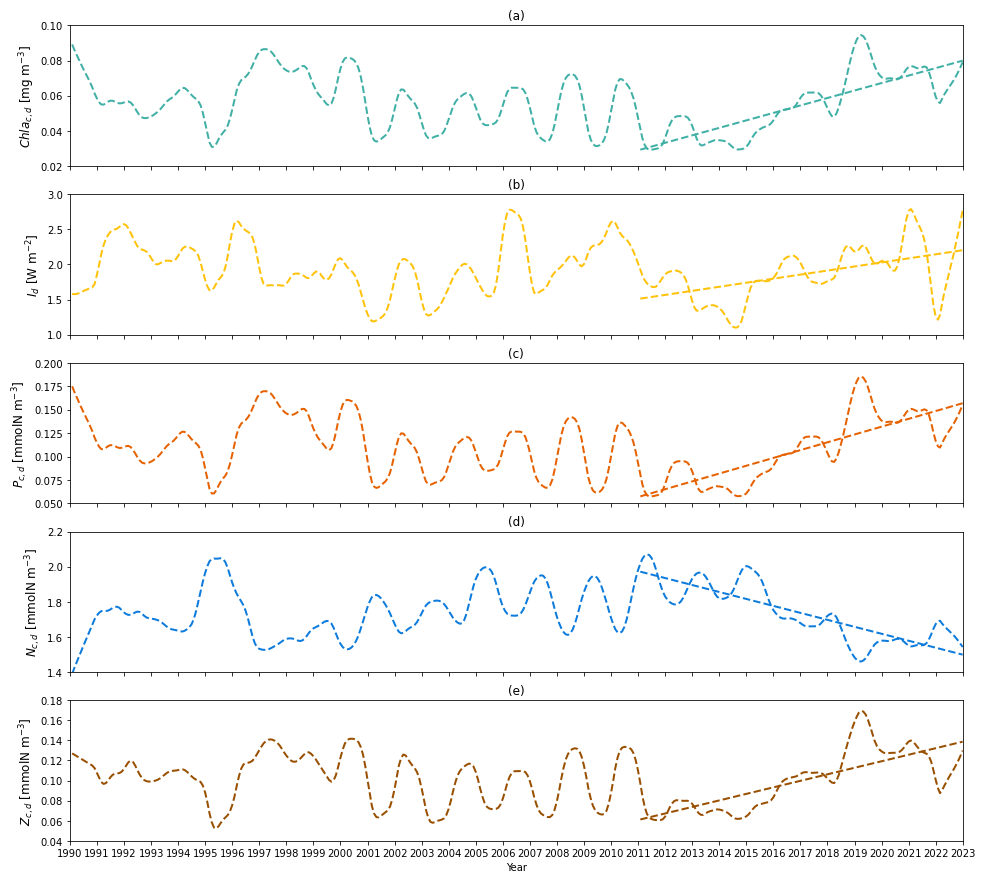
Figure 7 (a) Time series of deseasonalized chlorophyll a concentration vertically averaged between z_m and z_eu (subsurface layer) from 1990 to 2022 from the two-layered NPZ model. Straight lines correspond to the linear regressions fitted to deseasonalized data from 2011 to the end of 2022 (post-2011 includes 2011–2022) from model data. (b) As in (a) but for deseasonalized subsurface light time series from 1990 to the end of 2022 from the two-layered NPZ model. (c) As in (a) but for the deseasonalized subsurface phytoplankton concentration from the model. (d) As in (e) but for the deseasonalized subsurface DIN concentration from the model. (e) As in (a) but for the deseasonalized subsurface zooplankton concentration from the model.

4 Discussion

We have built a two-layered NPZ box model of the stratified ocean that assumes the marine ecosystem in the euphotic zone can be partitioned into two distinct communities: one located within the mixed layer and the other situated below the mixed layer and above the very base of the euphotic zone (defined here as the 0.0001 % light level). These two communities reside in two different environments: a (typically) nutrient-limited one within the mixed layer and a light-limited one below it.

Model estimates of the time-mean vertically averaged phytoplankton concentration are 0.21 mmol N m⁻³ in the surface layer (above the mixed layer depth) and 0.12 mmol N m⁻³ in the subsurface layer (below the mixed layer and above the euphotic zone). These estimates align well with the near-surface value given by Kantha (2004) (0.2 mmol N m⁻³) and the time-mean range of 0.05–0.15 mmol N m⁻³ at a depth of 100–250 m simulated by the coupled physical and NPZD model of Doney et al. (1996). Similarly, this model estimates a time-mean surface chlorophyll concentration of 0.07 mg m⁻³, which is consistent with the estimate (around 0.09 mg m⁻³) modelled by an NPZD model at BATS (Spitz et al., 2001) and the time mean from observations (around 0.1 mg m⁻³) (Anugerahanti et al., 2020). Also, this model provides a range of 0–0.33 mg m⁻³ for the chlorophyll concentration at the subsurface layer, which is consistent with the observational range of 0–0.25 mg m⁻³ and modelling range of 0–0.35 mg m⁻³ given by Anugerahanti et al. (2020).

Regarding zooplankton, limited by fixed observations at 200 m at BATS (Madin et al., 2001), we cannot make a direct comparison of our model estimates with these observations. Nonetheless, our model provides comparable time-mean zooplankton concentration estimates of 0.18 mmol N m⁻³ above the mixed layer and 0.1 mmol N m⁻³ below it, which are consistent with those reported by Anugerahanti et al. (2020). They utilize a complex 3D ecosystem model (MEDUSA) to reveal a vertical profile of zooplankton concentration ranging from 0 to 0.3 mmol N m⁻³ near the surface decreasing to 0–0.1 mmol N m⁻³ at 200 m (Anugerahanti et al., 2020).

Vertically averaged concentrations of modelled dissolved inorganic nitrogen (DIN) in the two layers align with other studies at BATS. The time mean of DIN concentration averaged within the mixed layer is around 0.09 mmol N m⁻³ in very good agreement with in situ data for DIN at BATS of around 0.1 mmol N m⁻³ within the upper 50 m (Anugerahanti et al., 2020; Hurtt and Armstrong, 1999). The DIN concentration within the mixed layer shows a range of 0.04–0.5 mmol N m⁻³, which is also consistent with the range (0–0.6 mmol N m⁻³) modelled by Spitz et al. (2001). In addition to the surface layer, the subsurface time-mean DIN concentration vertically averaged below the mixed layer and above the euphotic zone (1.73 mmol N m⁻³) in our model agrees with the observational nitrate concentration record (1.75 mmol N m⁻³; Anugerahanti et al., 2018) and modelling output at 160 m (of around 2 mmol N m⁻³) from a 1D algal-group-based phytoplankton model (Salihoglu et al., 2008).

Our model simulates the vertically integrated chlorophyll for two ecosystems using a dynamical model of the C:Chl ratio at the surface layer and a fixed C:Chl ratio at the subsurface layer. The chlorophyll integration within the mixed layer in this model shows a strong seasonal cycle with a maximum (13.63 mg m⁻²) in spring and a minimum (0.52 mg m⁻²) in summer, in good agreement with in situ observations at BATS. Furthermore, this seasonality closely matches the median climatology (around 2.5–18.5 mg m⁻²) of the surface chlorophyll integration partitioned from the vertical profiles using a sigmoid-based function (Viljoen et al., 2024). Although different integration boundaries make more direct comparisons with other studies difficult, the range of chlorophyll integrations is also comparable with modelling and observations reported by Doney et al. (1996) within the upper 140 m (10–30 mg m⁻²) at BATS.

Both model and in situ data show that phytoplankton in the two layers have a contrasting seasonality at BATS, which is also seen in the statistical partition results of Viljoen et al. (2024) and in other seasonally stratified regions like the northern Red Sea (Brewin et al., 2022). The subsurface chlorophyll stock shows a seasonality with a minimum (1.89 mg m⁻²) in spring and a maximum (39.94 mg m⁻²) in autumn. The maximum matches the in situ measurements (35.24 mg m⁻²), while the minimum displays a larger discrepancy from observations (11.57 mg m⁻²) in spring. However, this minimum value estimated from our two-layered model agrees with the minimum (near zero) of the chlorophyll integration below the mixed layer partitioned using a conceptual model applied to vertical profiles in Viljoen et al. (2024). The former maximum from our models is also comparable to but higher than the maximum of their median chlorophyll integration climatology (around 20 mg m⁻²) (Viljoen et al., 2024). This discrepancy may be attributed to the deeper integration boundary used in our model and also the different choice of climatology (time mean and median) (Viljoen et al., 2024). Given that measurements below 50 m are scarcer, especially in spring (Anugerahanti et al., 2020), than near-surface measurements, the values predicted by our model may still be considered reasonable.

Concerns may be raised regarding the choice of different bottom boundaries when comparing modelled subsurface-integrated chlorophyll against the observations. A sensitivity analysis based on different euphotic zone assumptions (see Appendix A) shows that different assumptions primarily influence the seasonality comparison, particularly in summer when the subsurface layer (water column) in the model is thicker compared to winter. A shallower euphotic zone could cause the model to overestimate integrated chlorophyll in summer, whereas a deeper euphotic zone might make observations not suitable for model validation due to lack of measurements. Despite these potential uncertainties related to the euphotic zone, the interannual variability comparison is hardly influenced by different definitions of euphotic zones.

This model simulates a strong seasonality in DIN stocks accumulated within the mixed layer, in agreement with in situ data (Fig. 4c and g). It shows a peak (11.04 mmol N m⁻²) in spring, agreeing with the peak value from in situ measurements (10.25 mmol N m⁻²) of NO₂ + NO₃ stocks, and a minimum (1.21 mmol N m⁻²) in summer, slightly higher than shown in observations (0.04 mmol N m⁻²). These lower values (near zero) of in situ measurements during summer and autumn are limited by the sensitivity of the method used for measuring DIN (Steinberg et al., 2001; Lomas et al., 2013), which is unable to resolve low concentrations of DIN. Thus, our estimate could be a reasonable representative of the seasonal minimum surface DIN stocks.

Our results underscore the challenge of accurately simulating subsurface communities, likely due to difficulties in accurately determining parameters for the subsurface layer. Modelling subsurface nitrate dynamics, especially seasonality, is particularly challenging with a simplified model. Despite this, our model aligns with observed time-mean DIN values (around 460 mmol N m⁻²), closely matching NO₂ + NO₃ integrated stocks (468 mmol N m⁻²). Moreover, while uncertainties in deep-ocean nitrate dynamics remain, these have a minimal effect on subsurface phytoplankton growth, which is driven by subsurface light. Sensitivity analysis further emphasizes the importance of determining subsurface parameters for simulating subsurface chlorophyll and nutrient dynamics. Although the parameters for the subsurface layer in our model are derived from the assimilation of the observational data at BATS (e.g. Schartau and Oschlies, 2003), there is a need for more precise parameterizations tailored to the specific subsurface environment to enhance our understanding of phytoplankton communities' responses to climate change. This can only be achieved by modellers working together with observers, targeting key measurements of important subsurface parameters, and improving understanding of controls on subsurface phytoplankton.

Some studies have observed increasing trends in integrated chlorophyll at BATS (e.g. 150 m integration from 1989 to 2003; Saba et al., 2010). However, recently, Viljoen et al. (2024) observed the opposite trends in surface and subsurface chlorophyll integration between 2011 and 2022. This opposite trend is also captured in this two-layered model. Our model reveals that shoaling mixed layer depth increases the light availability at both the surface and subsurface layers. However, the two phytoplankton communities at the surface and subsurface layers show different responses to this increase in light intensity. At the surface layer, the C:Chl ratio in this model shows an increasing trend over 2011–2022, which is also seen from Viljoen et al. (2024). This change in C:Chl ratio explains most of the change in surface chlorophyll biomass. Although our model shows a decreasing trend in phytoplankton concentration, whereas Viljoen et al. (2024) showed no trend in surface, this change is small (7.7 %), and there is little trend in surface nutrient concentration and no trend in zooplankton. This supports the mechanism at the surface layer observed in Viljoen et al. (2024) that intensifying light does not directly drive a decrease in carbon stocks; instead, it changes the physiology of phytoplankton by increasing the C:Chl ratio, which leads to a decreasing chlorophyll biomass over 2011–2022. Different from the surface layer, an increasing trend in chlorophyll stocks is still seen from both observations and our model. This is because the growth of phytoplankton is purely driven by the light in the subsurface and the C:Chl ratio is fixed. The intensifying light directly leads to an increase in phytoplankton and chlorophyll biomass, confirmed by the large consistent change in subsurface light as well as the chlorophyll, phytoplankton, and zooplankton concentration, which also agrees with the observations in Viljoen et al. (2024). Understanding these mechanisms will help improve projections of future chlorophyll stocks in stratified systems with ocean warming.

Despite our model providing valuable insights into vertical variations in plankton community composition and helping to understand drivers of trends during the past decade at BATS, it is important to acknowledge its limitations. The processes designed in this model do not incorporate all the key biogeochemical processes in stratified systems, such as nitrogen fixation and iron limitation, which should be considered in future developments. Moreover, the model does not explicitly account for important biological components such as bacteria, viruses, and detritus, which play a crucial role in nutrient cycling and ecosystem functioning. Our model does not incorporate the diversity of phytoplankton or zooplankton within the two layers. It also assumes the conservation of phytoplankton and nutrients within the mixed layer during shoaling, which may overestimate the surface phytoplankton, as they could be lost from the surface layer when the mixed layer shoals. We also assume that the two vertically separated communities of phytoplankton and zooplankton do not directly interact, only implicitly through the exchange in nutrients between layers. Good agreement between model output and observations supports this assumption. Our model assumes a linear relationship between nutrients interacting between the two layers and the depth of the mixed layer. In cases where this relationship is not linear, our model may not be appropriate to use. We have explored including an explicit entrainment term in our model to capture some nonlinearity (see Appendix B). This term exchanges phytoplankton between layers through entrainment (term not included for zooplankton, assuming they are motile). The entrained phytoplankton are converted directly to nutrients assuming competitive exclusion (see Appendix B). Including this process had little influence on our results at the BATS location. However, this process may play a more important role in other regions. Future work should investigate if an explicit interaction between zooplankton would further improve model simulations. There are also other limitations related to model application. As a two-layered box model, coupling it with other more complex physical models may not be straightforward. Furthermore, the parameters presented in this study are specifically designed for the BATS site and will likely require adjustment for other stratified locations.

5 Summary

We developed a two-layer NPZ model for stratified oceans, partitioning the euphotic zone into a surface layer above the mixed layer depth and a subsurface layer below it for the first time. The model applies distinct parameters in each layer to capture the contrasting environmental conditions for phytoplankton growth at BATS.

This simple model was able to simulate the chlorophyll seasonal and interannual variability at both the surface and subsurface layers, reproducing the observed contrasting trends in chlorophyll between the two layers over the past decade.

The model simulations, along with the accompanying sensitivity analyses, reveal that the main mechanisms responsible for the decreasing trend in surface chlorophyll in recent years at the Bermuda time series site are two-fold: (a) increasing trend in light reaching the surface layer at the study site and associated photo-acclimation, as indicated by changes in the carbon to chlorophyll ratio in phytoplankton, and (b) changes in stratification and an associated decrease in the mixed layer depth. Interestingly, the model also captures with high fidelity the contrasting seasonal patterns in chlorophyll dynamics in the subsurface layer, as well as the contrasting increasing trend in the subsurface chlorophyll in recent years. Key to the success of the simulation has been the treatment of the phytoplankton communities in the two layers as distinct communities with distinct bio-optical and physiological traits adapted to the local environment.

The study underscores the importance of following changes in both the layers to be able to appreciate and predict any current or future changes in marine ecosystems as a whole in response to changing climate. We see here that the decrease in surface chlorophyll as a result of increasing stratification may be compensated for by a corresponding increase in subsurface chlorophyll. Though the detrimental effect of increasing stratification on surface chlorophyll is often discussed in the literature, the beneficial effects on the subsurface phytoplankton communities are often overlooked.

Generalizing the model to other regions can only be undertaken cautiously because many of the simplifications applied to the model were designed to mimic the local conditions at the study site; this includes, for example, a high level of decoupling between the two layers due to stratification, which may not be applicable elsewhere. The strength of the model lies in being able to follow the contrasting dynamics of the surface and subsurface populations of phytoplankton as distinct communities that are simulated using model parameters appropriate for each community.

Appendix A: Sensitivity analysis of euphotic zone depth

To explore the impact of different euphotic zone depth definitions on subsurface chlorophyll integration and its comparison with observations, we conducted a sensitivity analysis using alternative euphotic zone criteria.

In the main paper, the euphotic zone is defined as the depth corresponding to 0.0001 % of the surface light level. Accordingly, in this sensitivity analysis, we defined the euphotic zone as 0.001 % (shallower euphotic zone) and 0.00001 % (deeper euphotic zone) of the surface light level. By running the model with these two extra euphotic zone assumptions, the subsurface chlorophyll integrations are simulated. Accordingly, the observations are recalculated using these new bottom boundaries following the method described in Sect. 2.4.

Figures A2 and A3 demonstrate the subsurface chlorophyll integration based on 0.001 % and 0.00001 % light-level-based euphotic zones, respectively (green lines). Accordingly, they also show the new observational subsurface chlorophyll integration (black dots) calculated from 0.001 % and 0.00001 % euphotic zones separately. Compared with Fig. 4f, the main effect of different definitions of the euphotic zone on subsurface chlorophyll integration comparison occurs in summer (June–August). Given that the mixed layer depth is typically shallow in summer, this results in a thicker subsurface layer. In this case, changes in the bottom boundary have a stronger impact on subsurface light and accordingly the chlorophyll concentration.

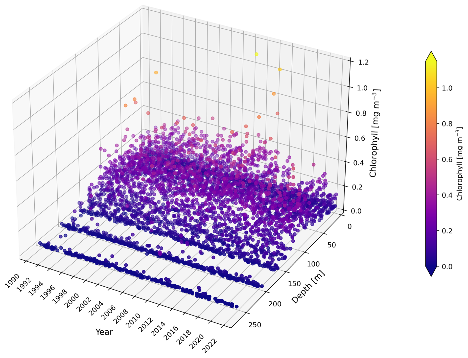
Figure A1 Vertical distribution of chlorophyll concentration [mg m⁻³] measurements at BATS from 1990 to 2022. Observational data are plotted as a function of depth (from the sea surface at 0 m to the deep layers) and year, with colour representing the chlorophyll concentration.

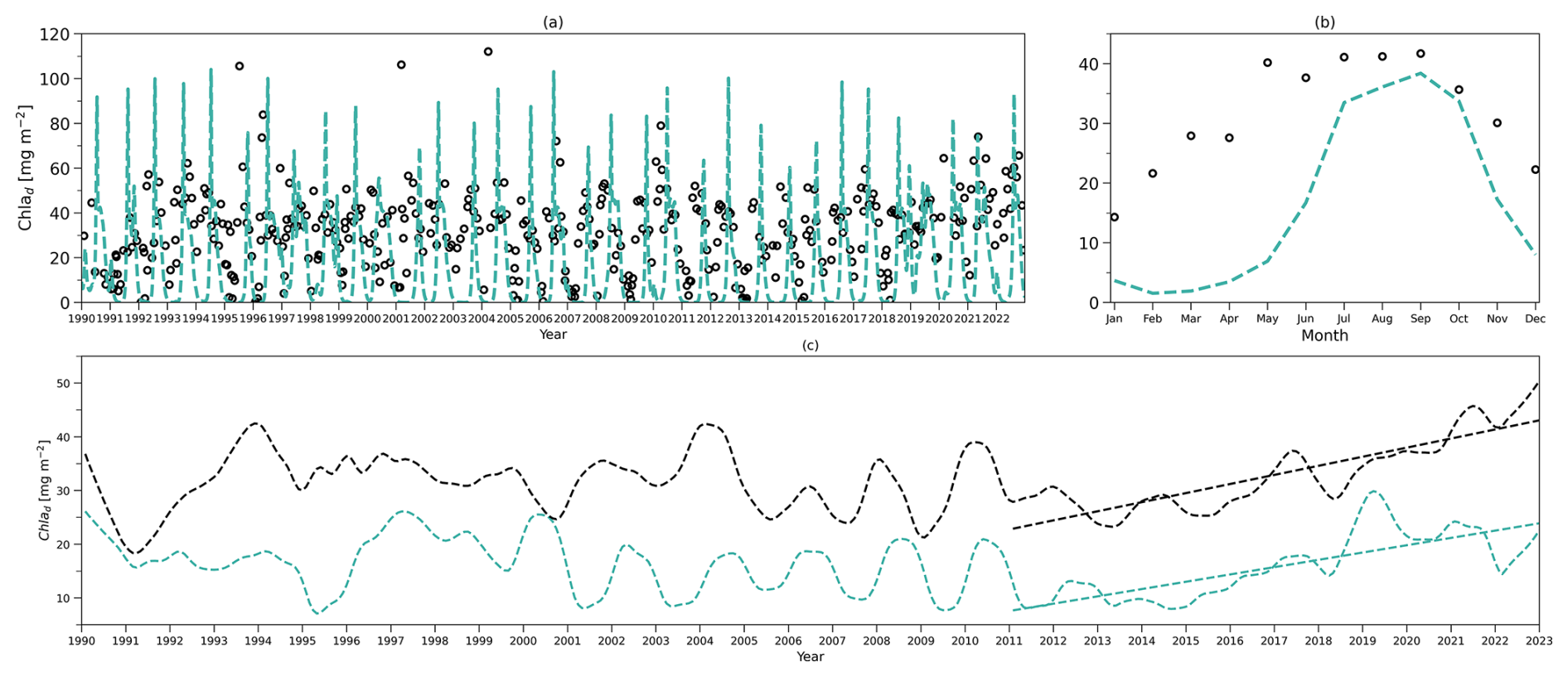
Specifically, a shallower euphotic zone tends to cause the model to increase subsurface chlorophyll integration in summer (Fig. A2b), whereas a deeper euphotic zone leads to a reduction (Fig. A3b). The water column used for integration calculations remains consistent across comparisons, so differences between model simulations and observations arise mainly from variations in modelled and observational representative chlorophyll concentrations under different euphotic zone depths. A shallower euphotic zone generally leads the model to increase chlorophyll concentrations in summer. In contrast, a deeper euphotic zone reduces the subsurface chlorophyll concentration in summer. However, we need to be careful about the observational representative concentration. Given that there are no chlorophyll measurements below the 0.0001 % euphotic zone (see Fig. A1), a deeper (0.00001 %) euphotic zone can inflate the observational chlorophyll concentration.

Despite these impacts on seasonality comparisons, different euphotic zones have a minimal impact on the post-2011 trend comparison in subsurface chlorophyll integration. Figures A2c and A3c show that the modelled trend remains similar to observations, consistent with the results presented in Fig. 5b. In conclusion, varying the euphotic zone assumptions primarily affects seasonal comparisons between the model and observations but does not change our primary findings regarding post-2011 trends.

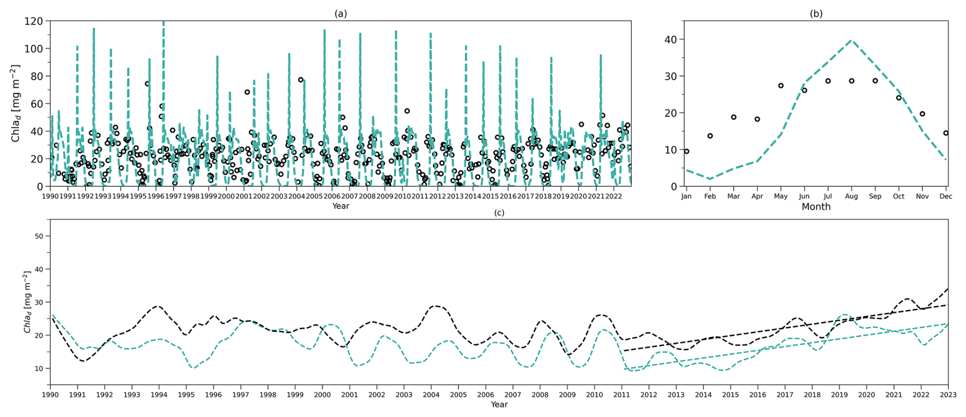
Figure A2 Comparison of chlorophyll integration between the model and observations using a euphotic zone defined by the 0.001 % surface light level. (a) Daily chlorophyll stocks at the subsurface layer from the model (dashed green line) and observations (hollow dark dots) from 1990 to 2022. (b) As in (a) but for the time-mean climatology. (c) Deseasonalized subsurface chlorophyll integration time series from 1990 to 2022 from the two-layered NPZ model (green) and from observations (black). Straight lines correspond to the linear regressions fitted to deseasonalized data from 2011 to the end of 2022 (post-2011 includes 2011–2022) from model data (green) and observations (black).

Figure A3 As in Fig. A2, but based on the euphotic zone defined as 0.00001 % of the surface light level.

Appendix B: MLD-driven phytoplankton interactions

To explore the influence of the mixed layer depth pump on two phytoplankton communities across two layers, we include additional interactions of two phytoplankton communities during mixing processes by modifying the equations presented in Sect. 2.1. We implicitly assumed that each phytoplankton community dominates competition in each layer. When these communities interact driven by oscillations of MLD, the superior competitor immediately outcompetes the other. Specifically, when the mixed layer depth deepens, phytoplankton in the subsurface layer that are carried to the surface layer (simulated by ${\mathit{\zeta }}^{+}\left(t\right)P_{\mathrm{c},\mathrm{d}}$ in Eq. B6) directly die off and directly convert to the surface nutrient pool (Eq. B2) as this model excludes the detrital state variable. We also introduced ζ⁻(t) (see Eq. B1) to help simulate the opposite scenario of a shallowing mixed layer during which phytoplankton from the surface layer (${\mathit{\zeta }}^{-}\left(t\right)P_{\mathrm{c},\mathrm{d}}$) are advected to the subsurface layer, contributing to the subsurface nutrient pool (see Eq. B4).

To maintain consistency with phytoplankton processes, we similarly apply this mixed layer pump concept for nutrients, replacing the traditional asymmetrical MLD effect (by deleting ${\mathit{\zeta }}^{+}\left(t\right)(N_{\mathrm{c},\mathrm{d}}-N_{\mathrm{c},\mathrm{s}})$). When the mixed layer depth deepens (denoted by ζ⁺(t) in Eq. 1), nutrients from the subsurface layer (N_c,d) are transported to the surface layer, explicitly represented by ${\mathit{\zeta }}^{+}\left(t\right)N_{\mathrm{c},\mathrm{d}}$ in Eqs. (B2) and (B4). In contrast, when the mixed layer depth shallows (ζ⁻(t) in Eq. B1), nutrients from the surface layer are advected to the subsurface layer shown as ${\mathit{\zeta }}^{-}\left(t\right)N_{\mathrm{c},\mathrm{s}}$ in Eqs. (B2) and (B4).

In summary, we introduced a new equation (Eq. B1) and adjusted the surface nutrient (Eq. 5) and phytoplankton (Eq. 6) concentration equations to become Eqs. (B2) and (B3), respectively. Similarly, the subsurface nutrient (Eq. 17) and phytoplankton (Eq. 18) concentration equations become Eqs. (B4) and (B5), respectively. All other equations from Sect. 2.1 remain unchanged.

$$\begin{array}{}\text{(B1)}& {\displaystyle }{\mathit{\zeta }}^{-}\left(t\right)=min(\mathrm{0},\mathit{\zeta }(t\left)\right),\text{(B2)}& {\displaystyle }\begin{array}{rl}{\displaystyle \frac{\mathrm{d}{N}_{\mathrm{c},\mathrm{s}}}{\mathrm{d}t}}& =-G_{\mathrm{s}}{P}_{\mathrm{c},\mathrm{s}}+{\mathit{\mu }}_p{m}_{\mathrm{s}}{P}_{\mathrm{c},\mathrm{s}}+(\mathrm{1}-{\mathit{\gamma }}_{\mathrm{s}}-{\mathit{\mu }}_g){\mathrm{\Phi }}_{\mathrm{s}}{Z}_{\mathrm{c},\mathrm{s}}\\ & +{\mathit{\mu }}_z{c}_{\mathrm{s}}{Z}_{\mathrm{c},\mathrm{s}}^{\mathrm{2}}-{\displaystyle \frac{\mathit{\zeta }\left(t\right)}{z_{\mathrm{m}}}}{N}_{\mathrm{c},\mathrm{s}}+{\displaystyle \frac{\left({\mathit{\mu }}_{\mathrm{m}}{z}_{\mathrm{m}}\right)(N_{\mathrm{c},\mathrm{d}}-N_{\mathrm{c},\mathrm{s}})}{z_{\mathrm{m}}}}\\ & +{\displaystyle \frac{{\mathit{\zeta }}^{+}\left(t\right)P_{\mathrm{c},\mathrm{d}}}{z_{\mathrm{m}}}}+{\displaystyle \frac{{\mathit{\zeta }}^{+}\left(t\right)N_{\mathrm{c},\mathrm{d}}}{z_{\mathrm{m}}}}+{\displaystyle \frac{{\mathit{\zeta }}^{-}\left(t\right)N_{\mathrm{c},\mathrm{s}}}{z_{\mathrm{m}}}},\end{array}\text{(B3)}& {\displaystyle }\begin{array}{rl}{\displaystyle \frac{\mathrm{d}{P}_{\mathrm{c},\mathrm{s}}}{\mathrm{d}t}}& =G_{\mathrm{s}}{P}_{\mathrm{c},\mathrm{s}}-m_{\mathrm{s}}{P}_{\mathrm{c},\mathrm{s}}-{\mathrm{\Phi }}_{\mathrm{s}}{Z}_{\mathrm{c},\mathrm{s}}-{\displaystyle \frac{\mathit{\zeta }\left(t\right)}{z_{\mathrm{m}}}}{P}_{\mathrm{c},\mathrm{s}}\\ & +{\displaystyle \frac{{\mathit{\zeta }}^{-}\left(t\right)P_{\mathrm{c},\mathrm{s}}}{z_{\mathrm{m}}}},\end{array}\text{(B4)}& {\displaystyle }\begin{array}{rl}{\displaystyle \frac{\mathrm{d}{N}_{\mathrm{c},\mathrm{d}}}{\mathrm{d}t}}& =-G_{\mathrm{d}}{P}_{\mathrm{c},\mathrm{d}}+m_{\mathrm{d}}{P}_{\mathrm{c},\mathrm{d}}+(\mathrm{1}-{\mathit{\gamma }}_{\mathrm{d}}){\mathrm{\Phi }}_{\mathrm{d}}{Z}_{\mathrm{c},\mathrm{d}}\\ & +c_{\mathrm{d}}{Z}_{\mathrm{c},\mathrm{d}}^{\mathrm{2}}-{\displaystyle \frac{\mathit{\eta }\left(t\right)}{z_D}}{N}_{\mathrm{c},\mathrm{d}}+\mathit{\varphi }\\ & -{\displaystyle \frac{\left({\mathit{\mu }}_{\mathrm{m}}{z}_{\mathrm{m}}\right)(N_{\mathrm{c},\mathrm{d}}-N_{\mathrm{c},\mathrm{s}})}{z_D}}-{\displaystyle \frac{{\mathit{\zeta }}^{-}\left(t\right)P_{\mathrm{c},\mathrm{s}}}{z_D}}\\ & -{\displaystyle \frac{{\mathit{\zeta }}^{+}\left(t\right)N_{\mathrm{c},\mathrm{d}}}{z_D}}-{\displaystyle \frac{{\mathit{\zeta }}^{-}\left(t\right)N_{\mathrm{c},\mathrm{s}}}{z_D}},\end{array}\text{(B5)}& {\displaystyle }\begin{array}{rl}{\displaystyle \frac{\mathrm{d}{P}_{\mathrm{c},\mathrm{d}}}{\mathrm{d}t}}& =G_{\mathrm{d}}{P}_{\mathrm{c},\mathrm{d}}-m_{\mathrm{d}}{P}_{\mathrm{c},\mathrm{d}}-{\mathrm{\Phi }}_{\mathrm{d}}{Z}_{\mathrm{c},\mathrm{d}}\\ & -{\displaystyle \frac{\mathit{\eta }\left(t\right)}{z_D}}{P}_{\mathrm{c},\mathrm{d}}-{\displaystyle \frac{{\mathit{\zeta }}^{+}\left(t\right)P_{\mathrm{c},\mathrm{d}}}{z_D}}.\end{array}\end{array}$$

Next, running the model with these modified equations, we show the chlorophyll and nutrient integration from the model and observations (Fig. B1). The results obtained from these simulations were very similar to those presented in Fig. 4. We also present the deseasonalized chlorophyll integration from the model and observations in Fig. B2, which also closely match the patterns in Fig. 5. Consequently, our main conclusions remain robust, even when incorporating this more complex mixing scenario driven by mixed layer depth variations.

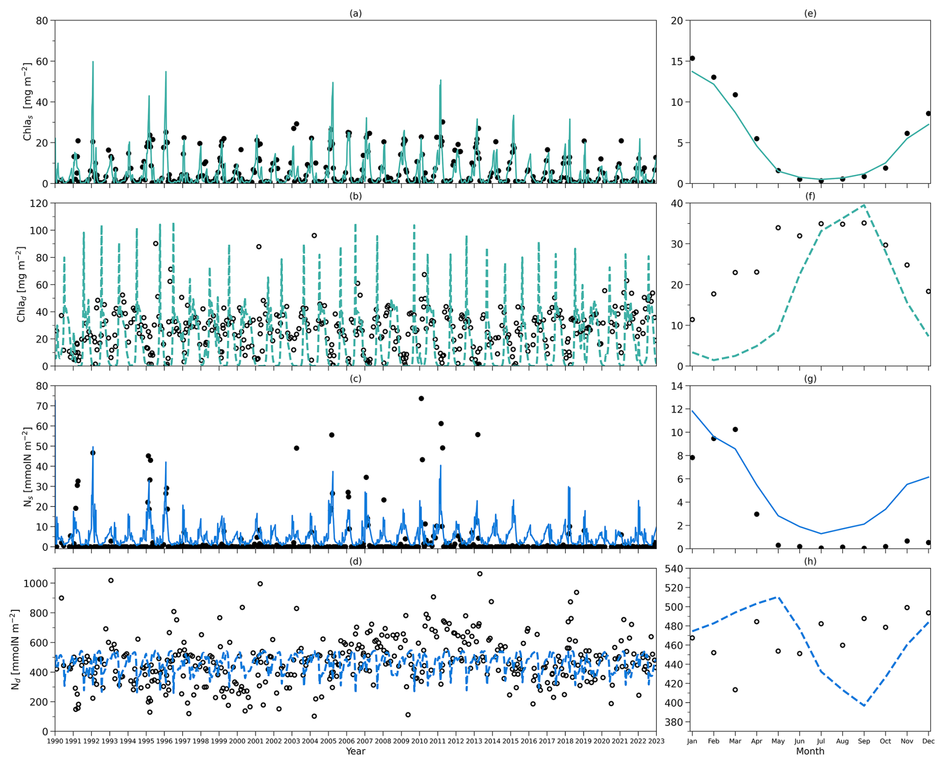
Figure B1 (a) Daily chlorophyll stocks at the surface layer from the model (solid green line) and observations (solid dark dots) from 1990 to 2022. (b) Daily chlorophyll stocks at the subsurface layer from the model (dashed green line) and observations (hollow dark dots) from 1990 to 2022. (c) Daily nitrogen stocks at the surface layer from the model (solid blue line) and observations (hollow dark dots) from 1990 to 2022. (d) Daily nitrogen stocks at the subsurface layer from the model (dashed blue line) and observations (hollow dark dots) from 1990 to 2022. Panels (e)–(h) are as in (a)–(d) but for their time-mean climatology. Results are from simulations using Eqs. (B1)–(B5).

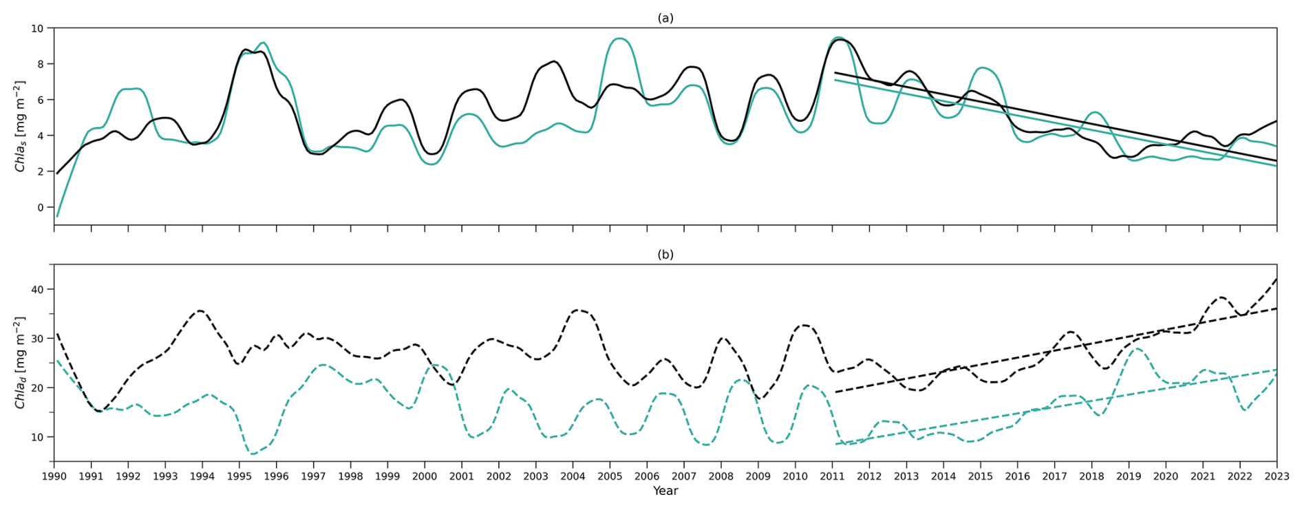
Figure B2 (a) Deseasonalized chlorophyll integration above z_m (surface layer) time series from 1990 to 2022 from the two-layered NPZ model (green) and from observations (black). Straight lines correspond to the linear regressions fitted to deseasonalized data from 2011 to the end of 2022 (post-2011 includes 2011–2022) from model data (green) and observations (black). (b) As in (a) but for deseasonalized chlorophyll a integration between z_m and z_eu (subsurface layer) time series. Results are from simulations using Eqs. (B1)–(B5).